integrating cognitive process and descriptive models of - newcl.org
TRANSCRIPT
Integrating Cognitive Process and Descriptive Models ofAttitudes and Preferences
Guy E. Hawkinsa, A.A.J. Marleyb,c, Andrew Heathcoted, Terry N.Flynnc, Jordan J. Louvierec, and Scott D. Brownda School of Psychology, University of New South Wales, Australia
b Department of Psychology, University of Victoria, Canadac Centre for the Study of Choice, University of Technology, Sydney, Australia
d School of Psychology, University of Newcastle, Australia
Abstract
Discrete choice experiments – selecting the best and/or worst from a set ofoptions – are increasingly used to provide more efficient and valid measure-ment of attitudes or preferences than conventional methods such as Likertscales. Discrete choice data have traditionally been analyzed with randomutility models that have good measurement properties, but provide lim-ited insight into cognitive processes. We extend a well-established cognitivemodel, which has successfully explained both choices and response timesfor simple decision tasks, to complex multi-attribute discrete choice data.The fits, and parameters, of the extended model for two sets of choice data(involving patient preferences for dermatology appointments, and consumerattitudes towards mobile phones) agree with those of standard choice mod-els. The extended model also accounts for choice and response time data ina perceptual judgment task designed in a manner analogous to best-worstdiscrete choice experiments. We conclude that a variety of fields can ben-efit from discrete choice experiments, especially when extended to includeresponse time and combined with analyses based on evidence accumulationmodels.
Keywords: Preference; Decision-Making; Best-Worst Scaling; Linear Bal-listic Accumulator; Evidence Accumulation; Random Utility Models.
Correspondence concerning this article may be addressed to: Guy Hawkins, School of Psychology, Uni-versity of New South Wales, Sydney NSW 2052, Australia; Email: [email protected].

BEST-WORST LBA 2
Introduction
Many fields rely on the elicitation of preferences. However, direct questioning meth-ods, such as Likert scales, suffer from well-established drawbacks due to subjectivity (fora summary see Paulhus, 1991). Discrete choice – for example, choosing a single preferredproduct from a range of presented options – provides more reliable and valid measure-ment of preference in areas including health care (Ryan & Farrar, 2000; Szeinbach, Barnes,McGhan, Murawski, & Corey, 1999), personality measurement (Lee, Soutar, & Louviere,2008), and marketing (Mueller, Lockshin, & Louviere, 2010). More efficient and richerdiscrete-choice elicitation is provided by best-worst scaling, where respondents select boththe best option and worst option from a set of alternatives. For example, a respondentpresented with six bottles of wine might be asked to report their most and least preferredbottles. Data collection using best-worst scaling has been increasingly used, particularly instudying consumer preference for goods or services (Collins & Rose, 2011; Flynn, Louviere,Peters, & Coast, 2007, 2008; Lee et al., 2008; Louviere & Flynn, 2010; Louviere & Islam,2008; Marley & Pihlens, 2012; Szeinbach et al., 1999).
In applied fields, best-worst data are often analyzed using conditional logit (alsocalled multinomial logit, MNL) models; the basic model is also known in cognitive scienceas the Luce choice model (Luce, 1959). These models assume that each option has a utility(u, also called “valence” or “preference strength”) and that choice probabilities are simple(logit) functions of those utilities (Finn & Louviere, 1992; Marley & Pihlens, 2012).1 MNLmodels provide compact descriptions of data and can be interpreted in terms of (random)utility maximization, but afford limited insight into the cognitive processes underpinningthe choices made. Further, they do not address choice response time,2 a measure that isincreasingly easy to obtain as data collection becomes computerized.
We explore the application of evidence accumulation models – more often employedto explain simple perceptual choice tasks – to the complex decisions involved in best-worstchoice between multi-attribute options. Our application bridges a divide between relativelyindependent advances in theoretical cognitive science (computational models of cognitionsunderlying simple decisions) and applied psychology (best-worst scaling to elicit maximalpreference information from respondents). The result is a more detailed understanding ofthe cognitions underlying complex decisions, such as those involved in consumer preference,with no loss in the measurement or estimation properties relative to those of the randomutility account of choices.
As summarized in the next section, previous work in this direction has been hamperedby computational and statistical limitations. We show that these issues can be overcome byusing the recently-developed linear ballistic accumulator (LBA: Brown & Heathcote, 2008)model. We do so by applying mathematically tractable LBA-based models to two best-worst scaling data sets: one involving patient preferences for dermatology appointments(Coast et al., 2006), and another involving preference for aspects of mobile phones (Marley
1The theoretical properties of MNL representations for best and/or worst choice were developed in Marleyand Louviere (2005) and Marley, Flynn, and Louviere (2008); Marley and Pihlens (2012) and Flynn andMarley (submitted) summarize those results.
2Marley (1989) and Marley and Colonius (1992) present response time models that predict choice prob-abilities that satisfy the MNL (Luce) model. However, those models have limited flexibility in the form andproperties of the response time distributions.

BEST-WORST LBA 3
& Pihlens, 2012). In these applications, chosen to demonstrate the applicability of ourmethodology to diverse fields and measurement tasks, we show that previously-publishedMNL utility estimates are almost exactly linearly related to the logarithms of the estimatedrates of evidence accumulation in the LBA model; this is the relation that might be expectedfrom the role of the corresponding measures in the two types of models. We follow thisdemonstration with an application to a perceptual judgment task that uses the best-worstresponse procedure, with precise response time measurements, to demonstrate the benefitof response time information in understanding the decision processes involved in best-worstchoice.
In the first section of this paper we describe evidence accumulation models, and theLBA model in particular. We then develop three LBA-based models for best-worst choicethat are motivated by assumptions paralleling those previously used by a correspondingrandom utility model of choice. We show that these three LBA models provide a descriptiveaccount of the best-worst choice probabilities equal to that of the random utility models.However, in the second section, we show that the three earlier LBA models are not supportedby the response time data from the best-worst perceptual task, which provides evidenceagainst some assumptions of MNL models. We then modify one of those LBA models toaccount for all features of the response time, and hence the choice, data. We conclude thatresponse time data further our understanding of the decision processes in best-worst choicetasks, and that the LBA models we develop provide an easily applied methodology for thatdevelopment that does not sacrifice the descriptive advantages of the random utility accountof the choices.
Accumulator Models for Preference
Models of simple decisions as a process of accumulating evidence in favor of eachresponse option have over half a century of success in accounting not only for the choicesmade but also the time taken to make them (for reviews, see: Luce, 1986; Ratcliff & Smith,2004). When there are only two response choices, these models sometimes have only a singleevidence accumulation process (e.g., Ratcliff, 1978), but if there are more options then itis usual to assume a corresponding number of evidence accumulators that race to trigger adecision (e.g., van Zandt, Colonius, & Proctor, 2000). Multiple accumulator models haveprovided comprehensive accounts of behavior when deciding which one of several possiblesensory stimuli has been presented (e.g., Brown, Marley, Donkin, & Heathcote, 2008) andeven accounted for the neurophysiology of rapid decisions (e.g., Forstmann et al., 2008;Frank, Scheres, & Sherman, 2007). Accumulator models have also been successfully ap-plied to consumer preference, most notably decision field theory (Busemeyer & Townsend,1992; Roe, Busemeyer, & Townsend, 2001), the leaky competing accumulator model (Usher& McClelland, 2004) and, most recently, the 2N -ary choice tree model (Wollschlager &Diederich, 2012).
Although they provide detailed mechanistic accounts of the processes underlying de-cisions that is lacking in random utility models, the cognitive models suffer from practicaldifficulties that do not apply to classic random utility models of choice. In particular, thecognitive models do not have closed form expressions for the joint likelihood of responsechoices and response times, given parameter settings. When only response choices areconsidered, some of these models do have simple expressions for the likelihood functions.
BEST-WORST LBA 4
However, when response times are included as well, the likelihood functions have to beapproximated either by Monte-Carlo simulation, or by discretization of evidence and time(Diederich & Busemeyer, 2003). The Monte-Carlo methods make likelihoods very difficultto estimate accurately, and the discretization approach can prove impractical when thereare many options in the choice set. More recently, Ruan, MacEachern, Otter, and Dean(2008) and Otter, Allenby, and van Zandt (2008) proposed a Poisson processes race modelthat made substantial progress toward the practical application of cognitive modeling todiscrete (best-only) choice data. They also showed that, by using response time data, theirapproach provides valuable insights into consumer preferences. Although Otter et al.’s ap-proach shares many of the advantages of the models we propose below, it is limited by theunderlying Poisson accumulator model, which – in contrast to the LBA model (see Brown& Heathcote, 2008) – has been shown to provide a less-than-complete account of standardperceptual decision data (see Ratcliff & Smith, 2004).
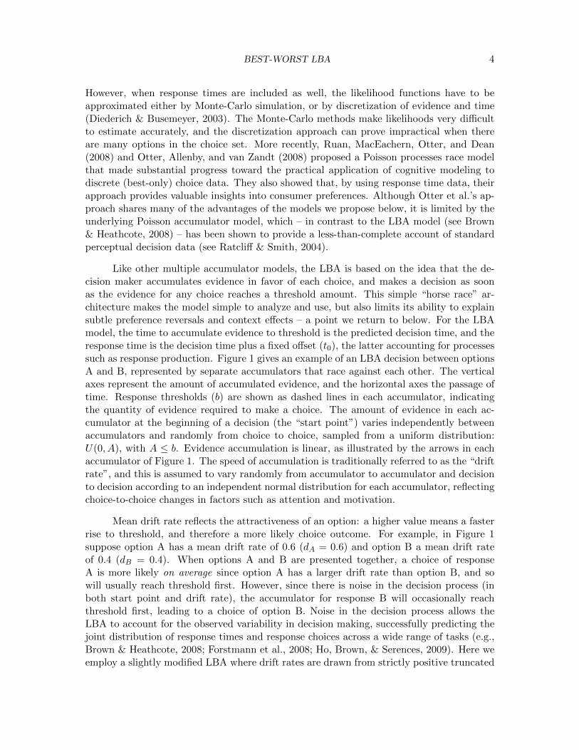
Like other multiple accumulator models, the LBA is based on the idea that the de-cision maker accumulates evidence in favor of each choice, and makes a decision as soonas the evidence for any choice reaches a threshold amount. This simple “horse race” ar-chitecture makes the model simple to analyze and use, but also limits its ability to explainsubtle preference reversals and context effects – a point we return to below. For the LBAmodel, the time to accumulate evidence to threshold is the predicted decision time, and theresponse time is the decision time plus a fixed offset (t0), the latter accounting for processessuch as response production. Figure 1 gives an example of an LBA decision between optionsA and B, represented by separate accumulators that race against each other. The verticalaxes represent the amount of accumulated evidence, and the horizontal axes the passage oftime. Response thresholds (b) are shown as dashed lines in each accumulator, indicatingthe quantity of evidence required to make a choice. The amount of evidence in each ac-cumulator at the beginning of a decision (the “start point”) varies independently betweenaccumulators and randomly from choice to choice, sampled from a uniform distribution:U(0, A), with A ≤ b. Evidence accumulation is linear, as illustrated by the arrows in eachaccumulator of Figure 1. The speed of accumulation is traditionally referred to as the “driftrate”, and this is assumed to vary randomly from accumulator to accumulator and decisionto decision according to an independent normal distribution for each accumulator, reflectingchoice-to-choice changes in factors such as attention and motivation.
Mean drift rate reflects the attractiveness of an option: a higher value means a fasterrise to threshold, and therefore a more likely choice outcome. For example, in Figure 1suppose option A has a mean drift rate of 0.6 (dA = 0.6) and option B a mean drift rateof 0.4 (dB = 0.4). When options A and B are presented together, a choice of responseA is more likely on average since option A has a larger drift rate than option B, and sowill usually reach threshold first. However, since there is noise in the decision process (inboth start point and drift rate), the accumulator for response B will occasionally reachthreshold first, leading to a choice of option B. Noise in the decision process allows theLBA to account for the observed variability in decision making, successfully predicting thejoint distribution of response times and response choices across a wide range of tasks (e.g.,Brown & Heathcote, 2008; Forstmann et al., 2008; Ho, Brown, & Serences, 2009). Here weemploy a slightly modified LBA where drift rates are drawn from strictly positive truncated

BEST-WORST LBA 5
Response A Response B
Decision Time
Start Point
Response Threshold
Drift Rate
Racing LBA Accumulators
NOISE PROCESSES: Start Point is a
i ~ Uniform(0,A)
Drift Rate is di ~ Normal (d,s)
Drift rates vary randomly from trial to trial (normal distribution).
Start points vary randomly from trial to trial (uniform distribution).
Figure 1. Illustrative example of the decision processes of the LBA. See main text for full details.
normal distributions (for details, see Heathcote & Love, 2012).3
Horse Race Models for Best-Worst Choice
We used the modified LBA to create three different models for best-worst scaling,derived from previously-applied random utility models of choice (see, e.g., Marley & Lou-viere, 2005). Each variant involves a race among accumulators representing the competingchoices. In the first, which we refer to as the ranking model, there is one race, with the first(respectively, last) accumulator to reach threshold associated with the best (respectively,worst) choice. The second variant, the sequential model, has two races that occur in se-quence; the winner of the first race determines the best response, and, omitting the winnerof the first race, the winner of the second race determines the worst response; we constraineach drift rate for the second race to be the inverse of the corresponding rate in the first race.The third variant, the enumerated model, assumes a single race between accumulators thatrepresent each possible pair of best and worst choices (e.g., 12 accumulators for 4 options).For a best-worst pair (p, q), p 6= q, the drift rate is the ratio d(p)/d(q) of the drift rate for pversus the drift rate for q. Our later fits to data show that the estimated drift rate d for anoption is, effectively, equal to the exponential of the estimated utility u for that option in thecorresponding MNL model. These are not the only plausible accumulator-based best-worstmodels. For example, best-worst choice might be modeled by two simultaneous races drivenby utilities and disutilities, respectively. However we consider these models because theycorrespond to the frameworks adopted by the marginal and paired-conditional (“maxdiff”)random utility models most commonly used to analyze best-worst scaling data (Marley &
3The normal truncation requires the density and cumulative density expressions for individual accumula-tors in Brown and Heathcote (2008) (Equations 1 and 2) to be divided by the area of the truncated normal,Φ(−d/s).

BEST-WORST LBA 6
Louviere, 2005).
General Framework
We now present the LBA-based models, by developing equations for the predictedchoice probabilities and response times (omitting fixed offset times for processes like motorproduction). To begin the notation, let S with |S| ≥ 2 denote the set of potentially availableoptions, and let X ⊆ S be a finite subset of options that are available on a single choiceoccasion. Assume there is a common threshold b across all options in the set of availableoptions X. For z ∈ S and p, q ∈ S, p 6= q, there are: a drift rate d(z); independentrandom variables U z , Up,q uniformly distributed on [0, A] for some 0 ≤ A ≤ b; andindependent normal random variables Dz and Dp,q with mean 0 and standard deviations. For best choices, the drift rate variable for option z is then given by trunc(Dz + d(z))where the truncation is to positive values, and for worst choices, the drift rate variable foroption z is then given by trunc(Dz + 1/d(z)), again with the truncation to positive values.Similarly, the drift rate variable for the best-worst pair p, q is then given by trunc(Dp,q +d(p)/d(q)). For best choices, the probability density function (PDF) of finishing times forthe accumulator for option z ∈ X at time t, denoted bX(z, t), is given by
bz(t) = Pr
(b−U z
trunc(Dz + d(z))= t
),
with cumulative density function (CDF)
Bz(t) = Pr
(b−U z
trunc(Dz + d(z))≤ t).
We denote the corresponding PDF and CDF for worst choice by wz(t) and Wz(t),which are given by replacing d(z) with 1/d(z) in the above formulae. For best-worst choicethey are bw(p,q)(t) and BW(p,q)(t) with d(p)/d(q) replacing d(z) in the above formulae.Expressions given in Brown and Heathcote (2008) can be used to derive easily computedexpressions for these PDFs and CDFs under the above assumptions, and using drift ratedistributions truncated to positive values as described in Heathcote and Love (2012). Then,given the assumption that the accumulators are independent – that is, each accumulatorhas independent samples of the start point and drift rate variability – it is simple to specifylikelihoods conditional on response choices and response times. These likelihoods for eachof the three best-worst LBA models are shown in the next three sub-sections.
When fitting data without response times, we made the simplifying assumptions thats = 1, b = 1 and A = 0, as these parameters are only constrained by latency data. Evenin response time applications, fixing s in this way is common. Estimation of b can accom-modate variations in response-bias and overall response speed, but without response timedata, speed is irrelevant and response-bias effects can be absorbed in drift rate estimates.The relative sizes of A and b are important in accounting for differences in accuracy anddecision speed that occur when response speed is emphasized at the expense of accuracy, orvice versa (Brown & Heathcote, 2008; Ratcliff & Rouder, 1998). Our setting here (A = 0)is consistent with extremely careful responding. We also tried a less extreme setting (b = 2and A = 1) with essentially equivalent results.

BEST-WORST LBA 7
Ranking Model
The ranking model is arguably the simplest way to model best-worst choice with arace. For a choice among n options it assumes a race between n accumulators with driftrates d(z). The best option is associated with the first accumulator to reach threshold andthe worst option with the last accumulator to reach threshold, as shown in the upper row ofFigure 2. To link the models to data requires an expression for the probability of choosinga particular best-worst pair for each possible choice set, X, given model parameters. ThePDF for a choice of option x as the best at time t, and option y as the worst at time r,where r > t, bwX(x, t; y, r), is given by Equation 1 shown in Figure 2, for x, y ∈ X, x 6= y.Equation 1 calculates the product of the probabilities of the “best” accumulator finishingat time t, the “worst” accumulator finishing at time r > t, and all the other accumulatorsfinishing at times between t and r. Since the data sets do not include response times, wecalculate the marginal probability BWX(x, y) of the selection of this best-worst choice pair,by integrating over the unobserved response times (t and r) – see Equation 2 in Figure 2.
Ranking
Sequential
Enumerated
bwX(x, t; y, r) = bx(t) · by(r)∏
(p,q)∈X×X−(x,y)p $=q
(Bp(r)−Bq(t)).
BWX(x, y) =
∫ ∞
0
∫ ∞
tbwx,y(x, t; y, r) dr dt.
BWX(x, y) =
∫ ∞
0bw(x,y)(t)
∏
(p,q)∈X×X−(x,y)p %=q
(1−BW(p,q)(t)) dt.
(1)
(2)
(3)
(4)
(5)
Threshold (b)
Decision time
Best
(fastest)
Worst
(slowest)
Best race
Worst race
Best
(fastest)
Worst
(fastest)
Accumulator 1
x = Best
y = Worst
(fastest) !
Accumulator 2 Accumulator n(n-1)
BX(x) =
∫ ∞
0bx(t)
∏
z∈X−{x}(1−Bz(t)) dt.
WX−{x}(y) =∫ ∞
0wy(r)
∏
z∈X−{x,y}(1−Wz(r)) dr.
Figure 2. Illustrative example of the decision processes of the ranking, sequential and enumeratedversions of the best-worst race models and their associated formulae (upper, middle and lowers rows,respectively). See main text for full details.
The ranking model predicts that the best option is chosen before the worst option,which may not be true in data. The ranking model could also be implemented in a worst-to-best form, with the first finishing accumulator associated with the worst option and thelast finishing accumulator with the best option, and with each drift rate the inverse of the

BEST-WORST LBA 8
corresponding drift rate in the best-to-worst version. It is difficult to separate these versionsuntil we have response time data, which we return to later.
Sequential Model
The sequential race model assumes the best-worst decision process is broken intotwo separate races that occur consecutively (see middle row of Figure 2). The best raceoccurs first and selects the best option. The worst race then selects the worst option. Thesequential model could have 2× n mean drift rate parameters – one for each option in thebest race, and one for each option in the worst race. To simplify matters, we assume that,for each z ∈ S, the drift rate is d(z) in the best race and 1/d(z) in the worst race. Thisensures that desirable choices (high drift rates) are both likely to win the best race andunlikely to win the worst race. We also assume that the worst-choice race does not includethe option already chosen as best so that the same option cannot be chosen as both bestand worst.
The first accumulator to reach threshold is selected as the best option. The prob-ability for a choice of the option x as the best, BX(x), is given in Equation 3. It is theprobability density that accumulator x finishes at time t, and all the other accumulatorsfinish at times later than t, integrated over all times t > 0. The worst race is run with theaccumulators in the set X − {x}. The first accumulator to reach threshold is selected asthe worst option, but each drift rate is now the inverse of the corresponding drift rates inthe first race. The probability of a choice of the option y as the worst, WX−{x}(y), is givenin Equation 4. The joint probability for the sequential model of choosing x as the best andy as the worst, BWX(x, y), is simply the product of Equations 3 and 4.
Clearly, a corresponding model is easily developed where the worst race occurs firstand selects the worst option, and the best race occurs second and selects the best option.
Enumerated Model
The enumerated model assumes a race between each possible best-worst pair in thechoice set. This is analogous to the paired conditional (also called “maxdiff”) random utilitymodel (Marley & Louviere, 2005). For a choice set with n options, the model assumes arace between n× (n− 1) accumulators. This model predicts a single decision time for bothresponses. The probability of choosing x as best and y 6= x as worst for this model is shownin Equation 5.
For a choice set with n options, the enumerated model could have n × (n − 1) driftrate parameters. However, we simplified the enumerated model in a similar way to thesequential model, by again defining the desirability of options by their drift rates, and theundesirability of options by the inverse of their drift rates. In particular, we estimateda single drift rate parameter d(z) for each choice option z, and set the drift rate for theaccumulator corresponding to the option pair (p, q) to the ratio d(p)/d(q).
Estimating Model Parameters from Data
We fit the three race models to two best-worst choice data sets, one about patients’preferences for dermatology appointments (Coast et al., 2006), and the second about pref-erences for mobile phones (Marley & Pihlens, 2012). In both data sets response times were

BEST-WORST LBA 9
unavailable (i.e., not recorded) and the data structure was “long but narrow” – large samplesizes with relatively few data points per participant – which is standard in discrete choiceapplications. Coast et al.’s data investigated preferences for different aspects of dermato-logical secondary care services. Four key attributes were identified as relevant to patientexperiences, one of which had four levels, with the remaining three having two levels each(see Table 1). We denote each attribute/level combination (henceforth, “attribute level”)with two digits, shown in parentheses in the right column of Table 1. The first digit refersto the attribute and the second digit to its level: for example, attribute level “32” refers tolevel 2 of attribute number 3. For all four attributes, the larger the second digit (i.e., levelof the attribute) the more favorable the level of the attribute.
Table 1: The four attributes and their levels from Coast et al. (2006). The values in parenthesesindicate the coding used in Figure 3 below.
Attribute Attribute levels
Waiting time (1) Three months (11)Two months (12)One month (13)This week (14)
Doctor expertise (2) The specialist has been treating skin complaintspart-time for 1-2 years (21).The specialist is in a team led by an expert whohas been treating skin complaints full-time forat least 5 years (22).
Convenience of appointment (3) Getting to the appointment will be difficult andtime consuming (31).Getting to the appointment will be quick andeasy (32).
Thoroughness of consultation (4) The consultation will not be as thorough as youwould like (41).The consultation will be as thorough as youwould like (42).
Participants were given a description of a dermatological appointment that includeda single level from each attribute, and asked to indicate the best and the worst attributelevel. For example, on one choice occasion, a participant might be told that an upcomingappointment is: two months away (12); with a highly specialized doctor (22); at an incon-venient location (31) and not very thorough (41). They would then be asked to choose thebest and worst thing about this appointment. The same 16 scenarios were presented toeach participant in the study, and were chosen using design methodology that enabled allmain effects to be estimated. Below we compare the parameters estimated from the racemodels to parameters of the MNL models for Coast et al.’s (2006) choice data reported byFlynn et al. (2008).
Marley and Pihlens (2012) examined preferences for various features of mobile phonesamong 465 Australian pre-paid mobile phone users in December 2007. There were nine

BEST-WORST LBA 10
mobile phone attributes with a combined 38 attribute levels, described in Table 2. Thevalues in parentheses in Table 2 code attribute levels in a manner similar to Table 1, thoughnot all attributes have a natural preference order. Each respondent completed the same 32choice sets with four profiles per set. Each phone profile was made up of one level from eachof the nine attributes. Participants were asked to provide a full rank order of each choiceset by first selecting the best profile, then the worst profile from the remaining three, andfinally the best profile from the remaining two. Here, we restrict our analyses to choices ofthe best and the worst profile in each choice set.
Parameter Constraints
A natural scaling property of the LBA model, parallel to MNL models, is that thedrift rate distributions for competing choices can be multiplied by an arbitrary scale factorwithout altering predicted choice probabilities – although response time predictions will beaffected. We employed a modified LBA model, with truncated normal drift rate distribu-tions. In this version, multiplying the drift rate parameters does not simply multiply alldistributions. Rather, the distribution shape is altered because the amount of truncationchanges depending on how far the mean of the distribution falls from zero. For this rea-son, the scaling property holds only approximately for the truncated-normal LBA, and theapproximation depends on the size of the drift rate parameters.
For the mobile phone data, there were 38 different attribute levels, and the approxi-mation to the regular scaling property held well enough that we were able to constrain theproduct of the estimated drift rates across the attribute levels to one, for each attribute.This results in 29 free drift rate parameters, and mirrors Marley and Pihlens’ (2012) con-straints on their MNL model parameters. The dermatology data involved more extremechoice probabilities, and so smaller drift rates for some attributes. Therefore, we were notable to exploit the usual scaling property, and we imposed no constraints: there were 10attribute levels, and we estimated 10 free drift rates. We note that this freedom allows us,theoretically, to separately estimate mean utility parameters and the associated varianceparameters, which may prove useful in future research (Flynn, Louviere, Peters, & Coast,2010).
Model Fit
We aggregated the data across participants; thus, for each choice set in the design,we fit a single set of choice probabilities. We used two methods to evaluate the fit ofthe race models to data. The first compared drift rate estimates to corresponding randomutility models regression coefficients reported by Flynn et al. (2008) and Marley and Pihlens(2012). In this comparison we take the logarithm of the drift rates, bringing them onto thesame unbounded domain as the utility parameters. Secondly, we examined the race models’goodness of fit by comparing observed and predicted best-worst choice proportions. For eachchoice set, observed best-worst choice proportions were calculated by dividing the numberof times a particular best-worst pair was selected across participants by how many timesthat particular choice set was presented across participants.

BEST-WORST LBA 11
Results
Coast et al.’s (2006) Dermatology Data
Flynn et al. (2008) analyzed Coast et al.’s (2006) data using a paired model conditionallogit regression, adjusted for covariates.4 Flynn et al.’s regression coefficients were expressedas treatment-coded linear model terms (main effects for attributes, plus treatment effectsfor each level). For example, Flynn et al. found that the main effect for the “convenience”attribute was 0.715 with a treatment effect of 1.501 for the “very convenient” level (Table4; Flynn et al.). For ease of comparison, we expressed the estimated drift rate parametersfrom the LBA models in this same coding. We referenced all parameters against the zeropoint defined by the waiting time attribute, by subtracting the mean drift rate for thisattribute from all drift rates. We then calculated the main effect for each attribute asthe mean drift rate for that attribute, and calculated treatment effects for each attributelevel by subtracting the main effects. These calculations are independent of the parameterestimation procedure and were done solely to facilitate comparison with Flynn et al.’sresults.
The upper row of Figure 3 compares the log drift rates estimated from the three racemodels against the corresponding parameters from Flynn et al.’s (2008) fit of the maxdiff(MNL) model; Appendix A gives the form of that model. The four main effect estimatesare shown as bold faced single digits, and treatment effects as regular faced double digits,using the notation from Table 1. For all three model variants, there was an almost perfectlinear relationship between log drift rates estimated for the race model and the parametersfor the corresponding MNL model.
All of the race models provided an excellent fit to the dermatology data, as shownin the lower row of Figure 3. In those plots, a perfect fit would have all the points fallingalong the diagonal line. For all models there was close agreement between observed andpredicted values, with all R2’s above .9. The root-mean-squared difference between observedand predicted response probabilities was 5.4%, 5.1% and 5.3% for the ranking, sequentialand enumerated models, respectively. The corresponding log-likelihood values were −1379,−1406 and −1381, respectively, providing little basis to select between LBA models in thisanalysis. Flynn et al.’s (2008) marginal model conditional logit analysis, which has thesame number of free parameters as our LBA models, produced a log-pseudolikelihood of-1944 suggesting that the LBA provides a better fit to this data.
Marley & Pihlens’ (2012) Mobile Phone Data
Marley and Pihlens (2012) analyzed their full rank data using a repeated maxdiff(MNL) model;5 Appendix A gives the form of that maxdiff model for the first (best) and last(worst) options in those rank orders. We compare the log drift rate parameter estimatesfrom our race models for those first (best) and last (worst) choices against Marley andPihlens’ utility parameter estimates. The upper row of Figure 4 plots the estimated log
4Flynn et al. (2008) also performed a paired model conditional logit regression (without covariates) anda marginal model conditional logit analysis. The regression coefficients did not differ much across theseanalyses, and so we ignore those, for brevity.
5Marley and Pihlens (2012) also analyzed their data using other variants of the MNL framework, withlittle difference to the estimated coefficients. Again, for brevity, we show just the main analyses.

BEST-WORST LBA 12
11
12
13
14
21
22
31
32
41
42
1
23
4
R2
= .929
RankingE
stim
ate
d ‘R
egre
ssio
n C
oeffic
ients
’fr
om
Log L
BA
Dri
ft R
ate
s
−1.5
−1
−.5
0
.5
1
1.5
−4 −3 −2 −1 0 1 2 3 4
11
12
13
14
21
22
31
32
41
42
1
2
34
R2
= .978
Sequential
Regression Coefficients from Data
−4 −3 −2 −1 0 1 2 3 4
1112
13
14
21
22
31
32
41
42
1
2
34
R2
= .989
Enumerated
−4 −3 −2 −1 0 1 2 3 4
0 .1 .2 .3 .4 .5 .6 .7
Best−
Wors
t C
hoic
e P
robabili
ties fro
m L
BA
0
.1
.2
.3
.4
.5
.6
.7 R2
= .907
0 .1 .2 .3 .4 .5 .6 .7
Best−Worst Choice Proportions from Data
R2
= .916
0 .1 .2 .3 .4 .5 .6 .7
R2
= .908
Figure 3. Log drift rate parameter estimates (upper row), plotted against Flynn et al.’s (2008)utility estimates, and goodness of fit (lower row) of the ranking, sequential and enumerated racemodels (columns) to Coast et al.’s (2006) data. In the upper row, bold face single digits representmain effects, double digits represent attribute levels, using the notation from Table 1. In the lowerrow, the x-axes display best-worst choice proportions from data, the y-axes display predicted best-worst choice probabilities from the estimated race model. The diagonal lines show a perfect fit.
drift rates from the race models against the regression coefficients from Marley and Pihlens’maxdiff model. There was again a nearly perfect linear relationship between log drift ratesestimated for the race model and regression coefficients.
To further demonstrate the strength of the linear relationship between drift ratesand utility estimates, we re-present the parameter values for the sequential model shown inFigure 4 separately for each attribute, in Figure 5. Figure 5 clearly illustrates the almostperfect correspondence between the rank ordering on drift rates and the rank ordering onregression coefficients. Not only do the drift rates preserve the ordering, but also differencesin magnitude between levels of each attribute. For example, the price attribute, shown inthe upper right panel of Figure 5, demonstrates that people have the strongest preference forthe cheapest phones ($49) and the weakest preference for the most expensive ones ($249).However, the difference in utility (regression coefficients) is much greater between someadjacent levels than others (e.g., moving from the third to the forth level, $199 to $249).

BEST-WORST LBA 13
s1
s2
s3
s4s5
s6
s7
s8b1
b2
b3b4
p1
p2p3
p4
c1
c2c3
c4
w1
w2
w3w4
v1
v2v3v4
i1
i2
m1
m2
m3
m4
r1
r2r3
r4
R2
= .979
Ranking
Log L
BA
Dri
ft R
ate
s
−.3
−.2
−.1
0
.1
.2
s − styleb − brandp − pricec − cameraw − wirelessv − videoi − webm − musicr − memory
−.3 −.2 −.1 0 .1 .2
s1s2
s3
s4s5
s6
s7s8
b1
b2
b3b4
p1
p2
p3
p4
c1
c2
c3
c4
w1
w2w3
w4
v1
v2v3v4
i1
i2
m1
m2
m3
m4
r1
r2r3
r4
R2
= .991
Sequential
Regression Coefficients from Data
−.3 −.2 −.1 0 .1 .2
s1s2s3
s4s5s6
s7s8b1
b2
b3b4
p1
p2p3
p4
c1
c2c3
c4
w1
w2w3
w4
v1
v2v3v4
i1
i2
m1
m2
m3
m4
r1
r2r3r4
R2
= .997
Enumerated
−.3 −.2 −.1 0 .1 .2
0 .1 .2 .3
Best−
Wors
t C
hoic
e P
robabili
ties fro
m L
BA
0
.1
.2
.3
R2
= .574
0 .1 .2 .3
Best−Worst Choice Proportions from Data
R2
= .594
0 .1 .2 .3
R2
= .592
Figure 4. Log drift rate parameter estimates (upper row), plotted against Marley and Pihlens’(2012) regression coefficients, and goodness of fit (lower row) of the ranking, sequential and enu-merated race models (left, middle and right columns, respectively) to Marley and Pihlens’ mobilephone data. In the upper row, each point represents an attribute level, where the letter indicatesthe attribute and the number indicates the level of the attribute, as in Table 2. In the lower row,the x-axes display best-worst choice proportions from data, the y-axes display predicted best-worstchoice probabilities from the estimated race model, and the diagonal lines represent a perfect fit.
Such a difference in magnitude also occurred in, for instance, the camera attribute, wherea phone with no camera (level 1) was much less desirable than any phone with a camera(levels 2, 3 and 4). In all cases the estimated drift rates were sensitive to such differences inmagnitude as well as the rank ordering. Sensitivity to these important outcome measures(ranking and magnitude) suggests the race models may be useful for measurement purposes.
We assessed the goodness of fit of each model by comparing observed and predictedproportions, shown in the lower half of Figure 4. As with the dermatology data, there wasexcellent agreement, with 3.2% root-mean-squared prediction error for all three models.Although the goodness-of-fit appears poorer in Figure 4 compared to Figure 3, this isactually due to differences in the scale of the axes across figures. The R2’s were smallerthan for the dermatology data (though all are > .57), reflecting greater inter-individualvariability in choices. To compare with the goodness of fit for the MNL models reported by

BEST-WORST LBA 14
Marley and Pihlens (2012), we calculated McFadden’s ρ2 measure. McFadden’s ρ2 measuresthe fit of a full model with respect to the null model (all parameters equal to 1), defined as
ρ2 = 1− ln L(Mfull)
ln L(Mnull), where ln L(Mfull) and ln L(Mnull) refer to the estimated log-likelihood
of the full and null models, respectively. This showed almost identical results for the racemodels (ranking ρ2 = .245, sequential ρ2 = .246, and enumerated ρ2 = .246) as the MNLmodels (best, then worst, ρ2 = .244, and maxdiff ρ2 = .245).
−.2
−.1
0
.1
.2Style
1 − Flip2 − Straight3 − Slide4 − Swivel
5 − Touch6 − PDA half7 − PDA full8 − PDA touch
12345
67 8
Brand
1 − A2 − B3 − C4 − D
1
2
34
Price
1 − $492 − $1293 − $1994 − $249
1
23
4
Log L
BA
Dri
ft R
ate
s
−.2
−.1
0
.1
.2Camera
1 − None2 − 2mp3 − 3mp4 − 5mp
1
23
4
Wireless
1 − No BlueT/WiFi2 − WiFi3 − BlueT4 − BlueT & WiFi
1
234
Video
1 − None2 − 15min3 − 1hr4 − >1hr
1
234
−.2 −.1 0 .1 .2
−.2
−.1
0
.1
.2Web
1 − Access2 − None
1
2
Regression Coefficients from Data
−.2 −.1 0 .1 .2
Music
1 − None2 − MP33 − FM4 − MP3 & FM
1
2
3
4
−.2 −.1 0 .1 .2
Memory
1 − 64MB2 − 512MB3 − 2GB4 − 4GB
1
234
Figure 5. Fit of the sequential race model to Marley and Pihlens’ (2012) mobile phone data, shownseparately for each attribute. Log drift rates are plotted against Marley and Pihlens’ regressioncoefficients. Each panel represents a different attribute. The numbers inside the nine panels representeach attribute level. The black lines in each panel represent the regression line fit to the sequentialrace model log drift rates and Marley and Pihlens’ regression coefficients shown in the middle panelof the upper row in Figure 4. The dashed horizontal and vertical lines represent zero-referencepoints.
As a final comparison with existing MNL models for best-worst data, we comparedthe race models’ drift rate parameters against “best minus worst scores” calculated from thedata.6 As with similar analyses in the literature (Finn & Louviere, 1992; Goodman, 2009;
6These scores are normalized differences between the number of “best” responses and “worst” responses

BEST-WORST LBA 15
Mueller Loose & Lockshin, 2013), for both data sets the agreement between the best minusworst scores and the drift rates was just as strong as the relationship between drift rates andregression coefficients, reinforcing the current consensus that the best minus worst scoresare a simple, but useful, way to describe data. Theoretical properties of these scores for themaxdiff model of best-worst choice are stated and proved in Flynn and Marley (submitted),Marley and Islam (2012) and Marley and Pihlens (2012).
Discussion
The MNL-inspired LBA model variants we proposed are all capable of fitting the der-matology and mobile phone data sets at least as well as the standard MNL choice models.Although the three models make different assumptions about the cognitive processes under-lying best-worst choices all fit the data equally well, making them difficult to distinguish onthe basis of choices alone. Response time data have the potential to tease the models apart –for example, the ranking LBA model makes the strong prediction that “best” responses willalways be faster than “worst” responses. Testing such predictions against data can betterinform investigations into the cognitive processes underlying preferences, paralleling similardevelopments in the understanding of single-attribute perceptual decisions (e.g., see Ratcliff& Smith, 2004) and best-only decisions about multi-attribute stimuli (Otter et al., 2008;Ruan et al., 2008). This illustrates the potential benefits that arise from using cognitiveprocess-based models (such as accumulator models) for both choice and response time.
In the next section we demonstrate that a best-worst scaling task that incorporatesresponse time measurement can aid discrimination between the LBA variants we have pro-posed. We show that the three LBA variants introduced above, derived from analogousMNL models, are inconsistent with the response time data from a perceptual judgmenttask. We propose a modification to the sequential LBA model that naturally accountsfor the response latency data, demonstrating that response times provide added benefit tobest-worst scaling.
Response Times in Best-Worst Scaling
The lack of latency data is commonplace in the applied discrete choice literature.Traditionally, it has not been thought necessary to record response latency as it has notbeen demonstrated how such measurement might usefully be included in analyses (thoughfor recent progress see, e.g., Dellaert, Donkers, & van Soest, 2012; Haaijer, Kamakura, &Wedel, 2000; Otter et al., 2008; Ruan et al., 2008). Race models provide a natural accountof decision times in best-worst scaling, so we examined the response time predictions of thepreviously proposed LBA models against data from a new experiment.
The ranking, sequential and enumerated race models make unique predictions aboutthe pattern of predicted response times. For example, the ranking and sequential modelspredict that best responses always occur prior to worst responses. Alternatively, the twomodels could be instantiated in a worst-to-best fashion, in which case they predict worstresponses always occur before best responses. However, compared to the ranking model, thesequential model predicts a faster distribution of worst responses – because in the sequentialmodel, an entirely new race must be run after the “best” response is issued. If the data
elicited by each attribute level.

BEST-WORST LBA 16
exhibit a mixture of response ordering – sometimes the “best” before “worst”, and viceversa – then we have evidence against the assumptions of these two models, at least fortheir strict interpretation. We discuss below implications of response order patterns indata, and the possible inclusion of a mixture process that permits variability in the orderof the races (i.e., the ranking model might sometimes occur in a worst-to-best manner andsometimes in a best-to-worst manner, or the sequential model might occur in a worst-then-best order and sometimes in a best-then-worst order). The enumerated model also makesstrong predictions about response times: best and worst choices should differ only by anoffset time due to motor processes, since the single enumerated race provides both thebest and worst responses. Consequently, the enumerated model predicts that experimentalmanipulations, such as choice difficulty or choice set size, should not influence the timeinterval between the best and worst responses.
As a first target for investigating models of response times in best-worst scaling ex-periments we chose to use a simple perceptual judgment task rather than a traditionalconsumer choice task. Perceptual choices permit the collection of many more trials thancomplex consumer judgments. This enabled us to collect a large number of trials per par-ticipant, providing data that could more easily support a finer-grained analysis of responsetime distributions and fitting models to individual participant data. In addition, perceptualtasks permit precise stimulus control that allow testing of, for example, enumerated modelpredictions such as the absence of choice difficulty effects on inter-response times. We leaveto future research the investigation of response time data from more typical multi-attributediscrete choice applications, such as the dermatology and mobile phone examples examinedin the first section.
Experiment
We used a modified version of Trueblood, Brown, Heathcote, and Busemeyer’s (inpress) area judgment task. At each trial participants were presented with four rectanglesof different sizes, and they were asked to select the rectangle with the largest area (i.e., ananalogue to a “best” choice) and the smallest area (i.e., an analogue to a “worst” choice).
Participants
Twenty-six first year psychology students from the University of Newcastle partici-pated in the experiment online in exchange for course credit.
Materials and Methods
The perceptual stimuli were adapted from Trueblood et al. (in press), where partic-ipants were asked to judge the area of black shaded rectangles presented on a computerdisplay. We factorially crossed three widths with three heights to generate nine uniquerectangles, with widths, heights and areas given in Table 3. The area of the rectangles atthe extreme ends of the stimulus set were easily differentiable (e.g., 6050 from 8911), butthose in the middle of the stimulus set were much more difficult (e.g., 8107 from 8113).
On each trial, four rectangles were randomly sampled, without replacement, from theset of nine rectangles. The stimuli were presented in a horizontal row in the center of the

BEST-WORST LBA 17
screen, as shown in Figure 6. All rectangles were subject to a random vertical offset between±25 pixels, to prevent the use of alignment cues to judge height.
Figure 6. Illustrative example of a trial in the area judgment task. Note that if a participantselected, say, “Largest 1” as the rectangle with the largest area, then the option “Smallest 1” wasmade unavailable for selection.
Each participant chose the rectangle judged to have the largest area, and a differentone with the smallest area. All responses were recorded with a mouse click and couldbe provided in either order: largest-then-smallest, or smallest-then-largest. We restrictedparticipants from providing the same rectangle as both the largest and smallest option, byremoving the option selected first as a possibility for the second response. On each trialwe recorded the rectangle chosen as largest and the latency to make the choice, and therectangle chosen as smallest and the time to make that choice. Participants completed 600trials each, across three blocks.
Results
We excluded trials with outlying responses that were unusually fast or slow, definedas faster than .5 seconds or slower than 25 seconds. We also excluded two participants whoeach had more than 10% of their trials marked as outliers. Of the remaining participants’data, outliers represented only 0.9% of total trials.
We first report the proportion of correct classifications – correct selection of the largest(resp., smallest) rectangle in the stimulus display. We follow this analysis by consideringthe effect of response order – whether participants responded in a largest-then-smallest, orsmallest-then-largest, manner – on both choice proportion and response latency data.
Correct Classifications
Our first step in analysis was to determine whether the area judgment manipulationhad a reliable effect on performance. The left and middle panels of Figure 7 display the

BEST-WORST LBA 18
proportion of correct responses for largest (resp., smallest) judgments as a function of choicedifficulty. We operationalized difficulty as the difference in area between the largest (resp.,smallest) and second largest (resp., second smallest) rectangle presented at each trial, whichwe refer to as the max-vs-next (resp., min-vs-next) difference. A small max-vs-next (resp.,min-vs-next) difference in area makes it difficult to resolve which is the largest (resp.,smallest) rectangle.
0 500 1000 1500 2000
.3
.4
.5
.6
.7
.8
.9
1
Max−vs−Next Difference (pixels)
Me
an P
rop
ort
ion
Corr
ect
0 500 1000 1500 2000
Min−vs−Next Difference (pixels)
Data
Cumulative normalpsychophysical function:
Max−vs−Next Mean = 54, SD = 740
Min−vs−Next Mean = 121, SD = 739
Figure 7. The left panel shows the proportion of times that the rectangle chosen as best was thelargest rectangle (i.e., correct choice) as a function of the difference in area between the largest andsecond largest rectangles in the display (in pixels). The middle panel shows the proportion of timesthat the rectangle chosen as worst was the smallest rectangle as a function of the difference in areabetween the smallest and second smallest rectangles in the display. The overlaid lines represents thebest fitting cumulative normal psychophysical functions, fit separately to both panels, with legendshown in the right panel.
Performance was well above chance even for the smallest max-vs-next and min-vs-next differences (6 and 11 pixels, respectively), yielding 45% and 50% correct selectionsof the largest and smallest rectangles in the display, respectively (chance performance is25%). As expected, when the max-vs-next and min-vs-next difference increased, so to didthe proportion of correct responses. We have separately overlaid on the max-vs-next andmin-vs-next difference scores the best-fitting cumulative normal psychophysical functions.The good fit is consistent with the notion that participants’ decisions were sensitive to anoisy internal representation of area.
Response Order Effects
To connect the following model and data with earlier material, we refer to best (resp.,worst) rather than largest (resp., smallest). There was considerable variability across partic-ipants in the proportion of best-before-worst versus worst-before-best responses (Figure 8),ranging from almost completely worst-first to almost completely best-first. Over partic-ipants, the majority of first responses were for the best option (M = .73), which wassignificantly different from chance according to one sample t-test (i.e., test against µ = .5),

BEST-WORST LBA 19
t(23) = 3.18, p = .004. These patterns suggest that models which strictly impose a singleresponse ordering, such as the ranking and sequential models, require modification.
Participants Sorted on Data
0
.2
.4
.6
.8
1
Pro
po
rtio
n o
f B
est−
First
Re
sp
on
se
s
Data
Model
Figure 8. Proportion of trials on which the best response was made before the worst response,shown separately for each participant. Circular symbols and crosses represent data and predictionsof the simultaneous race model, respectively. Error bars represent the standard error of a binomialproportion, according to the formula: se(p) =
√p(1− p)/n, where p is the proportion of best-first
choices in data and n is the number of trials. The dashed horizontal line represents the meanproportion of best-first responses across participants.
We next examined whether choice difficulty influenced response order. We definedthe difficulty of best and worst choices respectively using the max-vs-next and min-vs-nextcriteria described above, but we collapsed these into three exhaustive difficulty categories:hard (less than 250 pixels), medium (500–1000 pixels), and easy (greater than 1250 pixels;no difference scores fell between 250–500 or 1000-1250 pixels). The mean proportion of best-first responses reliably decreased as the discrimination of the largest rectangle became moredifficult, F (1.4, 31.9) = 4.07, p = .04, using Greenhouse-Geisser adjusted degrees of freedom(all subsequent ANOVAs also report Greenhouse-Geisser adjusted degrees of freedom). Thiseffect suggests that when there is an easy-to-see largest rectangle, that response was likelyto be made first: easy M = .739 (within-subjects standard error = .006), medium M = .726(.003) and hard M = .719 (.006). The analogous result was observed for worst-first choices,but larger in effect size – an easy-to-see smallest rectangle made a worst-first response morelikely, F (1.6, 35.7) = 10.03, p < .001; easy M = .289 (.006), medium M = .275 (.004) andhard M = .256 (.006).
We also examined the effect of choice difficulty on the time interval between the firstand second responses – the inter-response time. For each participant we calculated theaverage inter-response time for best-first trials as a function of the difficulty of the worst(second) response (easy, medium, difficult), and for worst-first trials as a function of thedifficulty of the best (second) response. As the second judgment became more difficult,the latency between the first and second responses increased, approximately half a second

BEST-WORST LBA 20
across the three difficulty levels, F (1.2, 24.8) = 10.81, p = .002;7 easy M = 1.51s (.12),medium M = 1.75s (.08) and hard M = 1.95s (.109).
Discussion
Data from the best-worst perceptual choice experiment exhibited three effects relevantto testing the models: large differences between participants in the preference for best-then-worst versus worst-then-best responding; changes in the proportion of best-first and worst-first responding as a function of choice difficulty; and changes in inter-response times dueto choice difficulty. These effects are inconsistent with all three MNL-derived race modelsin their original forms. Firstly, the three models cannot accommodate within-participant,across-trial variability in best-first or worst-first responding. They might be able to accountfor the response order effects through the addition of a mixture process. On a certainproportion of trials, defined by a new parameter, the ranking race or the sequential racescould be run in reverse order, or the enumerated model could execute its responses inopposite orders (Marley & Louviere, 2005, considered such mixture models for best-then-worst and worst-then-best choice).
The mixture approach adds a layer of complexity to the model – an extra componentoutside the choice process itself – which is unsatisfying. Putting that objection aside, thesechanges would not be able to account for the effect of choice difficulty on the proportion ofbest- and worst-first responses, or on the inter-response times, because the mixture processis independent of the choice process. For these reasons we do not explore the fit to responsetime data of the ranking, sequential or enumerated models when augmented with a mixtureprocess. Instead we propose a modification to the sequential model, preserving the ideathat there are separate best-choice and worst-choice races, but assuming that they occursimultaneously rather than sequentially.
The Simultaneous Model
The simultaneous model makes predictions consistent with the choice and responsetime patterns observed in data. Where the sequential model assumes consecutive best, thenworst, races, the simultaneous model assumes concurrent best and worst races. The bestoption is associated with the first accumulator to reach threshold in the best race, and theworst option is associated with the first accumulator to reach threshold in the worst race.We present, and test, the simplest version of this model which allows the same option to beselected as both best and worst, which was not allowed in our experiment. The model alsoallows for vanishingly small inter-response times, which are not physically possible. Thesepredictions affect a sufficiently small proportion of decisions for our rectangle data that weneglect them here, for mathematical convenience.
The probability of a choice of the option x as best at time t and option y as worst attime r, where no constraint exists between t and r, is given as the product of the individuallikelihoods of the best and worst races,
bwX(x, t; y, r) = bx(t)∏
z∈X−{x}(1−Bz(t)) · wy(r)
∏
z∈X−{y}(1−Wz(r)).
7Data from three participants were removed from this analysis due to incomplete data in all cells.

BEST-WORST LBA 21
To calculate marginal probability BWX(x, y) from the simultaneous race model in theabsence of response time data, the individual likelihoods of the best and worst races areintegrated over all times t > 0 and r > 0, respectively. When fit in this manner to choices,only, the simultaneous model provides an account of the dermatology and mobile phone datasets equal in quality to the three LBA models described in the first section (dermatology– correspondence between MNL model regression coefficients and log estimated LBA driftrates, R2 = .97, close agreement between observed and predicted choice proportions, R2 =.92, and 5% and root-mean-squared prediction error; mobile phones – R2 = .99, R2 = .60,and 3.7%, respectively).
The simultaneous model overcomes the drawbacks of the three previous models byaccounting for all general choice and response time trends observed in data. For instance,the model is able to capture inter- and intra-individual differences in response style – thoseparticipants that prefer to respond first with the best option, or first with the worst option– by allowing separate threshold parameters for the best and worst races. For example, aparticipant who primarily responds first with the best option will be described by a lowerresponse threshold in the best race than in the worst race. This means that, on average, anaccumulator in the best race reaches threshold prior to an accumulator in the worst race.
The simultaneous race model also accounts for the effect of choice difficulty on best-and worst-first responses, via differences in drift rates across rectangles. Very easy discrim-ination of the largest rectangle tends to occur when there is a large area for one rectangle,with a correspondingly large drift rate and so a fast response and a largest-before-smallestresponse order. Similarly, the simultaneous model predicts that difficult judgments rise tothreshold more slowly than easy judgments. Therefore, irrespective of whether the best orworst race finishes first, the slower of the two races will still exhibit an effect of choice dif-ficulty on latency. Since the best and worst races are (formally) independent, by extensionthe difficulty of the slower (second) judgment will also affect the inter-response time.
Estimating Simultaneous Model Parameters from Perceptual Data
We fit the simultaneous model to individual participant data from the best-worst areajudgment task. Our methods were similar to those used previously with the multi-attributedata. We estimated nine drift rate parameters, one for each rectangle stimulus. We fit themodel twice, once where we ignored response time data (as before) and once where we usedthose data. When ignoring response times, we arbitrarily fixed A = 0, b = 1, s = 1 andt0 = 0 for the best and worst races. When fitting the model to response times, we estimateda single value of the start-point range, A, and non-decision time, t0, parameters, withseparate response thresholds for the best and worst races, bbest and bworst (we again fixeds = 1, which serves the purpose of fixing a scale for the evidence accumulation processes).Therefore, when the simultaneous model was fit to response time data it required fouradditional free parameters compared to fits to choice-only data. Regardless of the datatype – choice-only, or choices and response times – the approach to parameter optimizationwas the same: for each participant and trial we calculated the log-likelihood given modelparameters, summed across trials, and maximized. We provide code to fit the simultaneousmodel to a single participant’s data to choices and response times in the freely available Rlanguage (R Development Core Team, 2012) in the “publications” section of the authors’website at http://www.newcl.org/.

BEST-WORST LBA 22
Model Fits
Although we fit the model to data from individual participants, for ease of expositionwe primarily report the fit of the models at the aggregate level (i.e., results summed overparticipants). Unlike the previous fits, where we compared drift rate estimates to the corre-sponding random utility model regression coefficients, here we compare drift rate estimatesto the area of the rectangles to demonstrate that the model recovers sensible parameter val-ues. As above, we first assess goodness of fit by comparing observed and predicted choiceproportions. For each participant we calculated the number of times that each rectanglearea was chosen as best (resp., worst), and then normalized by the number of trials onwhich each rectangle area was presented. For the fits to response time data, we also exam-ine goodness of fit by assessing the observed and predicted distribution of best and worstresponse times at the aggregated level. To demonstrate that the model captures individualdifferences, we also present examples of model fits to individual participant response timedistributions. Finally, we compared predictions of the model to the response order data(choice proportions and response times).
Choice Proportions
The upper panels of Figure 9 plot mean estimated drift rate from the simultaneousmodel against rectangle area. Whether based on fits to choices-only or to choices andresponse times, the estimates followed a plausible pattern – mean drift rate increased asa sigmoidal function of rectangle area, which is the standard pattern in psychophysicaljudgments (e.g., Ratcliff & Rouder, 1998). There was a very strong effect of rectangle areaon mean estimated log drift rate, for the fits to choice-only, F (2.1, 49.3) = 161, p < .001,and response time, F (2.1, 48.8) = 143, p < .001, fits.
The middle and lower panels of Figure 9 show the goodness of fit of the simultaneousmodel to choice data, separately for both methods of fitting the model. Choice-only fitsprovided an excellent account of the best and worst choice proportions – both R2’s > .98and root-mean-squared difference between observed and prediction choice proportions of1.7% and 4%, respectively. When the model was forced to accommodate response times aswell as response choices, it still provided a good fit to choice proportion data: R2’s > .95and root-mean-squared prediction error of 7.1% and 7.5% for best and worst proportions,respectively. The slight reduction in goodness of fit is expected, since the latter model fitsare required to account for an additional aspect in the data (response times) – predictions ofresponse times and response choices are not independent, and the data contain measurementnoise.
Response Times
When fit to response times, the simultaneous model provides a good account of bestand worst response time distributions. We first consider group level data where we useda quantile averaging approach to analyse aggregate response time distributions. Quantileaveraging conserves distribution shape, under the assumption that individual participantdistributions differ only by a linear transformation (Gilchrist, 2000; Figure 11 suggeststhis was generally the case in our data). For each participant and separately for best and
BEST-WORST LBA 23
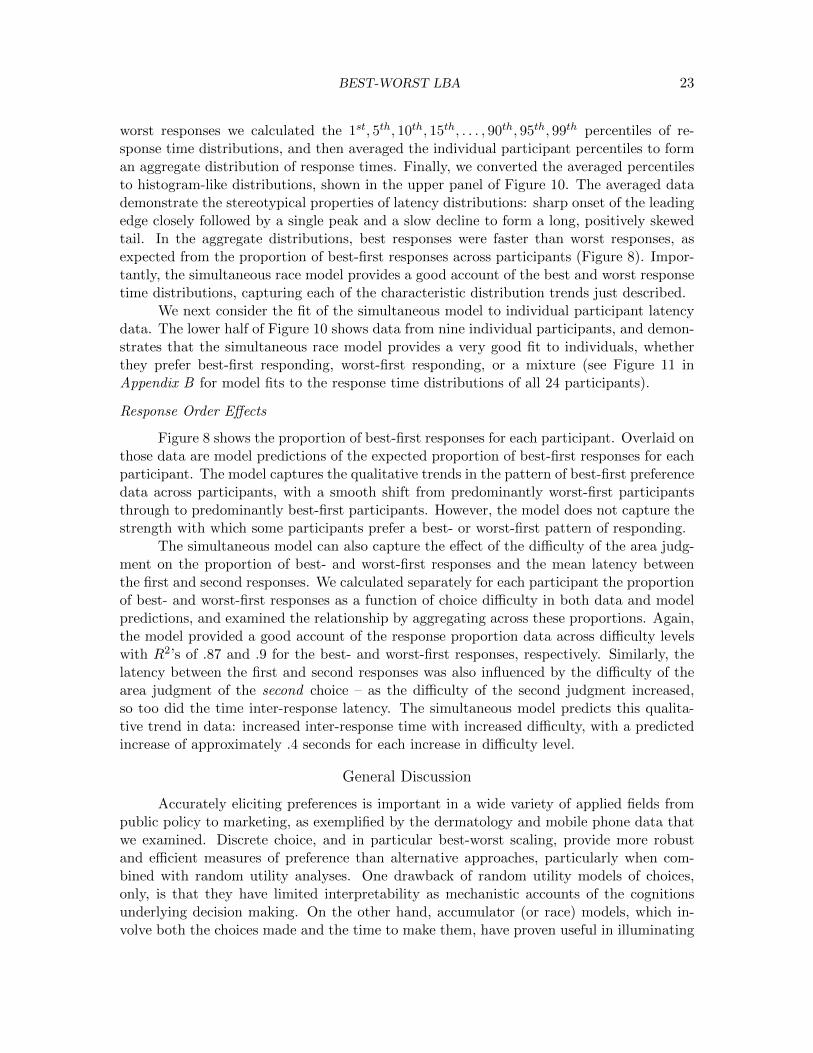
worst responses we calculated the 1st, 5th, 10th, 15th, . . . , 90th, 95th, 99th percentiles of re-sponse time distributions, and then averaged the individual participant percentiles to forman aggregate distribution of response times. Finally, we converted the averaged percentilesto histogram-like distributions, shown in the upper panel of Figure 10. The averaged datademonstrate the stereotypical properties of latency distributions: sharp onset of the leadingedge closely followed by a single peak and a slow decline to form a long, positively skewedtail. In the aggregate distributions, best responses were faster than worst responses, asexpected from the proportion of best-first responses across participants (Figure 8). Impor-tantly, the simultaneous race model provides a good account of the best and worst responsetime distributions, capturing each of the characteristic distribution trends just described.
We next consider the fit of the simultaneous model to individual participant latencydata. The lower half of Figure 10 shows data from nine individual participants, and demon-strates that the simultaneous race model provides a very good fit to individuals, whetherthey prefer best-first responding, worst-first responding, or a mixture (see Figure 11 inAppendix B for model fits to the response time distributions of all 24 participants).
Response Order Effects
Figure 8 shows the proportion of best-first responses for each participant. Overlaid onthose data are model predictions of the expected proportion of best-first responses for eachparticipant. The model captures the qualitative trends in the pattern of best-first preferencedata across participants, with a smooth shift from predominantly worst-first participantsthrough to predominantly best-first participants. However, the model does not capture thestrength with which some participants prefer a best- or worst-first pattern of responding.
The simultaneous model can also capture the effect of the difficulty of the area judg-ment on the proportion of best- and worst-first responses and the mean latency betweenthe first and second responses. We calculated separately for each participant the proportionof best- and worst-first responses as a function of choice difficulty in both data and modelpredictions, and examined the relationship by aggregating across these proportions. Again,the model provided a good account of the response proportion data across difficulty levelswith R2’s of .87 and .9 for the best- and worst-first responses, respectively. Similarly, thelatency between the first and second responses was also influenced by the difficulty of thearea judgment of the second choice – as the difficulty of the second judgment increased,so too did the time inter-response latency. The simultaneous model predicts this qualita-tive trend in data: increased inter-response time with increased difficulty, with a predictedincrease of approximately .4 seconds for each increase in difficulty level.
General Discussion
Accurately eliciting preferences is important in a wide variety of applied fields frompublic policy to marketing, as exemplified by the dermatology and mobile phone data thatwe examined. Discrete choice, and in particular best-worst scaling, provide more robustand efficient measures of preference than alternative approaches, particularly when com-bined with random utility analyses. One drawback of random utility models of choices,only, is that they have limited interpretability as mechanistic accounts of the cognitionsunderlying decision making. On the other hand, accumulator (or race) models, which in-volve both the choices made and the time to make them, have proven useful in illuminating

BEST-WORST LBA 24
the cognitive and neurophysiological processes underpinning simple single-attribute deci-sions. Over the last several decades there have been increasingly successful and practicalapplications of accumulator models to multi-attribute preference data, including decisionfield theory (Busemeyer & Townsend, 1992, 1993; Roe et al., 2001), the leaky competingaccumulator model (Usher & McClelland, 2004), the Poisson race model (Otter et al., 2008;Ruan et al., 2008), and most recently the 2N -ary choice model (Wollschlager & Diederich,2012). Our proposal builds on these developments and applies them to a more complexchoice task, best-worst scaling, with the aim of producing a model that has both tractablestatistical properties and a plausible cognitive interpretation. This is an example of “cog-nitive psychometrics”, which aims to combine psychological insights from process-basedmodeling with the statistical advantages of measurement approaches (see, e.g., Batchelder,2009; van der Maas, Molenaar, Maris, Kievit, & Borsboom, 2011).
In the first section of this paper we demonstrated how a simplified accumulator model(LBA: Brown & Heathcote, 2008) can make race models practical for the analysis of thecomplex, multi-attribute best-worst decisions typically required in many applications. Thethree MNL-inspired LBA variants we examined were all capable of fitting choice data atleast as well as the best random utility models of choice. The parameter estimates fromthe race models were closely related to the parameter estimates from the random utilitymodels, providing further confidence in the use of the race models to describe data.
In the second section of this paper we demonstrated the benefit that response timesadd to understanding the cognitive processes underpinning best-worst choice. In the contextof a best-worst response procedure implemented in a simple perceptual experiment, weprovided evidence against the assumptions of the three LBA models proposed in the firstsection, and by extension provided evidence against some assumptions of the MNL modelsfrom which they were derived. We then modified one of the LBA models to develop a newsimultaneous best race and worst race model. The simultaneous model provided a goodaccount of data at the individual participant and aggregate levels, for both choices andresponse times, including a range of newly identified phenomena relating to the effect ofdecision difficulty on the order and speed of best and worst responses.
Further work remains to determine whether the simultaneous model can account forthe longer scale response times produced by complex multi-alternative choices, and whethera single model can accommodate best-only and best-worst choices with these types of stim-uli. For both simple and complex choices there are challenges remaining related to thefine-grained measurement and modeling of the time to make both best and worst choices.Methodologically it would be desirable to use a faster response method than moving apointer with a mouse and clicking a target to minimize the motor component of inter-response time. Recent approaches using eye movements appear promising in this regard(Franco-Watkins & Johnson, 2011a, 2011b). A complimentary approach would be to elab-orate the simultaneous model to accommodate the time course of motor processes and toaddress paradigms like ours that by design do not allow the same best and worst response.
The main advantage of the LBA approach over earlier process models is its mathe-matical tractability. However, a disadvantage when compared with more complete models,such as decision field theory and the leaky competing accumulator model, is that the LBAmodels we have developed do not describe various context effects that occur in preferentialchoice. This happens because the LBA models belong to the class of “horse race” ran-

BEST-WORST LBA 25
dom utility models (Marley & Colonius, 1992), which are known to fail at explaining manycontext effects (see Rieskamp, Busemeyer, & Mellers, 2006). However, Trueblood, Brown,Heathcote, and Busemeyer (in preparation) have recently extended the LBA approach toinclude contexts effects in a way that retains its computational advantages.
We conclude by proposing that – even though further development is desirable – thesimultaneous race model as it stands is a viable candidate to replace traditional randomutility analysis of data obtained by best-worst scaling. The simultaneous model providesan account of choice data equivalent to the MNL choice models, but in addition it accountsfor various patterns in response time data and provides a plausible explanation of the latentdecision processes involved in best-worst choice.
Acknowledgments
This research has been supported by Natural Science and Engineering Research Coun-cil Discovery Grant 8124-98 to the University of Victoria for Marley. The funding sourcehad no role in study design, or in the collection, analysis and interpretation of data. Thework was carried out, in part, whilst Marley was a Distinguished Professor in the Centrefor the Study of Choice, University of Technology, Sydney.

BEST-WORST LBA 26
Appendix A: The Maxdiff Model for Best-Worst Choice
Using the generic notation of Figure 2, BWX(x, y) is the probability of choosing xas best and y 6= x as worst when the available set of options is X. The maxdiff model forbest-worst choice assumes that the utility of a choice option in the selection of a best option(u) is the negative of the utility of that option in the selection of a worst option (−u) andthat
BWX(x, y) =e[u(x)−u(y)]∑
{p,q}∈Xp 6=q
e[u(p)−u(q)](x 6= y). (1)
For the Flynn et al. (2008) data and analyses, X is a set of attribute levels, and so xand y are the attribute levels selected as best and worst, respectively. Marley et al. (2008)present mathematical conditions under which all the attribute levels are measured on acommon difference scale; in this case, the utility of one attribute level can be set to zero.
For the Marley and Pihlens (2012) best-worst data and analyses, X is a set of multi-attribute profiles, and so x and y are the profiles selected as best and worst, respectively.Marley and Pihlens also assume that each profile has an additive representation over theattribute levels; that is, assuming that each profile has m attributes, then there are utilityscales ui, i = 1, ...m, such that if z = (z1, ...zm), with zi the attribute level for z on attributei, then
u(z) =m∑
i=1
ui(zi).
Marley and Pihlens (2012) present a set of mathematical conditions under which the utilityof a profile is such a sum of the utilities of its attribute levels, and each attribute is measuredon a separate difference scale; in this case, one level on each attribute can have its utilityset to zero.
BEST-WORST LBA 27
Appendix B: Simultaneous LBA Model Fits to IndividualParticipant Response Time Distributions
In this Appendix we show the fit of the simultaneous race model to response timedistributions at the level of individual participant data, for all 24 participants. Each panelof Figure 11 shows the fit of the race model to a separate participant. As described in themain text, there are clear individual differences in the pattern of responding – best-first,worst-first, or no preference for either best- or worst-first – as well as the time course ofdecisions – some participants made much faster responses than others. For both patternsof individual differences the simultaneous model provides a good account of the latencydistributions from the majority of participants.

BEST-WORST LBA 28
References
Batchelder, W. H. (2009). Cognitive psychometrics: Using multinomial processing tree models asmeasurement tools. In S. E. Embretson (Ed.), Measuring psychological constructs: Advancesin model based measurement. American Psychological Association Books.
Brown, S., & Heathcote, A. J. (2008). The simplest complete model of choice reaction time: Linearballistic accumulation. Cognitive Psychology, 57, 153–178.
Brown, S., Marley, A. A. J., Donkin, C., & Heathcote, A. (2008). An integrated model of choicesand response times in absolute identification. Psychological Review, 115, 396–425.
Busemeyer, J. R., & Townsend, J. T. (1992). Fundamental derivations from decision field theory.Mathematical Social Sciences, 23, 255–282.
Busemeyer, J. R., & Townsend, J. T. (1993). Decision field theory: A dynamic–cognitive approachto decision making. Psychological Review, 100, 432–459.
Coast, J., Salisbury, C., de Berker, D., Noble, A., Horrocks, S., Peters, T. J., & Flynn, T. N. (2006).Preferences for aspects of a dermatology consultation. British Journal of Dermatology, 155,387–392.
Collins, A. T., & Rose, J. M. (2011). Estimation of stochastic scale with best–worst data. Manuscript,University of Sydney.
Dellaert, B. G. C., Donkers, B., & van Soest, A. (2012). Complexity effects in choice experiment-based models. Journal of Marketing Research, 49, 424–434.
Diederich, A., & Busemeyer, J. R. (2003). Simple matrix methods for analyzing diffusion modelsof choice probability, choice response time, and simple response time. Journal of MathematicalPsychology, 47, 304–322.
Finn, A., & Louviere, J. J. (1992). Determining the appropriate response to evidence of publicconcern: The case of food safety. Journal of Public Policy and Marketing, 11, 12–25.
Flynn, T. N., Louviere, J. J., Peters, T. J., & Coast, J. (2007). Best–worst scaling: What it can dofor health care research and how to do it. Journal of Health Economics, 26, 171–189.
Flynn, T. N., Louviere, J. J., Peters, T. J., & Coast, J. (2008). Estimating preferences for adermatology consultation using best–worst scaling: Comparison of various methods of analysis.BMC Medical Research Methodology, 8 (76).
Flynn, T. N., Louviere, J. J., Peters, T. J., & Coast, J. (2010). Using discrete choice experimentsto understand preferences for quality of life. Social Science & Medicine, 70, 1957–1965.
Flynn, T. N., & Marley, A. A. J. (submitted). Best-worst scaling: Theory and methods. In S. Hess& A. Daly (Eds.), Handbook of Choice Modelling.
Forstmann, B. U., Dutilh, G., Brown, S., Neumann, J., von Cramon, D. Y., Ridderinkhof, K. R.,& Wagenmakers, E.-J. (2008). The striatum facilitates decision–making under time pressure.Proceedings of the National Academy of Science, 105, 17538–17542.
Franco-Watkins, A. M., & Johnson, J. G. (2011a). Applying the decision moving window torisky choice: Comparison of eye–tracking and mouse–tracing methods. Judgment and DecisionMaking, 6, 740–749.
Franco-Watkins, A. M., & Johnson, J. G. (2011b). Decision moving window: Using interactive eyetracking to examine decision processes. Behavior Research Methods, 43, 853–863.

BEST-WORST LBA 29
Frank, M. J., Scheres, A., & Sherman, S. J. (2007). Understanding decision making deficits in neuro-logical conditions: Insights from models of natural action selection. Philosophical Transactionsof the Royal Society, Series B, 362, 1641–1654.
Gilchrist, W. (2000). Statistical modelling with quantile functions. London: Chapman & Hall/CRC.
Goodman, S. N. (2009). An international comparison of retail wine consumer choice. InternationalJournal of Wine Business Research, 21, 41–49.
Haaijer, R., Kamakura, W., & Wedel, M. (2000). Response latencies in the analysis of conjointchoice experiments. Journal of Marketing Research, 37, 376–382.
Heathcote, A., & Love, J. (2012). Linear deterministic accumulator models of simple choice. Frontiersin Psychology, 3, n/a. doi: 10.3389/fpsyg.2012.00292.
Ho, T., Brown, S., & Serences, J. (2009). Domain general mechanisms of perceptual decision makingin human cortex. Journal of Neuroscience, 29, 8675–8687.
Lee, J. A., Soutar, G. N., & Louviere, J. J. (2008). The best–worst scaling approach: An alternativeto Schwartz’s values survey. Journal of Personality Assessment, 90, 335–347.
Louviere, J. J., & Flynn, T. N. (2010). Using best–worst scaling choice experiments to measure publicperceptions and preferences for healthcare reform in Australia. The Patient: Patient–CenteredOutcomes Research, 3, 275–283.
Louviere, J. J., & Islam, T. (2008). A comparison of importance weights and willingness-to-pay measures derived from choice–based conjoint, constant sum scales and best–worst scaling.Journal of Business Research, 61, 903–911.
Luce, R. D. (1959). Individual choice behavior: A theoretical analysis. New York: Wiley.
Luce, R. D. (1986). Response times. New York: Oxford University Press.
Marley, A. A. J. (1989). A random utility family that includes many of the “classical” models andhas closed form choice probabilities and choice reaction times. British Journal of Mathematicaland Statistical Psychology, 42, 13–36.
Marley, A. A. J., & Colonius, H. (1992). The “horse race” random utility model for choice prob-abilities and reaction times, and its competing risks interpretation. Journal of MathematicalPsychology, 36, 1–20.
Marley, A. A. J., Flynn, T. N., & Louviere, J. J. (2008). Probabilistic models of set-dependent andattribute-level best-worst choice. Journal of Mathematical Psychology, 52, 281–296.
Marley, A. A. J., & Islam, T. (2012). Conceptual relations between expanded rank data and modelsof the unexpanded rank data. Journal of Choice Modelling, 5, 38–80.
Marley, A. A. J., & Louviere, J. J. (2005). Some probabilistic models of best, worst, and best–worstchoices. Journal of Mathematical Psychology, 49, 464–480.
Marley, A. A. J., & Pihlens, D. (2012). Models of best–worst choice and ranking among multiat-tribute options (profiles). Journal of Mathematical Psychology, 56, 24–34.
Mueller, S., Lockshin, L., & Louviere, J. J. (2010). What you see may not be what you get: Askingconsumers what matters may not reflect what they choose. Marketing Letters, 21, 335–350.
Mueller Loose, S., & Lockshin, L. (2013). Testing the robustness of best worst scaling for cross-national segmentation with different numbers of choice sets. Food Quality and Preference, 27,230–242.

BEST-WORST LBA 30
Otter, T., Allenby, G. M., & van Zandt, T. (2008). An integrated model of discrete choice andresponse time. Journal of Marketing Research, 45, 593–607.
Paulhus, D. L. (1991). Measurement and control of response bias. In J. P. Robinson, P. R. Shaver, &L. S. Wrightsman (Eds.), Measures of personality and social psychological attitudes (pp. 17–59).San Diego, CA: Academic Press.
R Development Core Team. (2012). R: A language and environment for statistical computing.Vienna, Austria. (ISBN 3–900051–07–0)
Ratcliff, R. (1978). A theory of memory retrieval. Psychological Review, 85, 59–108.
Ratcliff, R., & Rouder, J. N. (1998). Modeling response times for two–choice decisions. PsychologicalScience, 9, 347–356.
Ratcliff, R., & Smith, P. L. (2004). A comparison of sequential sampling models for two–choicereaction time. Psychological Review, 111, 333–367.
Rieskamp, J., Busemeyer, J. R., & Mellers, B. A. (2006). Extending the bounds of rationality:Evidence and theories of preferential choice. Journal of Economic Literature, 44, 631–661.
Roe, R. M., Busemeyer, J. R., & Townsend, J. T. (2001). Multi–alternative decision field theory:A dynamic artificial neural network model of decision–making. Psychological Review, 108,370–392.
Ruan, S., MacEachern, S. N., Otter, T., & Dean, A. M. (2008). The dependent Poisson race modeland modeling dependence in conjoint choice experiments. Psychometrika, 73, 261–288.
Ryan, M., & Farrar, S. (2000). Using conjoint analysis to elicit preferences for health care. BritishMedical Journal, 320, 1530–1533.
Szeinbach, S. L., Barnes, J. H., McGhan, W. F., Murawski, M. M., & Corey, R. (1999). Usingconjoint analysis to evaluate health state preferences. Drug Information Journal, 33, 849–858.
Trueblood, J. S., Brown, S. D., Heathcote, A., & Busemeyer, J. R. (in preparation). The multi-attribute linear ballistic accumulator model of context effects in multi-alternative choice.
Trueblood, J. S., Brown, S. D., Heathcote, A., & Busemeyer, J. R. (in press). Not just for consumers:Context effects are fundamental to decision–making. Psychological Science.
Usher, M., & McClelland, J. L. (2004). Loss aversion and inhibition in dynamical models ofmultialternative choice. Psychological Review, 111, 757–769.
van der Maas, H. L. J., Molenaar, D., Maris, G., Kievit, R. A., & Borsboom, D. (2011). Cognitivepsychology meets psychometric theory: On the relation between process models for decisionmaking and latent variable models for individual differences. Psychological Review, 118, 339–356.
van Zandt, T., Colonius, H., & Proctor, R. W. (2000). A comparison of two response time modelsapplied to perceptual matching. Psychonomic Bulletin & Review, 7, 208–256.
Wollschlager, L. M., & Diederich, A. (2012). The 2N-ary choice tree model for N-alternativepreferential choice. Frontiers in Psychology, 3, n/a. doi: 10.3389/fpsyg.2012.00189.

BEST-WORST LBA 31
Table 2: The nine attributes and their combined 38 levels from Marley and Pihlens (2012). Thevalues in parentheses indicate the coding used in Figures 4 and 5 below.
Attribute Attribute levels
Phone style (s) Clam or flip phone (1)Candy bar or straight phone (2)Slider phone (3)Swivel phone (4)Touch screen phone (5)PDA phone with a HALF QWERTY keyboard (6)PDA phone with a FULL QWERTY keyboard (7)PDA phone with touch screen input (8)
Brand (b) A (1)B (2)C (3)D (4)
Price (p) $49.00 (1)$129.00 (2)$199.00 (3)$249.00 (4)
Camera (c) No camera (1)2 megapixel camera (2)3 megapixel camera (3)5 megapixel camera (4)
Wireless connectivity (w) No bluetooth or WiFi connectivity (1)WiFi connectivity (2)Bluetooth connectivity (3)Bluetooth and WiFi connectivity (4)
Video capability (v) No video recording (1)Video recording (up to 15 min; 2)Video recording (up to 1 h; 3)Video recording (more than 1 h; 4)
Internet capability (i) Internet access (1)No internet access (2)
Music capability (m) No music capability (1)MP3 music player only (2)FM radio only (3)MP3 music player and FM radio (4)
Handset memory (r) 64 MB built-in memory (1)512 MB built-in memory (2)2 GB built-in memory (3)4 GB built-in memory (4)

BEST-WORST LBA 32
Table 3: The nine rectangular stimuli generated by factorially crossing three rectangle widths withthree rectangle heights. All measurements are in pixels.
Width Height Area
55 110 605055 121 665555 133 731561 110 671061 121 738161 133 811367 110 737067 121 810767 133 8911

BEST-WORST LBA 33
Choices−Only
6000 7000 8000 9000
Rectangle Area (pixels)
−2
−1
0
1
2
Mean L
og D
rift R
ate
Response Times
6000 7000 8000 9000
0 .2 .4 .6 .8 1
Best C
hoic
e
Pro
babili
ties fro
m L
BA
Best Choice Proportions from Data
0
.2
.4
.6
.8
1R
2= .997
0 .2 .4 .6 .8 1
Wors
t C
hoic
e
Pro
babili
ties fro
m L
BA
Worst Choice Proportions from Data
0
.2
.4
.6
.8
1R
2= .98
0 .2 .4 .6 .8 1
R2
= .966
0 .2 .4 .6 .8 1
R2
= .953
Figure 9. Estimated drift rates and goodness of fit to data for the simultaneous race model whenfit to choices, only, and choices and response times (left and right columns, respectively). The upperpanels show mean estimated log drift rates as a function of rectangle area. Error bars indicatewithin-subjects standard errors of the mean. The middle and lower panels show the goodness offit to the experimental data for best and worst responses, respectively. The x-axes display choiceproportions from data, the y-axes display predicted choice probabilities from the simultaneous racemodel, and the diagonal lines show a perfect fit. In the lower panels, each participant contributed9 data points to each panel – one for each rectangle area.

BEST-WORST LBA 34
0 2 4 6 8 10
0
.1
.2
.3
.4
Response Time (seconds)
De
nsity
Aggregate Fit
Best − Data
Best − Model
Worst − Data
Worst − Model
1.2 4.4 7.5 10.7
Best−first
1 3.7 6.4 9.1
.7 1.7 2.6 3.6
1.1 6.3 11.6 16.8
Individual Participants
Worst−first
.9 4.7 8.4 12.2
1 3.9 6.9 9.8
Response Time (seconds)
1.2 5.9 10.5 15.2
No preference
1.2 6.1 10.9 15.8
1.4 5.8 10.1 14.5
Figure 10. Response time distributions for experimental data and predictions from the simultaneousrace model. The upper panel shows quantile averaged data as stepped histograms with best andworst responses shown in black and gray, respectively. The smooth density curves show modelpredictions with best and worst predictions shown in green and red, respectively, averaged in thesame way as the data. The lower panels display model fits to a selection of individual participantdata. We show participants broadly classified into three categories of responders: those who tendedto respond with the best option first, the reverse who tended to respond with the worst optionfirst, and those participants that demonstrated no strong preference for either best or worst firstresponding. For model fits to all 24 participants see Figure 11 in Appendix B.

BEST-WORST LBA 35
.5 3.2 6 8.7
1.2 4.4 7.5 10.7
1.2 6.1 10.9 15.8
.8 5.9 11 16.1
1 4.1 7.3 10.4
1.2 5.9 10.5 15.2
.7 4.4 8.2 11.9
Response Time (seconds)
.7 3.3 6 8.6
.9 4.7 8.4 12.2
1 3.7 6.4 9.1
1.1 4.6 8.1 11.6
1 5.7 10.4 15.1
.6 3.8 6.9 10.1
1.4 5.9 10.3 14.8
1.4 5.8 10.1 14.5
1.3 4.8 8.2 11.7
1 2.9 4.9 6.8
1.7 4.8 7.9 11
1.3 3.7 6 8.4
.9 4.4 8 11.5
1.1 6.3 11.6 16.8
.9 4.1 7.4 10.6
1 3.9 6.9 9.8
.7 1.7 2.6 3.6
Figure 11. Response time distributions for experimental data and predictions from the simultaneousrace model. Each panel shows a separate participant. Data are shown as stepped histograms withbest responses in black and worst responses in gray. Model predictions are shown as smooth densitycurves with best predictions in green and worst in red.