integrating goal programming in biomass … vol 1-no 2/integrating... · goal programming was used...
TRANSCRIPT
ABS
TRAC
TEMERGING AREA CONTRIBUTIONS
45J-FOR Journal of Science & Technology for Forest Products and Processes: VOL.1, NO.2, 2011
Goal programming was used to analyze biomass procurement value chains in the case of competing goals for power plants. One cost and six quality goals, namely moisture and ash contents and thermal values of each of two biomass types, were selected. Four model scenarios were investigated: i) benchmark total cost and upper bounds of the mean values of the six biomass properties (Initial Goals), ii) relaxing the quality goals by 10% from the Initial Goals scenario, iii) relaxing the quality goals by 20% from the Initial Goals scenario, and iv) all goals as in Initial Goals except that the Atikokan Generating Station (AGS) is supplied with only unutilized or underutilized biomass. Varying degrees of increase in total costs as well as costs for each power plant compared to the benchmark costs were observed for the other scenarios. The highest increase in total cost (7.54%) was observed for the scenario in which the AGS plant uses only unutilized or underutilized biomass.
THAKUR UPADHYAY, REINO PULKKI*, CHANDER SHAHI, MATHEW LEITCH, AND BEDARUL ALAM
INTEGRATING GOAL PROGRAMMINGIN BIOMASS PROCUREMENT FOR BIO-ENERGY VALUE CHAINS
Use of bio-energy combined with other green energy sources such as hydro, wind, and solar power can contribute to reduc-ing significantly our dependency on fos-sil fuels, thereby reducing greenhouse gas (GHG) emissions. Woody biomass is be-coming more and more important as an alternative green energy source because it is available as a sustainable renewable resource and is CO2-neutral in terms of its production and consumption for en-ergy purposes [1–3]. However, energy production from such woody biomass faces many challenges, including the un-certainty of biomass feedstock supply be-cause of its sparse availability over space
and time [1,4,5]. Furthermore, increasing demand for biomass feedstock for bioen-ergy production, as more biomass-based power plants come into operation, is caus-ing a significant increase in transporta-tion distances, leading to higher biomass procurement costs [6–8]. In this context, modelling biomass procurement cost structures under various resource con-straints, competition, and various goals/targets for a group of power plants in the Canadian boreal region is of particular importance for understanding bio-energy value chains.
With the oil crisis in the 1970s and the consequent rapid rise in oil prices, there was
much interest in Canada in biomass for bio-energy production, as demonstrated by the peak in research and development funding for the ENFOR (Energy from the Forest) program in the early 1980s [9]. However, with the ongoing decrease in oil prices from the mid-1980s until re-cently, research in biomass for bio-energy value chains was much reduced. In recent years, Canada’s degree of dependence on fossil fuels has changed, and forest bio-mass is again playing an important part in Canada’s energy consumption picture, supplying approximately 4.7% of primary energy demand and becoming the second-largest source of renewable energy after
INTRODUCTION
MATHEW LEITCH Faculty of Natural Resources ManagementLakehead UniversityThunder Bay, ONCanada
REINO PULKKIFaculty of Natural Resources ManagementLakehead UniversityThunder Bay, ONCanada
THAKUR UPADHYAY Faculty of Natural Resources ManagementLakehead UniversityThunder Bay, ONCanada
CHANDER SHAHI Faculty of Natural Resources ManagementLakehead UniversityThunder Bay, ONCanada
*Contact: [email protected]
BEDARUL ALAM Faculty of Natural Resources ManagementLakehead UniversityThunder Bay, ONCanada
46 J-FOR Journal of Science & Technology for Forest Products and Processes: VOL.1, NO.2, 2011
hydroelectricity [10]. There has also been recent pressure on developed countries through various international climate poli-cies to limit their GHG emissions. Con-sequently, the Canadian government has made a commitment to reduce GHG emissions in its major industrial sectors. In this context, the forest products indus-try of Canada has been a leader in using bioenergy (e.g., by burning black liquor and hog fuel to provide a major part of its energy needs). Beyond the forest industry, several independent power plants are gen-erating electricity from forest biomass. For example, use of wood biomass for bioen-ergy production has recently increased dramatically in northwestern Ontario (NWO), with four major energy plants.
Currently, three major combined heat and power (CHP) plant develop-ments in NWO (specifically, west of Lake Nipigon) have the potential to use forest biomass feedstock for energy production. These include Resolute Forest Products Thunder Bay CHP Plant (ABTB), Reso-lute Forest Products Fort Frances CHP Plant (ABFF), and Domtar Dryden CHP Plant (DDPP), with power generating ca-pacities of 61 MWe and 16 MWth, 50 MWe and 61 MWth, and 30 MWe and 37 MWth respectively. The Atikokan Generating Station (AGS), another power plant in NWO, is currently being converted to use forest biomass feedstock instead of coal. Its power generating capacity is 230 MWe, but the plan is to run it at 10% capacity [11,12]. The combined annual demand of approximately 2.21 million green tonnes (gt) of biomass feedstock by these four power plants is significant and will there-fore generate major socio-environmental consequences for the region. If bioenergy production is fully developed in this re-gion, it will not only help reduce green-house gas (GHG) emissions, but will also help to stabilize the economy of many small rural communities.
The biomass currently used consists mainly of mill and logging residues, but in the future, currently underutilized spe-cies and unmerchantable standing trees will need to be used to meet the growing
demands for biomass. In this study, the en-tire forest-based biomass stream is classi-fied into two sources: FHR, forest harvest residue, which includes tops, branches, and wood left after stand harvesting; and UUW, unutilized or underutilized wood, which includes currently unharvested tree spe-cies that are not commercially important for timber. There are numerous options for procuring forest biomass (terrain chip-ping/grinding, roadside chipping/grind-ing, terminal chipping/grinding, bundling, etc.) and several loading and trucking op-tions. These biomass sources have various costs and properties and various potential impacts on other wood users (e.g., using standing trees for energy would compete with other wood users). Moreover, the biomass supply-chain conditions and de-mands change continuously throughout the year. The main challenge in supplying the four power plants with 2.21 million gt of biomass annually is at present to meet the demand while also meeting multiple targets in terms of the costs and proper-ties of the feedstock.
Very few studies have been carried out on wood biomass for bioenergy sup-ply chains in Canada [13–16]. Most of the studies that exist focus on optimizing har-vesting and transportation of raw material for the forest products industries from forest management units (FMUs) to the processing facilities. However, the authors found no studies relating to optimization of forest biomass feedstock supply from the forests to power plants for energy pro-duction, taking various costs and quality goals/targets into consideration, in NWO. The NWO study area is 167,184 km2, with an annual average harvest of 60,867 ha (2002–2009), which is 0.61% of the pro-ductive forest area per year. The aim of this paper is to study how goal program-ming can be integrated into the wood bio-mass-for-bioenergy value chain in NWO given the presence of competing goals (four power plants competing for the given biomass feedstock, which has vari-able characteristics). Various sets of goals are analyzed, and the results are compared with those from a reference scenario
consisting of a cost minimization prob-lem in which other physical targets were not set, but were generated by a linear programming model (the benchmark LP model described in the Model Scenario section below). The goals or targets in the model are: minimize the procurement cost ($·gt-1) of biomass; maximize the use of harvest residues and unutilized biomass; maximize the use of high-quality biomass with higher thermal value; and minimize the moisture and ash contents of the bio-mass feedstock. The variations in quality characteristics (thermal value, moisture content, and ash content) of the biomass distributed over the productive forest cells drive the results relating to cost structures with respect to different sets of goals or targets.
METHOD AND DATA
Goal Programming Model In the past, multi-criteria decision-making (MCDM) models, which is a common name given to all relevant multi-objective decision model (MODM) techniques and other related simulation models, have been used to solve complex production and management problems in various nat-ural resource management fields, includ-ing forestry [17,18]. The goal program-ming (GP) model, a variant of MODM, has been found to be particularly useful in production systems analysis because it can handle continuous problems involv-ing the optimization of several simulta-neous objectives [3]. The first GP model was reported in [19] and was developed to address the problem of infeasibilities caused by incompatible constraints. GP is an extension of linear programming (LP), which was developed to handle multiple, usually conflicting objectives in optimiza-tion problems. LP enables a firm to set the target levels of goals for various ob-jectives in a complex decision-making en-vironment. Unlike traditional LP models that deal with only one objective function to be either maximized or minimized sub-ject to various resource constraints, GP

EMERGING AREA CONTRIBUTIONS
47J-FOR Journal of Science & Technology for Forest Products and Processes: VOL.1, NO.2, 2011
models are more relevant to analyzing the multiple objectives of an economic agent. References [20] and [21] represent a pioneering effort to criticize the tradi-tional “rational economic man” approach with its single objective function of either maximizing profit/utility or minimizing costs, in which LP models can be used to solve such single-objective optimization problems. These researchers extended the rational agent model with its single objec-tive function to multiple objectives with a “satisficing approach” in which the agent can have multiple objectives which form a hierarchy and in which the profit maxi-mization/cost minimization issue may not arise. Problems structured using the sat-isficing approach are well handled by GP models. The general specification of a typical GP model is:Minimize Z = P + N (1)Subject toAX - P + N = G (2)BX ≤ R (3)P*N = 0 (4)X≥ 0 where P and N are vectors of positive de-viations (overachievement of the target or goal) and negative deviations (under-achievement of the target or goal); A and B are matrices of technical coefficients relating to goal target levels and resource constraints respectively; R and G are vec-tors of resource stock/system require-ments and targets/goals respectively; X is a vector of decision variables in the model with non-negativity constraints; and Z is a scalar sum of P and N.
In this GP specification, there are no Xs in the objective function (Eq. 1), and the objective functions are brought into the constraints with embedded posi-tive and negative deviations, as shown in Eq. (2), which is also called a set of goal constraints. Equation 3 represents the re-source and other technical constraints, and Eq. (4) restricts the model to choose either P or N for a given goal equation, but not both simultaneously. Furthermore, this standard GP model can be modified to minimize only P, only N, or both for a giv-
en objective function with certain goal(s).
Study Area and Data
The study area, 324 km×516 km (167,184 km2), consists of 18 forest management units (FMUs) and is located west of Lake Nipigon in NWO. Here, four power plants are currently operating with biomass as their feedstock. GIS data related to forest areas and depleted forest for the period from 2002 to 2009 were collected from Land Information Ontario Sustainable Forest Licence (SFL) holders and consult-ing firms in Shapefile and Geodatabase formats. The original vector data were first converted to raster format and finally to spatial database text files for the entire re-search area using ArcGIS software. Three main spatial layers (land use, forest deple-tion, and a cost layer) were prepared on a raster grid size of 1 km×1 km (1 km2). This study examines 19,315 productive forest cells where timber harvesting activi-ties occurred between 2002 and 2009 (for-est depletion cells). The detailed method-ology for estimating forest harvest residue and unutilized or underutilized biomass
availability for all 19,315 forest deple-tion cells has been described in Alam et al. (2011). To estimate per-gt transport costs from each of the forest cells to each power plant, a road network layer was overlaid onto the forest maps, and the least-cost network was determined using a road network optimization algorithm as described in [22]. A fixed time for loading and unloading and a delay of 2.5 hours per trip are assumed to add CAD 4.85/gt to the variable hauling cost. Thermal values, moisture content (MC), and ash content for each type of wood biomass for each forest cell were estimated based on the re-sults of studies reported in [23] and [24]. Other estimated techno-economic param-eters used in the GP model are given in Table 1.
Descriptive statistics for the biomass properties were computed for all 19,315 forest depletion cells (Table 2). This step helped to determine initial target levels for each of the quality goals. Six quality-related goals were selected, namely the moisture and ash contents of both forest biomass types (four goals) and the thermal value of each forest biomass type (two goals).
TABLE 1 Estimated parameters used in the model.
Harvesting and processing costs (FHR)
RemarksEstimateUnits
Note: CAD = Canadian dollars, BM = biomass, gt = green tonnes, y = year*Percentage of the total amount of biomass that can be extracted from the given area.**1km×1km harvesting sites in the forest area.
Harvesting and processing costs (UUW)Fixed cost due to loading/unloading overhead
CAD/gt
Description
Biomass demand of ABTB power plant Biomass demand of ABFF power plantBiomass demand of DDPP power plant
Harvesting factor*
Biomass demand of AGS power plant
Number of forest depletion cells **
CAD/gt
CAD/gt
gt/y
gt/y
gt/y
gt/y
% of BM
No
730,000
26
31
4.85
800,000
480,000
200,000
67
19,315
Power plant data
Power plant data
Power plant data
Power plant data
Authors’ estimate
[11]
[11]
[2]
[22]

2348 J-FOR Journal of Science & Technology for Forest Products and Processes: VOL.1, NO.2, 2011
These goals provided a fairly good sum-mary of biomass quality information to feed into the GP model. To estimate the values of all these parameters for the 19,315 forest depletion cells would be a daunting task, but estimated values of these variables at the FMU level give workable information.
GP Model for Biomass Procurement
The GP model is specified as minimizing the sum of positive and negative devia-
tions from the target levels as appropriate, depending on the problem being studied. The model proposed here minimizes the positive deviations of cost and heat values of FHR and UUW for each forest deple-tion cell and negative deviations of mois-ture and ash contents of the two types of biomass, FHR and UUW. The formal GP model is specified as follows:
where p1, p2j, and p3j represent the posi-tive deviation of the total cost target (C) and the thermal value target of FHR (g5)
and UUW (g6) for each forest depletion cell j; n1j, n2j, n3j, and n4j are negative deviations from target/goal levels of the moisture contents of FHR (g1) and UUW (g2) and the ash contents of FHR (g3) and UUW (g4) for each forest depletion cell j;PR is the processing (harvesting and grinding/chipping) cost ($·gt-1) of FHR at roadside; PU is the processing (harvesting and grinding/chipping) cost ($·gt-1) of UUW at roadside; DBi is the annual forest biomass demand (gt) of power plant i; ABRj is the annual technical availability (gt) of FHR in forest depletion cell j;ABUj is the annual technical availability (gt) of UUW in forest depletion cell j;TCij is the biomass transportation cost ($·gt-1) from the jth forest depletion cell to the ith power plant, including loading and unloading overhead; XBRij is the amount of annual FHR har-vested (gt) from the jth forest depletion cell for the ith power plant; XBUij is the amount of annual UUW har-vested (gt) from the jth forest depletion cell for the ith power plant; andXTBi is the annual forest biomass (gt) brought into the ith power plant.
In this GP model specification, Eqs. (6–12) are the goal constraint equations, in which the scalars on the right-hand side are the chosen goal or target, each represent-ing the decision-maker’s objectives which
TABLE 2 Descriptive statistics of biomass quality variables and target levels by scenario (n=19,315).
MinimumMean 22.62
Note: FHR = Forest Harvest Residue, UUW = Unutilized or underutilized wood biomass, gw= green weight.
Moisture Content FHR (% gw basis)
Thermal Value FHR (GJ/ODt)
Ash Content FHR (%)
Moisture Content UUW (% gw basis)
Thermal Value UUW
(GJ/ODt)
Ash Content UUW (%)
MaximumStandard deviationInitial goals10% relaxation20% relaxationUUWAGS No FHR for AGS only, but the other plants are using it.
18.92 1.59 29.77 16.99 1.87
23 19 2 30 17 2
30 17 2
27.6 22.8 2.4 36 20.4 2.425.3 20.9 2.2 33 18.7 2.2
1.51 0.47 0.56 7.21 1.29 0.45
21.60 18.50 1.30 22.50 15.30 1.0027.00 20.00 3.00 41.30 18.50 2.50
EMERGING AREA CONTRIBUTIONS
49J-FOR Journal of Science & Technology for Forest Products and Processes: VOL.1, NO.2, 2011
must be achieved through relevant devia-tions by selecting optimal values for the decision variables XBRij and XBUij. The cost target is determined based on the to-tal cost obtained from the LP model with-out goal constraints with the same techni-cal constraints as for the benchmark case. Different quality targets are selected based on the four goal-set scenarios described earlier. The Initial Goals scenario selects upper bounds for the mean values of each of the six biomass quality characteristics, as shown in Table 2. The constraints ex-pressed in Eqs. (14) and (15) represent harvesting constraints and indicate that the annual harvest for each type of bio-mass should not exceed the available bio-mass in each forest depletion cell. Equa-tion (16) requires that the total amount of forest biomass harvested for the ith power plant should at least meet the demand of that plant. The complexity of this GP formulation can be seen in Eqs. (6–12), where the tar-gets on the right-hand side are to be mul-tiplied by the decision variables for each equation to cancel out the decision vari-ables on the left-hand side so that resource characteristics described on the left-hand side become comparable with the goals (g1 – g6) on the right-hand side. This type of formulation is possible in the general algebraic modelling system (GAMS) pro-gramming language, and GAMS’s solver treats such a problem as a non-linear model. The solution procedure for the GP model selects the optimal forest deple-tion cells to harvest for FHR and UUW biomass to meet the annual feedstock requirements of each power plant while satisfying various cost and quality goals as discussed above. The moisture and ash contents of each type of biomass in forest depletion cell j can be underachieved be-cause lower values of these properties are preferred, whereas the thermal values of each type of biomass in forest depletion cell j can be overachieved because a higher thermal value is preferred to a lower one. The hierarchical goal constraints of these biomass qualities will definitely increase total procurement costs, and therefore a
positive deviation is allowed in the model.
Model Scenario
To test the various multiple-objective bio-mass procurement decision scenarios for the four power plants, four different goal-set scenarios were investigated. Before running the GP models, the benchmark LP model was run with a total cost mini-mization objective (sum of the costs for all four plants) with the usual constraints and without any quality targets (no target values set for moisture contents, thermal values, or ash contents). The results of the benchmark LP model gave an idea of cost goals and results as a basis for comparison of the biomass procurement costs for dif-ferent scenarios in the GP model. Once the GP model as specified above starts to function consistently for these selected goal-set scenarios, it can then be used to run any combination of relevant goal sets, depending on the procurement managers’ criteria for goals and objectives.
The first scenario, Initial Goals, consists of a goal set in which the bio-mass properties (MC, ash contents, and thermal values) have upper bounds equal to the mean values of the corresponding variables (Table 2). This scenario is de-fined to establish baseline goals relating to biomass quality, where the power-plant manager may want to have higher-quality feedstock as defined by these threshold goals and targets. This goal set will intro-duce constraints into the model because the biomass to be harvested should have MC and ash contents not greater than the targets and the thermal value should be at least equal to the target. The second (10% Relaxation) and third (20% Relaxation) scenarios have goal sets that relax the tar-get values for biomass properties (the tar-get values are as shown in Table 2) from the Initial Goals scenario by 10% and 20% respectively. These two scenarios were run to test the sensitivity of the changes in goal levels (targets) to the cost structures of bio-mass procurement problems. The fourth scenario involved using only unutilized or underutilized biomass for the AGS power
plant (the UUWAGS scenario) because this plant is planning to use UUW to produce pellets for power production in the future. Due to the strict ash-content requirements (<1% ash) of these high-quality pellets, only unutilized or underuti-lized biomass can be used for this purpose because logging residues would result in excessive bark and therefore too-high ash content. In this scenario, the other qual-ity goals remain the same as in the Initial Goals scenario.
RESULTS AND DISCUSSION
The results of the benchmark LP model provide an optimal solution for supply-ing forest biomass feedstock from for-est depletion cells in the case study area (19,315 forest depletion cells in the model with parameter values as shown in Table 1) to the four power plants by minimiz-ing the total annual harvesting, processing, and transportation costs of biomass sub-ject to the availability of forest biomass in each depleted forest cell, while meeting the biomass demand of each power plant. The Dryden CHP plant is located near the middle of the research area, and there are many forest cells closer to this power plant than to others, along with a denser net-work of higher-class and straighter roads; all these factors imply a lower per-gt pro-curement cost for the Dryden plant (Fig. 1). Similarly, the AbitibiBowater Thunder Bay CHP plant is located in the south-eastern part of the research area, with no competing power plant on its northern, eastern, and southern sides in the research area. The other two power plants (ABFF and AGS), which are located close to each other in the research area, must compete more strongly for forest biomass. Figure 1 shows the network of forest cells selected to harvest FHR and UUW biomass for the four power plants in the benchmark sce-nario. The model selects 11,790 and 2,991 forest depletion cells for supplying FHR and UUW respectively. The number of cells selected for FHR is greater because of its lower per-gt procurement cost com-pared to UUW (FHR is full-tree logging
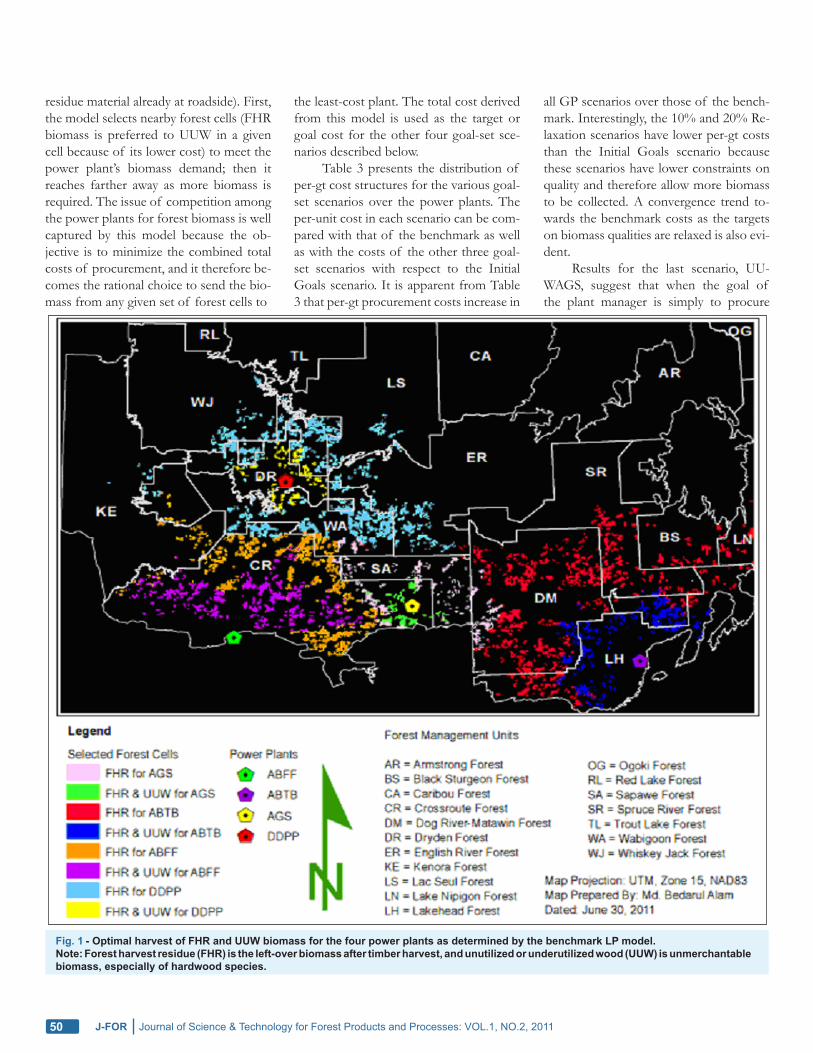
2350 J-FOR Journal of Science & Technology for Forest Products and Processes: VOL.1, NO.2, 2011
residue material already at roadside). First, the model selects nearby forest cells (FHR biomass is preferred to UUW in a given cell because of its lower cost) to meet the power plant’s biomass demand; then it reaches farther away as more biomass is required. The issue of competition among the power plants for forest biomass is well captured by this model because the ob-jective is to minimize the combined total costs of procurement, and it therefore be-comes the rational choice to send the bio-mass from any given set of forest cells to
the least-cost plant. The total cost derived from this model is used as the target or goal cost for the other four goal-set sce-narios described below.
Table 3 presents the distribution of per-gt cost structures for the various goal-set scenarios over the power plants. The per-unit cost in each scenario can be com-pared with that of the benchmark as well as with the costs of the other three goal-set scenarios with respect to the Initial Goals scenario. It is apparent from Table 3 that per-gt procurement costs increase in
all GP scenarios over those of the bench-mark. Interestingly, the 10% and 20% Re-laxation scenarios have lower per-gt costs than the Initial Goals scenario because these scenarios have lower constraints on quality and therefore allow more biomass to be collected. A convergence trend to-wards the benchmark costs as the targets on biomass qualities are relaxed is also evi-dent.
Results for the last scenario, UU-WAGS, suggest that when the goal of the plant manager is simply to procure
Fig. 1 - Optimal harvest of FHR and UUW biomass for the four power plants as determined by the benchmark LP model.Note: Forest harvest residue (FHR) is the left-over biomass after timber harvest, and unutilized or underutilized wood (UUW) is unmerchantable biomass, especially of hardwood species.

EMERGING AREA CONTRIBUTIONS
51J-FOR Journal of Science & Technology for Forest Products and Processes: VOL.1, NO.2, 2011
hardwood biomass for better-quality pellet production, the Atikokan plant has to pay more per gt, and at the same time other competing plants can grab the low-cost FHR biomass previously used by AGS, thereby reducing their unit procurement costs (compare the costs with those of the Initial Goals scenario in Table 3). These results are interesting and useful for pow-er-plant managers who wish to judge the effect of trade-offs between quality and costs, as well as the cost impacts of the strategies of other competing plants. In addition to the four goal-set scenarios, a fifth goal-set scenario was also tried in the GP model, but the model solution was in-feasible. The goal set in this scenario was to procure only FHR for all power plants under the quality goals from the Initial Goals scenario; this restriction caused the total availability of FHR biomass to be less than the total demand of the power plants. These GP model scenarios produce different distributions of optimal forest depletion cells for harvesting both types of biomass for each power plant (simi-lar to that shown in Fig. 1), and the op-timal distribution structure of forest cells changes in each scenario. Here, only the cost estimates for the model scenarios are presented in this discussion because the information required to determine a set of optimal forest cells for each scenario and each power plant is so huge that space does not permit a discussion. A database has been created containing the optimal set of forest depletion cells (from forest cell j to plant i) for each run of the model scenario. The changes in the optimal com-bination of forest depletion cells, which have logical implications for increasing or decreasing the total or unit costs of bio-mass procurement for each power plant and each model scenario, are well reflected in the cost information discussed below.
Table 4 contains the relative chang-es (in percentage terms) in total biomass procurement costs for each power plant under each model scenario. Here again, relative changes in costs can be com-pared to the benchmark and to the oth-er GP model scenarios as well as to the
Initial Goals scenario with respect to the other GP model scenarios (see the two sec-tions of Table 4). The Initial Goals scenar-io is a base scenario for the GP model, and the other scenarios in this model are based on varying the parameter values from the base case, i.e., the Initial Goals scenario. This is why it is relevant to compare the results of the three GP scenarios with the Initial Goals scenario. The highest increase in cost compared to the benchmark cost from the Initial Goals setting was seen in the ABTB plant, followed by AGS, ABFF, and DDPP in descending order.
The reasons for these variations basi-cally involve the interplay of two factors: location of the power plants in relation to biomass availability in the nearby forest cells, and the size of their demand. The AGS plant has the lowest demand, but still faces the second-highest increase in cost due to the lower availability of high-quality biomass in its vicinity and the issue of competition with the ABFF plant. The results of the scenarios involving 10% Re-laxation and 20% Relaxation in biomass properties show a smaller increase in costs for each plant, and with 20% Relaxation, the direction of change converges towards the benchmark costs. This occurs because as the quality constraints are relaxed, more biomass becomes available, and
the problem tends to mimic the GP solu-tion; this phenomenon also validates the model results. The UUWAGS scenario produced the highest increase in cost for the AGS plant (11.17%, see the fifth column of Table 4) because of the goal of harvesting only UUW biomass, which entails higher processing costs. The inter-plant externality of this goal can be seen in the slight reduction of cost for the other plants compared to the Initial Goals sce-nario (eighth column of Table 4).
The second part of Table 4 (starting from the sixth column) shows the relative changes in costs with respect to the Ini-tial Goals scenario (the base scenario of the GP model). The results of the 10% Relaxation and 20% Relaxation scenarios in this case show significant reductions in costs compared to the Initial Goals sce-nario. Only the AGS power plant under the UUWAGS scenario shows an increase of 3.69% in cost from the base scenario of the GP model; the reason for this has already been explained above.
The results in Table 4 for relative changes in costs can be summarized in terms of the impacts of the goal-set scenarios and the distribution effect of each particular scenario in terms of cost structures among the power plants. One can also observe the impacts of goal-set
TABLE 3 Biomass procurement costs in each scenario for each power plant (CAD/gt)
Power plant
SAMALA
Benchmark Initial Goals 10% Relaxation
20% Relaxation UUWAGS
ABTB
ABFF
AGS
DDPP
38.11 41.84 39.24 38.29
40.04 39.24
36.78 36.19
36.70 36.27
38.77 41.25
35.74 38.32
36.13 38.15
41.82
41.04
39.73
38.13
TABLE 4 Percentage changes in procurement costs for different scenarios for each power plant
Power plant
Initial Goals 10% Relaxation
20% Relaxation UUWAGS
ABTB
ABFF
AGS
DDPP
9.77%
10% Relaxation
20% Relaxation UUWAGS
Percentage change from benchmark costsPercentage change from Initial Goals cost scenario
6.41%
7.22%
5.60%
2.95%
3.28%
2.91%
1.56%
0.46%
1.21%
1.27%
0.37%
9.73%
5.87%
11.17%
5.53%
-6.21%
-2.94%
-4.02%
-3.82%
-8.48%
-4.89%
-5.55%
-4.95%
-0.04%
-0.51%
3.69%
-0.06%

2352 J-FOR Journal of Science & Technology for Forest Products and Processes: VOL.1, NO.2, 2011
scenarios on the total costs of biomass procurement under each scenario, as de-picted in Fig. 2. The highest total cost is associated with the UUWAGS scenario because of the use of only high-cost UUW biomass by the AGS plant, which impacted the total cost as well. The posi-tive deviations from the benchmark cost due to the introduction of goal sets in each scenario are plotted in Fig. 2 and show the difference between actual total cost and the benchmark total cost for each scenario. The lowest total cost and hence the lowest deviation from the benchmark total cost is associated with the 20% Re-laxation scenario because of the greater relaxation of biomass quality goals relative to the base scenario. The relative increases in total costs compared to the benchmark case are 7.43%, 2.78%, 0.79%, and 7.54% respectively for the Initial Goals, 10% Re-laxation, 20% Relaxation, and UUWAGS scenarios. However, the relative changes in cost for individual power plants compared to the benchmark costs vary over different scenarios from these total changes; this variation results from distributional ef-fects which can be explained by resource availability and competition factors.
Due to the introduction of quality goals in the model, the total cost has in-creased from the cost obtained from the benchmark LP model. The quality goals/ targets introduce constraints into the
model and hence increase costs relative to the LP model because the total biomass requirement and operating efficiency for each power plant remain unchanged for all the GP scenarios while quality demands increase. Furthermore, this GP model can be extended to account for the impacts of higher-quality biomass goals on procure-ment and operating cost structures as engineering equations for conversion ef-ficiency in relation to biomass quality are developed. In general, an improvement in efficiency for CHP and power-only plants would be expected with the use of higher-quality biomass (as discussed in this study), and therefore reduced total wood biomass costs in the value chain for a given amount of energy would also be expected, even though the delivery cost may be higher because of the goals requiring higher bio-mass quality. This trade-off between qual-ity and costs can be modelled. The total biomass demand for each power plant be-comes endogenous once the engineering process equations for biomass quality ver-sus conversion efficiency for each type of power plant have been introduced into the model. Development of these equations is a topic for future work.
SUMMARY AND CONCLUSIONS
Biomass procurement problems for four bio-energy power plants in NWO that
require approximately 2.21 million green tonnes (gt) of biomass annually have been analyzed using GP models. The biomass currently used is mainly mill and logging residues, but in the future, underutilized species and unmerchantable standing trees will need to be used to meet the growing demands for biomass. All biomass sources have variable costs, qualities, and poten-tial impact on other wood users (e.g., us-ing standing trees for energy would com-pete with other wood users). Moreover, the conditions and requirements in the biomass supply chain change continu-ously throughout the year. The multiple goals selected to address this problem are procurement cost plus several biomass quality properties. Six quality goals were selected: moisture and ash contents and thermal values for both forest biomass types. These provide a fairly good sum-mary of biomass quality information to feed into the GP model. After the costs and the physical quality goals had been de-termined, four different scenarios were in-vestigated, Initial Goals, 10% Relaxation, 20% Relaxation, and UUWAGS, and the results were compared with a benchmark LP cost minimization model with the usu-al constraints plus goal constraints.
The results of the model scenarios were compared with the benchmark as well as with the costs of the other three goal-set scenarios with respect to the Initial Goals scenario. The impact of the goal-set scenarios on biomass procurement costs was to increase these costs, in total as well as for each power plant, to varying degrees compared to the benchmark costs. The impacts of changing goals were inter-de-pendent between plants; changing a goal in one plant affects costs at other plants. With relaxation of quality targets or goals, the solutions showed a trend to converge towards the benchmark costs. The high-est increase in total cost was found in the scenario in which the AGS plant used only unutilized or underutilized biomass. These results from the GP models could be use-ful for power-plant managers to judge the trade-offs between biomass properties and costs, as well as the impacts on costs of the strategies of other competing plants.
Fig. 2 - Total costs (in million CAD) for biomass procurement and the increased costs relative to benchmark cost for each scenario.

EMERGING AREA CONTRIBUTIONS
53J-FOR Journal of Science & Technology for Forest Products and Processes: VOL.1, NO.2, 2011
The successful development and use of GP models as described in this study con-firms that use of such a model to analyze any combination of relevant goal sets de-pending upon the procurement managers’ goal/objective criteria can prove to be a useful decision support tool. Further-more, this GP model can be extended to account for the impacts of higher-quality biomass goals on procurement cost struc-tures once the engineering equations for conversion efficiency in relation to bio-mass quality have been developed. In general, improved efficiency of CHP and power-only plants would be expected with the use of higher-quality biomass, leading to reduced costs in the value chain for to-tal wood biomass for a given amount of energy, even though the delivery cost may be higher due to the goals requiring higher biomass quality. This trade-off between quality and costs can be modelled. The to-tal biomass demand for each power plant becomes endogenous once the engineer-ing process equations for biomass quality versus conversion efficiency for each type of power plant have been introduced into the model. Development of these equa-tions is a topic for future work.
ACKNOWLEDGEMENTS
This paper is a product of the NSERC Strategic Research Network on Value Chain Optimization. Financial support from the VCO NSERC Strategic Research Network is duly acknowledged.
REFERENCESCaputo, A.C., Palumbo, M., Pelagagge, P.M., and Scacchia, F., “Economics of Biomass Energy Utilization in Combustion and Gasification Plants: Effects of Logistic Variables,” Biomass and Bioenergy, 28:35-51 (2005). Gan, J. and Smith, C.T., “Availability of Logging Residues and Potential for Electricity Production and Carbon Displacement in the USA,” Biomass and Bioenergy, 30:1011-1020 (2006). Ballarin, A., Vecchiato, D., Tempesta, T., Marangon, F., and Troiano, T., ”BiomassEnergy Production in Agriculture: A
1.
2.
3.
Weighted Goal Programming Analysis,” Energy Policy, 39:1123-1131 (2011).Kim J., Realff, M.J., and Lee, J.H., “Optimal Design and Global Sensitivity Analysis of Biomass Supply Chain Networks for Biofuels Under Uncertainty,” Computers and Chemical Engineering, 35:1738-1751 (2011).Shahi, C., Upadhyay, T.P., Pulkki, R., and Leitch, M., “Integrated Model for Power Generation from Biomass Gasification: A Market Readiness Analysis for Northwestern Ontario,” Forestry Chronicle, 87:48-53 (2011).Rauch, P. and Gronalt, M., “The Terminal Location Problem in the Forest Fuels Supply Network,” International Journal of Forest Engineering, 21:32-40 (2010).Upadhyay, T.P., Shahi, C., Pulki, R., Leitch, M., and Xu, C., Market Readiness for Gasification of Biomass for Power Generation. A report submitted to Ontario Centre of Excellence. Faculty of Forestry and the Forest Environment, Lakehead University, Ontario, Canada (2010).Tahvanainen, T. and Perttu, A., “Supply Chain Cost Analysis of Long-Distance Transportation of Energy Wood in Finland,” Biomass and Bioenergy, 35: 3360-3375 (2011). Hall, J.P. and Richardson, J., “ENFOR—Energy from the forest,” The Forestry Chronicle, 77:831-835 (2001).Centre for Energy, Biomass Energy in Canada. Canadian Centre for Energy Information. http://www.centreforenergy.com/AboutEnergy/Biomass/Overview.asp?page=6, (2011) [Accessed 10 August 2011]. Ontario Ministry of Energy (OME), An Assessment of the Viability of Exploiting Bio-Energy Resources Accessible to the Atikokan Generating Station in Northwestern Ontario. A consultancy report prepared by Forest BioProducts, Inc., Sault Ste. Marie, Ontario, Canada (2006).Ontario Power Generation, Inc. (OPG), Atikokan Generation Station Biomass Repowering Project. Ontario Power Generation, Inc., h t tp ://www.opg. com/power/thermal/AtikokanFactSheet1009.pdf (2010) [Accessed May 25, 2011]. Pulkki, R., “Role of Supply Chain
4.
5.
6.
7.
8.
9.
10.
11.
12.
13.
Management in the Wise Use of Wood Resources,” Southern African Journal, 191:89-95 (2001). Bradley, D., Canada Biomass-Bioenergy Report. Climate Change Solutions – IEA Bioenergy Task 40-Biotrade. Canada Country Report, http://bioenergytrade.org (2006) [Accessed 15 June 2010].Chauhan, S.S., Frayret, J.M., and LeBel, L., “Multi-Commodity Supply Network Planning in the Forest Supply Chain,” European Journal of Operational Research, 196:688–696 (2009).Sowlati, T., Forest Products and Forest Biomass Transportation and Logistics, FORAC, www.forac.ulaval.ca (2009) [Accessed 28 June 2010].Romero, C. and Rehman, T., Multiple Criteria Analysis for Agricultural Decisions, Elsevier Science (1989).Upadhyay, T.P., Solberg, B., and Sankhayan, P.L., “Use of Models to Analyse Land-Use Changes, Forest/Soil Degradation and Carbon Sequestration with Special Reference to Himalayan Region: A Review and Analysis,” Forest Policy and Economics, 9:349-371 (2006).Charnes, A. and Cooper, W.W., Management Models and Industrial Applications of Linear Programming, New York: John Wiley (1961).Simon, H.A., “A Behavioral Model of Rational Choice,” Quarterly Journal of Economics, 69:99-118 (1955).Arrow, K.J., Limited Knowledge and Economic Analysis, American Economic Review, 64:1-10 (1974).Alam, M.B., Pulkki, R., and Shahi, C., “Road Network Optimization Model for Supplying Wood Biomass Feedstock for Energy Production in Northwestern Ontario,” Canadian Journal of Forest Research, under review (2011).Gautam, S., Assessment of Fuel Quality Changes During Storage of Biofibre and Its Effect on Cost. M.Sc. Thesis, Lakehead University, Thunder Bay, Ontario (2010).Hosegood, S., Fuel Characteristics of Seven Northwestern Ontario Tree Species. M.Sc. Thesis, Lakehead University, Thunder Bay, Ontario (2010).
14.
15.
16.
17.
18.
19.
20.
21.
22.
23.
24.