integrating instrumentation data in probabilistic

The Pennsylvania State University

Graduate School

Department of Civil and Environmental Engineering

INTEGRATING INSTRUMENTATION DATA IN PROBABILISTIC

PERFORMANCE PREDICTION OF FLEXIBLE PAVEMENTS

A Thesis in

Civil Engineering

by

Hao Yin

© 2007 Hao Yin

Submitted in Partial Fulfillment of the Requirements

for the Degree of

Doctor of Philosophy

December 2007

The thesis of Hao Yin was reviewed and approved* by the following:

Shelley M. Stoffels Associate Professor of Civil Engineering Thesis Co-Advisor Chair of Committee

Mansour Solaimanian Senior Research Associate Thesis Co-Advisor

Ghassan R. Chehab Assistant Professor of Civil Engineering

Charles Antle Professor Emeritus of Statistics

Peggy A. Johnson Professor of Civil Engineering Head of the Department of Civil and Environmental Engineering

*Signatures are on file in the Graduate School

iii

ABSTRACT

The goal of this research was to develop a methodology integrating instrumentation data with existing mechanistic-empirical performance models for flexible pavements. The methodology is further enhanced with probabilistic features that take into account the uncertainties associated with design parameters. Two types of pavement structures are considered: 1) full-depth structures, including subbase, base, and Superpave-designed HMA layers constructed over subgrade and 2) structural overlays including only Superpave-designed HMA layers. One pavement section per structure type was selected from the instrumented sections of a comprehensive research project called the Superpave In-Situ Stress/Strain Investigation (SISSI), sponsored by Pennsylvania Department of Transportation.

The first task of this project was to simulate pavement response using 3-D viscoelastic-based finite element models. A sensitivity analysis was then conducted to identify site-specific parameters that are required by empirical performance models. The variabilities associated with these parameters were quantified and further considered in a Monte Carlo simulation-based probabilistic approach. The predicted performance measures included the overall pavement functional performance (IRI) and structural performance in terms of individual distresses over a specified analysis period.

The main contribution of this research is not toward the development of new performance prediction models but, rather, the demonstration of the use of instrumentation data for performance predictions. The developed methodology is enhanced with an analytical method to predict pavement responses over time and thus will be ideally suited for situations where sophisticated instrumentation data are not available. In addition, the probabilistic nature of the developed methodology proposes a unique way of assessing the effects of variabilities of design parameters on pavement performance.

iv

TABLE OF CONTENTS

LIST OF FIGURES ..................................................................................................... ix

LIST OF TABLES.......................................................................................................xiii

ACKNOWLEDGEMENTS.........................................................................................xvii

Chapter 1 Introduction ................................................................................................1

1.1 Problem Statement..........................................................................................1 1.2 Research Goal and Objectives .......................................................................2 1.3 Research Scope..............................................................................................2 1.4 Research Hypothesis......................................................................................2 1.5 Research Approach........................................................................................3

1.5.1 Task 1. Literature Review ....................................................................3 1.5.2 Task 2. Preliminary Data Analysis – Phase I .......................................4 1.5.3 Task 3. Simulation of Pavement Response Using 3-D Finite

Element Modeling - Phase II..................................................................4 1.5.4 Task 4. Strain Response Prediction - Phase II......................................4 1.5.5 Task 5. Sensitivity Analysis to Identify Site-Specific Parameters –

Phase III..................................................................................................4 1.5.6 Task 6. Variability Study of Site-Specific Parameters – Phase III.......5 1.5.7 Task 7. Probabilistic Performance Prediction – Phase III ....................5

1.6 Research Contributions..................................................................................5

Chapter 2 Research Background and Literature Review............................................6

2.1 Research Background ....................................................................................6 2.1.1 Pavement Performance Measures........................................................6

2.1.1.1 Fatigue Cracking .......................................................................7 2.1.1.2 Rutting.......................................................................................7 2.1.1.3 Thermal Cracking.......................................................................8 2.1.1.4 Smoothness.................................................................................8

2.1.2 Pavement Performance Prediction ......................................................9 2.1.2.1 Fatigue Cracking ........................................................................11 2.1.2.2 Rutting........................................................................................13 2.1.2.3 Smoothness................................................................................14

2.2 Pavement Instrumentation .............................................................................15 2.2.1 State-of-the-Art.....................................................................................15

2.2.1.1 MnRoad.....................................................................................16 2.2.1.2 Virginia Smart Road..................................................................16 2.2.1.3 Ohio National Test Road...........................................................16 2.2.1.4 NCAT Test Track.......................................................................17

v

2.2.2 Application of Instrumentation Data ...................................................17 2.3 Deterministic Approach vs. Probabilistic Approach ......................................19 2.4 Summary........................................................................................................20

Chapter 3 The SISSI Project .......................................................................................22

3.1 Background.....................................................................................................22 3.2 Objectives .......................................................................................................22 3.3 Site Selection ..................................................................................................23 3.4 Pavement Construction...................................................................................24 3.5 Pavement Instrumentation ..............................................................................25 3.6 Data Collection ...............................................................................................27

3.6.1 Material Characterization Data............................................................27 3.6.2 Instrumentation Data ............................................................................27 3.6.3 Traffic Data ..........................................................................................28 3.6.4 Climate Data.........................................................................................28 3.6.5 Falling Weight Deflectometer Data......................................................29 3.6.6 Performance Data .................................................................................30

Chapter 4 Preliminary Data Analysis .........................................................................32

4.1 Introduction ....................................................................................................32 4.2 Traffic Data ....................................................................................................32

4.2.1 General Information .............................................................................33 4.2.2 Vehicle Operational Speed ...................................................................36 4.2.3 Traffic Growth Factor...........................................................................36 4.2.4 Vehicle Class Distribution....................................................................37 4.2.5 Monthly Adjustment Factor .................................................................38 4.2.6 Hourly Truck Distribution...................................................................39 4.2.7 Axle Load Distribution.........................................................................39 4.2.8 Number of Axles per Truck Class ........................................................41

4.3 Climate Data...................................................................................................41 4.3.1 General Analysis of Temperature Data ................................................41 4.3.2 Pavement Temperature at Blair ............................................................45 4.3.3 Pavement Temperatures at Warren ......................................................46

4.3.3.1 Review of Temperature Prediction Models ..............................46 4.3.3.2 Predicting Warren Pavement Temperatures Using EICM ........48

4.4 Pavement Response Data................................................................................51 4.4.1 Processing Response Data....................................................................51 4.4.2 Typical Strain and Stress Response......................................................53 4.4.3 Evaluation of Pavement Response .......................................................54

4.5 FWD Data......................................................................................................56 4.5.1 Analysis Results for Warren................................................................57 4.5.2 Analysis Results for Blair.....................................................................57

vi

4.6 AC Material Characterization Data ................................................................59 4.6.1 Mechanical Behavior...........................................................................59 4.6.2 Laboratory Tests ...................................................................................60

4.7 Summary.........................................................................................................65

Chapter 5 Simulation of Pavement Response Using 3-D Finite Element Modeling..66

5.1 Introduction.....................................................................................................66 5.2 Finite Element Model ....................................................................................67

5.2.1 Modeling Strategy ...............................................................................68 5.2.2 Boundary Conditions............................................................................69 5.2.3 Material Properties ...............................................................................70

5.2.3.1 Bound Materials .........................................................................71 5.2.3.2 Unbound Materials .....................................................................73

5.2.4 Simulation of Moving Load .................................................................74 5.2.5 Element Type........................................................................................76 5.2.6 Optimum Element Size.........................................................................77 5.2.7 Model Dimensions................................................................................86

5.3 Model Validation ............................................................................................87 5.3.1 Comparison of FEA and Measured Responses ....................................92

5.3.1.1 Blair FE Model...........................................................................92 5.3.1.2 Warren FE Model......................................................................93

5.3.2 Comparison of FEA and KENLAYER ................................................96 5.3.3 Linearity of Pavement Response ..........................................................99

5.4 Summary.........................................................................................................100

Chapter 6 Strain Response Prediction.........................................................................101

6.1 Introduction.....................................................................................................101 6.2 Research Approach.........................................................................................101

6.2.1 Exploratory Data Analysis ...................................................................103 6.2.2 Regression Analysis .............................................................................105

6.2.2.1 Speed Effect on Strain Response ...............................................105 6.2.2.2 Temperature Effect on Strain Response.....................................109

6.2.3 Response Superposition........................................................................112 6.2.4 Demonstration Example .......................................................................113

6.3 Summary.........................................................................................................116

Chapter 7 Sensitivity Study ........................................................................................117

7.1 Introduction.....................................................................................................117 7.2 Overview of MEPDG .....................................................................................118

7.2.1 General Considerations ........................................................................119 7.2.2 Hierarchical Input Level.......................................................................120

7.3 Running MEPDG Software ............................................................................121

vii

7.3.1 Description of MEPDG Input...............................................................122 7.3.1.1 Traffic Module ...........................................................................122 7.3.1.2 Climate Module..........................................................................122 7.3.1.3 Structure Module........................................................................123

7.3.2 Description of MEPDG Output ............................................................123 7.4 Sensitivity Study.............................................................................................125

7.4.1 Analysis Parameters .............................................................................125 7.4.2 Analysis Results ...................................................................................126

7.4.2.1 Longitudinal Cracking................................................................129 7.4.2.2 Alligator Cracking......................................................................130 7.4.2.3 AC Rutting .................................................................................131 7.4.2.4 Subgrade Rutting........................................................................132 7.4.2.5 Smoothness.................................................................................132

7.5 Summary.........................................................................................................133

Chapter 8 Variability Study ........................................................................................135

8.1 Introduction.....................................................................................................135 8.2 Statistical Analysis Approach.........................................................................136 8.3 Distribution Analysis ......................................................................................138

8.3.1 Probability Distribution ........................................................................139 8.3.1.1 Normal (Gaussian) Distribution .................................................139 8.3.1.2 Lognormal Distribution..............................................................139 8.3.1.3 Weibull Distribution...................................................................140

8.3.2 Estimation of Distribution Parameters .................................................140 8.3.3 Evaluation of Goodness-of-fit ..............................................................142

8.3.3.1 Chi-Square Test..........................................................................144 8.3.3.2 Kolmogorov-Smirnov Test ........................................................144 8.3.3.3 Anderson-Darling Test ...............................................................145

8.3.4 Findings from Distribution Analysis ....................................................145 8.4 Variability Analysis ........................................................................................149

8.4.1 Construction Variability .......................................................................149 8.4.1.1 AC Layer Thickness...................................................................149 8.4.1.2 Air Voids ....................................................................................151 8.4.1.3 Effective Binder Content............................................................153

8.4.2 Field Variability....................................................................................154 8.4.2.1 Resilient Modulus of Unbound Materials ..................................155 8.4.2.2 Ground Water Table Depth ........................................................161

8.5 Summary.........................................................................................................165

Chapter 9 Probabilistic Performance Prediction.........................................................166

9.1 Introduction.....................................................................................................166 9.2 Probabilistic Approach ...................................................................................167

viii

9.3 Implementation of Monte Carlo Simulation...................................................168 9.3.1 Random Number Generation................................................................169 9.3.2 Sampling Strategy ................................................................................170 9.3.3 Optimum Number of Simulations ........................................................171

9.4 Evaluation of Performance Predictions ..........................................................173 9.5 Summary.........................................................................................................179

Chapter 10 Summary, Conclusions, and Recommendations ......................................180

10.1 Summary.......................................................................................................180 10.2 Findings and Conclusions.............................................................................182

10.2.1 Principal Findings...............................................................................182 10.2.2 Conclusions ........................................................................................182

10.3 Recommendations.........................................................................................182

Bibliography ................................................................................................................184

Appendix A Transducer Layout..................................................................................192

Appendix B Validation Results of FE Models ...........................................................194

Appendix C Response Database .................................................................................220

Appendix D MEPDG Input Summary for Warren .....................................................228

Appendix E MEPDG Input Summary for Blair..........................................................237

Appendix F Summary of Performance Predictions ....................................................243

Appendix G Glossary of Acronyms............................................................................262

ix

LIST OF FIGURES

Figure 1.1: Overall research framework ....................................................................3

Figure 2.1: Flowchart of typical M-E performance prediction..................................11

Figure 2.2: Comparison of deterministic and probabilistic analyses..........................20

Figure 3.1: Counties with SISSI instrumentation sites ...............................................23

Figure 3.2: Dynamic transducers installed at SISSI sites ............................................26

Figure 3.3: Truck with moveable weights for pavement loading ...............................28

Figure 3.4: Locations of SISSI weather stations..........................................................30

Figure 4.1: Illustrations and definitions of the vehicle classes (FHWA 2001)............35

Figure 4.2: Vehicle operational speeds........................................................................36

Figure 4.3: Determination of traffic growth factors....................................................37

Figure 4.4: Vehicle class distributions........................................................................37

Figure 4.5: Monthly adjustment factors for Warren ....................................................38

Figure 4.6: Monthly adjustment factors for Blair ........................................................38

Figure 4.7: Hourly truck distribution ..........................................................................39

Figure 4.8: Seasonal temperature variation at Blair....................................................43

Figure 4.9: Monthly temperature variation at Blair ....................................................43

Figure 4.10: Weekly temperature variation at Blair ...................................................44

Figure 4.11: Daily temperature variation at Blair.......................................................44

Figure 4.12: Measured temperature during dynamic data collections at Blair ............45

Figure 4.13: Adjusted pavement temperature profile at Warren ................................49

Figure 4.14: Demonstration of processing dynamic response data .............................52

Figure 4.15: Typical longitudinal strain responses (Blair, 10/21/2004, back load, 32 kph) ..................................................................................................................53

x

Figure 4.16: Typical transverse strain responses (Warren, 08/24/2004, back load, 8 kph) ....................................................................................................................54

Figure 4.17: Typical vertical stress responses (Blair, 08/23/2005, front load, 8 kph)..............................................................................................................................54

Figure 4.18: Depth effect on pavement response (Blair, front load) ..........................55

Figure 4.19: Speed effect on longitudinal strain response..........................................55

Figure 4.20: Seasonal effect on longitudinal strain (back load) .................................56

Figure 4.21: Dynamic modulus master curves ...........................................................64

Figure 4.22: Log shift factor vs. temperature .............................................................65

Figure 5.1: Comparison of left and right wheel weights ............................................69

Figure 5.2: Mathematical model representing the boundary conditions.....................70

Figure 5.3: Shear relaxation modulus master curves ..................................................73

Figure 5.4 Bulk relaxation modulus master curves ....................................................73

Figure 5.5: Simulation of moving load......................................................................75

Figure 5.6: Results from mesh refinement analysis....................................................86

Figure 5.7: Determination of the longitudinal dimension of the global models.........87

Figure 5.8: Prediction errors for different axles and target speeds .............................95

Figure 5.9: Tensile strains at the bottom of the last AC layer ....................................99

Figure 5.10: Compressive strains at the top of subgrade ............................................100

Figure 6.1: Analytical procedure for response prediction ..........................................102

Figure 6.2: Tensile strain vs. vehicle speed .................................................................103

Figure 6.3: Tensile strain vs. pavement temperature ..................................................104

Figure 6.4: Compressive strain vs. vehicle speed.......................................................104

Figure 6.5: Compressive strain vs. pavement temperature .........................................104

Figure 6.6: Strain response extrapolation, Blair ..........................................................109

xi

Figure 6.7: Pavement temperature vs. shift factor, Blair .............................................112

Figure 7.1: Performance predictions for Warren .........................................................124

Figure 7.2: Performance predictions for Blair .............................................................124

Figure 7.3: Sensitivity of longitudinal cracking to analysis parameters......................130

Figure 7.4: Sensitivity of alligator cracking to analysis parameters............................131

Figure 7.5: Sensitivity of AC rutting to analysis parameters.......................................131

Figure 7.6: Sensitivity of subgrade rutting to analysis parameters..............................132

Figure 7.7: Sensitivity of smoothness to analysis parameters .....................................133

Figure 8.1: Normality checking of Warren GWT depth..............................................143

Figure 8.2: Variations in AC layer thickness...............................................................151

Figure 8.3: Variations in air voids ...............................................................................153

Figure 8.4: Variations in effective binder content .......................................................155

Figure 8.5: Variations in Blair resilient moduli ...........................................................157

Figure 8.6: Variations in Warren resilient moduli .......................................................158

Figure 8.7: Variations in GWT depth...........................................................................163

Figure 9.1: Flowchart of probabilistic performance prediction ...................................168

Figure 9.2: Simulated resilient modulus of Blair subbase (light green area – Weibull distribution, red area – random samples)................................................171

Figure 9.3: Simulated resilient modulus of Warren subgrade .....................................172

Figure 9.4: Determination of optimum number of simulations ...................................173

Figure 9.5: Probabilistic vs. deterministic performance predictions for Warren........174

(06/2003 – 05/2006).....................................................................................................174

Figure 9.6: Probabilistic vs. deterministic performance predictions for Blair.............175

(07/2004 – 12/2006).....................................................................................................175

xii

Figure 9.7: Comparison of performance predictions and field conditions for Warren ..................................................................................................................177

Figure 9.8: Comparison of performance predictions and field conditions for Blair....179

Figure 10.1: General layout of developed methodology .............................................181

xiii

LIST OF TABLES

Table 3.1: Construction information for Blair ............................................................24

Table 3.2: Construction information for Warren ........................................................24

Table 3.3: Number of dynamic transducers installed at different SISSI sites ............25

Table 3.4: Number of environmental transducers installed at different SISSI sites ....26

Table 4.1: General traffic information ........................................................................35

Table 4.2: Single axle load distribution at Warren .....................................................40

Table 4.3: Number of axles per truck class at Blair....................................................41

Table 4.4: Measured temperatures during dynamic data collections at Blair.............46

Table 4.5: Adjusted temperatures during dynamic data collections at Warren ..........50

Table 4.6: Summary of MODCOMP results for Warren............................................58

Table 4.7: Summary of MODCOMP results for Blair.................................................58

Table 4.8: Blair |E*| (MPa) data from complex modulus test ....................................62

Table 4.9: Blair ø (deg) data from complex modulus test ..........................................62

Table 4.10: Warren |E*| (MPa) data from complex modulus test ..............................63

Table 4.11: Warren ø (deg) data from complex modulus test ....................................64

Table 5.1: Summary of backcalculated moduli for unbound materials for Blair .......74

Table 5.2: Summary of backcalculated moduli for unbound materials for Warren ...74

Table 5.3: Summary of contact pressure under different load configurations............75

Table 5.4: Elastic properties used in mesh refinement analysis for Blair...................78

Table 5.5: Elastic properties used in mesh refinement analysis for Warren...............78

Table 5.6: Mesh refinement analysis results for Blair - I ...........................................80

Table 5.7: Mesh refinement analysis results for Blair - II ..........................................81

xiv

Table 5.8: Mesh refinement analysis results for Warren - I .......................................82

Table 5.9: Mesh refinement analysis results for Warren - II ......................................83

Table 5.10: G-L based mesh refinement analysis results for Blair.............................84

Table 5.11: G-L based mesh refinement analysis results for Warren.........................85

Table 5.12: Selected response data for Blair ..............................................................88

Table 5.13: Selected response data for Warren ..........................................................89

Table 5.14: Elastic layer moduli for Blair ..................................................................90

Table 5.15: Elastic layer moduli for Warren .............................................................91

Table 5.16: Summary of analysis locations for Blair .................................................92

Table 5.17: Summary of analysis locations for Warren .............................................92

Table 5.18: Summary of strain prediction errors (%) of Blair FE model ...................94

Table 5.19: Summary of stress prediction errors (%) of Blair FE model ...................95

Table 5.20: Summary of strain prediction errors (%) of Warren FE model ...............96

Table 5.21: Summary of vertical strain prediction errors (%) from Blair FE model...97

Table 5.22: Summary of horizontal strain prediction errors (%) from Warren FE model ....................................................................................................................98

Table 5.23: Summary of vertical strain prediction errors (%) from Warren FE model ....................................................................................................................98

Table 6.1: Nonlinear tensile strain - speed model coefficients for Blair ....................105

Table 6.2: Nonlinear compressive strain - speed model coefficients for Blair...........106

Table 6.3: Nonlinear tensile strain -speed model coefficients for Warren .................107

Table 6.4: Nonlinear compressive strain -speed model coefficients for Warren........108

Table 6.5: Shift factor of tensile strain at the bottom of wearing layer of Blair ..........110

Table 6.6: Shift factor of compressive strain at the top of subgrade of Blair ..............111

Table 6.7: Example of Blair instrumentation data .......................................................114

xv

Table 6.8: Summary of strain responses ......................................................................115

Table 7.1: Available hierarchical input levels of SISSI data .......................................121

Table 7.2: Sensitivity ratios at different variation levels for Warren ..........................127

Table 7.3: Sensitivity ratios at different variation levels for Blair ..............................128

Table 7.4: Sensitivity classification of analysis parameters ........................................129

Table 8.1: Summary of data source for site-specific parameters.................................137

Table 8.2: Distribution analysis results of Blair resilient modulus..............................146

Table 8.3: Distribution analysis results of Warren resilient modulus..........................147

Table 8.4: Distribution analysis results of Blair GWT depth .......................................148

Table 8.5: Distribution analysis results of Warren GWT depth ...................................148

Table 8.6: Data summary of AC layer thickness (mm) ...............................................150

Table 8.7: Statistical summary of AC layer thickness.................................................151

Table 8.8: Data summary of air voids (%)...................................................................152

Table 8.9: Statistical summary of air voids .................................................................153

Table 8.10: Data summary of effective binder content (%).........................................154

Table 8.11: Statistical summary of effective binder content .......................................155

Table 8.12: Data summary of Blair resilient modulus (MPa)......................................156

Table 8.13: Data summary of Warren resilient modulus (MPa)..................................157

Table 8.14: Variance component analysis of Blair resilient modulus .........................159

Table 8.15: Variance component analysis of Warren resilient modulus .....................160

Table 8.16: Data summary of GWT depth (m) ............................................................162

Table 8.17: Variance component analysis of Blair GWT depth...................................164

Table 8.18: Variance component analysis of Warren GWT depth...............................164

Table 9.1: Summary of traffic data (10:24:38 p.m., 06/30/2003)................................173

xvi

Table 9.2: Comparison of performance predictions and field conditions for Warren ..................................................................................................................176

Table 9.3: Comparison of performance predictions and field conditions for Blair .....178

xvii

ACKNOWLEDGEMENTS

None of this would be possible without the support and understanding of my parents, who trusted me and encouraged me to pursue academic opportunities in the United States despite their reservations.

I would like to express my deepest gratitude to my thesis advisor, Dr. Shelley Stoffels, who has provided me with the continuous financial support and numerous opportunities to perform research in the area of pavement engineering. I am greatly indebted to her for the opportunities she has given me as well as her invaluable guidance throughout this research. I will remain forever grateful for her academic and philosophical insight and guidance.

I would also like to express my appreciation to my committee members, Dr. Mansour Solaimanian, who also acted as my thesis co-advisor, and Dr. Ghassan Chehab and Dr. Charles Antle for their continuing guidance and support during the course of my graduate research at Penn State, for reviewing this thesis, and for providing invaluable suggestions.

Chapter 1

Introduction

1.1 Problem Statement

In the current mechanistic-empirical (M-E) design procedures for flexible pavements (MEPDG 2004), the mechanistic response models are used to predict pavement responses, stresses, strains, and deflections. A response model must account for the effects of climate, traffic, material properties, and pavement structure. The complex interaction of these variables calls for utilizing advanced material and mechanics theories such as viscoelasticity, damage mechanics, and fracture mechanics. Empirical performance models are then employed to predict pavement structural and functional performance from mechanistic responses. Performance prediction models are usually derived from statistically based correlations of field performance with observed laboratory specimen performance, full-scale road test experiments, or by both methods. Unfortunately, most of the existing models do not reflect true field conditions, as is evidenced by the fact that the failure of asphalt concrete (AC) materials occurs much more quickly under a laboratory setting than in a field environment. This difference has been typically accounted for by the use of calibration factors based mainly on engineering experience.

Pavement instrumentation has recently become an important tool for monitoring in-situ pavement material performance and quantitatively measuring pavement response under different environmental and traffic conditions. Instrumentation devices are designed to measure, but are not limited to, strains, stresses, deflections, moisture, temperature, and traffic in the field. The concept of the use of instrumentation data for performance predictions is often discussed but to date has only been studied on a limited level (that is, using environmental data) and, for the most part, in a broad conceptual fashion, with respect to limited performance features. Therefore, it is necessary to investigate the feasibility of integrating instrumentation data in mechanistic-empirical performance prediction.

One major limitation of the existing performance models is that they are deterministic models, which do not consider uncertainties associated with input parameters. Although recent research proposes shifting the effort to consider the uncertainty in the performance model, which implies that a performance model should include all relevant sources of uncertainties, little work has been accomplished in this area. There is a need to apply probabilistic concepts to performance predictions.

2

1.2 Research Goal and Objectives

The goal of this research is to develop a methodology that can integrate instrumentation data with existing mechanistic-empirical performance models for flexible pavements. The methodology will be further enhanced with probabilistic features that take into account uncertainties associated with input parameters. To limit the research scope, a sensitivity analysis will be conducted first so that site-specific parameters can be identified. These parameters then will be considered in the probabilistic analysis. The output will consist of pavement performance describing the overall pavement functional performance (IRI) and structural performance in terms of individual distresses over a specified analysis period. This unique aspect will allow the pavement engineers to assess the uncertainties associated with input parameters based on the probability of performance that may be predicted.

To achieve this goal, the following objectives should be accomplished for this research:

1. integrate instrumentation data in performance prediction. 2. apply probabilistic concepts to performance prediction.

1.3 Research Scope

The focus of this research will be asphalt-surfaced pavements only. Two types of pavement structures will be considered:

full-depth structure including subbase, base, and Superpave-designed HMA layers constructed over subgrade and

structural overlay including only Superpave-designed HMA layers. One pavement section per structure type will be selected from the instrumented

sections of a comprehensive research project called Superpave In-Situ Stress/Strain Investigation (SISSI), sponsored by the Pennsylvania Department of Transportation. In view of the depth of dynamic and environmental data, pavement sites in Blair and Warren counties will be used in this research.

1.4 Research Hypothesis

The general hypothesis in this research is: With well-defined procedures and appropriate assumptions,

instrumentation data can be effectively used in performance prediction for flexible pavements.

3

1.5 Research Approach

To address the research objectives, a three-phase research approach is presented. An overall research framework is illustrated in Figure 1.1. The seven tasks associated with this project are detailed in this section.

1.5.1 Task 1. Literature Review

The focus of the literature review was to identify all the applications of pavement instrumentation data (dynamic, environmental, and traffic) and probabilistic analysis techniques. Available information of several ongoing pavement instrumentation projects,

Instrumentation Data

Traffic

Climate3-D FEA

Sensitivity Study

Dynamic

Material Characterization

Phase II

Variability Study

MEPDG

Phase III

Performance Model

Phase I

Field Condition

Response Prediction

Instrumentation Data

Traffic

Climate3-D FEA3-D FEA

Sensitivity Study

Sensitivity Study

Dynamic



Phase II

Variability Study

Variability Study

MEPDGMEPDG

Phase III

Performance Model

Performance Model

Phase I

Field Condition

Field Condition

Response PredictionResponse Prediction

Figure 1.1: Overall research framework

4

as outlined in the introduction section, was searched, during which any information regarding sensitivity studies on performance prediction-related parameters was also compiled.

1.5.2 Task 2. Preliminary Data Analysis – Phase I

In this task, the instrumentation data collected during Phase I of the SISSI project was carefully reviewed. Analytical procedures were developed to process and analyze different types of instrumentation data: traffic, climate, and dynamic.

1.5.3 Task 3. Simulation of Pavement Response Using 3-D Finite Element Modeling - Phase II

In this task, separate 3-D finite element (FE) models were developed for the Blair and Warren sites to capture pavement responses to loading. Since there were periods of data collection interruption for a specific SISSI site due to the loss of the dynamic and environmental sensors or connection problems, comprehensive validation of the FE model was also conducted such that pavement response predicted from FE analysis could be used to fill missing dynamic data.

1.5.4 Task 4. Strain Response Prediction - Phase II

Although it is possible to perform rigorous 3-D finite element analyses, the computational cost still remains a challenge to predicting the distress/damage accumulation schemes incorporated in the MEPDG. In this task, an analytical procedure was developed to accurately and rapidly predict strain response with known traffic and environment information, particularly axle load, vehicle speed, and pavement temperature. This is the key component of integrating instrumentation data in performance prediction. Further discussion on this is presented in Task 7.

1.5.5 Task 5. Sensitivity Analysis to Identify Site-Specific Parameters – Phase III

Using the information compiled during Task 1, sensitivity analyses using the MEPDG software was conducted to assess the importance of parameters required for performance prediction. The sensitivity study was carried out in two steps using the MEPDG software (version 0.910). First, general parameters that have been reported in

5

published literature were summarized. Second, for each of these general parameters, a detailed sensitivity study was carried out to determine which general parameters would affect site-specific pavement performance. Only site-specific parameters identified from the second step are considered in probabilistic analyses. All MEPDG-required input including traffic, climate, pavement structure, and material properties was obtained from instrumentation data.

1.5.6 Task 6. Variability Study of Site-Specific Parameters – Phase III

As soon as the site-specific parameters were determined, an attempt at identifying sources of variation and quantifying the variabilities associated with them was carried out using instrumentation data. Available information on this task was also researched through the literature so that only minimum statistical analyses would be needed.

1.5.7 Task 7. Probabilistic Performance Prediction – Phase III

Probabilistic performance prediction in this task was performed in two steps. In the first step, Monte Carlo simulation techniques were used to simulate each site-specific parameter based on its probability distribution and variability determined from Task 6. In the second step, pavement responses predicted in Task 4 were fed into the empirical performance models adopted in the MEPDG. With this two-step approach, uncertainties associated with analysis parameters were incorporated systematically within the predicted performance. Finally, probabilistic performance predictions were evaluated by comparison to field conditions and to deterministic predictions.

1.6 Research Contributions

The main contribution of this research is not toward the development of new performance prediction models but, rather, the demonstration of utilizing instrumentation data and probabilistic analysis in performance prediction. The most important characteristics of the developed methodology can be summarized as follows:

The developed methodology utilizes instrumentation data to predict pavement performance over time.

The predicted pavement performance is based on probability analyses. With known variabilities associated with input parameters, effects of uncertainties on performance predictions can be assessed.

Chapter 2

Research Background and Literature Review

Asphalt concrete (AC) materials are commonly used in the surface or base layers of a flexible pavement structure to distribute stresses induced by traffic loading. To adequately address this function over the pavement design life, AC materials must also withstand the effects of environment and resist structural failure caused by either loading (fatigue cracking and rutting) or the environment (thermal cracking). In addition, AC materials must provide a smooth surface for the users. Many factors affect the ability of a flexible pavement to meet these structural and functional requirements. Fundamental engineering research on the properties of AC materials and their effects on specific distress mechanisms have significantly contributed to the development of the Superpave Mix Design method. Superpave mixes are expected to perform better under specific environmental and traffic conditions. Much of this development has been possible through improvements in laboratory testing technology. It is anticipated that the implementation of improved mix design will meet the increase in performance requirements for flexible pavement structures due to changes in traffic.

This chapter begins with the background of this thesis research, including pavement performance measures and empirical performance prediction models (MEPDG 2004). An overview of pavement instrumentation and applications of instrumentation data is then presented. The chapter ends with a summary of general methods of addressing uncertainties and variability of performance predictions.

2.1 Research Background

2.1.1 Pavement Performance Measures

Pavements are designed and built to withstand a specified number of traffic loads. If, however, the pavement fails prematurely, then it has to be rehabilitated earlier than expected. This, in turn, leads to cost re-allocation for early maintenance that could otherwise be used more effectively. Therefore, the goal in any highway construction project is to produce durable pavement that can perform satisfactorily throughout its expected design life.

To realize this goal, performance prediction that can accurately predict the life-cycle performance is necessary. The concept of pavement performance includes consideration of functional performance and structural performance. The structural performance of a pavement relates to its physical condition. Several key distresses

7

(fatigue cracking, rutting, and thermal cracking) can be predicted directly using mechanistic methods. The functional performance of a pavement is reflected in how well the pavement serves the highway user. Because ride comfort or ride quality is the dominant characteristic of functional performance, this section starts with a brief overview of the structural and functional performance characteristics of flexible pavements.

2.1.1.1 Fatigue Cracking

Fatigue is a phenomenon by which a material fails when subjected to repetitive stresses lower than its quasi-static strength. These stresses could be a mixture of compressive, tensile, and shear stresses. Pre-existing defects in the pavement, such as surface and internal flaws and micro-cracks, may result in the formation of small cracks under traffic loading. These cracks grow gradually until they reach a size at which fracture occurs under regular service stresses. Fatigue cracking can be classified as either alligator cracking or longitudinal cracking. The alligator cracking first shows up as short longitudinal cracks in the wheel path that quickly spread and become interconnected to form an alligator cracking pattern. These cracks initiate at the bottom of the HMA layer and spread to the surface under repeated load applications, whereby the AC layer repeatedly bends, resulting in tensile strains and stresses at the bottom of the layer. This is also known as bottom-up cracking. Stiffer mixtures or thin layers are more likely to exhibit bottom-up fatigue cracking problems, which makes it a problem often aggravated by cold weather. It is also noted that the supporting layers are important for the development of fatigue cracking. Soft layers placed immediately below the asphalt concrete layer increase the tensile strain magnitude at the bottom of the asphalt concrete and consequently increase the probability of fatigue crack development. Longitudinal crack formation in flexible pavements is conceptually similar to alligator cracking. The fatigue-related longitudinal cracking begins at the surface and spreads downward. These cracks may be caused by high tensile strains at the top of the surface asphalt concrete layer due to load-related effects and the effects of age-hardening of the asphalt materials.

2.1.1.2 Rutting

Rutting in flexible pavement develops gradually with increasing numbers of load applications, and it appears as longitudinal depressions in the wheel paths accompanied by small upheavals to the sides. Rutting can occur either in only the upper AC layer or in the lower layers or in both. There are two types of rutting in flexible pavements. One is a combination of densification, compression, and consolidation of the AC materials and/or unbound base and subgrade materials. In this case, a rut depth caused by material densification is a depression near the center of the wheel path without an accompanying

8

hump on either side of the depression. Densification of materials is generally caused by excessive air voids or inadequate compaction for any of the bound or unbound pavement layers. This allows the underlying layers to compact when subjected to traffic loads. This type of rutting usually results in a low to moderate severity level of rutting. The second type of rutting is caused by inelastic or plastic movement. A rut depth is a depression near the center of the wheel path with shear upheavals on either side of the depression. This type of rut depth usually results in a moderate to high severity level of rutting. Inelastic or plastic movement will occur in those AC mixtures with inadequate shear strength and/or large shear stress states due to the traffic loads on the specific pavement cross-section.

2.1.1.3 Thermal Cracking

Thermal cracking of flexible pavements is a serious problem in northern regions of the United States, as well as in Alaska, Canada, and other countries at extreme northern and southern latitudes. Thermal cracking is caused by adverse environmental conditions rather than by applied traffic loads. Since the pavement is practically restrained from contraction during cooling, thermal stresses develop and grow at the surface of the AC layer as temperature decreases. When the thermal stresses exceed the fracture resistance (strength) of the AC mixture, micro-cracks develop at the surface and eventually spread through the depth of the AC layer with increase in pavement age and additional cooling cycles. Transverse cracks in pavements are a problem because they act as conduits for the migration of water and fines into and out of the pavement, which, depending on the drainage conditions in the pavement structure, can cause a saturated condition in the underlying layers. If this happens, then heavy wheel loads applied on the saturated pavement will cause excessive pore water pressure in the underlying layers, thus reducing the effective bearing capacity of the unbound base and the upper subgrade layers. Transient wheel loads can also cause pumping of fines through transverse cracks, which can produce voids under the pavement. All of these effects result in poor ride quality and reduction in pavement life.

2.1.1.4 Smoothness

Traditionally, functional performance has referred to serviceability based performance, which represents performance as the history or function of pavement serviceability over time. The serviceability of a pavement is usually expressed in terms of the mean Present Serviceability Rating (PSR) of a panel of highway users. The PSR was correlated with measurements of pavement conditions and estimated as the Pavement Serviceability Index (PSI). The PSI is obtained from measurements of roughness and distress at a given time during the service life of the pavement. Recently, functional

9

performance was quantified most often by pavement smoothness and skid resistance; however, only smoothness is considered in this thesis research. Rough roads not only lead to user discomfort but also to increased travel times and higher vehicle operating costs. Although the structural performance of a pavement in terms of pavement distress is important, the public complaints generated by rough roads often contribute to a large part of the maintenance decisions that are made by state highway agencies (SHAs). In a simplistic way, smoothness can be defined as “the variation in surface elevation that induces vibrations in traversing vehicles.” The International Roughness Index (IRI) is one of the most common ways of measuring smoothness in managing pavements. The change in the smoothness results from the increase in individual distress, change in site conditions, and maintenance activities. The longitudinal profile is the dominant factor in estimating the IRI of a pavement and is, therefore, the principal component of the functional performance.

2.1.2 Pavement Performance Prediction

The primary concern of highway officials is the cost-effective preservation of highway networks. This can be achieved through the implementation of a sound pavement management system (PMS). Pavement performance prediction is an essential part of a PMS and is defined as the change of pavement condition with time. When the pavement’s condition reaches an unacceptable stage, it is considered to be at the end of its service life. Many performance prediction models have been developed over the past two decades to illustrate pavement condition over time and provide a method of extrapolating the future performance of pavements for planning purposes. Performance prediction models vary depending on the consideration of performance that is being modeled. For example, pavement condition can be defined in terms of measured quantities of distress or a subjective rating based on a visual assessment of the overall condition of a pavement section.

An examination of the history of the performance prediction reveals an evolutionary process that began with rule-of-thumb procedures and gradually evolved into empirical models based on experience and road test pavement performance studies. Through the years, much of the development has been hampered by the complexity of the pavement structural system both in terms of its indeterminate nature and in terms of the changing and variable conditions to which it is subjected. Accordingly, research efforts have been directed toward further development of pavement performance prediction from empirical methods to more mechanistic methods.

An outcome of the Strategic Highway Research Program (SHRP), conducted from 1987 through 1993, was the introduction of a new volumetric design procedure for asphalt concrete, known as Superpave. This new design methodology brought the promise of providing superior performance of flexible pavements in the field. Meanwhile, development of performance prediction models for flexible pavements has been pursued aggressively. Superpave models were developed to predict fatigue cracking, thermal cracking, and rutting with time, using results from accelerated laboratory tests. While

10

Superpave models underwent some validation during the five-year research program of SHRP, modifications, improvements, and validations have been continued beyond 1993 with the goal of obtaining a thoroughly reliable model. In 1997, the project moved into a new phase with the NCHRP 1-37 project, “Development of the 2002 Guide for the Design of New and Rehabilitated Pavement Structures.” This project was extended under the National Cooperative Highway Research Program (NCHRP) project 1-37A and was completed in 2004. This project has identified state-of-the-practice performance models and supporting test methods for use in the new Mechanistic-Empirical Pavement Design Guide (MEPDG) for New and Rehabilitated Pavement Structures. In the MEPDG, while strains, stresses, and deflections are mechanistically determined through response models that require detailed material properties, pavement structure, traffic, and environmental data, empirical performance models are still necessary for performance prediction. In the MEPDG, the chosen functional performance indicator is pavement smoothness as indicated by the International Roughness Index (IRI). A typical M-E performance prediction flowchart is shown in Figure 2.1. The M-E approach represents a major step forward from purely empirical methods. Mechanistic models are employed for predicting pavement responses and climatic effects on material behavior, but pavement performance is too complex to be modeled by mechanistic models only. Empirical models are employed to overcome these limitations of theory; the empirical models establish a connection between structural responses and performance prediction. Calibration of the empirical performance models is a critical requirement for quality performance predictions.

Available mechanistic response models include layered elastic models and finite element (FE) models. One key consideration in this flowchart is the accuracy of the response model in predicting pavement response under field conditions. Historically, analyses have been limited to static loads resting on layered elastic systems. Generally speaking, these approaches have proven reasonably accurate for design purposes; however, there is a need to further validate the response models, particularly in light of dynamic response. Fortunately, test roads with instrumented response devices such as strain gauges and pressure cells can address that need.

The following sections present a description of empirical performance models for flexible pavements incorporated in the MEPDG and utilized in this thesis research. The models described here are the following: fatigue (alligator and longitudinal) cracking, rutting, and roughness. Thermal cracking was originally included in this research. Extensive sensitivity analyses (Yin et al. 2006, Yin et al. 2007) showed that thermal cracking is extremely sensitive to AC material properties—creep compliance, tensile strength, and coefficient of thermal contraction—but data from these three parameters were not available; therefore, thermal cracking prediction was dropped from further consideration. The calibration of these models was done using the Long Term Pavement Performance (LTPP) database with sections distributed across the U.S. This calibration effort is defined in the MEPDG as the national calibration. The national calibration was conducted to determine calibration coefficients for the empirical performance models that would be representative of the wide range of materials available in the U.S. for pavement construction. The LTPP database was used as the primary source of data for this purpose. The smoothness model was developed directly using the LTPP data and therefore

11

required no additional calibration. The importance of calibration is evident. Pavement structures behave in different ways, and the current state-of-the-art mechanistic models are not capable of fully predicting the behavior of pavement structures.

2.1.2.1 Fatigue Cracking

To characterize the fatigue mechanism in AC layers, numerous models can be found in the existing literature. The fatigue-cracking model, which calculates the number of cycles to failure, only expresses the stage of fatigue cracking described as the crack initiation stage. The second stage, or vertical crack propagation stage, is accounted for in these models by using the field adjustment factor. Other models in the literature use two different equations to express each stage of the fatigue cracking. For example, Lytton et al. (1993) used fracture mechanics based upon the Paris law to model the crack propagation stage in the development of the theoretical Superpave Model. Finally, a third stage of fatigue fracture is associated with the growth in longitudinal area in which fatigue cracking occurs. In general, true field fatigue failure is associated with a percentage of fatigue cracking along the roadway.

The MEPDG approach first calculates the fatigue damage at critical locations that may be either at the surface and result in longitudinal (top-down) cracking or at the bottom of the AC layer and result in alligator (bottom-up) cracking. The fatigue damage is then correlated using a calibration factor to the fatigue cracking. Estimation of fatigue

Performance Prediction

@ Desired Reliability

Mechanistic response models

(σ, ε, δ)

Empirical Transfer Functions

Performance Prediction Models

AC

Base

Subgrade

Subbase

Performance Prediction

@ Desired Reliability

Mechanistic response models

(σ, ε, δ)

Empirical Transfer Functions

Performance Prediction Models

AC

Base

Subgrade

Subbase

AC

Base

Subgrade

Subbase

AC

Base

Subgrade

Subbase

Figure 2.1: Flowchart of typical M-E performance prediction

12

damage is based upon Miner’s Law, which states that damage is given by the following relationship:

where D is damage, T is the total number of analysis periods, in is actual traffic for analysis period i, and iN is traffic allowed under conditions prevailing in i. The relationship used for the prediction of the number of repetitions to fatigue cracking is expressed as:

where Vb is the effective binder content, Va is the air voids, and k1 is introduced to provide a correction for different asphalt layer thickness ( ACh ) effects. For alligator cracking:

For longitudinal cracking:

In the MEPDG, the mathematical relationship used for fatigue characterization is of the following form. For alligator cracking (percent of total lane area):

where AFC is alligator cracking, percent lane area, D is alligator damage, 1C = -2* 2C , 856.2

2 )1(*748.3940874.2 −+−−= AChC , and ACh is the total thickness of AC layers, in. For longitudinal cracking (percent of total lane area):

∑=

=T

i i

i

NnD

1 2.1

[ ] 281.19492.369.0)/(1 )1(*)1(*)10*('*00432.0

EkN

t

VVVf

bab

ε−+= 2.2

)*49.302.11(

1

1003602.0000398.0

1'

AChe

k−+

+=

2.3

)*8186.2676.15(

1

100.1201.0

1'

AChe

k−+

+=

2.4

)601(*]

16000[ ))100*(10log*( 21 DCCA e

FC ++= 2.5

56.10*]1

1000[ ))100*(10log*5.30.7( DL eFC −+

= 2.6

13

where LFC is longitudinal cracking, ft/mile, and D is longitudinal damage. The MEPDG considers that bottom-up fatigue cracking results in “alligator cracking” distress alone, and surface-down fatigue cracking is associated with “longitudinal cracking.”

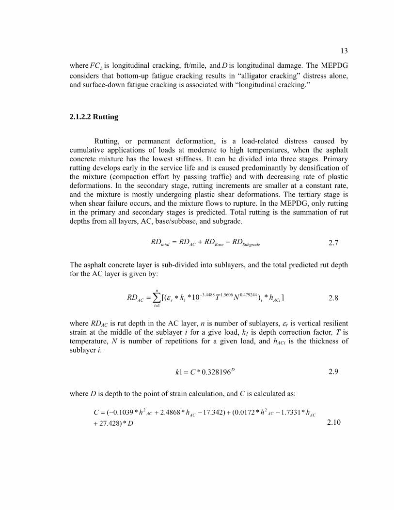
2.1.2.2 Rutting

Rutting, or permanent deformation, is a load-related distress caused by cumulative applications of loads at moderate to high temperatures, when the asphalt concrete mixture has the lowest stiffness. It can be divided into three stages. Primary rutting develops early in the service life and is caused predominantly by densification of the mixture (compaction effort by passing traffic) and with decreasing rate of plastic deformations. In the secondary stage, rutting increments are smaller at a constant rate, and the mixture is mostly undergoing plastic shear deformations. The tertiary stage is when shear failure occurs, and the mixture flows to rupture. In the MEPDG, only rutting in the primary and secondary stages is predicted. Total rutting is the summation of rut depths from all layers, AC, base/subbase, and subgrade.

The asphalt concrete layer is sub-divided into sublayers, and the total predicted rut depth for the AC layer is given by:

where RDAC is rut depth in the AC layer, n is number of sublayers, εr is vertical resilient strain at the middle of the sublayer i for a give load, k1 is depth correction factor, T is temperature, N is number of repetitions for a given load, and hACi is the thickness of sublayer i.

where D is depth to the point of strain calculation, and C is calculated as:

SubgradeBaseACtotal RDRDRDRD ++= 2.7

]*)10*[( 479244.05606.14488.31

1ACii

n

irAC hNTkRD −

=

∗= ∑ ε 2.8

DCk 328196.0*1 = 2.9

DhhhhC ACACACAC

*)428.27*7331.1*0172.0()342.17*4868.2*1039.0( 22

+−+−+−=

2.10

14

The MEPDG also divides all unbound granular materials into sublayers, and the total rutting for each layer is the summation of the rut depth of all sublayers. The predicted rut depth for the unbound granular base/subbase is as follows:

where RDG is rut depth in the unbound granular layer, β is calibration factor, a, b, and c are material properties, N is number of traffic repetitions, and hi is the thickness of sublayer i.

where Wc is percent water content, Er is resilient modulus of the unbound granular layer/sublayer, psi, and GWT is ground water table depth, ft. The calibration factors, β , for base/subbase and subgrade are 1.673 and 1.35, respectively.

2.1.2.3 Smoothness

The IRI over the pavement life depends on the initial as-constructed longitudinal profile of the pavement from which the initial IRI is computed and on the subsequent incremental development of distresses over time. These distresses include rutting, alligator cracking, longitudinal cracking, and thermal cracking for flexible pavements. In addition, smoothness loss due to soil movements and other climatic factors (depressions, frost heave, and settlement) are considered in the prediction of smoothness through the use of a “site factor” term (represented by a cluster based on foundation and climatic properties). The models for predicting IRI of flexible pavements with a granular base are a function of the base type as described below:

∑=

−=

n

iiv

Nb

G heaRDc

1

)(**][** εβ 2.11

cWc *017638.061119.0log −−= 2.12

215.0*log

)10/( 9 cc bb eea += 2.13

ccb /1

99 )

10189285.4(*10

−−

= 2.14

1192.0*3586.064.0/1 ])2555

[(*712.51 GWTrc

EW −= 2.15

15

where IRI is IRI at any given time, m/km, IRI0 is initial IRI, m/km, SF is site factor,

120 −age

e is age term (where age is expressed in years), COVRD is coefficient of variation of the rut depths, percent, TCLT is total length of transverse cracks at all severity levels, m, and FCT is fatigue cracking (alligator plus longitudinal) in the wheel path, percent of total lane area.

2.2 Pavement Instrumentation

Over the past several decades, attempts have been made to enhance pavement analysis and design by measuring the stresses, strains, and deflections inside a pavement structure and comparing them to calculated values from pavement response models. As technological capability advances, so does the entire supporting infrastructure system. Pavement instrumentation has recently become an important tool in monitoring in-situ pavement material performance and quantitatively measuring pavement response under different environmental and traffic conditions. Pavement instrumentation is not an objective but, rather, a tool to achieve specific goals. It is a process for monitoring the behavior of a specific pavement system. It comprises identification of critical locations in the pavement, selection of sensors, calibration of the sensors, identification of possible errors, installation, and, finally, data collection.

Typically, the pavement is instrumented so that both influencing factors and response parameters are measured quantitatively. Parameters that need to be measured in the field include, but are not limited to, strains, stresses, deflections, moisture, temperature, and traffic. Measuring these parameters in the field allows for the assessment of the major differences in the behavior of paving materials between laboratory and field conditions.

2.2.1 State-of-the-Art

A number of full-scale instrumented test sections have recently been incorporated into public highways. The MnRoad, Virginia Smart Road, Ohio National Test Road, and NCAT Test Track are prominent examples of this type of work. In addition, pavement instrumentation has been used extensively in a number of accelerated loading facilities to include those at the Federal Highway Administration and at sites in Louisiana, Kansas, California, and Nantes, France. In-situ pavement instrumentation is recognized as an important tool for the quantitative measurement of pavement response and performance.

TRD

LT

age

FCCOVTCeSFIRIIRI

*00384.0*1834.0*00119.0)]1(*[*0463.0 20

0

+++−+= 2.16

16

The major U.S instrumentation projects are discussed in the following subsections.

2.2.1.1 MnRoad

The Minnesota Road Research Project (MnRoad) includes a number of test pavements totaling 9.6 km in length. The site is located about 64 km northwest of Minneapolis/St. Paul. The test road with its sensor network and extensive data collection system has been used within the last decade to study how heavy commercial truck traffic and annual freeze/thaw cycles affect pavement materials and designs. Twenty-three of these test sections have been loaded with freeway traffic, and the remaining sections have been loaded with calibrated trucks. Freeway traffic loading began in June 1994. Embedded in the roadway are 4572 electronic transducers, 1151 of which are used to measure pavement response to dynamic axle loading (Baker 1994). In addition, three of the MnRoad cells were reconstructed in 1999, with Superpave mixes containing three different binders. The sites were instrumented, and their performance and response were measured.

2.2.1.2 Virginia Smart Road

The Smart Road is a 9.6-km connector highway between Blacksburg and I-81 in southwest Virginia, with the first 3.2 km designated as a controlled test facility. The flexible pavement portion of the Virginia Smart Road includes 12 different flexible pavement designs (Loulizi et al. 2001). Each section is approximately 100 m long. Seven of the 12 sections are located on a fill, while the remaining five sections are located in a cut. All 12 sections are closely observed through a complex array of sensors located beneath the roadway and embedded during construction. The Smart Road is unique in many aspects, including having all pavement layers instrumented for monitoring the effects of loading and the environment. Pavement materials can be tested under different environmental conditions using the All Weather Testing facility. In addition to the flexible pavement test sections, a continuously reinforced rigid pavement is included.

2.2.1.3 Ohio National Test Road

The Ohio Department of Transportation, in cooperation with the Federal Highway Administration, constructed a 5-km-long test pavement on U.S. 23 north of Delaware, Ohio. This project encompasses four experiments identified in the Specific Pavement Studies (SPS) of the LTPP program and includes 40 test sections of asphalt and portland cement concrete (PCC) with a variety of structural parameters (Sargand et al.

17

1997). All of the test sections were constructed as part of one project in which the climate, soil, and topography were uniform throughout. The test sections were instrumented with various devices. Response data were collected for various axle configurations, loads, and types of tires, and, traveling over a range of speeds, passed over specific test sections. Environmental data were periodically collected throughout the year to better define the effect of seasonal variations on pavement structures and continuously during the controlled vehicle tests to properly interpret the response of pavement sections under actual truck loading. The main objective of the Ohio National Test Road was to do a long-term study of structural factors, maintenance effectiveness, rehabilitation, and environmental factors on the mechanistic response of various pavement sections. Of particular interest is the interaction of load response to environmental parameters.

2.2.1.4 NCAT Test Track

This project includes eight asphalt concrete pavement sections that were constructed at the NCAT test track (Timm et al. 2004). These sections varied in thickness and material composition. Additionally, each of the sections was instrumented to monitor in-situ asphalt strain, compressive stresses in the unbound layers, moisture, and temperature. Throughout the course of the experiment, data were gathered both in a slow speed manner in addition to a high-speed dynamic manner under normal operating speeds. Additionally, routine deflection testing and surface condition surveys were conducted.

2.2.2 Application of Instrumentation Data

In general, there are two major applications of pavement instrumentation data. The first type of application is used to validate existing or novel design approaches. This is accomplished by verifying field-measured parameters with theoretically calculated parameters. For instance, measuring stresses and strains in the field and then comparing them to their calculated counterpart in a pavement response model may serve this application. The second type of application is used to identify trends in measured parameters that may indicate the health of a pavement structure. Monitoring deflections at different locations in a pavement may yield information on how pavements deteriorate with time and accordingly assist in the second application. Considering the scope of this thesis research, several examples of the first type of application are provided in this section.

In 1999, an AC pavement section was instrumented on County Road K52 in Sioux County, Iowa. Both dynamic and environmental sensors were installed during construction to measure strains, temperature, and moisture. The sensors were attached to the top of the first lift, or about 75 mm up from the subgrade, and under the wheel path. The pavements were tested at low speeds, less than 8 kph, under vehicle-of-husbandry

18

and standard-truck loads. Fanous et al. compared the strain responses predicted from a multi-layer elastic analysis program, KENLAYER, to those obtained from the field test. Some discrepancies between the analytical and the field test results were noticed. These most likely were due to the uncertainty of the values of the parameters, such as the soil subgrade reaction, and the actual elastic modulus and the thickness of the pavement. In spite of this discrepancy, both analytical and field test results revealed similar behaviors for the pavement.

Wu and Hossain (2003) used a multi-layer elastic analysis program, ELSYM5, to validate measured pavement responses. Instrumentation sections were constructed at the Kansas Accelerated Testing Laboratory (K-ATL) with 12.5-mm nominal maximum size Superpave mixtures (SM-2A) with varying percentages (15 and 30 percent) of river sand. A 150-kN tandem axle with dual wheels was used for 10,000 repetitions. The sections were then loaded by three different tandem axle loads and three single axles for more than 30 repetitions in each configuration to estimate the relative pavement damage in the SM-2A layer due to different axle loads and configurations. All load applications were done at a temperature of approximately 38oC at the middle of the SM-2A layer. The test sections were instrumented at three locations on each test section with transverse strain gauges at the bottom of the SM-2A layer, pressure cells on the top of the subgrade, and temperature gauges in the aggregate base, subgrade, and SM-2A layers (mid-depth and bottom). Response data were collected during load applications by the K-ATL tandem axle and a Falling Weight Deflectometer (FWD). The authors reported that the measured vertical stresses on the top of the subgrade and tensile strains at the bottom of the SM- 2A layer due to FWD loads are generally very close to those calculated by a multi-layer elastic analysis program, ELSYM5. However, measured tensile strains and vertical stresses on both sections were higher than those calculated by ELSYM5. In general, the measured tensile strains under the K-ATL wheel loads were found to increase with increasing number of wheel load repetitions, but the measured vertical stresses remained relatively constant.

Bao (2000) computed the “ratio” of field-measured strains to predicted strains from a multi-layer elastic analysis program, WESLEA. Based on the instrumentation data from MnRoad, graphs were first developed to illustrate the effects of axle load, speed, tire pressure, offset, layer modulus, and layer thickness on this “ratio.” A commercially available statistics software package, SPSS, was used to estimate the mathematical relationships between the “ratio” and each affecting parameter separately and then to determine the complete “ratio” model including all the parameters using nonlinear regression analysis on a large set of testing data. Finally, a randomly selected set of data was used to validate the calibrated structural model incorporated in WESLEA. The author concluded that the pavement response can be accurately predicted in terms of horizontal strain at any point for any flexible pavement structure under certain load configurations by magnifying the WESLEA prediction with a “ratio” factor.

Elseifi et al. (2006) presented a comprehensive validation study on pavement response. The research objective was to characterize HMA viscoelastic properties at intermediate and high temperatures and to incorporate laboratory-determined parameters into a 3-D FE model in order to accurately simulate pavement responses to vehicular loading at different temperatures and speeds. Results of the developed FE model were

19

compared against field-measured pavement responses from the Virginia Smart Road. Results of this analysis indicated that the elastic theory grossly under-predicts pavement responses to vehicular loading at intermediate and high temperatures. In addition, the elastic FE model could not simulate permanent deformation or delayed recovery. In contrast, results of the FE viscoelastic model were in better agreement with field measurements. The FE model successfully simulated retardation of the response in the transverse direction and rapid relaxation of HMA in the longitudinal direction.

2.3 Deterministic Approach vs. Probabilistic Approach

Performance prediction is a complex process that involves many uncertainties, variabilities, and approximations. Perhaps the most obviously uncertain of all is estimating climate condition many years into the future. Materials and traffic also introduce a measure of variability. Even though mechanistic concepts provide a more rational and realistic methodology, a consistent and practical method for considering these uncertainties and variations is needed so that the best possible representation of the pavement performance can be reflected.

The most common type of performance model is a deterministic model. Deterministic models use discrete input values that represent the "best guess" of each parameter. For instance, one deterministic model can use regression analysis to predict a single value of pavement condition from one or more parameters (e.g., material properties and traffic). The inherent variability associated with each input parameter is not included in the model or accounted for by inflating or deflating the “best guess” and therefore is not reflected in the model results. Accounting for the uncertainty of input parameters in the performance model is extremely complicated. A sensitivity analysis is often performed in order to assess the effects of various input parameters on the model results; however, the sensitivity analysis does not necessarily reveal areas of uncertainty that may be a critical part of the performance prediction process. Unfortunately, the performance prediction models presented in the MEPDG are still deterministic models even though the reliability concept is applied. From a pavement design perspective, the reliability of a pavement design can be thought as a safety factor that is used to ensure the pavement will perform its intended function over its design life (or time) and under the conditions (or environment) encountered during operation.

Obviously, it is desirable to include uncertainties in performance models so that the pavement engineers can weigh the probability of any particular outcome that may occur, as illustrated in the following general form:

where P is the pavement performance, Xi’s are the parameters required for the performance model, and e is the error term related to several sources of variability. One major source of variability is the measurement error. Since most performance models

( ) eXXXfP += ,...,, 321 2.17

20

today are either empirical or empirical-mechanistic in nature, another major source of variability is attributed to error in predicting performance. This source of uncertainty is commonly known as model uncertainty. As the performance model becomes more mechanistic, the model-based uncertainties will become smaller. An ideal performance model should combine probabilistic descriptions of input parameters with specific simulation techniques to characterize the probabilistic characteristics associated with possible outcomes (Yin et al. 2002). One such simulation technique is Monte Carlo (MC) simulation. MC simulations are stochastic techniques, meaning that they are based on the use of random numbers and probability statistics to investigate problems. MC simulations randomly select values to create scenarios of a problem. The random selection process is repeated many times to create multiple scenarios. Each time a value is randomly selected, it forms one possible scenario and solution to the problem. Together, these scenarios give a range of possible solutions, some of which are more probable and some less probable.

Probabilistic modeling exposes areas of uncertainty that may be hidden in a deterministic model and allows the pavement engineers to predict the probability of a specific outcome. A comparison of deterministic and probabilistic analyses is graphically shown in Figure 2.2.

2.4 Summary

In the recent decades, researchers have been actively investigating the applications of pavement instrumentation data. However, trivial work has been accomplished in the area of utilizing instrumentation data for performance predictions. Given the uncertainties associated with design parameters, a probabilistic-based approach

Several values simulated One value per construction

distribution per input single value per input

Deterministic Analysis Probabilistic Analysis

One Value per single value per output distribution per output

Several values simulated One value per construction

distribution per input single value per input

Deterministic Analysis Probabilistic Analysis

One Value per single value per outputOne Value per single value per output distribution per output distribution per output

Figure 2.2: Comparison of deterministic and probabilistic analyses

21

is essential for accurate performance predictions. It is hoped that this thesis research will serve as a first step in the probabilistic performance prediction of flexible pavements using instrumentation data.

Chapter 3

The SISSI Project

3.1 Background

Immediately after the introduction of Superpave, various technology transfer means were utilized to implement the new mix design procedure. In the late 1990s, PennDOT made a commitment to move to Superpave designs in order to improve flexible pavement performance. The newly released Mechanistic-Empirical Pavement Design Guide (MEPDG) is compatible with the Superpave system and, consequently, will make new and more sophisticated technology available to the pavement engineer and, in particular, to the construction industry and to user agencies. Using this method, the engineer will arrive at a final HMA mix design by considering structural, traffic, and environmental factors in addition to material properties, thus fulfilling the original goal of the 1993 SHRP mix design and analysis method. The accuracy of performance prediction models depends on an effective process of calibration and subsequent validation with independent data sets. Pavement engineers need to see an acceptable correlation between field-observed levels of permanent deformation, fatigue cracking, and low-temperature cracking and levels predicted with the hot-mix asphalt (HMA) performance models selected for use in structural and mix design. Such accuracy is also important if the results of these models are to be used in the development of performance-related specifications. Performance prediction models incorporated into the MEPDG must be refined and validated for use at the state level.

In 2001, the Pennsylvania Department of Transportation (PennDOT) initiated a major five-year research program titled “Superpave In-Situ Stress/Strain Investigation (SISSI).” This project includes eight pavement sites throughout the Commonwealth of Pennsylvania. A large amount of dynamic (load-associated) sensors and environmental (non-load) sensors were instrumented during pavement construction, with the least interference to common and normal paving operations. Each site was also equipped with a weigh-in-motion (WIM) station for traffic data collection (Stoffels and Solaimanian 2003).

3.2 Objectives

The SISSI project is an innovative pavement instrumentation project. It is designed to provide pavement performance data that can be used to establish the performance and to develop life-cycle cost data for full-depth asphalt pavements and

23

portland cement concrete pavements with asphalt concrete overlays. Data collected from the project will also provide the data required for the calibration and validation of pavement performance models.

3.3 Site Selection

One of the most labor-intensive tasks of the SISSI project was selection and instrumentation of pavement sites. The idea was to select sites that would satisfy required environmental and traffic data and at the same time be proper candidates for instrumentation. It was decided that sites would be selected in both the northern and southern parts of the Commonwealth (north of I-80 and south of I-80) to represent the temperature difference as well as the difference in the freeze-thaw cycles the pavement undergoes during the winter-spring time period. It was also decided that two types of pavement construction would be included: 1) full-depth structure including subbase, base, and Superpave-designed hot-mix asphalt layers constructed over the subgrade and 2) structural overlay including only Superpave-designed hot-mix asphalt layers. The term “structural” was used to distinguish these mixes from maintenance overlay mixes (Solaimanian et al. 2006). The locations of the final selected pavement sites are presented in Figure 3.1.

Figure 3.1: Counties with SISSI instrumentation sites

24

3.4 Pavement Construction

The first pavement section selected for this study was a full-depth AC pavement section on the southbound lane of U.S. SR 1001 in Blair County, Pennsylvania. The construction of this section was completed in the fall of 2003. This pavement section consisted of a granular 2A subbase and three Superpave-designed hot-mix asphalt layers: a bituminous concrete base course (BCBC), a binder course, and a wearing course. The second pavement section selected for this study was a structural overlay AC pavement section on the eastbound lane of U.S. SR 0006 in Warren County, Pennsylvania. The construction of this section was completed in the fall of 2001. This pavement section consisted of four Superpave-designed hot-mix asphalt layers over a cracked and seated concrete pavement: a leveling course, a BCBC, a binder course, and a wearing course. Both sites were constructed with PG 64-22 asphalt binder. Tables 3.1 and 3.2 provide a summary of the types of pavement structures at the Blair and Warren sites, respectively. Details of the SISSI pavement structure and construction are provided in the project construction reports (Solaimanian et al. 2006).

Table 3.1: Construction information for Blair

Layer Thickness, mm Binder PG Nominal Maximum Aggregate Size (NMAS), mm

Wearing 54 64-22 12.5 Binder 47 64-22 19.0 BCBC 162 64-22 25.0

Subbase 200 - -

Table 3.2: Construction information for Warren

Layer Thickness, mm Binder PG Nominal Maximum Aggregate

Size (NMAS), mm Wearing 38 64-22 9.5 Binder 62 64-22 25.0 BCBC 138 64-22 37.5

Leveling 110 64-22 25.0 Fractured PCC 250 - -

25

3.5 Pavement Instrumentation

Instrumentation of the pavement layers was an integral part of this project, the details of which are reported in a project instrumentation report (Anderson et al. 2003). Both load-associated and environmental transducers were installed at different layers. Two replicate locations were instrumented at each of the eight SISSI sites. The number and location of the transducers varied according to the pavement structure at each site, as summarized in Table 3.3. Detailed transducer layout can be found in Appendix A. Cables buried in the pavement connected the transducers to an instrumentation cabinet at the edge of the shoulder. The instrumentation cabinet contained the data logger used for the environmental measurements and a modem for transmitting data.

The load-associated and environmental transducers were installed in the travel lane. The load-associated transducers were either in or immediately adjacent to the right wheel path, while the environmental transducers were placed at the center of the travel lane, between the wheel paths, where they would be least affected by the wheel loads. Environmental data were collected frequently and remotely through modems installed at the sites. Load-associated responses were collected at different times of the year to capture the seasonal effects under controlled loading conditions. Transducers installed to capture the pavement response under truck loading included pressure cells and strain gauges in the unbound layers, H-type strain gauges in asphalt layers, and multi-depth deflectometers (MDD) throughout all the pavement layers. All gauges except MDD’s were installed in the horizontal direction. Pressure cells and strain gauges are presented in Figure 3.2.

Table 3.3: Number of dynamic transducers installed at different SISSI sites

Site Location HMA Strain Gauge

Unbound Layer Strain Gauge

Multi-Depth Deflectometer

Pressure Cell

1 10 0 0 0Warren 2 10 0 0 0

1 10 4 2 4Blair 2 10 4 2 4

26

The principal sources of in-situ environmental data at the test sites were thermocouples for temperature measurement, time-domain reflectometers for moisture content measurement, and resistivity probes for frost depth measurements. In 2004, Campbell Scientific pyranometers were installed at SISSI sites to capture solar radiation; however, only pavement temperature data collected during the SISSI project were used in this study. Table 3.4 presents the environmental transducers installed at different SISSI sites.

(a) Pressure Cell (b) Strain Gauge in Unbound (c) Strain Gauge in AC

Layers Layers

Figure 3.2: Dynamic transducers installed at SISSI sites

Table 3.4: Number of environmental transducers installed at different SISSI sites

Site Location Thermocouple Moisture Probe Frost Probe Pyranometer

1 3 0 0 0Warren 2 9 0 1 1

1 12 4 1 1Blair 2 11 4 1 0

27

3.6 Data Collection

3.6.1 Material Characterization Data

During Phase I of the SISSI project, significant effort was made to characterize the binders and mixtures used at all instrumented sites (Solaimanian et al. 2006). The following tests were the primary tests conducted for the binder characterization:

Rotational Viscometer (RV) Dynamic Shear Rheometer (DSR) Bending Beam Rheometer (BBR)

The tests on mixtures included tests on the loose mixture as well as tests on the compacted specimens. The tests on the loose mixture included determination of the maximum theoretical specific gravity and determination of binder content and aggregate gradation. The tests on the compacted specimens included determination of the bulk specific gravity and complex modulus tests.

3.6.2 Instrumentation Data

Load-associated pavement response is captured through application of controlled loads at certain speeds using a specialty truck (Anderson and LeBoon 2002). Different speeds and different load configurations were used for this purpose. The tractor trailer was equipped with moveable concrete blocks so that the distribution of load on different axles could be controlled (Figure 3.3). The pavement responses were measured at different vehicle speeds under different load configurations (front or back) as each of the four axles passes the instrumented sections. Truck speeds included 8, 16, 32, 64, and 96 kilometers per hour (kph). Dynamic data were collected by a specific data acquisition system at multiple times of the year to capture the seasonal effects. Measurement of environmental data was conducted on a continuous basis, and the resulting data were acquired by permanently installed data loggers that were connected to the server at the Pennsylvania State University via land lines or cell phone service.

28

3.6.3 Traffic Data

The SISSI project undertook the collection of traffic data at each pavement test location as a part of the information-gathering process (Stoffels et al. 2006). Weigh-in-motion (WIM) equipment was installed by PennDOT adjacent to each pavement test location in order to collect traffic information on-site. Weigh-in-motion is a process of measuring the dynamic tire forces of a moving vehicle and estimating the corresponding tire loads of the static vehicle. Gross-vehicle weight of a highway vehicle is due only to the local force of gravity acting upon the composite mass of all connected vehicle components and is distributed among the tires of the vehicle through connectors such as springs, motion dampers, and hinges. The WIM System has a set of sensors and supporting instruments that measure the presence of a moving vehicle and the related dynamic tire forces at specified locations with respect to time, estimate tire loads, calculate speed, axle spacing, vehicle class according to axle arrangement, and other parameters regarding the vehicle, and process, display, store, and transmit this information. Traffic data were collected utilizing PAT America piezo WIM systems.

3.6.4 Climate Data

The primary sources of site-specific data were the PennDOT Road Weather Information System (RWIS) sites. This data was supplemented by data from the Department of Environmental Protection and national weather data. PennDOT currently operates approximately 80 RWIS sites across the Commonwealth that report temperature,

Figure 3.3: Truck with moveable weights for pavement loading

29

wind data, relative humidity, dew point, visibility, precipitation data, and specific roadway conditions. These sites have been installed for the principal purpose of maintenance management to avoid adverse surface conditions during winter weather; however, the stations also provide a valuable source of site-specific weather data, and some sites were installed adjacent to the SISSI sites. PennDOT provides weather data to the Penn State Meteorology department, where it is included in the Mesonet. The nearest RWIS site was designated as the primary weather data collection site. In several cases, there were multiple RWIS sites within a reasonably close distance from the test locations. In these instances, the site considered to be most representative of the test location was selected, considering elevation and intervening geographic features. In cases where the primary RWIS site was not operational for some period of time, other nearby sites were considered as backup sources of information. The locations of SISSI weather stations are shown in Figure 3.4. The SISSI climate data include temperature, wind, cloud cover, and solar radiation data (Stoffels et al. 2006).

3.6.5 Falling Weight Deflectometer Data

As is commonly known, laboratory results do not directly translate into calibrated predictions of field results; field correlations are necessary. For example, when laboratory-derived material moduli are used in layered elastic or finite element analysis, stresses, strains, and deflections are often significantly over-predicted. Therefore, falling weight deflectometer (FWD) testing was conducted on each of the SISSI locations periodically because measured deflections provide a step in developing the relationships between laboratory and field measurements (Stoffels et al. 2006). For the SISSI project, all FWD tests were performed by PennDOT. The FWD tests were performed for each wheel path and centered between wheel paths. The deflection data were collected during construction and during different seasons.

30

3.6.6 Performance Data

This section presents a general overview of the performance data collection for the SISSI project (Stoffels and Solaimanian 2006). Distress summaries and International Roughness Index (IRI) were extracted from PennDOT’s Roadway Information Management System for each segment containing an instrumented pavement section. These data were collected to allow for the comparison of the instrumented sections to the overall construction so that the analysis was not unduly influenced by any distresses induced or partially induced by the instrumentation. The pavement performance data in the roadway management system were collected by a vendor. The vendor used a videologging system for the collection of the distress data and an inertial profile for the collection of the longitudinal profile.

Figure 3.4: Locations of SISSI weather stations

31

Manual distress surveys were conducted in accordance with Long Term Pavement Performance (LTPP) protocols. Distress surveys were conducted over one-thousand-foot sections, including both instrumentation sections. Detailed crack maps were prepared for each instrumentation section. Photographs were taken in conjunction with the manual distress surveys. These digital photographs were stored with the project data.

Initial profiles on each site were collected using rod- and level-type surveys, as summarized in the construction reports. Afterward, the performance monitoring continued with the transverse profiler developed for the SISSI project. Transverse profiles for SISSI sites were captured every time the crew conducted dynamic measurements at the sites. In some cases, due to time constraints, no transverse profile was obtained, and only dynamic measurements were conducted; in other cases, only one location at each site was subject to transverse profiling.

Chapter 4

Preliminary Data Analysis

4.1 Introduction

The SISSI Project is a comprehensive project that includes a wide spectrum of activities directed toward the validation of the Superpave system and the corresponding performance prediction models. The central part of these activities is successful collection of various types of data from the instrumented sites. The data collected from the SISSI project can be briefly classified as follows:

Traffic data from weigh-in-motion sensors installed at the sites Environmental data from measurements at the instrumented sites and

from PennDOT RWIS Pavement response data under controlled and uncontrolled truck

loading Data from falling weight deflectometer (FWD) measurements Materials characterization data of AC Pavement condition data Construction data

This chapter deals with presentation and preliminary analysis of the first five classes of the preceding data types. The last two classes of the SISSI data will be presented along with individual research tasks.

4.2 Traffic Data

Consideration of traffic loading information is one of the most important elements of a successful pavement design. Traffic loads, along with the environment, damage pavement over time. Traditionally, the expected loads a pavement will encounter over its design life have been quantified through the equivalent single axle load (ESAL) approach, which converts axle loads of various magnitudes and repetitions (mixed traffic) to an equivalent number of standard loads. Equivalency factors are used to determine the number of ESALs for each axle load and axle configuration. These factors are based on the present serviceability index concept and depend on the pavement type and structure. Studies have shown that these factors theoretically should be influenced by pavement condition, distress type, failure mode, and other parameters.

Mechanistic-empirical pavement design procedures consider the response of pavement materials to applied loads. For highways, these are wheel loads; therefore, it is

33

important to accurately consider the effects of wheel loads of individual vehicles and account for cumulative damage resulting from repeated loading. The MEPDG does this in the form of load spectra, a catalog of each wheel load, including size and weight. Load repetitions are estimated by extrapolating historical trends or applying other growth projections. As presented in the following sections, the analysis of traffic data is primarily focused on processing the data into the load spectrum necessary for the MEPDG applications.

4.2.1 General Information

Based on the volume of traffic data collected by site-specific WIM at Blair (years 2004-2006) and Warren (years 2002-2006), general traffic information is summarized in Table 4.1. Two-way average annual daily truck traffic (AADTT) is the total volume of truck traffic, the total number of heavy vehicles (FHWA vehicle classes 4 to 13, as seen in Figure 4.1) in the traffic stream, passing a point or segment of a road facility to be designed in both directions during a 24-hour period. FHWA vehicle classifications are as follows (FHWA 2001):

Class 1. Motorcycles – All two- or three-wheeled motorized vehicles. Typical vehicles in this category have saddle-type seats and are steered by handlebars rather than steering wheels. This category includes motorcycles, motor scooters, mopeds, motor-powered bicycles, and three-wheel motorcycles.

Class 2. Passenger Cars – All sedans, coupes, and station wagons manufactured primarily for the purpose of carrying passengers, including those passenger cars pulling recreational or other light trailers.

Class 3. Other Two-Axle, Four-Tire Single Unit Vehicles – All two-axle, four-tire vehicles other than passenger cars. Included in this classification are pickups, panels, vans, and other vehicles such as campers, motor homes, ambulances, hearses, carryalls, and minibuses.

Class 4. Buses – All vehicles manufactured as traditional passenger-carrying buses with two axles and six tires or three or more axles. This category includes only traditional buses (including school buses) functioning as passenger-carrying vehicles.

Class 5. Two-Axle, Six-Tire, Single-Unit Trucks – All vehicles on a single frame, including trucks, camping and recreational vehicles, motor homes, etc., with two axles and dual rear wheels.

Class 6. Three-Axle Single-Unit Trucks – All vehicles on a single frame, including trucks, camping and recreational vehicles, motor homes, etc., with three axles.

Class 7. Four or More Axle Single-Unit Trucks – All trucks on a single frame with four or more axles.

34

Class 8. Four or Fewer Axle Single-Trailer Trucks – All vehicles with four or fewer axles consisting of two units, one of which is a tractor or straight truck power unit.

Class 9. Five-Axle Single-Trailer Trucks – All five-axle vehicles consisting of two units, one of which is a tractor or straight truck power unit.

Class 10. Six or More Axle Single-Trailer Trucks – All vehicles with six or more axles consisting of two units, one of which is a tractor or straight truck power unit.

Class 11. Five or Fewer Axle Multi-Trailer Trucks – All vehicles with five or fewer axles consisting of three or more units, one of which is a tractor or straight truck power unit.

Class 12. Six-Axle Multi-Trailer Trucks – All six-axle vehicles consisting of three or more units, one of which is a tractor or straight truck power unit.

Class 13. Seven or More Axle Multi-Trailer Trucks – All vehicles with seven or more axles consisting of three or more units, one of which is a tractor or straight truck power unit.

Percent trucks in the design direction is used to quantify any difference in the overall volume of trucks in two directions. Because of the arrangement of WIM set-up, this information is not available at Warren, but it can be reasonably assumed to be 50 percent as recommended by the MEPDG. Percent trucks in the design lane accounts for the distribution of truck traffic between the lanes in one direction. For two-lane, two-way highways (one lane in one direction), this percentage is 100 because all truck traffic in any one direction must use the same lane. There were two lanes in the design direction, with 91 percent and 79 percent of the trucks in the design lane for Warren and Blair, respectively.

35

Table 4.1: General traffic information

Blair Warren AADTT Trucks, % AADTT Trucks, % Year Da Lb D L D L Dc L

2002 - - - - 479 432 - 90 2003 - - - - 456 418 - 92 2004 153 88 56 78 322 284 - 88 2005 174 122 47 79 424 386 - 91 2006 175 133 43 80 428 392 - 92

a Design direction b Design lane c Information is not available

Figure 4.1: Illustrations and definitions of the vehicle classes (FHWA 2001)

36

4.2.2 Vehicle Operational Speed

The vehicle operational speeds of trucks, or the average travel speed, generally depends on many factors, including the roadway facility type (Interstate or otherwise), terrain, and percentage of trucks in the traffic stream. As plotted in Figure 4.2, unlike Warren, the operational speed at Blair was slightly lower in the first 12 months and then became stable.

4.2.3 Traffic Growth Factor

Traffic growth factors at a particular site or segment are best estimated when continuous AADTT data is available (assuming that the data are reliable and that the differences found from year to year can be attributed to growth) since it is well known that traffic volumes at a single site can be affected by a variety of extraneous factors, and thus growth factors computed from limited data collected from a limited number of locations can be biased. In this study, trend analysis was used as a methodology for forecasting future truck volumes that relies solely on historical AADTT after the base year. While it is theoretically possible to develop trends of volumes from only 2 years of data (as for Blair), more data points are desirable so that the impacts of non-representative data points can be minimized. The simplest form of trend analysis is a linear regression method that forecasts future truck volumes based solely on historical truck volumes, developing a trend line of volumes into the future. As shown in Figure 4.3, no apparent traffic growth was observed at Warren, while there was an apparent linear relationship between time and traffic volume at Blair. The linear increase corresponds to a growth factor of 8 percent.

90

92

94

96

0 5 10 15 20 25 30 35 40 45 50 55Month

Ave

rage

Spe

ed, k

ph

64

66

68

70

72

0 5 10 15 20 25 30 35Month

Ave

rage

Spe

ed, k

ph

(a) Warren (b) Blair

Figure 4.2: Vehicle operational speeds

37

4.2.4 Vehicle Class Distribution

Normalized vehicle class distribution represents the percentage of each truck class within the AADTT. The sum of the percent AADTT of all truck classes should equal 100. Averaged vehicle class distributions over the past years are shown in Figure 4.4; the dominant vehicle classes are 5 and 9 for both the Warren and Blair sites.

3800

4000

4200

4400

2003 2004 2005 2006

Year

Tra

ffic

Vol

ume,

AA

DT

T

8200

8400

8600

8800

2004 2005 2006

Year

Tra

ffic

Vol

ume,

AA

DT

T


Figure 4.3: Determination of traffic growth factors

0

20

40

60

4 5 6 7 8 9 10 11 12 13

Vehicle Class

Perc

enta

ge o

f Tru

ck T

raff

ic, % 2002

2003200420052006

0

20

40

60

4 5 6 7 8 9 10 11 12 13

Vehicle Class

Perc

enta

ge o

f Tru

ck T

raff

ic, % 2004

20052006


Figure 4.4: Vehicle class distributions

38

4.2.5 Monthly Adjustment Factor

Truck traffic monthly adjustment factors represent the proportion of the annual truck traffic for a given truck class that occurs in a specific month. In other words, the monthly distribution factor for a specific month is equal to the monthly truck traffic for the given class for the month divided by the total truck traffic for that truck class for the entire year. Truck traffic monthly adjustment factors (MAF) depend on factors such as adjacent land use, the location of industries in the area, and roadway location (urban or rural). In reality, monthly differences in the truck traffic distribution could vary over the course of several years during the pavement life. MAF is site-specific as well as highly dependent on the local economy and climatic conditions. MAF of two dominant vehicle classes, 5 and 9, are plotted in Figure 4.5 and Figure 4.6 for Warren and Blair, respectively. Except for the year 2004 at Warren, the seasonal effect on the AADTT occurring over a 24-hour period of each month is minimal.

0.0

0.5

1.0

1.5

2.0

Janu

ary

Febr

uary

Mar

ch

Apr

il

May

June

July

Aug

ust

Sept

embe

r

Oct

ober

Nov

embe

r

Dec

embe

r

Month

Mon

thly

Adj

ustm

ent F

acto

r

2002 2003 20042005 2006

0.0

0.5

1.0

1.5

2.0

Janu

ary

Febr

uary

Mar

ch

Apr

il

May

June

July

Aug

ust

Sept

embe

r

Oct

ober

Nov

embe

r

Dec

embe

r

Month

Mon

thly

Adj

ustm

ent F

acto

r2002 2003 20042005 2006

(a) Class 5 (b) Class 9

Figure 4.5: Monthly adjustment factors for Warren

0.0

0.5

1.0

1.5

2.0

Janu

ary

Febr

uary

Mar

ch

Apr

il

May

June

July

Aug

ust

Sept

embe

r

Oct

ober

N

ovem

ber

Dec

embe

r

Month

Mon

thly

Adj

ustm

ent F

acto

r

2004 2005 2006

0.0

0.5

1.0

1.5

2.0

Janu

ary

Febr

uary

Mar

ch

Apr

il

May

June

July

Aug

ust

Sept

embe

r

Oct

ober

N

ovem

ber

Dec

embe

r

Month

Mon

thly

Adj

ustm

ent F

acto

r

2004 2005 2006

(a) Class 5 (b) Class 9

Figure 4.6: Monthly adjustment factors for Blair

39

4.2.6 Hourly Truck Distribution

The hourly distribution factors (HDF) represent the percentage of the AADTT within each hour of the day. The sum of the percent of daily truck traffic per time increment must add up to 100 percent. Hourly truck distributions are shown in Figure 4.7. The Warren and Blair sites exhibit a similar bell-shaped distribution. In addition, most of the truck traffic occurs from 5 a.m. to 3 p.m. During this 10-hour period, the hourly truck traffic accounts for more than 50 percent of the AADTT.

4.2.7 Axle Load Distribution

The axle load distribution factors simply represent the percentage of the total axle applications within each load interval for a specific axle type (single, tandem, tridem, and quad) and vehicle class (classes 4 through 13). A definition of load intervals for each axle type is provided below:

Single axles – 1361 kg to 18144 kg at 454-kg intervals Tandem axles – 2722 kg to 36287 kg at 907-kg intervals Tridem and quad axles – 5443 kg to 46266 kg at 1361-kg intervals

An example of single axle load distribution at Warren is given in Table 4.2.

0

2

4

6

8

10

0 4 8 12 16 20Hour

Hou

rly

Tru

ck D

istr

ibut

ion,

%

0

2

4

6

8

10

0 4 8 12 16 20Hour

Hou

rly

Tru

ck D

istr

ibut

ion,

%


Figure 4.7: Hourly truck distribution

40

Table 4.2: Single axle load distribution at Warren

Interval Class 4 Class 5 Class 6 Class 7 Class 8 Class 9 Class 10 Class 11 Class 12 Class 131 0 1.02 0 0 0.5 1.41 0.11 0.99 0 1.522 0.54 18.4 0.3 0.05 1.76 3.49 0.7 5.46 6.25 03 1 11.02 0.54 0.11 2.4 2.16 1.11 14.52 31.25 5.614 5.93 11.18 1.25 0.61 5.95 1.69 0.9 16.79 18.75 05 18.01 11.71 2.61 1.33 9.95 6.37 5.9 9.94 0 6.366 10.26 10.5 6.9 1.72 16.94 25.5 19.3 11.33 6.25 12.517 9.36 7.79 14.72 2.96 16.44 22.18 30.67 11.51 10.42 38.888 11.44 6.39 18.16 4.34 11.53 16.86 25.26 7.71 8.33 4.099 13.16 5.07 12.32 6.35 8.42 8.12 9.83 3.53 4.17 8.6610 8.51 3.67 13.06 9.32 6.04 2.21 4.42 3.44 0 1.8211 5.83 2.62 11.22 10.58 5.38 0.77 0.85 3.51 2.08 012 5.98 2.11 7.74 11.35 3.79 0.72 0.28 2.44 4.17 3.5713 4.23 1.64 4.24 12.34 3 0.95 0.16 2.45 2.08 3.0314 2.44 1.36 2.11 11.76 2.25 1.3 0.14 2.48 0 015 1.13 1 1.99 10.04 1.76 1.6 0.14 1.26 0 016 0.45 0.76 1.26 7.04 1.21 1.75 0.14 1 4.17 3.0317 0.5 0.62 0.68 4.96 0.87 1.35 0 0.83 0 1.318 0.43 0.5 0.4 2.99 0.54 0.82 0 0.24 0 3.7919 0.32 0.45 0.28 1.52 0.55 0.4 0 0.47 2.08 020 0.1 0.42 0.13 0.5 0.32 0.2 0 0 0 2.2721 0.1 0.35 0.05 0.13 0.13 0.07 0 0 0 022 0.16 0.34 0.02 0.02 0.05 0.03 0 0.13 0 023 0.04 0.27 0.01 0 0.06 0.01 0 0 0 2.2724 0.07 0.26 0.01 0 0.03 0.01 0.1 0 0 025 0 0.19 0 0 0.06 0 0 0 0 026 0.02 0.15 0 0 0.01 0 0 0 0 027 0 0.08 0 0 0.04 0 0 0 0 028 0 0.07 0 0 0.01 0 0 0 0 1.329 0 0.03 0 0 0.01 0 0 0 0 030 0 0.03 0 0 0.01 0 0 0 0 031 0 0.01 0 0 0 0 0 0 0 032 0 0.01 0 0 0 0 0 0 0 033 0 0 0 0 0 0 0 0 0 034 0 0 0 0 0 0 0 0 0 035 0 0 0 0 0 0 0 0 0 036 0 0 0 0 0 0 0 0 0 037 0 0 0 0 0 0 0 0 0 038 0 0 0 0 0 0 0 0 0 039 0 0 0 0 0 0 0 0 0 0

41

4.2.8 Number of Axles per Truck Class

The number of axles per truck class represents the average number of axles for each truck class (class 4 to 13) for each axle type (single, tandem, tridem, and quad). An example of single axle load distribution at Blair is given in Table 4.3.

4.3 Climate Data

4.3.1 General Analysis of Temperature Data

During the SISSI project, various types of environmental data were collected through non-load-associated environmental sensors and the nearest RWIS weather stations. These data included air temperature, relative humidity, cloud cover, precipitation, pavement temperature, solar radiation, volumetric water content, and frost depth. Because of the scope of this study, the analysis presented here is mainly focused on pavement temperature.

As presented in Chapter 3, pavement temperatures at SISSI sites were monitored at 30-minute intervals through instrumented thermocouples. Available temperature data included air temperature, pavement temperatures at the surface, and interface between AC layers. For the demonstration purposes, pavement temperature data collected from

Table 4.3: Number of axles per truck class at Blair

Vehicle Class Single Axle/ Truck

Tandem Axle/ Truck

Tridem Axle/ Truck

Quad Axle/ Truck

4 1.7 0.3 0.0 0.0 5 2.0 0.0 0.0 0.0 6 1.0 1.0 0.0 0.0 7 1.0 0.0 1.0 0.0 8 2.4 0.6 0.0 0.0 9 1.1 2.0 0.0 0.0 10 1.1 1.1 1.0 0.0 11 5.0 0.0 0.0 0.0 12 4.0 1.0 0.0 0.0 13 1.3 0.4 1.1 0.4

42

Blair in 2005 are presented in this section. The air and pavement temperatures are shown in Figure 4.8. A total of four

graphs is provided. One graph shows the air temperature (Figure 4.8a), one graph (Figure 4.8b) shows the surface temperature, and the other graphs show the temperature at the bottom of the different AC layers (Figure 4.8c and Figure 4.8d). Pavement temperature decreases with depth (negative thermal gradient) when the air temperature remains high for a long period of time, such as during the summer. It increases with depth (positive thermal gradient) when the air temperature is low for a long period of time, such as during the winter. During the transition period between the warm and cold seasons, the temperatures of different layers get close to one another before the temperature gradient changes direction.

Surface temperature is strongly influenced by solar radiation, air temperature, wind speed, and to some extent the temperature of the ground. It is the combination of these parameters that results in a different pattern of change for pavement surface temperature during the day and night and also during the cold and warm seasons. In general, there is a larger variation of temperature at the pavement surface or close to the surface during the summer than the winter, mainly because the solar radiation is poor during the winter compared to the summer. On a cloudy winter day, the pavement surface temperature is almost equal to the air temperature. On a sunny summer day, the pavement surface temperature is significantly higher than the air temperature. Some time before the sun begins to set, the pavement temperature at layers close to the surface begins to drop. This temperature drop continues until the next day at sunrise, when one would expect the pavement surface and the air to reach almost the same temperature. Early in the morning, the temperature of the pavement increases with the depth from the surface until it reaches a maximum level at a certain depth. Farther down, the temperature of the pavement decreases. As the day progresses, and the effect of the solar radiation and higher air temperature become dominant, the pavement surface gets warmer. The temperature gradient changes direction as the surface becomes warmer than the deeper layers. During the winter, in the absence of powerful solar radiation, the temperature increases at depths farther from the surface. In the case of solar radiation and higher air temperature, the surface will be warmer than a near-surface depth. Beyond this point, increases in temperature with depth continue.

Graphs showing monthly, weekly, and daily temperature variations for summer and winter are presented in Figures 4.9, 4.10, and 4.11. The largest variability in daily temperature is observed for the layers that are closer to the surface. This is due to the layers being more influenced by the daily variations of solar radiation and the air temperature, which indicate high temperature fluctuation for the top layers, while such fluctuation almost does not exist in the deepest layers.

43

(a) Air (b) Surface

(c) Bottom of wearing (d) Bottom of binder

Figure 4.8: Seasonal temperature variation at Blair

0

20

40

60

80

7/1/05 7/6/05 7/11/05 7/16/05 7/21/05 7/26/05 7/31/05Date

Tem

pera

ture

, o C

Air SurfaceBottom of Wearing Bottom of Binder

-10

0

10

20

30

40

2/1/05 2/6/05 2/11/05 2/16/05 2/21/05 2/26/05Date

Tem

pera

ture

, o C


(a) Summer (b) Winter

Figure 4.9: Monthly temperature variation at Blair

44

One of the most important aspects of temperature data analysis is the variability of pavement temperature with depth because of its impact on accurate computation of flexible pavement response. In flexible pavements, layer moduli are significantly affected by the pavement temperature because the stiffness of the AC materials dramatically influences the structural capacity of flexible pavement. As the pavement temperature increases, its stiffness decreases, leaving it less able to withstand wheel load. A decrease in the stiffness results in higher stress being transmitted to the base and subgrade. In the following sections, detailed analyses of pavement temperature profiles are presented.

0

20

40

60

80

7/1/05 7/2/05 7/3/05 7/4/05 7/5/05 7/6/05 7/7/05 7/8/05Date

Tem

pera

ture

, o CAir SurfaceBottom of Wearing Bottom of Binder

-10

0

10

20

30

40

2/1/05 2/2/05 2/3/05 2/4/05 2/5/05 2/6/05 2/7/05 2/8/05Date

Tem

pera

ture

, o C



Figure 4.10: Weekly temperature variation at Blair

0

20

40

60

80

0:00 4:48 9:36 14:24 19:12 0:00Time

Tem

pera

ture

, o C


-10

0

10

20

30

40

0:00 4:48 9:36 14:24 19:12 0:00Time

Tem

pera

ture

, o CAir SurfaceBottom of Wearing Bottom of Binder


Figure 4.11: Daily temperature variation at Blair

45

4.3.2 Pavement Temperature at Blair

Two typical pavement temperature profiles are plotted in Figure 4.12 for spring and fall, respectively. Both profiles suggest that temperatures in the upper layers vary significantly as compared to the underlying layers, especially during spring. A complete summary of pavement temperatures at mid-depth of each AC layer during dynamic data measurements is provided in Table 4.4. These measured temperatures were selected to validate 3-D FE modeling, which will be discussed in Chapter 5.3. In this study, the mid-depth temperature of each AC layer was approximated from the temperatures above and below using a simple linear interpolation.

0

200

400

600

800

1000

1200

1400

0 5 10 15 20 25Temperature, oC

Dep

th, m

m

10:30

11:00

11:30

12:00

12:30

13:00

13:30

14:00

0

200

400

600

800

1000

1200

1400

12 14 16 18 20Temperature, oC

Dep

th, m

m

12:55

13:25

13:55

14:25

14:55

13:25

15:55

(a) Spring (b) Fall

Figure 4.12: Measured temperature during dynamic data collections at Blair

46

4.3.3 Pavement Temperatures at Warren

At Warren, thermocouples were placed only at the bottom of the wearing and leveling layers during field instrumentation. Thus, the mid-depth temperatures cannot be linearly interpolated from measured temperatures. When measured pavement temperatures are not available, a common practice is to predict temperatures using prediction models. Several models have been developed and are available. Some of these models are in use in North America and internationally, such as the AASHTO and the Asphalt Institute models, while others were developed through research efforts specifically for certain regions or states. The following sections review some of the existing models and research in this domain. Pavement temperatures predicted from a selected model are presented at the end.

4.3.3.1 Review of Temperature Prediction Models

The 1993 AASHTO guide provides standards and guidelines that are mainly used

Table 4.4: Measured temperatures during dynamic data collections at Blair

Pavement Temperature @ mid-depth, oC Date Time

Wearing Binder BCBC 5/4/2004 13:36 31 28 18 7/20/2004 10:32 31 28 26 7/20/2004 12:25 31 28 26 10/21/2004 14:35 13 13 12 10/21/2004 15:06 13 13 12 3/7/2005 11:22 16 12 5 3/7/2005 11:33 16 12 5 3/7/2005 11:58 17 14 5 3/7/2005 12:57 20 17 6 3/7/2005 13:30 21 18 6 3/7/2005 13:42 21 18 6 8/23/2005 11:32 35 33 29 8/23/2005 11:49 37 33 29

47

in the design and restoration of flexible, rigid, and composite pavements. AASHTO recommends either directly measuring the AC mix temperature or estimating it from surface and air temperatures. AASHTO recommends, as a minimum, determining the temperature at the top, middle, and bottom of the AC layer and using the average of these temperatures to represent the temperature of the AC layer. However, the predictions were developed based on data collected from a limited number of sites.

The Asphalt Institute developed a prediction model to accurately estimate the AC temperature at various depths. This model was based on having the sum of the surface temperature and average air temperature for five days prior to testing day as an input for the model. Even though this approach is widely used across the United States, the applicability of these models to all regions is questionable because these models were developed at certain locations and under certain environmental conditions, which might not be consistent across the nation.

The Federal Highway Administration Long Term Pavement Performance (LTPP) program is another well-known research program in North America. The results of analyses performed on data collected under the LTPP program is intended to improve the pavement performance and increase pavement service life. In 2000, Lukanen et al. carried out a study to investigate the effects of temperature on AC pavement deflections using the data collected under the Seasonal Monitoring Program (SMP) of the LTPP program. The objectives of this study were to develop a model that could be used to predict the temperature within an AC layer from surface temperature data collected during routine deflection testing and to develop relationships between AC temperature, pavement deflections, and backcalculated AC modulus. A series of improvements was introduced in this study to the well-known BELLS model in an attempt to develop an enhanced temperature prediction model within AC pavement (Lukanen et al. 2000). The original BELLS model predicts mid-depth AC layer temperature using the AC layer thickness, 5-day mean air temperature, infrared surface temperature reading, and time of day. It was found that due to faulty infrared surface temperature probes used during data collection, the original BELLS model is only valid for a temperature range of 15ºC-25°C. It over-predicts the AC temperature at lower temperatures and under-predicts it at higher temperatures. Therefore, a second model, BELLS2, was developed using corrected infrared surface temperature data and an expanded database. In this model, the average of the previous day’s high and low air temperatures was used instead of the 5-day mean air temperature, thus reducing the amount of data required to make use of the model. When the data used to develop BELLS2 was further investigated, it was found that, as per LTPP data collection protocol, the pavement surface was shaded for an average of six minutes prior to temperature sampling. Therefore, a third model, BELLS3, was developed for use during routine FWD testing, when the pavement surface is typically shaded for less than a minute. A semi-logarithmic format equation relating the AC modulus to the mid-depth AC temperature was developed to allow for a simple means of adjusting the backcalculated AC modulus for the effects of temperature. Even though BELLS3 has introduced some improvements to the original BELLS model, it has some limitations that might hinder its normalization (Marshall et al. 2001). The BELLS models are based on daytime surface temperature data collected at above-freezing temperatures, so their use during nighttime hours and at below-freezing temperatures may be problematic. In

48

addition, these equations should only be used for AC layer thicknesses of 45 mm-305 mm, which is the range contained in the LTPP database.

In an attempt to investigate the impact of moisture content and other environmental parameters on pavement strength, an Integrated Climatic Model (ICM) was developed by Lytton et al. (1990). ICM was further enhanced in 1997 (EICM) by Larson and Dempsey. EICM has the capability of generating patterns of rainfall, solar radiation, cloud cover, wind speed, and air temperature to simulate the upper boundary conditions of a pavement soil system. The program calculates the temperature, suction, and pore pressure without loading effects, moisture content, and resilient modulus for each node in the profile for the entire analysis period, as well as frost, infiltration, and drainage behavior. The input to EICM includes data such as latitude, geographic region, and number of days in analysis period, as well as background information on the thermal properties associated with the site of interest. The surface temperature is initially established and is followed by the calculation of temperatures throughout the pavement layers. Once the surface temperatures are determined, they are used to calculate the temperature throughout the underlying pavement layers. A one-dimensional heat transfer model is used to determine the distribution of temperatures in the pavement layers. In a study conducted by Birgisson et al. (2000), using the EICM, it was reported that AC stiffness is responsive to temperature. Accordingly, when the EICM was tested for the changes in stiffness of the pavement materials under the influence of changing temperature, it was found that trends in the predicted temperatures in the AC layer compared very favorably with those observed in the field. As a model input, EICM requires the analysis parameters (exact date and duration of the analysis period at the location), specific climatic data (minimum and maximum daily air temperature, rainfall, wind speed, percent sunshine, and water table depth for the each day in the analysis period), pavement material properties (thermal properties, infiltration, and drainage properties), pavement structure (layer material and thickness), and subgrade properties.

Considering that EICM has been fully included in the MEPDG for pavement performance predictions, it is reasonable to use EICM to predict pavement temperature so that the overall research consistency is maintained. Consequently, a stand-alone version 3.2 of EICM was used in this study to predict pavement temperatures at Warren.

4.3.3.2 Predicting Warren Pavement Temperatures Using EICM

The EICM program user has a choice of using either the Hourly Climatic Database supplied with the EICM or actual field-specific data (if available). Since some of the actual field-specific data, such as percent sunshine and subgrade properties, were not complete, hourly climatic data from weather stations close to Warren were input into the EICM. Two pavement temperature profiles predicted from the EICM are plotted in Figure 4.13 for summer and winter, respectively. These figures suggest that EICM-predicted temperature profiles compare marginally with the actual measured temperature profiles. A larger difference was found at both locations (bottom of wearing and leveling layers) although the difference between the measured and predicted temperatures became

49

relatively small in the ground for the cold season. The comparison results match the findings obtained by other researchers (Heydinger 2003, Ahmad et al. 2005, Liang et al. 2006, and Zaghloul et al. 2006). These studies found a low correlation between the EICM-predicted temperature profiles for the various pavement layers when compared to the measured values. Therefore, it was decided to adjust temperature profiles from EICM based upon measured temperatures first. Then, mid-depth temperatures were further linearly interpolated from adjusted temperature profiles. This procedure is also demonstrated in Figure 4.13. A complete summary of pavement temperatures during dynamic data measurements at Warren is provided in Table 4.5. These measured temperatures were selected to validate 3-D FE modeling, which will be discussed in the next chapter.

0

50

100

150

200

250

300

20 25 30 35 40 45Temperature, oC

Dep

th, m

m

FieldMeasurement

Predictionfrom EICM

AdjustedEICM

FinalTemperature

0

50

100

150

200

250

300

-5 0 5 10 15Temperature, oC

Dep

th, m

m

FieldMeasurement

Predictionfrom EICM

AdjustedEICM

FinalTemperature


Figure 4.13: Adjusted pavement temperature profile at Warren

50

Table 4.5: Adjusted temperatures during dynamic data collections at Warren

Pavement Temperature @ mid-depth, oC Date Time

Wearing Binder BCBC Leveling 6/27/2003 14:00 39 34 32 32 6/27/2003 14:21 41 35 34 33 6/27/2003 14:29 41 35 34 33 8/24/2004 10:33 31 24 22 22 8/24/2004 10:57 32 25 23 23 8/24/2004 11:10 32 25 23 23 8/24/2004 11:56 38 29 27 27 8/24/2004 12:12 38 29 27 27 8/24/2004 12:30 40 31 28 28 11/5/2004 13:06 11 9 8 8 11/5/2004 14:12 12 11 11 10 11/5/2004 14:31 13 11 11 10 11/5/2004 14:54 12 12 10 9 11/5/2004 14:56 12 12 10 9 11/5/2004 15:06 12 12 10 9 11/5/2004 15:16 12 12 10 9 3/17/2005 9:52 7 3 2 1 3/17/2005 10:05 7 3 2 1 3/17/2005 10:32 10 5 4 3 3/17/2005 11:05 11 8 7 5 3/17/2005 11:10 11 8 7 5 3/17/2005 11:29 14 9 7 6

51

4.4 Pavement Response Data

As discussed in Chapter 1, SISSI dynamic data generated from the instrumentation was an important and central aspect of this research. The embedded strain gauges and pressure cells allowed for direct measurement of the pavement response. The collected dynamic data could serve to evaluate mechanical models if needed. The following sections give a brief summary of response data collection and processing. Then, typical strain and stress responses obtained from Blair and Warren are presented. Finally, some characteristics of pavement response are provided.

4.4.1 Processing Response Data

As described in Chapter 3, the responses of SISSI dynamic gauges were collected with the NECEPT truck of known weight and dimensions. The truck was equipped with movable concrete blocks that enable multiple axle-loading configurations. Two standard configurations were used for the SISSI project, referred to as the front load configuration and back load configuration. The loading was conducted at a range of target speeds of 8, 16, 32, 64, and 96 kph. During dynamic data collections, the lateral position of the loading truck (tire wander) was also measured based on the imprint of a Celotex™ strip placed over the pavement surface at 7.3 m before and after the centerline of instrumentation.

The raw dynamic response signals collected by software WaveView were highly variable and often unpredictable. The variability was largely attributed to the vehicle dynamic effects and trailer alignment along with electrical noise. Once the data were collected, the signals had to be cleaned, processed, and stored in an efficient and streamlined manner. With the variety of signals, along with noise in the signal, the task was not simple. The method that was developed for the SISSI project to handle and process the dynamic data was automated, yet it required some engineering judgment and interaction. The process pertains to response data of both vertical stresses and horizontal strains. After the response signals were processed, a procedure was developed to determine the strain magnitude for a given test section and day of data collection. In developing a processing scheme, there were a few components that were important to include and a few issues that needed to be addressed:

Cleaning the signal of electrical noise. Producing an accurate and relevant strain value. Being robust enough to handle all varieties of response signals (one

scheme for all signals). Generating reproducible output (not overly dependant on processor

judgment). Developing an automated and efficient system.

Many different ideas and schemes were explored, and the final approach stood up to all the requirements listed above. The steps below are contained in one window

52

worksheet within Excel that allowed for a simplified and organized processing procedure. First, the raw signal was cleaned of electrical noise using software DIAdem by applying a 10-Hz-moving average filter so that important peaks and valleys would not be lost. One such data filtering example is given in Figure 4.14a. This data was collected from the longitudinal strain gauge at the bottom of the BCBC layer at Blair in the summer of 2004. Then, the cleaned signals were imported into an Excel Template, which was written in Visual Basic. The template could adjust the original baseline and detect inflection points. This step involved engineering judgment and interaction. After the template identified the inflection points, an algorithm was run to compute the response amplitude (Amp) at each truck axle pass. The amplitude took into account both the compressive and tensile responses into overall amplitude. Figure 4.14b also illustrates the computation of the average tensile strain (positive values in graph) amplitude at point c from three consecutive inflection points (marked by cycles in the figure), one peak value, one minimum before the pass (b), and the other after (a). Following the same procedure, tensile and compressive strain amplitudes at every truck axle pass can be computed. For compressive strains, only two inflection points are needed. For example, the compressive strain amplitude at point c is simply the amplitude difference between points a and b. Besides the response amplitude, the actual speed of the SISSI truck is also computed by the template from known axle spacings of the SISSI truck and response time (x axes in Figure 4.14). This calculated speed is very important for simulating viscoelastic materials’ responses under moving loads because of the time-temperature dependency of AC materials. Applying vehicle speeds to the response simulation is discussed in Section 5.2.

-20

0

20

40

60

80

2.0 3.0 4.0 5.0Time, sec

Hor

izon

tal S

trai

n, E

-6

-20

0

20

40

60

80

2.0 3.0 4.0 5.0Time, sec

Hor

izon

tal S

trai

n, E

-6

A mp (b)

A mp (c) = Average (A mp (b), A mp (a))

A mp (a)

b a

C

(a) Raw signal (b) Cleaned signal

Figure 4.14: Demonstration of processing dynamic response data

53

4.4.2 Typical Strain and Stress Response

Typical strain and stress responses measured at Blair and Warren are presented in Figures 4.15, 4.16, and 4.17. On the response curve, the first strain peak represents the run of the two axles of the tractor, whereas the following three represent the three axles of the trailer. Several important features may be identified from these response curves. For longitudinal strain, there is always compression (negative strains) first and then tension (positive strains) when the load is directly on top of the strain gauge and, subsequently, compression (Figure 4.15). Based on MnRoad data, Moreno (2000) also showed that that transverse strains stayed tensile throughout the loadings, whereas the longitudinal strains had a compressive component on each end of the tensile strain pulse. This compression-tension-compression pattern was investigated by Sebaaly and Mamlouk (1987). With a developed pavement structural model that takes into account the inertial forces, their study showed that the vertical acceleration of a point within the pavement changes from positive to negative as the loading axle passes over it. This finding could explain the compressive strain in the longitudinal direction. The compressive strain in the longitudinal direction may also be related to the combination of bending stresses and horizontal shear stresses. Figure 4.15 also indicates that longitudinal strain recovers rapidly so that very little permanent deformation occurs. In contrast, transverse strain is always in tension (Figure 4.16). If the next pass of tire load comes before the complete relaxation of strains have taken place, then the unrecovered inelastic (residual) strains may cause permanent deformation, particularly in the transverse direction. For stress responses, an asymmetry of compressive stresses is manifested (Figure 4.17). The width of the stress pulse is more narrow at the top of the subbase than at the top of subgrade. In other words, the tire load applied by a moving vehicle is distributed to a larger area of the stress influence zone at deeper locations.

-10

0

10

20

30

40

2.5 3.5 4.5 5.5Time, sec

Hor

izon

tal S

trai

n, E

-6

-10

0

10

20

30

40

2.5 3.5 4.5 5.5Time, sec

Hor

izon

tal S

trai

n, E

-6

(a) Bottom of wearing layer (b) Bottom of binder layer

Figure 4.15: Typical longitudinal strain responses (Blair, 10/21/2004, back load, 32 kph)

54

4.4.3 Evaluation of Pavement Response

A general evaluation of dynamic response data collected from Blair and Warren is given in this section. While both AC strain gauges and pressure cells were installed at Blair, only strain response data were available from Warren. Because of the limited number of transverse strain gauges, together with their low survival rate during instrumentation and short service life, response data from transverse strain gauges are not considered in the rest of this study. The strain and stress magnitudes reported in this section are averages of peak response values from four axles. All vehicle speeds are reported as actual speeds instead of targets in the field.

0

100

200

300

8.0 12.0 16.0 20.0 24.0Time, sec

Hor

izon

tal S

trai

n, E

-6

0

100

200

300

8.0 12.0 16.0 20.0 24.0Time, sec

Hor

izon

tal S

trai

n, E

-6

(a) Bottom of wearing layer (b) Bottom of binder layer

Figure 4.16: Typical transverse strain responses (Warren, 08/24/2004, back load, 8 kph)

0

10

20

30

40

50

12.0 14.0 16.0 18.0 20.0 22.0Time, sec

Ver

tical

Str

ess,

kPa

0

10

20

30

40

50

12.0 14.0 16.0 18.0 20.0 22.0Time, sec

Ver

tical

Str

ess,

kPa

(a) Top of subbase (b) Top of subgrade

Figure 4.17: Typical vertical stress responses (Blair, 08/23/2005, front load, 8 kph)

55

Generally, the magnitude of both tensile strain and vertical stress decreases at deeper pavement locations. An example of such trends is shown in Figure 4.18. These response data were collected at Blair on two different dates in 2004.

Because of the viscoelastic nature of AC materials, larger strains are expected as the duration of load is increased (that is, the truck speed is reduced). The effect of speed on pavement response is clear from Figure 4.19 regardless of site, layer location, load configuration, and season. Various research (Sebaaly and Tabatabaee 1991, Al Qadi et al. 2004, and Solaimanian et al. 2006) reports that a significant reduction in the measured strains was observed as a result of increasing the vehicle speeds. Figure 4.19 indicates the significance of loading at lower speeds as the deformations in pavement layers increases with reduced speed, thus increasing the potential for developing rutting in pavement layers.

0

20

40

60

80

39.0 54.2 61.3

Actual Speed, kph

Ten

sile

Str

ain,

E-6

Bottom of WearingBottom of BinderBottom of BCBC

0

10

20

30

40

34.4 36.2 37.6 39.5 64.2

Actual Speed, kph

Ver

tical

Str

ess,

kPa

Top of subbaseTop of subgrade

(a) 05/04/2004 (b) 05/11/2004

Figure 4.18: Depth effect on pavement response (Blair, front load)

0

20

40

60

80

38.2 39.0 54.2 61.3Actual Speed, kph

Ten

sile

Str

ain,

E-6

05/04/2004Back Load

0

5

10

15

20

10.6 38.9 71.2 98.4Actual Speed, kph

Ten

sile

Str

ain,

E-6

11/05/2004Front Load

(a) Bottom of wearing, Blair (b) Bottom of binder layer, Warren

Figure 4.19: Speed effect on longitudinal strain response

56

The impact of environmental factors on pavement response is demonstrated in Figure 4.20. Two examples of such impact are provided, one from Blair and the other from Warren. On May 4, 2004, the mid-depth temperature of the Blair wearing layer was 31°C, while on October 21, 2004, this temperature was only 13°C (Table 4.4). Higher pavement temperature in May resulted in lower AC stiffness and, subsequently, higher tensile strains at the bottom of the wearing layer. Similarly, significantly higher levels of strain at the bottom of the binder layer are observed at Warren during summer as compared to late fall 2004.

4.5 FWD Data

Falling weight deflectometer (FWD) testing was conducted on each of the SISSI locations periodically, including one year of more intensive seasonal testing at each site. Because laboratory results do not directly translate into calibrated predictions of field results, field correlations were necessary. The deflections obtained with the falling weight deflectometer provide a step in developing the relationships between laboratory and field measurements. The FWD data were analyzed in a consistent manner for all SISSI sites; however, it is the nature of FWD analysis that extensive user input and judgment is required. Batch processing of FWD data may be suitable for pavement management purposes, but as discovered during the LTPP efforts, it is not adequate for research usage. The analysis steps conducted for the SISSI project have been similar to those utilized for the LTPP data analysis. The MODCOMP5 program was chosen for FWD data analyses in order to be compatible with the LTPP program, as well as for its program features, including nonlinear analysis. At this time, only linear elastic analysis was used for all sections and layers. Details of backculations are reported elsewhere (Stoffels et al. 2006).

0

20

40

60

80

36.3 42.4 55.7 57.0 65.1Actual Speed, kph

Ten

sile

Str

ain,

E-6

05/04/200410/21/2004

0

10

20

30

38.9 39.8 64.8 71.2 94.1 98.4Actual Speed, kph

Ten

sile

Str

ain,

E-6

8/24/200411/05/2004

(a) Bottom of wearing layer, Blair (b) Bottom of binder layer, Warren

Figure 4.20: Seasonal effect on longitudinal strain (back load)

57

4.5.1 Analysis Results for Warren

The summary of backcalculations for the Warren site is provided in Table 4.6. Reasonable convergence with stable results was achieved for every FWD test stop. The backcalculations of deflections measured in spring 2005 produced results with a relatively higher root mean square (RMS) error. In order to achieve reasonable convergence, a rigid deep layer was necessary. The rigid layer was placed approximately 6.35 m below the pavement surface and modeled with an elastic modulus of 3450MPa. The layers and compacted subgrade of the old rubblized rigid pavement were combined into a single 915-mm layer. This thickness was determined by trial-and-error within the confines of what would be reasonable. Once this thickness was determined, the remaining basins converged quickly to a low RMS error. In general, the average moduli of the AC layers vary significantly with temperature. The backcalculated AC moduli in spring 2005 are lower than the anticipated range. A distress survey performed in March 2005 reported the occurrence of low and moderate fatigue cracking. The subgrade moduli are in a reasonable range with low variability. The average modulus for the rubblized pavement seems relatively small, but it is difficult to assess the anticipated modulus for a broken composite layer. No significant seasonal variations were observed in the moduli of the rubblized layer and subgrade.

4.5.2 Analysis Results for Blair

The backcalculated moduli for Blair are summarized in Table 4.7. The pavement is a traditional full-depth flexible pavement structure. It was modeled for backcalculation as a combined AC surface, BCBC, and granular 2A subbase; however, the variability in thicknesses was quite high, to an extent that can significantly affect backcalculated moduli. In order to achieve reasonable convergence on some of the basins, a rigid deep layer was introduced at approximately 2540 mm below the surface. The rigid layer was modeled as an unknown layer so that the layer modulus would not remain fixed. It is hard to judge the exact depth to bedrock because it is likely to fluctuate in a hilly terrain such as in Blair. The results indicated that the modulus of the stiff layer changes from one FWD stop to another within a wide range of values and also from date to date. The backcalculated subbase moduli also vary dramatically.

Table 4.6: Summary of MODCOMP results for Warren

Backcalculated Modulus (MPa) Pavement Temperature Range, oC Date of Testing Surface BCBC Rubblized PCC Subgrade % Error Low High 10/9/2001 6287 7339 125 338 0.91 23.9 26.7 10/10/2002 7944 11017 156 334 0.85 12.2 12.8 5/12/2004 4160 12188 318 262 0.80 20.0 22.2 08/25/2004 3789 10740 801 249 0.84 21.1 23.3 3/2/2005 8167 8005 320 245 2.68 -3.3 -2.2

Table 4.7: Summary of MODCOMP results for Blair

Backcalculated Modulus (MPa) Pavement Temperature Range, oC Date of Testing Surface BCBC Subbase Subgrade Stiff Layer % Error Low High 10/9/2001 54908 4668 556 138 3447 1.2 6.7 8.3 10/10/2002 6063 1458 44 182 3620 2.8 35.0 36.1 5/12/2004 9728 4129 54 201 1969 1.5 23.3 25.0 08/25/2004 11430 13104 622 137 3417 1.6 4.4 5.6 3/2/2005 54908 4668 556 138 3447 1.2 6.7 8.3

4.6 AC Material Characterization Data

4.6.1 Mechanical Behavior

Materials that exhibit both viscous and elastic characteristics are called viscoelastic materials. When viscous materials, such as oil, are subjected to a static stress, they display strain that changes with time such that the strain increases at a decreasing rate. Elastic materials exhibit instantaneous strain on application of stress. Viscoelastic materials, such as asphalt concrete (AC), have elements of both of these material behaviors and exhibit time-dependent strain when subjected to a stress. This strain occurs such that a part of the strain (elastic part) appears instantaneously, and the remaining part of the strain (viscous part) increases with time at a decreasing rate.

While the behavior of viscoelastic materials is a direct function of the time for which the loading is applied, it is also dependent on the temperature of the material at the time of loading, previous loading history, and the age of the material. Performance of linear viscoelastic (LVE) materials is based on two key concepts:

Homogeneity (or proportionality): the output is directionally proportional to the input, e.g., if the input is doubled, the response doubles as well.

Superposition: the response to the sum of two classes of input is equivalent to the sum of the responses from the individual class of input.

For LVE materials, the input-response relationship is expressed through the hereditary integral: where R(t) is the response at time t due to input I(t), RH(t) is the unit response function, i.e., response of the material to an input of unit magnitude, and τ is an integration variable. With a known unit response function, the response to any input history can be calculated. The lower limit of the integration can be reduced to 0 (zero minus, just before time zero) if the input starts at time t=0 and both the input and response are equal to zero at t<0. In this study, the value of 0 is used instead of 0- to allow for the possibility of a discontinuous change in the input at t=0. Equation 4.1 is applicable to an aging system in which the time zero is the time of fabrication rather than the time of load application.

In this study, AC materials were treated as LVE materials. Assuming that the materials do not age with time, the input and response of AC materials can be related by the hereditary integral since they usually show nonlinear behavior under very extreme conditions, and under most field situations, their behavior is close to linear. Thus,

ττττ d

ddItRtR

t

H∫∞−

−=)()()( 4.1

60

characterizing AC materials as linear will not introduce any significant error in the analysis.

4.6.2 Laboratory Tests

Mechanistic response models utilize the dynamic modulus, taking into account the range of temperatures and loading rates expected in the field (MEPDG 2004). The dynamic modulus of AC materials is typically obtained from a dynamic modulus (|E*|) master curve that represents the relationship between the elastic modulus and “reduced” frequency. In this study, the complex modulus test, also referred to as Simple Performance Test (SPT), was conducted to determine the dynamic modulus of AC materials of individual layers at the Blair and Warren sites. The amplitude of the applied uniaxial haversine load is selected based on the material stiffness, temperature (4ºC, 10ºC, 25ºC, and 40oC), and frequency (0.1, 0.5, 1, 5, 10, and 25Hz) to ensure that the strain response stays within the undamaged state (Solaimanian et al. 2006). The dynamic modulus, |E*|, is the magnitude of the complex modulus, E*, and is equivalent to the ratio of the amplitude of a stress cycle (σamp) to the amplitude of the corresponding strain cycle (εamp) at a steady state of condition. Another parameter also measured during the complex modulus test is phase angle. The phase angle, ø, represents the time lag between the stress and strain cycles. Measured |E*| and ø values are summarized in Tables 4.8 through 4.11.

For AC materials, the effect of time can be translated to the effect of temperature and vice versa. For example, the strain response of an AC mixture subjected to a stress for a certain time (frequency) at a high temperature would be the same as the strain response when subjected to a stress of the same magnitude for a much longer time (lower frequency) when loaded at low temperatures. Materials that exhibit such phenomenon of time temperature (t-T) superposition principle are termed Thermorheologically Simple (TRS) materials. That is, the t-T superposition can be applied given that the material is in its undamaged state. Although laboratory tests may extend to the damaged state where micro- and macro-cracks in the AC matrix start to develop, Chehab (2002) and Shwartz et al. (2002) showed that the t-T superposition applies to AC both in the LVE range and in growing damage. Thus, if the effect of temperature is being translated into frequency (time), a new entity called “reduced frequency” (“reduced time”) at a reference temperature is utilized. In the case of |E*|, the effect of temperature is incorporated into ‘reduced frequency’:

where T is temperature in oC, T0 is reference temperature, fR is reduced frequency, and all other symbols hold the usual meaning. The relationship between the loading frequency f and the reduced frequency fR is as follows:

),(|*|),(|*| 0TfETfE R= 4.2

61

where aT is the shift factor for a given temperature, and all other symbols hold the usual meaning. The shift factor in logarithm can be calculated using the WLF equation for computing the shift factors for representing data from any temperature above the glass transition temperature at a given reference temperature:

where c1 and c2 are constants. To construct a master curve, |E*| values measured at different temperatures are

“shifted” relative to the reference temperature (25oC) using the sigmoidal function so that the various curves can be assembled to form a single curve. The master curve as a function of time formed in this manner describes the time dependency of the AC materials. The amount of shifting at each temperature required to form the master curve reflects the temperature dependency of the AC materials. Thus, both the master curve (Figure 4.21) and the shift factors (Figure 4.22) are needed for a complete description of the rate of loading and temperature effects. The complex modulus tests were not conducted on specimens of the leveling layer at Warren. Since the same AC mixtures were used for both binder and leveling layers at Warren, |E*| values and resulting master curves of the binder layer were assumed for the leveling layer.

TR aff *= 4.3

)(2)(*)log(

0

01

TTcTTcaT −+

−= 4.4

62

Table 4.8: Blair |E*| (MPa) data from complex modulus test

Frequency, Hz Layer Air

Voids, % Temperature, oC 0.1 0.5 1 5 10 25

4 9296 12015 13160 15955 17598 1928310 5911 8455 9510 12244 13506 1526025 1366 2555 3111.6 4873 5799 7192

Wearing 7.2

40 283 535 712.8 1424 1871 2614 4 9730 12669 14053 17194 18595 2020310 6253 8902 10147 13169 14883 1609625 1460 2737 3352 5295 6326 7810

Binder 6.4

40 292 552 751 1520 2005 2815 4 9248 12370 14044 17441 18927 2093910 6223 8878 10500 13904 15386 1738625 757.7 1413 1843 4807 5842 7286

BCBC 8.9

40 213 561 668 1245 1643 2369

Table 4.9: Blair ø (deg) data from complex modulus test



4 18.3 11.5 11.8 9.7 8.9 8.0 10 25.5 15.5 16.2 13.0 12.1 10.3 25 35.3 25.6 28.1 24.0 22.0 19.6

Wearing 7.2

40 31.0 31.9 32.4 31.4 30.5 29.4 4 19.1 12.2 12.3 10.2 9.1 8.9 10 26.3 15.3 16.2 13.8 11.3 11.3 25 34.8 27.2 28.6 24.5 22.4 20.0

Binder 6.4

40 31.0 33.2 33.2 31.5 30.7 29.9 4 21.8 13.3 13.8 11.3 10.3 9.2 10 29.0 17.3 18.2 14.6 13.3 11.7 25 34.1 27.6 30.2 26.0 24.0 22.4

BCBC 8.9

40 23.8 26.7 29.1 31.5 31.9 31.8

63

Table 4.10: Warren |E*| (MPa) data from complex modulus test



4 8061 9457 10854 12823 13682 14885 10 3862 5479 6483 8397 9266 10558 25 771 1566 2026 3362 4059 6848

Wearing 7.0

40 117 227 416 851 1143 1715 4 8894 10107 11221 13410 14383 15790 10 6135 7612 8869 10751 11606 13430 25 1995 3261 3969 5731 6609 7937

Binder 7.1

40 406 734 1027 2097 2507 3612 4 9975 11509 12880 14970 15857 16977 10 6919 8795 10225 12423 13421 14764 25 1904 3501 4199 6222 7238 8684

BCBC 5.9

40 334 701 1019 2078 2680 3670

64

Table 4.11: Warren ø (deg) data from complex modulus test



4 18.8 12.6 12.4 10.1 9.2 8.1 10 26.5 16.9 17.0 13.6 12.4 10.5 25 39.0 31.0 30.8 25.8 23.4 21.1

Wearing 7.0

40 35.3 42.6 38.9 34.9 34.4 32.4 4 14.2 9.5 9.6 8.0 7.3 6.5 10 19.9 13.1 13.1 10.6 9.7 7.9 25 32.4 23.6 23.9 19.8 17.9 15.9

Binder 7.1

40 34.9 33.4 33.5 30.1 28.1 26.2 4 15.0 10.0 9.7 7.8 7.2 5.9 10 21.2 13.7 13.6 10.8 9.7 8.3 25 35.2 25.6 25.9 21.1 19.0 16.6

BCBC 5.9

40 36.9 35.2 35.4 31.5 29.7 27.7

1.E-02

1.E+00

1.E+02

1.E+04

1.E+06

1.E-15 1.E-10 1.E-05 1.E+00 1.E+05 1.E+10

Reduced Frequency, Hz

|E*|

, MPa

WearingBinderBCBC

1.E-02

1.E+00

1.E+02

1.E+04

1.E+06

1.E-15 1.E-10 1.E-05 1.E+00 1.E+05 1.E+10

Reduced Frequency, Hz

|E*|

, MPa

WearingBinderBCBC

(a) Blair (b) Warren

Figure 4.21: Dynamic modulus master curves

65

4.7 Summary

During Phase I of this thesis research, extensive efforts were placed on preliminary analyses of SISSI data to build a solid foundation for the entire study. This chapter presents some results from traffic, climate, pavement response, FWD, and AC material characterization data analysis. Analysis results on other SISSI data will be presented in the next chapters along with individual research tasks.

-2.0

-1.0

0.0

1.0

2.0

3.0

4.0

0 10 20 30 40

Temperature, oC

Log

Shi

ft F

acto

rWearingBinderBCBC

-2.0

-1.0

0.0

1.0

2.0

3.0

4.0

0 10 20 30 40

Temperature, oC

Log

Shi

ft F

acto

r

WearingBinderBCBC


Figure 4.22: Log shift factor vs. temperature

Chapter 5

Simulation of Pavement Response Using 3-D Finite Element Modeling

5.1 Introduction

The effectiveness of any mechanistic-based pavement design depends on the accuracy of employed mechanistic parameters, such as stress and strain. There are three common approaches that can be used to compute the stresses and strains in pavement structures: layered elastic analysis, two-dimensional (2-D) finite element (FE) modeling, and three-dimensional (3-D) finite element modeling.

Layered elastic analysis (LEA) has been widely used to solve pavement engineering problems, in which each layer is treated as a horizontally continuous, isotropic, homogenous, and elastic medium. Elastic modulus and Poisson's ratio are important in controlling material behavior. A uniformly distributed vertical tire pressure around a circular or rectangular area is assumed. The thickness of each individual layer and material properties may vary from one layer to the next. However, continuity conditions at the interface are satisfied1. In other words, the two adjacent layers have the same level of vertical stress, deflection, shear stress, and radial displacement. Several programs such as KENLAYER (Huang 1993) and BISAR (De Jong et al. 1973) calculate stresses and strains in pavement structures using this type of analysis. Although theoretical calculations using the layered theory are relatively inexpensive and easy, typical assumptions, such as that materials must be homogenous and linearly elastic within each layer and that the wheel loads applied on the surface must be axis-symmetric, significantly affect the reliability of analysis results. This effect becomes more pronounced when predicting pavement response under complex loading and environmental conditions. Hence, a more advanced theoretical analysis tool, such as the FE method, would be needed.

The limitations of layered elastic analysis are the strengths of finite element analysis. In theory, the FE method allows a system to be analyzed as an assemblage of discrete bodies referred to as finite elements, and approximate solutions of governing partial differential equations are developed to describe the response at specific locations on each body, called nodes or nodal points. Complete system responses are computed by assembling individual element responses while satisfying continuity at the interconnected boundaries of each element. The FE method is by far the most universally applied numerical technique for flexible pavements (MEPDG 2004). It provides a modeling alternative that is well suited for applications involving pavement systems with inelastic materials, unusual boundary constraints, or complex loading conditions. Generally, the computational time for LEA increases with number of layers and with number of required stress computation points (e.g., to determine the critical locations for the critical

67

response parameters and for superposition of multi-wheel loading cases). In contrast, an FE solution (assuming a sufficiently fine mesh) will not require significant additional computation time as the number of layers and/or stress computation points increases. The FE meshing already divides the pavement structure into many thin layers (theoretically, each layer of elements in the mesh could be assigned properties corresponding to different pavement layers), and the FE algorithms automatically determine the stresses and strains at all element integration points.

In 2-D FE modeling, plane strain or axis-symmetric conditions are generally assumed. Compared to the layered elastic analysis, the practical applications of 2-D FE modeling are greater because they can rigorously handle material anisotropy, material nonlinearity, and a variety of boundary conditions. Unfortunately, 2-D FE models cannot accurately capture spatial response under multiple wheel loads. Discrete vertical discontinuities are important three-dimensional geometric features in some flexible and composite pavement rehabilitation scenarios, in particular with regard to reflection cracking, which was not considered in this study. To overcome the limitations inherent in 2-D FE modeling approaches, 3-D FE models have gained increasing attention. However, computational cost and time increase with 3-D models as model dimensions, material properties, and mesh generation become more complicated.

5.2 Finite Element Model

Finite element analysis is a general tool for solving structural mechanics problems, with its earliest application to civil engineering problems dating back to the 1960s. The basic concept of FEA is the subdivision of a problem into a set of discrete or finite elements. The geometry of each finite element is defined in the simplest case by the coordinates of the corners; these points are called nodes. The variation of displacements within an element is then approximated in terms of the displacements of the nodes and a set of interpolation functions. Bilinear interpolation functions are the simplest for rectangular elements. Equation 5.1 gives the relationship between element nodal displacements and strains:

where E is the strain vector, S is a suitable linear operator, and U is the nodal displacement vector. The element stiffness matrices are computed using:

where B is a matrix of linear operators (derivatives of shape functions), and D is the constitutive matrix. The element stiffness matrices are assembled for all elements, the boundary conditions are introduced, and the resulting equations are solved for

E = SU 5.1

∫= DBdvBK Te

5.2

68

incremental displacements, strains, and stresses. These are accumulated over the load increments to give the total displacements, strains, and stresses as functions of load level. An implicit FE formulation was used in this study, which means the loading is divided into relatively coarse increments, and an iterative technique is employed at the end of each increment to bring the internal stresses into equilibrium with the external applied loads.

The FE method is well suited for analyzing pavement engineering problems involving material nonlinearities and complex loading conditions. Such analysis proceeds by defining the characteristics of each pavement layer. The capabilities of the 3-D FE method for flexible pavement structural analysis are already well established in the literature (Zaghoul and White 1993, Chen et al. 1995, Cho et al. 1996, Hjelmstad et al. 1997, Shoukry 1998a, Uddin 1998, and White 1998).

The general purpose finite element software ABAQUS (version 6.6) was used in this study because of its capability in reducing the computation time through the use of 3-D reduced integration elements. ABAQUS also includes various material models, such as linear elastic, viscoelastic, and elastoplastic models. The following sections highlight some features of the developed FE model. A detailed validation study using field measurements and LVE solutions is also presented.

5.2.1 Modeling Strategy

Critical stresses and strains (peak values) typically tend to occur around the loads, and those should decrease in the far field. In FE modeling, there are two options for increasing the accuracy of results in the region of interest: 1) re-analyze the region of interest with greater mesh refinement or 2) generate an independent, more finely meshed model of only the region of interest, and analyze it. The first option can be time consuming and costly; therefore, the second option was further considered. After comparing several possible approaches, a Global-Local (G-L) hierarchical FE modeling approach was adopted. This approach has several advantages over traditional FE modeling techniques. First, it is a realistic 3-D FE model and can accurately calculate the spatial pavement response to loading. Second, it is capable of handling variable materials such as AC. Finally, through the cut-boundary displacement method, also known as the specified boundary displacement method (ABAQUS 2002), the developed FE model is made very efficient in terms of computing and hardware requirements. It enables users to experiment with different designs (e.g., finer mesh and quasi-static analysis procedure) for the region of interest.

In the first stage (global level) of the G-L approach, the pavement section subjected to loading and boundary conditions was analyzed using a relatively coarse mesh. In the second stage (local level), a more refined mesh was used to model a local part of the pavement section based on interpolation of the solution from the initial, relatively coarse, global model. The size of the local model depends upon the analysis objective and also upon the moving load simulated. The same types of elements as those in the global model analysis were used to mesh the local model. A very fine mesh was

69

applied to the area of interest and to some depth under the pavement surface. The results of the global model were interpolated on the cutting edge of the local model corresponding to different calculation steps, and the interpolation results were applied as boundary conditions to the local model. The interpolated results from the global model solution at the nodes of the local model boundary are known as “driven variables” and define the degrees of freedom at these nodes. The advantage of running FE models in this fashion is that it allows for a convenient way to transfer the results of the global model to the local model. This greatly simplifies the process of simulating almost any area of interest by having to run the global model only once.

Due to symmetry in the transverse direction, only half width of the truck axle (915 mm) needs to be modeled if an assumption of equal wheel weight is satisfied. Two examples of a comparison of left and right wheel weights are shown in Figure 5.1. For both Blair and Warren, relatively high R2 values suggest that it is reasonable to believe the axle weight is evenly distributed to the left and right wheels for these two specific SISSI sites. In the vertical direction, the thickness of the global model was predetermined by the pavement structure (3000 mm). In the longitudinal direction, the finite domain from the infinitely long AC pavement must be properly selected to deliver accurate predictions for stresses and strains in the field. The determination of the model’s longitudinal dimension (traffic direction) is discussed in Section 5.2.7.

5.2.2 Boundary Conditions

Generally, pavements and their supporting structures are modeled as infinite media in longitudinal and transverse directions; how the unbounded domain is treated is an important issue in FE modeling of pavements. In FE modeling, boundary conditions are usually represented by mathematical models. The mathematical model for the Blair


Figure 5.1: Comparison of left and right wheel weights

70

pavement structure is shown in Figure 5.2. The bottom of the model was prevented from axial movements in the three directions to represent the bedrock (rigid layer) beneath the pavement structure. Kuo et al. (1995) and Zaghloul and White (1993) have successfully adopted such boundary conditions. All the sides of the model were also fixed in all directions except the one at the centerline of the truck axle. This symmetry line was fixed in the y direction, which is perpendicular to the longitudinal direction. This boundary condition setting usually increases the stiffness of the pavement structure and leads to smaller calculated displacements than actual values, especially for points near the truncated boundaries. However, the error due to the boundary effects would be negligible if the model dimensions were chosen to be appropriate. All layers were considered perfectly bonded to one another so that the nodes at the interface of two layers had the same displacement in all three (x, y, and z) directions. This bonding treatment probably represents the interface condition for hot-mix asphalt (HMA) layers more closely than the subbase/subgrade interface, where possibility of slippage is more dominant. These boundary conditions are applicable to the FE models for both Blair and Warren.

5.2.3 Material Properties

Among the most important parameters needed as input for mechanistic-empirical pavement design models are the properties of materials used in different pavement layers. In order to obtain properties, the materials were considered in two general categories:

Traffic Direction

Prof

ile V

iew

Top

Vie

w

Symmetric in y directionz

x (traffic)

y

Constrained in x, y, and z directions

Centerline of the truck axle

ACSubbase

Subgrade

Tire Loads

Traffic Direction

Prof

ile V

iew

Top

Vie

w

Symmetric in y directionz

x (traffic)

y

Constrained in x, y, and z directions

Centerline of the truck axle

ACSubbase

Subgrade

Tire Loads

Figure 5.2: Mathematical model representing the boundary conditions

71

bound materials (AC) and unbound materials (fractured PCC at Warren, granular subbase, and subgrade). At high temperatures or under slow loading rates, AC mixtures exhibit a viscous flow, which results in load-associated distresses such as permanent deformation. On the other hand, at low temperatures or under fast cooling rates, an AC mixture becomes stiffer and more brittle, which makes it vulnerable to non-load-associated distresses such as thermal cracking. Fatigue cracking is a more dominant type of distress at intermediate temperatures because a significant part of the traffic load is applied at these temperatures. Granular materials are large conglomerations of discrete macroscopic particles. If they are non-cohesive, then the forces between particles are essentially only repulsive so that the shape of the material is determined by external boundaries and gravity. If they are dry, then any interstitial fluid, such as air, can be neglected in determining many of the flow and static properties. Granular materials typically exhibit a stress-dependent response. The materials become stiffer as higher stress is applied.

5.2.3.1 Bound Materials

Advances in computing power and material characterization methodologies have led to more sophisticated utilization of constitutive models to realistically predict viscoelastic materials’ responses under different loading rates and temperatures. The viscoelastic behavior of AC materials can be represented by a Prony series expansion of the dimensionless shear and bulk relaxation modulus, which is a mathematical formulation for a mechanical analog of viscoelastic materials known as the Wiechert model. The Wiechert model is a parallel combination of sets of springs and dashpots connected in series to each other:

where E∞ is the long-time relaxation modulus (e.g., at an infinite loading time), Ei are Prony coefficients, and ρi are relaxation times that are explicit functions of the dashpot viscosities and corresponding spring stiffnesses. Theoretically, the coefficients Ei can be obtained by assuming a set of ρi at regular intervals of one decade (multiples of 10) or one-half decade (half multiples of 10). The advantage that the Prony series has over other viscoelasticity representations is the associated computational efficiency and simplicity. However, owing to experimental constraints such as limitations of machine loading capacity, the relaxation modulus test is rarely conducted in the laboratory. It is well accepted that all linear viscoelastic material functions are mathematically equivalent, and each function contains essentially the same information on the relaxation and creep properties of the material. As a result, a linear viscoelastic material function can be converted into other material functions through appropriate mathematical operations (e.g., from frequency domain to time domain). Consequently, a numerical method was used to obtain shear and bulk relaxation moduli indirectly from frequency-dependent test

∑⎟⎟⎠

⎞⎜⎜⎝

⎛−

∞ +=m t

iieEEtE

1

)( ρ 5.3

72

(complex modulus test) data. Shear and bulk relaxation moduli were computed from |E*| master curves, as proposed by Schapery and Park (1999):

where G(t) is shear relaxation modulus, K(t) is bulk relaxation modulus, ø is phase angle, Γ denotes the gamma function, υ is Poisson’s ratio, and n is the slope of the |E*| master curve in log-log domain at each point in time. Relaxation moduli at time t were also normalized by relaxation moduli at zero time. Shear relaxation modulus and bulk relaxation modulus master curves are plotted in Figures 5.3 and 5.4, respectively. At short times, the relaxation modulus is at a high plateau corresponding to the instantaneous response and then falls exponentially to the long-term response as the asphalt molecules gradually accommodate the strain by conformational extension rather than bonding distortion.

One important parameter in Equation 5.4 is Poisson’s ratio. In the infinitesimal deformation of an idealized purely elastic compressible material, one may define a time-independent material constant, called Poisson’s ratio, as the ratio of the lateral contraction to the elongation in an infinitesimally small uniaxial extension. In the infinitesimal deformation of any real material (e.g., viscoelastic), the lateral contraction is dependent on loading time or (as is equivalent) frequency. Obtaining the Poisson’s ratio of viscoelastic materials is particularly challenging because it requires material testing under both normal and shear stress states under various temperatures and loading rates. Based on recommendations from the MEPDG (ERES 2004), a constant value of 0.30 was assumed for Poisson’s ratio of AC mixtures. This magnitude for Poisson’s ratio possibly results in smaller strains.

( )

( )νπφ

νπφ

212

cos)1(3

cos*)(

12

cos)1(2

cos*)(

−⎟⎠⎞

⎜⎝⎛−Γ

=

+⎟⎠⎞

⎜⎝⎛−Γ

=

nn

EtK

nn

EtG

5.4

73

5.2.3.2 Unbound Materials

The properties of sublayer materials, such as fractured PCC, subbase and subgrade soils, are often not as well characterized as those of AC. In this study, this difficulty was overcome by backcalculating effective layer moduli from Falling Weight Deflectometer (FWD) data so that the FE model reasonably predicts the response of unbound materials. As presented in Chapter 4, the FWD data analysis steps conducted were similar to those utilized for the LTPP data analysis. Backcalculated moduli considering seasonal effects are provided in Table 5.1 and Table 5.2 for Blair and Warren, respectively. These moduli were not varied with depth in the FE model.

1.E-02

1.E+00

1.E+02

1.E+04

1.E+06

1.E-10 1.E-05 1.E+00 1.E+05 1.E+10 1.E+15

Reduced Time, sec

G(t

), M

PaWearingBinderBCBC

1.E-02

1.E+00

1.E+02

1.E+04

1.E+06

1.E-10 1.E-05 1.E+00 1.E+05 1.E+10 1.E+15

Reduced Time, sec

G(t

), M

Pa

WearingBinderBCBC


Figure 5.3: Shear relaxation modulus master curves

1.E-02

1.E+00

1.E+02

1.E+04

1.E+06

1.E-10 1.E-05 1.E+00 1.E+05 1.E+10 1.E+15

Reduced Time, sec

K(t

), M

Pa

WearingBinderBCBC

1.E-02

1.E+00

1.E+02

1.E+04

1.E+06

1.E-10 1.E-05 1.E+00 1.E+05 1.E+10 1.E+15

Reduced Time, sec

K(t

), M

PaWearingBinderBCBC


Figure 5.4 Bulk relaxation modulus master curves

74

5.2.4 Simulation of Moving Load

To accurately simulate pavement response to vehicular loading, the contact pressure distribution and dimensions of the contact area between the tire and pavement are required. In the layered theory, because of its use of axisymmetric solutions, the contact area is assumed to be circular although a rectangular shape is more realistic for the tire-pavement contact area. In addition, experimental measurements have shown that the actual loading conditions are non-uniform and depend on the tire construction, tire load, and tire inflation pressure (De Beer 1996). This non-uniform pressure might result due to the stiffening effect of the tire wall. Luo and Prozzi (2005) investigated the effect of the difference between the modeled uniform and the actual distributed pressures on the pavement distress, especially top-down cracking. The authors observed the most significant difference at the pavement surface. Another study by Siddharthan et al. (2002) also reported a significant difference (6 to 30 percent) between the responses computed with uniform and non-uniform contact tire-pavement stress distributions. However, for the case of tensile strain at the bottom of the AC layer, the responses computed with the non-uniform stress distribution are lower. This indicates that the use of uniform load distributions is conservative, at least in the case of the estimation of alligator cracking.

Since it is well documented that the difference in the tire print area configuration is insignificant at greater depths, it was believed that applying a uniform contact pressure

Table 5.1: Summary of backcalculated moduli for unbound materials for Blair

Backcalculated Moduli, MPa Season

Subbase Subgrade Pavement Temperature, oC

Spring 418 106 4-5 Summer 27 209 23-25

Fall 681 114 7-8

Table 5.2: Summary of backcalculated moduli for unbound materials for Warren

Backcalculated Moduli, MPa Season

PCC Subgrade Pavement Temperature, oC

Spring 278 276 (-3)-(-2) Summer 456 228 21-23

Fall 159 329 12-13

75

over a rectangular tire print area on the pavement surface would be conservative. One advantage of assuming a uniform contact distribution is that the two-solid contact problem was simplified by omitting one of the two solids (i.e., tire) and approximating it by a known stress field. In the field, the actual contact stress between the tire and the pavement is not initially known and depends on the interaction between the tire and the pavement surface. Since pavement responses are of primary interest in this research, the tire was removed, and its interaction was substituted by a known stress field. This allows the local model to be used in different pavement layers, and more realistic time-dependent material properties can be implemented in the analysis.

Contact pressures of the NECEPT truck under different load configurations were calculated from the axle weight and tire print area, as summarized in Table 5.3. Although different contact pressures may result in different contact areas, for simplicity, averaged dimensions (330 mm by 216 mm) were assumed for all tractor/trailer tires, as shown in Figure 5.5a. These dimensions correspond to a circular loaded area that has a radius of 150 mm. Uniform contact pressure was then applied on these tire prints.

The effect of a moving load on a point in the pavement can be simulated by noting that a time function of the stress can be used to approximate the stress experienced

Table 5.3: Summary of contact pressure under different load configurations

Contact Pressure, kPa Axle Axle

Spacing, m Tire Front Load Configuration Back Load Configuration

1 single 454 441 2

4.5 dual 580 384

3 1.3

dual 550 408 4

5.8 dual 559 799

350 mm 216 mm

330

mm

1830 mm

center to center spacing between two dual wheels

350 mm 216 mm

330

mm

1830 mm

center to center spacing between two dual wheels

0.0

0.2

0.4

0.6

0.8

1.0

0.0 0.2 0.4 0.6 0.8Time, sec

Am

plitu

de

96kph64kph32kph16kph8kph

(a) Tire print of the NECEPT truck (b) Load amplitude as a function of time

Figure 5.5: Simulation of moving load

76

by the point. The relationship between the duration of the moving load and the load amplitude was approximated through a sine function presented by Huang (1993):

where t is the time of loading, d is the load duration, and q is the load amplitude. When the load is at a considerable distance from a given point, or t = ± d/2, the load above the point is zero, or L(t) = 0. When the load is directly above the given point, or t = 0, the load L(t) = q. The duration of the load depends on the vehicle speed V and the tire contact radius a. A reasonable assumption is that the load has practically no effect when it is at a distance of 6a from the point under consideration. As a result, the load duration d can be computed as d = (12*a)/V. For demonstration purposes, load amplitude curves corresponding to target vehicle speeds in the field are shown in Figure 5.5b. During FE simulations, actual speeds were used. In the FE model, the duration of the load pulse was assumed to not vary through pavement depths. This assumption is not strictly true for pavements in the field. The AASHTO Road Test (1962) showed that the duration of the load pulse increases with increase in the depth at which it is being observed.

Another concern in simulating moving load is the selection of analysis procedure, quasi-static vs. dynamic. A quasi-static loading assumes any dynamic effects of load are reflected in material properties with arbitrary time histories such as relaxation modulus. On the other hand, dynamic analysis accounts for inertial effects in the pavement structure. It was decided to use quasi-static analysis procedures to simulate the field scenario where the moving load approaches and leaves the area of interest; gradual time-steps were employed. A key component of this method is that all calculations are based entirely on known values from the previous time-step. Consequently, relatively small time-steps are required to provide a stable solution. The time-step taken in ABAQUS is fixed instead of automatically computed by the program in order to ensure an accurate solution.

5.2.5 Element Type

The accuracy of FE solutions depends strongly on the element type used to mesh FE models. In ABAQUS, there are three types of continuum elements available for 3-D FE models: hexahedrons, tetrahedrons, and wedges. There are also linear and quadratic options for each of these basic element shapes. One integration method is “full integration,” which refers to the number of Gauss points required to integrate the polynomial terms in an element’s stiffness matrix exactly when the element has regular shape. The other integration method is called “reduced integration,” which uses one fewer integration point in each direction than the full integration. There is a trade-off between linear and quadratic and also between full integration and reduced integration. In view of the geometric size of the pavement section and preferred accuracy of FE

)2

(sin)( 2

dqtL ππ

+∗= 5.5

77

solutions, unbound materials were meshed with 8-node linear brick elements (C3D8R) with reduced integration. This element type has been successfully utilized in FE models for pavement engineering problems (Li and Metcalf 2002, Pirabaroobn et al. 2003). Consequently, these elements act as linear springs to support upper AC layers. Considering the temperature dependency of AC materials, coupled temperature-displacement features that have both displacement and temperature degrees of freedom were also added.

5.2.6 Optimum Element Size

The FE method is an approximation of the exact solution. Element size needs to be carefully selected since it directly affects the level of accuracy obtained from the FE model. The finest mesh is required near the loads to capture the steep stress and strain gradients. Although the local model could have a very fine mesh, the fineness of element mesh for the global model is also important for cost-effectively obtaining accurate response parameters from local models. The “driven variables” for local models are the solutions from the global model. Computational time and data storage space also need to be considered for the desired level of accuracy. The optimum element size was determined through a mesh refinement analysis that evaluates the virtue of the FE model’s performance in accurately predicting pavement response at multiple depths under a single tire load. It is known that assuming a mesh is convergent just because it has the same element size as a converged mesh in a non-similar model, or at a different location in a similar model, is not valid. Thus, the refinement analysis was performed for Blair and Warren pavement structures separately.

In the FE method, the stresses in an individual element are computed from derivatives of the displacements. The stresses computed from adjacent elements may differ significantly when a coarse element mesh (large element size) is used. The stress differences at the element interfaces (boundaries) decrease as the size of the element is reduced (Bathe 1982). Therefore, a proper FE solution will converge as the number of elements is increased (mesh refinement) to the exact solution. If the stresses are not continuous (large difference) across element boundaries, then the element stresses will not be in equilibrium with externally applied loads. For an ideal continuum pavement system, Bathe’s convergence criteria could be employed at the layer interface such that the optimal computational effort would be achieved through appropriate element sizes.

In the mesh refinement analysis, each pavement layer was first meshed with large elements. This coarse element mesh was then refined by subdividing the previous used element into more elements. With this procedure, the new space of FE interpolation functions contain the previously used space. The element mesh is continuously refined until the vertical stress continuity at layer interfaces is obtained. During this mesh refinement process, linear elastic response of pavement materials was assumed, as listed in Table 5.4 and 5.5. Contact pressures of 580 kPa and 790 kPa were uniformly applied over a rectangular tire print area (330 mm by 216 mm) on the pavement surface of Blair

78

and Warren, respectively. These two pressures correspond to the maximum contact pressure values under front and back load configurations (Table 5.3).

Mesh performance was evaluated at points along the vertical axis, which is at the center of the loaded area. Tables 5.6 to 5.9 summarize the vertical stress differences for different mesh refinements. A graphic presentation of mesh refinement analyses results is shown in Figure 5.6. It can be seen that the continuity of vertical stresses at a layer interface is highly affected by the element size of the upper layer. Convergence becomes slower when the element size is smaller than a critical size at refinements 3 (R3) and 4 (R4) for the Blair and Warren models, respectively. This critical element size results in a 5 percent stress difference (29.0 and 39.5 kPa) of applied tire load (580 and 790 kPa). The stress difference is further decreased to 1 percent (5.8 and 7.9 kPa) of applied tire load at refinement 6 (R6) for both models. However, the required computational time and data storage space are extremely high for this level of solution accuracy. Therefore, the cut-boundary displacement method was implemented in the mesh refinement analysis. Continuing with a relatively coarse mesh (global model), much smaller elements were used to mesh a local area (local model), which is directly under the wheel load. Mesh refinement analysis results using the G-L modeling approach are presented in Table 5.10 and 5.11. The G-L approach saves a significant amount of the computational time for the current analysis compared with the 3-D FE model without using the cut-boundary

Table 5.4: Elastic properties used in mesh refinement analysis for Blair

Layer Thickness, mm Elastic Modulus, MPa Poisson's Ratio Wearing 54 3000 0.30 Binder 47 2000 0.30 BCBC 162 1000 0.30

Subbase 200 500 0.35 Subgrade 2537 200 0.40

Table 5.5: Elastic properties used in mesh refinement analysis for Warren

Layer Thickness, mm Elastic Modulus, MPa Poisson's Ratio Wearing 38 3000 0.30 Binder 62 2000 0.30 BCBC 138 1000 0.30

Leveling 110 2000 0.30 Fractured PCC 250 500 0.35

Subgrade 2402 200 0.40

79

displacement method for the same level of accuracy. Given that an FE model with a 1 percent vertical stress difference at any layer

interface would provide an acceptable level of accuracy, optimum element sizes from G-L approach (Table 5.10 and 5.11) were applied in all developed models in this study to save in computational time while providing an accurate description of the pavement response.

Table 5.6: Mesh refinement analysis results for Blair - I

Mesh Refinement Layer Element Size,

mm Number of Elements

Output File Size, Mbytes

Computational Time, sec

Vertical Stress Difference at Layer Interface, kPa

Wearing 54.0 Binder 47.0

73.8

BCBC 54.0 80.2

Subbase 100.0 38.8

R1

Subgrade 253.0

9180 10.5 49

28.3


57.1

BCBC 27.0 31.4

Subbase 40.0 17.9

R2

Subgrade 126.5

39400 72.1 279

13.0


27.0

BCBC 18.0 14.0

Subbase 20.0 10.1

R3

Subgrade 126.5

144096 296.9 3962

10.6

81

Table 5.7: Mesh refinement analysis results for Blair - II





Vertical Stress Difference at Layer Interface, kPa


22.6

BCBC 18.0 14.2

Subbase 20.0

10.1 R4

Subgrade 84.3

249228 507.5 12417

6.7


16.0

BCBC 9.0 10.9

Subbase 20.0

6.8 R5

Subgrade 84.3

353600 1034.8 18520

6.2


4.9

BCBC 9.0 5.0

Subbase 20.0

6.5 R6

Subgrade 63.3

760240 2156.7 73143

5.7

82

Table 5.8: Mesh refinement analysis results for Warren - I

Mesh Refinement Layer Element

Size, mmNumber of Elements



Vertical Stress Different at Layer Interface, kPa


139.8

BCBC 46.1 113.3

Leveling 110.5

42.2

PCC 125.0 62.1

R1

Subgrade 247.0

10530 15.5 77

36.7


96.4

BCBC 34.6 45.8

Leveling 55.2

26.3

PCC 62.5 29.5

R2

Subgrade 247.0

34000 50.8 194

23.9


64.3

BCBC 27.7 32.4

Leveling 55.2

22.7

PCC 50.0 25.4

R3

Subgrade 123.5

86690 168.4 960

15.4

83

Table 5.9: Mesh refinement analysis results for Warren - II


Size, mmNumber of Elements



Vertical Stress Different at Layer Interface, kPa


36.4

BCBC 19.8 21.1

Leveling 55.2

18.7

PCC 25.0 17.3

R4

Subgrade 82.3

185832 481.7 5968

9.3


18.7

BCBC 14.0 16.4

Leveling 36.8

8.5

PCC 20.8 8.4

R5

Subgrade 82.3

341550 982.4 17381

8.7


6.2

BCBC 9.9 5.5

Leveling 22.1

4.7

PCC 20.8 5.6

R6

Subgrade 82.3

910396 3752.4 118590

8.5

84

Table 5.10: G-L based mesh refinement analysis results for Blair





Vertical Stress Jump at Layer Interface, kPa


27.0

BCBC 18.0 14.0

Subbase 20.0

10.1 Global (R3)

Subgrade 126.5

144096 296.9 3962

10.6


5.0

BCBC 9.0 4.8

Subbase 10.0

6.2 Local

Subgrade 20.0

38880 82.6 253

2.5

85

Table 5.11: G-L based mesh refinement analysis results for Warren


Size, mm Number of Elements


Computational Time, sec Vertical Stress Jump at Layer Interface, kPa


36.4

BCBC 19.8 21.1

Leveling 55.2

18.7

PCC 25.0 17.3

Global (R4)

Subgrade 82.3

185832 481.7 5968

9.3


6.3

BCBC 9.9 5.4

Leveling 11.0

4.9

PCC 12.5 4.5

Local

Subgrade 20.0

37632 79.9 210

2.6

5.2.7 Model Dimensions

The determination of the global model’s longitudinal dimension is presented in this subsection. The same FE models used in the mesh refinement analyses were employed with a length of 6 m. AC layers were modeled as viscoelastic materials. A lower speed produces a larger duration of loading and subsequently larger dimensions of the stress influence zone. A tire load with 8kph vehicle speed was applied on the pavement surface. This was the lowest target speed in the field. Horizontal strain in longitudinal direction and vertical strains were predicted at various spatial locations. Ideally, the change in these two response parameters with increasing distance from the center of loading area will become negligible for a certain set of plane and vertical dimensions. As an example, predictions of response parameters from the Blair FE model are shown in Figure 5.7. It is clear from Figure 5.7a that the FE model provides an acceptable description of longitudinal strain response observed in the field, the compression-tension-compression pattern. Both longitudinal and vertical strain curves follow the same trend that the strain magnitude decreases at deeper locations. This trend was also detected in the field response data. Because the tire load has almost no influence on both strain curves at longitudinal distances more than 2 m from the center of loading area, the longitudinal dimension was set at 4 m for both the Blair and Warren FE global models. All layers were modeled with the same shape to preserve the continuity of nodes at the interface of adjacent layers.

0

30

60

90

Wearing-Binder

Binder- BCBC

BCBC- Subbase

Subbase-Subgrade

Ver

tical

Str

ess D

iffer

ence

, kPa R1 R2

R3 R4R5 R6

0

50

100

150

Wearing- Binder

Binder- BCBC

BCBC- Leveling

Leveling- PCC

PCC- Subgrade

Ver

tical

Str

ess D

iffer

ence

, kPa R1 R2

R3 R4R5 R6


Figure 5.6: Results from mesh refinement analysis

87

5.3 Model Validation

Although an effort was made to approach real pavement conditions in the developed FE models based on the available laboratory results and modeling techniques, some approximations were inevitable. Therefore, model validation is an essential step for pavement performance predictions using FE-simulated stress and strain responses. Based on all dynamic measurements collected during the SISSI project, various sets of pavement responses were selected to validate the developed FE models. Selected data sets are shown in Table 5.12 and Table 5.13 for Blair and Warren, respectively. These data sets cover various seasons, vehicle speeds, and load configurations. Although strain gauges were also installed at the bottom of the wearing layer at Warren, they stopped responding in 2004. Since other researchers found that the effect of tire wander (between the center of the tire and the instrument) was very significant (Chatti et al. 1996), tire wander was considered in the model validation. An average of two lateral offsets recorded at 7.3 m before and after the centerline of instrumentation was applied in each FE simulation. Both target and actual speeds are reported, but only actual speeds were used to simulate moving loads.

As presented in Chapter 3, all strain gauges were placed in the horizontal plane at the bottom of AC layers. To provide a thorough evaluation of developed FE models, additional response data (i.e., vertical strains) are desirable. A layered elastic analysis (LEA) program, KENLAYER, was used to compute horizontal strains at the bottom of the wearing and leveling layers at Warren and vertical strains in both bound and unbound layers where measured responses are not available. KENLAYER was selected because it is widely accessible and is included with the textbook Pavement Analysis and Design (Huang 1993). With time-temperature superposition, for a specific temperature and actual vehicle speed in the field at the time of pavement response measurement, the elastic

-100

-50

0

50

100

150

-3.0 -2.0 -1.0 0.0 1.0 2.0 3.0

Distance, m

Lon

gitu

dina

l Str

ain,

E-6

100 mm200 mm300 mm400 mm500 mm600 mm700 mm800 mm900 mm

-50

150

350

550

750

-3.0 -2.0 -1.0 0.0 1.0 2.0 3.0

Distance, m

Ver

tical

Str

ain,

E-6

100 mm200 mm300 mm400 mm500 mm600 mm700 mm800 mm900 mm

(a) Longitudinal Strain (b) Vertical Strain

Figure 5.7: Determination of the longitudinal dimension of the global models

88

modulus was obtained from dynamic modulus master curves. These elastic moduli (Tables 5.14 and 5.15) were input in KENLAYER. All locations selected for analyses and comparisons are listed in Tables 5.16 and 5.17 for Blair and Warren, respectively. Data sources for each response parameter are also reported.

The effectiveness of developed FE models in simulating pavement response is evaluated in terms of the prediction error at peak strains or stresses, e:

where RFE is the peak response simulated from FE models, Rm is the peak response measured in the field, and RKEN is the peak response calculated from KENLAYER. A positive value of e indicates an over-prediction from FE simulations, while a negative value of e suggests an under-prediction. Although only prediction errors are reported in this section, a complete summary of measured and FE-simulated pavement responses can be found in Appendix B.

100*)(

)(

KENm

KENmFE

RRR

e−

= 5.6

Table 5.12: Selected response data for Blair

Run # Season Date Time Target

Speed, kphActual

Speed, kphLoad

Configuration Tire Wander,

mm 1 Spring 5/4/2004 13:36 32 42 B 38 2 Summer 7/20/2004 10:32 64 61 B 0 3 Summer 7/20/2004 12:25 32 39 F 22 4 Fall 10/21/2004 14:35 32 35 B 0 5 Fall 10/21/2004 15:06 64 68 B 0 6 Spring 3/7/2005 11:22 8 12 B 0 7 Spring 3/7/2005 11:33 32 29 B 0 8 Spring 3/7/2005 11:58 64 64 B 0 9 Spring 3/7/2005 12:57 16 14 F 10 10 Spring 3/7/2005 13:30 32 35 F 25 11 Spring 3/7/2005 13:42 64 66 F 51 12 Summer 8/23/2005 11:32 8 7 F 0 13 Summer 8/23/2005 11:49 64 67 F 0

89

Table 5.13: Selected response data for Warren

Run # Season Date Time Target Speed, kph

Actual Speed, kph

Load Configuration

Tire Wander, mm

1 Summer 6/27/2003 14:00 64 68 B 0 2 Summer 6/27/2003 14:21 96 100 B 0 3 Summer 6/27/2003 14:29 32 36 B 0 4 Summer 8/24/2004 10:33 32 35 F 0 5 Summer 8/24/2004 10:57 64 68 F 29 6 Summer 8/24/2004 11:10 96 101 F 51 7 Summer 8/24/2004 11:56 32 38 B 13 8 Summer 8/24/2004 12:12 64 69 B 32 9 Summer 8/24/2004 12:30 96 99 B 64 10 Fall 11/5/2004 13:06 32 36 F 13 11 Fall 11/5/2004 14:12 64 71 F 38 12 Fall 11/5/2004 14:31 96 96 F 0 13 Fall 11/5/2004 14:54 8 11 B 0 14 Fall 11/5/2004 14:56 32 39 B 38 15 Fall 11/5/2004 15:06 64 65 B 0 16 Fall 11/5/2004 15:16 96 98 B 0 17 Spring 3/17/2005 9:52 32 33 F 25 18 Spring 3/17/2005 10:05 64 66 F 44 19 Spring 3/17/2005 10:32 96 100 F 102 20 Spring 3/17/2005 11:05 32 34 B 22 21 Spring 3/17/2005 11:10 64 68 B 0 22 Spring 3/17/2005 11:29 96 96 B 29

90

Table 5.14: Elastic layer moduli for Blair

Elastic Layer Moduli Wearing Binder BCBC

Run # Actual Speed, kph Temp,

oC |E*|, MPa

Temp, oC

|E*|, MPa

Temp, oC

|E*|, MPa

1 42 31 1840 28 2496 18 52882 61 31 2106 28 2844 26 26883 39 31 1788 28 2428 26 22004 35 13 7583 13 8211 12 84645 68 13 8717 13 9438 12 101366 12 16 4724 12 6866 5 105477 29 16 5839 12 8264 5 126368 64 17 6697 14 8878 5 146529 14 20 3504 17 4939 6 1025910 35 21 4261 18 5561 6 1256011 66 21 5057 18 6527 6 1414212 7 35 613 33 694 29 735 13 67 37 1315 33 1799 29 2076

91

Table 5.15: Elastic layer moduli for Warren

Elastic Layer Moduli Wearing Binder BCBC Leveling Run

# Actual

Speed, kph Temp, oC

|E*|, MPa

Temp, oC

|E*|, MPa

Temp, oC

|E*|, MPa

Temp, oC

|E*|, MPa

1 68 39 525 34 2277 32 2763 32 26482 100 41 505 35 2395 34 2689 33 27783 36 41 301 35 1683 34 1845 33 19874 35 31 1015 24 3986 22 4883 22 44895 68 32 1228 25 4466 23 5469 23 49936 101 32 1441 25 4901 23 5998 23 54487 38 38 440 29 2740 27 3340 27 33738 69 38 588 29 3269 27 3998 27 39649 99 40 561 31 3180 28 4161 28 386610 36 11 6350 9 9493 8 10990 8 979211 71 12 6950 11 9438 11 10590 10 973712 96 13 7066 11 9840 11 11044 10 1013613 11 12 4469 12 6733 10 8525 9 793214 39 12 6086 12 8342 10 10375 9 954915 65 12 6848 12 9046 10 11161 9 1023916 98 12 7428 12 9563 10 11730 9 1074117 33 7 8243 3 11694 2 13430 1 1250318 66 7 9256 3 12478 2 14250 1 1324519 100 10 8511 5 12177 4 14212 3 1296020 34 11 6222 8 9674 7 11524 5 1084821 68 11 7253 8 10591 7 12527 5 1172522 96 14 6403 9 10720 7 9680 6 11847

92

5.3.1 Comparison of FEA and Measured Responses

5.3.1.1 Blair FE Model

Based on the function and location of instrumented dynamic sensors, prediction errors are tabulated in Tables 5.18 and 5.19 for strains in the AC layers and stresses in the unbound layers, respectively. In general, the Blair FE model seems to under-predict pavement responses in AC materials. The main conclusions of strain predictions can be made as follows:

FE model is capable of simulating pavement responses under different load configurations.

Table 5.16: Summary of analysis locations for Blair

Response Parameter Analysis Location Depth,

mm Horizontal Strain Vertical Stress Vertical StrainBottom of Wearing 54 Measured - KENLAYER Bottom of Binder 101 Measured - KENLAYER Bottom of BCBC 263 Measured - KENLAYER Top of Subbase 263 - Measured KENLAYER Top of Subgrade 463 - Measured KENLAYER

Table 5.17: Summary of analysis locations for Warren

Response Parameter Analysis Location Depth,

mm Horizontal Strain Vertical StrainBottom of Wearing 38 KENLAYER KENLAYER Bottom of Binder 100 Measured KENLAYER Bottom of BCBC 239 Measured KENLAYER

Bottom of Leveling 349 KENLAYER KENLAYER Top of Fractured PCC 349 KENLAYER KENLAYER

Top of Subgrade 599 KENLAYER KENLAYER

93

FE model results in a slightly larger prediction error at the bottom of the wearing layer. This is possibly due the simplification of contact pressure distribution at the pavement surface.

FE model predicts smaller strains (a larger prediction error) during warm seasons. Since AC materials are modeled in viscoelastic mode, experiment tests other than the complex modulus test, such as the creep-recovery test, are needed to capture the viscoplastic behavior of AC such that the accuracy of strain predictions at high temperatures can be improved.

One interesting observation in Table 5.18 is that strain responses under axle 3 are much smaller than field-measured values, particularly at higher speeds, i.e., 64 kph. This phenomenon is shown in Figure 5.8a. As discussed in Section 4.4.2, if the next pass of the tire load comes before the complete relaxation of strains has taken place, the unrecovered inelastic (residual) strains may cause permanent deformation. From the dimensions of the NECEPT truck (Table 5.3), the axle spacing between axle 2 (second axle of the tractor) and 3 (first axle of the trailer) is much shorter than the other two axle spacings. At 64 kph, a travel time of 0.073 sec may not be enough for the pavement to rebound before the arrival of the third pass of the tire load.

On the other hand, the Blair FE model always over-predicts response in granular

materials. The main conclusions of stress predictions can be made as follows: No obvious dependency of prediction error on load configuration, axle,

and vehicle speed has been observed. The prediction error decreases as deeper points in the pavement are

considered. Prediction errors are quite large in the summer. This is probably due to

the low subbase modulus backcalculated from FWD data (Table 5.1). Further improvements on the accuracy of stress response prediction require soil characterization tests, such as the resilient modulus test.

For all the selected response data sets, the FE model accuracy is acceptable, with

an overall error of -11.2 percent in predicting longitudinal strains and 14.3 percent in predicting vertical stresses. Hence, the assessment is that the Blair FE model provides a satisfactory prediction of pavement response to vehicular loading.

5.3.1.2 Warren FE Model

Because no pressure cells were installed at Warren, only strain prediction errors are summarized in Table 5.20. Similarly to the Blair FE model, the Warren FE model seems to under-predict pavement responses in AC materials. However, an overall prediction error of -7.8 percent suggests a better agreement between measured and

94

predicted longitudinal strains. Several conclusions of strain predictions can be made as follows:

Load configuration (front vs. back) has no impact on strain predictions.

The trend that the prediction error is smaller at a deeper location is not clear.

The inability to simulate strain responses at high temperature is apparent due to the viscoelastic mode included in the FE model.

Potential permanent deformations occur between the second and third passes of tire load, as shown in Figure 5.8b. At the highest vehicle speed (96kph), the time gap between the middle two axles of the tractor trailer is only 0.049sec.

Table 5.18: Summary of strain prediction errors (%) of Blair FE model

Analysis Conditions Prediction Error, % Overall -11.2

Front -11.1 Load Configuration

Back -11.3 Bottom of Wearing -13.1 Bottom of Binder -10.5 Analysis Location Bottom of BCBC -10.0

Spring -9.5 Summer -14.3 Season

Fall -9.9 1 -10.5 2 -10.5 3 -13.7

Axle

4 -10.4 8 -10.6 16 -10.9 32 -11.2

Vehicle Speed, kph

64 -12.3

95

-20.0

-18.0

-16.0

-14.0

-12.0

-10.0Pr

edic

tion

Err

or, %

8kph

16kph

32kph

64kph

Axle 1 Axle 2 Axle 3 Axle 4

-18.0

-16.0

-14.0

-12.0

-10.0

-8.0

-6.0

Pred

ictio

n E

rror

, %

8kph

32kph

64kph

96kph

Axle 1 Axle 2 Axle 3 Axle 4


Figure 5.8: Prediction errors for different axles and target speeds

Table 5.19: Summary of stress prediction errors (%) of Blair FE model

Analysis Conditions Prediction Error, % Overall 14.3

Front 14.3 Load Configuration

Back 14.3 Top of Subbase 15.1

Analysis Location Top of Subgrade 13.5

Spring 13.0 Summer 16.4 Season

Fall 13.5 1 14.3 2 14.2 3 14.3

Axle

4 14.4 8 14.1 16 14.5 32 14.0

Vehicle Speed, kph

64 14.4

96

5.3.2 Comparison of FEA and KENLAYER

Horizontal strains at deeper locations of bound layers and vertical strains in unbound layers were not captured by field instrumentation at the SISSI sites. To further verify the developed FE models, the responses at these locations from FE solutions were compared with LEA solutions. Comparisons were only made with strain responses under the fourth axle of the NECEPT truck. A radius of 150mm was chosen for the circular contact area in KENLAYER. This radius corresponds to an equivalent contact area as measured for the NECEPT truck.

Tables 5.21 to 5.23 summarize the prediction errors of FE models as compared to LEA solutions from KENLAYER. As shown in these tables, FE models have poor agreement with KENLAYER. In general, FE models seem to underpredict both vertical strains and horizontal strains regardless of load configurations. An overall prediction error is about 22 percent for vertical strains and 35 percent for horizontal strains.

Several conclusions on vertical strain predictions can be made as follows:

Table 5.20: Summary of strain prediction errors (%) of Warren FE model



Back -7.8 Bottom of Binder -7.9

Analysis Location Bottom of BCBC -7.7


Fall -6.3 1 -6.8 2 -6.7 3 -11.0

Axle

4 -6.9 16 -7.0 32 -7.3 64 -8.1

Vehicle Speed, kph

96 -9.0

97

No obvious dependency of prediction error on vehicle speed has been observed.

Prediction errors are relatively larger in summer than in spring and fall. Several conclusions on horizontal strain predictions can be made as follows:

Prediction error is highly dependent upon the analysis location, vehicle speed, and pavement temperature.

The prediction error of horizontal strains decreases as deeper points in the pavement are considered. This is probably due to the viscoelastic nature of AC materials, whereas the elastic mode is incorporated into KENLAYER.

Table 5.21: Summary of vertical strain prediction errors (%) from Blair FE model



Back -21.0 Top of Binder -26.0 Top of BCBC -22.0

Top of Subbase -21.2 Analysis Location

Top of Subgrade -20.6 Spring -20.1

Summer -26.4 Season Fall -20.6

8 -22.4 16 -22.5 32 -22.5

Vehicle Speed, kph

64 -22.3

98

Table 5.22: Summary of horizontal strain prediction errors (%) from Warren FE model



Back -36.3 Bottom of Wearing -37.4

Analysis Location Bottom of Leveling -33.8


Fall -32.8 8 -37.9 16 -37.1 32 -34.0

Vehicle Speed, kph

64 -32.8

Table 5.23: Summary of vertical strain prediction errors (%) from Warren FE model


Front -22.0 Load Configuration Back -22.5

Top of Binder -26.7 Top of BCBC -23.5

Top of Leveling -20.8 Top of Fracture PCC -20.3

Analysis Location

Top of Subgrade -20.1 Spring -20.0

Summer -24.1 Season Fall -22.4

8 -21.2 16 -22.9 32 -22.9

Vehicle Speed, kph

64 -22.5

99

5.3.3 Linearity of Pavement Response

As discussed in previous sections, linear viscoelastic and elastic behaviors were assumed for bound and unbound materials. These assumptions imply that the response (stress or strain) is linearly proportional to the applied load. That is, as the load increases or decreases on the pavement surface, the response at a given point will increase or decrease linearly. In order to verify the above assumption of linearity, two sets of analysis were conducted using the developed Blair and Warren FE models separately. To exclude the tire wander effect, three runs were first selected from Tables 5.12 (runs # 4, 8, and 12) and 5.13 (runs # 3, 13, and 21). These runs cover all three seasons in which dynamic data were collected in the field. Then, for each run, the contact pressure was increased at a 100-kPa interval while vehicle speed and pavement temperature were kept constant. FE-simulated strain responses at various load levels are shown in Figure 5.9 and Figure 5.10. Figure 5.9 shows the tensile strains at the bottom of the BCBC layer, whereas Figure 5.10 shows the compressive strains at the top of the subgrade as a function of load level. Responses at these two locations are critical for the determination of distresses, such as fatigue cracking and permanent deformation in the respective layers. The linear relationship between the contact pressure and the response clearly validates the assumption of linearity. For both Blair and Warren FE models, as the load increases, the response also increases proportionally. As expected, this trend is pronounced at higher temperatures, which results in lower stiffness of AC materials.

In the case of computing pavement responses under real traffic conditions, the linear relationship between load and response can be used to reduce the computational cost. For example, if the axle load of passing vehicles is known, then the responses for the entire load spectrum can be obtained by load proportionality. More details on such applications are covered in the next chapter.

0

30

60

90

120

150

0 200 400 600 800 1000Contact Pressure, kPa

Ten

sile

Str

ain,

E-6

Spring

Summer

Fall

0

15

30

45

60


Ten

sile

Str

ain,

E-6 Spring

Summer

Fall

(a) Blair, BCBC (b) Warren, Leveling

Figure 5.9: Tensile strains at the bottom of the last AC layer

100

5.4 Summary

This chapter presents an application of 3-D FE models of two AC pavement structures to simulate pavement responses to multiple axle loads with different load configurations, vehicle speeds, and seasons. Key FE modeling parameters such as model dimensions, material properties, load and boundary conditions, element type, and mesh refinement are covered in detail. Each of these factors affects the overall FEA efficiency. In the FE model, bound materials were modeled in a viscoelastic mode, and unbound materials were modeled in an elastic mode. With appropriate element type and mesh density, developed FE models provide acceptable predictions of pavement response as compared to field-measured values and LEA solutions. The adopted Global-Local (G-L) FE modeling strategy has been shown to be effective in reducing computational cost and obtaining accurate predictions.

0

40

80

120

160

200


Com

pres

sive

Str

ain,

E-6 Spring

Summer

Fall

0

20

40

60

80


Com

pres

sive

Str

ain,

E-6

Spring

Summer

Fall


Figure 5.10: Compressive strains at the top of subgrade

Chapter 6

Strain Response Prediction

6.1 Introduction

Although it is possible to perform theoretically rigorous 3-D finite element analyses (FEA) that incorporate a rich set of sophisticated modeling features, computational practicality (e.g., the ability to perform the calculations in an acceptable amount of time) will nonetheless remain a major part of whether 3-D FEA will be performed. Whether a 3-D analysis requires 5 hours or 10 hours does not alter the fact that these computations, when performed with adequate levels of mesh refinement and modeling detail, require non-trivial solution times in the computer environments found in practice today or expected in the near future.

The broad time estimates given above are for a single run of analysis. The distress/damage accumulation schemes incorporated in the MEPDG require a separate incremental damage analysis for each vehicle category and environmental condition within each analysis period for perhaps multiple years. A performance prediction based on 30 days per month, 12 months per year, and a 20-year design life may require 7200 separate finite element solutions. A Monte Carlo-based probability solution may require thousands of simulations of the pavement design life. Thus, up to millions of finite element solutions may be required for a single case of performance prediction. Clearly, 3-D FEA is impractical for these types of analyses. The computational speed can in concept be improved by fitting a regression or neural network model to a set of analytically generated parametric results. This is the approach adopted for the rigid pavement response model in the MEPDG. Unfortunately, the much larger set of input variables for flexible pavements has made this neural network approach impractical (MEPDG 2004).

To overcome the above shortcomings, it is desirable to develop a procedure that can accurately and rapidly predict strain response with known traffic and environmental information, particularly axle load and configuration, vehicle speed, and pavement temperature. This chapter discusses a unique analytical procedure developed to predict pavement response using a mix of measured and FE-simulated response data. Statistical features make this procedure powerful and efficient such that the pavement response for every single vehicle pass can be predicted.

6.2 Research Approach

In Chapter 5, a comprehensive validation study on developed FE models suggests

102

good agreement between measured and FE-simulated horizontal strains for two load configurations: front and back. Verification analysis on the linearity of pavement response also suggests that as the axle load (contact pressure) increases, the response increases proportionally. These two conclusions reveal that at the same vehicle speed and pavement temperature, pavement response under one load configuration can be estimated from another. Therefore, only response data under one load configuration are needed for strain predictions.

It is important that the response data compiled for strain predictions are representative of a wide range of vehicle speeds and pavement temperatures and are not biased in a systematic manner. Due to the limited amount of measured response data, additional response data from 3-D FE simulations are necessary. The final analysis database includes a total of 63 tensile strain values and 81 compressive strain values. All strain values were either measured or FE-simulated. The analysis database is given in Appendix C. Figure 6.1 depicts the main steps required for the strain prediction. The following sections detail these steps.

Exploratory

Analysis

Regression Analysis

Response Superposition

Axle Load Transformation

Response Prediction

Linearity of Response

Exploratory Analysis

Exploratory Analysis

Regression Analysis

Regression Analysis





Response PredictionResponse Prediction



Figure 6.1: Analytical procedure for response prediction

103

6.2.1 Exploratory Data Analysis

Exploratory data analysis (EDA) is an approach to data analysis that postpones the usual assumptions about what kind of model the data follow with the more direct approach of allowing the data, themselves, to reveal their underlying structure and model. Response data in the analysis database were first divided into different groups corresponding to all combinations of analysis locations and pavement temperatures for Blair and Warren separately. Two sets of tensile strain data are plotted in Figures 6.2 and 6.3. These graphs clearly confirm the results from the preliminary analysis that for a certain load configuration and analysis location, horizontal strain response in bound layers is highly dependent on the vehicle speed and pavement temperature. Two sets of FE-simulated compressive strains are plotted in Figures 6.4 and 6.5. Although granular materials were characterized in a linear elastic mode, the viscoelastic nature of bound layers considerably affects strain responses in the lower unbound layers. EDA suggests a nonlinear function to describe the dependency of the strain response on the vehicle speed and pavement temperature.

0

20

40

60

80

0 20 40 60 80Speed, kph

Ten

sile

Str

ain,

E-6

13C18C36C

0

10

20

30

40

20 40 60 80 100 120Speed, kph

Ten

sile

Str

ain,

E-6

6C11C27C

(a) Blair, bottom of wearing (b) Warren, bottom of binder

Figure 6.2: Tensile strain vs. vehicle speed

104

0

20

40

60

80

10 20 30 40Temperature, oC

Ten

sile

Str

ain,

E-6

40kph50kph60kph

0

10

20

30

40


Ten

sile

Str

ain,

E-6

30kph50kph60kph

(a) Blair, bottom of wearing (b) Warren, bottom of binder

Figure 6.3: Tensile strain vs. pavement temperature

0

20

40

60

80

100

0 20 40 60 80Speed, kph

Com

pres

sive

Str

ain,

E-6

5C12C29C

0

5

10

15

20

20 40 60 80 100Speed, kph

Com

pres

sive

Str

ain,

E-6

5C8C23C

(a) Blair, top of subbase (b) Warren, top of subgrade

Figure 6.4: Compressive strain vs. vehicle speed

0

20

40

60

80

100


Com

pres

sive

Str

ain,

E-6

40kph50kph70kph

0

5

10

15

20


Com

pres

sive

Str

ain,

E-6

40kph70kph100kph

(a) Blair, top of subbase (b) Warren, top of subgrade

Figure 6.5: Compressive strain vs. pavement temperature

105

6.2.2 Regression Analysis

6.2.2.1 Speed Effect on Strain Response

Based on the conclusion from EDA, a nonlinear regression model was used to model the relationship between the strain response and vehicle speed:

where R is strain response (tensile or compressive), S is vehicle speed, a and b are nonlinear model coefficients, and e is random normal error with mean 0 and variance 2σ . Estimates of Equation 6.1 are summarized in Tables 6.1 through 6.4. Opposite signs of model coefficients a and b suggest that the strain response decreases with the increase in speed. This occurs because when speed increases, there is a decrease in the time of contact between the tire and the pavement surface. Excellent R2 values indicate the appropriateness of the selected model form.

eSbEXPaR += )*(* 6.1

Table 6.1: Nonlinear tensile strain - speed model coefficients for Blair

Model Coefficient Analysis Location Temperature, oC

a b R2

13 51.97 -0.0202 1.000 36 182.70 -0.0243 0.997 Bottom of Wearing 18* 59.42 -0.0186 0.998 15 21.96 -0.0121 0.952 33 80.96 -0.0216 0.971 Bottom of Binder 13* 20.98 -0.0207 0.999 12 20.17 -0.0059 0.997 29 30.92 -0.0114 0.959 Bottom of BCBC 5* 12.33 -0.0119 0.994

* From 3-D FE simulation

106

Table 6.2: Nonlinear compressive strain - speed model coefficients for Blair


a b R2

13 93.82 -0.0075 0.980 36 291.91 -0.0217 0.979 Top of Binder* 18 93.95 -0.0075 0.936 15 57.78 -0.0055 0.940 33 222.46 -0.0071 0.975 Top of BCBC* 13 75.37 -0.0105 0.991 12 64.02 -0.0047 0.993 29 131.82 -0.0060 0.978 Top of Subbase* 5 91.89 -0.0119 0.994 12 47.85 -0.0109 0.932 28 111.91 -0.0070 0.990 Top of Subgrade* 4 34.31 -0.0093 0.988


107

Table 6.3: Nonlinear tensile strain -speed model coefficients for Warren


a b R2

10 27.94 -0.0082 0.980 35 141.68 -0.0195 0.987 Bottom of Wearing* 12 35.61 -0.0086 0.987 11 14.94 -0.0098 0.999 27 52.62 -0.0118 0.970 Bottom of Binder 6 14.27 -0.0096 0.988 5 8.37 -0.0107 0.999 25 12.53 -0.0109 0.994 Bottom of BCBC 10 14.50 -0.0168 0.995 4 3.69 -0.0011 0.979 25 6.64 -0.0036 0.995 Bottom of Leveling* 9 4.31 -0.0017 0.971


108

Before proceeding with further analysis on strain response, for each combination

of analysis location and pavement temperature, strain responses were extrapolated to a wide range of vehicle speeds at a 5-kph interval. This range covers the vehicle operational speeds at Blair and Warren (Chapter 4). Two examples are shown in Figure 6.6.

Table 6.4: Nonlinear compressive strain -speed model coefficients for Warren

Model Coefficient Analysis Location Temperature, oC a b

R2

10 79.72 -0.0028 0.963 35 251.18 -0.0091 0.969 Top of Binder* 12 87.01 -0.0039 0.953 11 49.98 -0.0015 0.997 27 243.98 -0.0118 0.997 Top of BCBC* 6 60.06 -0.0024 0.969 5 27.29 -0.0015 0.947 25 226.42 -0.0110 0.995 Top of Leveling* 10 31.68 -0.0020 0.970 5 11.28 -0.0010 0.962 24 73.16 -0.0053 1.000 Top of Fractured PCC*9 16.41 -0.0015 0.970 5 6.26 -0.0008 0.995 23 26.23 -0.0110 0.987 Top of Subgrade* 8 5.15 -0.0013 0.971


109

6.2.2.2 Temperature Effect on Strain Response

To account for the effect of pavement temperature on strain response, strain response at a field temperature was shifted to the reference temperature:

where R0 is the tensile or compressive strain at the reference temperature, and RT is the strain response at a field temperature. For a particular vehicle speed (e.g., 70kph), the time of mechanical loading was assumed to be constant through the pavement depth. In this study, the lowest temperature was arbitrarily chosen as the reference temperature for each combination in the analysis database. For the sake of brevity, two sets of shift factors for Blair are given in Tables 6.5 and 6.6. It can be seen that SF is always larger than unity because the strain response increases as the temperature increases.

0

20

40

60

80

40 60 80 100 120Speed, kph

Ten

sile

Str

ain,

E-6

13C18C36C

0

20

40

60

80

100

40 60 80 100 120Speed, kph

Com

pres

sive

Str

ain,

E-6

4C10C27C

(a) Tensile strain, bottom of wearing (b) Compressive strain, top of subgrade

Figure 6.6: Strain response extrapolation, Blair

SFRRT *0= 6.2

110

Table 6.5: Shift factor of tensile strain at the bottom of wearing layer of Blair

Pavement Temperature, oC

Vehicle Speed, kph

Tensile Strain, E-6

Tensile Strain SF

13 60 15.5 1.0 18 60 19.5 1.3 36 60 42.5 2.7 13 70 12.6 1.0 18 70 16.2 1.3 36 70 33.3 2.6 13 80 10.3 1.0 18 80 13.4 1.3 36 80 26.1 2.5 13 90 8.4 1.0 18 90 11.1 1.3 36 90 20.5 2.4 13 100 6.9 1.0 18 100 9.2 1.3 36 100 16.1 2.3

111

The shift factors summarized in Tables 6.5 and 6.6 are plotted in Figures 6.7a and 6.7b, respectively. A nonlinear regression model was used to model the relationship between the shift factor and pavement temperature for each vehicle speed:

where T is pavement temperature, c and d are nonlinear model coefficients, and e is random normal error with mean 0 and variance 2σ . An average R2 value of 0.95 was observed for all combinations in the analysis database.

Table 6.6: Shift factor of compressive strain at the top of subgrade of Blair

Pavement Temperature, oC

Vehicle Speed, kph

Compressive Strain, E-6

Compressive Strain SF

4 60 19.6 1.0 10 60 24.9 1.3 27 60 73.5 3.7 4 70 17.9 1.0 10 70 22.3 1.2 27 70 68.6 3.8 4 80 16.3 1.0 10 80 20.0 1.2 27 80 63.9 3.9 4 90 14.9 1.0 10 90 17.9 1.2 27 90 59.6 4.0 4 100 13.5 1.0 10 100 16.1 1.2 27 100 55.6 4.1

eTdEXPcSF += )*(* 6.3

112

6.2.3 Response Superposition

The previous nonlinear regression analyses were only made for the single axle configuration (axle 4) of the NECEPT truck. In the field, however, the traffic conditions are much more complicated, including different axle spacings and loads.

In the development of 3-D FE models, the effect of a moving load on a point in the pavement was simulated by noting that a time function of the stress can be used to approximate the stress experienced by the point. With the selected sine function, the load amplitude of a single axle load can be estimated from the load duration which is calculated from the axle spacing and vehicle speed.

For a single axle load, tensile and compressive strains were directly predicted using the nonlinear strain response models and the linearity of strain response (Chapter 5). For multiple axle loads, each axle load was first multiplied by the load amplitude so that the axle load was transformed to an “equivalent” axle load under an axle of interest. In Chapter 5, it was found that the tire load has almost no influence on the strain response at distances more than 2 m from the center of loading area; therefore, it is reasonable to only consider axle spacings smaller than 2 m. Finally, the total strain response was calculated using superposition to account for multiple axles:

where RT is the total strain response under an axle of interest, and Ri is the strain response stimulated by the equivalent axle load of an individual axle of the same vehicle.

y = 0.62e0.04x

0.0

1.0

2.0

3.0

4.0

5.0

-20 -10 0 10 20 30 40 50Temperature, oC

Shift

Fac

tor

60kph

70kph

80kph

90kph

100kph

Expon.(80kph)

y = 0.73e0.06x

0.0

1.0

2.0

3.0

4.0

5.0

-10 0 10 20 30Temperature, oC

Shift

Fac

tor

60kph

70kph

80kph

90kph

100kph

Expon.(80kph)

(a) Tensile strain, bottom of wearing (b) Compressive strain, top of subgrade

Figure 6.7: Pavement temperature vs. shift factor, Blair

∑=

=7

1iiT RR 6.4

113

6.2.4 Demonstration Example

Previous sections have presented details of the developed analytical procedure for the strain response prediction. In this section, an example using Blair instrumentation data is provided to demonstrate this procedure. The instrumentation data collected at 07:05:00 a.m. on 07/23/2004 are summarized in Table 6.7. The following steps were used to calculate the total tensile strain at the bottom of the wearing and compressive strain at the top of the subgrade for each axle:

Step 1. Calculate the shift factor from the field vehicle speed and pavement temperature. From Table 6.7 and Equation 6.3, SF is 1.4 for the tensile strain and 3.9 for the compressive strain.

Step 2. Calculate strain responses at the field vehicle speed (e.g., 76 kph) and reference temperature. With Equation 6.1, the tensile strain is 10.3, and the compressive strain is 23.7.

Step 3. Predict strain response under a single axle load (axle 4 of the NECEPT truck) using results from Step 1 and Step 2. With Equation 6.2, the tensile strain and compressive strain are 14.4 and 92.4 for the field conditions, respectively.

Step 4. Calculate strain responses with the actual axle load for each axle based on the linearity of response. Results are shown in Table 6.8. These strain values take into consideration both speed and temperature effects on the strain response.

Step 5. Because the axle spacings, axle 1-2 and 3-4, are larger than the minimum requirement of 2 m, the response superposition is only needed for axles 2 and 4. Based on the vehicle speed and axle spacing, it requires 0.062 sec for axle 3 to reach the location of axle 2 and 0.058 sec for axle 5 to reach the location of axle 4. Consequently, the load amplitudes are 0.077 and 0.162 for axles 3 and 5, respectively. Accordingly, the equivalent axle load of axles 3 and 5 are 233 kg and 434 kg, respectively.

Step 6. Calculate strain responses due to multiple axles for axle 2 and 4.

Step7. Calculate the total strain response using the response superposition (Equation 6.4).

114

Table 6.7: Example of Blair instrumentation data

Vehicle Class 9 Vehicle Speed, kph 76

Axle 1 5896.7 Axle 2 3356.6 Axle 3 3039.1 Axle 4 2857.6

Axle Load, kg

Axle 5 2676.2 Axle 1-2 5.3 Axle 2-3 1.3 Axle 3-4 10.6

Traffic Information

Axle Spacing, m

Axle 4-5 1.2 Wearing 21

Pavement Temperature, oC Subgrade 28

Table 6.8: Summary of strain responses

Strain Response Due to a Single Axle, E-6

Strain Response Due to Multiple Axles, E-6 Total Strain Response, E-6 Axle

Tensile Compressive

Need Response Superposition?

Tensile Compressive Tensile Compressive 1 10.4 66.5 NO - - 10.4 66.5 2 5.9 37.8 YES 0.4 2.6 6.3 40.5 3 5.3 34.3 NO - - 5.3 34.3 4 5.0 32.2 YES 0.8 4.9 5.8 37.1 5 4.7 30.2 NO - - 4.7 30.2

6.3 Summary

In Chapter 4, sophisticated 3-D FE models were developed to simulate pavement response under various load configurations, traffic, and environmental conditions. However, the computational cost still makes the 3-D FE analysis not practical for accumulated damage analysis and probabilistic performance prediction. In this chapter, an analytical procedure was developed from measured and simulated response data to predict the strain response in the field. First, general trends in the response data were identified through an exploratory data analysis (EDA). Nonlinear regression models were then used to model the dependency of strain response on the vehicle speed and pavement temperature. For a single axle load, the strain response at field conditions was calculated from the strain response at reference temperature using the shift factor. Finally, strain responses due to multiple axle loads were computed with the response superposition.

Once pavement responses are in hand, performance predictions can be obtained through empirical models incorporated into the MEPDG. The fatigue cracking model is considered as an example. The prediction of the number of repetitions to fatigue cracking in a pavement is a function of air voids, effective binder content, tensile strain at the bottom of AC layers, and dynamic moduli of AC mixtures (Equation 2.2). Because uncertainties and variations are heavily involved in estimating these design parameters, they may not be input into the model as exactly the same values which actually appear in the field. For example, the input values of air voids and effective binder content may not represent their actual values in the field because of the variations in determining these parameters from testing samples and construction quality. However, each of these parameters has a significant influence on fatigue cracking performance if the MEPDG model is employed. In fact, this can be illustrated from a sensitivity analysis of pavement performance to the variations of the design parameters. The next chapter focuses on this subject.

Chapter 7

Sensitivity Study

7.1 Introduction

Accurate pavement performance prediction is widely recognized by the pavement community as one of the most important, complex, and difficult tasks to pursue. The importance of such a goal cannot be emphasized enough because it will result in the saving of millions of dollars. Proper selection of pavement materials and layer thicknesses can be optimized using performance-based specifications. The basic requirement is the availability of an accurate pavement performance prediction methodology.

Many highway agencies use the current AASHTO Guide for Design of Pavement Structures to design their pavement systems. The limitation inherent in this method is the empirical nature of the decision process, which was derived from the road test conducted almost 45 years ago in Ottawa, Illinois. The AASHTO design method established a relationship between the number of load cycles, pavement structural capacity, and performance, which were measured in terms of serviceability. The concept of serviceability was introduced in the AASHTO method as an indirect measure of the pavement’s ride quality. The serviceability index is based on surface distresses commonly found in pavements. The major advantage of these methods is the mathematical simplicity that does not require advanced computational capabilities or extensive material characterization for the design of pavement structures; however, with all of these advantages, the empirical methods are not without some serious limitations. The major limitation is that they cannot provide accurate predictions for material, environment, and traffic conditions that differ from those for which the models were originally developed. Mechanistic methods generally use the linear-elastic theory of mechanics to compute structural responses in combination with empirical models to predict number of loads to failure for flexible pavements. The dilemma is that pavement materials do not exhibit the simple behavior assumed in isotropic linear-elastic theory. Nonlinearities, time and temperature dependency, and anisotropy are some examples of complicated features often observed in pavement materials. In this case, advanced modeling is required to mechanistically predict performance.

The mechanistic design procedure is based on the theories of mechanics that relate pavement structural behavior and performance to traffic loading and environmental influences. It is well understood that the pavement responses, such as the stresses and strains in the system, are directly related to the pavement layer material properties. Thus, characterization of these materials is an important factor for the response prediction. Progress has been made in recent years on isolated pieces of the mechanistic-performance

118

prediction problem. But the reality is that fully mechanistic methods are not yet available for practical pavement design.

The mechanistic-empirical procedure is the consolidation of the two sides. Empirical models are used to fill in the gaps that exist between the theory of mechanics and the performance of pavement structures. Simple mechanistic responses are easy to compute with assumptions and simplifications (e.g., homogeneous material, small strain analysis, and static loading as typically assumed in linear elastic theory), but they by themselves cannot be used to predict performance directly; some type of empirical model (transfer functions) is required to make the appropriate correlation (Newcomb et al. 1983, Timm and Newcomb 2003). Mechanistic-empirical methods are considered an intermediate step between empirical and fully mechanistic methods.

The newly released MEPDG, based on NCHRP 1-37A (ERES 2004), has adopted a mechanistic-empirical pavement design procedure in which pavement distresses are calculated through calibrated distress prediction models based on material properties determined from laboratory tests and local traffic and climate conditions. The calibrated distress prediction models are based on the critical pavement responses mechanistically calculated by a structural model and coefficients determined through national calibration efforts using the LTPP database. A great deal of design input related to structures, materials, environment, and traffic are considered in the MEPDG in analyzing and designing a pavement. With the performance-related design concept, a pavement designer has the capability and flexibility to incorporate several design features and material properties to a certain pavement site and its conditions to meet the key distresses and smoothness performance requirements.

Parametric studies are an important step in any implementation of the MEPDG as a new pavement design standard in highway agencies. The results and conclusions are useful for developing knowledge about the design procedure, finding weaknesses and problems within the local agencies’ practices that need to be addressed, and defining priorities for the implementation and calibration tasks. The objective of the sensitivity study presented in this chapter is to provide useful and relevant data analyses of performance prediction sensitivity to site-specific parameters of the SISSI project. Identified sensitive parameters will, therefore, be used to develop a probabilistic-based approach for performance predictions.

7.2 Overview of MEPDG

The various versions of the AASHTO Pavement Design Guide have served the pavement engineering community well for several decades. However, the low traffic volumes, dated vehicle characteristics, short test duration, narrow range of material types, single climate, and other limitations of the original AASHTO Road Test have called into question the continuing use of the empirical AASHTO Design Guide as the nation's primary pavement design procedure. These perceived deficiencies were the motivation for the development of MEPDG. The MEPDG provides a state-of-the-practice tool for the design of new and rehabilitated pavement structures based on mechanistic-empirical

119

principles. Because the mechanistic procedures are able to better account for climate, aging, present-day materials, and present-day vehicle loadings; variation in performance, in relation to design life, should be reduced. This capability will reduce life cycle costs significantly over an entire highway network.

At present, the only comprehensive documentation for the MEPDG available to the general public is the Web-based version provided by the Transportation Research Board at http://www.trb.org/mepdg/. Version 1.0 of the MEPDG software is also available for downloading from this site. An independent review of NCHRP 1-37A was conducted by NCHRP under project 1-40 and was completed by September 2006. The independent review has resulted in a number of improvements, many of which are being incorporated into the MEPDG under NCHRP Project 1- 40.

In this section, a brief review on some key considerations and features in the MEPDG, focusing on flexible pavements, is provided.

7.2.1 General Considerations

The MEPDG considers truck traffic loadings in terms of the full axle load spectra: single, tandem, tridem, and quad axles. The equivalent single axle load (ESAL) concept is no longer used as a direct design input. The MEPDG considers the number of heavy trucks as an overall indicator of the magnitude of truck traffic loadings (FHWA class 4 and above).

Environmental conditions have a significant effect on the performance of flexible pavement. The interaction of the climatic factors with pavement materials and loading is complex. Factors such as precipitation, temperature, freeze-thaw cycles, and water table depth affect pavement and subgrade temperature and moisture content, which, in turn, directly affect the load-carrying capacity of the pavement layers and ultimately pavement performance. With available climate data from weather stations, the MEPDG uses the EICM to predict temperature and moisture within each pavement layer and the subgrade. The temperature and moisture predictions from the EICM are used to estimate material properties for the foundation and pavement layers on a semi-monthly or monthly basis throughout the design life. The frost depth is determined, and the proper moduli are estimated above and below this depth.

For the pavement structure, the surface AC layer is divided into sublayers to account for temperature and aging gradients. Asphalt aging is modeled only for the top sublayer. The largest change in stiffness due to aging occurs only in the top half-inch, and the aging gradient for layers other than the top layer is not significant. The top layer is more susceptible to aging since long-term aging is strongly affected by oxidation. Irrespective of the thickness of the top AC layer, it is always divided in two sublayers (12.7 mm and the remaining thickness). Unbound base layers thicker than 152 mm and unbound subbase layers thicker than 203 mm are sublayered for analysis purposes. For the base layer (first unbound layer), the first sublayer is always 51 mm. The remaining thickness of the base layer and any subbase layers that are sublayered are divided into sublayers with a minimum thickness of 102 mm. For compacted and natural subgrades,

120

the minimum sublayer thickness is 305 mm. A pavement structure is sublayered only to a depth of 2.4 m. Any remaining subgrade is treated as an infinite layer. If bedrock is present, then the remaining subgrade is treated as one layer beyond 2.4 m; bedrock is not sublayered and is always treated as an infinite layer.

The material properties of each pavement layer are used to characterize material behavior within the specific response model. Bound materials generally display a linear, or nearly linear, stress-strain relationship. Unbound materials display stress dependent properties. Granular materials are generally “stress hardening” and show an increase in modulus with an increase in stress. Fine-grained soils are generally “stress softening” and display a modulus decrease with increased stress. Material properties associated with pavement distress criteria are normally linked to some measure of material stiffness/strength (dynamic modulus, resilient modulus, and tensile strength).

7.2.2 Hierarchical Input Level

One unique feature of the MEPDG is that pavement designers have a great deal of flexibility in obtaining the design input for a design project based on the critical nature of the project and the available resources through the Hierarchical Input Level (HIL). The HIL can be applied to various aspects: traffic, materials, and environmental input. In general, there are three HILs.

Level 1 input results in the highest level of accuracy and, thus, would have the lowest level of uncertainty or error. Input at this level would typically be used for designing heavily trafficked pavement or wherever there are safety concerns or serious economic consequences of early failure. Level 1 material input requires laboratory or field testing, such as the DSR testing of asphalt binder, the complex modulus testing of AC and site-specific axle load spectra. Consequently, obtaining Level 1 input requires more resources and time.

Level 2 input results in an intermediate level of accuracy. This level could be used when resources or testing equipment are not available for tests required for Level 1. Level 2 input typically would be user-selected, possibly from an agency database, could be derived from a limited testing program, or could be estimated through correlations. Examples would be estimating the dynamic modulus of AC mixtures from binder, aggregate, and mixture properties or using site-specific traffic volume and traffic classification data in conjunction with agency-specific axle load spectra.

Level 3 input results in the lowest level of accuracy. This level might be used for design where there are minimal consequences of early failure (e.g., lower volume roads). Input typically would be user-selected values or typical averages for the region. Examples include default unbound materials resilient modulus values or default AC mixture properties estimated from aggregate gradation and binder grade.

For this study, all input still has to be obtained by using a mix of three HILs although comprehensive data have been collected for the SISSI project. Available HILs for the SISSI data are given in Table 7.1.

121

7.3 Running MEPDG Software

Since the MEPDG software (version 0.910) was used as a tool to assess the sensitivity of SISSI site-specific parameters, this section presents details of running the MEPDG software. A complete input summary of Warren and Blair can be found in Appendix D and Appendix E, respectively.

Table 7.1: Available hierarchical input levels of SISSI data

Category Input Availability Hierarchical Input LevelInitial AADTT Y 1

Monthly Adjustment Factor Y 1 Vehicle Class Distribution Y 1 Hourly Truck Distribution Y 1

Traffic Growth Factor N 3 Axle Load Distribution Factor Y 1

Lateral Traffic Wander N 3 Number of Axles for Each Vehicle Class Y 1

Axle Configuration N 3 Axle Spacing Y 1

Traffic

Wheelbase N 3 Weather Data N 3

Climate Ground Water Table Depth N 3

Structure Layer Thickness Y 1 AC Mixture Y 1

Binder Y 1 AC General Y 1*

PCC N 3 Material

Granular N 3 Creep Compliance N 3 Tensile Strength N 3 Thermal

Cracking Coefficient of Thermal Contraction N 3

* Except for Poisson’s ratio, unit weight, and thermal properties

122

7.3.1 Description of MEPDG Input

A 20-year design life was assumed for both the Warren and Blair sites. Dates of pavement construction and traffic opening were obtained from previous SISSI reports (Solaimanian et al. 2006). Initial IRI values were input as measured during the first profiling activity (Stoffels and Solaimanian 2006). A default reliability level of 90 percent was assumed for all performance criteria. The pavement will have no more than:

an IRI of 2.7 m/km, longitudinal cracking of 190 m/km, alligator cracking of 25 percent, AC thermal fracture (transverse cracking) of 190 m/km, and 6.4 mm permanent deformation in the AC layers and 19 mm in the total

pavement. These criteria were kept the same for both Warren and Blair sites. The MEPDG input is grouped under separate modules: traffic, climate, and structure. Some input is highlighted in the following sections.

7.3.1.1 Traffic Module

MEPDG-required traffic input was determined from SISSI WIM data. The initial two-way AADTT was 422 and 160 trucks for Warren and Blair, respectively. Truck traffic was assumed equally distributed in both directions (i.e., 50 percent of the trucks drive in the design direction). There were two lanes in the design direction, with 91 percent and 79 percent of the trucks in the design lane for Warren and Blair, respectively. The operational speed was input as 93 and 68 kph for Warren and Blair, respectively. Traffic growth function was determined based on the historical traffic data after the base year: no traffic growth at Warren and a linear growth factor of 8 percent at Blair. Averaged vehicle class and hourly truck distributions were used. By selecting Level 3, the mean of the outer wheel edge was assumed to be located at 0.46 m from the edge of the pavement. The lateral traffic wander has a standard deviation of 0.25 m. The pavement has a standard design lane width of 0.36 m. The number and spacing for each axle type, such as tandem and tridem, was input as Level 1 for each vehicle class. The axle configuration and wheelbase were selected as Level 3 default values.

7.3.1.2 Climate Module

There are several methods of inputting climate data into the MEPDG software, depending upon the extent of information available, regardless of the pavement type. The user can either import a previously generated climatic data file or generate one for a

123

specific location. In this study, a new climate data file was generated for each SISSI site. By specifying latitude, longitude, and elevation, the software lists the six closest weather stations in the climate database that are within a radius of 160 km to the site. It also shows the amount of climate data (i.e., 60 months) stored at each weather station. A ground water table depth (GWT) of 3 m was assumed, and all six weather stations were selected to interpolate climate data. The software automatically creates a climate data file that contains the sunrise time, sunset time, and radiation for each day of the design life period. In addition, for each 24-hour period in each day of the design life, the temperature, rainfall, air speed, sunshine, and GWT are also listed in the climate file. As discussed in the previous chapter, EICM was integrated in the MEPGD software to calculate the pavement temperature for AC materials and moisture content for granular materials.

7.3.1.3 Structure Module

The structure module includes structural and material input. The subgrade layer was automatically divided into two sublayers by the software, as required by EICM. The MEPDG software calls for different input for different HILs, as shown in Table 7.1. For this study, all material properties of AC layers were input as Level 1, while fractured JPCP and granular materials were input as Level 3. For Level 1 AC material properties, the highest temperature for the complex modulus test has to be higher than 52oC, and the minimum value of dynamic modulus, |E*|, regardless of temperature and frequency, has to be higher than 69MPa. As presented in Chapter 4, 52oC was not considered in the complex modulus tests. Therefore, |E*| values at this temperature were extrapolated from sigmoidal-fitted dynamic modulus master curves. Test frequencies resulting in |E*| values less than 69 MPa, such as a low frequency at a high temperature, were not used. The structure module also asks the user to provide all input required to predict thermal cracking. The software uses the tensile strength, creep compliance, and coefficient of thermal contraction of AC mixtures to predict thermal cracking. These kinds of input can all be either user input, or the software uses default values that are calculated from the AC material properties entered for the surface layer in the pavement structure. For this study, all material properties for thermal cracking prediction were input as Level 3.

7.3.2 Description of MEPDG Output

After all input is provided, the MEPDG software begins the analysis process to predict the performance over the design life of the pavement. At the end of the analysis, the software creates a summary file and other output files. The summary file contains an input summary sheet, computed material modulus values, and distress summaries for all predicted distresses in a tabular format. Further, the predicted distresses and IRI over time are reported. Examples of MEPDG output are given in Figures 7.1 and 7.2 for

124

Warren and Blair, respectively. An excessive rutting depth was predicted at Blair. As shown in Figure 7.2b, about a 35-mm rutting depth is expected at the end of a 20-year design life. This is due partly to problems concerning the current |E*| estimation model (ARA and ASU 2006) and deficiencies in the HMA rutting model (Von Quintus et al. 2003). The magnitudes of predicted performance measures are not of direct importance in this discussion; what is important is which input parameters would be included in the variability study and probabilistic performance predictions.

Researchers (Ongel and Harvey 2004, Yin et al. 2006) reported that the MEPDG software repeats climatic data to fill out the design period. For instance, if the design period is 20 years, but only 5 years of climatic data are available, the MEPDG software determines the temperature profiles for the available 5 years and then reuses the results four times to fill out the design period. In order to isolate the effect introduced by repeating temperature data and avoid any apparent differences that are due to the inclusion of different climatic years, only climate data from the traffic opening date to the most recent available date were utilized. There are 46 and 22 months of climate data for

0

50

100

150

200

0 5 10 15 20Pavement Age, month

The

rmal

Cra

ckin

g, m

/km

0.5

1.0

1.5

2.0

0 5 10 15 20Pavement Age, year

IRI,

m/k

m

(a) Thermal Cracking (b) IRI

Figure 7.1: Performance predictions for Warren

0

5

10

15

20

25

0 5 10 15 20Pavement Age, month

Alli

gato

r C

rack

ing,

%

0

10

20

30

40

0 5 10 15 20Pavement Age, year

Rut

ting

Dep

th, m

m

(a) Alligator Cracking (b) Rutting

Figure 7.2: Performance predictions for Blair

125

Warren (10/01/2001 to 07/31/2005) and Blair (10/01/2003 to 07/31/2005), respectively. Consequently, only performance measures during these time periods were considered in this sensitivity study.

7.4 Sensitivity Study

The objective of the sensitivity study was to evaluate the input parameters related to AC material properties, traffic, and climate that significantly or insignificantly influence the predicted performance for two specific SISSI flexible pavements: Warren and Blair. To achieve this objective, the sensitivity analysis of five MEPDG performance measures (longitudinal cracking, alligator cracking, AC rutting, subgrade rutting, and smoothness) was conducted by either varying the magnitudes or the distribution of a single input parameter. Although reflection cracking is arguably the most important distress in rehabilitated flexible and composite pavements, it is not included in the present study because the reflection cracking model in the current MEPDG is intended only as a very rough placeholder until a more accurate, reliable reflection cracking model can be developed; this work is currently under way in NCHRP Project 1-41.

7.4.1 Analysis Parameters

A thorough literature review suggests that over 50 MEPDG input parameters exhibit considerable sensitivity on various performance measures of flexible pavements, typically using Level 3 input with national calibrations. Noteworthy recent publications related to this topic include: Masad and Little 2004, Chehab and Galal 2005, Freeman et al. 2005, Kim et al. 2005, El-Basyouny and Witczak 2005, El-Basyouny et al. 2005a and 2005b, Yin et al. 2006, Sadasivam and Morian 2006, Carvalho and Schwartz 2006, Timm 2006, and Yin et al. 2007. With the research approach of this study, uncertainties associated with site-specific parameters will be only incorporated into the empirical part of performance predictions. In other words, only parameters required by transfer functions will be considered. Therefore, a total of 14 site-specific input parameters were selected as varied parameters for the sensitivity study. As shown in Tables 7.2 and 7.3, selected parameters can be categorized as the follows:

Climate: ground water table depth (GWT). Structure: layer thickness (h). Material: effective binder content (Vb) and air voids (Va) of bound

materials and resilient modulus (Er) of unbound materials. The correlations among input parameters were not within the scope of this analysis. To investigate the effect of a particular pavement input parameter, the other input parameters are held constant. While one design parameter was being examined at multiple variation

126

levels (such as 10 percent, 20 percent, and 30 percent), an “as constructed” value was assigned for the other input parameters.

7.4.2 Analysis Results

For the purpose of having comparable results, the sensitivity degree of each varied parameter was computed in terms of a ratio between percent changes of the parameter itself and percent changes of performance predictions (e.g., rut depth) at the end of analysis time period. For example, a sensitivity ratio (SR) of 1.0 means that the amount of variation in the varied parameter will result in, at most, the same amount of variation in the performance measure. Sensitivity analysis results are summarized in Tables 7.2 and 7.3 for Warren and Blair, respectively. Average SRs at all variation levels are also reported. Since SR values vary between two SISSI sites, selected analysis parameters were further classified for individual performance measures in accordance to their averaged SRs at all variation levels (Table 7.4) such that general conclusions can be made:

Insensitive (IS): SR < 0.5 Sensitive (S): 0.5 < SR < 1.0 Very Sensitive (VS): SR > 1.0

The following sections provide discussions for each performance measure.

127

Table 7.2: Sensitivity ratios at different variation levels for Warren

Longitudinal Cracking Alligator Cracking AC Rutting Subgrade Rutting Smoothness Category Analysis

Parameter 10% 20% 30% Ave 10% 20% 30% Ave 10% 20% 30% Ave 10% 20% 30% Ave 10% 20% 30% Ave

Climate GWT Subgrade 0.09 0.11 0.10 0.10 0.33 0.27 0.41 0.30 0.00 0.00 0.00 0.00 1.05 1.43 1.58 1.35 0.20 0.35 0.43 0.33 Wearing 0.62 0.75 0.85 0.74 0.69 0.77 0.79 0.75 1.07 1.31 1.36 1.24 0.00 0.00 0.00 0.00 0.61 0.64 0.69 0.64 Binder 0.61 0.62 0.89 0.70 0.77 0.95 0.96 0.89 1.08 1.26 1.36 1.23 0.00 0.00 0.00 0.00 0.73 0.84 0.85 0.80 BCBC 0.21 0.45 0.49 0.38 0.55 0.87 0.92 0.78 1.00 1.15 1.42 1.19 0.00 0.00 0.00 0.00 0.58 0.65 0.77 0.66

Structure h

Leveling 0.06 0.11 0.13 0.10 0.53 0.57 0.94 0.68 1.22 1.39 1.43 1.34 0.00 0.00 0.00 0.00 0.69 0.82 0.84 0.78 Wearing 1.76 1.79 1.89 1.81 0.66 0.74 0.77 0.72 1.47 1.58 1.59 1.54 0.00 0.00 0.00 0.00 0.80 0.84 0.96 0.87 Binder 1.15 1.18 1.65 1.33 0.61 0.61 0.73 0.65 1.09 1.78 1.81 1.56 0.00 0.00 0.00 0.00 0.51 0.60 0.74 0.62 BCBC 0.06 0.08 0.10 0.08 0.22 0.36 0.43 0.34 0.52 0.58 0.81 0.64 0.00 0.00 0.00 0.00 0.80 0.92 0.93 0.89

Vb

Leveling 0.07 0.13 0.14 0.11 0.08 0.13 0.14 0.12 0.23 0.27 0.34 0.28 0.00 0.00 0.00 0.00 0.55 0.88 0.95 0.79 Wearing 0.30 0.41 0.46 0.39 0.07 0.08 0.13 0.09 2.15 2.19 2.95 2.43 0.00 0.00 0.00 0.00 0.58 0.61 0.90 0.70 Binder 0.40 0.41 0.42 0.41 0.10 0.11 0.15 0.12 2.66 2.73 2.78 2.72 0.00 0.00 0.00 0.00 0.84 0.92 0.98 0.91 BCBC 0.22 0.26 0.26 0.25 0.02 0.06 0.08 0.05 1.27 1.30 1.37 1.31 0.00 0.00 0.00 0.00 0.62 0.65 0.94 0.74

Va

Leveling 0.06 0.07 0.14 0.09 0.12 0.13 0.15 0.13 1.10 1.12 1.23 1.15 0.00 0.00 0.00 0.00 0.84 0.90 0.97 0.90

Material

Er Granular 0.08 0.10 0.12 0.10 0.07 0.08 0.14 0.10 0.00 0.00 0.00 0.00 1.08 1.26 1.41 1.25 0.40 0.43 0.44 0.42

128

Table 7.3: Sensitivity ratios at different variation levels for Blair

Longitudinal Cracking Alligator Cracking AC Rutting Subgrade Rutting Smoothness Category Analysis

Parameter 10% 20% 30% Ave 10% 20% 30% Ave 10% 20% 30% Ave 10% 20% 30% Ave 10% 20% 30% Ave

Climate GWT Subgrade 0.12 0.22 0.22 0.19 0.14 0.38 0.47 0.26 0.00 0.00 0.00 0.00 1.47 1.63 1.80 1.64 0.14 0.25 0.27 0.22 Wearing 0.53 0.70 0.76 0.67 0.56 0.95 0.96 0.83 1.17 1.27 1.28 1.24 0.00 0.00 0.00 0.00 0.62 0.65 0.78 0.68 Binder 0.51 0.55 0.74 0.60 0.77 0.79 0.93 0.83 1.38 1.44 1.45 1.42 0.00 0.00 0.00 0.00 0.78 0.81 0.95 0.85 Structure h BCBC 0.16 0.21 0.34 0.24 0.79 0.96 0.97 0.91 1.08 1.20 1.47 1.25 0.00 0.00 0.00 0.00 0.67 0.70 0.97 0.78

Wearing 1.06 1.56 1.83 1.48 0.74 0.98 0.99 0.90 1.51 1.71 1.78 1.67 0.00 0.00 0.00 0.00 0.75 0.76 0.82 0.78 Binder 1.14 1.34 1.74 1.41 0.75 0.89 0.96 0.87 1.06 1.49 1.79 1.45 0.00 0.00 0.00 0.00 0.65 0.66 0.84 0.72 Vb BCBC 0.17 0.19 0.28 0.21 0.14 0.29 0.37 0.27 0.53 0.69 0.74 0.65 0.00 0.00 0.00 0.00 0.58 0.71 0.82 0.71

Wearing 0.34 0.34 0.47 0.38 0.13 0.19 0.22 0.18 2.04 2.26 2.35 2.22 0.00 0.00 0.00 0.00 0.51 0.53 0.74 0.59 Binder 0.27 0.32 0.40 0.33 0.16 0.17 0.25 0.19 2.45 2.91 2.98 2.78 0.00 0.00 0.00 0.00 0.58 0.72 0.90 0.73 Va BCBC 0.16 0.17 0.46 0.26 0.17 0.18 0.20 0.18 1.32 1.37 1.42 1.37 0.00 0.00 0.00 0.00 0.56 0.70 0.76 0.68

Material

Er Granular 0.11 0.18 0.27 0.19 0.14 0.17 0.18 0.16 0.00 0.00 0.00 0.00 1.05 1.07 1.19 1.10 0.59 0.61 0.80 0.67

7.4.2.1 Longitudinal Cracking

As demonstrated in Figure 7.3, the MEPDG predictions for longitudinal cracking are very sensitive to the effective binder content of upper AC layers. This observation is reasonable because the effective binder content is an important source of variability in construction and among the most influential parameters determining the mixture stiffness and, hence, performance measures. Longitudinal cracks may be also caused by high tensile strains at the top of the surface AC layer due to load-related effects and the effects of age-hardening of AC materials. However, the binder layer thickness for both Warren and Blair exhibits some sensitivity on longitudinal cracking predictions. Part of this observation could be due to the immature nature of the MEPDG model; an enhanced top-down cracking model is the expected product from NCHRP Project 1-42A, which is currently under way.

Table 7.4: Sensitivity classification of analysis parameters

Sensitivity Classification Category Analysis Parameter

Longitudinal Cracking

Alligator Cracking

AC Rutting

Subgrade Rutting Smoothness

Climate GWT Subgrade IS/ISa IS/IS IS/IS VS/VS IS/IS Wearing S/S S/S VS/VS IS/IS S/S Binder S/S S/S VS/VS IS/IS S/S BCBC IS/IS S/S VS/VS IS/IS S/S Structure h

Levelingb IS S VS IS S Wearing VS/VS S/S VS/VS IS/IS S/S Binder VS/VS S/S VS/VS IS/IS S/S BCBC IS/IS IS/IS S/S IS/IS S/S Vb

Levelingb IS IS IS IS S Wearing IS/IS IS/IS VS/VS IS/IS S/S Binder IS/IS IS/IS VS/VS IS/IS S/S BCBC IS/IS IS/IS VS/VS IS/IS S/S Va

Levelingb IS IS VS IS S

Material

Er Granular IS/IS IS/IS IS/IS VS/VS IS/S a Warren/Blair, b Warren

130

7.4.2.2 Alligator Cracking

It can be concluded from Figure 7.4 that the MEPDG predictions for alligator cracking are very sensitive to the layer thickness and effective binder content, particularly for upper AC layers. The total AC layer thickness not only influences strain and stress magnitude but is directly linked to the location where fatigue cracks initiate as well as under the specific mode of loading (constant stress or strain) under which fracture occurs. Increasing the AC thickness reduces the tensile strains at the bottom of the AC layer and consequently mitigates alligator (bottom-up) cracking. This feature is evident for both the Warren and Blair sites. Effective binder content also has a pronounced impact on top-down cracking. Mixtures rich in binder generally have better tensile strength and better cracking resistance.

0.0

0.5

1.0

1.5

2.0

GWT

h-wea

ring

h-binder

h-BCBC

h-Lev

eling

Vb-wea

ring

Vb-binder

Vb-BCBC

Vb-Lev

eling

Va-wea

ring

Va-binder

Va-BCBC

Va-Lev

eling Er

Sens

itivi

ty R

atio

0.0

0.5

1.0

1.5

2.0

GWT

h-wea

ring

h-binder

h-BCBC

h-Lev

eling

Vb-wea

ring

Vb-binder

Vb-BCBC

Vb-Lev

eling

Va-wea

ring

Va-binder

Va-BCBC

Va-Lev

eling Er

Sens

itivi

ty R

atio


Figure 7.3: Sensitivity of longitudinal cracking to analysis parameters

131

7.4.2.3 AC Rutting

Rutting was found to be sensitive or very sensitive to most of the analysis parameters. Figure 7.5 suggests that air voids have a more significant impact on rut depth than other parameters. Lack of adequate field compaction results in high air voids, which generates premature permanent deformations as the mixture becomes more dense under traffic. The MEPDG computes the total AC rutting depth from the permanent deformation of individual AC layers; therefore, it is expected that the layer thickness would play an important role in rutting predictions. Nevertheless, this feature is not very clear in the two pavement structures considered in this study.

0.0

0.5

1.0

1.5

GWT

h-wea

ring

h-binder

h-BCBC

h-Lev

eling

Vb-wea

ring

Vb-binder

Vb-BCBC

Vb-Lev

eling

Va-wea

ring

Va-binder

Va-BCBC

Va-Lev

eling Er

Sens

itivi

ty R

atio

0.0

0.5

1.0

1.5

GWT

h-wea

ring

h-binder

h-BCBC

h-Lev

eling

Vb-wea

ring

Vb-binder

Vb-BCBC

Vb-Lev

eling

Va-wea

ring

Va-binder

Va-BCBC

Va-Lev

eling Er

Sens

itivi

ty R

atio


Figure 7.4: Sensitivity of alligator cracking to analysis parameters

0.0

0.5

1.0

1.5

2.0

2.5

3.0

GWT

h-wea

ring

h-binder

h-BCBC

h-Lev

eling

Vb-wea

ring

Vb-binder

Vb-BCBC

Vb-Lev

eling

Va-wea

ring

Va-binder

Va-BCBC

Va-Lev

eling Er

Sens

itivi

ty R

atio

0.0

0.5

1.0

1.5

2.0

2.5

3.0

GWT

h-wea

ring

h-binder

h-BCBC

h-Lev

eling

Vb-wea

ring

Vb-binder

Vb-BCBC

Vb-Lev

eling

Va-wea

ring

Va-binder

Va-BCBC

Va-Lev

eling Er

Sens

itivi

ty R

atio


Figure 7.5: Sensitivity of AC rutting to analysis parameters

132

7.4.2.4 Subgrade Rutting

Figure 7.6 reveals the sensitivity of subgrade rutting to unbound material-related analysis parameters, ground water table depth, and resilient modulus, which is what was expected. Compared to low resilient modulus, ground water table depth seems to weaken the subgrade more and, accordingly, causes a poorer subgrade rutting performance.

7.4.2.5 Smoothness

Interestingly, there is no input parameter that has an SR above 1.0 for either Warren or Blair. This examination indicates that a pavement designer using the MEPDG for flexible pavement design should recognize the interactive effects among input parameters to obtain the predicted functional performance for satisfying the design criteria. Among all analysis parameters selected for the sensitivity study, only resilient modulus of unbound materials shows a discrepancy in terms of sensitivity classifications in the projected smoothness (Figure 7.7) for Warren and Blair. This discrepancy might be attributed to the variations in traffic, climate, and the material components in the structures of the two investigated flexible pavements.

0.0

0.5

1.0

1.5

2.0

GWT

h-wea

ring

h-binder

h-BCBC

h-Lev

eling

Vb-wea

ring

Vb-binder

Vb-BCBC

Vb-Lev

eling

Va-wea

ring

Va-binder

Va-BCBC

Va-Lev

eling Er

Sens

itivi

ty R

atio

0.0

0.5

1.0

1.5

2.0

GWT

h-wea

ring

h-binder

h-BCBC

h-Lev

eling

Vb-wea

ring

Vb-binder

Vb-BCBC

Vb-Lev

eling

Va-wea

ring

Va-binder

Va-BCBC

Va-Lev

eling ErSe

nsiti

vity

Rat

io


Figure 7.6: Sensitivity of subgrade rutting to analysis parameters

133

7.5 Summary

The sensitivity study detailed in this chapter provides a better understanding of how the design parameters affect flexible pavement performance. Similar conclusions can be drawn for both Warren and Blair:

Longitudinal cracking predictions are sensitive to the layer thickness and effective binder content of AC layers.

Alligator cracking predictions are sensitive to the layer thickness and effective binder content of AC layers.

AC rutting predictions are sensitive to most of the analysis parameters, especially air voids.

Subgrade rutting predictions are sensitive to ground water table depth and resilient modulus of unbound materials.

No parameter has a significant impact on smoothness.

From the sensitivity study, it may be concluded that a small amount of change in some design parameters will result in a large difference in the predicted pavement performance. Consequently, if the predicted performance results are used in a design procedure, some quite different budget planning and rehabilitation activities would be needed. This means that uncertainties in estimating these parameters as design input variables introduce a dilemma for a pavement designer in deciding which prediction is accurate and which preservation actions should be taken in a given year. Therefore, accurate prediction of pavement performance is one of the most important tasks in having a reasonable road network system for pavement maintenance/rehabilitation alternative strategies. In other words, the efficiency of the budget plan and the expected pavement service life depend mainly on the accuracy of the pavement performance prediction.

0.0

0.5

1.0

1.5

GWT

h-wea

ring

h-binder

h-BCBC

h-Lev

eling

Vb-wea

ring

Vb-binder

Vb-BCBC

Vb-Lev

eling

Va-wea

ring

Va-binder

Va-BCBC

Va-Lev

eling Er

Sens

itivi

ty R

atio

0.0

0.5

1.0

1.5

GWT

h-wea

ring

h-binder

h-BCBC

h-Lev

eling

Vb-wea

ring

Vb-binder

Vb-BCBC

Vb-Lev

eling

Va-wea

ring

Va-binder

Va-BCBC

Va-Lev

eling Er

Sens

itivi

ty R

atio


Figure 7.7: Sensitivity of smoothness to analysis parameters

134

Therefore, each of the sensitive and very sensitive parameters, such as AC layer thickness, should be considered as a random variable following a certain probability distribution. In turn, it is appropriate to develop a probabilistic-based approach for pavement performance predictions.

Chapter 8

Variability Study

8.1 Introduction

One word that is practically synonymous with pavement is variability. There is variability in almost everything associated with pavement design, construction, performance, maintenance, and rehabilitation. Pavement engineers must have a basic understanding of the variability to better understand pavement performance, the need for reduced variation in construction, and the impact of variation on design adequacy. Some sources of uncertainty and variability that may result in inaccurate performance predictions are presented below:

Uncertainty in traffic and environment input – It is common practice to make some assumptions concerning design input during the pavement design process. These assumptions usually involve parameters such as environmental conditions, traffic volume, and load magnitudes and distributions. The values selected for these types of design input may be different from those that actually exist after construction or during the useful life of the pavement. The variations of actual conditions from assumed conditions can result in tremendous variations in pavement performance from the design level of performance.

Variability in pavement structure and material properties – It is a known fact that some variability exists in the composition and physical properties of most paving materials. In addition, typical construction practices result in variable pavement layer thicknesses, physical properties, and other non-uniform conditions that affect pavement performance. Variability in pavement structure and material properties often results in large variations in pavement performance. For example, variations in material properties and construction quality can cause variations in overall performance between seemingly identical design projects that are located close to each other and were constructed under similar conditions.

Variability in pavement response – An accurate prediction of pavement responses calls for detailed traffic, climate, structure, and material information (Figure 2.1). For example, a small amount of variability in effective binder content would be automatically transferred into responses calculated from mechanistic response models and subsequently into final performance predictions (i.e., alligator cracking). However, it was hoped that with instrumentation data, the variability in pavement response induced by the input variations would be reduced. A few published reports were found on the variability associated with instrumentation data. The instrumentation and data collection processes

136

are complex, with much variability associated with the installation, sensor-pavement interactions, data acquisition, and signal interpretations. For this study, some other variabilities are also expected because of the prediction errors brought from FE-simulated pavement responses.

Since the primary objective of this study was to investigate the feasibility of using instrumentation data for performance prediction, it was believed that the first and third sources of variability would be minimized with on-site traffic, climate, and response data. Therefore, the second source of variability is the research focus of this chapter.

In Chapter 7, site-specific parameters were identified through a detailed sensitivity study. The sensitivity of each parameter was also evaluated quantitatively. Variability of these parameters can be categorized into two clusters:

Construction variability – Pavement structures and material properties, such as layer thickness, air voids, and effective binder content, exhibit construction variability. The construction variability is commonly attributed to the sampling location variation (e.g., cross-section) that is inherent in the construction process. For example, layer thicknesses may vary along a given section of pavement.

Field variability – Resilient modulus of unbound materials and ground water table depth usually display the field variability, which is due to seasonal changes or topography over the service life of the pavement.

Understanding the variations in pavement structures, material properties, and environmental conditions is an essential part of performance predictions. However, the variations of these factors during construction and the changes that occur over long time periods are not well documented. Without this information, the performance prediction for new and rehabilitated pavement structures is a difficult task.

The data available from the SISSI project are expected to provide such information. Research is needed to determine the variability of performance-model-related parameters within projects, as well as the changes that occur over long periods of time. The findings of this chapter will provide guidance for the proposed probabilistic performance predictions.

8.2 Statistical Analysis Approach

Before proceeding with an analysis, the available data that can be used for the variability study were first organized and prepared. As summarized in Table 8.1, most of the data were from the SISSI project, while the ground water table depth data were requested from the U.S. Geological Survey (USGS). Since the material properties of the leveling layer in Warren were not available, air voids and effective binder content of this layer were dropped from further analysis. The number of measurements for each site-specific parameter is also reported in Table 8.1.

137

Table 8.1: Summary of data source for site-specific parameters

Site Site-Specific Parameter Variability Category

Data Source

Number of Measurements, n

Wearing Construction SISSI 10 Binder Construction SISSI 10 AC Layer ThicknessBCBC Construction SISSI 10

Wearing Construction SISSI 3 Binder Construction SISSI 3 Air Voids BCBC Construction SISSI 3

Wearing Construction SISSI 3 Binder Construction SISSI 3 Effective Binder

Content BCBC Construction SISSI 3

Resilient Modulus of Subbase Field SISSI 39 Resilient Modulus of Subgrade Field SISSI 39

Blair

Ground Water Table Depth* Field USGS 38 Wearing Construction SISSI 6 Binder Construction SISSI 6 BCBC Construction SISSI 6

AC Layer Thickness

Leveling Construction SISSI 6 Wearing Construction SISSI 3 Binder Construction SISSI 3 BCBC Construction SISSI 3

Air Voids

Leveling*** Construction N/A N/A Wearing Construction SISSI 3 Binder Construction SISSI 3 BCBC Construction SISSI 3

Effective Binder Content

Leveling*** Construction N/A N/A Resilient Modulus of Fracture PCC Field SISSI 24

Resilient Modulus of Subgrade Field SISSI 24

Warren

Ground Water Table Depth** Field USGS 60

* Location: Allegheny Portage Railroad National Historic Site, Blair County, PA. ** Location: Hydrologic Unit 05010003, Warren County, PA. *** Not available.

138

Statistical intervals and hypothesis tests are often based on specific assumptions on the probability distribution. If the data as a whole are considered to be a true sample from different probability distributions, statistical analysis cannot only summarize the data compactly based on the approximate distribution but also carry out proper statistical procedures and provide valuable information. Furthermore, understanding the data distribution can sometimes shed light on the underlying mechanisms for generating the data (Chambers et al. 1983). If the specified distributional assumption about the data is not valid, then the analyses based on those assumptions will be invalid and sometimes lead to the incorrect conclusions. Before computing an interval or test based on a distributional assumption, it is important to verify that the assumption is justified for the given data set. Therefore, characterizing the probability distribution is the first step in the process of statistical analysis.

For this study, it is important to not only measure the variability of individual parameters but also to think of this measure of variability as a quantity or property whose variability, itself, should be understood. Hence, the second step in statistical analysis is to identify and quantify variance component(s) of the variability associated with each site-specific parameter. The most commonly used measure of variability is the standard deviation (STD) and/or the coefficient of variation (COV) although there are other measures of variability, notably the interquartile range and the mean absolute deviation. The range is also sometimes used, but it is heavily influenced by unusual data; thus, it may not be as useful. In this study, descriptive statistics (STD and COV) are used to quantify the construction variability. As for the field variability, variance component analyses were performed.

All statistical analyses were conducted using the Statistical Analysis System, SAS (version 9.1).

8.3 Distribution Analysis

The usual approach to characterizing the probability distribution is to fit as many distributions as possible and use goodness-of-fit tests to determine the best fit. This method is subjective because there is no single accepted rule for selecting one distribution over another.

The sample size, which consists of the number of measurements that are in the sample, of a statistical sample is essential for a valid characterization of the probability distribution. It is typically denoted as n and is a non-negative integer. Typically, different sample sizes lead to different accuracies of measurement. This can be seen in such statistical rules as the law of large numbers and the central limit theorem. All else being equal, a larger sample size (n) leads to increased precision in estimates of various properties of the population. In view of the sample size of each site-specific parameter (Table 8.1), only site-specific parameters displaying field variability were considered in the distribution analysis. The most appropriate probability distribution was determined based on the test statistic of goodness-of-fit, and a normal distribution was assumed for the AC layer thickness, air voids, and effective binder content. This assumption was

139

made due to its wide application in pavement engineering (Darter and Hudson 1973, Selezneva et al. 2002, MEPDG 2004).

8.3.1 Probability Distribution

In the distribution analysis, three common continuous probability distributions were fitted to the resilient modulus of unbound materials and GWT depth data: normal, lognormal, and Weibull. This section gives a brief introduction to these distributions. Many probability distributions are not a single distribution but are, in fact, a family of distributions. This is due to the distribution having one or more distribution parameters. Distribution parameters include shape, location, and scale parameters.

8.3.1.1 Normal (Gaussian) Distribution

The normal distribution is a continuous probability distribution that can describe many natural phenomena. A random variable x is said to be normally distributed with parameters u and σ2 if it has a density given by:

where u is the mean, and σ is the standard deviation. A normal distribution gives a precise mathematical relationship between standard deviation(s) and area under the normal curve. There are three conditions underlying the normal distribution:

Some value of the unknown variable is the most likely (the mean of the distribution).

The unknown variable could as likely be above or below the mean (symmetrical about the mean).

The unknown variable is more likely to be close to the mean than far away. Of the expected values under a normal distribution, approximately 68 percent are within one standard deviation of the mean (Zelen and Severo 1964).

8.3.1.2 Lognormal Distribution

The lognormal distribution is the probability distribution of any random variable whose logarithm is normally distributed. A variable x is lognormally distributed if y =

∞<<−∞=−

−xexf

x

,21)(

2)(σ

μ

π 8.1

140

ln(x) is normally distributed with “ln” denoting the natural logarithm. The general formula for the probability density function of the lognormal distribution is:

where σ is the shape parameter, θ is the location parameter, and m is the scale parameter. The distribution is unimodal, skewed, with a tail extending to the right. There are three conditions underlying the lognormal distribution:

The unknown variable can increase without bound but is confined to a finite value at the lower limit.

The unknown variable exhibits a positively skewed distribution. The natural logarithm of the unknown variable will yield a normal curve

(Hull 2005).

8.3.1.3 Weibull Distribution

The Weibull distribution is often used in statistical analysis because of its flexibility; it can mimic the behavior of other statistical distributions, such as the normal and the exponential. The Weibull distribution is a very popular statistical model in reliability analysis. The formula for the probability density function of the general Weibull distribution is:

where γ is the shape parameter, μ is the location parameter, and α is the scale parameter (Weibull 1951).

8.3.2 Estimation of Distribution Parameters

The preferred method of estimating distribution parameters is the maximum likelihood method (Law and Kelton 1991). This method consists of maximizing the likelihood function, L, given by:

0,;,2)(

)())2/())/)((ln(( 22

>≥−

=−−

σθπσθ

σθ

mxx

exfmx

8.2

0,;),)/)((()()( )1( >≥−−−

= − αγμαμα

μαγ γ xxEXPxxf r 8.3

∏=

=n

iixfL

1

)( 8.4

141

where f(x) is the probability density function of the selected distribution, and x1, x2, ... xn

are the n data points in the sample to be fitted. More commonly, the log-likelihood function given by the following is maximized:

Since the log function is a strictly increasing monotonic function, the results from maximizing either function are identical. For some distributions, such as the normal, lognormal, and exponential distributions, the maximum likelihood estimates are simple functions of the sample moments (Law and Kelton 1991). For other distributions, the log likelihood function has to be maximized directly or differentiated with respect to the parameters and the resulting equations solved simultaneously. Under certain conditions, the likelihood function might not behave as anticipated. The behavior of some distributions in the lower tails, or, in the case of the beta distribution, in both tails, is dependent on the value of the shape parameter. This is clearly demonstrated in the graphic examples of the beta, gamma, and Weibull for minimal distributions given by Law and Kelton (1991). For shape parameters less than one, these distribution functions are asymptotic to the frequency axis in their lower tails. Thus, the likelihood function can be unstable when the shape parameter is close to one and can become infinite for extremely small data values for shape parameters less than one. Castillo (1988) has also pointed out that there are regularity problems with the Weibull function for shape parameters ranging from one to two. Fortunately, maximum likelihood estimates can also be approximated by maximizing the log of the multinomial distribution function which is given by:

where y1, y2, ... yk+1 are k+1 numbers chosen such that all the data points in the sample lie between y1 and yk+1, and ni is the number of data points with values ranging from yi to just less than yi+1. The maximization of this function produces approximate maximum likelihood estimates of the parameters. Although the results obtained are only approximate, the multinomial distribution function has the advantage of always being finite, and the results are quite similar to those obtained from the standard maximum likelihood method (Castillo, 1988).

∑=

=n

iixfL

1

))(ln()ln( 8.5

∑=

=k

iii PnPMF

1)ln()ln( 8.6

121,)(1

+<<<= ∫+

k

y

yi yyydxxfP

i

i

L 8.7

142

8.3.3 Evaluation of Goodness-of-fit

Once distribution parameters are estimated, the goodness-of-fit of the distribution can be evaluated. One typical means of doing such evaluation is the graphic display, which can convey the patterns and relationships more easily than other analytic methods. Histogram plots are the most commonly used and effective diagnostic tool for checking normality of the data. The histogram is obtained by splitting the range of the data into equal-sized bins (called classes). Then, for each bin, the total number of points from the data set that falls into each bin are counted and reported as frequency. An example of the histogram constructed from Warren GWT depth data is shown in Figure 8.1a. The normality of fitted distributions was further checked using normal quantile-quantile (Q-Q) plots. Figures 8.1b, 8.1c, and 8.1d are some examples of Q-Q plots. A Q-Q plot is constructed by plotting the empirical quantiles of the data against corresponding quantiles of the normal distribution. If the empirical distribution of the data is approximately normal, then the quantiles of the data will closely match the normal quantiles, and the points on the plot will fall near the line y = x. It is impossible to fit a straight line in a Q-Q plot for the real data because the random fluctuations will cause the points to move away from the line, and aberrant observations often contaminate the samples. As shown in Figure 8.1b, there are some systematic departures from the line; lognormal and Weibull distributions, however, appear to provide a better fit of the data. The points in Figures 8.1c and 8.1d remain reasonably close to the line, which indicates some natural variability.

143

It can be concluded from Figure 8.1 that a visual approach is not always easy, accurate, or valid to apply, especially if sample size is small. Consequently, three statistical tests were selected to perform in-depth evaluation of the goodness-of-fit. For each test, when the test statistic is greater than the critical value, the H0 hypothesis will be rejected:

H0: the data follow a specified distribution. Ha: The data do not follow the specified distribution.

The following sections provide the formulation of these statistical tests.

(a) Histogram (b) Q-Q normal

(c) Q-Q lognormal (d) Q-Q Weibull

Figure 8.1: Normality checking of Warren GWT depth

144

8.3.3.1 Chi-Square Test

The Chi-Square test is the oldest of all goodness-of-fit tests. In this procedure, the range of the sample data is divided into a discrete number of intervals, and the number of data points falling in each interval is compared with the expected number predicted by the fitted distribution. The expected number is obtained by integrating the fitted probability distribution between the interval boundaries and multiplying by the number of data points in the sample. The test statistic is dependent on the number and lengths of the intervals. The Chi-Square test statistic is defined as (Chernoff and Lehmann1954):

where Oi is the observed frequency for bin i, and Ei is the expected frequency for bin i. The expected frequency is calculated by:

where F is the cumulative distribution function for the distribution being tested, Yu is the upper limit for class i, Yl is the lower limit for class i, and N is the sample size.

8.3.3.2 Kolmogorov-Smirnov Test

Kolmogorov-Smirnov test is based on the empirical distribution function (EDF). The test statistic, K-S, is the largest vertical distance between the distribution function (F(x)) and the EDF (Fn(x)), which is a step function that takes a step of height 1/n at each observation. The K-S test statistic is computed using the sample data against a normal distribution with mean and variance equal to the sample mean and variance. The attractive feature of this test is that the distribution of the K-S test statistic does not depend on the underlying distribution function being tested; therefore, it is considered as non-parametric and distribution free. This test only applies to continuous distributions and tends to be more sensitive near the center of the distribution than at the tails. A large sample size (n>50) is usually preferable in the K-S test. The K-S test statistic is defined as (Chakravarti et al. 1967):

where F is the theoretical cumulative distribution of the distribution being tested, which must be a continuous distribution (e.g., no discrete distributions such as the binomial or

∑=

−=k

iiii EEO

1

22 /)(χ 8.8

))()(( lui YFYFNE −= 8.9

))(1,1)((max1 iiNi

YFN

iN

iYFD −−−

−=≤≤

8.10

145

Poisson) and must be fully specified (i.e., the location, scale, and shape parameters can not be estimated from the data).

8.3.3.3 Anderson-Darling Test

The Anderson-Darling (A-D) test uses the quadratic class EDF, which is based on the squared difference (Fn(x)-F(x))2. This test gives more weight to the tails than does the K-S test by setting a function that weights the square difference. Many analysts prefer the A-D test to the K-S test for this reason. Moreover, the A-D test makes use of the specific distribution in calculation of critical values. This leads to a more powerful test than the K-S test, but critical values must be calculated for each distribution. The A-D test takes better into account all of the data in the sense of the sum of the variations, while the K-S test is much more sensitive to the anomaly in the sample. The A-D test may be used with small sample sizes (n ≤ 25), while very large sample sizes may reject the null hypothesis with only slight imperfections. A test statistic value less than 1.5 generally indicates a good fit. The A-D test statistic is defined as (Anderson and Darling 1952):

where F is the cumulative distribution function of the specified distribution. The Yi are the ordered data.

8.3.4 Findings from Distribution Analysis

Distribution analysis results are summarized in Tables 8.2 to 8.5 for resilient modulus and GWT depth. Rankings based upon individual test statistics are also reported. These rankings are consistent for both Blair and Warren. The most appropriate probability distribution for each parameter is recommended as follows:

Resilient modulus of subbase at Blair: Weibull distribution Resilient modulus of subgrade at Blair: lognormal distribution Resilient modulus of fractured PCC at Warren: Weibull distribution Resilient modulus of subgrade at Warren: lognormal distribution GWT depth at Blair: Weibull distribution GWT depth at Warren: Weibull distribution

SNA −−=2 8.11

))](1ln()([ln)12(1

1iNi

N

i

YFYFNiS −+

=

−+−

= ∑ 8.12

Table 8.2: Distribution analysis results of Blair resilient modulus

Test Statistic Ranking Site Layer Probability

DistributionDistribution Parameter Chi-Square K-S A-D Chi-Square K-S A-D

Mean 296 Normal

STD 264.0 22.7436 0.1549 1.5296 2 1 2

Mean 450 Lognormal

STD 1385.032.5897 0.1874 1.8906 3 3 3

Location -241 Scale 636

Subbase

Weibull Shape 2.258

7.1538 0.1670 1.4865 1 2 1

Mean 174 Normal

STD 66.0 6.7436 0.0898 0.5317 3 2 3

Mean 175 Lognormal

STD 71.0 6.3333 0.0871 0.4616 2 1 1

Location 66 Scale 122

Blair

Subgrade

Weibull Shape 1.702

3.0513 0.0904 0.4841 1 3 2

147

Table 8.3: Distribution analysis results of Warren resilient modulus

Test Statistic Ranking Site Layer Probability

DistributionDistribution Parameter Chi-Square K-S A-D Chi-Square K-S A-D

Mean 267 Normal

STD 121.0 5.5833 0.1624 0.6279 1 2 2

Mean 274 Lognormal

STD 165.0 11.8333 0.2205 1.1670 3 3 3

Location -157 Scale 469

Fractured PCC

Weibull Shape 3.938

9.7500 0.1476 0.5536 2 1 1

Mean 282 Normal

STD 77.0 10.5833 0.1938 1.1273 2 3 3

Mean 281 Lognormal

STD 70.0 1.0000 0.1431 0.5499 1 1 1

Location 174 Scale 130

Warren

Subgrade

Weibull Shape 1.559

1.0000 0.1728 0.6443 1 2 2

148

Table 8.4: Distribution analysis results of Blair GWT depth

Test Statistic Ranking Site Probability Distribution

Distribution Parameter Chi-Square K-S A-D Chi-Square K-S A-D

Mean 3.4 Normal STD 0.30

20.9474 0.1691 2.1523 3 3 3

Mean 3.4 Lognormal STD 0.30

18.8421 0.1588 1.8040 2 2 2

Location 3.1 Scale 0.3

Blair

Weibull Shape 1.120

4.5263 0.0754 0.3001 1 1 1

Table 8.5: Distribution analysis results of Warren GWT depth

Test Statistic Ranking Site Probability Distribution

Distribution Parameter Chi-Square K-S A-D Chi-Square K-S A-D

Mean 12.3 Normal STD 0.50

14.1000 0.1528 0.9449 3 3 3

Mean 12.3 Lognormal STD 0.50

12.9000 0.1474 0.8723 2 2 2

Location 11.1 Scale 1.3

Warren

Weibull Shape 2.704

8.7000 0.1473 0.7275 1 1 1

8.4 Variability Analysis

In this section, descriptive statistics (STD and COV) were used to quantify the construction variability. The following general statistical model was used to conduct variance component analyses so that the field variability can be quantified:

where μ = the population mean of analysis data,

ia = the effect of factor ai, mean 0, variance a2σ ,

)(ijb = the effect of factor bj nested within factor a, mean 0, variance )(2

abσ , and

)(ijle = measurement error, mean 0, variance 2σ . Factor a is either season for FWD data or year for GWT data. Factor b is either station for FWD data or month for GWT data. Due to the lack of repeated measurements, the measurement error in the above equation is completely embedded with other factors. In other words, the measurements cannot be separated from other variance components.

8.4.1 Construction Variability

As discussed earlier, some site-specific parameters exhibit variability during construction. These parameters include the AC layer thickness, air voids, and effective binder content. Since the construction variability typically only contains one variance component, such as cross-section and sublot, it is a one-dimensional quantity.

8.4.1.1 AC Layer Thickness

Layer thickness information is one of the most important data elements for any type of pavement performance study. In fact, the accuracy of layer thickness data has a strong impact on the outcome of practically all analyses of pavement performance. During the construction of each SISSI pavement section, the positions of cross-sections were first taken using a surveying rod and level. There were a total of 10 and 6 cross-

)()( ijlijiijkl ebay +++= μ i =1, 2,….., a j = 1, 2,….., b k = 1, 2,….., c l = 1, 2

8.13

150

sections at Blair and Warren, respectively. The layer thicknesses were then computed from the rod and level measurements at each cross-section. As listed in Table 8.6, there appears to be some variation in layer thickness from one location (cross-section) to another for each site. The maximum thickness variation, 62 mm, was observed between cross-sections 5 and 6 for the BCBC layer at Blair. Graphic presentations in Figure 8.2 reveal that the thickness varies differently for an individual AC layer. The most significant variation is always observed in the thickness of the top layers for both sites. A statistical summary of layer thicknesses is shown in Table 8.7. It seems that the layer thickness of Blair has a higher COV than that of Warren, particularly the BCBC layer thickness. The within-section variability quantified in this section is within the typical variability range of LTPP AC layer thickness data (Titus-Glover et al. 2001, Selezneva et al. 2002).

Table 8.6: Data summary of AC layer thickness (mm)

Site Cross Section No. Wearing Binder BCBC Leveling1 47 51 183 - 2 51 38 154 - 3 51 48 168 - 4 51 41 192 - 5 57 43 200 - 6 51 50 138 - 7 65 44 163 - 8 57 53 149 - 9 60 47 160 -

Blair

10 49 46 166 - 1 43 69 142 109 2 41 66 147 109 3 41 64 147 112 4 36 61 135 107 5 36 56 132 122

Warren

6 38 56 130 104

151

8.4.1.2 Air Voids

For each pavement construction site, a standard lot is 5000 tons, and a sublot is 1000 tons for the consecutive production of AC mixtures from the same job mix formula (JMF). The variation in mixture compositions between different sublots is unavoidable. In addition, the mixtures often become segregated to some degree. For the SISSI project, the air voids were calculated from nuclear density readings taken on the surface of every layer after it was constructed and also from cores for the top layer. Because of the variation in production as well as segregation, the density of the compacted roadway AC layers also changes between sublots even though the compaction effort does not change. The variation in test measurements is also a contributor to the overall variability.

0

50

100

150

200

250

1 2 3 4 5 6 7 8 9 10

Cross Section No.

Thi

ckne

ss, m

mWearing Binder BCBC

0

50

100

150

200

1 2 3 4 5 6Cross Section No.

Thi

ckne

ss, m

m

Wearing Binder BCBC Leveling


Figure 8.2: Variations in AC layer thickness

Table 8.7: Statistical summary of AC layer thickness

Site Layer Mean, mm STD, mm COV, % Wearing 54 5.6 10.4 Binder 46 4.6 10.1 Blair BCBC 167 19.5 11.7

Wearing 39 3.1 7.9 Binder 62 5.2 8.5 BCBC 139 7.8 5.6

Warren

Leveling 110 6.2 5.6

152

Table 8.8 shows the air voids data collected from Blair and Warren. As plotted in Figure 8.3, the air voids in the wearing and BCBC layer mixtures show relatively larger between-sublot variability. Since each pavement layer was constructed on different dates, this observation indicates that the mixture production variation may contribute to the total variability of air voids. As shown in Table 8.9, a minimum COV of 10 percent is expected for the air voids in the field.

Table 8.8: Data summary of air voids (%)

Site Layer Sublot Air voids, % 1 7.8 2 6.8 Wearing 3 8.9 1 5.9 2 7.3 Binder 3 6.1 1 5.9 2 7.3

Blair

BCBC 3 6.1 1 5.9 2 7.3 Wearing 3 6.1 1 6.0 2 6.0 Binder 3 5.0 1 8.0 2 6.0

Warren

BCBC 3 6.0

153

8.4.1.3 Effective Binder Content

Similar to the air voids, the effective binder content varies between sublots (Table 8.10). However, the variability in the effective binder content is much smaller as compared to the air voids. The trivial divergence in the between-sublot variability of AC layers might be due to the mixture production variation (Figure 8.4). Table 8.11 suggests an average COV of 1.9 percent for the effective binder content of AC mixtures compacted during construction.

4.0

6.0

8.0

10.0

1 2 3

Sublot

Air

Voi

ds, %

Wearing Binder BCBC

4.0

6.0

8.0

10.0

1 2 3

Sublot

Air

Voi

ds, %

Wearing Binder BCBC


Figure 8.3: Variations in air voids

Table 8.9: Statistical summary of air voids

Site Layer Mean, % STD, % COV, % Wearing 7.8 1.1 13.4 Binder 6.4 0.8 11.8 Blair BCBC 6.4 0.8 11.8

Wearing 6.4 0.8 11.8 Binder 5.7 0.6 10.2 Warren BCBC 6.7 1.2 17.3

154

8.4.2 Field Variability

The second variability category is the field variability. Unlike the construction variability, field variability changes during the entire service life of the pavement because it is commonly affected by the seasonal variations in climate conditions. Since field variability is a two-dimensional quantity, it was first decomposed using Equation 8.13. Variance of individual variance component was then estimated.

Table 8.10: Data summary of effective binder content (%)

Site Layer Sublot Effective Binder Content, % 1 9.5 2 9.7 Wearing 3 9.2 1 8.4 2 8.8 Binder 3 8.5 1 8.6 2 8.8

Blair

BCBC 3 8.8 1 12.1 2 11.6 Wearing 3 12.0 1 8.7 2 8.8 Binder 3 8.9 1 7.4 2 7.7

Warren

BCBC 3 7.7

155

8.4.2.1 Resilient Modulus of Unbound Materials

The resilient moduli of unbound materials were backcalculated from FWD data. For the SISSI project, at the time of construction, FWD testing was conducted on the top of each pavement layer as it was placed and compacted. In addition, FWD testing was scheduled to be performed at multiple times during a year. The FWD tests were performed in the right wheel path and between wheel paths at multiple stations with each pavement section. Only resilient moduli backcalculated from the right wheel path FWD data were considered in this study.

Tables 8.12 and 8.13 contain the seasonal resilient moduli of unbound layers at Blair and Warren, respectively. These moduli are also plotted in Figure 8.5 and 8.6. As expected, there are some significant variations in the resilient moduli between stations

8.0

8.5

9.0

9.5

10.0

1 2 3

Sublot

Eff

ect B

inde

r C

onte

nt, %

Wearing Binder BCBC

7.0

9.0

11.0

13.0

1 2 3

Sublot

Eff

ect B

inde

r C

onte

nt, %

Wearing Binder BCBC


Figure 8.4: Variations in effective binder content

Table 8.11: Statistical summary of effective binder content

Site Layer Mean, % STD, % COV, % Wearing 9.5 0.2 2.2 Binder 8.6 0.2 2.2 Blair BCBC 8.7 0.2 1.8

Wearing 11.9 0.2 1.8 Binder 8.8 0.1 0.8 Warren BCBC 7.6 0.2 2.3

156

and seasons. In general, the upper layer always has a larger between-station variation than the lower layer. The subbase resilient modulus at Blair has an extreme fluctuation along the section as compared to other data sets. During the construction at Blair, heavy rain delayed the construction of the subbase on the top of the subgrade layer as well as construction of the second lift of the subbase. Construction delay may induce the non-uniformity of the subbase and result in large variations not only in resilient moduli but also the layer thicknesses.

To further quantify the station and seasonal variations, variance component analysis was conducted. It can be concluded from Tables 8.14 and 8.15 that over 60 percent of the total variability in resilient modulus is from the seasonal variation. This feature is manifested in the resilient modulus of fractured PCC at Warren. The subgrade resilient moduli have similar amounts of station variations for both Blair and Warren.

Table 8.12: Data summary of Blair resilient modulus (MPa)

Spring Summer Fall Station No. Subbase Subgrade Subbase Subgrade Subbase Subgrade 1 717 149 43 215 546 185 2 382 129 17 310 138 235 3 543 139 103 132 536 194 4 299 112 21 226 433 187 5 786 88 20 173 632 148 6 250 80 12 207 765 146 7 260 78 9 312 485 174 8 290 81 9 301 717 165 9 583 85 10 323 131 225 10 298 90 10 183 134 228 11 738 106 24 145 256 199 12 139 131 23 195 204 209 13 276 152 37 204 655 135

157

Table 8.13: Data summary of Warren resilient modulus (MPa)

Spring Summer Fall Station No. Fractured PCC Subgrade Fractured PCC Subgrade Fractured PCC Subgrade 1 278 276 345 222 87 405 2 423 248 372 225 156 299 3 353 288 370 220 87 410 4 335 298 342 226 105 339 5 319 236 304 244 181 262 6 512 180 309 261 186 263 7 390 210 218 301 84 518 8 335 220 197 263 119 345

0

200

400

600

800

1000

1 2 3 4 5 6 7 8 9 10 11 12 13

Station No.

Res

ilien

t Mod

ulus

, MPa

Spring Summer Fall

0

200

400

600

800

1000

1 2 3 4 5 6 7 8 9 10 11 12 13

Station No.

Res

ilien

t Mod

ulus

, MPa

Spring Summer Fall

(a) Subbase (b) Subgrade

Figure 8.5: Variations in Blair resilient moduli

158

0

200

400

600

800

1000

1 2 3 4 5 6 7 8

Station No.

Res

ilien

t Mod

ulus

, MPa

Spring Summer Fall

0

200

400

600

800

1000

1 2 3 4 5 6 7 8

Station No.

Res

ilien

t Mod

ulus

, MPa

Spring Summer Fall

(a) Subbase (b) Subgrade

Figure 8.6: Variations in Warren resilient moduli

Table 8.14: Variance component analysis of Blair resilient modulus

Layer n Mean, MPa

Standard Error of

Mean, MPa

Variance Source DF Variance

Component Percentage of Total Variance

Variance Component in Standard Deviation (s),

MPa Total 38 86068 100 293

Season 2 51863 60 228 Subbase 39 296 135 Station 36 34205 40 185 Total 38 5365 100 73

Season 2 3335 62 58 Subgrade 39 174 34 Station 36 2030 38 45

160

Table 8.15: Variance component analysis of Warren resilient modulus

Layer n Mean, MPa

Standard Error of

Mean, MPa


ComponentPercentage of

Total Variance


MPa Total 23 19317 100 139

Season 2 15458 80 124 Fractured PCC 24 267 73

Station 21 3859 20 62 Total 23 6978 100 84

Season 2 3639 52 60 Subgrade 24 282 37 Station 21 3339 48 58

8.4.2.2 Ground Water Table Depth

The ground water table (GWT) depth is an important parameter for pavement design because it significantly affects the moisture content of unbound materials. As the moisture content increases, the resilient modulus decreases. Consequently, the rutting in unbound layers is more likely to occur.

It was found through the literature that the GWT depth varies considerably from one region to another. For example, the recommended GWT depths are 2.1 m in Massachusetts, 1.5 m in Michigan and Minnesota, 2.4 to 3.7 m in Saskatchewan, and 0.9 to 2.1 m in Nebraska (Ridgeway, 1982). In the MEPDG, the GWT depth is classified as high level (0.6 m), medium level (2.1 m), and low level (4.6 m). In this study, monthly GWT depths were obtained from two USGS stations close to the SISSI sites. One is located in Blair County, and the other is in Warren County.

As shown in Table 8.16, a total of 38 months and 60 months of GWT data, since the traffic opening date, are available for Blair and Warren, respectively. Figure 8.7 shows that the GWT depth varies appreciably from one month to another within a year. GWT depth is usually greater in the late summer and fall than the rest of the year. However, for the same month, the GWT depth only varies at a relatively small degree between years.

Variance component analysis results of GWT depth data is shown in Tables 8.17 and 8.18 for Blair and Warren, respectively. It can be concluded that the monthly variation contributes more than the yearly variation to the total variability of GWT depth.

162

Table 8.16: Data summary of GWT depth (m)

Site Year Month

2001 2002 2003 2004 2005 2006 Jan - - - 3.3 3.2 3.2 Feb - - - 3.4 3.2 3.3 Mar - - - 3.1 3.1 3.3 Apr - - - 3.1 3.2 3.2 May - - - 3.2 3.5 3.4 Jun - - - 3.3 3.7 3.5 Jul - - - 3.4 3.9 3.5

Aug - - 3.6 3.3 4.0 3.9 Sep - - 3.3 3.2 4.3 3.6 Oct - - 3.3 3.3 4.1 - Nov - - 3.2 3.2 3.5 -

Blair

Dec - - 3.2 3.2 3.4 - Jan - 12.7 12.7 11.8 11.6 12.1 Feb - 12.5 12.8 12.1 11.7 12.0 Mar - 12.4 12.4 11.6 11.7 12.1 Apr - 12.0 12.0 11.5 11.5 12.0 May - 11.9 12.1 11.6 11.7 12.0 Jun - 12.2 11.9 11.7 12.1 12.2 Jul - 12.7 12.3 12.1 12.4 12.0

Aug 13.0 12.9 12.4 N/A 12.7 12.0 Sep 13.1 13.1 12.7 11.8 12.7 12.1 Oct 13.2 13.1 12.6 12.0 12.8 - Nov 13.1 13.0 12.3 12.2 12.7 -

Warren

Dec 12.9 N/A 11.9 11.9 12.4 -

163

3.0

3.5

4.0

4.5

Jan

Feb Mar Apr

May Ju

n Jul

AugSep Oct

Nov Dec

GW

T, m

2003 2004 2005 2006

11.0

12.0

13.0

14.0

Jan

Feb Mar Apr

May Ju

n Jul

AugSep Oct

Nov Dec

GW

T, m

2001 2002 2003 2004 2005 2006


Figure 8.7: Variations in GWT depth

Table 8.17: Variance component analysis of Blair GWT depth

n Mean, MPa

Standard Error of Mean, MPa


Component Percentage of Total Variance


MPa Total 37 0.09 100 0.30 Year 3 0.02 23 0.15 38 3.4 0.09

Month 34 0.07 77 0.26

Table 8.18: Variance component analysis of Warren GWT depth

n Mean, MPa

Standard Error of Mean, MPa


Component Percentage of

Total Variance


MPa Total 59 0.25 100 0.50 Year 5 0.12 47 0.34 60 12.3 0.16

Month 54 0.13 53 0.36

8.5 Summary

Accurate performance prediction calls for the identification and quantification of variability associated with analysis parameters. In this chapter, the variability of site-specific parameters is categorized into two groups: construction variability and field variability. The former one occurs during construction, while the latter one takes place during the service life of the pavement. Construction variability is mainly attributed to the sampling location variation, such as cross-section and sublot, and field variability is strongly related to climate changes. Statistical analysis was first conducted to characterize the probability distribution. The analysis data were fitted to three common distributions: normal, lognormal, and Weibull. The goodness-of-fit was evaluated through the graphic method and statistical tests. Three statistical tests were considered: Chi-Square, Kolmogorov-Smirnov, and Anderson-Darling tests. Finally, recommendations on the probability distribution were made based on rankings of test statistics. Only resilient modulus and GWT depth were included in the distribution analysis. Once the probability distribution was determined, descriptive statistics were used to quantify the construction variability, while variance component analyses were performed to quantify the field variability. The next chapter presents details on implementing probability distribution and variability of each site-specific parameter in performance predictions.

Chapter 9

Probabilistic Performance Prediction

9.1 Introduction

Many cases exist in which pavement engineers have to evaluate new paving materials, new pavement structures, pavement performance, and the effects of certain traffic loading and environmental conditions on a specific pavement structure. These tasks are frequently now accomplished by the mechanistic-empirical approach, which provides a rapid estimate of pavement response using engineering mechanics. However, if the assumptions applied in response models become invalid, computed responses may involve errors. One of these assumptions would be the elastic behavior of the AC for the field under conditions of high temperatures and slow loading rates. The M-E approach, however, employs performance models, which are generally statistically developed based on the test road results. If the local road conditions are different from those at the test roads, the empirical performance models will not provide accurate predictions. Rational design of pavements requires that the pavement distresses at the end of the design life just reach their limiting design values. Thus, it is the accuracy of performance predictions at the end of the pavement’s design life that is most important.

In general, performance models are classified as either deterministic or probabilistic models. A deterministic model is one in which every set of variable states is uniquely determined by parameters in the model and by sets of previous states of these variables. Therefore, deterministic models perform the same way for a given set of initial conditions. Traditionally, the uncertainty and variability is often ignored in a performance prediction. For example, the analyst may make a series of best guesses (assumptions) of the values for each input variable and compute a single deterministic result. The problem with this approach is that it often excludes information that could improve the decision-making process. Empirical models adopted in the MEPDG are no exception. Conversely, in a probabilistic (stochastic) model, randomness is present, and variable states are not described by unique values but, rather, by probability distributions. In predicting pavement performance, it is important to be aware of the inherent uncertainty surrounding the variables used as input into the analysis. In fact, the majority of pavement-related variables are uncertain. Obviously, accurate performance prediction calls for probabilistic analysis.

167

9.2 Probabilistic Approach

Conventional methods for probabilistic analysis can be broadly classified into two categories: (a) analytical methods and (b) sampling-based methods. Analytical methods involve either the differentiation of model equations and subsequent solution of a set of auxiliary sensitivity equations or the re-formulation of an original model using stochastic algebraic/differential equations. The sampling-based methods involve running the original model for a set of input/parameter combinations (sample points) and estimating the uncertainty using the model output at those points. Since sampling-based methods require access to model equations, it is preferable for performance predictions (Yin et al. 2002).

Sampling-based probabilistic analysis is both effective and widely used (Iman 1992). This method involves generation and exploration of a mapping from probabilistic analysis input to probabilistic analysis results. The underlying idea is that analysis results y(x) = [y1(x), y2(x), ., yn(x)] are functions of probabilistic analysis input x = [x1, x2, ., xn]. In turn, probability in x results in a corresponding uncertainty in y(x). The goal of probabilistic analysis is to answer the question, what is the uncertainty in y(x) given the uncertainty in x? Two key components underlying the implementation of a sampling-based probabilistic analysis are: (1) Definition of probability distributions D1, D2, ., Dn that characterize the uncertainty in the components x1, x2,…., xn of x; (2) Generation of a sample x1, x2,…., xn in consistency with the distributions D1, D2, ., Dn.

For pavement performance predictions, a sampling-based probabilistic approach uses random sampling from probabilistic descriptions of uncertain input variables (pavement structure, material properties, and climate) to predict pavement performance. As shown in Figure 9.1, by running the Monte Carlo simulation for each vehicle pass, samples are randomly drawn from each input distribution and fed into performance models to calculate pavement distresses. In other words, by randomly drawing samples from the model’s input distributions, the probabilistic approach incorporates the variability inherent in the input into the predicted performance.

In this study, a four-step approach was developed to conduct probabilistic performance predictions. The four proposed steps are:

1. Identify pavement structure and logic of the problem. 2. Quantify the uncertainty using probability analysis. 3. Perform numerical simulation. 4. Evaluate the results.

Since the first two steps were discussed in previous chapters, the following sections address the third and fourth steps in detail.

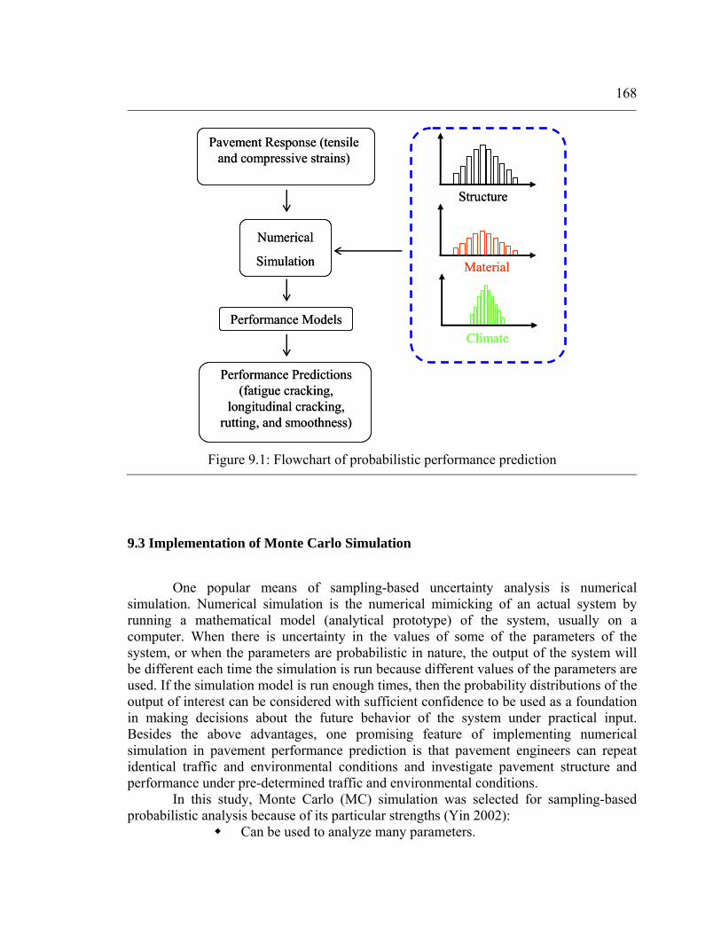
168

9.3 Implementation of Monte Carlo Simulation

One popular means of sampling-based uncertainty analysis is numerical simulation. Numerical simulation is the numerical mimicking of an actual system by running a mathematical model (analytical prototype) of the system, usually on a computer. When there is uncertainty in the values of some of the parameters of the system, or when the parameters are probabilistic in nature, the output of the system will be different each time the simulation is run because different values of the parameters are used. If the simulation model is run enough times, then the probability distributions of the output of interest can be considered with sufficient confidence to be used as a foundation in making decisions about the future behavior of the system under practical input. Besides the above advantages, one promising feature of implementing numerical simulation in pavement performance prediction is that pavement engineers can repeat identical traffic and environmental conditions and investigate pavement structure and performance under pre-determined traffic and environmental conditions.

In this study, Monte Carlo (MC) simulation was selected for sampling-based probabilistic analysis because of its particular strengths (Yin 2002):

Can be used to analyze many parameters.

Material

Climate

Structure

Performance Models

Pavement Response (tensile and compressive strains)

Numerical

Simulation

Performance Predictions (fatigue cracking,

longitudinal cracking, rutting, and smoothness)

Material

Climate

Structure

Performance Models

Pavement Response (tensile and compressive strains)

Numerical

Simulation

Performance Predictions (fatigue cracking,

longitudinal cracking, rutting, and smoothness)

Figure 9.1: Flowchart of probabilistic performance prediction

169

Handles different ways of specifying parameter distribution. Allows for tracking the propagation of uncertainty and variability

through model components at any level. Allows precision to be increased easily by performing additional

iterations. Briefly, the Monte Carlo simulation consists of formulating a game of chance or a stochastic process that produces a random variable whose expected value is the solution of a certain problem. An approximation to the expected value is then obtained by means of sampling from the resulting distribution. As in almost all numerical processes, only an approximation to the correct answer is obtained. In this case, instead of the primary source of error being due to numerical round-off, the primary source of error is due to the restriction of only being able to take a finite sample. The power of MC simulation relies on the ability to generate random numbers and sample values from a particular probability distribution.

9.3.1 Random Number Generation

Random numbers are real numbers distributed on the interval [0, 1] whose probability density function (PDF) is f(x) = 1, for 0 < x < 1; f(x) = 0 elsewhere. However, truly random numbers are unpredictable in advance and must be produced by an appropriate physical process such as radioactive decay. In practice, pseudorandom numbers are generally used instead and are produced in the computer by one of several simple algorithms and thus are predictable because their sequence is exactly reproducible. The term pseudorandom number refers to numbers that behave as if they are uniform random numbers but were, in fact, generated in a completely deterministic manner. Pseudorandom numbers are considered to be good when they exhibit the following characteristics: (1) statistical uniformity, (2) statistical independence, (3) reproducibility, and (4) they can be generated quickly and economically. Characteristics (1) through (3) are essential for good generators, while characteristic (4) is a function of time and budget. In the following subsections, the prefix ‘pseudo’ will be omitted.

Although there are a number of different methods (Lehmer 1951, Tausworthe 1965, Knuth 1969, Kirkpatrick and Stoll 1981, and James 1990) for generating random numbers, almost all random number generators in use today work in the following way. There is a “seed,” s = (s1,….,sm), that consists of m 32-bit computer integers. There is a mapping, s’ = F(s), that produces a new seed from a given one and a mapping, ξ = G(s), that produces a number in the interval [0, 1] from a seed. The mappings, F and G, are usually given by some modular arithmetic. To use such a random number generator, an initial seed, s1, is specified, and then the sequence ξ k is produced by repeatedly using F and G: ξ k = G(sk), sk+1 = F(sk).

170

9.3.2 Sampling Strategy

Conventional random sampling strategy samples values uniformly from the integration region of a particular probability distribution to estimate the integral and its error. However, Monte Carlo simulation typically requires a large number of repetitions to ensure sufficient opportunity to sample low probability values. This is especially true when highly skewed distributions are used to describe the input variables. When the number of repetitions performed is low, clustering can occur. In this situation, sampled values are tightly clustered around high probability outcomes, and the low probability outcomes may not be adequately sampled. Clustering is particularly important when low probability outcomes can have an inordinately serious effect on results.

Latin Hypercube (LH) sampling is a stratified sampling technique in which the probability scale of the cumulative distribution curve is divided into an equal number of probability ranges. The number of ranges used is equal to the number of repetitions performed in the simulation. LH sampling is very popular for use with computationally demanding models because its efficient stratification properties allow for the extraction of a large amount of uncertainty and sensitivity information with a relatively small sample size (Iman et al. 1979, Iman et al. 1980, and Startzman and Wattenbarger 1985). This feature makes LH an excellent candidate sampling strategy for pavement performance prediction involving cumulative damage analysis. A graphic comparison between 5000 conventional random samples and 1000 LH samples is shown in Figure 9.2. It indicates that LH sampling provides a reasonable approximation (red bar) of the specified Weibull distribution (light green area) at a much smaller sample size. Consequently, LH sampling was used in this research.

LH sampling operates in the following manner to generate a sample of size nS from the distributions D1, D2,..., Dn associated with the elements of x = [x1, x2,..., xn]. The range of each xj is exhaustively divided into nS disjoint intervals of equal probability, and one value xij is randomly selected from each interval. The nS values for x1 are randomly paired without replacement with the nS value for x2 to produce nS pairs. These pairs are then randomly combined without replacement with the nS values for x3 to produce nS triples. This process is continued until a set of nS nX-triples xi = [xi1, xi2, ., xi,n], i = 1, 2,..., nS, is obtained, with this set constituting the LH sample.

171

9.3.3 Optimum Number of Simulations

One major concern that may arise associated with the implementation of Monte Carlo simulation is the number of simulations. Of course, every simulation is different because each set of random numbers is different. The optimum number of simulations varies from problem to problem and depends on the required accuracy and acceptable computational time. Figure 9.3 gives an example of how the value of resilient modulus of Warren subgrade varies with different numbers of simulations. It is demonstrated that when the number of simulations is small (e.g., 500 simulations), the values of resilient modulus may fluctuate significantly. As the number of simulations increases (e.g., 5000 simulations), the simulated values of resilient moduli will converge to the specified lognormal distribution.

When more than one analysis parameter and/or probability distribution is involved in the simulation, such as performance prediction models, it is more difficult to determine the number of simulations from the visual inspection. The computed quantity obtained from an MC simulation is a sample average. Thus, its standard deviation is the standard deviation of the sample divided by the square root of the sample size (number of simulations). Although this is a point from the most elementary principles of statistics, it is worthwhile to distinguish between the standard deviation of a sample and the standard deviation of the sample mean. The latter is the former divided by the square root of the sample size. Hence, the sample mean is much less volatile than the sample values, themselves. Consequently, the error reduces at the rate of 1 over the square root of the sample size. This means that the sample accuracy increases as the sample size increases. The standard deviation of the sample is σ, and the number of simulations is n1. Since the outcome is a sample mean, the standard deviation of the estimate of the computed

(a) Conventional Random Sampling (b) Latin Hypercube Sampling

Figure 9.2: Simulated resilient modulus of Blair subbase (light green area – Weibull distribution, red area – random samples)

172

quantity is σ/ 1n . If the number of simulations is increased to n2, the standard deviation

of the estimate of the computed quantity will be σ/ 2n . Therefore, to achieve a 50 percent reduction in error (i.e., a 50 percent increase in accuracy), the number of simulations has to be quadrupled. The standard error reduces only at the rate of the square root of the sample size, not at the rate of the sample size itself. In this study, the antithetic variate method was adopted because it achieves greater accuracy with only a minimum increase in computational time (Hammersley and Handscomb 1964).

The following example demonstrates how the optimum number of simulations was determined. As shown in Table 9.1, one vehicle record was randomly selected from the traffic data collected from Warren. Corresponding pavement temperatures and layer stiffnesses were then obtained as described in Chapter 4. With the analytical strain prediction method developed in Chapter 6 and PDF determined in Chapter 8, the number of load repetitions of fatigue cracking was calculated using Equations 2.2 to 2.4. The accuracy and computational times of 100, 400, 1600, 6400, and 25,600 simulations were evaluated. As shown in Figure 9.4a, the standard error of the mean dramatically decreases as the number of simulations increases. This decreasing trend becomes weak after 6400 simulations. Figure 9.4b suggests that the computational time at 25,600 simulations is substantially larger than that at 6400 simulations. As a result, 5000 was selected as the

(a) 500 simulations (b) 1000 simulations

(c) 5000 simulations (d) 10000 simulations

Figure 9.3: Simulated resilient modulus of Warren subgrade

173

optimum number of simulations for future analysis because of its acceptable accuracy and computational time.

9.4 Evaluation of Performance Predictions

Pavements’ structural and function performances are typically evaluated through fundamental distresses in the pavement, such as cracks, rut depths, and smoothness. In this thesis research, distresses were predicted at weekly intervals using empirical performance models presented in Chapter 2. For each SISSI site, performance was also predicted using a deterministic approach in which no variability but, rather, the mean value of each site-specific parameter was considered. For the probabilistic approach, one performance prediction was randomly chosen from 5000 MC simulations of each vehicle pass for demonstration purposes. Both deterministic and probabilistic predictions are plotted in Figure 9.5 and Figure 9.6 for Warren and Blair sites, respectively. Complete prediction results are given in Appendix F. In general, for both the Warren and Blair sites,

Table 9.1: Summary of traffic data (10:24:38 p.m., 06/30/2003)

Vehicle Class Vehicle Speed, kph Axle Weight, kg Axle Spacing, m 1 5630 - - 2 8853 2-1 3.5 3 8172 3-2 1.3 4 9307 4-3 7.0

9 73

5 8808 5-4 2.7

0.0

1.0

2.0

3.0

4.0

5.0

6.0

7.0

0 6400 12800 19200 25600

Number of Simulations

Stan

dard

Err

or, E

6

0.0

1.0

2.0

3.0

4.0

5.0

6.0

0 6400 12800 19200 25600Number of Simulations

Com

puta

tiona

l Tim

e, se

c

(a) Standard Error of the Mean (b) Computational Time

Figure 9.4: Determination of optimum number of simulations

174

probabilistic and deterministic predictions show similar seasonal and yearly distress development. For instance, more distresses developed during hot seasons than in cold seasons. In other words, more damage was accumulated at high temperatures. Excessive rutting occurred in unbound layers at Blair during the first few weeks after the section was opened to traffic. This phenomenon may have resulted from a combined effect of the initial traffic compaction and the low resilient moduli in the summer. However, the deterministic approach predicts a sharp increase in all kinds of distresses close to the end of analysis period. There is also a considerable divergence between probabilistic and deterministic prediction of alligator cracking and smoothness for Blair.

0.0

1.0

2.0

3.0

4.0

5.0

0 30 60 90 120 150Pavement Age, week

Fatig

ue C

rack

ing,

%

ProbabilisticDeterministic

0.0

30.0

60.0

90.0

120.0


Lon

gitu

dina

l Cra

ckin

g, m

/km Probabilistic

Deterministic

(a) Alligator Cracking (b) Longitudinal Cracking

0.0

3.0

6.0

9.0

12.0


Rut

Dep

th, m

m


0.0

1.0

2.0

3.0

4.0


Rut

Dep

th, m

m


(c) AC Rutting (d) Unbound Rutting

0.0

3.0

6.0

9.0

12.0

15.0


Rut

Dep

th, m

m


0.600

0.800

1.000

1.200

1.400


IRI,

m/k

m


(e) Total Rutting (f) Smoothness

Figure 9.5: Probabilistic vs. deterministic performance predictions for Warren

(06/2003 – 05/2006)

175

Performance predictions were further evaluated by comparing them to field conditions. For the SISSI project, field conditions were obtained from manual distress surveys, transverse profiling, and longitudinal profiling. Performance predictions and available field condition data are summarized in Table 9.2 and Table 9.3 for Warren and Blair, respectively. Graphic comparisons are shown in Figure 9.7 and Figure 9.8. Several observations can be made through careful inspection of these figures:

For all kinds of distresses, both probabilistic and deterministic predictions are usually higher than field values. The discrepancy is

1.5

1.8

2.0

2.3

2.5

0 20 40 60 80 100 120Pavement Age, week

Fatig

ue C

rack

ing,

%


0.0

30.0

60.0

90.0


Lon

gitu

dina

l Cra

ckin

g, m

/km Probabilistic

Deterministic


0.0

1.0

2.0

3.0

4.0

5.0


Rut

Dep

th, m

m


0.0

1.0

2.0

3.0

4.0

5.0


Rut

Dep

th, m

m


(c) AC Rutting (d) Unbound Rutting

0.0

2.0

4.0

6.0

8.0

10.0


Rut

Dep

th, m

m


1.200

1.400

1.600

1.800

2.000

2.200


IRI,

m/k

m


(e) Total Rutting (f) Smoothness

Figure 9.6: Probabilistic vs. deterministic performance predictions for Blair

(07/2004 – 12/2006)

176

perhaps due to the national calibration coefficients in the empirical performance models.

A closer agreement between predictions and field conditions was observed for rutting and smoothness.

Between two survey dates, a significant increase in rut depth was captured by predictions, while no such increase was observed at Warren. Similar divergence was observed in longitudinal cracking at Blair. These differences may arise from the measurement error of manual distress survey and from transverse profiling.

For both the Warren and Blair sites, the probabilistic approach does not show much superiority over the deterministic approach for short-term performance prediction.

Table 9.2: Comparison of performance predictions and field conditions for Warren

Distress Mar-04 Dec-04 Feb-05 Jun-05 Probabilistic Prediction 1.4 2.6 2.6 3.5 Deterministic Prediction 1.4 2.6 2.8 3.4 Alligator

Cracking, % Field Condition - 0.2 - 2.3 Probabilistic Prediction 52.5 73.0 78.4 92.5 Deterministic Prediction 52.8 74.0 76.4 89.4 Longitudinal

Cracking, m/km Field Condition - 0.0 - 67.7 Probabilistic Prediction 6.6 9.4 9.4 10.3 Deterministic Prediction 6.8 9.2 9.6 10.3 Rut Depth, mm Field Condition 7.4 - 7.3 - Probabilistic Prediction 0.760 0.870 0.894 1.000 Deterministic Prediction 0.777 0.883 0.903 0.965 IRI, m/km Field Condition - 0.773 - 0.868

177

0.0

1.0

2.0

3.0

4.0

Mar-04 Dec-04 Feb-05 Jun-05

Fatig

ue C

rack

ing,

%Field ConditionProbabilistic PredictionDeterministic Prediction

0

30

60

90

120


Lon

gitu

dina

l Cra

ckin

g, m

/km Field Condition

Probabilistic PredictionDeterministic Prediction


0.0

5.0

10.0

15.0


Rut

Dep

th, m

m

Field ConditionProbabilistic PredictionDeterministic Prediction

0.000

0.300

0.600

0.900

1.200

1.500


IRI,

m/k

m

Field Condition

Probabilistic Prediction

Deterministic Prediction

(c) Rutting (d) Smoothness

Figure 9.7: Comparison of performance predictions and field conditions for Warren

178

Table 9.3: Comparison of performance predictions and field conditions for Blair

Distress Sep-04 Dec-05 Probabilistic Prediction 1.9 2.2 Deterministic Prediction 1.9 2.2 Alligator

Cracking, % Field Condition 0.0 1.4 Probabilistic Prediction 10.0 30.0 Deterministic Prediction 9.3 30.1 Longitudinal

Cracking, m/km Field Condition 0.0 0.0 Probabilistic Prediction 2.9 5.9 Deterministic Prediction 2.8 6.0 Rut Depth, mm Field Condition 2.7 3.9 Probabilistic Prediction 1.343 1.658 Deterministic Prediction 1.338 1.704 IRI, m/km Field Condition 1.444 1.397

179

9.5 Summary

This chapter presented a probabilistic approach in conjunction with the instrumentation data to predict pavement performance. The optimum number of Monte Carlo simulations was determined using the antithetic variate method such that the simulation accuracy and computational time can be improved to a great extent. Predicted pavement performance was evaluated using available field condition data for both Blair and Warren. Overall, both probabilistic and deterministic approaches provide reasonable short-term performance predictions. Thermal cracking was not considered in this study; consequently, the contribution of fatigue cracking, longitudinal cracking, and rutting to IRI may possibly be overestimated. The discrepancy observed between the predictions and field conditions is perhaps due to the national calibration coefficients in the empirical performance models. It is believed that with the availability of large amounts of field condition data, the MEPDG models could be more accurately calibrated locally. Consequently, the proposed probabilistic methodology can evaluate performance more efficiently.

0.0

1.0

2.0

3.0

4.0

Sep-04 Dec-05

Fatig

ue C

rack

ing,

%Field Condition



0.0

10.0

20.0

30.0

40.0

Sep-04 Dec-05

Lon

gitu

dina

l Cra

ckin

g, m

/km Field Condition

Probabilistic PredictionDeterministic Prediction


0.0

2.0

4.0

6.0

8.0

Sep-04 Dec-05

Rut

Dep

th, m

m

Field Condition



0.000

0.500

1.000

1.500

2.000

2.500

Sep-04 Dec-05

Rut

Dep

th, m

m

Field Condition



(c) Rutting (d) Smoothness

Figure 9.8: Comparison of performance predictions and field conditions for Blair

Chapter 10

Summary, Conclusions, and Recommendations

An accurate performance prediction is an involved and complex mission owing to a wide array of controlled and uncontrolled variables affecting the material properties, climate conditions, traffic loads, and subsequent structural response of the pavement section. Over the years, researchers have expended considerable effort toward arriving at a better understanding of pavement response and distress development in pavement structures. More recently, instrumentation has become a key implement in directly quantifying pavement response under diverse environmental and traffic conditions. This thesis research has been aimed at developing a methodology for predicting performance of flexible pavements with the use of instrumentation data. Detailed summary, conclusions, and recommendations are presented in the following sections.

10.1 Summary

In this research, a hybrid methodology incorporating both empirical performance models and mechanistic appraisal of pavement response was developed. This methodology can be generalized in an “if – then” flow of logic, as shown in Figure 10.1. Questions such as the following are asked in order to try to narrow down the viable prediction alternatives:

Is the amount of instrumentation data enough for an analytical response prediction?

Is it practicable to perform sophisticated FE modeling with computational resources on hand?

Is a probabilistic approach favored? Is performance model calibration preferred?

For example, in this research, simulated pavement responses from 3-D FEA were combined with field measurements to establish a “reasonably large” response database because the SISSI response data was not complete. Another flexibility of the developed methodology would be implementing probabilistic features in performance predictions. This thesis has demonstrated how to identify, quantify, and simulate the variabilities associated with design parameters through dense statistical analysis. Consequently, the effects of variabilities on performance predictions can be rationally assessed.

While the developed methodology is able to predict performance of the two research pavement sections using the M-E approach, it is also possible that the results from this research can be applied in a much broader manner, beyond the proposed research scope, such as in performance model calibration. Therefore, this methodology

181

should be considered a dynamic product, subject to change as dictated by the update/findings of the ongoing instrumentation projects and the state of practice in pavement design.

Evaluating Instrumentation Data

Is data complete?

YesAre computational resources sufficient?

No

Yes

No

LEA

FEA

Selecting Performance Models

Probabilistic Analysis

Yes

No

Performance Model Calibration?

Probabilistic Approach?

No

Yes

Field Condition

Predicting Performance

Evaluating Instrumentation Data

Is data complete?

YesAre computational resources sufficient?

No

Yes

No

LEA

FEA

Selecting Performance Models

Probabilistic Analysis

Yes

No

Performance Model Calibration?

Probabilistic Approach?

No

Yes

Field Condition

Predicting Performance

Figure 10.1: General layout of developed methodology

182

10.2 Findings and Conclusions

10.2.1 Principal Findings

The following principal findings may be drawn from this dissertation: 3-D finite element modeling is capable of simulating pavement

responses in the field. Pavement responses can be analytically estimated based on pavement

temperatures and vehicle speeds. Probabilistic performance predictions are in reasonable agreement

with field observations if variability and Monte Carlo simulation techniques are considered.

Probabilistic approach does not show much superiority over the deterministic approach for short-term performance prediction from measured and FE-simulated responses.

10.2.2 Conclusions

The following conclusions may be drawn from this dissertation: Instrumentation data can be effectively used to predict flexible

pavement performance. It is feasible to include probabilistic features in mechanistic-empirical

performance predictions.

10.3 Recommendations

The following recommendations are made for future research: The nonlinear behavior of granular materials and non-uniformity of

contact pressure should be considered in improving the accuracy of the FE-simulated pavement response.

Additional field response data are required to validate the analytical procedure for the response estimation because the procedure was developed using response data collected within a relatively narrow range of pavement temperatures and vehicle speeds.

Because of limited construction data of layer thickness, air voids, and effective binder content, normal distributions were assumed in the Monte Carlo simulation. Characterizing their probability distributions calls for more construction data.

183

More field condition data are needed so that the MEPDG performance models can be calibrated locally. Therefore, the proposed probabilistic methodology can evaluate performance more efficiently.

Bibliography

ABAQUS/Standard User’s Manual (2002) Finite Element Computer Program. Hibbitt, Karlsson and Sorenson, Inc., Pawtucket, RI, USA, Version 6.3.

Ahmed, Z., Marukic, I., Zaghloul, S., and Vitillo, N. (2005) “Validation of Enhanced Integrated Climatic Model Predictions Using New Jersey Seasonal Monitoring Data.” Paper presented at 84th Annual Meeting, Transportation Research Board, Washington D.C.

Al-Qadi, I. L., Loulizi, A., Elseifi, M., and Lahouar, S. (2004) "The Virginia Smart Road : The Impact of Pavement Instrumentation on Understanding Pavement Performance." The Journal of Association of Asphalt Paving Technologists Vol. 83.

Anderson, D. A. and LeBoon, J. (2002) Design and Construction of Loading Vehicle. Internal Report, The Pennsylvania State University, University Park, PA.

Anderson, D.A., Solaimanian, M., Hunter, D. and Soltani, A. (2003) Superpave Validation Studies : SISSI Instrumentation, Operating Instructions and Baseline Measurements. Final Report, Pennsylvania Transportation Institute, University Park, PA.

Anderson, T. W. and Darling, D. A. (1952). "Asymptotic Theory of Certain "Goodness-of-fit" Criteria Based on Stochastic Processes." Annals of Mathematical Statistics 23.

Applied Research Associates, Inc. and Arizona State University (2006) Technical Assistance to NCHRP and NCHRP Project 1-40: Versions 0.9 and 1.0 of the M-E Pavement Design Software, NCHRP Project 1-40. Transportation Research Board, National Research Council, Washington, DC.

Baker, H. B., Buth, M. R., and Van Deusen, D. A. (1994) Minnesota Road Research Project: Load Response Instrumentation Installation and Testing Procedures. Final Report, 1992-94, Report No. MN/PR-94/01, Minnesota Dept. of Transportation, Maplewood, MN.

Bathe, K. J. (1982) Finite Element Procedures in Engineering Analysis, Prentice-Hall, NJ.

Birgisson, B., Ovik, J., and Newcomb, D. (2000) “Analytical Predictions of Seasonal Variations in Flexible Pavements at the Mn/Road Site.” Transportation Research Record No. 1730, National Research Council, Washington, D.C.

Bao, W. (2000) Calibration of Flexible Pavement Structural Model Using MnRoad Field Data. MS Thesis, Department of Civil Engineering, University of Minnesota, Minneapolis, MN.

185

Castillo, E. (1988) Extreme Value Theory in Engineering. Academic Press, Inc. San Diego, CA.

Carvalho, R.L. and Schwartz, C.W. (2006) “Comparisons of Flexible Pavement Designs: AASHTO Empirical versus NCHRP Project 1-37A Mechanistic-Empirical.” Transportation Research Record No.1947, Transportation Research Board, Washington, D.C.

Chakravarti, I.M., Laha, R.C., and Roy, J. (1967) Handbook of Methods of Applied Statistics, Volume I. John Wiley and Sons.

Chambers, J.M., Cleveland, W.S., Kleiner, B., and Tukey, P.A. (1983) Graphical Methods for Data Analysis. Wadsworth International Group, Belmont, CA.

Chatti, K., Kim, H.B., Yun, K.K., Mahoney, J.P. and Monismith, C.L. (1996) “Field Investigation into Effects of Vehicle Speed and Tire Pressure on Asphalt Concrete Pavement Strains.” Transportation Research Record No. 1539, Transportation Research Board, Washington, D.C.

Chehab, G. R. (2002) Characterization of Asphalt Concrete in Tension Using a ViscoElastoPlastic Model. Ph.D. Dissertation, North Carolina State University, NC.

Chen, D.H., Zaman, M., Laguros, J., and Soltani, A. (1995) “Assessment of Computer Programs for Analysis of Flexible Pavement Structures.” Transportation Research Record 1539, Transportation Research Board, Washington, DC.

Chernoff, H and Lehmann, E.L. (1954) “The Use of Maximum Likelihood Estimates in χ2 Tests for Goodness-of-fit.” The Annals of Mathematical Statistics.

Cho, Y.H., McCullough, B.F., and Weissmann, J. (1996) “Considerations on Finite-Element Method Application in Pavement Structural Analysis.” Transportation Research Record 1539, Transportation Research Board, Washington, DC.

Darter, M.I. and Hudson, W.R. (1973) Probabilistic Design Concepts Applied to Flexible Pavement System Design. Report No. 123-18, Center for Highway Research, University of Texas at Austin, TX.

De Beer, M. (1996) Measurement of Tyre/Pavement Interface Stresses under Moving Wheel Loads. Int. J. of Vehicle Design. Vol. 3.

De Jong, D.L., Peatz, M.G.F., and Korswagen, A.R. (1973) Computer Program Bisar Layered System Under Normal and Tangential Loads. Konin Klijke Shell-Laboratorium, Amsterdam, Netherlands.

El-Basyouny, M.M. and Witczak, M.W. (2005) “Calibration of alligator fatigue cracking model for 2002 Design Guide.” Transportation Research Record No.1919, Transportation Research Board, Washington, D.C.

El-Basyouny, M.M., Witczak, M.W., El-Badawy, S., Timm, D., Dongre, R., Heitzman, M., and Dunning, R. (2005a) “Verification for the Calibrated Permanent

186

Deformation Models for the 2002 Design Guide.” Journal of the Association of Asphalt Paving Technologists, Vol. 74.

El-Basyouny, M.M., Witczak, M.W., Tam, K., Monismith, C., Harman, T., and Brown, S. (2005b) “Verification of the Calibrated Fatigue Cracking Models for the 2002 Design Guide.” Journal of the Association of Asphalt Paving Technologists, Vol. 74.

Elseifi, M.A., Al-Qadi, I.L., and Yoo, P.J. (2006) Viscoelastic Modeling and Field Validation of Flexible Pavements. Journal of Engineering Mechanics, Vol. 132, No. 2.

ERES Consultants Division. (2004) Guide for Mechanistic-Empirical Design of New and Rehabilitated Pavement Structures. Final Report NCHRP 1-37A, Champaign, IL.

Federal Highway Administration. (2001) Guide to LTPP Traffic Data Collection and Processing. FHWA, Washington, DC.

Fanous, F., Coree, B., and Wood, D. (1999) Response of Iowa Pavements to Heavy Agricultural Loads. Department of Civil and Construction Engineering, Iowa State University, IA.

Freeman, T., Uzan, J., Zollinger, D., and Park, E. (2005) Sensitivity Analysis of and Strategic Plan Development for the Implementation of the M-E Design Guide in TXDOT Operations. Report No. 0-4714-1, Texas Transportation Institute, College Station, TX.

Galal, K. and Chehab, G.R. (2005) “Implementation of the 2002 M-E Design Procedure Using a HMA Rehabilitated Pavement Section in Indiana.” Transportation Research Record No.1919, Transportation Research Board, Washington, D.C.

Hammersley, J. M. and Handscomb, D. C. (1964) Monte Carlo Methods. Chapman and Hall, London & New York.

Heydinger, A.G. (2003) Monitoring Seasonal Instrumentation and Modeling Climatic Effects on Pavements at the Ohio/SHRP Test Road. Final Report, Report No FHWA/OH-2003/018, Department of Civil Engineering, The University of Toledo, Toledo, OH.

Hjelmsted, K.D., Kim, J., and Zuo, Q. (1997) “Finite Element Procedures for Three Dimensional Pavement Analysis.” Aircraft/Pavement Technology: In the Midst of Chang, Proceedings, ASCE Airfield Pavement Conference, Seattle, WA.

Huang, Y. (1993) Pavement Analysis and Design. Prentice Hall, NJ.

Huhtala, M. and Pihlajamaki, J. (1992). “Strain and Stress Measurements in Pavements.” Proceedings, Road and Airport Pavement Response Monitoring Systems, ASCE.

Hull, J. (2005) Properties of Lognormal Distribution, in Options, Futures, and Other Derivatives 6E.

187

Iman, R. L. (1992) “Uncertainty and Sensitivity Analysis for Computer Modeling Applications.” Presented at Reliability Technology - 1992, The Winter Annual Meeting of the American Society of Mechanical Engineers, Anaheim, CA.

Iman, R.L., Conover, W.J., and Beckman, R.J. (1979) “A Comparison of Three Methods for Selecting Values of Input Variables in the Analysis of Output from a Computer Code.” Technometrics.

Iman, R.L., Davenport, J.M., and Zeigler, D.K. (1980) Latin Hypercube Sampling (A Program Users Guide). Technical Report SAND79-1473, Sandia Laboratories, Albuquerque, NM.

James, F. (1990) “A Review of Pseudorandom Number Generators.” Comput. Phys. Commun, Vol. 60.

Kim, S., Ceylan, H., and Heitzman, M. (2005) “Sensitivity Study of Design Input Parameters for Two Flexible Pavement Systems Using the Mechanistic-Empirical Pavement Design Guide.” Proceedings, the 2005 Mid-Continent Transportation Research Symposium, Ames, IA.

Kirkpatrick, S. and Stoll, E. P. (1981) “A Very Fast Shift-Register Sequence Random Number Generator.” J. Comput. Phys, Vol. 40.

Knuth, D. (1969) The Art of Computer Programming. Vol 2: Seminumerical Algorithms.

Kuo, M. C., Hall, K. T., and Darter, M. (1995) “Three-dimensional Finite Element Model for Analysis of Concrete Pavement Support.” Transportation Research Record No. 1505, Transportation Research Board, Washington, D.C.

Larson, G. and Dempsey, B. J. (1997) Enhanced Integrated Climatic Model, Version 2.0. Final Report, Contract DTFA MN/DOT 72114, Department of Civil Engineering, University of Illinois at Urbana-Champaign, Urbana, IL.

Law, A.M. and Kelton, W.D. (1991) Simulation Modeling and Analysis. McGraw-Hill, Inc. New York.

Lehmer, D.H. (1951) “Large-Scale Digital Computing Machinery.” Proceedings, 2nd Symp. Cambridge, MA.

Li, Y. and Metcalf, J.B. (2002) “Crack Initiation Model from Asphalt Slab Tests.” Journal of Materials in Civil Engineering, ASCE.

Liang, Robert Y., Rabab’ah, S., Al-Akhras, K. (2006) “Validation of Enhanced Integrated Climatic Model Prediction Over Different Drainable Base Materials.” presented at 85th Annual Meeting, Transportation Research Board, Washington D.C.

Luo, R. and Prozzi, J. (2005) Evaluation of the Joint Effect of Wheel Load and Tire Pressure on Pavement Performance. Center for Transportation Research, University of Texas at Austin, TX.

Loulizi, A., Al-Qadi, I. L., Lahouar, S., and Freeman, T.E. (2001) “Data Collection and Management of the Instrumented Smart Road Flexible Pavement Sections.”

188

Transportation Research Record No.1769, Transportation Research Board, Washington, DC.

Lukanen, Erland O., Stubstad, R., Briggs, R. (2000) Temperature Predictions and Adjustment Factors for Asphalt Pavements. Report FHWA-RD-98-085, Federal Highway Administration, McLean, VA.

Lytton, R.L., Pufahl, D.E., Michalak, C. H., Liang, H. S., and Dempsey, B. J. (1990) An Integrated Model of the Climatic Effects on Pavement. Texas Transportation Institute, Texas A&M University, Report No FHWA-RD-90-033, 1990, Federal Highway Administration, McLean, VA.

Lytton, L.R., Uzan, J., Fernando, E. G., Roque, R., Hiltunen, D., and Stoffels, S.M. (1993) Development and Validation of Performance Prediction Models and Specifications for Asphalt Binders and Paving Mixes. SHRP-A-357 Report. Strategic Highway Research Program, National Research Council, Washington, D.C.

Marshall, C., Meier, R., and Weilch M. (2001) “Seasonal Temperature Effects on Flexible Pavements in Tennessee.” Transportation Research Record No. 1764, Transportation Research Board, Washington, D.C.

Masad, S.A. and Little, D.N. (2004) Sensitivity Analysis of Flexible Pavement Response and AASHTO 2002 Design Guide for Properties of Unbound Layers. Report No. ICAR 504-1, International Center for Aggregates Research, Austin, TX.

Moreno, A.M. (2000) Load Equivalency Factors from the Structural Response of Flexible Pavements. MS Thesis, Department of Civil Engineering, University of Minnesota, MN.

Newcomb, D.E., Bu-bushait, A.A., Mahoney, J.P. and Sharma, J. (1983) State-of-the-Art on Pavement Overlay Design Procedures. Vol. 1. Report No. WA-RD 65.1, Washington State Department of Transportation, Olympia, WA.

Ongel, A. and Harvey, J. (2004) Analysis of 30 Years of Pavement Temperatures using the Enhanced Integrated Climate Model (EICM). Draft report prepared for the California Department of Transportation, Pavement Research Center, Institute of Transportation Studies, University of California, Berkeley, University of California, Davis, CA.

Pirabaroobn, S., Zaman, M., and Tarefder, R.A. (2003) “Evaluation of Rutting Potential in Asphalt Mixes Using Finite Element Modeling.” 2003 Annual Conference of the Transportation Association of Canada, St. John’s, Newfoundland and Labrador, USA.

Ridgeway, H.H. (1982) Pavement Subsurface Drainage Systems, Synthesis of Highway Practice 96. Transportation Research Board, Washington, D.C.

Sargand, S. M., Green, R., and Khoury, I. (1997) “Instrumentation Ohio Test Pavement.” Transportation Research Record No.1596, Transportation Research Board, Washington, DC.

189

Schapery, R. and Park, S. (1999) “Methods of Interconversion Between Linear Viscoelastic Material Functions. Part II – An Approximate Analytical Method.” International Journal of Solids and Structures, Vol. 36.

Schwartz, C. W., Gibson, N., and Schapery, R. A. (2002) “Time-Temperature Superposition for Asphalt Concrete at Large Compressive Strains.” Transportation Research Record No. 1789, Transportation Research Board, Washington, D.C.

Selezneva, Olga I., Jiang, Y. J., and Mladenovic, G. (2002) Evaluation and Analysis of LTPP Pavement Layer Thickness Data. Report No. FHWA-RD-03-041, Federal Highway Administration, VA.

Shoukry, S. (1998a) “3D Finite Element Modeling for Pavement Analysis and Design.” Proceedings, First National Symposium on 3D Finite Element Modeling for Pavement Analysis and Design, Charleston, WV.

Sebaaly, P. E. and Mamlouk, M. (1987) Prediction of Pavement Response to Actual Traffic Loading. Transportation Research Board, Washington, D.C.

Sebaaly, P. E., and Tabatabaee, N. (1991) “Field Evaluation of Strain Gauges in Asphalt Concrete Pavements.” Proceedings, Road and Airport Pavement Response Monitoring Systems, ASCE.

Siddharthan, Raj V., Krishnamenon, N., El-Mously, M., and Sebaaly, Peter E. (2002) “Investigation of Tire Contact Stress Distributions on Pavement Response.” J. Transp. Engrg., Vol. 128, Issue 2.

Solaimanian, M., Hunter, D., and Stoffels, S. M. (2006) Design and Construction Report for Superpave In-Situ Stress-Strain Instrumentation Sites, State Route 1001, Blair County, Pennsylvania. Final Report, Pennsylvania Transportation Institute, University Park, PA.

Solaimanian, M., Stoffels, S. M., Anderson, D. A., and Morian, D. (2006) Design and Construction Report for Superpave In-Situ Stress-Strain Instrumentation Sites, State Route 0006, Warren County, Pennsylvania. Final Report, Pennsylvania Transportation Institute, University Park, PA.

Solaimanian M., Hunter, D. A., Shah, J., and Stoffels, S. M. (2006) Characterization of Materials for Superpave In-Situ Stress/Strain Investigation. Final Report, Pennsylvania Transportation Institute, University Park, PA.

Solaimanian M., Stoffels, S. M., Hunter, D. A., Morian, D., and Sadavisam, S. (2006) Detailed Final Report for Superpave In-Situ Stress/Strain Investigation. Final Report, Pennsylvania Transportation Institute, University Park, PA.

Startzman, R.A. and Wattenbarger, R.A. (1985) “An Improved Computation Procedure for Risk Analysis Problems with Unusual Probability Functions.” Proceedings, SPE Hydrocarbon Economics and Evaluation Symposium, Dallas, TX.

Stoffels, S. M. and Solaimanian M. (2003) Performance, Traffic and Weather Data Collection and Reporting Manual for Superpave In-Situ Stress/Strain

190

Investigation. Final Report, Pennsylvania Transportation Institute, University Park, PA.

Stoffels, S. M., Solaimanian M., and Morian, D. (2006) Seasonal Variations for Superpave In-Situ Stress/Strain Investigation. Final Report, Pennsylvania Transportation Institute, University Park, PA.

Stoffels, S. M. and Solaimanian M. (2006) Pavement Condition for Superpave In-Situ Stress/Strain Investigation. Final Report, Pennsylvania Transportation Institute, University Park, PA.

Stoffels, S., Yin, H., Antle, C., Schwartz, C., and Lim, S. (2006). Integrating Condition Measurement Variability in Network Pavement Management. Final Report, Contract DTFH61-02-D-00137, Federal Highway Administration, U.S. Department of Transportation, Washington, D.C.

Tausworthe, R. C. (1965) “Random Numbers Generated by Linear Recurrence Modulo Two.” Math. Comput, 19.

Timm, D.H. and Newcomb, D.E. (2003) “Calibration of Flexible Pavement Performance Equations.” Transportation Research Record 1853, Transportation Research Board, Washington, D.C.

Timm, D. H., Priest, A. L., and McEwen, T. V. (2004) Design and Instrumentation of The Structural Pavement Experiment at The NCAT Test Track, NCAT Report 04-01. National Center for Asphalt Technology, Auburn University, Auburn, AL.

Timm, D.H., Bower, J.M., and Turochy, R.E. (2006) “Effect of Load Spectra on Mechanistic-Empirical Flexible Pavement Design.” Transportation Research Record No.1947, Transportation Research Board, Washington, D.C.

Titus-Glover, L., Mallela, J., Jiang, Y. J., Ayers, M. E., and Shami, H. I. (2001) Assessment of Selected LTPP Material Data Tables and Development of Representative Test Tables. Report No. FHWA-RD-02-001, Federal Highway Administration, VA.

The AASHTO Road Test (1962) Report 6 – Special Studies, HRB Spec. Report 61F.

Uddin, W. (1998) “Application of 3D Finite Element Dynamic Analysis for Pavement Evaluation.” Proceedings, First National Symposium on 3D Finite Element Modeling for Pavement Analysis and Design, Charleston, WV.

Von Quintus, H.L., Schwartz, C.W., McCuen, R.H., and Andrei, D. (2003) Experimental Plan for Calibration and Validation of Hot Mix Asphalt Performance Models for Mix and Structural Design. Final Report, NCHRP Project 9-30, Transportation Research Board, National Research Council, Washington, DC.

Weibull, W. (1951) "A Statistical Distribution Function of Wide Applicability." J. Appl. Mech.-Trans. ASME 18(3).

191

White, T. (1998) “Application of Finite Element Analysis to Pavement Problems.” Proceedings, First National Symposium on 3D Finite Element Modeling for Pavement Analysis and Design, Charleston, WV.

Wu, Z. and Hossain, M (2003) Pilot Instrumentation Of A Superpave Test Section At The Kansas Accelerated Testing Laboratory. Final Report, Report No KTRAN: KSU-98-2, Department of Civil Engineering, Kansas State University, Manhattan, KS.

Yin, H., Imad, A., and Ferregut, C. (2002) Optimizing Construction Quality Management of Pavements Using Mechanistic Performance Analysis. Report 0-4046-1, Center of Highway Materials Research, University of Texas at El Paso, El Paso, TX.

Yin, H. (2002) Optimizing Construction Quality Management of Pavements Using Mechanistic Performance Analysis. MS Thesis, University of Texas at El Paso, El Paso, TX.

Yin, H., Chehab, G., and Stoffels, S. (2006) “A Case Study: Assessing the Sensitivity of the Coefficient of Thermal Contraction of AC Mixtures on Thermal Crack Prediction.” ASCE Geotechnical Special Publication No.146.

Yin, H., Chehab, G., and Stoffels, S. (2006) “Sensitivity of Thermal Cracking Prediction to AC Mixture Properties Using the M-E Pavement Design Guide.” Presented at the 10th International Conference on Asphalt Pavements, Quebec, Canada.

Zaghloul, S. M., and White, T. D. (1993) “Use of a Three-dimensional, Dynamic Finite Element Program for Analysis of Flexible Pavement.” Transportation Research Record No. 1388, Transportation Research Board, Washington, D.C.

Zaghloul, S., Gucunski, N., Jackson, H., and Hadidi, R. (2006) Material Characterization and Seasonal Variation in Material Properties. Final Report, Report No FHWA NJ-2005-024, Center for Advanced Infrastructure and Transportation, Dept. of Civil & Environmental Engineering, Rutgers, the State University, Piscataway, NJ.

Zelen, M. and Severo, N.C. (1964). Probability Functions. Handbook of Mathematical Functions with Formulas, Graphs, and Mathematical Tables, Chapter 26. Milton Abramowitz and Irene A. Stegun. National Bureau of Standards.

Appendix A

Transducer Layout

12.5 mm ACC

19 mm ACC

200 mm 2A Subbase

Left WP

Right WP

P

P P

P

25 mm ACC

G

F

G

GG

4020

018

050

P P

CL1 m

S S

6

6 6

6

Plan

Vie

wTr

avel

Lan

ePr

ofile

Vie

w

6

6

M

Subgrade

F

M 5

PG

Sin

gle

Laye

r Def

lect

omet

erS

PAST

II L

ongi

tudi

nal

PAST

II T

rans

vers

eFr

ost D

epth

MD

DPr

essu

re C

ell

Geo

kon

3900

Stra

in G

age

CS

315

Moi

stur

e C

ell

Des

ign

Thic

knes

ses,

mm

County Location Section SISSI No. Segment Offset

Blair SR 1001 Southbound 8-1012 - -

S M

Figure A1: Layout of transducers at Warren

193

51

Wearing

Binder

Lev elling

Left WP

Right WP

Base

3814

051

CL1 m

Plan

Vie

wTr

avel

Lane

Prof

ile Vi

ew

FPA

ST II L

ongi

tudi

nal

PAST

II Tra

nsve

rse

Fros

t Dep

thF

Des

ign T

hick

ness

es, m

m

County Loca tion Section SISS I No. Segment Offset

4-2A01 420 788SR 0006 EastboundWarren

Figure A2: Layout of transducers at Warren

Appendix B

Validation Results of FE Models

Run# Load Configuration Location Season Axle Actual Speed,

kph Data Source Strain, E-6

1 B Wearing Spring 1 42 Measured 32.6

1 B Wearing Spring 1 42 Predicted 29.0







1 B Binder Spring 1 42 Measured 22.1

1 B Binder Spring 1 42 Predicted 19.8







1 B BCBC Spring 2 42 Measured 15.8

1 B BCBC Spring 2 42 Predicted 14.1





Table B1: Summary of measured and FE simulated horizontal strains for Blair

195

2 B Wearing Summer 1 61 Measured 22.8

2 B Wearing Summer 1 61 Predicted 20.0







2 B Binder Summer 1 61 Measured 12.7

2 B Binder Summer 1 61 Predicted 11.2







2 B BCBC Summer 1 61 Measured 13.3

2 B BCBC Summer 1 61 Predicted 11.8







3 F Wearing Summer 1 39 Measured 56.4

3 F Wearing Summer 1 39 Predicted 49.6






196


3 F Binder Summer 1 39 Measured 24.2

3 F Binder Summer 1 39 Predicted 21.4







3 F BCBC Summer 1 39 Measured 24.3

3 F BCBC Summer 1 39 Predicted 21.5







4 B Wearing Fall 1 35 Measured 18.4

4 B Wearing Fall 1 35 Predicted 16.3







4 B Binder Fall 1 35 Measured 6.9

4 B Binder Fall 1 35 Predicted 6.2





197



4 B BCBC Fall 1 35 Measured 4.8

4 B BCBC Fall 1 35 Predicted 4.3




























198
































199
































200














9 F Wearing Spring 1 14 Measured 28.9

9 F Wearing Spring 1 14 Predicted 25.7







9 F Binder Spring 1 14 Measured 18.3

9 F Binder Spring 1 14 Predicted 16.4







9 F BCBC Spring 1 14 Measured 8.1

9 F BCBC Spring 1 14 Predicted 7.3

201
































202
































203

























204

Run# Load Configuration Location Season Axle Actual

Speed, kph Data Source Vertical Stress, kPa

1 B Subbase Spring 1 42 Measured 12.9

1 B Subbase Spring 1 42 Predicted 14.7







2 B Subbase Summer 1 61 Measured 12.2

2 B Subbase Summer 1 61 Predicted 14.0







3 F Subbase Summer 1 39 Measured 17.4

3 F Subbase Summer 1 39 Predicted 19.9







4 B Subbase Fall 1 35 Measured 7.8

4 B Subbase Fall 1 35 Predicted 8.9



Table B2: Summary of measured and FE simulated vertical stresses for Blair

205













6 B Subgrade Spring 1 12 Measured 9.3

6 B Subgrade Spring 1 12 Predicted 10.6


















206






9 F Subbase Spring 1 14 Measured 10.7

9 F Subbase Spring 1 14 Predicted 12.2







9 F Subgrade Spring 1 14 Measured 4.6

9 F Subgrade Spring 1 14 Predicted 5.2

















207
































208






209

Run# Load Configuration Location Season Axle Actual

Speed, kph Data Source Strain, E-6





























Table B3: Summary of measured and FE simulated horizontal strains for Warren

210
































211
































212





























10 F Binder Fall 1 36 Measured 6.4

10 F Binder Fall 1 36 Predicted 5.9

10 F BCBC Fall 1 36 Measured 5.4

213

10 F BCBC Fall 1 36 Predicted 5.0































214
































215
































216
































217
































218
































219


















Appendix C

Response Database

Analysis Location Pavement Temperature, oC Vehicle Speed, kph Tensile Strain, E-6

Bottom of Wearing 13 12 41.0









Bottom of Binder 15 12 19.8









Bottom of BCBC 12 12 18.9





Table C1: Tensile strains for Blair

221





222

Analysis Location Pavement Temperature, oC Vehicle Speed, kph Compressive Strain, E-6

Top of Binder 13 12 87.2









Top of BCBC 15 12 55.3



Top of BCBC 33 38 168.4

Top of BCBC 33 54 154.0

Top of BCBC 33 65 139.1




Top of Subbase 12 12 60.9









Top of Subgrade 10 12 43.9

Table C2: Compressive strains for Blair

223









224

Analysis Location Pavement Temperature, oC Vehicle Speed, kph Tensile Strain, E-6




























Bottom of Leveling 5 34 3.5

Table C3: Tensile strains for Warren

225









226

Analysis Location Pavement Temperature, oC Vehicle Speed, kph Compressive Strain, E-6













Top of BCBC 27 36 158.1

Top of BCBC 27 68 112.1





Top of Leveling 5 34 26.1









Top of Fractured PCC 5 34 10.9

Table C4: Compressive strains for Warren

227


















Appendix D

MEPDG Input Summary for Warren

229

Limit Reliability 45 172 90 1000 90 25 90 1000 90 0.25 90 0.75 90

422 2 50 90.5 58

Class 4 Class 5 Class 6 Class 7 Class 8 Class 9 Class 10 Class 11 Class 12 Class 13

1.12 0.48 0.74 0.36 0.93 0.88 0.46 0.34 1.41 0.351.04 0.54 0.88 0.68 0.90 0.91 0.62 0.46 1.76 0.350.87 0.90 0.82 0.55 0.93 0.95 0.85 0.69 0.00 0.841.18 1.04 0.84 0.91 1.09 1.03 0.75 1.40 0.00 1.331.27 1.25 1.13 1.13 0.98 1.07 0.91 1.01 0.00 1.400.83 1.29 1.15 1.52 1.04 1.09 1.01 1.84 0.00 0.980.63 1.18 1.16 1.11 1.07 1.06 0.95 0.71 0.00 1.330.82 1.19 1.31 1.07 1.12 1.11 1.01 0.47 7.06 1.281.38 1.14 1.36 1.21 1.08 1.03 1.55 1.45 0.00 0.981.14 1.16 1.08 1.59 1.02 1.08 1.48 1.45 1.76 1.610.89 0.94 0.82 1.01 0.94 0.94 1.08 0.53 0.00 0.000.84 0.89 0.71 0.86 0.91 0.83 1.32 1.65 0.00 1.54

Midnight 1.3% Noon 6.5% 1.7% 1:00 am 1.5% 1:00 pm 6.1% 22.5% 2:00 am 2.0% 2:00 pm 6.0% 12.5% 3:00 am 2.9% 3:00 pm 5.4% 6.7% 4:00 am 3.6% 4:00 pm 4.6% 2.7% 5:00 am 4.0% 5:00 pm 3.5% 52.9% 6:00 am 5.4% 6:00 pm 2.9% 0.9% 7:00 am 6.7% 7:00 pm 2.4% 0.1% 8:00 am 7.2% 8:00 pm 2.1% 0.0% 9:00 am 7.1% 9:00 pm 1.8% 0.0% 10:00 am 7.0% 10:00 pm 1.7% 11:00 am 6.9% 11:00 pm 1.4%

Class 13

Class 9Class 10Class 11Class 12


(Level 1, Site Specific Distribution ) by period beginning:AADTT distribution by vehicle classClass 4

NovemberDecember

Vehicle Class Distribution Hourly truck traffic distribution

JulyAugustSeptemberOctober

MarchAprilMayJune

Vehicle ClassMonth

JanuaryFebruary

Percent of trucks in design lane (%):Operational speed (mph):

Traffic -- Volume Adjustment FactorsMonthly Adjustment Factors (Level 1, Site Specific - MAF)

TrafficInitial two-way aadtt:Number of lanes in design direction:Percent of trucks in design direction (%):

Traffic direction: East bound

Project ID: SR 0006Section ID: Segment 420

Permanent Deformation (AC Only) (in):Permanent Deformation (Total Pavement) (in):

Location: Starbrick, Warren County, PA

Terminal IRI (in/mi)AC Surface Down Cracking (Long. Cracking) (ft/mile):AC Bottom Up Cracking (Alligator Cracking) (%):AC Thermal Fracture (Transverse Cracking) (ft/mi):

Performance CriteriaInitial IRI (in/mi)

October, 2001Type of design Flexible

General InformationDesign Life 20 yearsPavement overlay construction: September, 2001Traffic open:

230

4.0% 4.0% 4.0% 4.0% 4.0% 4.0% 4.0% 4.0% 4.0% 4.0%

18 10 12

1.85 0.15 0.00 0.00 2.00 0.01 0.00 0.00 1.00 1.00 0.00 0.00 1.00 0.00 1.00 0.00 2.31 0.69 0.00 0.00 1.22 1.89 0.00 0.00 1.02 1.00 0.99 0.00 5.00 0.00 0.00 0.00 4.00 1.00 0.00 0.00 1.21 0.88 0.94 0.33

8.5 12 120 50.6 54.1 48.1

41.51 -79.18 1259 10

Latitude (degrees.minutes)Longitude (degrees.minutes)Elevation (ft)Depth of water table (ft)

Quad axle(psi):

Climateicm file: C:\DG2002\Projects\Warren\Warren.icm

Average Axle Spacing

Tandem axle(psi):Tridem axle(psi):

Average axle width (edge-to-edge)outside dimensions,ft):Dual tire spacing (in):

Axle ConfigurationTire Pressure (psi) :

Class 11Class 12Class 13

Axle Configuration


QuadAxle

Class 4Class 5Class 6

VehicleClass

SingleAxle

TandemAxle

TridemAxle

Mean wheel location (inches from thelane marking):Traffic wander standard deviation (in):Design lane width (ft):

Number of Axles per Truck

Traffic -- Axle Load Distribution FactorsLevel 1: Site Specific

Traffic -- General Traffic Inputs

Class 12 No GrowthClass 13 No Growth





Traffic Growth Factor

VehicleClass

GrowthRate

GrowthFunction

231

0.5 1 5 10 25 1319287 1540373 1868956 2016895 2251469 794594 940212 1217930 1343920 1531308 227071 293837 487569 588660 740563 32914 60302 123379 165778 248740 15264 23773 59008 83291 126335

Total unit weight (pcf): 142

Poisson's ratio: 0.35 (user entered)

Volumetric Properties as BuiltEffective binder content (%): 9.3Air voids (%): 5.7

General PropertiesGeneralReference temperature (F°): 77

Material type: Asphalt concreteLayer thickness (in): 2.5

177.8 370 89

Layer 2 -- Asphalt concrete

158 1371 86167 699 88

136.4 6241 82147.2 2861 84

114.8 33601 76125.6 14109 79

Temperature°F

Angular frequency = 10 rad/secG*, psi Delta (°)

127.4

Asphalt BinderOption: Superpave binder test data

39.25077104

Number of frequencies: 5

Temperature°F

Mixture E* (psi)

Heat capacity asphalt (BTU/lb-F°): 0.23

Asphalt MixNumber of temperatures: 5


Thermal PropertiesThermal conductivity asphalt (BTU/hr-ft-F°): 0.67

Air voids (%): 6.4Total unit weight (pcf): 137

Reference temperature (F°): 77

Volumetric Properties as BuiltEffective binder content (%): 12.7

Layer thickness (in): 1.5

General PropertiesGeneral

Structure--Design Features

Structure--LayersLayer 1 -- Asphalt concrete

Material type: Asphalt concrete

232

0.1 0.5 1 5 10 25 1289966 1465848 1691053 1944956 2086126 2290194 910305 1138609 1325340 1610934 1740211 1947905 289350 472997 575698 831260 958603 1151165 58837 114904 160528 304144 385075 523925 20870 55428 79864 166782 219385 304343

0.1 0.5 1 5 10 25 1446703 1669201 1868125 2171167 2299912 2462257 1003516 1275583 1483011 1801804 1946551 2141386 276152 507763 608989 902473 1049831 1259459 48394 101613 147827 301388 388749 532288 14974 45682 69019 157194 212811 304654

77104

127.4

Temperature°F

Mixture E* (psi)

39.250

Asphalt MixNumber of temperatures: 5Number of frequencies: 6

Thermal PropertiesThermal conductivity asphalt (BTU/hr-ft-F°): 0.67Heat capacity asphalt (BTU/lb-F°): 0.23

Total unit weight (pcf): 147.5





177.8 425 88


156.2 1646 86167 815 87

136.4 7754 81147.2 3481 83

114.8 42069 75125.6 17537 78

Option: Superpave binder test data

Temperature°F


77104

127.4

Asphalt Binder

Temperature°F

Mixture E* (psi)

39.250



233

0.1 0.5 1 5 10 25 1289966 1465848 1691053 1944956 2086126 2290194 910305 1138609 1325340 1610934 1740211 1947905 289350 472997 575698 831260 958603 1151165 58837 114904 160528 304144 385075 523925 20870 55428 79864 166782 219385 304343 177.8 425 88

156.2 1646 86167 815 87

136.4 7754 81147.2 3481 83

114.8 42069 75125.6 17537 78


Temperature°F


77104

127.4

Asphalt Binder

Temperature°F

Mixture E* (psi)

39.250








177.8 397 89


158 1496 86167 756 87

136.4 6994 81147.2 3180 84

114.8 37571 75125.6 15826 79


Temperature°F


Asphalt Binder

234

4" 100

3" 3 1/2" 100

2" 972 1/2"

1" 89.11 1/2" 94.6

1/2" 78.13/4" 85.3

#4 55.43/8" 72.4

#10 47.6#8

#20 #16

#40 37.1#30

#60 #50

#100 #80 32

0.020mm #200 27.4

0.001mm 0.002mm

D90(mm) 26.71

Sieve Percent Passing

D30(mm) 0.1349D60(mm) 5.73

D10(mm) 0.00112D20(mm) 0.01255

Passing #40 37.1Passing #4 sieve (%): 55.4

Compacted Layer NoPassing #200 sieve (%): 27.4

Plasticity Index, PI: 29Liquid Limit (LL) 50

Modulus (input) (psi): 25000

ICM InputsGradation and Plasticity Index

Poisson's ratio: 0.35Coefficient of lateral pressure,Ko: 0.5

Strength PropertiesInput Level: Level 3Analysis Type: ICM inputs (ICM Calculated Modulus)

Layer 6 -- A-2-7Unbound Material: A-2-7Thickness(in): 12

Thermal conductivity (BTU/hr-ft-F°) : 1.25Heat capacity (BTU/lb-F°): 0.28

Strength PropertiesElastic/resilient modulus (psi): 35000

Thermal Properties

Unit weight (pcf): 150Poisson's ratio: 0.2

General PropertiesMaterial type: JPCP (existing)Layer thickness (in): 10

Layer 5 -- JPCP (existing)

235

Value 100.49 0.73434 0.26805 500

4" 100

3" 3 1/2" 100

2" 972 1/2"

1" 89.11 1/2" 94.6

1/2" 78.13/4" 85.3

#4 55.43/8" 72.4

#10 47.6#8

#20 #16

#40 37.1#30

#60 #50

#100 #80 32

0.020mm #200 27.4

0.001mm 0.002mm

D90(mm) 26.71

Sieve Percent Passing

D30(mm) 0.1349D60(mm) 5.73

D10(mm) 0.00112D20(mm) 0.01255

Passing #40 37.1Passing #4 sieve (%): 55.4

Compacted Layer NoPassing #200 sieve (%): 27.4

Plasticity Index, PI: 29Liquid Limit (LL) 50





Unbound Material: A-2-7Thickness(in): Semi-infinite

bc

Hr.

Layer 7 -- A-2-7

Soil water characteristic curve parameters: Default values

Parametersa

Optimum gravimetric water content (%): 10.6 (derived)Calculated degree of saturation (%): 72.4 (calculated)

120.8 (derived)Specific gravity of solids, Gs: 2.70 (derived)Saturated hydraulic conductivity (ft/hr): 6.832e-006 (derived)

Calculated/Derived ParametersMaximum dry unit weight (pcf):

236

Value 100.49 0.73434 0.26805 500

bc

Hr.


Parametersa

Optimum gravimetric water content (%): 10.6 (derived)Calculated degree of saturation (%): 72.4 (calculated)

120.8 (derived)Specific gravity of solids, Gs: 2.70 (derived)Saturated hydraulic conductivity (ft/hr): 6.832e-006 (derived)

Calculated/Derived ParametersMaximum dry unit weight (pcf):

Appendix E

MEPDG Input Summary for Blair

238

Limit Reliability 80 172 90 1000 90 25 90 1000 90 25 90 0.25 90 0.75 90

160 2 48.5 79.1 42.5

Class 4 Class 5 Class 6 Class 7 Class 8 Class 9 Class 10 Class 11 Class 12 Class 13

1.18 1.26 0.93 0.44 0.71 0.92 0.67 0.00 0.28 2.241.23 1.23 0.99 0.61 0.94 0.95 0.89 1.30 1.93 0.001.19 1.21 0.94 1.11 0.92 0.94 0.84 1.23 2.64 0.001.16 1.26 1.08 1.29 1.10 1.01 1.56 2.78 0.50 0.001.19 1.27 1.13 1.85 1.09 0.91 1.94 0.32 1.38 1.680.53 1.11 1.13 1.92 1.16 1.09 1.79 1.27 0.50 0.000.28 1.00 1.23 1.01 1.08 0.98 0.77 0.00 0.22 0.000.45 1.10 0.99 1.00 1.10 1.01 0.76 1.42 2.92 1.351.30 1.24 0.99 1.21 1.14 1.02 0.81 1.30 1.38 3.361.27 1.31 1.00 0.71 1.03 1.19 0.64 0.43 0.00 0.001.13 0.00 0.81 0.55 0.92 1.05 1.04 1.30 0.00 0.001.11 0.00 0.78 0.31 0.79 0.92 0.30 0.65 0.28 3.36

Midnight 1.7% Noon 5.9% 6.6% 1:00 am 1.9% 1:00 pm 6.3% 34.5% 2:00 am 1.9% 2:00 pm 7.0% 12.7% 3:00 am 1.7% 3:00 pm 4.9% 2.1% 4:00 am 5.5% 4:00 pm 3.8% 18.3% 5:00 am 3.9% 5:00 pm 3.6% 25.0% 6:00 am 5.4% 6:00 pm 3.2% 0.5% 7:00 am 7.4% 7:00 pm 1.7% 0.1% 8:00 am 7.7% 8:00 pm 1.6% 0.1% 9:00 am 7.6% 9:00 pm 1.0% 0.1% 10:00 am 7.8% 10:00 pm 1.1% 11:00 am 6.3% 11:00 pm 1.2%

General InformationDesign Life 20 yearsBase/Subgrade construction: August, 2003Pavement construction: September, 2003Traffic open: October, 2003Type of design Flexible

Performance CriteriaInitial IRI (in/mi)Terminal IRI (in/mi)AC Surface Down Cracking (Long. Cracking) (ft/mile):AC Bottom Up Cracking (Alligator Cracking) (%):AC Thermal Fracture (Transverse Cracking) (ft/mi):Chemically Stabilized Layer (Fatigue Fracture)Permanent Deformation (AC Only) (in):Permanent Deformation (Total Pavement) (in):

Location: Blair County, PAProject ID: State Rute 1001Section ID: 0030-0031Traffic direction: South bound

TrafficInitial two-way aadtt:Number of lanes in design direction:Percent of trucks in design direction (%):Percent of trucks in design lane (%):Operational speed (mph):

Traffic -- Volume Adjustment FactorsMonthly Adjustment Factors (Level 1, Site Specific - MAF)

Vehicle ClassMonth

JanuaryFebruaryMarchAprilMayJuneJulyAugustSeptemberOctoberNovemberDecember

Vehicle Class Distribution Hourly truck traffic distribution(Level 1, Site Specific Distribution ) by period beginning:

AADTT distribution by vehicle classClass 4Class 5Class 6Class 7Class 8Class 9Class 10Class 11Class 12Class 13

239

8.0% 8.0% 8.0% 8.0% 8.0% 8.0% 8.0% 8.0% 8.0% 8.0%

18 10 12

1.83 0.17 0.00 0.00 2.00 0.00 0.00 0.00 1.00 1.00 0.00 0.00 1.03 0.03 0.97 0.00 2.41 0.59 0.00 0.00 1.11 1.95 0.00 0.00 1.00 1.00 1.00 0.00 5.00 0.00 0.00 0.00 4.00 1.00 0.00 0.00 1.70 1.10 0.50 0.40

8.5 12 120 50.86 54.63 0

40.26 -78.25 1500 10

Traffic Growth Factor

VehicleClass

GrowthRate

GrowthFunction

Class 4 LinearClass 5 LinearClass 6 LinearClass 7 LinearClass 8 LinearClass 9 LinearClass 10 LinearClass 11 LinearClass 12 LinearClass 13 Linear

Traffic -- Axle Load Distribution FactorsLevel 1: Site Specific

Traffic -- General Traffic InputsMean wheel location (inches from thelane marking):Traffic wander standard deviation (in):Design lane width (ft):

Number of Axles per Truck

QuadAxle

Class 4Class 5

TridemAxle

Class 6

VehicleClass

SingleAxle

TandemAxle

Class 7Class 8Class 9Class 10Class 11Class 12Class 13

Axle ConfigurationAverage axle width (edge-to-edge)outside dimensions,ft):Dual tire spacing (in):

Axle ConfigurationTire Pressure (psi) :

Average Axle SpacingTandem axle(psi):Tridem axle(psi):Quad axle(psi):

Climateicm file: Blair Latitude (degrees.minutes)Longitude (degrees.minutes)Elevation (ft)Depth of water table (ft)

240

0.1 0.5 1 5 10 25 1347939 1742175 1908239 2313528 2551768 2795984 857027 1226019 1378936 1775424 1958385 2212632 198104 370422 451182 706600 840894 1042792 41025 77507 103356 206528 271232 379020 16206 40210 57144 118877 157662 222695







169 1492 87


147 6673 83158 3271 85

126 35216 77136 15336 81

Temperature°F


127

Asphalt BinderOption: Superpave binder test data

395077

104

Number of frequencies: 6

Temperature°F

Mixture E* (psi)

Heat capacity asphalt (BTU/lb-F°): 0.23

Asphalt MixNumber of temperatures: 5


Thermal PropertiesThermal conductivity asphalt (BTU/hr-ft-F°): 0.67

Air voids (%): 7.7Total unit weight (pcf): 164

Reference temperature (F°): 77

Volumetric Properties as BuiltEffective binder content (%): 10.3

Layer thickness (in): 2.1

General PropertiesGeneral

Structure--Design Features

Structure--LayersLayer 1 -- Asphalt concrete

Material type: Asphalt concrete

241

Value 5.9544 1.932 0.79215 220





ICM InputsGradation and Plasticity IndexPlasticity Index, PI: 12Liquid Limit (LL) 45Compacted Layer NoPassing #200 sieve (%): 5Passing #40 14.4Passing #4 sieve (%): 37D10(mm) 0.1879D20(mm) 1.18D30(mm) 2.677D60(mm) 11.73D90(mm) 33.41

Sieve Percent Passing0.001mm 0.002mm 0.020mm

#200 5#100 #80 #60 #50 #40 #30 #20 #16 20#10 #8 #4 37

3/8" 531/2" 3/4" 761"

1 1/2" 2" 100

2 1/2" 3"

3 1/2" 4"

Calculated/Derived ParametersMaximum dry unit weight (pcf): 127.0 (derived)Specific gravity of solids, Gs: 2.70 (derived)Saturated hydraulic conductivity (ft/hr): 0.06599 (derived)Optimum gravimetric water content (%): 7.5 (derived)Calculated degree of saturation (%): 61.8 (calculated)


Parametersabc

Hr.

242

Value 71.521 0.97264 0.45811 500


Strength PropertiesInput Level: Level 3Analysis Type: ICM inputs (ICM Calculated Modulus)Poisson's ratio: 0.35


Coefficient of lateral pressure,Ko: 0.5Modulus (input) (psi): 17000

Plasticity Index, PI: 12Liquid Limit (LL) 45Compacted Layer NoPassing #200 sieve (%): 27.4Passing #40 37.1Passing #4 sieve (%): 55.4D10(mm) 0.00112D20(mm) 0.01255D30(mm) 0.1349D60(mm) 5.73D90(mm) 26.71

Sieve Percent Passing0.001mm 0.002mm 0.020mm

#200 27.4#100 #80 32#60 #50 #40 37.1#30 #20 #16 #10 47.6#8 #4 55.4

3/8" 72.41/2" 78.13/4" 85.31" 89.1

1 1/2" 94.62" 97

2 1/2" 3"

3 1/2" 1004" 100

Calculated/Derived ParametersMaximum dry unit weight (pcf): 120.8 (derived)Specific gravity of solids, Gs: 2.70 (derived)Saturated hydraulic conductivity (ft/hr): 1.868e-006 (derived)Optimum gravimetric water content (%): 10.6 (derived)Calculated degree of saturation (%): 72.4 (calculated)


Parametersabc

Hr.

Appendix F

Summary of Performance Predictions

244

Year Month Week Fatigue Cracking, %

Longitudinal Cracking, m/km

AC Rutting, mm

Unbound Rutting, mm

Total Rutting, mm

IRI, m/km

2003 June 1 0.76 4.50 1.73 1.32 3.05 0.711 2003 June 2 0.87 5.16 2.17 1.42 3.59 0.713 2003 June 3 0.97 5.83 2.61 1.51 4.14 0.715 2003 June 4 1.08 6.50 3.05 1.61 4.68 0.718

2003 July 1 1.13 8.13 3.28 1.64 4.93 0.721 2003 July 2 1.17 9.75 3.51 1.66 5.18 0.724 2003 July 3 1.22 11.38 3.73 1.69 5.43 0.728 2003 July 4 1.26 13.00 3.96 1.71 5.68 0.731

2003 August 1 1.28 14.63 4.06 1.73 5.79 0.732 2003 August 2 1.29 16.25 4.17 1.74 5.91 0.732 2003 August 3 1.31 17.88 4.27 1.76 6.03 0.733 2003 August 4 1.32 19.50 4.37 1.78 6.14 0.734

2003 September 1 1.32 21.25 4.42 1.79 6.21 0.735 2003 September 2 1.32 23.00 4.47 1.80 6.27 0.735 2003 September 3 1.32 24.75 4.52 1.82 6.34 0.735 2003 September 4 1.32 26.50 4.57 1.83 6.40 0.736

2003 October 1 1.32 28.25 4.60 1.84 6.44 0.737 2003 October 2 1.32 30.00 4.62 1.86 6.48 0.737 2003 October 3 1.32 31.75 4.65 1.87 6.52 0.738 2003 October 4 1.32 33.50 4.67 1.88 6.55 0.739

2003 November 1 1.32 34.20 4.67 1.88 6.56 0.740 2003 November 2 1.32 34.90 4.67 1.89 6.56 0.740 2003 November 3 1.32 35.60 4.67 1.89 6.57 0.741 2003 November 4 1.32 36.30 4.67 1.90 6.57 0.742

2003 December 1 1.32 36.65 4.67 1.90 6.57 0.743 2003 December 2 1.32 37.00 4.67 1.90 6.58 0.744 2003 December 3 1.32 37.35 4.67 1.91 6.58 0.744

Table F1: Probabilistic performance predictions for Warren

245

2003 December 4 1.32 37.70 4.67 1.91 6.58 0.745

2004 January 1 1.32 38.40 4.67 1.91 6.59 0.745 2004 January 2 1.32 39.10 4.67 1.91 6.59 0.745 2004 January 3 1.32 39.80 4.67 1.92 6.59 0.746 2004 January 4 1.32 40.50 4.67 1.92 6.59 0.746

2004 February 1 1.34 42.00 4.67 1.92 6.59 0.746 2004 February 2 1.35 43.50 4.67 1.92 6.60 0.747 2004 February 3 1.37 45.00 4.67 1.93 6.60 0.748 2004 February 4 1.38 46.50 4.67 1.93 6.60 0.748

2004 March 1 1.40 48.00 4.67 1.93 6.60 0.751 2004 March 2 1.41 49.50 4.67 1.93 6.61 0.754 2004 March 3 1.43 51.00 4.67 1.94 6.61 0.757 2004 March 4 1.44 52.50 4.67 1.94 6.61 0.760

2004 April 1 1.50 53.63 4.70 1.94 6.64 0.762 2004 April 2 1.56 54.75 4.72 1.95 6.67 0.763 2004 April 3 1.62 55.88 4.75 1.95 6.70 0.765 2004 April 4 1.68 57.00 4.78 1.96 6.73 0.766

2004 May 1 1.76 57.40 4.85 1.96 6.81 0.768 2004 May 2 1.83 57.80 4.93 1.97 6.90 0.770 2004 May 3 1.91 58.20 5.00 1.98 6.98 0.773 2004 May 4 1.98 58.60 5.08 1.99 7.07 0.775



2004 August 1 2.49 62.65 6.48 2.09 8.56 0.824 2004 August 2 2.52 63.50 6.65 2.10 8.75 0.827

246

2004 August 3 2.55 64.35 6.83 2.11 8.94 0.830 2004 August 4 2.58 65.20 7.01 2.12 9.13 0.833




2004 December 1 2.58 70.98 7.21 2.19 9.40 0.868 2004 December 2 2.58 71.65 7.21 2.19 9.41 0.869 2004 December 3 2.58 72.33 7.21 2.20 9.41 0.869 2004 December 4 2.58 73.00 7.21 2.20 9.41 0.870




2005 April 1 2.79 82.05 7.32 2.22 9.53 0.909

247

2005 April 2 2.82 83.00 7.32 2.22 9.53 0.913 2005 April 3 2.85 83.95 7.32 2.22 9.54 0.916 2005 April 4 2.88 84.90 7.32 2.22 9.54 0.920

2005 May 1 2.93 85.85 7.37 2.23 9.59 0.924 2005 May 2 2.97 86.80 7.42 2.23 9.65 0.930 2005 May 3 3.02 87.75 7.47 2.24 9.71 0.937 2005 May 4 3.06 88.70 7.52 2.24 9.76 0.949







248






2006 May 1 4.02 101.25 9.17 2.40 11.57 1.139 2006 May 2 4.08 101.31 9.19 2.41 11.60 1.141 2006 May 3 4.14 101.36 9.22 2.41 11.63 1.141 2006 May 4 4.20 101.42 9.25 2.41 11.66 1.141

249



AC Rutting, mm

Unbound Rutting, mm

Total Rutting, mm

IRI, m/km

2003 June 1 0.73 4.54 1.81 1.28 3.09 0.670

2003 June 2 0.92 5.08 2.24 1.33 3.57 0.675

2003 June 3 0.93 6.16 2.88 1.55 4.43 0.693

2003 June 4 1.03 6.71 2.91 1.60 4.51 0.694

2003 July 1 1.10 7.65 3.10 1.63 4.73 0.694

2003 July 2 1.11 10.34 3.27 1.64 4.91 0.702

2003 July 3 1.15 12.07 3.35 1.65 5.00 0.704

2003 July 4 1.15 12.69 3.80 1.68 5.47 0.706

2003 August 1 1.23 13.62 3.87 1.70 5.57 0.707

2003 August 2 1.25 15.72 4.02 1.71 5.73 0.712

2003 August 3 1.26 16.87 4.23 1.73 5.96 0.716

2003 August 4 1.27 20.17 4.24 1.74 5.98 0.723

2003 September 1 1.27 20.18 4.38 1.74 6.12 0.724

2003 September 2 1.28 22.97 4.41 1.74 6.15 0.731

2003 September 3 1.29 26.11 4.47 1.76 6.23 0.733

2003 September 4 1.29 27.27 4.47 1.77 6.24 0.733

2003 October 1 1.29 28.63 4.47 1.78 6.25 0.736

2003 October 2 1.29 30.05 4.49 1.78 6.27 0.737

2003 October 3 1.30 31.47 4.50 1.79 6.29 0.740

2003 October 4 1.30 32.97 4.51 1.80 6.31 0.741

2003 November 1 1.32 33.36 4.51 1.81 6.32 0.744

2003 November 2 1.33 33.70 4.54 1.82 6.37 0.747

2003 November 3 1.33 34.33 4.55 1.83 6.38 0.747

2003 November 4 1.33 35.25 4.56 1.84 6.40 0.752

2003 December 1 1.34 36.01 4.58 1.84 6.42 0.752

2003 December 2 1.34 36.68 4.59 1.86 6.45 0.753

2003 December 3 1.34 36.77 4.62 1.86 6.48 0.754

Table F2: Deterministic performance predictions for Warren

250

2003 December 4 1.35 36.82 4.64 1.87 6.50 0.757

2004 January 1 1.36 39.68 4.66 1.87 6.53 0.763

2004 January 2 1.36 39.94 4.68 1.90 6.58 0.764

2004 January 3 1.37 40.28 4.69 1.90 6.60 0.765

2004 January 4 1.39 42.62 4.70 1.92 6.61 0.768

2004 February 1 1.39 42.99 4.76 1.92 6.68 0.771

2004 February 2 1.40 43.22 4.80 1.92 6.71 0.771

2004 February 3 1.40 44.45 4.80 1.92 6.72 0.774

2004 February 4 1.41 46.68 4.83 1.92 6.75 0.775

2004 March 1 1.41 48.93 4.85 1.92 6.77 0.776

2004 March 2 1.41 49.65 4.85 1.92 6.78 0.776

2004 March 3 1.42 52.22 4.86 1.94 6.79 0.777

2004 March 4 1.44 52.84 4.86 1.94 6.80 0.777

2004 April 1 1.46 54.14 4.86 1.94 6.81 0.778

2004 April 2 1.55 54.14 4.88 1.95 6.82 0.779

2004 April 3 1.57 55.30 4.89 1.95 6.84 0.780

2004 April 4 1.66 56.10 4.99 1.96 6.95 0.781

2004 May 1 1.69 56.69 4.99 1.98 6.97 0.782

2004 May 2 1.79 57.31 5.03 1.98 7.02 0.783

2004 May 3 1.81 57.87 5.09 1.98 7.08 0.788

2004 May 4 2.05 58.11 5.13 1.99 7.12 0.799

2004 June 1 2.05 58.32 5.21 2.00 7.21 0.800

2004 June 2 2.10 58.83 5.59 2.01 7.60 0.801

2004 June 3 2.13 59.16 5.63 2.01 7.64 0.802

2004 June 4 2.18 61.56 5.77 2.03 7.80 0.803

2004 July 1 2.18 62.02 5.81 2.03 7.84 0.806

2004 July 2 2.30 62.40 5.89 2.03 7.92 0.808

2004 July 3 2.31 62.83 5.91 2.03 7.94 0.810

2004 July 4 2.43 63.05 6.16 2.04 8.20 0.815

2004 August 1 2.43 63.56 6.56 2.04 8.60 0.819

2004 August 2 2.44 63.99 6.70 2.05 8.76 0.820

251

2004 August 3 2.47 64.02 6.71 2.06 8.77 0.824

2004 August 4 2.51 64.55 6.72 2.07 8.79 0.824

2004 September 1 2.51 65.80 6.75 2.08 8.83 0.824

2004 September 2 2.53 66.19 6.78 2.09 8.88 0.826

2004 September 3 2.53 66.19 6.81 2.10 8.92 0.830

2004 September 4 2.54 66.32 6.86 2.11 8.97 0.830

2004 October 1 2.55 66.51 6.86 2.11 8.97 0.844

2004 October 2 2.55 67.20 6.90 2.11 9.01 0.850

2004 October 3 2.55 68.27 6.90 2.11 9.01 0.857

2004 October 4 2.56 68.61 6.95 2.13 9.07 0.860

2004 November 1 2.57 69.20 6.96 2.13 9.09 0.861

2004 November 2 2.59 70.23 6.96 2.13 9.09 0.864

2004 November 3 2.62 70.58 6.97 2.13 9.10 0.868

2004 November 4 2.63 71.14 6.97 2.14 9.11 0.869

2004 December 1 2.64 71.37 6.97 2.14 9.12 0.870

2004 December 2 2.64 73.30 7.04 2.15 9.20 0.876

2004 December 3 2.65 74.10 7.04 2.15 9.20 0.876

2004 December 4 2.65 74.16 7.06 2.15 9.21 0.883

2005 January 1 2.65 74.17 7.06 2.16 9.22 0.886

2005 January 2 2.65 74.58 7.15 2.16 9.31 0.887

2005 January 3 2.66 74.64 7.15 2.17 9.32 0.888

2005 January 4 2.66 74.93 7.18 2.17 9.35 0.890

2005 February 1 2.68 75.35 7.18 2.18 9.36 0.900

2005 February 2 2.71 75.38 7.23 2.18 9.41 0.900

2005 February 3 2.71 76.19 7.24 2.19 9.43 0.903

2005 February 4 2.72 76.43 7.44 2.19 9.63 0.903

2005 March 1 2.74 79.44 7.47 2.19 9.66 0.904

2005 March 2 2.75 79.52 7.48 2.22 9.70 0.905

2005 March 3 2.75 79.81 7.49 2.22 9.71 0.905

2005 March 4 2.81 80.67 7.49 2.23 9.72 0.905

2005 April 1 2.81 82.02 7.54 2.23 9.77 0.907

252

2005 April 2 2.84 82.05 7.63 2.23 9.86 0.909

2005 April 3 2.92 82.50 7.64 2.23 9.87 0.911

2005 April 4 2.98 84.12 7.67 2.24 9.91 0.919

2005 May 1 3.02 84.30 7.74 2.24 9.98 0.928

2005 May 2 3.02 85.62 7.78 2.24 10.02 0.930

2005 May 3 3.05 86.11 7.83 2.25 10.09 0.940

2005 May 4 3.13 87.34 7.86 2.26 10.11 0.940

2005 June 1 3.19 88.72 7.88 2.26 10.14 0.941

2005 June 2 3.28 88.95 7.88 2.26 10.15 0.951

2005 June 3 3.36 89.33 7.91 2.27 10.18 0.958

2005 June 4 3.37 89.43 8.05 2.27 10.32 0.965

2005 July 1 3.41 90.13 8.14 2.27 10.41 0.974

2005 July 2 3.47 90.20 8.22 2.28 10.50 0.976

2005 July 3 3.49 91.12 8.34 2.28 10.62 0.990

2005 July 4 3.54 92.67 8.39 2.28 10.67 0.992

2005 August 1 3.56 93.06 8.46 2.28 10.75 1.007

2005 August 2 3.56 93.16 8.49 2.29 10.78 1.010

2005 August 3 3.58 93.92 8.54 2.29 10.83 1.027

2005 August 4 3.58 94.19 8.57 2.29 10.86 1.040

2005 September 1 3.59 94.38 8.61 2.29 10.90 1.040

2005 September 2 3.60 94.42 8.65 2.30 10.95 1.048

2005 September 3 3.60 94.73 8.67 2.30 10.96 1.051

2005 September 4 3.61 94.91 8.68 2.31 10.99 1.052

2005 October 1 3.62 95.10 8.74 2.33 11.08 1.054

2005 October 2 3.66 95.29 8.81 2.34 11.15 1.056

2005 October 3 3.67 95.29 8.83 2.34 11.17 1.059

2005 October 4 3.69 95.36 8.89 2.35 11.25 1.060

2005 November 1 3.70 95.70 8.91 2.36 11.26 1.060

2005 November 2 3.70 95.72 8.91 2.36 11.27 1.063

2005 November 3 3.71 96.70 9.03 2.36 11.39 1.066

2005 November 4 3.75 96.85 9.03 2.36 11.39 1.067

253

2005 December 1 3.75 97.25 9.05 2.36 11.41 1.070

2005 December 2 3.75 97.89 9.12 2.37 11.48 1.075

2005 December 3 3.78 98.25 9.20 2.38 11.58 1.077

2005 December 4 3.78 98.35 9.24 2.38 11.63 1.078

2006 January 1 3.80 98.44 9.25 2.39 11.64 1.086

2006 January 2 3.80 98.47 9.27 2.39 11.67 1.088

2006 January 3 3.81 98.53 9.30 2.39 11.70 1.092

2006 January 4 3.82 98.61 9.32 2.41 11.73 1.096

2006 February 1 3.82 98.85 9.33 2.43 11.75 1.102

2006 February 2 3.85 99.20 9.39 2.43 11.82 1.104

2006 February 3 3.85 99.83 9.40 2.43 11.83 1.108

2006 February 4 3.88 100.35 9.40 2.44 11.85 1.124

2006 March 1 3.89 102.01 9.42 2.45 11.87 1.126

2006 March 2 3.89 102.39 9.46 2.49 11.95 1.126

2006 March 3 3.91 103.26 9.48 2.49 11.97 1.129

2006 March 4 3.91 103.67 9.56 2.51 12.06 1.135

2006 April 1 3.92 103.69 9.57 2.52 12.09 1.153

2006 April 2 3.95 103.88 9.58 2.52 12.10 1.158

2006 April 3 4.00 104.09 9.60 2.53 12.13 1.171

2006 April 4 4.03 104.56 9.68 2.55 12.23 1.175

2006 May 1 4.17 104.59 9.73 2.59 12.32 1.182

2006 May 2 4.19 104.82 9.85 2.59 12.44 1.216

2006 May 3 4.22 106.27 9.86 2.62 12.48 1.231

2006 May 4 4.30 107.85 9.98 2.64 12.63 1.310

254



AC Rutting, mm

Unbound Rutting, mm

Total Rutting, mm

IRI, m/km







2005 January 1 1.96 10.00 0.63 2.50 3.13 1.369 2005 January 2 1.96 10.00 0.65 2.52 3.17 1.374 2005 January 3 1.96 10.00 0.68 2.53 3.21 1.378

Table F3: Probabilistic performance predictions for Blair

255

2005 January 4 1.96 10.00 0.70 2.55 3.25 1.382




2005 May 1 2.02 10.25 2.47 2.92 5.39 1.560 2005 May 2 2.03 10.50 2.55 2.93 5.48 1.571 2005 May 3 2.04 10.75 2.64 2.94 5.57 1.583 2005 May 4 2.05 11.00 2.72 2.94 5.66 1.594




2005 September 1 2.17 29.25 2.91 2.97 5.88 1.644 2005 September 2 2.18 29.50 2.91 2.97 5.88 1.645

256

2005 September 3 2.18 29.75 2.91 2.97 5.88 1.645 2005 September 4 2.19 30.00 2.91 2.97 5.88 1.646








2006 May 1 2.22 30.25 3.86 3.13 6.99 1.817

257

2006 May 2 2.22 30.50 3.95 3.14 7.08 1.830 2006 May 3 2.23 30.75 4.03 3.15 7.17 1.843 2006 May 4 2.23 31.00 4.11 3.15 7.26 1.855








258



AC Rutting, mm

Unbound Rutting, mm

Total Rutting, mm

IRI, m/km

2004 July 1 1.56 2.95 0.40 2.09 2.49 1.2352004 July 2 1.66 3.65 0.41 2.12 2.53 1.2682004 July 3 1.69 4.91 0.42 2.13 2.55 1.2712004 July 4 1.70 5.83 0.45 2.16 2.61 1.2842004 August 1 1.70 6.63 0.48 2.17 2.66 1.2912004 August 2 1.73 7.58 0.49 2.20 2.69 1.2922004 August 3 1.74 8.24 0.49 2.25 2.75 1.3052004 August 4 1.75 8.76 0.50 2.26 2.76 1.3152004 September 1 1.76 8.86 0.51 2.26 2.77 1.3162004 September 2 1.79 9.32 0.51 2.27 2.78 1.3202004 September 3 1.85 9.35 0.51 2.27 2.78 1.3232004 September 4 1.89 9.35 0.52 2.27 2.79 1.3382004 October 1 1.89 9.40 0.52 2.28 2.80 1.3422004 October 2 1.90 9.58 0.53 2.31 2.84 1.3492004 October 3 1.91 9.67 0.54 2.34 2.88 1.3522004 October 4 1.92 9.68 0.54 2.35 2.89 1.3532004 November 1 1.92 9.71 0.55 2.37 2.93 1.3652004 November 2 1.92 9.83 0.56 2.40 2.96 1.3722004 November 3 1.94 9.99 0.57 2.43 3.00 1.3782004 November 4 1.94 10.03 0.58 2.44 3.02 1.3842004 December 1 1.95 10.05 0.58 2.44 3.02 1.3902004 December 2 1.96 10.07 0.58 2.46 3.04 1.3902004 December 3 1.97 10.07 0.61 2.48 3.09 1.3932004 December 4 1.97 10.15 0.62 2.51 3.13 1.4042005 January 1 1.98 10.16 0.66 2.52 3.18 1.4062005 January 2 1.98 10.23 0.67 2.56 3.22 1.4092005 January 3 1.98 10.27 0.74 2.56 3.30 1.434

Table F4: Deterministic performance predictions for Blair

259

2005 January 4 1.99 10.28 0.74 2.59 3.33 1.4362005 February 1 1.99 10.31 0.81 2.62 3.43 1.4362005 February 2 2.00 10.36 0.99 2.63 3.61 1.4452005 February 3 2.00 10.41 1.11 2.66 3.78 1.4652005 February 4 2.01 10.42 1.29 2.68 3.97 1.4742005 March 1 2.01 10.42 1.39 2.70 4.08 1.4742005 March 2 2.01 10.44 1.61 2.71 4.32 1.4832005 March 3 2.02 10.46 1.70 2.71 4.41 1.4852005 March 4 2.02 10.48 1.91 2.71 4.63 1.4882005 April 1 2.04 10.72 1.98 2.74 4.72 1.4952005 April 2 2.04 10.73 2.02 2.74 4.76 1.5102005 April 3 2.04 10.74 2.25 2.75 5.00 1.5152005 April 4 2.04 10.84 2.46 2.76 5.22 1.5222005 May 1 2.05 10.90 2.47 2.77 5.24 1.5372005 May 2 2.06 11.22 2.54 2.79 5.34 1.5372005 May 3 2.06 11.42 2.60 2.80 5.40 1.5392005 May 4 2.07 11.65 2.62 2.80 5.42 1.5532005 June 1 2.07 12.77 2.63 2.80 5.43 1.5602005 June 2 2.07 13.62 2.66 2.81 5.47 1.5622005 June 3 2.07 16.76 2.71 2.82 5.53 1.5642005 June 4 2.08 17.37 2.73 2.84 5.56 1.5652005 July 1 2.09 17.51 2.74 2.84 5.58 1.5682005 July 2 2.09 19.31 2.74 2.84 5.59 1.5792005 July 3 2.10 21.70 2.77 2.85 5.61 1.5812005 July 4 2.10 22.58 2.77 2.86 5.63 1.5812005 August 1 2.10 23.02 2.78 2.87 5.65 1.5842005 August 2 2.11 23.79 2.79 2.89 5.68 1.5892005 August 3 2.11 26.76 2.80 2.89 5.70 1.5942005 August 4 2.12 27.77 2.81 2.89 5.70 1.6262005 September 1 2.12 27.94 2.81 2.89 5.70 1.6272005 September 2 2.12 28.02 2.83 2.90 5.73 1.639

260

2005 September 3 2.12 28.07 2.84 2.91 5.74 1.6492005 September 4 2.12 28.19 2.87 2.92 5.79 1.6542005 October 1 2.12 28.22 2.89 2.92 5.82 1.6562005 October 2 2.13 28.58 2.93 2.93 5.86 1.6572005 October 3 2.15 28.62 2.95 2.94 5.89 1.6592005 October 4 2.15 28.82 2.96 2.95 5.91 1.6642005 November 1 2.15 28.89 2.98 2.95 5.93 1.6672005 November 2 2.16 29.00 2.99 2.95 5.94 1.6702005 November 3 2.16 29.29 3.00 2.96 5.95 1.6782005 November 4 2.18 29.37 3.00 2.96 5.97 1.6822005 December 1 2.18 29.54 3.01 2.97 5.98 1.6952005 December 2 2.18 30.07 3.04 2.98 6.02 1.6952005 December 3 2.18 30.16 3.04 2.98 6.02 1.7012005 December 4 2.19 30.18 3.05 2.99 6.04 1.7042006 January 1 2.19 30.20 3.06 3.00 6.05 1.7092006 January 2 2.19 30.21 3.10 3.02 6.12 1.7102006 January 3 2.20 30.37 3.11 3.05 6.16 1.7112006 January 4 2.20 30.55 3.11 3.06 6.17 1.7122006 February 1 2.20 30.56 3.12 3.06 6.18 1.7132006 February 2 2.21 30.59 3.16 3.06 6.22 1.7172006 February 3 2.21 30.66 3.17 3.07 6.24 1.7202006 February 4 2.21 30.68 3.19 3.08 6.27 1.7312006 March 1 2.22 30.87 3.30 3.09 6.39 1.7322006 March 2 2.23 30.88 3.37 3.09 6.46 1.7392006 March 3 2.23 30.96 3.45 3.09 6.54 1.7402006 March 4 2.23 31.32 3.48 3.10 6.57 1.7412006 April 1 2.24 31.48 3.61 3.11 6.71 1.7512006 April 2 2.24 31.50 3.62 3.11 6.73 1.7572006 April 3 2.24 31.51 3.64 3.12 6.76 1.7572006 April 4 2.25 31.53 3.82 3.12 6.94 1.7642006 May 1 2.25 31.75 3.86 3.12 6.98 1.775

261

2006 May 2 2.25 31.98 3.86 3.13 6.99 1.7992006 May 3 2.27 32.61 3.98 3.13 7.10 1.8022006 May 4 2.28 32.67 3.98 3.13 7.11 1.8052006 June 1 2.28 33.82 4.01 3.15 7.15 1.8052006 June 2 2.28 36.65 4.01 3.17 7.18 1.8112006 June 3 2.29 38.24 4.04 3.18 7.22 1.8232006 June 4 2.29 42.48 4.06 3.19 7.25 1.8272006 July 1 2.29 44.09 4.06 3.19 7.25 1.8332006 July 2 2.30 47.14 4.06 3.20 7.26 1.8572006 July 3 2.31 47.33 4.09 3.21 7.30 1.8692006 July 4 2.34 54.40 4.13 3.21 7.34 1.8712006 August 1 2.35 55.09 4.13 3.22 7.35 1.8772006 August 2 2.35 57.10 4.13 3.24 7.37 1.8802006 August 3 2.35 60.56 4.14 3.24 7.38 1.8842006 August 4 2.35 62.64 4.18 3.25 7.43 1.9062006 September 1 2.35 63.61 4.18 3.25 7.43 1.9082006 September 2 2.36 64.42 4.18 3.26 7.44 1.9142006 September 3 2.36 64.63 4.19 3.29 7.48 1.9182006 September 4 2.37 66.69 4.22 3.30 7.51 1.9212006 October 1 2.37 67.64 4.23 3.31 7.55 1.9362006 October 2 2.38 68.46 4.25 3.31 7.56 1.9412006 October 3 2.38 70.29 4.30 3.33 7.63 1.9602006 October 4 2.39 70.57 4.31 3.33 7.64 1.9732006 November 1 2.39 70.68 4.31 3.33 7.64 1.9932006 November 2 2.40 71.98 4.42 3.34 7.76 1.9942006 November 3 2.41 72.35 4.49 3.35 7.85 2.0012006 November 4 2.41 73.14 4.51 3.37 7.88 2.0292006 December 1 2.44 73.23 4.52 3.40 7.93 2.0322006 December 2 2.44 75.09 4.53 3.44 7.97 2.0782006 December 3 2.47 76.73 4.56 3.49 8.05 2.0872006 December 4 2.49 80.17 4.59 3.65 8.24 2.114

Appendix G

Glossary of Acronyms

AADTT - average annual daily truck traffic AC - asphalt concrete A-D - Anderson-Darling BBR - Bending Beam Rheometer BCBC - bituminous concrete base course DSR - Dynamic Shear Rheometer EDF - empirical distribution function EICM - Enhanced Integrated Climatic Model ESAL - equivalent single axle load FE - finite element FEA - finite element analysis FHWA - Federal Highway Administration FWD - falling weight deflectometer G-L - global–local GWT - ground water table HDF - hourly distribution factors HIL - Hierarchical Input Level HMA - hot mix asphalt ICM - Integrated Climatic Model IRI - International Roughness Index JMF - job mix formula K-S - Kolmogorov-Smirnov LEA - layered elastic analysis LH - Latin Hypercube LTPP - Long-Term Pavement Performance LVE - linear viscoelastic MAF - monthly adjustment factor MC - Monte Carlo MDD - multi-depth deflectometer M-E - mechanistic–empirical MEPDG - Mechanistic – Empirical Pavement Design Guide NCAT - National Center for Asphalt Technology NCHRP - National Cooperative Highway Research Program NECEPT - Northeast Center of Excellence for Paving Technology PCC - portland cement concrete PDF - probability density function PennDOT - Pennsylvania Department of Transportation PMS - pavement management system

263

PSI - Pavement Serviceability Index PSR - Pavement Serviceability Rating RV - Rotational viscometer RMS - root mean square RWIS - Weather Information System SHA - state highway agency SHRP - Strategic Highway Research Program SISSI - Superpave In-Situ Stress/Strain Investigation SPS - Specific Pavement Studies SPT - Simple Performance Test SR - sensitivity ratio TRS - thermorheologically simple WIM - weigh-in-motion

VITA

Hao Yin

Hao Yin was born in Beijing, P.R. China, on April 11th, 1977. He attended Beijing Polytechnic University, where he received his bachelor’s degree in civil engineering in 2000. He attended The University of Texas at El Paso, where he earned his master of science degree in civil engineering in 2002. He joined the Ph.D. program at The Pennsylvania State University in 2004.

integrating instrumentation data in probabilistic

Documents