integrating pile setup in the lrfd design of driven piles
TRANSCRIPT

Louisiana State UniversityLSU Digital Commons
LSU Master's Theses Graduate School
10-23-2018
Integrating Pile Setup in the LRFD Design ofDriven Piles in LouisianaKelsey E. HerringtonLouisiana State University and Agricultural and Mechanical College, [email protected]
Follow this and additional works at: https://digitalcommons.lsu.edu/gradschool_theses
This Thesis is brought to you for free and open access by the Graduate School at LSU Digital Commons. It has been accepted for inclusion in LSUMaster's Theses by an authorized graduate school editor of LSU Digital Commons. For more information, please contact [email protected].
Recommended CitationHerrington, Kelsey E., "Integrating Pile Setup in the LRFD Design of Driven Piles in Louisiana" (2018). LSU Master's Theses. 4822.https://digitalcommons.lsu.edu/gradschool_theses/4822

INTEGRATING PILE SETUP IN THE LRFD DESIGN OF DRIVEN PILES
IN LOUISIANA
A Thesis
Submitted to the Graduate Faculty of the
Louisiana State University and
Agricultural and Mechanical College
in partial fulfillment of the
requirements for the degree of
Master of Science
in
The Department of Civil and Environmental Engineering
by
Kelsey E. Herrington
B.S., Louisiana State University, 2015
December 2018

ii
TABLE OF CONTENTS
LIST OF TABLES ......................................................................................................................... iii
LIST OF FIGURES ....................................................................................................................... iv
ABSTRACT .................................................................................................................................... v
1. INTRODUCTION ................................................................................................................... 1
2. OBJECTIVE ............................................................................................................................ 3
3. LITERATURE REVIEW ........................................................................................................ 4
3.1. Pile Setup.......................................................................................................................... 4
3.2. Empirical Relationships ................................................................................................... 6
3.3. LRFD Calibration ........................................................................................................... 13
3.4. Pile Capacity Test Methods............................................................................................ 27
4. SURVEY OF CURRENT PRACTICE ................................................................................. 29
4.1. Historical Surveys .......................................................................................................... 29
4.2. Survey of Southern Region Driven Pile Industry Professionals .................................... 31
5. SETUP ANALYSIS OF HISTORICAL LOUISIANA DATA ............................................ 39
5.1. Louisiana Pile Load Test Data ....................................................................................... 39
5.2. Resistance factor calibration .......................................................................................... 49
5.3. Results ............................................................................................................................ 53
6. INCORPORATION OF PILE SETUP IN DESIGN ............................................................. 61
6.1. Means of Incorporation .................................................................................................. 61
6.2. Case Study ...................................................................................................................... 63
7. SUMMARY AND CONCLUSIONS .................................................................................... 68
8. REFERENCES ...................................................................................................................... 70
APPENDIX A. PILE LOAD TEST DATA .................................................................................. 75
APPENDIX B. BIAS DISTRIBUTIONS ..................................................................................... 82
APPENDIX C. SURVEY ............................................................................................................. 90
VITA ........................................................................................................................................... 131

iii
LIST OF TABLES
Table 1. Empirical formulas to calculate setup ............................................................................. 12
Table 2. Load Factor and Statistical Characteristics of Bridge Loads .......................................... 19
Table 3. Summary of building load statistics................................................................................ 21
Table 4. Bayou Zourie Pile Capacity Data ................................................................................... 40
Table 5. Caminada Bay (TP-3) Pile Capacity Data ...................................................................... 41
Table 6. Summary of Average A values ....................................................................................... 43
Table 7. Summary of Setup Prediction Statistics.......................................................................... 44
Table 8. Summary of Setup Predictions using Corresponding A Values ..................................... 46
Table 9. Goodness of Fit Distribution Results .............................................................................. 48
Table 10. Summary of recommended resistance factors for setup, ϕset-up ............................... 57
Table 11. Summary of recommended resistance factors with the inclusion of setup ................... 59
Table 12. Summary of column reactions (kips) ............................................................................ 64
Table 13. Comparison of required piles for main column ............................................................ 67

iv
LIST OF FIGURES
Figure 1. Load and Resistance Probability Density Functions (Abu-Farsakh, 2009). ................. 15
Figure 2. Probability of Failure and Reliability Index Relationship (Allen, 2005) ...................... 17
Figure 3. Relationship between β and Pffor a normally distributed function (Allen et al., 2005) 18
Figure 4. Distribution of most commonly used driven pile types for bridge foundations
(AbdelSalam, 2012). ...................................................................................................... 30
Figure 5. Survey Respondents’ Profession ................................................................................... 32
Figure 6. Distribution of commonly used driven piles ................................................................. 33
Figure 7. Distribution of expected long-term increase in pile capacity in clayey soils ................ 36
Figure 8. Bayou Zourie Pile Capacity vs Time ............................................................................. 40
Figure 9. Caminada Bay (TP-3) Pile Capacity vs Time ............................................................... 41
Figure 10. Distribution of Bias – Side Resistance; to = EOD ...................................................... 47
Figure 11. Histogram and frequency distribution for EOD pile cases (Paikowsky, 2004). ......... 52
Figure 12. Histogram and frequency distributions for BOR pile cases (Paikowsky, 2004). ........ 52
Figure 13. Resistance factors calibrated for setup of side resistance using to = 24 hours ............ 55
Figure 14. Resistance factors calibrated for setup of side resistance using to = EOD .................. 56
Figure 15. Resistance factors calibrated for setup of total pile resistance using to = 24 hours ..... 56
Figure 16. Resistance factors calibrated for setup of total pile resistance using to = EOD .......... 57
Figure 17. Column Reactions of Case Study Building ................................................................. 64

v
ABSTRACT
The purpose of this research study is to evaluate the incorporation of pile setup into
driven pile foundation designs in Louisiana. Pile setup is the time-dependent increase in bearing
capacity of a driven pile. This phenomenon is widely recognized but is not widely incorporated
into foundation designs. Setup primarily occurs in clayey soils which are abundant in Louisiana.
After foundation piles are driven, their capacity can significantly increase over a period of time.
An empirical formula developed to predict this increase in capacity was evaluated using pile load
tests within Louisiana. The setup parameter “A” in the selected formula was back-calculated
from the dataset to determine a setup parameter specific to Louisiana soil conditions. Pile
capacities including the setup effect were predicted using the calibrated 𝐴 value and compared
with the measured capacities. Using the results of this comparison, the statistics of the prediction
model were obtained, and a reliability analysis using the First Order Reliability Method (FORM)
was conducted to calibrate a resistance factor corresponding to the additional capacity due to
setup for the strength limit state in a Load and Resistance Factor Design (LRFD) format. This
calibrated resistance factor can be used in the design of driven piles to account for the additional
increase in capacity that can be expected to occur due to setup. To demonstrate how the
additional capacity due to setup will allow driven pile foundation to be more economical, a case
study was conducted and concluded the number of required piles can be reduced by about 20%
from a design using the pile capacity at 24 hours after driving. In addition, a survey was
conducted to gauge the current state of practice and the perception practitioners held regarding
setup. The survey was distributed to practitioners in the driven pile industry primarily in
Louisiana and the Gulf Coast region.

1
1. INTRODUCTION
It is common knowledge among engineers and contractors that there is a significant time
dependent increase in the bearing capacity of a driven pile. The capacity of a pile is dependent on
the surrounding soil. In certain soils, over time, the soil resistance at the soil-pile interface
increases; ultimately increasing the capacity of the pile. This increase is referred to as pile
“setup”.
Pile setup has been recognized by practitioners in the industry for many years. However,
design practices underutilize this phenomenon. This can be attributed to the lack of
understanding of how pile setup works and the lack of approved design procedures for
incorporating pile setup. Researchers have attempted to understand the mechanism of setup as
well as establishing ways to predict the amount of setup a pile will experience. With this
knowledge, setup can be incorporated into design resulting in more efficient and economical
foundation designs.
Driven pile foundations are among the most common type of foundations in the country,
in particular in areas that require deep foundations due to weak soils that cannot support
structural loads. The method for designing foundations has usually been the Allowable
Stress/Strength Design (ASD) method. This method uses a factor of safety to ensure the safety of
a structure. Another method commonly used in structural design is the Load and Resistance
Factor Design (LRFD) method. The LRFD method applies a factor to the loads as well as the
resistance to account for their respective uncertainties. Another distinguishing characteristic of
this method is that the factors are determined using reliability analysis to obtain a target level of
safety, or an acceptable probability of failure, thus controlling the level of conservatism of the
structure. Within the past decade there has been a push for a consistent design between structures

2
and foundations. The American Association of State Highway and Transportation Officials
(AASHTO) mandated that by 2007, all new bridges and their substructures be designed using the
LRFD method. However, the resistance factors recommended by AASHTO were based on data
taken from multiple states and resulted in foundations that were overly conservative and costly.
To utilize the advantages of LRFD, the resistance factors must be calibrated to specific soil types
in specific regions. Due to the high inherent variability of soil behavior from site to site, a
universal resistance factor is not applicable.
To further increase the efficiency of using LRFD in driven pile foundations, pile setup
should be implemented into the design. Most designs account for the capacity a pile may have
between the end of drive (EOD) and the first two weeks. At this stage, the pile has only acquired
a fraction of its ultimate strength. Foundations that are designed to take into account pile setup
by taking into consideration the actual capacity of the pile at the time of service represent the
most efficient and economical design. Changes in design that may occur through consideration
of setup include shorter pile lengths, smaller pile diameters, and the reduction in the total number
of piles required. These changes would result in a decrease in material costs, which further
translate into labor, equipment, and transportation cost reductions, reducing the overall cost of
driven pile foundation construction.

3
2. OBJECTIVE
The objective of this study is to calibrate a resistance factor specific to the cohesive soils
in Louisiana that can be used to incorporate pile setup into driven pile foundation design
following the LRFD method. A prediction model will be chosen from the literature and data
from pile load tests conducted in Louisiana will be evaluated and used to conduct a reliability-
based calibration of LRFD design of piles including setup.
The potential cost savings that may be achieve through inclusion of setup in the design of
driven pile foundations is also evaluated. To gain an understanding of current engineering and
construction industry practices, a survey will be distributed to professionals in the region. The
survey will address various areas including types of piles, pile testing, pile foundation design
methods, and scheduling. In addition, to better visualize the impact setup can have on a design, a
case study will be done to compare the potential effects including any negative outcomes
associated with the inclusion of setup.

4
3. LITERATURE REVIEW
3.1. Pile Setup
The time-dependent increase in pile capacity has been documented in literature for over
one hundred years. The first published work to reference this phenomenon was in 1900 by
Wendell (Long 1999). Some researchers have defined this increase as pile “freeze” while today
the more commonly used term is pile “setup”. The potential benefits of being able to predict pile
setup have been recognized. Researchers have attempted to understand this mechanism to
determine reliable prediction methods that could take advantage of the additional capacity.
Pile setup can be attributed to a number of factors but the most influential are the pile
size, or diameter, and the soil type. When a pile is driven into the ground, a volume of soil equal
to the volume of the driven pile is displaced (Haque 2016). The majority of the soil is displaced
radially along the shaft of the pile and a marginal amount is displaced vertically and radially at
the toe of the pile. As the soil is remolded, excess pore water pressure is generated in the
surrounding soil. As the excess pore water pressure increases, the shear strength of the soil at the
soil-pile interface decreases. After the pile is driven to its required depth and soil remolding is
completed, the excess pore water pressure begins to dissipate and the soil reconsolidates. Over
time, as the soil reconsolidates, the effective stress and the ultimate strength of the soil
surrounding the pile increases. The increase in soil strength leads to an increase in the undrained
shear strength at the soil-pile interface resulting in a higher pile resistance (Long 1999, Komurka,
2003). The time required for the soil to reconsolidate increases as the diameter of the pile
increases. This is attributed to the displacement of larger volumes of soil with larger pile
diameters. (Long 1999). In addition to consolidation, setup can also be attributed to thixotropic
behavior. After soil is disturbed, during thixotropy, the soil strength increases while the water

5
content stays constant. The disturbed soil particles rearrange and settle without the dissipation of
porewater pressure leading to an increase in the shear strength of the soil (Rosti, 2016).
Pile setup can be described in three general phases. The first two phases of pile setup are
attributed to the dissipation of excess pore water pressure. During the first phase, pore water
pressure dissipation occurs relatively quickly at a logarithmically nonlinear rate. This accounts
for the dramatic increase in pile capacity in the moments immediately following the EOD.
During the second phase, dissipation continues at a linear rate with respect to the logarithm of
time, and thus the pile capacity continues to increase at a logarithmically linear rate (Kormurka
and Wagner, 2003). This phase is dependent on the soil and pile properties. More permeable
soils and pile materials allow pore water pressure to dissipate more quickly. For example, sands
allow the pore water pressure to dissipate faster than other less permeable soils such as clay.
Piles composed of more permeable materials (e.g. timber and concrete) can also contribute to
pore water pressure dissipation (Long, 1999).
The final phase of pile setup is called aging. Aging is another phenomenon that increases
the soil strength and the capacity of the driven pile. However, this occurs after the excess pore
water pressure has dissipated. Soil aging is not a property of increasing effective stress but rather
a change in soil properties (Schmertmann, 1991). As previously stated, the duration of these
phases is dependent on the soil type. Aging represents a greater contribution to pile setup in
sands because of sand’s ability to dissipate excess pore water pressure easily (Komurka and
Wagner, 2003).
Another phenomenon that may occur after pile installation is a decrease in pile capacity
with time, called “relaxation”. This occurs when the effective stress reduces as the negative pore
pressure dissipates (York et al. 1994). Relaxation has most commonly been seen in dense sands,

6
silts, and shale. Although relaxation is rare and setup is likely to occur, one must remain aware of
its possibility.
3.2. Empirical Relationships
Researchers have attempted to quantify the amount of setup a pile will experience by
developing empirical relationships based on time and soil or pile properties. One of the most
popular methods is an empirical formula proposed by Skov and Denver (1988). Their formula
(Equation 1) defines the increase in capacity as a logarithmic function of a selected time over the
initial time and a value “A” based on the soil type.
𝑄 𝑄𝑜⁄ − 1 = 𝐴 log10( 𝑡 𝑡𝑜)⁄ (1)
Where 𝑄 is the pile capacity at time 𝑡 and 𝑄𝑜 is the capacity at the initial time 𝑡𝑜. The
values of 𝐴 and the initial time to are dependent on the site soil characteristics. Skov and Denver
(1988) propose the values for to (days) and 𝐴 to be 0.5 and 0.2 for sands, 1.0 and 0.6 for clay, and
5.0 and 5.0 for chalk respectively. Other researchers found these values must be either assumed
or back-calculated from field data. A 𝑡𝑜 value of 1 day is a common concluded reference time for
researchers (Axelsson, 1998, Long, 1999, Svinkin, 1994, Bullock, 2005). Using the initial time
value of one day may provide more accurate predictions because the log-linear format of
Equation 1 matches the physical phenomenon of the second phase.
Camp & Parmar (1999) evaluated the use of Equation 1 and found good correlation with
their site data collected from driven piles in the Cooper Marl. For their study, 𝑡𝑜 of 2 days was
selected although a value of 1 day was said to seem appropriate. The A value was back-
calculated for each pile in the data set. A correlation between the pile size and the 𝐴 value was
also found. Smaller piles yielded larger 𝐴 values than larger piles indicating the smaller piles
7
gained capacity more quickly than larger piles. The scatter in 𝐴 values for each data set was
relatively small, with the exception of the 356mm piles, providing confidence in a general value
for the given pile size in the region the study was conducted. The 𝐴 values were 0.788, 1.120,
0.612, and 0.366 for the 305 mm piles, 356 mm piles, 457 mm piles and 610 mm piles
respectively.
Another test pile program was conducted in Florida to validate the use of Equation 1. The
𝑡𝑜 value was taken to be 1 day and only the side resistance along the shaft of the pile was
evaluated. The results of this study also confirmed the linear increase in side shear setup with
respect to the logarithm of time (Bullock et al. 2005). From their review of literature, the
researchers expected 𝐴 values ranging between 0.2 and 0.8. However, this particular study
resulted in 𝐴 values ranging between 0.12 and 0.32. Various 𝐴 values were determined at
different segments along the pile length. It was found that there was not a correlation between
the resulting 𝐴 value and the depth (Bullock et al 2005b). The conclusion of this study confirms
the applicability of using Equation 1 when considering the setup along the pile shaft.
Yang and Liang (2006) also used a database of test data from piles driven in clay to
evaluate setup using the Skov and Denver equation. A 𝑡𝑜 value of 1 day was used, as other
researchers have proposed. This value was confirmed by the data in that the capacity assumed a
log-linear relationship with time after 1 day. The resulting 𝐴 values from the database ranged
from 0.1 to 1.0, with a mean of roughly 0.5. Pile capacities were predicted using the Equation 1
and compared with the measured capacity at that time. A 𝑡𝑜 value of 1 day and an 𝐴 value of 0.5
was used for the predicted capacities. The ratios of measured to predicted capacities were found
to have an approximately normal distribution with a mean value of 1.141 and a standard
deviation of 0.543. It was also observed that the rate of setup decreases after the first 100 days

8
after driving. Thus it was recommended to account for setup within the first 100 days after EOD
(Yang & Liang 2006).
Numerous other empirical relationships have been proposed to calculate bearing capacity
due to setup with respect to a reference bearing capacity and time. One of the first was proposed
by Pei and Wang (1986) (cited by Ng et al. 2013). Their proposed formula (Equation 2) was
derived from a database of driven concrete piles in Shanghai to estimate the bearing capacity at a
given time expressed in days after driving.
𝑅(𝑡) = 𝑅𝑜 + 0.263(1 + log 𝑡) 𝑅𝑚𝑎𝑥 (2)
Where 𝑅(𝑡) is the capacity at a specified time 𝑡, 𝑅𝑜 is the initial capacity and 𝑅𝑚𝑎𝑥 is the
ultimate bearing capacity of the pile. The value 𝑅𝑚𝑎𝑥 can be difficult to obtain in practice
because it is dependent on the shear strength of the undisturbed sample (Pei & Wang, 1986). In
1988, this formula was validated with data from driven H-piles in Shanghai (Huang, 1988).
Svinkin and Skov (2000) revisited the Skov and Denver equation and proposed a new
formula that would rely on the EOD pile capacity (Equation 3).
𝑅𝑢(𝑡)
𝑅𝐸𝑂𝐷− 1 = 𝐵[𝑙𝑜𝑔10(𝑡) + 1] (3)
where 𝑅𝐸𝑂𝐷 is the capacity at EOD, 𝑅𝑢(𝑡) is the capacity at any time 𝑡 after the EOD, and B is a
setup factor similar to the setup factor 𝐴 in Equation 1. Values for the factor 𝐵 are not provided
and must be back-calculated from the formula or determined from restrike data.
Khan and Decapite (2011) used data from 23 driven piles in Ohio to analyze setup
behavior. Originally, Equation 1 was selected to evaluate setup using a 𝑡𝑜 value of 1 hour,
resulting in 𝐴 values ranging from 0.08 to 3.16. Attempts to find correlations of the 𝐴 value with
the pile length, volume of displaced soil, time of restrike, liquid limit, clay activity, silt content,

9
and the average SPT value were all unsuccessful. Instead, the rate of strength gained over the
specified time, ([𝑄 𝑄𝑜⁄ ] 𝑡⁄ ) was compared to the restrike time. The results showed good
correlation and a regression equation was obtained (Equation 4).
𝑄 = 0.9957 ∗ 𝑄𝑜𝑡0.087 (4)
where 𝑄 is the pile capacity after time t, 𝑄𝑜 is the pile capacity at the EOD, and t is the time in
hours. Verification of the proposed equation was conducted by comparing calculated capacities
with the measured restrike capacity. The equation was determined to provide “reasonable
accuracy”. However statistical analysis of the resulting data was not provided in terms of the
measured to predicted capacities.
Researchers have also proposed formulas to predict pile capacity based on various soil
properties. Zhu (1988) proposed a formula (Equation 5) using data obtained from driven piles in
coastal East China to determine the setup coefficient 𝛼, based on soil sensitivity (cited by Ng et
al. 2013). The setup coefficient is the ratio of the bearing capacity after setup and the resistance
at the EOD. Since the data for the bearing capacity represent 14 days after EOD, Equation 6 may
also be used.
𝛼 = 0.375𝑆𝑡 + 1 (5)
𝑅14
𝑅𝐸𝑂𝐷= 0.375𝑆𝑡 + 1 (6)
where 𝑅14 is the resistance at 14 days after EOD, 𝑅𝐸𝑂𝐷 is the resistance at EOD, and 𝑆𝑡 is the
soil sensitivity, which is defined as the ratio of the undisturbed to the remolded soil strength.
Karlsrud et al. (2005) used data from 36 driven piles to compare previous calculation
methods with actual capacities. Using the results of the comparison, the authors proposed new

10
formulations (Equations 7 and 8) that take into account the soil plasticity index (PI) and the
overconsolidation ratio (OCR), called the NGI-99 method.
𝑄(𝑡) = 𝑄(100) [1 + ∆10 ∗ 𝑙𝑜𝑔10 (𝑡
100)] (7)
∆10 = 0.1 + 0.4 ∗ (1 −𝑃𝐼
50) ∗ 𝑂𝐶𝑅−0.8 (8)
where 𝑄(𝑡) is the capacity at t days after pile installation, 𝑄(100) is the capacity measured 100
days after installation, and ∆10 is the “dimensionless capacity increase for a ten-fold time
increase” (Karlsrud et al. 2005). The 𝑃𝐼 and 𝑂𝐶𝑅 values in Equation 8 are both the weighted
average value along the pile shaft. Comparing the calculated capacities with measured capacities
showed good agreement but high scatter. This method is also hindered by the reference capacity
required to be taken at 100 days. This reference capacity was chosen because it was assumed that
the excess pore water developed during driving completely dissipates after 100 days. However,
this assumption has proven to be inaccurate and is also not a feasible reference point, as waiting
100 days for the reference point would prevent further construction and the lack of time
utilization may negate cost savings from the additional capacity due to setup (Ng et al. 2013).
AbdelSalam (2012) proposed formulations (Equations 9 and 10) to predict setup in terms
of the standard penetration test (SPT) N-value and EOD pile capacity using data from a test pile
program conducted by Iowa State University on steel H-piles.
𝑅𝑡
𝑅𝐸𝑂𝐷= [
𝑎 𝑙𝑜𝑔10(𝑡
𝑡𝐸𝑂𝐷)
(𝑁𝑎)𝑏+ 1] (
𝐿
𝐿𝐸𝑂𝐷) (9)
𝑁𝑎 = ∑ 𝑁𝑖𝑙𝑖
𝑛𝑖=1
∑ 𝑙𝑖𝑛𝑖=1
(10)

11
where 𝑅𝑡 is the pile capacity at time t, 𝑅𝐸𝑂𝐷 is the pile capacity at the EOD, 𝑡𝐸𝑂𝐷 is taken to be 1
minute, L is the pile penetration at time t, and 𝐿𝐸𝑂𝐷 is the pile penetration at EOD. 𝑁𝑎 is the
average SPT N-value along the pile shaft which is calculated using Equation 10. 𝑁𝑖 is the SPT
N-value of a clayey layer and li is the thickness of that layer. The values 𝑎 and 𝑏 are the method
dependent scale factor and concave factor respectively. Different values for 𝑎 and 𝑏 are provided
for analysis using the Wave Equation Analysis Program (WEAP) through three different
methods and using the Case Pile Wave Analysis Program (CAPWAP). However, CAPWAP is
the recommended method because it has a much higher coefficient of determination when
compared with the WEAP methods. A setup time of up to 30 days is recommended for using this
procedure because the data used did not exceed 36 days. This method and its recommended
resistance factors were verified by Ng et al. (2012) and Ng et al. (2017).
Haque (2016), used data collected from 12 prestressed concrete piles driven in Louisiana
soils to study the effects of setup. An empirical model to determine the setup parameter A in the
Equation 1 was developed incorporating in-situ data. Different levels of this model include
various soil properties such as undrained shear strength (Su), plasticity index (PI), the coefficient
of consolidation (cv), sensitivity (St), and the overconsolidation ratio (OCR). The most practical
model is the Level 1 model, which correlates A with the undrained shear strength and the PI.
Inputting the model in place of A yields Equation 11, which predicts the amount of setup that
will take place.
𝑓𝑠
𝑓𝑠𝑜= 1 + [
0.79(𝑃𝐼
100)+0.49
(𝑆𝑢
1 𝑡𝑠𝑓)2.03
+2.27] log
𝑡
𝑡𝑜 (11)
where 𝑓𝑠 is the unit side resistance at time t, 𝑓𝑠𝑜 is the unit side resistance at 1 day restrike and to
is taken to be 1 day. The side resistance is to be calculated using Equation 11 at each different

12
soil layer along the pile shaft using the layers respective PI and Su values. To determine the total
side resistance, the unit side resistance 𝑓𝑠 can be multiplied by the contact area of its respective
soil layer, 𝐴𝑠𝑖, to get the side resistance of that layer. Then, the sum of all the side resistances
will provide the total side resistance along the pile shaft. An alternative method is to take the
weighted average of each soil property for all the soil layers and use these averages directly in
Equation 11. This model was tested for validity using eighteen additional test piles. The results
showed good correlation with the measure to predicted ratios having a coefficient of variation of
0.2.
Table 1 summarizes the previously mentioned equations to calculate the predicted
capacity or resistance due to setup.
Table 1. Empirical formulas to calculate setup
Reference Equation Parameters
Pei & Wang, 1986 𝑅(𝑡) = 𝑅𝑜 + 0.263(1 + log 𝑡) 𝑅𝑚𝑎𝑥 𝑅(𝑡)= pile capacity at time t
𝑅𝑜 = initial pile capacity at EOD
𝑅𝑚𝑎𝑥 = ultimate pile capacity
𝑡 = elapsed time after EOD
Skov & Denver, 1988 𝑄 𝑄0⁄ − 1 = 𝐴 log10( 𝑡 𝑡𝑜)⁄ 𝑄 = pile capacity at time t
𝑄0 = pile capacity at time to
𝑡 = elapsed time after initial
reference time
𝑡𝑜 = initial reference time
(suggested to be taken at 1
day)
𝐴 = setup factor dependent on
soil type
Guang-Yu, 1988 𝑅14
𝑅𝐸𝑂𝐷= 0.375𝑆𝑡 + 1
𝑅14 = pile capacity 14 days after
EOD
𝑅𝐸𝑂𝐷 = pile capacity at EOD
𝑆𝑡 = soil sensitivity
Svinkin & Skov, 2000 𝑅𝑢(𝑡)
𝑅𝐸𝑂𝐷− 1 = 𝐵[𝑙𝑜𝑔10(𝑡) + 1]
𝑅𝑢(𝑡)= pile capacity at time t
𝑅𝐸𝑂𝐷 = pile capacity at EOD
𝐵 = setup factor
𝑡 = time elapsed after EOD
(Table 1 continued)

13
Reference Equation Parameters
Karlsrud et al., 2005 𝑄(𝑡) = 𝑄(100) [1 + ∆10 ∗ 𝑙𝑜𝑔10 (𝑡
100)]
∆10 = 0.1 + 0.4 ∗ (1 −𝑃𝐼
50) ∗ 𝑂𝐶𝑅−0.8
𝑄(𝑡) = pile capacity at time t
𝑄(100) = capacity at 100 days
after EOD
𝑡 = time elapsed after EOD
𝑃𝐼 = plasticity index
𝑂𝐶𝑅 = overconsolidation ratio
Khan and Decapite,
2011
𝑄 = 0.9957 ∗ 𝑄𝑜𝑡0.087 𝑄 = pile capacity at time t
𝑄𝑜 = pile capacity at EOD
𝑡 = time elapsed after EOD
AbdelSalam, 2012 𝑅𝑡
𝑅𝐸𝑂𝐷= [
𝑎 𝑙𝑜𝑔10 (𝑡
𝑡𝐸𝑂𝐷)
(𝑁𝑎)𝑏+ 1] (
𝐿
𝐿𝐸𝑂𝐷)
𝑅𝑡 = pile capacity at time t
𝑅𝐸𝑂𝐷 = pile capacity at EOD
𝑎 = scale factor
𝑡 = time elapsed after EOD
𝑡𝐸𝑂𝐷 = time of EOD (1 minute)
𝑁𝑎 = average SPT N-value along
pile shaft
𝑏 = concave factor
𝐿 = pile penetration length at
time t
𝐿𝐸𝑂𝐷 = pile penetration length at
EOD
Haque, 2016 𝑓𝑠𝑓𝑠𝑜
= 1 +
[
0.79 (
𝑃𝐼100
) + 0.49
(𝑆𝑢
1 𝑡𝑠𝑓)2.03
+ 2.27]
log𝑡
𝑡𝑜
𝑓𝑠 = unit side resistance at time t
𝑓𝑠𝑜 = unit side resistance at time
to
𝑃𝐼 = plasticity index
𝑆𝑢 = undrained shear strength
𝑡𝑠𝑓 = tons per square foot
𝑡 = time elapsed after to
𝑡𝑜 = initial reference time (1 day)
3.3. LRFD Calibration
In 2000, AASHTO mandated that all bridges should be designed using the LRFD method
by October 2007. Designs of structural components have successfully followed LRFD principles
since the methods advent in the 1960s (Galambos, 1981). However, geotechnical designers have
struggled to do the same. Prior to LRFD, the allowable stress design (ASD) method was used,
where a factor of safety is applied to the nominal resistance based on engineering experience,
judgement, and trial and error. If a factor being used proved to be sufficient, it was not adjusted,
which can lead to expensive, overly conservative results. Although this approach is seemingly

14
intuitive, one of its limitations is in the level of risk associated with a given factor of safety. The
relationship between the level of risk and a safety factor is not linear, thus an increase in the
factor of safety does not necessarily mean a lower level of risk (Phoon et al. 2003). The LRFD
method addresses the need to account for various uncertainties and controls the level of risk
associated with the applied factors.
LFRD also differs from the ASD method in that the “factor of safety” is applied to the
resistance and loads separately, each with individual factors depending on their respective
variability. Load factors (𝛾) are applied to the nominal loads and resistance factors (𝜙) are
applied to the nominal resistance of the structure. This methodology uses limit states to address
the various modes of failure. Equation 12 represents the basis of the strength limit state function
for foundation design. Rather than a universal factor of safety, resistance factors and load factors
must be calibrated to achieve a targeted level of safety.
𝜙𝑅𝑛 ≥ 𝛴𝜂𝑖𝛾𝑖𝑄𝑖 (12)
where 𝜙 is the resistance factor, 𝑅𝑛 is the nominal resistance, and 𝜂𝑖 and 𝛾𝑖 are the modifier and
load factor associated with nominal load i (𝑄𝑖), respectively.
Figure 1 shows a visual representation of the load and resistance probability density
function (PDFs) and the relationship to the factor of safety used in the ASD method (Abu-
Farsakh, 2009). The shaded region represents the probability of failure, or when the loads exceed
the resistance. As depicted, two different resistance distributions (shown with solid and dashed
resistance PDFs) with the same mean could yield the same factor of safety used in ASD.
However, depending on the spread of the distribution (i.e., the standard deviation), the
probability of failure will not be the same. The LRFD method takes the variabilities of the

15
resistance into consideration and allows the probability of failure to be controlled by calibrating
the applied load and resistance factors.
Figure 1. Load and Resistance Probability Density Functions (Abu-Farsakh, 2009).
The first edition of the AASHTO LRFD Bridge Design Specifications successfully
incorporates the LRFD design method for structures, with the exception of geotechnical aspects
(Allen, 2005). The variability of many structural components can be characterized by statistical
parameters. However, this is very difficult for geotechnical components because of the many
factors contributing to their variability. These factors of uncertainties include the empirical
design methodology, site characterization, soil behavior, and construction quality (Paikowsky,
2004). These uncertainties are difficult to quantify and vary at different locations. Thus, a
universally accepted resistance factor for geotechnical aspects is difficult to obtain. Resistance
factors should be calibrated to specific regions. The resistance factors recommended in the 2010

16
AASHTO LRFD Bridge Design Specifications were calibrated using a database from various
states and are not appropriate for all soil conditions. Regionally calibrated resistance factors will
prevent designs that are either not conservative enough or overly conservative. In addition,
accounting for the increase in pile capacity from setup using any one of the aforementioned
empirical equations comes with its own unique level of uncertainty. This additional uncertainty
is also region specific.
Resistance factors can be calibrated by two methods: fitting to ASD or reliability
analysis. Fitting to ASD determines a resistance factor that provides the level of safety consistent
with former design practices. Reliability analysis uses statistics and probability to simulate the
outcome of a given design. The reliability of the structure is defined by its probability of failure.
This is expressed with a beta value, termed the reliability index (𝛽). Failure occurs when the
design equation (Equation 12) is not satisfied and the loads are greater than the resistance. The
limit state function is comprised of the basic random variables which relates them to their limit
state shown in Equation 13, where 𝑅 is the provided resistance and 𝑄 is the applied loads.
𝑔( ) = 𝑅 − 𝑄 (13)
In civil engineering design, several limit state functions are considered. There are two
main limit state functions that are typically considered in most designs. The first is the ultimate
limit state (ULS), also known as the strength limit state, which checks the strength of the design.
The strength limit state considering only dead and live loads is referred to as the Strength I limit
state. The second is the serviceability limit state (SLS), which checks the performance of the
design under service conditions (Abu-Farsakh, 2009). The ULS ensures the structure will

17
withstand the required loads while the SLS ensures any deflection or deformation will not
prevent or interfere with usage of the structure.
The probability of failure, 𝑃𝑓, can then be expressed as the probability that 𝑔( ) will be
less than zero (Equation14). Figure 2 depicts the PDF of the limit state function, 𝑔( ), and the
relationship between the probability of failure and the reliability index as the number of standard
deviations from the mean and the nominal zero. The relationship between the reliability index
and the probability of failure can be expressed by Equation 15, where is the inverse
cumulative density (i.e., quantile) function. For a normally distributed limit state function, this
relationship is shown graphically in Figure 3.
𝑃𝑓 = 𝑃(𝑔( )̅̅ ̅̅ ̅̅ ̅ < 0) (14)
𝛽 = Φ−1(1 − 𝑃𝑓) (15)
Figure 2. Probability of Failure and Reliability Index Relationship (Allen, 2005)

18
Figure 3. Relationship between 𝛽 and 𝑃𝑓for a normally distributed function (Allen et al., 2005)
As shown, the reliability index is directly related to the probability of failure. Every
combination of load and resistance factors results in a reliability index. These factors can be
calibrated to result in any desired probability of failure. Determining an acceptable or target
probability of failure is an important aspect in reliability analysis. A common starting point is the
level of safety current design practices provide. If the results prove to be overly conservative,
adjustments to the resistance factor can be made.
The general procedure (e.g., Paikowsky et al. 2004) for any reliability method is to first
gather data to determine the statistical parameters that characterize the random variables defined
in the limit state function. These parameters include the mean, standard deviation, coefficient of
variation, and distribution type. For geotechnical design, the high variability in the performance
of different soils makes data selection important. The data should be specific to a particular

19
region, as will be the resulting calibrated resistance factor (AbdelSalam et al, 2012). Second, the
reliability analysis method used for calibration is determined and a target reliability index, or
target 𝛽, is selected. Last, using the currently recommended load factors for the superstructure
and the selected reliability analysis method, a resistance factor is calibrated to yield the desired
probability of failure.
3.3.1. Load Statistics
As previously stated, the currently recommended load factors for the superstructure
should be used for geotechnical calibrations. Despite the lack of research and understanding of
load transfer from a structure to its foundation, to maintain consistency for a specific failure
mode, the load factors from structural codes should be used. One example is the LRFD Bridge
Design Specifications (AASHTO, 2000), from which the load factors and the statistical
characteristics (bias and coefficient of variation ) of the dead and live loads are listed in Table 2.
For the loads, the bias is the ratio of the mean value to the nominal value (Barker et al. 1991).
The coefficient of variation (COV) is the ratio of the standard deviation to the mean value
(Galambos, 1981).
Table 2. Load Factor and Statistical Characteristics of Bridge Loads
Load Type Load Factor () Bias () COV
Dead Load 1.25 1.05 0.10
Live Load 1.75 1.15 0.18
The origin of these statistical parameters and load factors is the NCHRP 368 Calibration
of LRFD Bridge Design Code (Nowak 1999). The live load statistics were obtained from a live
load model created by an analysis of truck survey data and weigh-in motion data (Nowak, 1999).

20
The truck survey data consisted of many factors: truck weight, axle loads, axle configuration,
span length, position of the vehicle on the bridge, traffic volume, number of vehicles on the
bridge, girder spacing, and stiffness of the structural members. The dead load statistics account
for the weight of prefabricated structural elements, cast-in-place concrete, and the weight of the
asphalt surface. Nowak (1999) reported the dead and live loads to be normally distributed.
However, in other geotechnical calibration analyses, the dead and live load distributions were
assumed to be lognormal. The resistance factors recommended in AASHTO (2000) for driven
piles were calibrated using the dead and live load statistics in Table 2 assuming a lognormal
distribution for both the dead and live loads (Paikowsky, 2004). Allen (2005a) reported that the
assumption of the distribution has a limited effect on the results due to the small and large COV
for the loads and resistance, respectively
Dead load statistics for buildings are similar to those for bridges. Both account for the
weight of the prefabricated structural elements and any cast-in place concrete elements, while
buildings may exclude the additional weight due to asphalt (Nowak and Collins, 2000).
However, live load models are not as similar.
There are two main classifications of live loads in buildings: sustained live loads and
transient live loads. Sustained live loads are continuous for long periods of time or the duration
of the structure. Transient live loads, also referred to as extraordinary live loads, are
instantaneous and only applied for a short period of time. Examples of transient live loads
include yearly crowding, emergency crowding, and furniture stacking (Choi, 1990). For the
calibration of the National Building Code of Canada, Bartlett et al. (2003) reviewed and
summarized load statistics for dead load, live load, snow load and wind load. They concluded
that the dead load was normally distributed with a bias of 1.05 and a COV of 0.10, consistent

21
with the aforementioned statistics in the AASHTO bridge specifications. The 50-year maximum
live load was assumed to follow a Gumbel distribution with a bias of 0.9 and COV of 0.170 and
the point-in-time load assumes a Weibull distribution with a bias of 0.273 and COV of 0.674.
However, the transformation of live loads to load effect, which combines the effect of modeling
and analysis, is normally distributed with a bias of 1.0 and a COV of 0.206. The current ASCE 7
(2016) recommended load factors for dead load and live load are 1.2 and 1.6, respectively.
For this study, the dead and live load are assumed normally distributed to maintain
consistency with the load factors and statistics used for the superstructure. This includes both
buildings and bridges to compare the effect the different load factors and statistics have. The
building and bridge load statistics used in this research are summarized in Table 2 and Table 3.
Lateral effects on foundation piles will not be accounted for in this research. Thus, as previously
stated the Strength I limit state, consisting of the dead and live load, will be used.
Table 3. Summary of building load statistics
Load Type Load Factor Bias COV Distribution Type
Dead Load 1.2 1.05 0.10 Normal
Live Load 1.6 1.00 0.206 Normal
3.3.2. Reliability Analysis Methods
There are various statistical methods or reliability theories that can be used to calibrate
load and resistance factors. Popular reliability theories include the Mean Value First Order
Second Moment (MVFOSM), First Order Second Moment (FOSM), First Order Reliability
Method (FORM), and the Monte Carlo Simulation (MCS) method. The following sections
provide an overview of each of these methods.

22
Mean Value First Order Second Moment (MVFOSM)
MVFOSM is commonly used due to its simplicity and possibility of obtaining closed
form solutions to basic limit state functions. This method uses only the mean and the variance in
the Taylor series expansion of the limit state function. However, MVFOSM is most appropriate
when both the load and the resistance are normally or both log-normally distributed. Regardless,
it is a useful preliminary method and is often used for means of comparison. Other researchers
have found using the FOSM method yielded slightly more conservative results (Paikowsky,
2004, Haque, 2016).
First Order Second Moment (FOSM)
FOSM is used by numerous researchers because of its simplicity and ease of use (Allen
2005, Paikowsky 2004, Abdelsalam 2012). AASHTO (2006) resistance factors were calibrated
using FOSM (Paikowsky 2004). The FOSM method is an approximation method that
characterizes the design variable based on the first two moments (i.e., mean and COV). The
design variables for structural and geotechnical applications considering the Strength I limit state
are the load and resistance. When both the load and resistance are lognormally distributed, the
limit state function (Equation 13) can be simplified (Equation 16). Using this simplification, the
probability of failure is calculated in terms of the load and resistance mean values and COVs
(Equation 17; Barker et al. 1991). Furthermore, the reliability index is defined (Equation 18). By
incorporating the bias factor and the nominal load and resistance values, the reliability index is
determined using Equation 19.
�̅� = ln (𝑅 𝑄⁄ ) (16)

23
𝑃𝑓 = 1 − 𝐹𝑢 [ln [(𝜇𝑅 𝜇𝑄⁄ )√(1+𝐶𝑂𝑉𝑅
2) (1+𝐶𝑂𝑉𝑄2)⁄ ]
√ln [(1+𝐶𝑂𝑉𝑅2)(1+𝐶𝑂𝑉𝑄
2)
] (17)
𝛽 = ln [(𝜇𝑅 𝜇𝑄⁄ )√(1+𝐶𝑂𝑉𝑅
2) (1+𝐶𝑂𝑉𝑄2)⁄ ]
√ln [(1+𝐶𝑂𝑉𝑅2)(1+𝐶𝑂𝑉𝑄
2)]
(18)
𝛽 =
ln [𝜆𝑅𝐹𝑆(𝑄𝐷 𝑄𝐿+1)⁄
𝜆𝐷𝑄𝐷 𝑄𝐿+ 𝜆𝐿⁄ √
1+𝐶𝑂𝑉𝑅2+𝐶𝑂𝑉𝑄𝐷
2+𝐶𝑂𝑉𝑄𝐿2
1+ 𝐶𝑂𝑉𝑅2 ]
√ln [(1+𝐶𝑂𝑉𝑅2)(1+𝐶𝑂𝑉𝑄𝐷
2 + 𝐶𝑂𝑉𝑄𝐿2)]
(19)
where
Fu = standard normal distribution function
μR = mean value of the resistance
μQ = mean value of the loads
COVR = coefficient of variation of the resistance
COVQ = coefficient of variation of the loads
QD = nominal dead load value
QL = nominal live load value
FS = factor of safety
λR = bias of the resistance
λD = bias of the dead load
λL = bias of the live load
COVD = dead load coefficient of variation
COVL = live load coefficient of variation
Referring to the foundation design strength limit state function (Equation 12), the
nominal values are written in terms of the mean value and respective bias (Equation 20).

24
Rewriting Equation 18 to solve for the mean resistance, μR, and inputting the expression into
Equation 20, the resistance factor, ϕ, can be determined. When only considering dead and live
loads, Barker (1991) shows that the resistance factor is calculated using Equation 21:
𝜙𝜆𝑅𝜇𝑅 ≥ 𝛴𝜂𝑖𝛾𝑖𝑄𝑖 (20)
𝜙 = 𝜆𝑅(𝛾𝐷𝑄𝐷 𝑄𝐿+ 𝛾𝐿)⁄
(𝜆𝐷𝑄𝐷 𝑄𝐿+ 𝜆𝐿) √(1+𝐶𝑂𝑉𝑅2) (1+𝐶𝑂𝑉𝑄
2)⁄ exp [𝛽𝑇√ln(1+𝐶𝑂𝑉𝑅2)(1+𝐶𝑂𝑉𝑄
2)]⁄ (21)
First Order Reliability Method (FORM)
More advanced reliability methods, such as FORM are preferred for load and resistance
factor calibration efforts. FORM was developed by Hasofer and Lind (1974) and used by a
number of researchers to perform resistance factor calibration for deep foundations (e.g.,
Paikowsky, 2004; Allen et al, 2005). FORM differs from MVFOSM in that the limit state
function is evaluated at a “design point” on the failure surface rather than at the mean value, thus
yielding more accurate results. The distance from the origin of the space of random variables to
the design point is the reliability index, 𝛽 (Paikowsky, 2004). FORM is an iterative procedure to
determine this design point, which represents the most probable point on the failure surface. If
the target reliability index is known, values in the relationship between the random values, such
as a resistance factor, can be back-calculated. This process is described by Paikowsky (2004) as:
1. An initial design point, 𝑥𝑖∗ in regular coordinates is assumed and its corresponding
point, 𝑥𝑖′∗ in a reduced coordinate system is obtained using equation 22. A common
initial guess for the design point is the mean value of the random variable vector.
𝑥𝑖′∗ =
𝑥𝑖∗− 𝜇𝑥𝑖
𝜎𝑋𝑖
(22)
Where

25
𝜇𝑋𝑖 = mean value of the random variable Xi
𝜎𝑋𝑖= standard deviation of the random variable Xi
2. For random variables with non-normal distributions, the equivalent normal
distribution at the design point with the equivalent mean and equivalent standard
deviation are found using equations 23 and 24 respectively.
μXN = x∗ − Φ−1(Fx(x
∗))σXN (23)
σXN =
ϕ(Φ−1(Fx(x∗)))
fx(x∗) (24)
where
𝜇𝑋𝑁 = mean value of the equivalent normal distribution of random variable Xi
𝜎𝑋𝑁 = standard deviation of the equivalent normal distribution of random variable Xi
𝐹𝑥(𝑥∗) = cumulative distribution function (CDF) of Xi
𝑓𝑥(𝑥∗) = probability distribution function (PDF) of Xi
3. The direction cosines 𝛼𝑖∗ using equation 25 is determined
𝛼𝑖∗ =
(𝜕𝑔
𝜕𝑥𝑖′)
∗
√∑ (𝜕𝑔
𝜕𝑥𝑖′)
∗
2𝑛𝑖=1
(25)
for 𝑖 = 1, 2, …, 𝑛
where (𝜕𝑔
𝜕𝑥𝑖′)
∗
= (𝜕𝑔
𝜕𝑥𝑖)∗𝜎𝑋𝑖
𝑁
4. 𝑥𝑖∗ is set equal to 𝛼𝑖
∗𝛽 in the limit state function g and is calculated using the known
𝛼𝑖∗, μX
N, and σXN

26
𝑔[( μX1N − 𝛼𝑥1
∗ 𝛽σX1N ), … , ( μXn
N − 𝛼𝑥𝑛∗ 𝛽σXn
N )] = 0 (26)
5. A new design point is found using from in the previous step
𝑥𝑖∗ = 𝜇𝑋𝑖
𝑁 − 𝛼𝑖∗𝛽σ𝑋𝑖
N (27)
6. Repeat the previous steps until converges
Using this process, the reliability index resulting from a limit state function for a chosen
resistance factor is determined.
Monte Carlo Simulation (MCS)
MCS is another method that uses statistical parameters to simulate the limit state function
and obtain the number of failures over a given number of simulations. Although this method is
accurate, the required number of simulations can become very large, requiring extensive
computing power. The first step in using MCS is to determine the mean, COV, and distribution
type of the sample data being calibrated (e.g., loads or resistances). Using these parameters,
random values are generated using a random number generator and the limit state function
(Equation 13) is evaluated using the random values and the assumed load or resistance factor.
This process is repeated for a defined number of simulations (𝑁). The number of times the limit
state function (g) is less than 0 is counted and defined as the number of failures (𝑁𝑓). The
probability of failure is determined by dividing the number of failures with the number of
simulations (Equation 28) and the reliability index is calculated using Equation 15. After
determining the corresponding reliability index for the assumed load or resistance factor, the
factor can be adjusted and the preceding process is repeated until the target reliability index is
achieved.

27
𝑃𝑓 = 𝑁𝑓
𝑁 (28)
3.4. Pile Capacity Test Methods
There is a range of methods that can be used to predict pile capacity, each with
limitations and varying accuracy. The following are the most common methods in order of
increasing accuracy: static analysis, dynamic formula, wave equation analysis, dynamic testing,
and static testing (Ng et al. 2012).
Static analysis methods are typically used as a preliminary design method based on soil tests.
Examples of static analysis methods include the α-method, β-method, λ-method, Nordlund
method, standard penetration test (SPT), and the cone penetrometer test (CPT).
Dynamic formulas are empirical relationships that relate the nominal pile resistance with the
potential energy of the hammer and the set, or pile penetration, per blow. Although popular due
to their simplicity, the inaccuracies of dynamic formulae are too great to ignore. AASHTO
(2014) currently includes the modified Gates formula, and a modified Engineering News formula
with the limitation that these dynamic formulae can only be used for nominal resistances less
than 600 kips (Hannigan, 2016).
The limitations of dynamic formulae led to the development of wave equation analysis,
which simulates the physical action of the pile driving. Components of the driving system (e.g.,
hammer, cushion, pile, soil) are represented numerically and aspects of installation (e.g., driving
stresses, hammer performance, bearing capacity) are predicted. A wave equation analysis can be
done by either the contractor or designer to determine required equipment. The limitation of this
method is the input parameters require a thorough understanding of the program being used to
run the analysis, the soil behavior, and pile design in general.

28
Dynamic testing refers to modeling the pile response using the measurement of strain and
acceleration of the pile as it is stuck by the hammer during installation. A pile driving analyzer
(PDA) or other processing unit collects the field data and calculates velocity and force from the
recorded measurements. The data can be further refined using signal matching programs, the
most popular being the Case Pile Wave Analysis Program (CAPWAP). The results can be used
to determine nominal resistance, hammer and driving system performance, driving stresses, and
pile integrity. A unique benefit of a CAPWAP analysis is that the side resistance and the end
bearing can be determined separately rather than just the total capacity.
Lastly, the most accurate test method for determining pile capacity is the static load test.
Static load tests include axial compression, tension, and lateral load tests, with the axial
compression load test being the most common. For this test, a pile is loaded while the pile head
movement are recorded, typically until failure of the pile/soil interface. From the recorded
measurements a load movement curve is developed and the resistance of the pile can be
determined (Hannigan, 2016b). This test requires reaction frames to be built and can be very
costly.

29
4. SURVEY OF CURRENT PRACTICE
To properly evaluate new methods for design or construction improvements, it is
important to understand the current state of practice. Based on informal conversations with
professionals in the driven pile industry, it became clear that with an increase in experience and
knowledge, each practitioner develops a preference or method of his/her own. To gain a more
accurate picture of the current practice in the industry, a web based survey was developed and
distributed throughout the membership of relevant organizations.
4.1. Historical Surveys
Surveys have been conducted in the past to gather information on industry standards and
common practices. In 2000, the Federal Highway Administration (FHWA) mandated that by
October 1, 2007, all new federally funded bridges must be designed by the LRFD method. This
included the superstructure and the foundation. In 2005, AASHTO distributed a survey to all
state departments of transportation (DOTs) to gauge the progress of implementing the LRFD
method. Forty-five states responded and only 14 states had implemented the LRFD method for
foundation design (Paikowsky, 2004). This survey also obtained information about design
methods, foundation design, and construction considerations specific to bridge design. Of the
responses, 75% primarily used driven pile foundations. The most common type of driven pile
among respondents was steel H-piles with 52% followed by prestressed concrete piles with 21%.
The most common static analysis method to evaluate axial capacity was the Nordlund’s method
with 75% followed by the alpha-method with 59% then the beta-method with 25%. Regarding
load testing, 77% of respondents utilized static pile load tests and of the dynamic methods, 80%
used the wave equation analysis method. Eighty-four percent of respondents performed dynamic
pile load tests on 1-10% of the piles.

30
In 2008, following the LRFD implementation deadline, the University of Iowa created a
survey to gather information regarding foundation practice, pile analysis and design, pile
drivability, and design verification and quality control which was distributed to state DOTs and
FHWA engineers (AbdelSalam, 2012). Thirty-one responses were received and of which found
that 76% used driven piles for deep foundations while 18% used drilled shaft, and 6% used both.
One-hundred percent of the respondents used steel H-piles. The percent of usage for each pile
type can be found in Figure 4.
Figure 4. Distribution of most commonly used driven pile types for bridge foundations
(AbdelSalam, 2012).
Questions regarding analysis methods for determination of pile capacity were also
addressed. It was found that for piles in cohesive soil, the alpha method was the most commonly
used static analysis method followed by the beta method, the CPT method, and lastly, the lamda
method. For cohesionless soils, the Nordlund’s method was the most common static analysis
method, followed by the SPT method and lastly in-house methods. One-hundred percent of
respondents used WEAP for dynamic analysis followed by 74% using a PDA and CAPWAP
program. Regarding dynamic formulas, the most commonly used was the FHWA-modified
Gates formula with 57%, followed by in-house formulas, the ENR formula, and the Gates

31
formula. Respondents believed dynamic analysis methods were more accurate than static or
dynamic formulas.
Another key finding from the survey was that 12 DOTs that had implemented LRFD
were using regionally calibrated resistance factors. These factors were determined by static load
tests and calibration using reliability theory. Alternatively, 23% used factors determined by
fitting to ASD and 31% used the AASHTO recommended resistance factors. Regarding the
effect of soil setup, only 34% of respondents believed the pile capacity after EOD will increase
more than 20% in clay and silty clay soils. Regarding design verification, all but one respondent
performed pile capacity tests on 5 to 10% of piles. Of these respondents, 45% used static load
tests while the remaining used dynamic methods such as WEAP, PDA, and CAPWAP
(AbdelSalam, 2010).
4.2. Survey of Southern Region Driven Pile Industry Professionals
The survey conducted for this study was created to gather information and obtain a better
understanding of the current practices of professionals in the driven pile industry and their use or
perception of pile setup. Since soil behavior varies greatly per region, the survey attempted to
focus specifically on driven pile foundations in the southern Gulf Coast region. The web-based
survey had a total of 35 questions but all participants did not receive the same questions. Based
on the profession the respondent identified as at the beginning of the survey, a set of questions
applicable to the individuals’ role were populated.
The survey was distributed through organizations involved in the pile driving industry
including the Pile Driving Contractors Association (PDCA) and the American Society of Civil
Engineering (ASCE) Louisiana chapter. A total of 52 surveys were completed. Respondents
were asked how they identified their profession. The percentage of responses is shown in Figure

32
5. Twenty-one respondents primarily practiced in the heavy civil/transportation construction
sector followed by 15 in industrial, 11 in commercial, 3 in all of the above, and 1 defined by
“other”. All respondents primarily practiced in the southern US and Gulf Coast region with the
exception of three respondents practicing throughout the United States and worldwide.
Figure 5. Survey Respondents’ Profession
4.2.1. General Questions
The survey began with general questions regarding typical foundation practices. It was
found that 59% of the respondents used driven piles on 75-100% of their deep foundation
projects followed by 26% using driven piles 50-75% of the time, while the remaining 15% used
driven piles on less than 50% of their deep foundation projects. Furthermore, the most common
type of driven pile used by respondents were precast prestressed concrete piles followed by
timber piles, open end pipe piles, H-piles, and no respondents used closed end pipe piles. Figure
6 shows the usage of the various types of piles among respondents.

33
Figure 6. Distribution of commonly used driven piles
The next set of questions pertained to testing practices. Interestingly, the percentage of
projects that utilized test piles, for either static or dynamic testing, ranged vastly. Thirty-one
percent utilized test piles on 75-100% of projects, followed by 21% using test piles for 50-75%
of projects, 14% used test piles on 25-50% of projects, 12% used test piles on 10-25%, and 22%
used test piles on 0-10% of projects. Test piles are often a topic of discussion for projects on a
tight schedule since they require an appropriate amount of time post installation to obtain the
accurate results. The appropriate time to wait before testing varies per project and individual.
Forty-three percent of respondents indicated they typically wait two weeks after a test pile is
installed to perform a static load test. Thirty-one percent wait one week and four percent each
wait either1-3 days, 3-6 days, and more than 2 weeks. The remaining percentage of applicants
were unaware. During installation of the production piles, they can be tested through dynamic
testing to verify the design capacity. Sixty percent of the respondents stated they test 1-5% of the
15.69
0
17.65
41.18
25.49
0
5
10
15
20
25
30
35
40
45
H-Pile Closed end
pipe pile
Open end
pipe pile
PPC pile Timber pile
PE
RC
EN
T
PILE TYPE

34
production piles, 36% test 5-10%, and 4% test 10-25%. No respondents indicated testing of more
than 25% of the production piles for design verification.
Respondents were asked to rank the methods of design verification in order of the most to
least common. Roughly half of the respondents found static tests to be the most common method
for design verification followed by 30% indicated WEAP analysis to be the most common. The
second most common method was indicated to be dynamic tests by 50% of the respondents
followed by 27% indicating dynamic formula. Lastly, 37% of respondents believe WEAP
analysis was the third most common design verification method. Regarding the most common
type of dynamic test, 49% of respondents believed dynamic tests with PDA and signal matching
(such as CAPWAP) was the most common. Forty-one percent believed dynamic tests with only a
PDA was the most common and 10% believed the wave equation to be the most common.
Survey participants were asked how much actual time elapsed after pile driving until and EOD
test. Thirteen percent indicated an actual elapsed time of one minute, 10.5% indicated 5 minutes,
8% indicated 10 minutes, 18% indicated 15 minutes and 13% indicated 20 minutes. Sixteen
percent stated the actual time varied from a range of 5 minutes up to two hours. The remaining
respondents did not do any EOD testing.
4.2.2. Driven Pile Design
Questions pertaining to the design of driven pile foundations were presented to the
respondents who indicated their role as either a geotechnical engineer or structural engineer. Of
the respondents falling into these professional categories, 63% used the LRFD method to design
driven piles while 37% used ASD and 0% used LFD. For projects where LRFD was used, 39%
used the AASHTO recommended resistance factor, 33% used a regionally calibrated value, and
28% indicated “other”. For the preliminary design of driven piles, 64 % used static analysis

35
followed by 12% using dynamic formulas. The remaining respondents used dynamic tests or
static tests. The most commonly used dynamic formula was tied between the Engineering News
(EN) formula and the Modified Gates formula.
The pile length can be determined through field testing or estimated using static analysis
methods. Twenty-eight percent of respondents use only static analysis methods for determining
piles length on 25-50% of their projects. Of the static analysis methods, the alpha method and the
Nordlund-Thurman method were tied to for being the most common method each by 25% of the
respondents. The CPT method and the SPT method were also both tied each with 20% and lastly
the beta method with 10%.
4.2.3. Setup Experience and Perception
The next set of questions were designed to gauge the respondents understanding and view
on incorporating pile setup in the design and construction of driven pile foundations. Ninety
percent of the respondents were aware of the additional gain in pile capacity over time known as
setup while 6% were somewhat aware and 4% were not aware of setup at all. Thirty-seven
percent of respondents indicated that they often explicitly incorporate setup into the driven pile
design for cost benefits. Sixteen percent sometimes incorporate setup, 24% rarely incorporate,
16% never incorporate setup, and the remaining respondents were not aware of any setup
incorporation. Of the respondents that did incorporate setup, 55% indicated the suggestion of
incorporating setup was in the soils report for the project. Eleven percent indicated it was
suggested in the bid package and 9% indicated it was a contractor recommendation. The
remaining respondents indicated other suggestion sources such as during construction and after a
test pile.

36
Participants of the survey were next asked how much long-term increase in capacity due
to setup they would expect to experience for piles driven in clayey soils of the region after a
period of 3 months when compared to the EOD capacity. The responses to this question greatly
ranged. A visual representation of the responses can be found in Figure 7. The majority of
respondents, with 22%, indicated they cannot generalize this increase followed by 20% indicated
they would expect a 25-50% increase in pile capacity due to setup. The same question was asked
regarding piles driven in sandy soil. Twenty-two percent of respondents would expect 0-5%,
18% would expect 5-10%, 14% would expect 10-25%, 2% would expect 25-50%, 6% would
expect greater than 50% and the remaining respondents stated unknown or that they could not
generalize the increase in capacity due to setup in sandy soil.
Figure 7. Distribution of expected long-term increase in pile capacity in clayey soils
Since setup continues over time, waiting longer to test a pile for its capacity allows more
setup to take place. However, to maintain a projects construction schedule, waiting too long
could cause delays. Thirty percent of respondents believe one month was an appropriate waiting
0
5
10
15
20
25
PE
RC
EN
T
EXPECTED CAPACITY INCREASE

37
time after a test pile was driven to verify design capacities through testing. Another thirty percent
believed two weeks was appropriate followed by 16% stating one week and 4% stating one day.
The majority of the remaining respondents indicated “other” and stated the appropriate waiting
time depended on the soil type and/or the project schedule. Some indicated they performed
multiple test at various times such as after one day, after seven days, and after 28 days or after 14
days and then again after 28 days. Others also indicated the waiting time depended on the type of
test performed.
Survey participants were asked in their experience, how often a pile design has been
made more efficient (reduced length, size or number of piles) after obtaining results from a test
pile. Twenty percent stated the pile design has been made more efficient most of the time, 14%
stated about half of the time, 51% stated sometimes, and 16% stated the design has never made
more efficient after the results from a test pile.
Participants were asked how likely they would be to use an empirical formula to predict
the future capacity of a pile due to setup and then use that capacity in the design. Thirty percent
responded as “moderately likely”, 26% were “neither likely nor unlikely”, 33% were
“moderately unlikely”, and 11% were “extremely unlikely”. Participants were also asked how
likely it would be to lengthen the overall project schedules to take advantage of pile setup if a
decrease in cost could be achieved. Thirty-eight percent stated it would be “somewhat likely”,
20% stated “neither likely nor unlikely”, 32% stated “somewhat unlikely”, and 10% stated it
would be “extremely unlikely”. A similar question was then asked but for maintaining the
overall project duration and reorganizing project schedules to take advantage of pile setup if a
decrease in cost could be achieved. Four percent of respondents felt this was “extremely likely”,

38
50% felt this would be “somewhat likely”, 24% felt this would be “neither likely nor unlikely”,
12% felt this would be “somewhat unlikely”, and 6% felt this would be “extremely unlikely”.
Structural and geotechnical engineers were asked specifically if they have ever
incorporated setup into a driven pile design. Fifty-two percent of these individuals have
incorporated setup directly, while the remaining 48% have not. These individuals were also
asked how confident or likely they would be in using setup prediction methods in their design of
driven piles. Thirteen percent would be “extremely likely”, 70% would be “moderately – slightly
likely”, 4% would be “neither likely nor unlikely”, and 13% would be “slightly – moderately
unlikely” to use setup prediction methods in their design.

39
5. SETUP ANALYSIS OF HISTORICAL LOUISIANA DATA
5.1. Louisiana Pile Load Test Data
For this research, pile capacity data from 49 individual driven piles were compiled from
two previous papers to evaluate the selected setup prediction model and to calculate the
corresponding resistance factor (Haque, 2016, Wang, 2009). The data was obtained from pile
load tests on driven piles located in Louisiana. The piles analyzed were all square precast
prestressed concrete (PPC) piles with the exception of one open ended pipe pile and one
cylindrical PPC pile. The piles ranged in size from 14 to 54 inches in diameter and from 55 feet
to 210 feet in length.
The data consists of pile capacities taken at various times including the capacity due to
skin friction and the capacity from the tip bearing which combined are the total capacity of the
pile. The maximum recorded elapsed time after EOD until capacity testing in the data set is 716
days. About 65% of the piles in the data set, or 32 piles, had capacity tests conducted after two
weeks. The pile capacities were obtained primarily through dynamic testing and static load tests
while one pile was tested using an Osterberg cell load test. However, not all data points indicated
the specific testing procedure used, therefore the data was not divided by testing procedure. A
table of the compiled data can be found in Appendix A. Table 4 and Table 5 provide an example
of the pile capacity data for two randomly selected piles from the data set. Figure 8 and Figure 9
present a graphical representation of the increase in pile capacity over the logarithm of time.

40
Table 4. Bayou Zourie Pile Capacity Data
Pile Name Pile Type Pile Length
(ft)
Time
Elapsed
(hrs)
Rskin (kips) Rtip
(kips)
Rtotal (kips)
Bayou
Zourie
PPC 24” 55 0 365 237 602
1.68 457 221 678
24 471 245 726
1848 656 222 878
Figure 8. Bayou Zourie Pile Capacity vs Time

41
Table 5. Caminada Bay (TP-3) Pile Capacity Data
Pile Name Pile Type Pile Length
(ft)
Time
Elapsed
(hrs)
Rskin
(kips)
Rtip
(kips)
Rtotal
(kips)
Caminada
Bay (TP-3)
PPC 36” 153 0 30 95 125
48 333.7 256.3 590
1320 1110.3 289.7 1400
Figure 9. Caminada Bay (TP-3) Pile Capacity vs Time
The Bayou Zourie pile, as seen in the graph, experienced roughly a 45% increase in
capacity from its EOD capacity over 77 days. The Caminada Bay pile experienced a 137%
increase from its restrike at 48 days and a 1,020% increase from its EOD capacity. The majority
of the piles experienced over a one hundred percent increase in capacity from the initially
measured capacity. In fact, over 73% of the piles experienced an increase in capacity due to skin

42
friction greater than one hundred percent. However, when taking the starting point as roughly
one day, only 20% of piles experienced an increase in capacity due to skin friction greater than
one hundred percent. This indicates that for many instances, the pile obtained a substantial
portion of its setup within the first twenty-four hours, consistent with the findings in the
published literature. To further demonstrate this, the average increase in capacity due to skin
friction was determined for the piles with load tests conducted after two to four weeks of EOD.
This average increase was 230%. When the average was determined for the increase in capacity
after one day, rather than the EOD, the average increase was 49%.
This data set was used to evaluate the use of Skov and Denver formula (Equation 1). This
equation was selected to predict pile capacities and evaluate the pile data due to its popularity
and ease of potential future use. For each pile in the database, 𝑡𝑜 and 𝑄𝑜 were selected. Using
these values and Equation 1, the value A was back calculated for each recorded capacity at
various times. The average of all the A values was then determined. Using the average A value
and the selected 𝑡𝑜 and 𝑄𝑜 for each pile, Equation 1 was used again to predict the pile capacities
at each time recorded. Equation 1 was rearranged to obtain the predicted pile capacity, 𝑄, at the
recorded time t, shown as Equation 30.
𝑄 = 𝑄𝑜 ∗ (1 + 𝐴 log10( 𝑡 𝑡𝑜)⁄ ) (29)
The predicted values were compared with the measured values by taking the ratio of
measured to predicted capacities, which is a measure of the prediction model accuracy and is
often referred to as the Professional Factor or Transformation Factor. The average, standard
deviation, COV, and distribution type of the model accuracy were also determined. These
statistical parameters will be used in the resistance factor calibration to characterize the
uncertainties of the additional capacity or resistance due to setup.

43
The previously stated procedure was conducted a variety of ways. First, it was conducted
using the EOD as the reference point for 𝑄𝑜 and 𝑡𝑜 and then using the 24 hours. The EOD time
was taken to equal 1 minute. In agreement with the literature, using the 24 hour restrike as the
reference point yielded predictions closer to the measured values (Axelsson, 1998, Long, 1999,
Svinkin, 1994, Bullock, 2005). The aforementioned procedure was also conducted using only the
side resistance, or the capacity due to skin friction, as well as the total capacity including the side
and the toe resistance. Setup primarily takes place along the pile shaft while the toe capacity
remains relatively constant. Thus it was anticipated that predicting setup along the shaft only
would produce more accurate results than when including the toe resistance. However, if only
the total resistance is available, including the toe resistance will still yield practical results when
using a time range of 15 minutes to 1 year (Bullock, 2008). If the toe resistance provides a small
contribution to the total, including it should not have a strong negative impact on the results.
The average A values when using 𝑡𝑜 equal to the EOD versus 24 hours for considering
the total capacity and the side resistance vary quite significantly. Table 6 summarizes the average
A values based on specific data criteria.
Table 6. Summary of Average A values
Capacity Type to Average A value
Total Pile Resistance EOD 0.48
Total Pile Resistance 24 hrs 0.36
Side Resistance EOD 0.91
Side Resistance 24 hrs 0.54
These values are comparable to those suggested in the literature. As previously stated,
Skov and Denver (1988) recommended an A value of 0.6 for use of Equation 1 in clayey soils.
Since setup primarily affects the side resistance and using 𝑡𝑜 equal to 24 hours yielded predicted

44
capacities closer to the actual measured capacities, an A value of 0.5 will be selected for this
research. Rounding down the average from 0.548 to 0.5 is also more conservative and reduces
the potential for over predicting the pile capacity.
Using the selected A value, Equation 1 was used to predict both the total and side
resistance at a given time t. In addition, the increase in capacity due to setup was predicted alone.
This means the reference capacity was not added to the additional resistance due to setup. To do
so, Equation 1 must be rewritten again as shown in Equation 31.
𝑄 = 𝑄𝑜 ∗ (𝐴 log10( 𝑡 𝑡𝑜)⁄ ) (30)
The amount of setup expected was predicted using Equation 31 with 𝑡𝑜 equal to the EOD
and 24 hours for the total pile resistance and the side resistance. Table 7 summarizes the
statistical descriptors for the various ways the data was analyzed.
Table 7. Summary of Setup Prediction Statistics
Capacity type 𝑡𝑜 Bias Std Dev COV
Total Pile Resistance –
Setup Only EOD 0.968 1.045 1.08
Total Pile Resistance EOD 0.979 0.670 0.684
Side Resistance –
Setup Only EOD 1.828 2.838 1.553
Side Resistance EOD 1.520 1.810 1.191
Total Pile Resistance –
Setup Only 24 hr 0.724 0.583 0.805
Total Pile Resistance 24 hr 0.890 0.193 0.217
Side Resistance –
Setup Only 24 hr 1.082 0.888 0.821
Side Resistance 24 hr 1.033 0.296 0.287
The bias is the ratio of measured to predicted capacities shown below in Equation 31. A
bias close to one indicates the measured and predicted capacities are close to equal. A bias less
than one indicates the predicted value is greater than the measured value. A bias greater than one

45
indicates the predicted value is less than the measured value. The bias shown in Table 7 is the
average of the individual ratios. Thus, a mean bias greater than one indicates the method under
predicts the capacity, while a mean bias less than one indicates the method over predicts the
capacity. As seen in the results, the procedure that produces the most accurate results is
considering the side resistance and using and initial time value, 𝑡𝑜, equal to 24 hours.
𝜆 = 𝑚𝑒𝑎𝑠𝑢𝑟𝑒𝑑
𝑝𝑟𝑒𝑑𝑖𝑐𝑡𝑒𝑑 (31)
Interestingly, using the total pile resistance at 24 hours to predict various future capacities
had the smallest standard deviation than the other means of analysis. The bias of 0.89 shows an
over prediction but the relatively low standard deviation, 0.193, indicates a smaller spread of the
results meaning the ratio of predictions to measured capacities were more consistent with the
bias than the other combinations. It is also worthwhile to note the similarity in the COVs for
using the total pile resistance and the side resistance when using 𝑡𝑜 equal to 24 hours. This
indicates the inclusion of the toe resistance does not negatively impact the results of using
Equation 1 to predict future pile capacity.
Since each combination of capacity type and reference time yielded a different A value,
using an A value of 0.5 for all analyses could affect the results. The average A value specific to
each combination listed in Table 6 was used to determine how significantly the prediction
statistics changed. Table 8 summarizes the results using the various A values corresponding to
the capacity type. The A values in Table 6 were rounded to be conservative.
The bias for each method of analysis is closer to unity, however, the COV does not
significantly improve when using the corresponding A values. Since accounting for the side
resistance and using a reference time at 24 hours provided predictions closest to the measured

46
values, this was the preferred method and the A value was selected from this method. To also
ensure rounding down the A value to 0.50 to prevent over prediction still accurately fit the data, a
statistical analysis was conducted. The bias data was first evaluated as a single population by
means of hypothesis testing assuming the null hypothesis as 0.5. Given the results of the test we
can be 95% confident the A value will be at least 0.4577 but at most 0.6311. Therefore, we fail to
reject the null hypothesis.
Table 8. Summary of Setup Predictions using Corresponding A Values
Capacity type A value 𝑡𝑜 Bias Std Dev COV
Total Pile Resistance –
Setup Only 0.45 EOD 1.076 1.160 1.078
Total Pile Resistance 0.45 EOD 1.045 0.717 0.686
Side Resistance –
Setup Only 0.90 EOD 1.015 1.577 1.554
Side Resistance 0.90 EOD 1.011 1.195 1.182
Total Pile Resistance –
Setup Only 0.35 24 hr 0.984 0.860 0.874
Total Pile Resistance 0.35 24 hr 0.983 0.202 0.205
Side Resistance –
Setup Only 0.50 24 hr 1.071 0.891 0.832
Side Resistance 0.50 24 hr 1.033 0.296 0.287
In addition, an analysis of variation (ANOVA) test was performed to determine if the A
values from different time frames were statistically different. To achieve this objective, the A
values were divided into five populations containing A values from the following time intervals:
1 to 7 days, 7 to 14 days, 14 to 28 days, 28 to 42 days, and greater than 42 days. The null
hypothesis was the means of each population can be considered equal. An ANOVA test and a
piecewise comparison using the Bonferroni procedure showed the means of each population are
not statistically different. Therefore, it was deemed acceptable to use a generalized A value of 0.5
when using Equation 1 to predict future pile capacities. The statistics listed in Table 7 will be

47
used to characterize the resistance data when calibrating the resistance factor in the following
section.
In addition to the statistics listed, the distribution type is also required for characterizing
data for calibration. With the aid of Statistical Analysis Software (SAS), the bias data was
graphed as a histogram providing a proposed cumulative frequency distribution. Normal,
lognormal, Weibull, and Gamma distribution density curves were overlaid on the histogram.
The histograms for each means of analysis are provided in Appendix B. An example is provided
in Figure 10. This graph was produced using the bias data considering only the side resistance
using an initial reference time and reference capacity taken at the EOD.
Figure 10. Distribution of Bias – Side Resistance; 𝒕𝒐 = EOD

48
Through visual inspection, the biases appear to follow a lognormal distribution. Since the
data points are made up of various ratios, it can be assumed a normal distribution would not be
appropriate because a normal distribution would include negative values. Using SAS, three
goodness-of-fit tests were conducted to determine the distribution and its parameters. The three
tests were the Kolmogorov-Smirnov test, the Cramer-von Mises test, and the Anderson-Darling
test. These tests were selected because they are not affected by the selection of the endpoints of
the histogram.
The tests were conducted using a significance level of 0.05. Some of the distributions did
not have a good fit for any of the distribution types tested. Table 9 summarizes the resulting
distributions from the goodness of fit tests. Although the results do not indicate a specific
distribution type for all capacity types, visual inspection of the histograms tend to follow a
lognormal distribution. Thus, from all the selected distributions a lognormal or gamma
distribution show the best correlation. A trial calibration was conducted to determine the effect
using the two different distributions would have. Using a lognormal distribution produced lower
resistance factors than using the gamma distribution. Thus, since the lognormal distribution
accurately fits some of the bias distributions and produces more conservative resistance factors,
all the bias distributions will be assumed lognormal.
Table 9. Goodness of Fit Distribution Results
Capacity type 𝑡𝑜 Distribution
Total Pile Resistance – Setup Only EOD No Fit
Total Pile Resistance EOD No Fit
Side Resistance – Setup Only EOD LOGNORMAL
Side Resistance EOD No Fit
Total Pile Resistance – Setup Only 24 hr LOGNORMAL/GAMMA
(Table 9 continued)

49
Capacity type 𝑡𝑜 Distribution
Total Pile Resistance 24 hr No Fit
Side Resistance –
Setup Only 24 hr No Fit
Side Resistance 24 hr LOGNORMAL
5.2. Resistance factor calibration
For this study the resistance factor calibration will be performed using reliability analysis.
Following the general procedure for resistance factor calibration as suggested by Paikowsky
(2004), the first step is to compile the data. For this study, a data set of pile load tests on driven
piles in Louisiana was compiled as previously explained. Using this data set, the Skov and
Denver (1988) numerical model (Equation 1) was chosen to predict the pile capacity due to
setup. In this section 𝑄𝑜 from Equation 1 will be written as 𝑅𝑜 to avoid confusion with the loads
represented by 𝑄𝐷 and 𝑄𝐿.
The next step is to select the reliability theory to perform. For this study, the advanced
reliability method, FORM was selected. The target reliability index, 𝛽, was selected to be
consistent with other researchers. For piles in a group of five or more piles per cap, or redundant
piles, the recommended target 𝛽 is 2.33. For non-redundant piles in a group of less than five
piles per cap, the recommended target 𝛽 is 3.00. The dead to live load ratio can vary depending
on the structure. Previous researchers have typically used a value between 2 and 3. Paikowsky
(2004) used a ratio between 2 and 2.5, while Allen (2005) used a more conservative value of 3.
However, it was noted that the resulting resistance factor varied very little when using a dead to
live load ratio of 10 to 3 and even when the live load was disregarded all together (Allen, 2005).
For this study, a dead to live load ratio of 3 was selected.
As previously stated, incorporating setup into the design of a driven pile comes with its
own unique uncertainties. This is in addition to the uncertainties with the methods used to

50
determine the reference point pile capacity. Resistance factors should be calibrated with respect
to individual uncertainties on the resistance side of the limit state equation. Consequently, a
separate resistance factor for setup should be included. The design equation used for this
calibration will be based on the Strength I limit state which can be rewritten by expanding
Equation 12 to include setup and account for only the dead and live loads. It is important to note
the limit state functions describe failure of the soil, not of the structural failure of the pile itself.
𝜙𝐸𝑂𝐷𝑅𝐸𝑂𝐷 + 𝜙𝑠𝑒𝑡−𝑢𝑝𝑅𝑠𝑒𝑡−𝑢𝑝 ≥ 𝛾𝐷𝑄𝐷 + 𝛾𝐿𝑄𝐿 (32)
The data was also analyzed combining the EOD or reference capacity with the additional
capacity due to setup as previously discussed. To compare the effect analyzing the data this way
has, calibration was also conducted considering the combination of setup and the reference
capacity.
The statistical parameters used to describe the setup component of the resistance side of
the design equation are provided in Table 7, labeled as “setup only”. The statistics use to
describe the combination of the reference capacity and setup are also provided in Table 7.
should be noted the bias factor is assumed to be independent of setup times. Including the
reference capacity is assumed to also include its respective uncertainties. Thus, for combining
the reference capacity and setup, only one resistance factor is calibrated and the design equation
is as follows:
𝜙𝑅𝑡𝑜𝑡𝑎𝑙 ≥ 𝛾𝐷𝑄𝐷 + 𝛾𝐿𝑄𝐿 (33)
where
𝑅𝑡𝑜𝑡𝑎𝑙 = 𝑅𝐸𝑂𝐷 + 𝑅𝑠𝑒𝑡𝑢𝑝 = 𝑅𝐸𝑂𝐷 (1 + 𝐴 ∗ log 𝑡𝑡𝑜⁄ )

51
To calibrate resistance factors consistent with a failure mode of the superstructure, load
factors from design codes will be used. A review of literature determined the load factor and
descriptor statistics for a building and bridge superstructure. The load statistics used for
calibration are summarized in Table 2 and Table 3.
On the resistance side of the design equation, the EOD statistics used were provided by
the National Cooperative Highway Research Program (NCHRP) Report 507 which was the basis
for AASHTO Bridge Design specifications (Paikowsky, 2004). However, when evaluating the
data of this study using an initial time of 24 hours and reference capacity taken at 24 hours, using
the EOD statistics would not account for the time between the EOD and the 24-hour reference
time. Thus, when using a reference time and capacity taken at 24 hours, the beginning of restrike
(BOR) data statistics in the same report were used in place of the EOD statistics Figure 11 and
Figure 12 show the histogram and frequency distribution of the ratios of the measured over
predicted capacities using the CAPWAP method. The CAPWAP method was selected since it is
most commonly used to determine restrike capacity. The EOD and BOR data was assumed to
follow a lognormal distribution. Using these statistical parameters to describe the EOD and BOR
component of the resistance side of the design equation accounts for the uncertainties associated
with obtaining the EOD and BOR capacity using the CAPWAP method. The corresponding
resistance factors developed with this data was also used. The recommended resistance factor for
the EOD case using CAPWAP is 0.65 and 0.45 for 𝛽 = 2.33 and 𝛽 = 3.0 respectively. The
recommended resistance factors for the BOR case using CAPWAP is 0.65 and 0.50 for 𝛽 = 2.33
and 𝛽 = 3.0 respectively.

52
Figure 11. Histogram and frequency distribution for EOD pile cases (Paikowsky, 2004).
Figure 12. Histogram and frequency distributions for BOR pile cases (Paikowsky, 2004).

53
5.3. Results
For the first design formulation (Equation 33), the resistance factors were calibrated
using the data where only the increase in capacity due to setup was considered. Since the time
value (t) is in the limit state function, the resistance factor must be calibrated to determine the
effect different t values have. Time values for calibration ranged from a minimum of 5 days to a
maximum of 100 days at 5 day intervals. The maximum of 100 days was chosen from the
recommendation by Yang and Liang (2006) who found the rate of setup decreased after this
point. The results for all the cases found that as the time value increased the resulting resistance
factor decreased. However, this decrease is not significant enough to warrant using a different
resistance factors for each time value. The recommended resistance factor will be the result from
using a t value of 100 days. This will also be the most conservative value which is important
when such high variability is present. Ideally, the data would be separated into individual time
frames to determine the corresponding resistance factor but since the data set of this report was
not evenly distributed with respect to time, the load test and resulting statistics were evaluated all
together.
When considering only the side resistance using a reference time and corresponding
reference capacity initially taken at 24 hours, the recommended resistance factor to obtain a
target reliability index of 2.33 is 0.37 and 0.31 for bridges and buildings, respectively. For a
target reliability index of 3.00, the recommended resistance factors decrease to 0.30 and 0.26 for
bridges and buildings, respectively. As to be expected, when using a reference time and capacity
taken at the EOD, the resulting resistance factors are lower. Obtaining a reliability index of 2.33
results in 0.26 and 0.20 for bridges and buildings respectively while a reliability index of 3.00
results in 0.16 and 0.13 for bridges and buildings respectively.

54
Next, calibration was conducted considering the total pile resistance, meaning the toe
resistance was included when predicting the amount of additional capacity due to setup. When
using the total pile resistance with a reference time and capacity taken at 24 hours, the resulting
recommended resistance factors to achieve a target reliability index of 2.33 are 0.31 and 0.26 for
bridges and buildings respectively. To achieve a target reliability index of 3.00 the resulting
recommended resistance factors are 0.27 and 0.23 for bridges and buildings respectively. Similar
to the results considering only the side resistance, these factors decreased when using a reference
time and capacity taken at the EOD. To achieve a target reliability index of 2.33 the resistance
factors reduced to 0.21 and 0.17 and to achieve a target reliability index of 3.00 the resistance
factors are 0.15 and 0.08 for bridges and buildings respectively.
Figure 13 through Figure 16 show the recommended resistance factors for considering
side resistance and total pile resistance for the various t values when using the bridge and
building load statistics for the corresponding reliability index. Table 10 summarizes the
recommended resistance factors for each case.
These results are consistent with those found in the literature. It should be noted that all
the researchers’ results mentioned below conducted calibration using the load statistics
specifically for bridges. Haque (2016) performed calibration using pile load tests conducted in
Louisiana with various models to determine the A value used in Equation 1. The pile load tests
were also used in this study. Various resistance factors were obtained based on the time value,
the model used, and the reliability analysis method chosen but the overall recommended 𝜙𝑠𝑒𝑡−𝑢𝑝
was 0.35. Ng (2011) used FOSM to calibrate a resistance factor due to setup. He found a
conservative recommendation for 𝜙𝑠𝑒𝑡−𝑢𝑝 was 0.32 and 0.26 for a reliability index of 2.33 and
3.00, respectively. Yang and Liang (2006) recommend using a resistance factor of 0.30 to

55
achieve a reliability index of 2.33. They also recommended to omit the additional capacity due to
setup when targeting a reliability index of 3.00 because of the low contribution setup would have
at this level. The results of the calibration for this study support this notion when using an initial
time and reference capacity at the EOD. The recommended resistance factors for this case for
considering both the side resistance and the total pile resistance would not allow a significant
amount of setup to be utilized.
Figure 13. Resistance factors calibrated for setup of side resistance using to = 24 hours

56
Figure 14. Resistance factors calibrated for setup of side resistance using to = EOD
Figure 15. Resistance factors calibrated for setup of total pile resistance using to = 24 hours

57
Figure 16. Resistance factors calibrated for setup of total pile resistance using to = EOD
Table 10. Summary of recommended resistance factors for setup, 𝝓𝒔𝒆𝒕−𝒖𝒑
Superstructure β = 2.33 β = 3.00
Side Resistance
𝑡𝑜 = 24 hrs
Bridge 0.37 0.30
Building 0.31 0.26
Side Resistance
𝑡𝑜 = EOD
Bridge 0.26 0.16
Building 0.20 0.13
Total Pile Resistance
𝑡𝑜 = 24 hrs
Bridge 0.31 0.27
Building 0.26 0.23
Total Pile Resistance
𝑡𝑜 = EOD
Bridge 0.21 0.15
Building 0.17 0.08
For the second design formulation (Equation 34) calibration uses the data analyzed with
the inclusion of the reference capacity. The total or side resistance was predicted as opposed to
predicting only the amount of resistance due to setup. This method resulted in significantly

58
higher resistance factors. This was to be expected due to the small coefficient of variation. Table
11 summarizes these results.
Considering only the side resistance and using a reference time and capacity of 24 hours,
the recommended resistance factor to achieve a target reliability index of 2.33 is 0.66 and 0.65
for bridges and buildings respectively. To achieve a reliability index of 3.00, the recommended
resistance factors reduce to 0.55 and 0.54 for bridges and buildings, respectively. Using a
reference time and capacity at the EOD resulting in resistance factors of 0.24 for both bridges
and buildings to achieve a target reliability index of 2.33. To achieve 3.00, the resistance factors
are reduced to 0.15 and 0.14 for bridges and buildings respectively.
Considering the total pile resistance and using a reference time and capacity of 24 hours,
to achieve a target reliability index of 2.33 the recommended resistance factors are 0.65 and 0.63
for bridges and buildings respectively. To achieve a target reliability index of 3.00, the resistance
factors reduce to 0.55 and 0.54 for bridges and buildings, respectively. Using a reference time
and capacity taken at the EOD, to achieve a target reliability index of 2.33, the resistance factor
is 0.27 for both buildings and bridges. To achieve a target reliability index of 3.00, the
recommended resistance factors reduce to 0.19 and 0.18 for bridges and buildings respectively.
Wang et al (2009) also conducted calibration using pile tests conducted in Louisiana soils
following a similar method in which the reference capacity is included. Wang (2009) compared
two prediction methods, the Skov and Denver model and the Rate-based model. Using a target
reliability index of 2.33 and a dead to live load ratio of 4, the recommended resistance factors
were both 0.51 for the two models. These results are lower than the values calibrated in this
study.

59
The resulting recommended resistance factors for this second method using 𝑡𝑜 equal to 24
hours is greater than the resistance factor for the EOD and BOR recommended by AASHTO
leading to say this approach is not feasible. With this approach, the resulting resistance factor
should fall somewhere between the EOD/BOR factor and the setup factor. This could imply that
the EOD/BOR resistance factors corresponding to this data set are actually higher than what was
used for the calibration. The data set used for this calibration of setup does not provide the
necessary information or data points to calibrate the EOD/BOR resistance factor. Due to this
reason, this method is not recommended.
Table 11. Summary of recommended resistance factors with the inclusion of setup
Superstructure 𝛽 = 2.33 𝛽 = 3.00
Side Resistance
𝑡𝑜 = 24 hrs
Bridge 0.66 0.55
Building 0.65 0.54
Side Resistance
𝑡𝑜 = EOD
Bridge 0.24 0.15
Building 0.24 0.14
Total Pile Resistance
𝑡𝑜 = 24 hrs
Bridge 0.65 0.55
Building 0.63 0.54
Total Pile Resistance
𝑡𝑜 = EOD
Bridge 0.27 0.19
Building 0.27 0.18
The results show that to maximize utilization of the additional increase in pile capacity
due to setup, one should consider only the side resistance and a reference time and capacity taken
at 24 hours when using Equation 1. This is consistent with the research proving setup takes place
primarily along the pile shaft while the toe resistance remains relatively constant. If the
distinction between side and toe resistance is not obtainable, the total pile resistance can still be

60
used if the contribution from the toe resistance is a small percentage of the total. However, a
number of pile capacities used in this calibration do include a relatively large contribution from
the toe resistance. For this reason, using the total pile resistance is not recommended. Although
using a reference time and capacity taken at the EOD would be the most beneficial in terms of
constructability, the lower resistance factor due to the high variability may not allow for a
significant portion of setup to be included in the design. In addition, an EOD time taken at
1 minute does not fall within the linear range that Equation 1 represents. The design of structural
elements should not take into account resistance of such high variability.

61
6. INCORPORATION OF PILE SETUP IN DESIGN
6.1. Means of Incorporation
To incorporate setup in the design of a driven pile foundation, the design engineer must first
obtain the reference capacity at one day after EOD. This should be obtained from a test pile prior
to ordering the production piles for the rest of the foundation. The calibrated resistance factors
can be used in the design equation to include the additional capacity due to setup. From the
preliminary design, if the additional capacity due to setup creates an over designed foundation,
the design can be modified to be more efficient and economical.
Another means of incorporation is to use the appropriate resistance factors and required loads
of the structure in the design equation including setup and solve for the target resistance at the
EOD. This is expressed Equation 34. If this resistance is met during the construction phase,
additional dynamic tests will not be necessary. If the target resistance is not met, the pile can be
spliced and construction can continue effectively without incorporating setup (Green et al. 2012).
𝑅𝑇𝑎𝑟𝑔𝑒𝑡_𝐸𝑂𝐷 ≥𝛾𝐷𝑄𝐷+ 𝛾𝐿𝑄𝐿
(𝜙𝐸𝑂𝐷+𝜙𝑠𝑒𝑡−𝑢𝑝(𝐴 log10(𝑡 𝑡𝑜)⁄ ) (34)
As with any structural design, the more data acquired, the more economical the design can
be. Obtaining multiple resistance measures with respect to time will allow better interpretation of
the setup taking place and can be factored into design. Thus a test pile program can add great
value to a foundation design. Dynamic tests are recommended due to their accuracy and
relatively low cost when compared to static tests. Another method to incorporate setup was
proposed by Bullock (2008). Since the rate of setup is linear with respect to the log of time,
dynamic tests over a period of time can be plotted to determine the setup the pile is experienced.
Although longer periods of time will provide more accurate results, Bullock (2008) found that

62
the restrikes for dynamic tests early on will provide an adequate representation of setup. To
develop a good trend line he recommends performing a dynamic test at the EOD, and additional
restrikes at 15 minutes, 1 hour and 1 to 3 days after the EOD. Static load tests provide the most
accurate results and can be used to further verify predictions. Static load tests require time to set
up the reaction frame post driving the test pile so it is not feasible to use this test to obtain any
early resistances. It is most beneficial use static load tests to confirm the prediction made using
the trend line developed by the dynamic tests.
Bullock (2008) recommends the following procedure to determine the capacity of a given
time. Dynamic tests should be conducted and signal matching done on early blows to separate
the side resistance from the end bearing. The side resistances are then plotted against the log of
time. The total resistance should also be plotted for comparison purposes. A line of best fit is
found. From this line the input parameters for Equation 1 are obtained. The initial side resistance,
or capacity, can be found at the recommended reference time of one day. The setup factor, A, is
then the slope of the line of best fit divided by the initial side resistance. The ratio of the side
resistance to the initial side resistance versus time over the initial time can then be plotted using
Equation 1. This plot can be used to determine the side resistance at any selected time. The end
bearing can then be added to the side resistance to have the total predicted capacity.
The design engineer can use this prediction to ensure a pile will have adequate capacity
during its service life. If the predicted capacity is greater than it is required to be, the production
pile design can be reduced in diameter, length, or decrease the total number of piles in the
foundation.
The financial benefits can be easily understood but the idea of the implications on project
schedules and contractors has been negatively associated with incorporating setup. Using the

63
approaches above can take advantage of the benefits of setup without having to sacrifice
additional time for a full scale test pile program. Of course, a test pile program can add to the
reliability of the design.
A less common discussion of the incorporation of setup is the benefits to contractors. Any
delay in construction due to unforeseen events inevitably cost contractors money and can impede
other projects waiting on equipment. An initial thought of utilizing setup is that the construction
schedule will have to be prolonged to allow for setup to take place. However, this is not
necessarily an unavoidable burden. If additional time is expected to be incorporated into a test
pile program before hand, contractors can prepare and make decision to best utilize their
equipment. This could include a project requiring smaller cranes and hammers to accommodate
smaller piles. Another adjustment can be made in the driving criteria. With a reduced nominal
resistance, the number for blows per set can be decreased.
6.2. Case Study
An example project will be analyzed to demonstrate the impact incorporating pile setup may
have. The project featured is a real structure and the loads stated were those used for the design
of the structural elements including the foundation. The structure is a three story medical office
building located in Metairie, Louisiana. The second and third floor of the building is 6,564
square feet while the ground floor remains open for parking. The floor loads are distributed to
the foundation through twelve main steel W14x132 columns. A representation of the loads from
the columns is shown in Figure 17. For the Strength I limit state, the LRFD load factors for dead
and live load are 1.2 and 1.6, respectively. A summary of the loads and factored loads are
provided in Table 12. The resulting factored load for the foundation to support is 4324 kips. The

64
factored dead and live loads from the main column supporting the center of the structure is 535
kips.
Figure 17. Column Reactions of Case Study Building
Table 12. Summary of column reactions (kips)
ASD Total DL LL 1.2DL+1.6LL
168.7 76.7 92.0 239.2
281 127.7 153.3 398.5
263 119.5 143.5 373.0
183.7 83.5 100.2 260.5
168 76.4 91.6 238.3
268 121.8 146.2 380.1
377 171.4 205.6 534.7
215 97.7 117.3 304.9
265.8 120.8 145.0 377.0
176 80.0 96.0 249.6
258 117.3 140.7 365.9
252 114.5 137.5 357.4
172.9 78.6 94.3 245.2
Total factored loads 4324.2

65
A geotechnical investigation was conducted on the site through soil borings and
laboratory testing of soil samples. Due to the soil conditions at the site, a deep foundation
consisting of driven piles was recommended. The remainder of the case study will be theoretical
to demonstrate potential usage of setup.
Using the undrained shear strength provided in the geotechnical report, the alpha method was
used for a preliminary design. A 12 inch by 12 inch square PPC pile 70 feet long was assumed.
The resulting factored capacity using only this method would require 110 piles of this size for the
entire foundation. The main column supporting the center of the structure would require 14 piles.
The next step would be to drive a test pile of the preliminary size, wait 24 hours, restrike
the pile and analyze the capacity using a PDA and running CAPWAP on the results to obtain the
pile capacity at 24 hours. Next, select a desired setup time. For the featured project, it can be
assumed the foundation will not experience the dead loads for a month and the live loads for two
months. To be conservative, a time of 14 days and 28 days is selected to account for setup. For
this example, a 24 hour side and toe resistance is assumed to be 75 kips and 10 kips respectively.
If this 24 hour capacity were used to adjust the design based on the preliminary design, the
required number of piles for the foundation would reduce to 79 piles.
The anticipated amount of setup is predicted by plugging in the 24 hour capacity, the
recommended A value, and the selected time into Equation 1. The side resistance is used to
predict setup while the toe resistance is considered constant. The resulting setup capacity is 42.98
kips and 54.27 kips for a time value t of 14 days and 28 days respectively. The corresponding
resistance factors are then applied to the initial resistance at 24 hours and to the resistance due to
setup. The resulting factored resistance is 68.57 and 72.07 kips for 14 days and 28 days

66
respectively. To support the required loads using these factored resistances, the foundation would
require 64 piles and 60 piles with respect to 14 day and 28 day setup respectively.
When accounting for the setup anticipated to occur over 14 days after the EOD, the number
of piles required for the foundation would reduce by 15 piles compared to when the 24 hour
capacity is used in the design. The required number of piles would reduce by 46 piles from the
capacity estimated using the alpha method.
When accounting for the setup anticipated to occur over 28 days after the EOD, the number
of piles required would reduce by 19 piles from compared to when the capacity 24 hour capacity
is used in the design. The required number of piles would reduce by 50 piles from the capacity
estimated using the preliminary design.
However, the loads and the piles are not evenly distributed under the structure. This structure
has a large concentrated load on the center column. A more accurate comparison would be to
consider this main column. The loads from the main column require 10 piles after rounding using
the 24 hour capacity. After accounting for setup with respect to both time selections, the main
column requires 8 piles after rounding. This leads to a 20% reduction in the required piles when
accounting for 28 days of setup compared to using the 24 hour capacity. Table 13 summarizes
the findings accounting for setup for 28 days. The resistance found using the alpha method in the
preliminary design was also used as the initial resistance in Equation 1 to predict setup for
comparison purposely only. The alpha method capacity has been calibrated to a 14 day load test
so an additional 14 days will be considered to account for setup a total of 28 days. Additionally,
the selected time to account for setup can be used to determine a required, or target, 24 hour
capacity using Equation 34 and replacing the EOD capacity to represent the target 24 hour
capacity. If the actual 24 hour capacity is greater than the target capacity, the design can be

67
adjusted to achieve the target capacity. For instance, if the resistance per soil layer along the
length of the pile is known, the design length of the pile can be adjusted to provide the target
resistance. This case study demonstrates two ways in which the foundation can be made more
efficient and economical. The reduction in piles required can be significant in terms of the over-
all project. The length of the pile can also be reduced if resistance provided along the shaft is
known.
Table 13. Comparison of required piles for main column
Preliminary Design γQ/φR =
535 / (0.35*112.3) = 13.6
Required 14 piles
Preliminary Design –
including setup
γQ/φR =
535/(0.35*112+0.31*16.9)
=12.02
Required 13 piles
CAPWAP 24hr capacity γQ/φR =
535 / (0.65*(75+10)) = 9.7
Required 10 piles
CAPWAP – including setup γQ/φR =
535 / (0.65*(75+10)+0.31*54.27)) = 7.4
Required 8 piles

68
7. SUMMARY AND CONCLUSIONS
A change from tried and true practice can always create resistance. Only through time and
experience will the incorporation of setup be truly utilized. The realization of the potential
benefits integrating setup in foundation design can have, will encourage practitioners to design
with respect to the piles capacity at the time of service. This study confirmed that Equation 1 can
be used to predict the additional increase in pile capacity due to setup. Using load tests
conducted in Louisiana, the setup parameter A was back-calculated and recommended to be
0.5for driven piles in Louisiana. In addition, to obtain the most accurate results from this
formula, a reference time 𝑡𝑜 of 24 hours and an initial reference capacity 𝑄𝑜 taken at 24 hours
should be used. Using the capacity due to the side resistance yielded more accurate prediction
results which was to be expected since setup primarily takes place along the pile shaft.
Comparing the predicted to the measured pile capacities provided the statistics to describe
the uncertainties in the resistance due to setup. Using these statistics, a reliability analysis was
conducted using the FORM method to calibrate the corresponding resistance factor. Calibration
was conducted using both bridge and building live load statistics. The recommended resistance
factors are to be used considering only the side resistance and using a reference time 𝑡𝑜 of 24
hours. To achieve a reliability index of 2.33, the recommended resistance factor when using
bridge live load statistics is 0.37 and 0.31 when using building live load statistics. To achieve a
reliability index of 3.00, the recommended resistance factors are 0.30 and 0.26 for when using
bridge and building live load statistics respectively. The results of this calibration are similar to
other calibrations of various setup prediction methods performed by other researchers.
Additional research should be done regarding predicting and integrating setup in
foundation design. Generalized setup factors, or A values, can be further specified based on

69
specific time frames, test methods, and soil classifications. This would require databases with
pile capacities at specific time frames, databases consisting of individual test methods, and
specific soil conditions. The development of a database with evenly distributed capacity tests
with respect to time would allow for a bias for each time frame to be developed rather than
assuming the bias is independent of setup times. In addition, a resistance factor specific to the
initial or reference capacity taken at 24 hours should be developed. A future calibration could
also be performed using an initial resistance taken at one hour. A one hour reference time would
represent the start of the linear portion of setup which is modeled using Equation 1.

70
8. REFERENCES
AbdelSalam, S. S. (2010). Behavior characterization and development of LRFD resistance
factors for axially-loaded steel piles in bridge foundations. Graduate Theses and
Dissertations. Iowa.
AbdelSalam, S. S., Ng, K. W., Sritharan, S., Suleiman, M. T., & Roling, M. (2012).
Development of LRFD Procedures for Bridge Pile Foundations in Iowa - Volume III:
Recommended Resistance Factors with Consideration of Construction Control and Setup.
Iowa Highway Research Board.
AbdelSalam, S. S., Sritharan, S., & Suleiman, M. T. (2010). Current Design and Construction
Practices of Bridge Pile Foundations with Emphasis on Implementation of LRFD.
Journal of Bridge Engineering, pp. 749-758.
Abu-Farsakh, M. Y., Haque, N., Tavera, E., & Zhang, Z. (2017). Evaluation of Pile Setup from
Osterberg Cell Load Tests and Its Cost-Benefit Analysis. Journal of the Transportation
Research Board, pp. 61-70.
Abu-Farsakh, M. Y., Yoon, S., & Tsai, C. (2009). Calibration of Resistance Factors Needed in
the LRFD Design of Driven Piles. Louisiana Transportation Research Center.
Abu-Hejleh, N., DiMaggio, J. A., Kramer, W. M., Anderson, S., & Nichols, S. (2011).
Implementation of LRFD Geotechnical Design for Bridge Foundation. U.S. Department
of Transportation, Federal Highway Administration, National Highway Institute.
Allen, T. M. (2005a). Development of Geotechnical Resistance Factors and Downdrag Load
Factors for LRFD Foundation Strength Limit State Design. National Highway Institute,
Federal Highway Administration.
Allen, T. M., Nowak, A. S., & Barthurst, R. J. (2005b). Calibration to Determine Load and
Resistance Factors for Geotechnical and Structural Design. Transportation Research
Circular E-C079.
American Society of Civil Engineers. (2017). Minimum design loads and associated criteria for
buildings and other structures (2016 ed.).
Barker, R. M., Duncan, J. M., Rojiani, K. B., OOI, P. S., Tan, C. K., & Kim, S. G. (1991).
NCHRP Report 343: Manuals for the Design of Bridge Foundations. Transportation
Research Board.
Bartlett, F. M., Hong, H. P., & Zhou, W. (2003). Load factor calibration for the proposed 2005
edition of the National Building Code of Canada: Statistics of loads and load effects.
Canadian Journal of Civil Engineering, 30, pp. 429-439.

71
Brown, D. A., & Thompson III, W. R. (2011). NCHRP Synthesis 418 - Developing Production
Pile Driving Criteria from Test Pile Data . Transportation Research Board.
Bullock, P. J. (2008). The Easy Button for Driven Pile Setup: Dynamic Testing. From Research
to Practice in Geotechnical Engineering, pp. 471-488.
Bullock, P. J., Schmertmann, J. H., McVay, M. C., & Townsend, F. C. (2005a). Side Shear Setup
I: Test Piles Driven in Florida. Journal of Geotechnical and Geoenvironmental
Engineering, 131, pp. 292-300.
Bullock, P. J., Schmertmann, J. H., McVay, M. C., & Townsend, F. C. (2005b). Side Shear Setup
II: Results From Florida Test Piles. Journal of Geotechnical and Geoenvironmental
Engineering, 131, pp. 301-310.
Camp III, W. M., & Parmar, H. S. (1999). Characterization of pile capacity with time in the
Cooper Marl: study of applicability of a past approach to predict long-term pile capacity.
Transportation Research Record: Journal of the Transportation Research Board,
1(1663), pp.16-24.
Choi, E. C. (1990). Live Load for Office Buildings: Effect of Occupancy and Code Comparison.
Journal of Structural Engineering, 116(11), 3162-3174.
Galambos, T. V. (1981). Load and Resistance Factor Design. Engineering Journal American
Institute of Steel Construction , 74-82.
Green, D., Ng, K. W., Dunker, K. F., Sritharan, S., & Nop, M. (2012). Development of LRFD
Procedures for Bridge Piles in Iowa - Volume IV: Design Guide and Track Examples.
Iowa Highway Research Board.
Guang-Yu, Z. (1988). Wave Equation Applications for Piles in Soft Ground. Application of
stress-wave theory to piles: Third International Conference, (pp. pp. 831-836). Ottawa,
Canada.
Hannigan, P. J., Rausche, F., Likins, G. E., Robinson, B. R., & Becker, M. L. (2016a). Design
and Construction of Driven Pile Foundations. Geotechnical Engineering Circular No. 12,
1.
Hannigan, P. J., Rausche, F., Likins, G. E., Robinson, B. R., & Becker, M. L. (2016b). Design
and Construction of Driven Pile Foundations. Geotechnical Engineering Circular No. 12,
II.
Haque, M. N. (2016, May). Field Instrumentation and Testing to Study Set-up Phenomenon of
Driven Piles and it's Implementation in LRFD Design Methodology. Louisiana State
University Dissertations.

72
Hasofer, A. M., & Lind, N. C. (1974). An exact and invariant First-Order Reliability Format.
Journal of Engineering Mechanics, 100, 111-121.
Jabo, J. (2014). Reliability-Based Design and Acceptance Protocol for Driven Piles. University
of Arkansas Theses and Dissertations.
Karlsrud, K., Clausen, C., & Aas, P. (2005). Bearing Capacity of Driven Piles in Clay.
Norwegian Geotechnical Institute.
Khan, L., & Decapite, K. (2011). Prediction of Pile Set-up for Ohio Soils. Ohio Department of
Transportation.
Komurka, V., Wagner, A. B., & Edil, T. B. (2003). Estimating Soil/Pile Set-Up. Madison:
Wisconsin Department of Transportation.
Likins, G. (2004). Pile Testing- Selection and Economy of Safety Factors. Current Practices and
Future Trends in Deep Foundations, pp. 239-252.
Long, J. H., Hendrix, J., & Jaromin, D. (2009). Comparison of Five Different Methods for
Determining Pile Bearing Capacities. Wisconsin Department of Transportation.
Long, J. H., Kerrigan, J. A., & Wysock, M. H. (1999). Measured Time Effects for Axial
Capacity of Driven Piling. Transportation Research Record, 1663, pp. 8-15.
Long, J., & Anderson, A. (2014). Improved Design for Driven Piles Based on a Pile Load Test
Program in Illinois: Phase 2. Illinois Center for Transportation.
National Highway Institute. (2001). Load and Resistance Factor Design (LRFD) for Highway
Bridge Substructures: Reference Manual and Participant Workbook. McLean, VA: U.S.
Department of Transportation, Federal Highway Administration, National Highway
Institute.
Ng, K. W. (2011). Pile Setup, Dynamic Construction Control, and Load and Resistance Factor
Design of Vertically-Loaded Steel H-Piles. Iowa State University Graduate Theses and
Dissertations.
Ng, K. W., Roling, M., AbdelSalam, S. S., Suleiman, M. T., & Sritharan, S. (2013a). Pile Setup
in Cohesive Soil. I: Experimental Investigation. Journal of Geotechnical and
Geoenvironmental Engineering, 139(No.2), pp. 199-209.
Ng, K. W., Sritharan, S., Dunker, K. F., & DeBoer, D. (2012). Verification of Recommended
Load and Resistance Factor Design and Construction of Piles in Cohesive Soils.
Transportation Research Record: Journal of the Transportation Research Board, 2310,
pp. 49-58.

73
Ng, K. W., Suleiman, M. T., & Sritharan, S. (2013b). Pile Setup in Cohesive Soil. II: Analytical
Quantifications and Design Recommendations. Journal of Geotechnical and
Geoenvironmental Engineering, 139(2), pp.210-222.
Ng, K., & Sritharan, S. (2014). Integration of construction control and pile setup into load and
resistance factor design of piles. Soils and Foundations, pp. 197-208.
Ng, K., Green, D., Sritharan, S., & Nop, M. (2017). LRFD guides for driven piles considering
pile set-up phenomenon. Geotechnical Research, 4(2), pp. 67-81.
Ng, K., Suleiman, M. T., Roling, M., AbdelSalam, S. S., & Sritharan, S. (2011). Development of
LRFD Design Procedures for Bridge Piles in Iowa - Volume II: Field Testing of Steel H-
Piles in Clay, Sand, and Mixed Soils and Data Analysis. Iowa Highway Research Board.
Nowak, A. S., & Hong, Y.-K. (1991). Bridge Live-Load Models. Journal of Structural
Engineering, 117(9), 2757-2767.
Nowak, A. Z. (2011). NCHRP Report 368: Calibration of LRFD Bridge Design Code.
Transportation Research Board.
Paikowsky, S. G. (2001). Load and Resistance Factor Design (LRFD) for Dynamic Analysis of
Deep Foundations. 15th International Conference on Soil Mechanics & Foundation
Engineering, (pp. pp. 981-984). Istanbul, Turkey.
Paikowsky, S. G. (2004). NCHRP Report 507: Load and Resistance Factor Design (LRFD) for
Deep Foundations. Transportation Research Board.
Phoon, K.-K., Kullhawy, F. H., & Grigoriu, M. D. (2003). Development of a Reliability-Based
Design Framework for Transmission Line Structure Foundations. Journal of
Geotechnical and Geoenvironmental Engineering, 129(9), 798-806.
Rausche, F., Hussein, M. H., & Likins, G. E. (2012). The Role of Full Scale Testing in ASD and
LRFD Driven Pile Designs. GeoCongress. Oakland, CA: American Society of Civil
Engineers.
Rausche, F., Robinson, B., & Likins, G. (2012). On the Prediction of Long Term Pile Capacity
From End-of-Driving Information. Current Practices and Future Trends in Deep
Foundations.
Rosti, F. (2016). Numerical Simulation of Pile Installation and Following Setup Considering Soil
Consolidation and Thixotropy. Louisiana State University Doctoral Dissertations.
Ruiz, S. E., & Soriano, A. (1996). Design Live Loads for Office Buildings in Mexico and the
United States. Journal of Structural Engineering, 123(6), 816-822.

74
Schmertmann, J. H. (1991). The mechanical aging of soils. Journal of Geotechnical Engineering,
117(9), 1288-1330.
Schmidt, B. J., & Bartlett, F. M. (2002). Review of resistance factor for steel: resistance
distributions and resistance factor calibration. Canadian Journal of Civil Engineering, 29,
109-118.
Skov, R., & Denver, H. (1988). Time-dependence of Bearing Capacity of Piles. Application of
stress-wave theory to piles: Third International Conference, (pp. pp. 879-888). Ottawa,
Canada.
Tsai, C., & Zhang, Z. (2008). Design and Load Verification of Driven Pile Foundations.
International Conference on Case Histories in Geotechnical Engineering. Arlington, VA:
Scholars' Mine.
Wang, J., Verma, N., & Steward, E. (2009). Estimating Setup of Driven Piles into Louisiana
Clayey Soils. Louisiana Department of Transportation and Development.
Yang , L., & Liang, R. (2006). Incorporating set-up into reliability-based design of driven piles
in clay. Canadian Geotechnical Journal, 43(9), pp. 946-955.
Yang, L. (2006). Reliability-Based Design and Quality Control of Driven Piles. University of
Akron Theses and Dissertations.
Yang, L., & Liang, R. (2009). Incorporating setup into load and resistance factor design of
driven piles in sand. Canadian Geotechnical Journal, 46(3), pp. 296-305.
York, D. L., Brusey, W. G., Clemente, F. M., & Law, S. K. (1994). Setup and Relaxation in
Glacial Sand. Journal of Geotechnical Engineering, 120(9), 1498-1513.

75
APPENDIX A. PILE LOAD TEST DATA
Source Pile Type
Length
(ft)
Time
(Hrs)
Rskin
(kips)
Rtip
(kips)
Rtot
(kips)
Wang et al.
2009 41S-03 PPC 30" 75.57 24 364 76 440
96 446 68 514
5040 800 100 900
Wang et al.
2009 NC29-03/02 PPC 24" 114.31* 24 213 82 294
144 271 69 340
672 433 72 505
744 353 70 422
1728 451 59 510
1728 450 70 520
Wang et al.
2009 NC25-02 PPC 24" 111.51* 46 308 80 388
144 519 71 590
Wang et al.
2009 NC14-03 PPC 24" 126.41* 42 259 97 356
644 429 101 530
Wang et al.
2009 84S-15 PPC 24" 24 165 67 232
216 284 40 324
Wang et al.
2009
NC10-03 PPC 24" 126.41* 24 145 75 220
285 391 65 456
323 466 70 536
Wang et al.
2009 65S-03 PPC 24" 117.53 24 193 82 275
312 369 60 430
Wang et al.
2009 N1-24-02 PPC 24" 118.1* 88 186 66 252
717 241 39 280
1128 370 50 420
Wang et al.
2009 N1-17-02 PPC 24" 118.24 30 120 87 207
377 262 54 316
1721 331 74 405
Wang et al.
2009 T2 (LA-1) PPC 16" 130 0 14 35 49
2.2 155 23 178
3.9 176 35 210
6 205 38 243
21.6 258 125 383
56 311 122 434
76.9 341 134 474
96.9 339 133 473
168 400 27 427

76
Source Pile Type
Length
(ft)
Time
(Hrs)
Rskin
(kips)
Rtip
(kips)
Rtot
(kips)
Wang et al.
2009 T2 (LA-1) PPC 54" 160 0 201 102 303
1.8 502 206 708
5.1 643 218 860
23.2 788 340 1128
46.4 820 387 1207
70.3 889 390 1279
92.8 902 396 1298
168 1199 96 1295
Wang et al.
2009 T3 (LA-1) PPC 30" 190 0 333 548 880
2 334 580 914
23.6 414 650 1065
69.2 537 649 1187
162.5 655 641 1297
312 1129 521 1650
Wang et al.
2009 T3 (LA-1) Pipe 30" 195 0 163 52 215
2.3 427 58 485
4.1 634 81 715
24.1 733 101 834
48.9 777 108 885
76.3 798 110 907
172.5 842 115 958
360 1163 434 1597
Wang et al.
2009 T3 (LA-1)
Cylinder
54" 160 0 287 91 378
2 596 99 696
3.9 690 108 798
24.7 886 141 1027
44.2 971 141 1112
72.4 1026 143 1169
117.4 1104 143 1247
287.7 1193 144 1337
384 1295 100 1395
Wang et al.
2009 T4 (LA-1) PPC 24" 160 0 -- -- --
2 302 87 389
3.6 381 94 475
5.8 412 105 517
20.6 518 107 625
44.9 666 154 820
68.5 677 155 832

77
Source Pile Type
Length
(ft)
Time
(Hrs)
Rskin
(kips)
Rtip
(kips)
Rtot
(kips)
89.2 724 156 880
144 776 85 861
Wang et al.
2009 T4 (LA-1) PPC 24" 210 0 561 174 730
3.1 651 194 845
4.4 656 209 865
6.6 655 243 898
8.4 672 251 923
23.7 667 253 920
48.2 746 281 1027
72.3 910 286 1197
92.9 899 298 1197
144 1310 346 1656
Wang et al.
2009 T5 (LA-1) PPC 24" 145 0 -- -- --
2.6 137 204 341
4.2 170 273 443
21.7 272 287 558
46.6 300 299 600
70 327 326 654
90.6 314 327 641
144 696 43 739
Wang et al.
2009 T5 (LA-1) PPC 24" 170 0
3.2 225 191 415
5.3 227 199 426
7.5 264 205 469
23.6 361 205 566
48.1 356 245 561
72 518 230 748
92.2 598 220 818
144 680 89 769
Wang et al.
2009
Mo-Pac Railroad
TP-1 PPC 24" N/A 0 216 343 559
48 353 292 645
168 424 224 648
Wang et al.
2009
Mo-Pac Railroad
TP-3 PPC 24" N/A 0 111 25 136
24 234 38 272
216 319 31 350
Wang et al.
2009
Mo-Pac Railroad
TP-4 PPC 24" N/A 0 175 339 514
48 302 302 604

78
Source Pile Type
Length
(ft)
Time
(Hrs)
Rskin
(kips)
Rtip
(kips)
Rtot
(kips)
Wang et al.
2009 Bayou Zourie PPC 24" 55 0 365 237 602
1.68 457 221 678
24 471 245 726
1848 656 222 878
Wang et al.
2009 Bayou Liberty PPC 24" N/A 0 49 31 80
72 194 37 240
168 351 58 409
Wang et al.
2009
Bogue Chitto
Bridge #1 N/A N/A 2.4 300 170 470
24 350 230 580
336 750 230 980
Wang et al.
2009
Bogue Chitto
Bridge #2 N/A N/A 2.4 200 120 320
24 250 160 410
336 590 160 750
Wang et al.
2009
Bogue Chitto
Bridge #3 N/A N/A 2.4 320 140 460
24 340 140 480
336 380 140 520
Haque 2016 Bayou Lacassine
TP-1 PPC 30" 75 0 233 76 309
0.48 256 80 336
24 348 79 427
312 381 71 452
1272 427 73 500
3048 479 81 560
3552 493 91 584
4992 471 93 564
12816 534 102 636
Haque 2016 Bayou Lacassine
TP-2 PPC 30" 82 0 308 133 441
24 518 142 660
528 -- -- 752
552 614 134 748
Haque 2016 Bayou Lacassine
TP-3 PPC 30" 75 0 336 172 508
0.96 416 178 594
24 488 162 650
360 697 153 850
696 654 150 804

79
Source Pile Type
Length
(ft)
Time
(Hrs)
Rskin
(kips)
Rtip
(kips)
Rtot
(kips)
2232 634 156 790
3096 626 148 774
4200 651 145 796
4344 642 172 814
Haque 2016 Bayou Teche PPC 24" 64 0 95 249 344
0.96 114 245 359
24 136 254 390
168 158 224 382
768 181 196 377
624 -- -- 407
Haque 2016 Bayou Bouef PPC 30" 142 0 282 394 676
24 436 402 838
168 738 406 1144
336 833 407 1240
672 928 406 1334
5928 1070 -- --
17184 1070 -- --
Haque 2016 TP-2 (LA-1) PPC 16" 130 0.1 53 34 87
2.2 138 49 187
3.9 205 32 237
6 242 36 278
21.6 282 42 324
56 296 42 338
76.9 347 37 384
96.9 363 41 404
168 400 27 427
Haque 2016 US 90 LA-668 PPC 14" N/A 0 16.5 33.7 50.2
24 78 119.7 197.7
384 86.5 119.7 206.2
Haque 2016 New Starc (TP-2) PPC 24" 55 0 348.7 185.9 534.6
24 481.8 185.5 667.3
960 734.5 185.5 920
Haque 2016 JCT LA-1 LA-983
US-190 PPC 16" 75 0 64.7 101.7 166.4
24 195.1 97.6 293.7
336 216.4 112.9 328.4
Haque 2016 Calcasieu River
(TP-1) PPC 24" 73.8 0 484 210 694
24 630 286 916

80
Source Pile Type
Length
(ft)
Time
(Hrs)
Rskin
(kips)
Rtip
(kips)
Rtot
(kips)
456 1001 238 1239
Haque 2016 Calcasieu River
(TP-2) PPC 24" 70.8 0 370 599 969
96 837 533 1370
504 1009 662 1671
Haque 2016 St. Louis Canal
Bridge PPC 16" 92 0 20 20 40
24 84.5 44.8 129.3
360 106.6 32.9 139.6
Haque 2016 Joyce Lasalle
(IND1) PPC 16" N/A 0 96.4 203.6 300
24 180.5 299.6 480.1
360 182.5 367.5 550
Haque 2016 Joyce Lasalle
(IND2) PPC 16" N/A 0 76.3 113.8 190.1
24 152 142.2 294.2
360 207 138 345
Haque 2016 Mormam Slough
(TP-1) PPC 24" 68 0 196.5 118.1 314.6
24 357.1 107 464.1
672 490.5 100.5 591
Haque 2016 Bayou Bouef
(west) PPC 14" 75 0 40.9 92 132.9
24 171.7 127.7 299.4
336 207.9 109.9 317.8
Haque 2016 Fort Buhlow PPC 14" 60 0 53.8 38.4 92.2
24 122.6 56.5 169.1
384 193.5 56.5 250
Haque 2016 Caminada Bay (TP-
3) PPC 36" 153 0 30 95 125
48 333.7 256.3 590
1320 1110.3 289.7 1400
Haque 2016 Caminada Bay (TP-
5) PPC 36" 148 0 68.3 91.7 160
1 175.6 89.2 264.8
48 449.1 110.9 560
768 680.8 269.5 950.3
Haque 2016 Caminada Bay (TP-
6) PPC 36" 133 0 29.9 97.1 127
1 199 201 400
24 370.2 279.8 650

81
Source Pile Type
Length
(ft)
Time
(Hrs)
Rskin
(kips)
Rtip
(kips)
Rtot
(kips)
984 770.2 229.5 999.7
Haque 2016 Caminada Bay (TP-
7) PPC 36" 73 0 40 10 50
48 230 135 365
672 397.5 142.6 540.1
Haque 2016 LA-1 (TP-6) PPC 24" 150 0 162 39 201
2 351 89 440
4 471 62 533
6 480 87 567
24 649 77 726
48 653 102 755
72 674 118 792
150.5 747 106 853
147.3 -- -- 888
Haque 2016 LA-1 (TP-10) PPC 24" 78 2 372 212 584
4 564 260 824
7 769 249 1018
24 899 233 1132
72 1149 215 1364
167 -- -- 801
1200 1393 215 1608

82
APPENDIX B. BIAS DISTRIBUTIONS

83

84

85

86

87

88

89

90
APPENDIX C. SURVEY
Results
Pile Set-up Survey
October 15th 2018, 10:31 pm MDT
Q2 - How do you define your role in the design/installation of driven piles?
# How do you define your role in the design/installation of driven piles? - Selected
Choice Percentage
1 Piling Contractor 25.00%
2 Geotechnical Engineer 26.92%
3 General Contractor 0.00%
4 Structural Engineer 42.31%
5 Other 5.77%
Total 52

91
Other - Text Percentage
Civil Engineer 33.33%
Marine Construction 33.33%
Project Engineer 33.33%
Total 3
Q3 - What is the primary construction sector in which you practice?
# What is the primary construction sector in which you practice? - Selected Choice Percentage
1 Commercial 21.15%
2 Heavy Civil/Transportation 40.38%
3 Industrial 28.85%
4 Other 9.62%
Total 52

92
Other - Text Percentage
All of the Above 50.00%
all of the above including public buildings 25.00%
Coastal Hurricane Flood Protection 25.00%
Total 4
Q4 - In what region(s) do you primarily practice?
In what region(s) do you primarily practice?
LOUISIANA
Gulf South
Lafourche Parish
Baton Rouge
Louisiana
Louisiana
Offshore Gulf of Mexico, Louisiana coastal marshlands/wetlands
south east
Louisiana
Gulf South US
Throughout Louisiana
South Central Gulf
Louisiana, TX, Mississippi
South Louisiana
Offshore
South
Louisiana and Mississippi
Marine structures along Mississippi River and Gulf Coast
Domestic U.S.: South, West, and Mid-West.

93
Marine hydrocarbon industry
South Louisiana
louisiana
Louisiana, Southeast
SE LA
South LA and South MS
Louisiana
Gulf Coast
LA Coastal Zone
Southeastern Louisiana
Continental US
primarily in southeast Louisiana
Northeast US, Louisiana, Texas, Tennessee
Gulf Coast Region
United States
Gulf Coast Region
Louisiana/Texas
Texas to Florida
Gulf Coast - TX, LA, MS, AL
Louisiana
worldwide
Texas
Southern Louisiana
Gulf Coast
Gulf Coast
South (Texas and Louisiana)
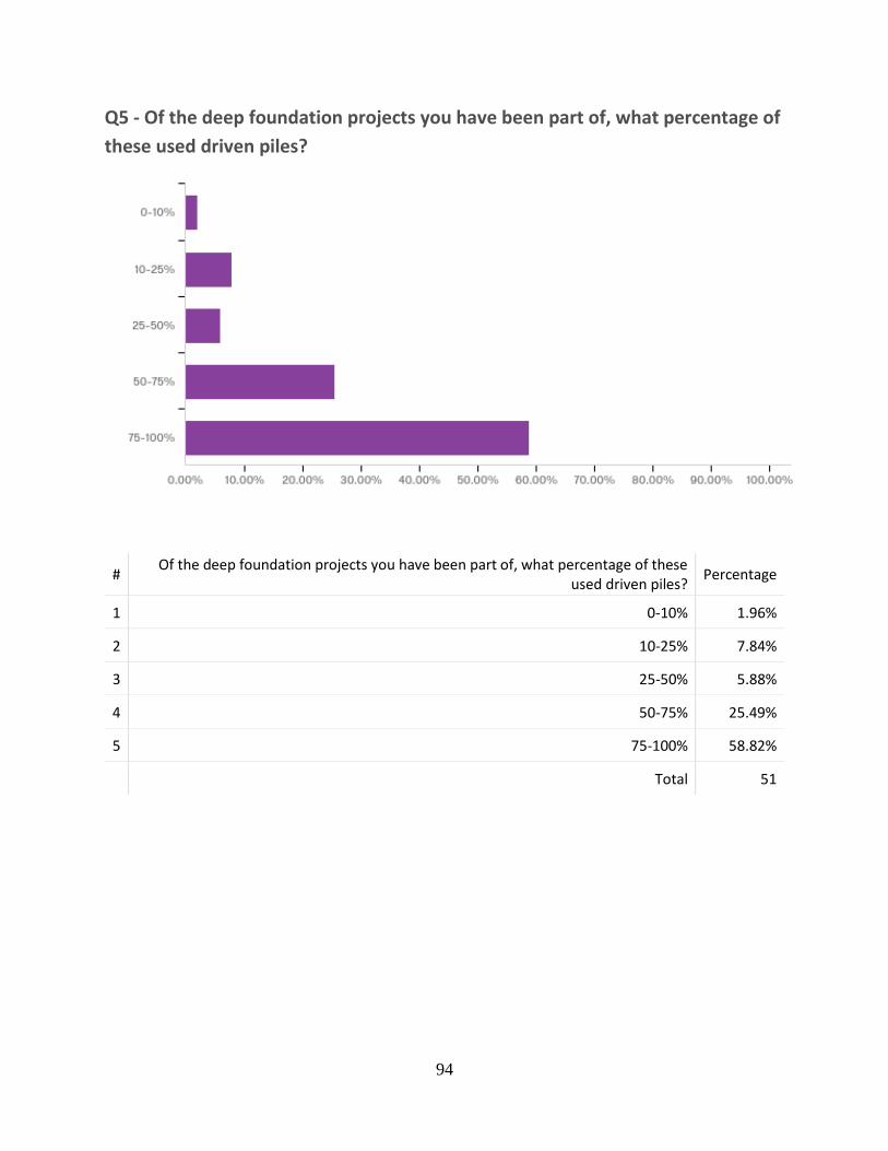
94
Q5 - Of the deep foundation projects you have been part of, what percentage of
these used driven piles?
# Of the deep foundation projects you have been part of, what percentage of these
used driven piles? Percentage
1 0-10% 1.96%
2 10-25% 7.84%
3 25-50% 5.88%
4 50-75% 25.49%
5 75-100% 58.82%
Total 51

95
Q6 - What is the most common type of driven pile used on projects you have
been involved in?
# What is the most common type of driven pile used on projects you have been
involved in? Percentage
1 H-pile 15.69%
2 Closed end pipe pile 0.00%
3 Open end pipe pile 17.65%
4 Precast prestressed concrete pile 41.18%
5 Timber pile 25.49%
Total 51

96
Q7 - Are you aware of the additional gain in pile capacity over time known as
"set-up"?
# Are you aware of the additional gain in pile capacity over time known as "set-up"? Percentage
1 Yes 90.20%
2 No 3.92%
3 Somewhat 5.88%
Total 51

97
Q8 - How often has set-up been explicitly incorporated into the driven pile
design on any of your projects for cost benefits?
# How often has set-up been explicitly incorporated into the driven pile design on any
of your projects for cost benefits? Percentage
1 Often 37.25%
2 Sometimes 15.69%
3 Rarely 23.53%
4 Never 15.69%
5 Unknown 7.84%
Total 51

98
Q9 - When set-up was incorporated, how was it suggested (select all that
apply)?
# When set-up was incorporated, how was it suggested (select all that apply)? -
Selected Choice Percentage
1 In the bid package 11.32%
2 In the soils report 54.72%
3 Contractor recommendation 9.43%
4 Other 24.53%
Total 53
Other
Other - Text
AFTER A TEST PILE
During construction
post-bid by geotechnical engineer
As a part of a static load test program

99
N/A
Not incorporated
After construction in cases where expected soil capacity could not be achieved and where soils were suitable to consider set-up
In field testing when nominal capacity was not obtained
NEVER SUGGESTED
Accounted for during pile load tests
We obtain pile capacities from geotechnical reports. Not sure how often geotechnical engineers consider set-up when calculating capacities. When calculated capacities are adjusted after a load test, the load test result benefits from a 14-day setup period.

100
Q10 - How much long-term increase in capacity (set-up) would you expect to
experience for piles driven in clayey soil in your region after a period of 3
months when compared to the end of drive capacity?
# How much long-term increase in capacity (set-up) would you expect to experience
for piles driven in clayey soil in your region after a period of 3 months when compared to the end of drive capacity?
Percentage
1 0-5% 0.00%
2 5-10% 11.76%
3 10-25% 11.76%
4 25-50% 19.61%

101
5 50-75% 9.80%
6 75-100% 9.80%
7 Greater than 100% 7.84%
8 Cannot generalize 21.57%
9 Unknown 7.84%
Total 51
Q11 - How much long-term increase in capacity (set-up) would you expect to
experience for piles driven in sandy soil in your region after a period of 3
months?

102
# How much long-term increase in capacity (set-up) would you expect to experience
for piles driven in sandy soil in your region after a period of 3 months? Percentage
1 0-5% 21.57%
2 5-10% 17.65%
3 10-25% 13.73%
4 25-50% 11.76%
5 50-75% 1.96%
6 75-100% 3.92%
7 Greater than 100% 3.92%
8 Cannot generalize 15.69%
9 Unknown 9.80%
Total 51

103
Q12 - Typically, how long after piles are driven are they subjected to the initial
loads of the superstructure (i.e. building skeleton, bridge girders, etc.)?
Please specify - Text Percentage
> 30 days, usually several months 2.04%
1 - 2 weeks 2.04%
1 to 2 months 2.04%
1 to 3 months 2.04%
1-2 months 2.04%
18 months 2.04%
2 weeks to 2 months 2.04%
2 weeks to 6 months (varies greatly with type of structure) 2.04%
2 weeks to a month 2.04%
2-3 months 4.08%
2-6 months. This is just a function of schedule 2.04%
3 months 4.08%
3 months to 9 months depending on project schedule. 2.04%
3 months to a year 2.04%
3 to 5 days 2.04%
3 to 6 months 2.04%
3-5 months 2.04%
30 days 2.04%
30+ days 2.04%
30-45 DAYS 2.04%
30-60 days 2.04%
4 weeks 2.04%
6 months 8.16%

104
6-months 2.04%
60 days 2.04%
7-14 days 2.04%
8 months 2.04%
A couple months 2.04%
A few months 2.04%
approximately 60 to 90 days on average 2.04%
couple months 2.04%
Less than 4 days 2.04%
Min. 14 days. recommended 2.04%
min. three months 2.04%
Months maybe 3 or more 2.04%
Mooring Piles 7 days 2.04%
more than a week 2.04%
ONE MONTH 2.04%
Two weeks 4.08%
Typically after the piling contractor is complete with the area 2.04%
unknown 4.08%
Years. Depends on when the next Hurricane hits South Louisiana. 2.04%
Total 49

105
Q13 - What percentage of projects utilized test piles, monitor piles, or indicator
piles for either static testing or dynamic analysis?
# What percentage of projects utilized test piles, monitor piles, or indicator piles for
either static testing or dynamic analysis? Percentage
1 0-10% 21.57%
2 10-25% 11.76%
3 25-50% 13.73%
4 50-75% 21.57%
5 75-100% 31.37%
Total 51

106
Q14 - Typically, how long after installation of a test pile is a static load
conducted?
# Typically, how long after installation of a test pile is a static load conducted? -
Selected Choice Percentage
1 1-3 days 3.92%
2 3-6 days 3.92%
3 1 week 31.37%
4 2 weeks 43.14%
5 Other 17.65%
Total 51
Other - Text Percentage
1 to 2 weeks 14.29%
21 days 14.29%
30 days 14.29%
Do not apply static load 14.29%

107
Don't know 14.29%
N/A 14.29%
Not performed 14.29%
Total 7
Q15 - If dynamic tests are conducted to verify design capacity, what percentage
of production piles are typically tested?
# If dynamic tests are conducted to verify design capacity, what percentage of
production piles are typically tested? Percentage
1 1-5% 59.57%
2 5-10% 36.17%
3 10-25% 4.26%
4 25-50% 0.00%
5 50-75% 0.00%
6 75-100% 0.00%
Total 47

108
Q16 - Considering that set-up continues over time, what do you feel is an
appropriate waiting time after test pile driving to verify design capacities before
production pile driving through static/dynamic load testing?
# Considering that set-up continues over time, what do you feel is an appropriate
waiting time after test pile driving to verify design capacities before production pile driving through static/dynamic load testing? - Selected Choice
Percentage
1 One day 4.00%
2 One week 16.00%
3 Two weeks 30.00%
4 One month 30.00%
5 Other 20.00%
Total 50
Other - Text Percentage
as long as schedule and budget permits but not less than 3 days 11.11%
Depends on soil sensitivity 11.11%
depends on the soil type 11.11%

109
Depends on the soil type, the type strucutre, and the urgency of the project 11.11%
ideally, would like to test at 14 days and then 28 days 11.11%
If I understand the question correctly, no time is required if the design capacity/length is confirmed by re-strike of the test pile.
11.11%
Multiple Times, 1 Day, 7 Day, 28 Day 11.11%
Static 2 to 4 weeks PDA shows log like increases. Do not have to wait as long 11.11%
This would depend on the project schedule. 11.11%
Total 9

110
Q17 - How much actual time typically elapses after pile driving until an end of
drive (EOD) test?
# How much actual time typically elapses after pile driving until an end of drive (EOD)
test? - Selected Choice Percentage
1 One minute 8.89%
2 5 minutes 8.89%
3 10 minutes 6.67%
4 15 minutes 15.56%
5 20 minutes 11.11%
6 Other 48.89%
Total 45

111
Other - Text Percentage
1 to 2 hours in clay soils 5.26%
1 week 5.26%
12 hours 5.26%
24 HOURS 5.26%
24 hr. and 14 day restrikes on indicator and 24hours on monitor piles. 5.26%
Do not perform an EOD 5.26%
don't know 5.26%
End of drive tests are performed during the intial driving of the pile. This usually takes about 5 to 20 minutes depending on soils.
5.26%
have been noticing an average of about 30 mins to 1 hr for conc piles 5.26%
immediate 5.26%
N/A 5.26%
never done one 5.26%
None, EOD is testing during installation 5.26%
Not sure 5.26%
Some are five-ten minutes, but typically most have been an hour lately. 5.26%
unknown 5.26%
varies 10.53%
varies on soil, pile type, pile length, and equipment used 5.26%
Total 19

112
Q18 - How often has a pile design been made more cost efficient (reduced
length, size or number) after obtaining results from a test pile?
# How often has a pile design been made more cost efficient (reduced length, size or
number) after obtaining results from a test pile? Percentage
1 Always 0.00%
2 Most of the time 19.61%
3 About half the time 13.73%
4 Sometimes 50.98%
5 Never 15.69%
Total 51

113
Q19 - How likely would you be to use an empirical formula to predict the future
capacity of a pile due to set-up and include in a design?
# How likely would you be to use an empirical formula to predict the future capacity of
a pile due to set-up and include in a design? Percentage
1 Extremely likely 0.00%
2 Moderately likely 29.63%
3 Neither likely nor unlikely 25.93%
4 Moderately unlikely 33.33%
5 Extremely unlikely 11.11%
Total 27

114
Q20 - How likely would you be to use an empirical formula to predict the future
capacity of a pile due to set-up and include in an alternate proposal (e.g. value
engineering)?
# How likely would you be to use an empirical formula to predict the future capacity of
a pile due to set-up and include in an alternate proposal (e.g. value engineering)? Percentage
1 Extremely likely 12.50%
2 Moderately likely 25.00%
3 Neither likely nor unlikely 20.83%
4 Moderately unlikely 33.33%
5 Extremely unlikely 8.33%
Total 24

115
Q21 - How likely is it to lengthen overall project schedules to take advantage of
pile set-up if a decrease in cost could be achieved?
# How likely is it to lengthen overall project schedules to take advantage of pile set-up
if a decrease in cost could be achieved? Percentage
1 Extremely likely 0.00%
2 Somewhat likely 38.00%
3 Neither likely nor unlikely 20.00%
4 Somewhat unlikely 32.00%
5 Extremely unlikely 10.00%
Total 50

116
Q22 - How likely is it to reorganize project schedules (but maintain the overall
duration) to take advantage of pile set-up if a decrease in cost could be
achieved?
# How likely is it to reorganize project schedules (but maintain the overall duration) to
take advantage of pile set-up if a decrease in cost could be achieved? Percentage
1 Extremely likely 8.00%
2 Somewhat likely 50.00%
3 Neither likely nor unlikely 24.00%
4 Somewhat unlikely 12.00%
5 Extremely unlikely 6.00%
Total 50

117
Q23 - Rank the following methods for design verification that are most
common. Drag the terms to put them in rank order, with the top term being the
most common.
# Field Minimum Maximum Mean Std
Deviation Variance Count
1 Dynamic formula 1.00 5.00 3.12 0.96 0.92 49

118
2 Wave Equation (WEAP)
analysis 1.00 4.00 2.47 1.13 1.27 49
3 Dynamic tests 1.00 4.00 2.37 0.90 0.80 49
4 Static tests 1.00 4.00 2.08 1.24 1.54 49
5 Other 3.00 5.00 4.96 0.28 0.08 49
# Question 1 2 3 4 5 Total
1 Dynamic formula 4.08% 26.53% 24.49% 42.86% 2.04% 49
2 Wave Equation (WEAP) analysis 30.61% 12.24% 36.73% 20.41% 0.00% 49
3 Dynamic tests 14.29% 48.98% 22.45% 14.29% 0.00% 49
4 Static tests 51.02% 12.24% 14.29% 22.45% 0.00% 49
5 Other 0.00% 0.00% 2.04% 0.00% 97.96% 49

119
Q24 - Rank the following methods for construction control that are most
common in your practice. Drag the terms to put them in rank order, with the
top term being the most common.
# Field Minimum Maximum Mean Std
Deviation Variance Count
1 Dynamic formula 1.00 5.00 3.23 1.00 1.01 48

120
2 Wave Equation (WEAP)
analysis 1.00 4.00 2.40 1.06 1.11 48
3 Dynamic tests 1.00 4.00 2.25 0.97 0.94 48
4 Static tests 1.00 4.00 2.23 1.19 1.43 48
5 Other 1.00 5.00 4.90 0.59 0.34 48
# Question 1 2 3 4 5 Total
1 Dynamic formula 4.17% 25.00% 18.75% 47.92% 4.17% 48
2 Wave Equation (WEAP) analysis 29.17% 16.67% 39.58% 14.58% 0.00% 48
3 Dynamic tests 25.00% 37.50% 25.00% 12.50% 0.00% 48
4 Static tests 39.58% 20.83% 16.67% 22.92% 0.00% 48
5 Other 2.08% 0.00% 0.00% 2.08% 95.83% 48

121
Q25 - In your experience, which dynamic analysis method is most commonly
used?
# In your experience, which dynamic analysis method is most commonly used? Percentage
1 Wave Equation analysis 10.20%
2 Dynamic tests with pile driving analyzer (PDA) 40.82%
3 Dynamic test with PDA and signal matching software (i.e. CAPWAP) 48.98%
Total 49

122
Q26 - Have you ever incorporated set-up into a driven pile design?
# Have you ever incorporated set-up into a driven pile design? Percentage
1 Yes 51.85%
2 No 48.15%
Total 27

123
Q27 - What analysis method do you use for the preliminary design of driven
piles?
# What analysis method do you use for the preliminary design of driven piles? -
Selected Choice Percentage
1 Static analysis 64.00%
2 Dynamic formulas 12.00%
3 Dynamic tests 8.00%
4 Static tests 4.00%
5 Other 12.00%
Total 25
Other - Text Percentage
Not a geotech 50.00%
We do not design 50.00%
Total 2

124
Q28 - Which dynamic formula do you use most often?
# Which dynamic formula do you use most often? - Selected Choice Percentage
1 Engineering News (EN) formula 26.09%
2 Gates formula 13.04%
3 Modified Gates formula 26.09%
4 Hiley formula 0.00%
5 Other 34.78%
Total 23
Other - Text Percentage
? 14.29%
N/A 14.29%
None 42.86%

125
Test Results of the Dynamic Tests/CAPWAP 14.29%
We do not design 14.29%
Total 7
Q29 - What percentage of projects do you only use static analysis for
determining pile length?
# What percentage of projects do you only use static analysis for determining pile
length? Percentage
1 0-10% 20.00%
2 10-25% 24.00%
3 25-50% 28.00%
4 50-75% 8.00%
5 75-100% 20.00%
Total 25

126
Q30 - Which static analysis method do you use most often?
# Which static analysis method do you use most often? Percentage
1 Alpha method 25.00%
2 Beta method 10.00%
3 Gamma method 0.00%
4 Nordlund-Thurman method 25.00%
5 CPT method 20.00%
6 SPT method 20.00%
Total 20

127
Q31 - What design method do you typically use for driven pile design?
# What design method do you typically use for driven pile design? Percentage
1 LRFD 63.16%
2 LFD 0.00%
3 ASD 36.84%
Total 19

128
Q32 - What percentage of projects use LRFD design methodology?
# What percentage of projects use LRFD design methodology? Percentage
1 0% 15.00%
2 1-10% 5.00%
3 10-25% 20.00%
4 25-50% 25.00%
5 50-75% 10.00%
6 75-100% 25.00%
Total 20

129
Q33 - For projects where you use LRFD, how is the resistance factor
determined?
# For projects where you use LRFD, how is the resistance factor determined? -
Selected Choice Percentage
1 AASHTO recommended value 38.89%
2 Regionally calibrated value 33.33%
3 Other 27.78%
Total 18
Other - Text Percentage
Both of the above 25.00%
Current DOTD recommended factors 25.00%
N/A 25.00%
NA 25.00%
Total 4

130
Q34 - How likely or confident would you be using set-up prediction methods in
your design of driven piles?
# How likely or confident would you be using set-up prediction methods in your design
of driven piles? Percentage
1 Extremely likely 13.04%
2 Moderately likely 39.13%
3 Slightly likely 30.43%
4 Neither likely nor unlikely 4.35%
5 Slightly unlikely 8.70%
6 Moderately unlikely 4.35%
7 Extremely unlikely 0.00%
Total 23

131
VITA
Kelsey Herrington was born and raised in Metairie, Louisiana, and received her bachelor’s
degree in Civil Engineering from Louisiana State University (LSU) in May 2015. Following
graduation, she worked at an environmental engineering consulting firm and her interest in
structural engineering began. She next worked for another consulting firm on the disaster relief
program following the Baton Rouge flooding of 2016. She then decided she wanted to further
her education and gain experience in structural engineering by returning to LSU to obtain a
Master’s Degree in Civil Engineering with an emphasis on structural engineering.