integrating vehicle routing and driver...
TRANSCRIPT

UNIVERSITY OF GHENT
FACULTY OF ECONOMICS AND BUSINESS ADMINISTRATION
ACADEMIC YEAR 2010 – 2011
INTEGRATING VEHICLE ROUTING AND DRIVER SCHEDULING
Master thesis presented to obtain the degree of
Master in Applied Economic Sciences: Business Engineering
Jannick Staes
under the leadership of
Prof. dr. ir. Birger Raa

iv
- PERMISSION
Ondergetekende verklaart dat de inhoud van deze masterproef mag geraadpleegd en/of
gereproduceerd worden, mits bronvermelding.
The author declares that the content of this master’s thesis may be consulted and/or
reproduced, with acknowledgement.
Jannick Staes

Word of Thanks
During the constitution of this master’s thesis, many people have helped me in one way
or another and have contributed to this work. I would like to pay attention to them in
this section.
First of all, I would like to thank my promotor, prof. B. Raa. His advice during difficult
moments and the many helpful cues on his part have been invaluable to make this work.
A special mention goes out to Onne Beek, Daan De Witte and Sander Van der Meulen
who have provided me with advice and proofread the work before you.
Lastly I would like to thank my parents and friends who have supported me during the
many months it took for this work to be created.
Thank you,
Jannick Staes
v

Contents
Word of Thanks v
1 Introduction 3
2 The Vehicle Routing Problem 5
2.1 Introduction . . . . . . . . . . . . . . . . . . . . . . . . . . . . . . . . . . . 5
2.2 Problem Definition . . . . . . . . . . . . . . . . . . . . . . . . . . . . . . . 7
3 Literature review 11
3.1 Vehicle Routing Problem with Time Windows . . . . . . . . . . . . . . . . 11
3.2 Driver Regulations in the European Union . . . . . . . . . . . . . . . . . . 12
3.2.1 Regulation (EC) No. 561/2006 on Driving Hours . . . . . . . . . . 12
3.2.2 Directive 2002/15/EC on Working Hours . . . . . . . . . . . . . . 15
3.3 VRPTW with Driver Regulations . . . . . . . . . . . . . . . . . . . . . . . 16
3.4 Vehicle Routing Problem with Compartments . . . . . . . . . . . . . . . . 27
3.5 Contribution . . . . . . . . . . . . . . . . . . . . . . . . . . . . . . . . . . 28
4 Solution Approach 30
4.1 Restricted Dynamic Programming . . . . . . . . . . . . . . . . . . . . . . 30
4.2 Break and Rest Scheduling . . . . . . . . . . . . . . . . . . . . . . . . . . 33
4.3 Multiple Compartments Method . . . . . . . . . . . . . . . . . . . . . . . 36
vi

Contents vii
5 Computational Results 39
5.1 Restricted Dynamic Programming for the VRPTW . . . . . . . . . . . . . 40
5.2 Driver Rules . . . . . . . . . . . . . . . . . . . . . . . . . . . . . . . . . . . 41
5.3 Multiple Compartments . . . . . . . . . . . . . . . . . . . . . . . . . . . . 42
5.4 Multiple Compartments and Driver Rules . . . . . . . . . . . . . . . . . . 44
6 Conclusion 46
A Pseudo Code 49
A.1 Basic Method for the VRPTW . . . . . . . . . . . . . . . . . . . . . . . . 50
A.2 Break and Rest Scheduling Method . . . . . . . . . . . . . . . . . . . . . . 51
A.3 Multiple Compartments . . . . . . . . . . . . . . . . . . . . . . . . . . . . 51
B Detailed Computational Results 55
Bibliography 61
Nederlandstalige Samenvatting
In dit werk wordt het Vehicle Routing Problem (VRP) behandeld. In dit probleem
hebben we als doel om een bepaald aantal klanten, elk met een eigen vraag naar een
bepaald product, te bedienen met zo weinig mogelijk voertuigen en met zo weinig mo-
gelijk afgelegde afstand. Deze klanten zijn vaak rond een centraal depot uitgespreid.
Verder worden er meerdere beperkingen aan dit probleem opgelegd en besproken. Een
eerste vorm is het bestaan van tijdsvensters bij klanten waarbij een voertuig verplicht
is om een levering bij de klant in een vooraf bepaalde tijdsperiode te maken. Dit komt
erg veel voor in de praktijk en is dan ook ruim besproken in de literatuur. Verder is het
ook belangrijk dat ten allen tijde de Europese wetgeving rond pauzes en rust periodes
voor chauffeurs gevolgd wordt. Deze beperking is pas erg recentelijk geıntroduceerd in
de literatuur en is bijgevolg ook weinig bestudeerd.
Als laatste beperking bekijken we ook het geval waarbij klanten een levering wensen van
meerdere verschillende producten die niet in eenzelfde ruimte kunnen vervoerd worden.
Dit komt veel voor in enerzijds de voedselindustrie waarbij diepvries producten apart
moeten vervoerd worden en anderzijds in de petroleum industrie waarbij de verschillende
soorten benzine nooit gemengd mogen worden. Ook andere sectoren kunnen hiervan ge-
bruik maken, zo kunnen verschillende bedrijven hetzelfde distributienetwerk gebruiken
om synergieen te bereiken. In elk geval moeten de voertuigen in meerdere compar-
timenten opgedeeld worden waarbij producten niet gemengd mogen worden. Ook dit
probleem heeft tot recentelijk erg weinig aandacht gekregen in de literatuur.
1

Contents 2
In deze thesis presenteren wij een methode om op een eenvoudige manier om te gaan
met de bovenstaande beperkingen. Wij gebruiken het Restricted Dynamic Programming
model geıntroduceerd door Gromicho et al. (2009) en tonen aan dat dit model uitermate
geschikt is om om te gaan met eeb VRP met veel beperkingen. Alhoewel dit model
niet kan concurreren met geavanceerde local search technieken, bekomen we wel goede
resultaten als we de Europese regelgeving en meerdere compartimenten beschouwen. We
tonen verder aan dat het incorporeren van deze beperkingen enkel leidt tot respectievelijk
40% en 60% langere computationele tijden.
Chapter 1
Introduction
As a master student in business engineering, the choice of a subject for a master’s
thesis lies wide open. One can choose to create a work in many different sciences, yet
my interest went out to a subject in the area of Operations Management. The chosen
subject deals with a rich vehicle routing problem which I find to be very intriguing
because of its practical relevance.
In this work, the vehicle routing problem with time windows is investigated and expanded
in two ways. Firstly, methods are presented to include European legislation concerning
driver rules into the vehicle routing problem. Furthermore, another constraint called
multiple compartments is added to observe the effect of customers with demand for two
heterogeneous products. This is done by using an approach called restricted dynamic
programming which allows for a relatively easy addition of constraints to the vehicle
routing problem.
The remainder of this thesis is structured as follows. Chapter 2 gives an overview of
the Vehicle Routing Problem, both in a qualitative and quantitative way. Chapter 3
will provide an overview of current existing literature with emphasis on research that
has dealt with driver rules and multiple compartments and explain our contribution to
the research in these areas. Furthermore this chapter will provide a summary of the
European Union legislation regarding driver rules. Chapter 4 will explain our solution
3

Chapter 1. Introduction 4
approach in detail, whereas chapter 5 will present our computational results based on
this method. Finally, in chapter 6, a conclusion is presented. The pseudo code of the
solution approach and detailed tables of the computational results can be found in the
appendices.

Chapter 2
The Vehicle Routing Problem
2.1 Introduction
Transportation is a crucial part of human economic activity. Whether we want to visit
friends and family, buy food or browse the internet, we consume services of a system
that transports people, physical goods or information. As such, it takes up a large part
of our economic activities. Rodrigues et al. (2005) have estimated that global logistics
expenditures represent 13.8% of the world GDP in the year 2002. In Belgium, this figure
amounted to 12.1%. Furthermore, road transportation remains the predominant mode
for freight transport. According to Eurostat (Huggins, 2009) 45.6% of all goods transport
in the European Union happens by road with sea transport coming in second at 37.3%.
These data clearly underline the importance of routing problems to the economy.
A Vehicle Routing Problem (or Vehicle Scheduling Problem) (VRP) is in essence a ques-
tion of how to distribute goods from central depots to customers. The various algorithms
developed in order to solve these problems can be applied to many different real-life ap-
plications. Next to problems dealing with the distribution and/or pickup of goods, they
can also be applied to problems such as waste collection or bus routing. The problem
was first introduced in Dantzig and Ramser (1959) where the authors presented a model
for the routing of gasoline trucks between a terminal and service stations. Since then,
5

Chapter 2. The Vehicle Routing Problem 6
numerous variants of the original VRP have been introduced. In this section we will
limit ourselves to a description of the Capacitated VRP (CVRP) and the VRP with
Time Windows (VRPTW) (cfr. infra). A discussion of other important variants can be
found in Toth and Vigo (2002).
In any VRP, we are presented with a set of vehicles with designated drivers that have
to service a number of customers. These vehicles can belong to one or multiple central
depots. We want to obtain a set of routes, one for each vehicle, that determines the order
in which the vehicle has to service a certain set of customers and thus also determines
the route of the vehicle on the road network. These set of routes should be designed
in such a way that they fulfill all the customer requirements and adhere to all the
operational constraints we have imposed on the problem. The objective is to minimize
the total transportation cost. In practice, this usually means that the primary objective
is to minimize the number of vehicles and as a secondary objetive, minimize the total
distance traveled.
The road network on which the routes take place are often represented by a graph
where the arcs are road sections and the vertices are the depot and customer locations.
Both a travel distance and travel time are associated with each arc. An arc between
two customers or between a customer and the depot always relates to the shortest path
between the two nodes. Every customer has a few characteristics such as the coordinates
in the graph, time required to service the customer, its demand and its time windows.
These last two are critical constraints in the CVRP and VRPTW respectively. Vehicles
are characterized by their home depot (although it is possible to end service at another
depot), their capacity and costs associated with the usage of the vehicle (such as fuel
consumption rate).
In this thesis, we will discuss two important constraints in practical VRPs: driver reg-
ulations and multiple compartments per vehicle. Legislation stipulates certain rules to
which all drivers have to adhere. An overview of these stipulations can be found in
chapter 4. These rules have to be taken into account for real-life applications. Some

Chapter 2. The Vehicle Routing Problem 7
authors (Prescott-Gagnon et al., 2010) have labeled this the VRPTW with driver rules
(VRPTWDR). Multiple compartments on the other hand are needed for VRPs where
there is a demand for multiple products which can not all be stored in the same envi-
ronment. This mainly occurs in sectors such as petrol distribution where different types
of petrol can never be mixed and food distribution where refrigerated products have to
kept in a different freezing compartment of the truck. Furthermore, recent trends in
Supply Chain Management (Mason et al., 2007) have shown an increased use of horizon-
tal collaboration in which different firms transport goods via collaborating their routing
and may need to use multiple compartments.
Any solution to a VRP also has to conform to certain operational constraints. In the
VRPTW, this means that each vehicle can never transport more than its capacity and
that every customer has to be visited within his or her time window. Other variants may
pose other constraints such as precedence relations in the pickup and delivery problem.
2.2 Problem Definition
In this section, we will present a mathematical problem formulation for the VRPTW
which was introduced by Toth and Vigo (2002). This problem is NP-hard, even finding
a feasible solution with a fixed amount of vehicles is NP-complete (Savelsbergh, 1985).
The VRPTW can be described as a graph problem with G = (V,A) a complete graph
where V = {0, . . . , n} is the set of vertices and A is the arc set. In this graph, given a
vertex i, ∆+(i) represents the forward star of i, which is the set of vertices j such that
each arc (i, j) ∈ A. In other words, the forward star defines the vertices that are directly
reachable from i. Likewise, ∆−(i) is the backward star of i and defines the set of vertices
j such that each arc (j, i) ∈ A or the vertices from which i is directly reachable.
There is a travel cost associated for every arc (i, j) ∈ A and is represented by a non-
negative cost cij . In most instances, each vertex has a set of coordinates and arcs
between vertices can be calculated as the Euclidian distance between them. Each cus-

Chapter 2. The Vehicle Routing Problem 8
tomer i(i = 1, . . . , n) has a nonnegative demand di to be delivered (or picked up). This
can be done by using a set of K identical vehicles, each with capacity C. In order to
create feasible solutions, the total demand can not be lower than the total capacity and
no specific customer demand can exceed C.
In the CVRP we want to find a set of K routes, where we want to have K as small as
possible and minimize the sum of the travel costs associated with the arcs traveled by
the circuits. Furthermore, the following constraints apply:
� Each circuit starts and ends at the depot vertex,
� Each customer is visited by just one circuit,
� The sum of all the customer demands along a circuit cannot exceed the vehicle
capacity C.
In the VRPTW we impose an additional constraint where each customer has a time
window represented by the time interval [ai, bi], where ai is often called the ready time
and bi the due date of the customer. We also associate a travel time tij with every arc
(i, j) ∈ A and a service time si with each customer. Travel times are often calculated by
dividing the length of an arc by the travel speed of the vehicle in question. The start of
service must happen in the time interval and the vehicle must remain at the customer for
the duration of the service time. If the vehicle arrives at the customer before the start
of its time window, it must wait until the ready time of the customer. Likewise, service
cannot start after the due date is exceeded. As such, we can add another constraint to
the ones postulated in the previous paragraph:
� For every customer, service has to happen within the time interval [ai, bi] and must
take si time periods.
The following model is based on a multicommodity network flow formulation. Here,
the depot is represented by two nodes: 0 and n + 1. As such, every vehicle starts at

Chapter 2. The Vehicle Routing Problem 9
0 and ends at node n + 1. This allows us to define N as V \{0, n + 1}. The depot
has a time window of [E,L] with E the earliest time a vehicle can start at the depot
and L the latest time a vehicle can arrive back at the depot. The model starts with a
predetermined amount of K vehicles. If less vehicles are used, we can implement this
by adding an additional arc to A: (0, n + 1) with c0,n+1 = t0,n+1 = 0. In the model
two types of variables are present: on the one hand flow variables xijk, (i, j) ∈ A, k ∈ K
which are equal to 1 if the arc between i and j is used by vehicle k and 0 otherwise,
on the other hand time variables wik, i ∈ V, k ∈ K which specify the start of service at
customer i by vehicle k.
min∑k∈K
∑(i,j)∈A
cijxijk (2.1)
subject to
∑k∈K
∑j∈∆+(i)
xijk = 1 ∀ i ∈ N, (2.2)
∑j∈∆+(0)
x0jk = 1 ∀ k ∈ K, (2.3)
∑i∈∆−(j)
xijk −∑
i∈∆+(j)
xjik = 0 ∀ k ∈ K, j ∈ N, (2.4)
∑i∈∆−(n+1)
xi,n+1,k = 1 ∀ k ∈ K, (2.5)
xijk(wik + si + tij − wjk) ≤ 0 ∀ k ∈ K, (i, j) ∈ A, (2.6)
ai∑
j∈∆+(i)
xijk ≤ wik ≤ bi∑
j∈∆+(i)
xijk ∀ k ∈ K, i ∈ N, (2.7)
E ≤ wik ≤ L ∀ k ∈ K, i ∈ {0, n+ 1}, (2.8)∑i∈N
di∑
j∈∆+(i)
xijk ≤ C ∀ k ∈ K, (2.9)
xijk ∈ {0, 1} ∀ k ∈ K, (i, j) ∈ A. (2.10)
The objective function 2.1 expresses the total cost which is to be minimized. Constraint
2.2 restricts the customer to one route and vehicle. Constraints 2.3 - 2.5 define the

Chapter 2. The Vehicle Routing Problem 10
flow of vehicles: each vehicle can only reach one customer immediately after the depot,
can only visit customers sequentially and can only return to the depot from the last
customer.
Constraints 2.6 - 2.8 guarantee feasibility concerning time windows. The first makes
sure that the start of service at a customer can only happen after the start of service at
the previous customer added with the service time and travel time to the next customer.
Equation 2.7 guarantees that start of service at customer i happens during the time
window while also forcing wik = 0 when customer i is not visited by vehicle k. Equation
2.8 forces any vehicle to depart and arrive at the depot during the time window of the
depot, this of course implies that all other service time starts are limited by [E,L].
The next constraint (2.9) is the capacity constraint: the total demand of the customers
visited by a vehicle k must not be higher than C. Finally, the last constraint imposes
binary restrictions on the flow variables.

Chapter 3
Literature review
3.1 Vehicle Routing Problem with Time Windows
Both the classical VRP as the VRPTW have been subject to intensive research over the
years. The problem was first formulated by Dantzig and Ramser (1959) where gasoline
trucks had to service a number of stations without exceeding their capacity. The authors
presented the problem as a variant of the Traveling Salesman Problem (TSP) where the
routing of trucks could be seen as a TSP with multiple salesmen and with deliveries
at each location. In order to distinguish this problem from its variants, it was later
dubbed as the Capacitated Vehicle Routing Problem (CVRP). The most comprehensive
overview of the VRP can be found in the book by Toth and Vigo (2002). Next to a
thorough description of the problem, the authors present the current state of branch-
and-bound, brand-and-cut and (meta)heuristic approaches to the problem. They also
exhibit algorithms for some of the more well-known variants of the VRP: the VRPTW,
the VRP with backhauls and the pickup and delivery problem.
The VRPTW is the most well-known variant of the CVRP and consequently has been
studied intensively. Kallehauge et al. (2005) provide an overview of exact algorithms
designed for the VRPTW. Most of the research, however, has been performed on heuristic
approaches. This is both due to the high complexity of the problem as well to its wide
11

Chapter 3. Literature review 12
applicability to real-life business sitations. Braysy and Gendreau compiled an overview
of the heuristic approaches to the VRPTW, both for route construction and local search
algorithms (Braysy and Gendreau, 2005a) and for metaheuristics (Braysy and Gendreau,
2005b).
3.2 Driver Regulations in the European Union
In the European Union, rules concerning working hours of drivers are postulated by EC
regulation 561/2006 since 2007. This legislative act restricts maximum driving hours
during workdays and workweeks and determines the length of required break and rest
periods. It also states employers will be held responsible for infringements. Compliance
to the regulation is thus of the utmost importance to the employer faced with a routing
problem.
As Kok et al. (2010) pointed out, these are not the only rules that need to be considered
when scheduling drivers. Directive 2002/15/EC on Working Hours specifies restrictions
on total working hours for workers. This means that tasks such as loading and unloading
cargo, filling in administration or assisting passengers should be added to driving time
to obtain the total amount of working hours for the driver. In our solution approach,
we will group these tasks together in one concept: service time. Waiting times will not
be considered since we will consider a deterministic VRP in which all waiting times will
be known in advance.
In the next sections we will summarize these regulations into a few concise and easy to
understand rules.
3.2.1 Regulation (EC) No. 561/2006 on Driving Hours
In this section, we will follow the summary first introduced by Goel (2009) who postu-
lated 9 rules as follows:
1. After driving for four-and-a-half hours, the driver will take an uninterrupted break

Chapter 3. Literature review 13
of at least 45 minutes. This is not needed if the driver takes a rest period.
2. The time between two rest periods (a day basically) cannot contain more than nine
hours of driving time. A rest period should be at least 11 hours long.
3. In the 24 hours after the end of a daily rest period, the driver will have taken a
new daily rest.
4. The weekly driving time cannot exceed 56 hours.
5. A weekly rest period has to start no later than 144 hours (or 6 days) after the end
of the previous weekly rest period.
6. The daily driving time may be extended to at most 10 hours, but no more than
twice during the week.
7. The daily rest period may be reduced to nine hours but no more than three times
per week.
8. The break between driving periods can be replaced by a break of at least 15 minutes
followed by a break of at least 30 minutes.
9. The daily rest period may be split up in two periods: the first one must be an
uninterrupted period of at least three hours and the second an uninterrupted period
of at least nine hours.
Next to these rules, others exist for multimanning drivers, acculumated driving times
during consecutive weeks or the duration of weekly rest periods. These will however not
be discussed in this thesis. A typical work day schedule is shown in Figure 3.1. This
schedule is based on the first five rules we just described. The other four rules can be
viewed as extensions to the first five “core” rules. Figure 3.2 shows us a schedule in
which the driver drives an additional hour after another break and consequently takes
a shorter rest period, while Figure 3.3 illustrates rule 8 that allows a driver to split up
his break between driving sections in two shorter breaks.

Chapter 3. Literature review 14
Figure 3.1: Typical work day of a EU driver. (Goel, 2009)
Figure 3.2: Work schedule based on rule 6 and 7. (Goel, 2009)
As Goel (2010) pointed out, rules 6 through 9 can be seen as provisions in order to
increase flexibility for the drivers. If we take these rules into account when scheduling, we
may achieve further savings and maximise the productive time of both vehicle and driver.
On the other hand, the resulting tours can be very vulnerable to unexpected delays such
as traffic jams and can lead to missing time windows of subsequent deliveries. Both Kok
et al. (2010) and Prescott-Gagnon et al. (2010) report results on the effect on the decision
variables of these provisions. Kok et al. (2010) noticed a 4.28% reduction in the number
of vehicles used and 1.54% reduction of the total distance traveled. Prescott-Gagnon
et al. (2010) observed a much smaller effect, in their algorithm the effect amounts to
a 1.7% reduction in vehicles used and a 1.5% decrease in total distance. Furthermore,
Goel (2010) has shown that taking break periods in two parts such as in rule 8 and 9 only
brings a very marginal benefit (a 0.2% decrease in feasible schedules). As the benefits

Chapter 3. Literature review 15
Figure 3.3: Work schedule based on rule 8. (Goel, 2009)
of including these provisions in route scheduling are rather small yet may prove to be
invaluable in dealing with unexpected delays, we will not include these in our solution
approach in order to guarantee a certain level of robustness.
3.2.2 Directive 2002/15/EC on Working Hours
Directive 2002/15/EC can be seen as an additional restriction to be considered when
scheduling feasible routes and was first considered by Kok et al. (2010). As this Directive
provides regulations based on working times, this also applies to driving times. Next to
driving hours, this naturally also applies to activities such as loading and unloading, as-
sisting passengers, administrative work and waiting times where a driver cannot dispose
freely of his time. In this thesis, we will only consider driving times and service times at
the customer.
The following restrictions of the Directive affect the vehicle routing problem:
1. A working period cannot exceed six hours without break.
2. A working period is ended by a break of at least 30 minutes. If the total working
time between rest periods exceeds nine hours, a break of at least 45 minutes is
required. This break can be divided into parts of at least 15 minutes each.
3. The total weekly working time may not exceed 60 hours.
Although these rules seem less restrictive than Regulation (EC) No. 561/2006, it is still
possible to comply to the Regulation yet infringe the Directive. For example, if a driver
were to service a customer for 1 hour, drive 4.5 hours and service another customer, he

Chapter 3. Literature review 16
would be working 6.5 hours nonstop which is in violation with the Directive yet still
complies with the driver rules of Regulation No. 561/2006. In practice, both of these
regulations have to be followed at all times.
3.3 VRPTW with Driver Regulations
Compared to the VRPTW, this subproblem has received only very little attention in
the research community. Powell et al. (2000) took a maximum number of hours worked
during a tour into account in designing labeling algorithms for assigning drivers to a
certain set of tasks. Campbell and Savelsbergh (2004) took a similar approach where
a label was used to denote a shift time limit. In their insertion heuristic, a feasibility
check is included before inserting a new customer. Both these models are quite basic
and don’t incorporate any rest periods or breaks. Savelsbergh and Sol (1998) present a
real-life planning module implemented at a Dutch transport company confronted with
a pickup and delivery problem. In this case study, the model took night and lunch
breaks explicitly into account although no specific regulation was followed. The problem
was solved with a column generation method. In another case study of a practical
pickup and delivery problem, Xu et al. (2003) also use column generation in order to
solve the problem that takes US regulation on legal driver working hours into account.
Archetti and Savelsbergh (2009) present an algorithm for truck driver scheduling on
given sequences of customers complying with US regulation. These US rules are less
complicated compared to the EU legislation however.
The first effort regarding EU regulations was done by Goel (2009), in which the author
proposes a method complying with the first 5 rules of Regulation No.561/2006 which
we discussed in section 3.2. Goel proposes two methods to implement these regulations,
a naive method and a multilabel one. The naive method is summarized in figure 3.4.
Goel defines driving time between two nodes as δ and represents the state of the driver
at a node by a multidimensional label l = (larrival, ldaily, lnonstop). In this label, larrival
stands for the arrival time at the node, ldaily for the acculumated driving time since the
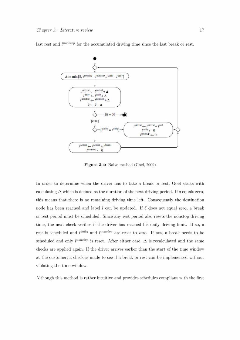
Chapter 3. Literature review 17
last rest and lnonstop for the accumulated driving time since the last break or rest.
Figure 3.4: Naive method (Goel, 2009)
In order to determine when the driver has to take a break or rest, Goel starts with
calculating ∆ which is defined as the duration of the next driving period. If δ equals zero,
this means that there is no remaining driving time left. Consequently the destination
node has been reached and label l can be updated. If δ does not equal zero, a break
or rest period must be scheduled. Since any rest period also resets the nonstop driving
time, the next check verifies if the driver has reached his daily driving limit. If so, a
rest is scheduled and ldaily and lnonstop are reset to zero. If not, a break needs to be
scheduled and only lnonstop is reset. After either case, ∆ is recalculated and the same
checks are applied again. If the driver arrives earlier than the start of the time window
at the customer, a check is made to see if a break or rest can be implemented without
violating the time window.
Although this method is rather intuitive and provides schedules compliant with the first

Chapter 3. Literature review 18
two rules of the legislation, it cannot guarantee to find feasible schedules. For example,
in certain cases it can be beneficial to schedule an “early” break or rest. In figure 3.5
the top schedule represents what the naive method would generate. This will lead to
the earliest handling yet the driver has to wait for 2 hours until he can begin. The
schedules below have no such unproductive work by implementing an earlier rest period
and handling the customer later in its time window. It is however impossible to deduce
at this point which schedule dominates the other as we need information of subsequent
driver activities.
Figure 3.5: Several alternative states can be feasible. (Goel, 2009)
Goel thus proposes a more sophisticated approach in which the different schedules can be
considered. This approach is summarized in figure 3.6. This method is able to generate
multiple schedules for each new node added and each is added to the label set ϕ. It
works similar to the naive method yet when δ > 0, ldaily < tdaily and the next driving
period is shorter than tnonstop, it might prove beneficial to schedule a rest period instead
of a break. The method creates a new label for this state and expands this label using
the same method. In the end, set ϕ contains multiple labels and after verifying if no
label is dominated by another, every label is expanded further. This obviously increases
complexity yet Goel reports that the multilabel method provides solutions which, on

Chapter 3. Literature review 19
average, contain 10% less vehicles and total distance.
Figure 3.6: Goel’s multilabel method which is capable of generating early rests and conse-
quently generates multiple labels for each node (Goel, 2009).
Finally Goel provides compliance with the third rule of the regulation (one full rest
per 24 hours) by extending the rest period if a driver would encounter waiting time
at subsequent customers and thus violate this rule. Furthermore, he complies with
rule 4 and 5 trivially by assuming that the sum of individual driving times between
customers cannot exceed the weekly working time and that each vehicle is only available
for 144 hours. Goel uses an insertion method by Antes and Derigs (1995) and a large
neighbourhood search by Shaw (1997) to obtain solutions for the Solomon instances.
These instances all have 100 customers and are divided into six categories. Instances
can be clustered(c), random(r) or semi-clustered(rc) and each category has instances with

Chapter 3. Literature review 20
small capacity vehicles (1) or large capacity vehicles (2). Goel’s results are summarized
in table 3.1. Since the large neighborhood search is random, each instance was solved
five times for 30 minutes each, where the multilabel approach was only able to perform
half as many iterations due to its increased complexity.
Table 3.1: Results of the naive and multilabel method by Goel.
Multilabel Naive
Problem Avg. vehicles Avg. distance Avg. vehicles Avg. distance
c1 12.04 1,096.58 13.91 1,300.82
c2 9.58 1,008.71 11.05 1,200.90
r1 11.93 1,180.96 12.95 1,280.76
r2 11.27 1,151.24 11.75 1,233.69
rc1 12.10 1,373.10 13.10 1,534.43
rc2 11.43 1,389.50 12.35 1,485.84
A second effort into the problem was provided by Kok et al. (2010). This is the first
paper to take all the rules of Regulation no. 561/2006 into account as well as restrictions
on working time provided by Directive 2002/15/EC. Kok et al. use a restricted dynamic
programming heuristic into which a break scheduling method is inserted. Since our
approach in this thesis is based on this heuristic, it is explained in detail in chapter 4.
Kok et al. base their break scheduling method on the naive method by Goel (2009)
and propose both a basic method which takes rules 1-5 of the regulation into account
with the addition of the rules concerning working time. They also present an extended
method which tries to optimize the schedules even further by incorporating rules 6-9 of
the regulation.
In short, Kok et al. use a dynamic programming approach where partial routes are con-
structed one expansion at a time and where the “states” with least costs are maintained
to be expanded in the next stage. Each state has multiple state dimensions or variables

Chapter 3. Literature review 21
that allow the approach to incorporate many constraints. For example, each state has a
remaining capacity variable and another that keeps track of the last departure time at
the previous customer. Just these two states allow the approach to be used for solving
VRPTWs.
The authors add 6 extra state dimensions to obtain schedules complying with the legis-
lation: three variables for working time as well as driving time that denote accumulated
nonbreak working/driving time, accumulated nonrest working/driving time and weekly
working/driving time. This allows feasible schedules to be made in a similar way to
the naive method of Goel. This approach does however have the same drawback as the
naive approach by Goel (2009): it will often discard partial routes as infeasible while
they may have been feasible if an early rest period had been schedulded at some previous
customer.
In their extended break scheduling method, Kok et al. decide locally if it makes sense
to use some of the provisions (rules 5-9) of Regulation no. 561/2006. A driving time
extension (up to 10 hours a day) is scheduled if this enables them to reduce the start
of service at the customer to be reached or if it increases the waiting period in such a
way that a rest period can be taken before service. Since there is a limit to the amount
of times such an extension can be made, an extra state variable has to be included.
Similarly, if reducing the rest period to 9 hours (instead of the usual 11) leads to the
same improvements, we schedule this as well and add another state dimension. If the
algorithm has to choose between extending a driving period or reducing a rest period,
the former is chosen as it is less flexible than the latter and it might prove valuable to
save rest reductions for another period.
Furthermore, the authors check if it could be beneficial to split breaks into parts of 15
and 30 minutes. This split is made whenever there is a waiting time of at least 15 minutes
but less than 45 minutes before serving a customer. Similarly, a daily rest period can
be split into a 3 hour period followed by 9 hours. This is considered whenever waiting
time at a customer is between 3 and 9 hours so no reduced rest period can be taken.
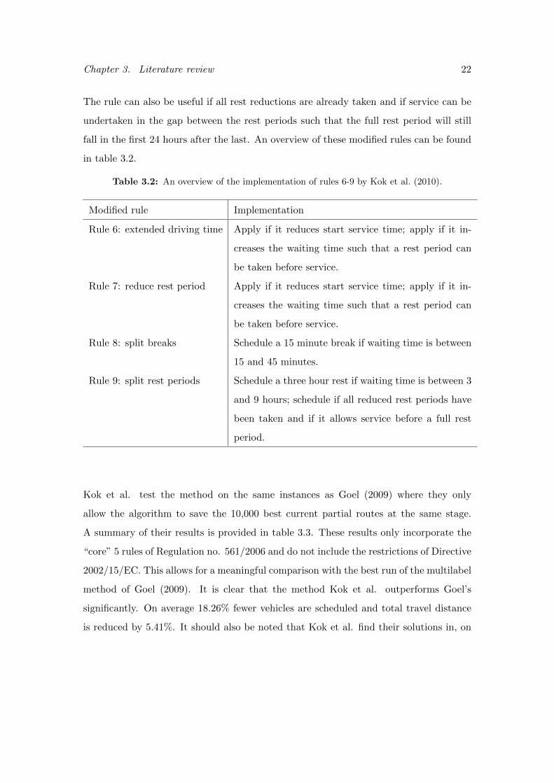
Chapter 3. Literature review 22
The rule can also be useful if all rest reductions are already taken and if service can be
undertaken in the gap between the rest periods such that the full rest period will still
fall in the first 24 hours after the last. An overview of these modified rules can be found
in table 3.2.
Table 3.2: An overview of the implementation of rules 6-9 by Kok et al. (2010).
Modified rule Implementation
Rule 6: extended driving time Apply if it reduces start service time; apply if it in-
creases the waiting time such that a rest period can
be taken before service.
Rule 7: reduce rest period Apply if it reduces start service time; apply if it in-
creases the waiting time such that a rest period can
be taken before service.
Rule 8: split breaks Schedule a 15 minute break if waiting time is between
15 and 45 minutes.
Rule 9: split rest periods Schedule a three hour rest if waiting time is between 3
and 9 hours; schedule if all reduced rest periods have
been taken and if it allows service before a full rest
period.
Kok et al. test the method on the same instances as Goel (2009) where they only
allow the algorithm to save the 10,000 best current partial routes at the same stage.
A summary of their results is provided in table 3.3. These results only incorporate the
“core” 5 rules of Regulation no. 561/2006 and do not include the restrictions of Directive
2002/15/EC. This allows for a meaningful comparison with the best run of the multilabel
method of Goel (2009). It is clear that the method Kok et al. outperforms Goel’s
significantly. On average 18.26% fewer vehicles are scheduled and total travel distance
is reduced by 5.41%. It should also be noted that Kok et al. find their solutions in, on
Chapter 3. Literature review 23
average, 67 seconds while Goel’s results are the best runs of five 30 minute runtimes.
Kok et al. indicate that this large improvement may be due to the flexibility of the
restricted dynamic programming approach in which the addition of complex constraints
such as driver regulations do not increase the runtime complexity of the algorithm. The
large neighbourhood search of Goel will however need more time to check for feasiblity
with the legislation and thus be able to investigate less neighbourhood solutions leading
to comparatively worse solutions.
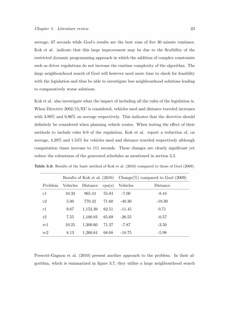
Kok et al. also investigate what the impact of including all the rules of the legislation is.
When Directive 2002/15/EC is considered, vehicles used and distance traveled increases
with 3.89% and 0.96% on average respectively. This indicates that the directive should
definitely be considered when planning vehicle routes. When testing the effect of their
methods to include rules 6-9 of the regulation, Kok et al. report a reduction of, on
average, 4.28% and 1.54% for vehicles used and distance traveled respectively although
computation times increase to 111 seconds. These changes are clearly significant yet
reduce the robustness of the generated schedules as mentioned in section 3.2.
Table 3.3: Results of the basic method of Kok et al. (2010) compared to those of Goel (2009).
Results of Kok et al. (2010) Change(%) compared to Goel (2009)
Problem Vehicles Distance cpu(s) Vehicles Distance
c1 10.33 965.44 55.04 -7.00 -8.44
c2 5.00 770.42 71.60 -40.30 -19.30
r1 9.67 1,152.39 62.51 -11.45 0.71
r2 7.55 1,100.83 65.69 -26.55 -0.57
rc1 10.25 1,300.60 71.27 -7.87 -3.50
rc2 8.13 1,266.64 68.68 -18.75 -5.98
Prescott-Gagnon et al. (2010) present another approach to the problem. In their al-
gorithm, which is summarized in figure 3.7, they utilize a large neighbourhood search

Chapter 3. Literature review 24
that chooses between different neighbourhood solutions to destroy parts of the current
solution and then uses a branch-and-price heuristic to reconstruct these parts. The
latter consists of solving a linear relaxation with column generation and afterwards a
branch-and-bound technique is used to generate integer solutions. To solve the column
generation subproblem, a tabu search heuristic is used that can delete a customer from
a route and insert another. Every time a customer is inserted into a route, a feasibil-
ity check needs to be performed which is rather simple for a VRPTW but gets more
complicated with driver rules.
Figure 3.7: The algorithm framework of Prescott-Gagnon et al. (2010).
The feasibility check is performed by use of an advanced labeling algorithm. Here, a

Chapter 3. Literature review 25
label represents a partial path that is feasible with all driver regulations (and of course
capacity and time window constraints). A label can be extended by investigating all
possible options of scheduling breaks and/or rests along the path to the next customer,
where only the feasible extensions will lead to new labels at the next customer. Prescott-
Gagnon et al., like Kok et al. (2010), test multiple cases of the regulations: with core
rules 1-5 of the regulation, with the rules of Directive 2002/15/EC and finally with rules
6-9 that are provisions on the core rules.
Prescott-Gagnon et al. (2010) were able to post results that were better than those from
Kok et al. (2010) and as far as we know, these are the current best solutions on the
instances introduced by Goel (2009). A comparison of the results on the complete set of
rules compared to Kok et al. can be seen in table 3.4. It is clear that Prescott-Gagnon
et al. dramatically improve the results, on average 13.4% less vehicles are scheduled and
13.2% less distance is traveled. The posted results are however the result of an average
of 5 runs of 88 minutes. When parameters are adjusted to only allow for a runtime of
one minute such as in the algorithm of Kok et al. (2010), the difference falls back to
7.5% less vehicles and 5.1% less distance traveled.
Table 3.4: Comparison of the results of Prescott-Gagnon et al. (2010) to those of Kok et al.
(2010) for the complete set of rules.
Results of Prescott-Gagnon
et al. (2010)
Change(%) compared to Kok
et al. (2010)
Problem Vehicles Distance cpu(min) Vehicles Distance
c1 10 847.61 88 -1 -9.6
c2 4.63 694.95 88 -11.8 -10.2
r1 8.08 975.91 88 -13.4 -14.6
r2 5.67 928.04 88 -22.9 -14.4
rc1 9 1,111.36 88 -10 -16
rc2 6.15 1,096.59 88 -24.4 -12.1
Chapter 3. Literature review 26
A final approach we consider in this section is provided by Goel (2010). Where all the
previous methods were integrated approaches where driver regulations are scheduled
during route generation, Goel presents a method which builds truck driver schedules
given a predetermined sequence of locations to visit. Furthermore, the approach guar-
antees to find a schedule complying with the regulation if such a schedule does exist,
which is not the case in the previous approaches. In order to do this, Goel improves on
his previous labeling approach (Goel, 2009). One of the main difficulties in scheduling
driver regulations is that it is often impossible to determine the best duration of rest
periods if not all future activities are known. It may prove necessary to extend the rest
period beyond the required 11 hours so that idle waiting time during the day is avoided
and no working time regulations are infringed. To tackle this difficulty, Goel schedules
normal rest periods and relaxes the constraint which states that a new rest period should
be taken in the 24 hours after the last. Once such a pseudofeasible schedule is found,
it can be made feasible by extending the previous rest period. Goel then presents a
method of myopically constructing driver schedules that adhere to this pseudofeasibil-
ity and imposes dominance criteria designed to reduce the number of partial schedules
needed to consider to solve the problem.
For the purpose of testing his approach, Goel generates 15.6 million instances feasible
with respect to time window constraints. Of these, only 662,308 were found to not exceed
the weekly driving and working times and only for 43,882 instances was it possible
to find a feasible schedule complying with the legislation. Goel also shows that the
previous approaches by Goel (2009) and Kok et al. (2010) construct feasible schedules
for much less instances. These methods are however much faster than the presented
approach, therefore Goel suggest limiting the search to only the most promising partial
schedules in each iteration. This does lower the amount of feasible schedules a bit but
still outperforms the previous approaches by a significant margin. An overview of the
results can be seen in table 3.5 where λ denotes the amount of customers in the instances.
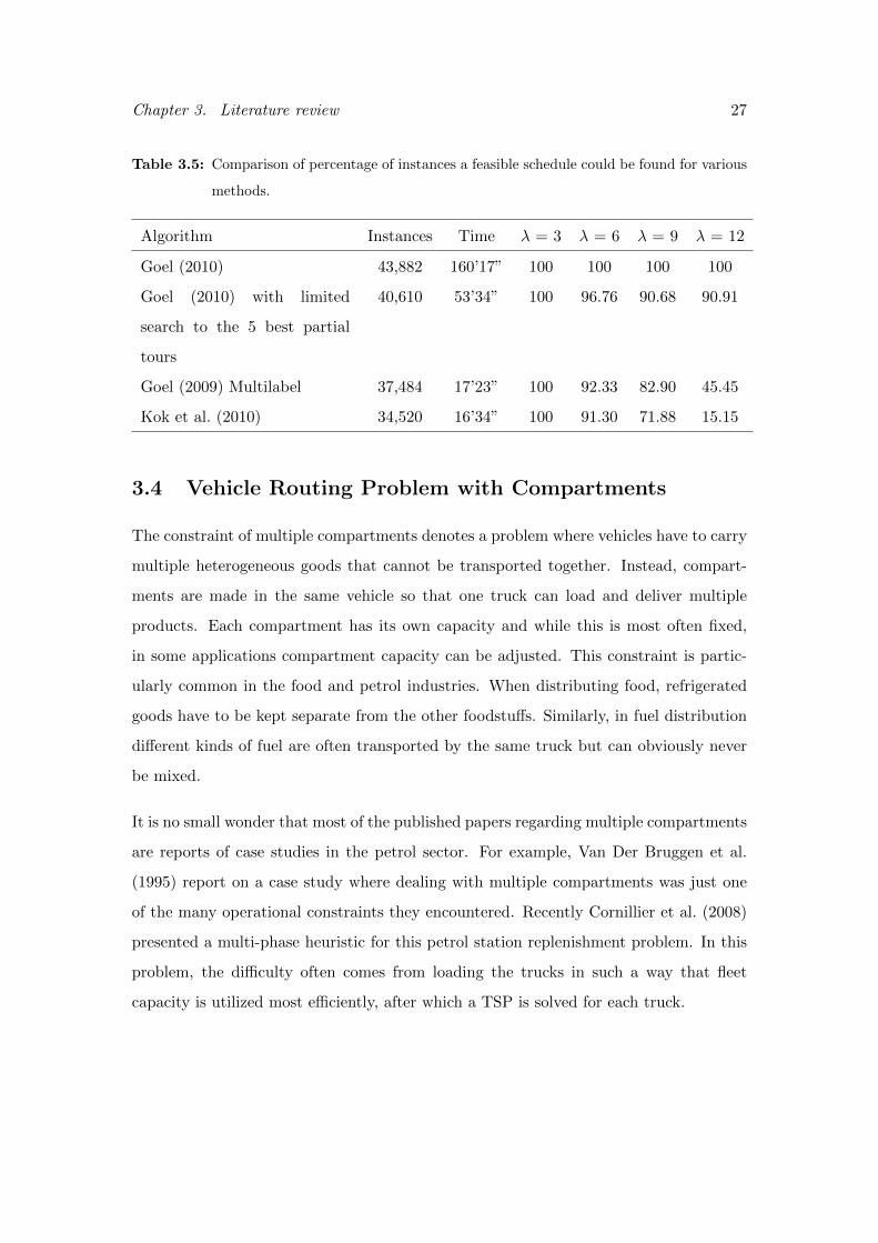
Chapter 3. Literature review 27
Table 3.5: Comparison of percentage of instances a feasible schedule could be found for various
methods.
Algorithm Instances Time λ = 3 λ = 6 λ = 9 λ = 12
Goel (2010) 43,882 160’17” 100 100 100 100
Goel (2010) with limited
search to the 5 best partial
tours
40,610 53’34” 100 96.76 90.68 90.91
Goel (2009) Multilabel 37,484 17’23” 100 92.33 82.90 45.45
Kok et al. (2010) 34,520 16’34” 100 91.30 71.88 15.15
3.4 Vehicle Routing Problem with Compartments
The constraint of multiple compartments denotes a problem where vehicles have to carry
multiple heterogeneous goods that cannot be transported together. Instead, compart-
ments are made in the same vehicle so that one truck can load and deliver multiple
products. Each compartment has its own capacity and while this is most often fixed,
in some applications compartment capacity can be adjusted. This constraint is partic-
ularly common in the food and petrol industries. When distributing food, refrigerated
goods have to be kept separate from the other foodstuffs. Similarly, in fuel distribution
different kinds of fuel are often transported by the same truck but can obviously never
be mixed.
It is no small wonder that most of the published papers regarding multiple compartments
are reports of case studies in the petrol sector. For example, Van Der Bruggen et al.
(1995) report on a case study where dealing with multiple compartments was just one
of the many operational constraints they encountered. Recently Cornillier et al. (2008)
presented a multi-phase heuristic for this petrol station replenishment problem. In this
problem, the difficulty often comes from loading the trucks in such a way that fleet
capacity is utilized most efficiently, after which a TSP is solved for each truck.

Chapter 3. Literature review 28
Fallahi et al. (2008) study a problem in which each compartment can only carry one
product in a broad sense, meaning that a product may represent a certain group of similar
goods. For example, food distribution often has trucks with a refrigerated compartment.
Furthermore, in this problem the different products do not have to be delivered at the
same time or by the same vehicle. This problem was dubbed the Multi-Compartment
Vehicle Routing Problem (MCVRP). Fallahi et al. (2008) propose several algorithms to
solve this problem, including a memetic algorithm and a tabu search. Since most of the
research regarding VRPs with compartments was based on case studies, the authors also
create instances based on known VRP instances.
Muyldermans and Pang (2010) concern themselves with the problem of waste collection
and investigate in which circumstances it can be useful to use waste collection trucks
with multiple compartments that can collect several different kind of waste at the same
time. They design a new local search procedure and compare their results with those of
Fallahi et al. (2008), they were able to report a slightly improved solution quality in less
computational time.
Derigs et al. (2010) provide another approach at the problem and develop an algorithm
comprising of several heuristics for the MCVRP. They present the notion of adding or
removing orders to a vehicle instead of customers and thus regard each order as separate
regardless of which customer it comes from. Where the previous approaches considered
a problem with two compartments and two orders per customer, Derigs et al. (2010) test
their implementation on new self-generated instances designed to resemble circumstances
in petrol and food distribution.
3.5 Contribution
Kok et al. (2010) suggested that the restricted dynamic programming approach is very
flexible and can be used to incorportate a variety of constraints with efficiency. In this
thesis, we will explore this suggestion and expand the VRPTWDR by incorporating

Chapter 3. Literature review 29
customers with demand for multiple products and trucks with multiple compartments.
Furthermore, although some work has been done regarding multiple compartments, no
effort has been made yet to include this constraint with time windows or other often
occuring operational constraints.
In this work, we aim to expand on the work of Kok et al. (2010) by using the restricted
dynamic programming to further incorporate more constraints in a rich VRPTW. We
also suggest a small improvement to the framework in the way it selects the most promis-
ing states.

Chapter 4
Solution Approach
Because the VRPTW has been studied so intensively, many heuristics have been pro-
posed to solve this problem and its various subproblems. In this chapter, we will elabo-
rate on one of these methods and explain how we have adapted it to account for both the
driver rules constraint and the multi compartment constraint. In section 4.1 we explain
the restricted dynamic programming approach while in section 4.2 and section 4.3 we
elaborate on how this approach is adapted.
4.1 Restricted Dynamic Programming
Restricted dynamic programming is a framework that finds its roots in the exact dynamic
programming algorithm of Held and Karp (1962) and Bellman (1962) designed for the
TSP where we consider a set V = {0, 1, . . . , n−1} of n nodes that each need to be visited
once in a way that total travel distance is minimized. A state (S, j), j ∈ S, S ⊆ V \0 in the
framework denotes a path starting at an original city 0 that visits all the customers in S
and ends at node j. The cost C(S, j) represents the cost of the path that minimizes travel
costs. When traveling from the depot, the costs are determined as C({j}, j) = c0j , ∀j ∈
V \0. In successive stages the recurrent relation C(S, j) = mini∈S\j{C(S\j, i) + cij} is
used until the optimal tour can be found in the last step by minj∈V \0{C(V \0, j) + cj0}.
30

Chapter 4. Solution Approach 31
In order to grasp these formulas, some explanation may be needed. When partial routes
are constructed, every state is expanded to every node the partial route has not visited
yet. This does not mean every new expanded partial route is kept in memory. For
example, sets {0, 1, 2} and {0, 2, 1} may both be expanded with node 3 which will lead
to two versions of the set S({0, 1, 2, 3}, 3) yet one will dominate the other because it
visited the nodes in a better order. In the dynamic programming approach, only the
path with minimal cost is saved and expanded in the next stage. Held and Karp (1962)
suggest a two-phase approach to calculate the optimal solution. In the first stage, all
costs C(S, j) are calculated according to the formulas above and at the end we know
the cost of the optimal solution. In the second phase, we determine the sequence of
nodes that allowed for this minimal cost by backtracking through the cost calculations
according to the following formula where (0i1i3 . . . in−1) is the optimal permutation.
C({i1, i2, . . . , ip, ip+1}, ip+1) = C({i1, i2, . . . , ip}, ip) + aipip+1 , for 1 ≤ p ≤ n− 2 (4.1)
This means that the last node is determined first and then successively the sequence of
nodes that make up for the optimal sequence until the first node is reached.
Since this algorithm was designed for the TSP, we need to find a way to apply it to the
VRP. Gromicho et al. (2009) presented the first application of the algorithm to the VRP
by using the giant-tour representation of Funke et al. (2005) to transform the VRP into
a sequencing problem. In this giant-tour representation each vehicle is designated an
origin and a destination node. In a VRP with one depot, these will always be in the
same location. A graphical interpretation can be seen in figure 4.1 where 4 routes are
divided over 2 depots. Here, every tour is ordered so that the destination node of the
first vehicle is immediately followed by the origin node of the second vehicle until the
destination of the last vehicle is linked with the first origin node. This way, a giant route
is created which converts the VRP into a sequencing problem like the TSP and allows
the dynamic programming method to be used. In the VRP however, special attention
needs to be given to the feasibility of expansions. This means that a new vehicle can
only start his route after the previous vehicle has returned to the depot. Furthermore,

Chapter 4. Solution Approach 32
each expansion needs to be feasible regarding capacity, time window and in our case
driver rules and compartment constraints.
Figure 4.1: Giant-tour representation by Funke et al. (2005).
Given the complexity of VRPTW, exact algorithms are not fast enough to solve problems
of realistic size. This is not different for the dynamic programming approach. Malandraki
and Dial (1996) therefore introduced the idea of restricting this algorithm. They define
the parameter H which defines the maximum amount of partial routes that are expanded
in the next stage. Of course we will only expand the H most promising states. This
allows the user to choose a computational complexity somewhere between the nearest-
neighbour heuristic (with H = 1) and the exact algorithm (with H =∞). Selecting the
H most promising states comes down to what the user defines as “promising”. In our
implementation this means only the states with the lowest cost are preserved where cost
denotes the amount of vehicles used, distance traveled so far and how far the vehicle is in
its workweek. The computational complexity can be further reduced by only considering
the E nearest unvisited nodes for expansion. We do check for feasibility of each expansion
and only the feasible ones are maintained. Both these restrictions imply that it is not
guaranteed that the optimal solution is found but partial routes with low costs will
probably lead to better solutions than those with higher costs.
Gromicho et al. (2009) suggested that the restricted dynamic programming framework
is a very flexible approach and can be used to incorporate many operational constraints
efficiently. This can be done by adding state dimensions to each partial tour. Thus,

Chapter 4. Solution Approach 33
a state represents the path followed by the partial route so far, the distance it has
traveled, the amount of vehicles that are used and any dimensions needed for operational
constraints. For example, to solve the VRPTW, two state dimensions are added. The
first denotes the remaining capacity of the current vehicle while the second stands for
the departure time at the last customer. This allows us to check for feasibility at each
expansion of a state.
Gromicho et al. (2009) tested this approach and came to the conclusion that although the
algorithm cannot compete with state of the art local search techniques for the VRPTW,
it can be used with success in rich VRP since the dynamic programming algorithm does
not increase in runtime complexity if extra state dimensions are added. Indeed, Kok
et al. (2010) were able to publish promising results when they applied the framework to
the VRPTW with driver rules.
4.2 Break and Rest Scheduling
In order to include the EU legislation in the restriced dynamic programming approach,
we add multiple new state dimensions. In this section we explain the break schedul-
ing method of Kok et al. (2010) and show how this fits into the dynamic programming
method. Kok et al. (2010) argue for an algorithm that decides locally how to plan breaks
and rest periods. A first benefit is that this does not increase the complexity of the algo-
rithm as breaks and rest periods can be scheduled in constant time. Furthermore, this
ensures that the rules presented here are relatively easy to understand and implement.
In this scheduling method, we make a small simplification in that after no more than six
hours of working time, a break of 45 minutes is scheduled instead of the required 30 min
as postulated by Directive 2002/15/EC. This means that the break requirement is also
satisfied if the work day exceeds nine hours and that any working break will also count
as a break from driving.
We use six extra state dimensions that keep track of the various working and driving

Chapter 4. Solution Approach 34
periods and allow us to notice when it is necessary to schedule a break or rest. These
dimensions are summarized in table 4.1. In addition, this scheduling method will only
consider a planning horizon of one week and starts right after the weekend which means
that all the mentioned state dimensions start at zero.
Table 4.1: State dimensions used by Kok et al. (2010) to schedule breaks and rests.
tnbw Nonbreak working time, which is the total amount of working time since the
last break of 45 minutes or more.
tnbd Nonbreak driving time, which is the total amount of driving time since the
last break of 45 minutes or more.
tnr Nonrest time, which is the total amount of time since the last rest period of
11 hours or more.
tdd Daily driving time, which is the total amount of driving time since the last
rest period of 11 hours or more.
tww Weekly working time, which is the total amount of working time since the
weekend (rest period of at least 45 hours).
twd Weekly driving time, which is the total amount of driving time since the
weekend (rest period of at least 45 hours).
Before any breaks or rest periods are considered, we verify if the vehicle can actually
return to the depot after it travels to the customer. This can be prohibited by the weekly
working and driving time. Therefore, if we consider dij as the driving time between node
i and j and sj as the service time of customer j, no expansion is made if one or more of
the following statements are false.
dij + dj0 ≤ 56− twd (4.2)
dij + sj + dj0 ≤ 60− tww (4.3)
When starting to expand a state (S, i) to another node j, we have to calculate the arrival
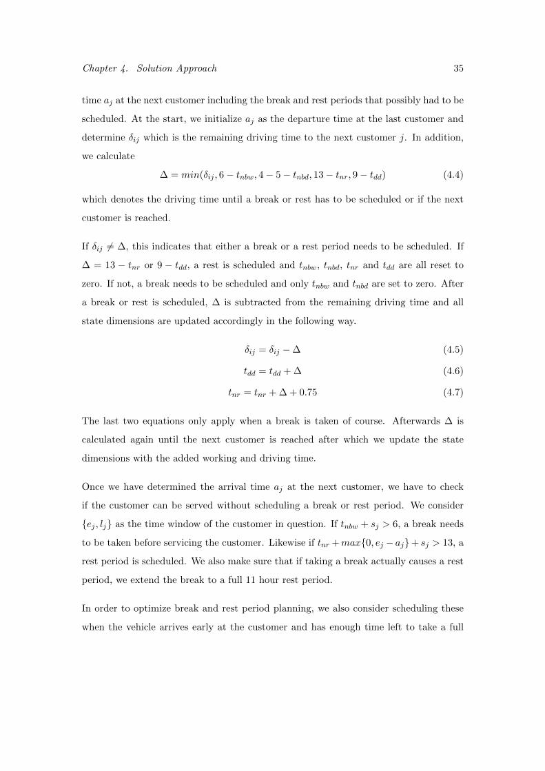
Chapter 4. Solution Approach 35
time aj at the next customer including the break and rest periods that possibly had to be
scheduled. At the start, we initialize aj as the departure time at the last customer and
determine δij which is the remaining driving time to the next customer j. In addition,
we calculate
∆ = min(δij , 6− tnbw, 4− 5− tnbd, 13− tnr, 9− tdd) (4.4)
which denotes the driving time until a break or rest has to be scheduled or if the next
customer is reached.
If δij 6= ∆, this indicates that either a break or a rest period needs to be scheduled. If
∆ = 13 − tnr or 9 − tdd, a rest is scheduled and tnbw, tnbd, tnr and tdd are all reset to
zero. If not, a break needs to be scheduled and only tnbw and tnbd are set to zero. After
a break or rest is scheduled, ∆ is subtracted from the remaining driving time and all
state dimensions are updated accordingly in the following way.
δij = δij −∆ (4.5)
tdd = tdd + ∆ (4.6)
tnr = tnr + ∆ + 0.75 (4.7)
The last two equations only apply when a break is taken of course. Afterwards ∆ is
calculated again until the next customer is reached after which we update the state
dimensions with the added working and driving time.
Once we have determined the arrival time aj at the next customer, we have to check
if the customer can be served without scheduling a break or rest period. We consider
{ej , lj} as the time window of the customer in question. If tnbw + sj > 6, a break needs
to be taken before servicing the customer. Likewise if tnr +max{0, ej − aj}+ sj > 13, a
rest period is scheduled. We also make sure that if taking a break actually causes a rest
period, we extend the break to a full 11 hour rest period.
In order to optimize break and rest period planning, we also consider scheduling these
when the vehicle arrives early at the customer and has enough time left to take a full

Chapter 4. Solution Approach 36
rest period or break. These are then extended until the start of the time window such
that as many of the state dimensions of table 4.1 as possible are set to zero when service
finally starts. Furthermore, if the waiting time between the arrival at the customer and
the start of the time window is insufficient to schedule a rest period but if a rest is taken
along the way, this rest period is extended in such a way that the vehicle will arrive at
the customer at the start of the time window.
If a short waiting time is still needed before the time window opens, we increase tnr and
tnbw with the waiting time. Finally, we verify that the arrival time aj does not exceed
the due date lj so we do not violate the time window. Only then is the state expanded
and evaluated in regards to cost to see if the expand state belongs to the best H states.
4.3 Multiple Compartments Method
As Gromicho et al. (2009) have pointed out, the restricted dynamic programming ap-
proach is a very flexible approach and it can handle many operational constraints with
ease. In this section we will explain how to incorporate multiple compartments into
the method. We will explore a problem in which each vehicle has two compartments
and each customer has a demand for two separate products. As Fallahi et al. (2008)
mentioned, it makes sense to limit ourselves to two products and compartments because
of the following reasons.
� It corresponds with the often-used example of food distribution with a freezing
compartment.
� This allows for an easier comparison with solutions of just one product.
� In many short haul instances, dividing original customers demands into three or
more products makes these demands marginal.
� With two compartments, the VRP already gets much more complex and it is
difficult enough to show our approach.

Chapter 4. Solution Approach 37
A first step is to replace the state dimension of remaining capacity of the current vehicle
by two new state dimensions which denote the remaining capacity of compartment A
and compartment B. Compartment A is used to transport product A and compartment
B to transport product B. These products can never be in the same compartment and
product A can never be stored in compartment B, likewise for product B. The demand
for the different products at the customers is determined in a semi-random way and the
capacity of the two compartments is defined by the fractions each product represents
in the total demand. Note that if every customer had a demand in the same ratio as
the compartment capacities, this would lead to the identical solution of the VRP with
one compartment and one product. Service time for each product is for simplicity’s sake
equal to half of the original service time for one product.
We take the suggestion of Derigs et al. (2010) by heart and treat each order separately.
As a consequence, this means that for the same amount of customers we now double the
amount of times every state is expanded. We ensure that the vehicle only returns to the
depot when both remaining capacities are insufficient to service either of the demands
at the customer to be expanded towards. When both demands still need to be fulfilled
at a target customer, the customer is serviced first for product A. We are sure every
demand will be fulfilled when the algorithm starts since every customer with at least
one demand yet to be delivered is considered for expansion at every stage. This also
means that since the algorithm only keeps the states with lowest cost, expansions to the
other order at the same customer (if enough capacity remains to fulfill the demand for
the other product) will be prioritized since no extra cost will be incurred this way.
When demand for product A at the current location is already serviced while this is
not the case for product B and if enough capacity remains in compartment B to service
demand for product B, we only consider expansion to the order for product B at the
same customer instead of expanding to all other customers with unserviced orders. This
significantly reduces the computational complexity.

Chapter 4. Solution Approach 38
In some cases, it may be required by the customers to service both demands at the same
time by the same vehicle. This can be done by only considering expansion to customers
for which the current vehicle has enough capacity to service both demands. Of course,
this will deteriorate the solution quality since in many cases vehicles will have to return
to the depot even though enough capacity remains in one of the two compartments.
This method also allows for an easy integration with the break scheduling method de-
scribed in section 4.2. Whenever we expand to a next order, the break scheduling method
is run and the needed breaks and rest periods are planned in the same way as with the
VRP with one compartment. When the expansion is made to the order for the other
product at the same customer, δij will be zero and no rest or break periods can be
planned.
Chapter 5
Computational Results
In this chapter we will present our computational results done on various experiments
with the restricted dynamic programming approach. First we will test the method on
the regular VRPTW in order to create a benchmark of results so we can investigate the
effect of the constraints considered in this thesis. Second we will post results on including
driver rules and multiple compartments and elaborate on the impact of these constraints
and of our method of implementing them. Finally, we combine the constraints into one
model and see how this affects the quality of our solutions.
All the tests are done on the instances proposed by Solomon (1987) although they are
slightly modified to make sure they are meaningful instances to test our constraints
on. The Solomon instances consist of 56 instances with 100 customers each. Each
customer has its own coordinates in a 2d plane around the depot and possesses a certain
demand, time window and service time. There are 6 categories to be discerned: the c1
and c2 categories make for clustered customers while the r1 and r2 categories represent
customers with random locations. The rc1 and rc2 instances provide a middle ground.
The 1-instances are designed to resemble short haul problems where vehicles have a
relatively small capacity and time horizon, while the 2-instances resemble long haul
problems with large capacities and a large time horizon. All tests were programmed in
C++ and were run on a Core 2 Duo E8500 processor clocked at 3.16Ghz although the
39
Chapter 5. Computational Results 40
program was not optimized for multi-core processing.
5.1 Restricted Dynamic Programming for the VRPTW
As Gromicho et al. (2009) indicated, the restricted dynamic programming approach
cannot compete with top local search methods for the VRPTW. With an H of 100,000
they report 1.27 more vehicles and 11% more distance traveled on average. In this
section we will post results on the modified instances by Goel (2009) in order to create
a set of results to which we can benchmark our results including the driver rules and
multiple compartments constraints.
Goel (2009) suggested to rescale the depot opening times to 144 hours as this is the
maximum of one workweek in the EU legislation. All the time windows of the customers
are rescaled accordingly. The driving speed is fixed at 5 distance units per hour and
service time is one hour for every customer. Because of required breaks and rest, it
may become impossible to reach certain customers before their due date or return to
the depot after starting service at their ready time. As a result, time windows of these
customers are adjusted in such a way that the ready time is equal to the earliest time a
vehicle can reach the customer while the due date is set so that starting service at this
time and returning directly to the depot results in a return time at the depot’s due date.
In our experiments, the maximum number of states to be taken to the next iteration H
is set to 10,000 which allows for a computation time under one minute for every instance
while E, the amount of unvisited nodes to be taken into consideration, is left unlimited.
The most promising states are selected using the following hierarchy. The number of
vehicles is the primary objective with the total distance traveled as second and elapsed
time as a final objective. This last objective prevents that partial tours that score low
on the first two objectives yet have tens of waiting hours will be preferred over states
with a similar vehicle and distance count but with a higher time-effiency. This hierarchy
is achieved by adding a large number (100) to the cost every time a vehicle returns to

Chapter 5. Computational Results 41
the depot while distance is added with a factor one and time elapsed with a factor of
0.5.
Table 5.1 summarizes our results for the VRPTW without driver rules or multiple com-
partment constraints. For the sake of readability, in this chapter all tables will present
averages per category of instances. For results per individual instance, we refer to ap-
pendix B.
Table 5.1: Results for the VRPTW.
Problem Distance Vehicles cpu(s)
c1 1098.04 10 25.9
c2 734.43 3.25 19.6
r1 1256.86 8.08 24.7
r2 1197.74 4.36 18.5
rc1 1438.38 9.13 23.5
rc2 1386.01 5 17.3
5.2 Driver Rules
Table 5.2 visualizes the results when we include the break scheduling method as described
in section 4.2. On average the distance traveled stays the same (-0.7%) yet on average
36% more vehicles are used. Especially in the long haul instances, we notice a remarkable
increase. This is quite logical as taking extra break and rest periods will not necessarily
increase distance traveled yet will force each vehicle to serve less customers on their tour.
The results indicate that driver regulations have a very large impact and should definitely
be included in any real life routing solution. Although computation time does increase
with 41.3%, it is clear that these times are still very fast and practically acceptable.
When our solutions are compared to those of Kok et al. (2010) we schedule 4.7% less

Chapter 5. Computational Results 42
vehicles yet incur 5.7% more distance traveled. This difference can be explained partially
by some small differences in implementation but most importantly by taking elapsed
time into account when determining the most promising states while Kok only considers
the amount of vehicles and distance traveled. These results indicate that the method
of determining the most promising states is extremely important in the generation of
quality solutions.
A peculiar effect can be noticed in some c1 instances where adding driver rules actually
improves the solution. It seems that the driver regulation constraints in some cases help
to restrict the search space and choose the most promising states.
Table 5.2: Results when including driver regulations compared to those of the standard
VRPTW.
VRPTWDR Change (%)
Problem Distance Vehicles cpu(s) Distance Vehicles cpu(s)
c1 1040.61 10.11 30.33 -5.3 1.1 17.1
c2 842.14 5.5 28.25 14.7 69.2 44.1
r1 1245.70 9.25 32 -0.8 14.5 29.6
r2 1138.47 7.09 30 -4.9 62.6 62.2
rc1 1410.53 10.13 30.38 -1.9 11 29.3
rc2 1302.04 7.88 28.63 -6.1 57.6 65.5
5.3 Multiple Compartments
Before we are able to test our approach, we need to modify our instances in such a way
that two capacities and two orders per customer are present. The research community
has generated instances but these never include time windows at the customer. Since
we want to include time windows in our tests and want to generate results that allow
us to compare results with the general case in a meaningful way, we opt to change the

Chapter 5. Computational Results 43
modified solomon instances by Goel (2009) slightly.
We will modify these instances in the same way as Fallahi et al. (2008). Every customer
is randomly divided into two parts. For each customer i, the demand for product A can
be calculated as qiA = qi/k with k a random integer in [3, 5] and qi the original demand
of the customer. The demand for product B logically is qiB = qi − qiA. To determine
the capacities of the two compartments, we sum up all the customers for product A and
B and calculate their averages. Capacity for compartment A can then be determined as
QA = (Q ∗ qA)/(qA + qB) and capacity for compartment B as QB = Q − QA where Q
stands for capacity and q is average demand.
Table 5.3 shows the results for the first case in which the two different orders of a
customer can be delivered by different vehicles at different times (although still within
the time window). On average we need 3.6% more vehicles and 5.7% more distance needs
to be travelled in order to cope with the random demands. Note that if no randomness
was present in splitting up the demand, we would achieve the same results as for the
“regular” VRPTW. Since we have to expand order per order instead of per customer,
complexity is significantly increased with 76% more needed runtime on average.
Table 5.3: Results of the VRPTW with multiple compartments compared to the regular
VRPTW results.
VRPTW-MC Change (%)
Problem Distance Vehicles cpu(s) Distance Vehicles cpu(s)
c1 1261.25 10.33 46.5 14.9 3.3 79.5
c2 720.44 3.38 32.63 -1.9 4 66.5
r1 1427.28 8.75 49.7 13.6 8.3 101.2
r2 1207.53 4.27 30.27 0.8 -2 63.6
rc1 1550.76 9.38 43 7.8 2.7 83
rc2 1373.08 5.25 28.5 -0.9 5 64.7

Chapter 5. Computational Results 44
We also investigate the case in which delivery of the two orders has to happen with one
vehicle. We notice remarkable results in table 5.4 as we need 3.1% less vehicles and need
to travel 4.2% less distance compared to the multiple delivery problem. Even more,
this decreases the extra computational effort needed from 76% to 59% compared to the
standard VRPTW case.
Since both deliveries have to comply with one time window, it often makes sense to
deliver the two products at the same time. As such it is not suprising that joint delivery
leads to better solutions yet the first method should have been able to detect this and
come up with the same solutions as in the joint delivery problem. This seems to indicate
that our current method of selecting the most promising states is too myopic.
Table 5.4: Results of the VRPTW with multiple compartments and one delivery compared to
the case with multiple deliveries.
VRPTW-MC Joint Delivery Change (%)
Problem Distance Vehicles cpu(s) Distance Vehicles cpu(s)
c1 1199.42 10.44 41.1 -4.9 1.1 -11.6
c2 714 3.13 30.63 -0.9 -7.4 -6.1
r1 1304.27 8.7 38.7 -8.6 -0.1 -22.1
r2 1183.64 4.09 29.5 -2 -4.2 -2.5
rc1 1461.07 9.75 37.6 -5.8 3.9 -12.6
rc2 1335.99 4.63 28.38 -2.7 -11.8 0
5.4 Multiple Compartments and Driver Rules
As we mentioned in section 4.3, the restricted dynamic programming approach allows for
an easy implementation and integration of various constraints. In this section, we will
showcase that characteristic by combining previous constraints of driver rules and mul-
tiple compartments into one whole. Since the last section indicated better results when

Chapter 5. Computational Results 45
the two orders were delivered at the same time, we will continue with that particular
implementation.
In table 5.5, we notice a similar effect as in section 5.2 where the traveled distance
stays constant yet the amount of vehicles needed increases dramatically with 30.4%.
Computational times increase with 35.1% which is consistent with the case without
multiple compartments.
Table 5.5: Results of all constraints combined compared to the case with only multiple com-
partments.
VRPTW-MC with Driver Rules Change (%)
Problem Distance Vehicles cpu(s) Distance Vehicles cpu(s)
c1 1169.28 10.67 50.67 -2.5 2.2 23.2
c2 792.75 4.63 44.38 11 47.9 44.9
r1 1250.12 9.33 49.67 -4.2 7.2 28.3
r2 1165.59 6.09 43.27 -1.5 48.9 46.7
rc1 1431.57 10 45 -2 2.6 19.7
rc2 1308.16 7.25 42 -2.1 56.6 48

Chapter 6
Conclusion
In this work we discuss the Vehicle Routing Problem (VRP) and some common opera-
tional constraints associated with this problem. In a VRP the objective is to service a
set of customers, each with a designated demand, from one or more central depots with
a minimal set of vehicles and with minimal distance traveled by all vehicles.
Many operational constraints have to be considered when designing routes in real life
problems. We will limit ourselves to discuss time windows, driver legislation and multiple
compartments. In a VRP with time windows, the service for each customer has to start
within a certain time span. Furthermore, in practical cases each route has to comply with
EU legislation regarding break and rest periods for drivers, else the company responsible
will be held accountable for infringing these rules. As a last case, we consider the case
where vehicles have to deliver multiple products that cannot be transported in the same
vehicle compartment, thus multiple compartments within the vehicle are needed. This
is common in industries like food and petrol distribution and is becoming more relevant
in other industries due to increased use of horizontal collaboration within the supply
chain.
While scientific research on the topic of time windows has been plentiful, very little at-
tention has been given to the lesser known constraints. Both driver rules and multiple
compartments have a large impact on the feasibility of constructed tours. It is therefore
46

Chapter 6. Conclusion 47
of prime importance to develop methods that efficiently check feasibility whenever cus-
tomers are inserted or added to a tour. In this thesis, we expand on a recently suggested
approach which is new to the VRP altogether.
Restricted dynamic programming is a construction heuristic based on the exact dynamic
programming approach used on the Traveling Salesman Problem (TSP). In the exact
approach, we construct partial routes (or states) and expand all routes with all nodes
yet unvisited. Since this would lead to unacceptable runtimes, we restrict the approach
to only expand to a certain user specified amount of the most promising states. The
approach has proven to be very successful in dealing with rich VRPs (VRPs with many
constraints) as new constraints can easily be added via state dimensions which keep
track of many constraint variables during route construction.
We provide results on various combinations of constraints on the VRP which indicate
that the restricted dynamic approach indeed is able to quickly find quality solutions with
relatively little extra computational time needed. When we consider driver rules, it is
shown that especially in the long haul cases these rules have a very large impact and
should be directly considered when planning routes. Considering multiple compartments,
we have modified existing instances and were able to come to solutions in the two product
case which only required 60 to 70% more computation time. As a showcase of the
flexibility of the approach, we incorporate driver rules into the multiple compartment
subproblem and come to the same conclusion as when incorporating these rules into the
standard VRPTW.
Naturally, our research has its limits. The results we obtained seem to indicate that the
approach is very susceptible to the way how one selects the most promising states at
every stage of construction. While we have provided some efforts by including elapsed
time in this method, it is clear that further research into this topic can be very revealing
and could help to improve solutions obtained by this method.
Some discussion exists within the research community whether some provisional rules

Chapter 6. Conclusion 48
of the EU legislation should be taken into account at the vehicle routing stage. Results
indicate that if this is done, solution quality increases by a small amount yet one may
also argue that this inclusion will reduce robustness of the obtained results and will be
of low value in practice. It would be very interesting to study this effect on real life data
and discover how important these provisions are in practice.
Finally, while we have discussed some operational constraints, there are often many
more in a practical scenario. Kok (2010) provides an example with traffic congestion in
his doctoral thesis. It could be an interesting topic to further explore the possibilities
of the restricted dynamic programming framework on many other common operational
constraints such as time-dependent travel times, multiple depots, etc.

Appendix A
Pseudo Code
In this section we will provide some details on the implementation of the restricted
dynamic programming algorithm. Before a brief pseudo code overview is given, we
raise the attention to data structures. Since the framework relies on being able to
recognize and store the H most promising states, the choice of data structure is crucial
for performance. It should be able to have fast access to both the absolute most promising
state stored so far (the one with the least cost) and it should be able to quickly identify
the worst solution stored so far so it can be compared to new expansions. If new
expansions have a lower cost value, the worst stored state should be replaced by the new
expansion.
We have chosen to implement this via a so-called min-max heap introduced by Atkinson
et al. (1986). This is a heap structure in which the rows of the heap consist of alter-
natively minimum and maximum values. This means that at the top of the heap the
minimum value is stored and on the second row the maximum value. This allows for
to find both the minimum and maximum value stored in constant time while insertions
and deletions happen in logarithmic time (because the heap structure needs to be up-
dated every time this happens). Atkinson et al. (1986) provided clear pseudo code to
help programmers in the implementation, as such no such code will be present in this
appendix. Once all states are expanded, the final best H states are copied to a normal
49

Appendix A. Pseudo Code 50
vector for storage.
A.1 Basic Method for the VRPTW
Define vector
for all stages do
Create heap
for Every state do
for Every unvisited node do
if capacity ¡ customer demand then
return to depot
else
BREAK SCHEDULING METHOD
calculate distance and travel time
if Arrival time > due date customer then
STOP
end if
if Heap has free space available then
Expand state with unvisited node
Insert state into the heap
else
if (cost of state + distance to unvisited node) < cost of maximum value
in heap then
Expand state with unvisited node
Delete maximum from the heap
Insert state into the heap
end if
end if
end if

Appendix A. Pseudo Code 51
end for
end for
vector ← heap
end for
A.2 Break and Rest Scheduling Method
This pseudo code is put in place of BREAK SCHEDULING METHOD in the previous
section. Since Kok et al. (2010) already provided pseudo code regarding the break
scheduling method, we refer the reader to that paper.
A.3 Multiple Compartments
We first consider the alternative where orders from the same customer are allowed to be
delivered by different vehicles.
Define vector
for all stages(200 orders) do
Create heap
for Every state do
if product A is delivered at current position and product B has not been delivered
yet and capacityB ¿ demandB then
expand state only with order for product B
end if
for Every node with at least one product yet to be delivered do
if capacityA ¡ demandA and capacityB ¡ demandB then
return to depot
else
BREAK SCHEDULING METHOD
calculate distance and travel time
if Arrival time > due date customer then
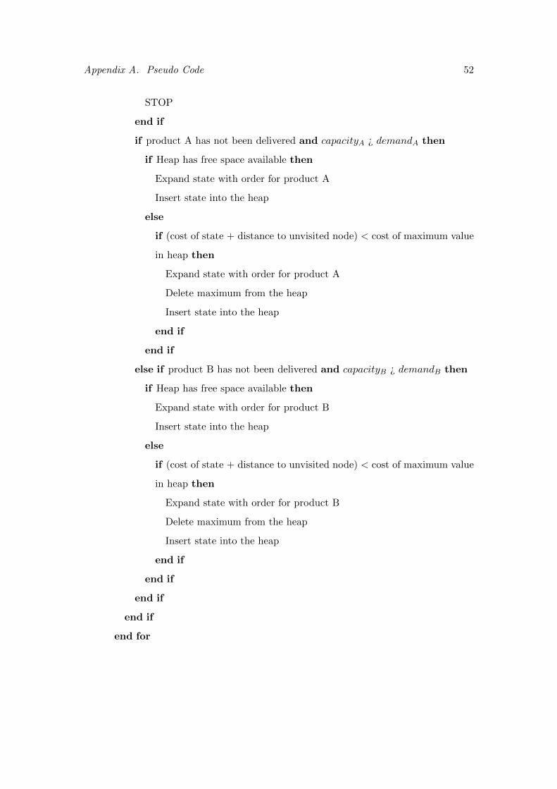
Appendix A. Pseudo Code 52
STOP
end if
if product A has not been delivered and capacityA ¿ demandA then
if Heap has free space available then
Expand state with order for product A
Insert state into the heap
else
if (cost of state + distance to unvisited node) < cost of maximum value
in heap then
Expand state with order for product A
Delete maximum from the heap
Insert state into the heap
end if
end if
else if product B has not been delivered and capacityB ¿ demandB then
if Heap has free space available then
Expand state with order for product B
Insert state into the heap
else
if (cost of state + distance to unvisited node) < cost of maximum value
in heap then
Expand state with order for product B
Delete maximum from the heap
Insert state into the heap
end if
end if
end if
end if
end for

Appendix A. Pseudo Code 53
end for
vector ← heap
end for
The following code presents the needed adjustments so every customer has a joint de-
livery of both products by the same vehicle.
Define vector
for all stages(200 orders) do
Create heap
for Every state do
for Every node with both product yet to be delivered do
if capacityA ¡ demandA or capacityB ¡ demandB then
return to depot
else
BREAK SCHEDULING METHOD
calculate distance and travel time
if Arrival time > due date customer then
STOP
end if
if product A has not been delivered and capacityA ¿ demandA and product
B has not been delivered and capacityB ¿ demandB then
if Heap has free space available then
Expand state with order for product A
Expand state with order for product B
Insert state into the heap
else
if (cost of state + distance to unvisited node) < cost of maximum value
in heap then
Expand state with order for product A
Expand state with order for product B
Appendix A. Pseudo Code 54
Delete maximum from the heap
Insert state into the heap
end if
end if
end if
end if
end for
end for
vector ← heap
end for
Appendix B
Detailed Computational Results
In the following tables the full results for five experiments are posted: the standard
VRPTW, the VRPTW with driver rules, the VRPTW with multiple compartments
(separate deliveries), the VRPTW with multiple compartments (joint deliveries) and
finally the VRPTW with multiple compartments (joint deliveries) and driver rules.
55

Appendix B. Detailed Computational Results 56
Table B.1: Results for the standard VRPTW.
Problem Distance Vehicles cpu(s) Problem Distance Vehicles cpu(s)
c101 968.49 10 21 c201 625.31 3 22
c102 1157.43 10 29 c202 688.87 3 19
c103 1214.93 10 32 c203 761.9 4 19
c104 1293.45 10 19 c204 1026.09 4 19
c105 1016.1 10 23 c205 636.94 3 21
c106 1003.01 10 26 c206 725.39 3 20
c107 1065.14 10 25 c207 760.11 3 18
c108 1044.21 10 29 c208 650.8 3 19
c109 1119.57 10 29
c1 1098.04 10 25.9 c2 734.43 3.25 19.6
r101 1603.78 8 27 r201 1536.09 6 21
r102 1408.83 9 30 r202 1434.23 5 23
r103 1250.67 8 27 r203 1183.62 5 21
r104 1146.96 8 21 r204 1057.63 4 18
r105 1352.49 8 29 r205 1354.58 4 18
r106 1303.12 8 30 r206 1187.44 4 20
r107 1228 8 24 r207 1089.71 4 18
r108 1111.53 8 21 r208 939.28 3 17
r109 1189.38 8 23 r209 1132.55 4 17
r110 1149.05 8 21 r210 1253.32 5 17
r111 1186.32 8 25 r211 1006.65 4 14
r112 1152.22 8 18
r1 1256.86 8.08 27.7 r2 1197.74 4.36 18.6
rc101 1545.37 10 24 rc201 1719.71 7 18
rc102 1540.38 9 26 rc202 1561.33 5 20
rc103 1382.67 9 26 rc203 1319.23 5 18
rc104 1400.25 9 19 rc204 1090.9 4 17
rc105 1611.51 9 25 rc205 1613.28 6 18
rc106 1394.68 9 25 rc206 1288.15 5 17
rc107 1343.36 9 24 rc207 1358.17 4 16
rc108 1288.82 9 19 rc208 1137.27 4 14
rc1 1438.38 9.125 23.5 rc2 1386 5 17.25
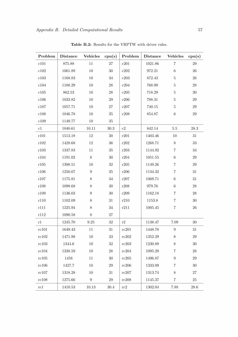
Appendix B. Detailed Computational Results 57
Table B.2: Results for the VRPTW with driver rules.
Problem Distance Vehicles cpu(s) Problem Distance Vehicles cpu(s)
c101 875.88 11 27 c201 1021.86 7 29
c102 1061.89 10 30 c202 972.21 6 26
c103 1168.83 10 34 c203 872.43 5 26
c104 1108.29 10 28 c204 768.99 5 28
c105 862.53 10 28 c205 718.29 5 30
c106 1033.82 10 29 c206 788.31 5 29
c107 1057.71 10 27 c207 740.15 5 29
c108 1046.78 10 35 c208 854.87 6 29
c109 1149.77 10 35
c1 1040.61 10.11 30.3 c2 842.14 5.5 28.3
r101 1513.18 12 30 r201 1403.46 10 31
r102 1428.68 12 36 r202 1268.71 8 33
r103 1337.83 11 35 r203 1144.92 7 34
r104 1191.02 8 30 r204 1051.55 6 29
r105 1398.51 10 32 r205 1149.26 7 29
r106 1250.07 9 35 r206 1134.32 7 31
r107 1175.81 8 34 r207 1069.71 6 31
r108 1098.68 8 30 r208 979.76 6 28
r109 1136.03 9 30 r209 1162.18 7 28
r110 1102.09 8 31 r210 1153.8 7 30
r111 1225.94 8 34 r211 1005.45 7 26
r112 1090.58 8 27
r1 1245.70 9.25 32 r2 1138.47 7.09 30
rc101 1649.43 11 31 rc201 1448.78 9 31
rc102 1471.98 10 33 rc202 1352.29 8 29
rc103 1344.6 10 32 rc203 1230.89 8 30
rc104 1338.59 10 28 rc204 1095.29 7 28
rc105 1458 11 30 rc205 1496.87 9 29
rc106 1427.7 10 29 rc206 1333.09 7 30
rc107 1318.28 10 31 rc207 1313.74 8 27
rc108 1275.66 9 29 rc208 1145.37 7 25
rc1 1410.53 10.13 30.4 rc2 1302.04 7.88 28.6
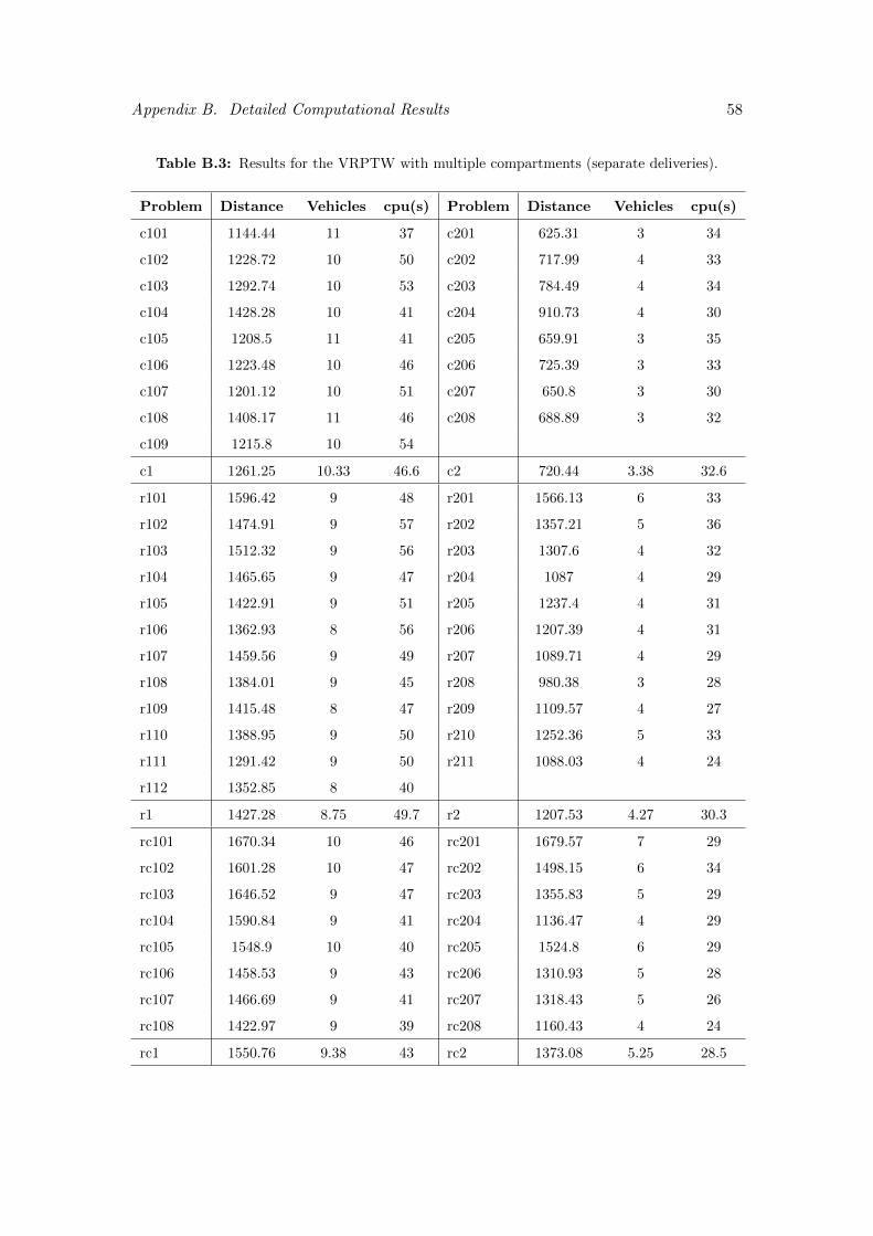
Appendix B. Detailed Computational Results 58
Table B.3: Results for the VRPTW with multiple compartments (separate deliveries).
Problem Distance Vehicles cpu(s) Problem Distance Vehicles cpu(s)
c101 1144.44 11 37 c201 625.31 3 34
c102 1228.72 10 50 c202 717.99 4 33
c103 1292.74 10 53 c203 784.49 4 34
c104 1428.28 10 41 c204 910.73 4 30
c105 1208.5 11 41 c205 659.91 3 35
c106 1223.48 10 46 c206 725.39 3 33
c107 1201.12 10 51 c207 650.8 3 30
c108 1408.17 11 46 c208 688.89 3 32
c109 1215.8 10 54
c1 1261.25 10.33 46.6 c2 720.44 3.38 32.6
r101 1596.42 9 48 r201 1566.13 6 33
r102 1474.91 9 57 r202 1357.21 5 36
r103 1512.32 9 56 r203 1307.6 4 32
r104 1465.65 9 47 r204 1087 4 29
r105 1422.91 9 51 r205 1237.4 4 31
r106 1362.93 8 56 r206 1207.39 4 31
r107 1459.56 9 49 r207 1089.71 4 29
r108 1384.01 9 45 r208 980.38 3 28
r109 1415.48 8 47 r209 1109.57 4 27
r110 1388.95 9 50 r210 1252.36 5 33
r111 1291.42 9 50 r211 1088.03 4 24
r112 1352.85 8 40
r1 1427.28 8.75 49.7 r2 1207.53 4.27 30.3
rc101 1670.34 10 46 rc201 1679.57 7 29
rc102 1601.28 10 47 rc202 1498.15 6 34
rc103 1646.52 9 47 rc203 1355.83 5 29
rc104 1590.84 9 41 rc204 1136.47 4 29
rc105 1548.9 10 40 rc205 1524.8 6 29
rc106 1458.53 9 43 rc206 1310.93 5 28
rc107 1466.69 9 41 rc207 1318.43 5 26
rc108 1422.97 9 39 rc208 1160.43 4 24
rc1 1550.76 9.38 43 rc2 1373.08 5.25 28.5

Appendix B. Detailed Computational Results 59
Table B.4: Results for the VRPTW with multiple compartments (joint deliveries).
Problem Distance Vehicles cpu(s) Problem Distance Vehicles cpu(s)
c101 1140.54 11 32 c201 628.29 3 33
c102 1210.91 10 46 c202 693.57 3 31
c103 1237.45 10 50 c203 685.57 3 29
c104 1236.47 10 32 c204 796.23 4 27
c105 1158.11 10 41 c205 688.91 3 33
c106 1242.39 11 43 c206 737.63 3 31
c107 1245.47 11 39 c207 752.6 3 30
c108 1168.52 11 42 c208 749.2 3 31
c109 1154.88 10 45
c1 1199.42 10.44 41.1 c2 714 3.13 30.63
r101 1593.6 9 42 r201 1516.12 6 34
r102 1475.55 8 48 r202 1325.68 6 39
r103 1326.89 9 42 r203 1203.62 5 31
r104 1282.42 9 33 r204 999.84 3 28
r105 1344.5 9 41 r205 1209.97 4 31
r106 1183.8 8 46 r206 1203.71 4 32
r107 1302.34 9 37 r207 1172.48 3 29
r108 1207.74 9 34 r208 975.81 3 26
r109 1256.44 9 37 r209 1143.5 4 25
r110 1221.05 9 39 r210 1245.87 4 26
r111 1280.56 8 37 r211 1023.38 3 24
r112 1176.39 8 28
r1 1304.27 8.67 38.7 r2 1183.64 4.09 29.5
rc101 1550.68 10 42 rc201 1638.49 6 30
rc102 1495.07 10 43 rc202 1478.2 5 33
rc103 1403.8 10 43 rc203 1332.44 5 30
rc104 1511.31 9 31 rc204 1089.21 4 27
rc105 1614.19 10 39 rc205 1451.01 5 28
rc106 1369.6 9 36 rc206 1284.93 4 28
rc107 1323.94 10 36 rc207 1321.1 4 27
rc108 1420.02 10 31 rc208 1092.53 4 24
rc1 1461.08 9.75 37.6 rc2 1335.99 4.63 28.4

Appendix B. Detailed Computational Results 60
Table B.5: Results for the VRPTw with multiple compartments (joint deliveries) and driver
rules.
Problem Distance Vehicles cpu(s) Problem Distance Vehicles cpu(s)
c101 1040.75 11 40 c201 960.74 6 46
c102 1203.06 11 59 c202 880.09 5 42
c103 1250.2 10 58 c203 791.8 5 43
c104 1328.05 10 44 c204 914.8 5 43
c105 1115.68 11 48 c205 657.08 4 55
c106 1162.53 11 48 c206 700.45 4 44
c107 1020.53 11 51 c207 728.93 4 40
c108 1253.72 11 51 c208 708.11 4 42
c109 1149 10 57
c1 1169.28 10.67 50.7 c2 792.75 4.63 44.4
r101 1476.87 12 48 r201 1520.53 8 50
r102 1473.25 11 59 r202 1317.78 7 51
r103 1303.46 10 52 r203 1193.15 7 47
r104 1257.22 9 47 r204 1040.47 5 42
r105 1281.76 9 51 r205 1228.52 6 41
r106 1208.91 9 58 r206 1163.87 6 44
r107 1254.01 9 52 r207 1062.91 6 40
r108 1174.79 9 45 r208 945.5 5 40
r109 1131.79 8 50 r209 1154.61 6 39
r110 1141.39 9 46 r210 1203.63 6 46
r111 1149.19 9 48 r211 990.49 5 36
r112 1148.8 8 40
r1 1250.12 9.33 49.7 r2 1165.59 6.09 43.3
rc101 1633.46 10 47 rc201 1454.38 8 44
rc102 1498.77 10 52 rc202 1349.46 8 43
rc103 1404.68 10 46 rc203 1293.6 7 46
rc104 1421.92 10 41 rc204 1062.94 5 40
rc105 1436.79 10 45 rc205 1528.93 10 41
rc106 1410.01 10 45 rc206 1318.34 7 41
rc107 1376.11 10 44 rc207 1386.01 7 46
rc108 1270.79 10 40 rc208 1071.63 6 35
rc1 1431.57 10 45 rc2 1308.16 7.25 42

Bibliography
J. Antes and U. Derigs. A new parallel tour construction algorithm for the vehicle
routing problem with time windows. Technical report, Department of Information
Systems and Operations Research, University of Cologne, Cologne, Germany, 1995.
C. Archetti and M. Savelsbergh. The trip scheduling problem. Transportation Science,
43(4):417–431, 2009.
M.D. Atkinson, J.R. Sack, B. Santoro, and T. Strothotte. Min-max heaps and generalized
priority queues. Communications of the ACM, 29(10):996–1000, 1986.
R. Bellman. Dynamic programming treatment of the travelling salesman problem. Jour-
nal of the ACM (JACM), 9(1):61–63, 1962.
Olli Braysy and Michel Gendreau. Vehicle routing problem with time windows, part
i: Route construction and local search algorithms. Transportation Science, 39(1):
104–118, 2005a.
Olli Braysy and Michel Gendreau. Vehicle routing problem with time windows, part ii:
Metaheuristics. Transportation Science, 39(1):119–139, 2005b.
Ann Melissa Campbell and Martin Savelsbergh. Efficient insertion heuristics for vehicle
routing and scheduling problems. Transportation Science, 38(3):369–378, 2004.
F. Cornillier, F.F. Boctor, G. Laporte, and J. Renaud. A heuristic for the multi-period
petrol station replenishment problem. European Journal of Operational Research, 191
(2):295–305, 2008.
61

Bibliography 62
G. B. Dantzig and J. H. Ramser. The truck dispatching problem. Management Science,
6(1):80–91, 1959.
U. Derigs, J. Gottlieb, J. Kalkoff, M. Piesche, F. Rothlauf, and U. Vogel. Vehicle routing
with compartments: applications, modelling and heuristics. OR Spectrum (in press).
doi, 10, 2010.
A.E. Fallahi, C. Prins, and R. Wolfler Calvo. A memetic algorithm and a tabu search for
the multi-compartment vehicle routing problem. Computers and Operations Research,
35(5):1725–1741, 2008.
B. Funke, T. Grunert, and S. Irnich. Local search for vehicle routing and scheduling
problems: Review and conceptual integration. Journal of heuristics, 11(4):267–306,
2005.
A. Goel. Vehicle scheduling and routing with drivers’ working hours. Transportation
Science, 43(1):17–26, 2009.
A. Goel. Truck driver scheduling in the european union. Transportation Science, 44(4):
429–441, 2010.
J. Gromicho, J.J. Hoorn, AL Kok, and JMJ Schutten. Restricted dynamic programming:
a flexible framework for solving realistic vrps. Working Paper, 2009.
M. Held and R.M. Karp. A dynamic programming approach to sequencing problems.
Journal of the Society for Industrial and Applied Mathematics, 10(1):196–210, 1962.
D. Huggins. Panorama of transport, 1990 2006. eurostat, 2009.
B. Kallehauge, J. Larsen, O.B.G. Madsen, and M.M. Solomon. Vehicle routing problem
with time windows. Column Generation, pages 67–98, 2005.
AL Kok, CM Meyer, H. Kopfer, and JMJ Schutten. A dynamic programming heuristic
for the vehicle routing problem with time windows and european community social
legislation. Transportation Science, 44(4):442–454, 2010.

Bibliography 63
Leendert Kok. Congestion Avoidance and Break Scheduling within Vehicle Routing. PhD
thesis, 2010.
C. Malandraki and R.B. Dial. A restricted dynamic programming heuristic algorithm
for the time dependent traveling salesman problem. European Journal of Operational
Research, 90(1):45–55, 1996.
R. Mason, C. Lalwani, and R. Boughton. Combining vertical and horizontal collaboration
for transport optimisation. Supply Chain Management: An International Journal, 12
(3):187–199, 2007.
L. Muyldermans and G. Pang. On the benefits of co-collection: experiments with a multi-
compartment vehicle routing algorithm. European Journal of Operational Research,
206(1):93–103, 2010.
W.B. Powell, W. Snow, and R.K. Cheung. Adaptive labeling algorithms for the dynamic
assignment problem. Transportation Science, 34(1):50–66, 2000.
E. Prescott-Gagnon, G. Desaulniers, M. Drexl, and L.M. Rousseau. European driver
rules in vehicle routing with time windows. Transportation Science, 44(4):455–473,
2010.
A.M. Rodrigues, D.J. Bowersox, and R.J. Calantone. Estimation of global and national
logistics expenditures: 2002 data update. Journal of Business Logistics, 26(2):1, 2005.
M. Savelsbergh and M. Sol. Drive: Dynamic routing of independent vehicles. Operations
research, 46(4):474–490, 1998.
M.W.P. Savelsbergh. Local search in routing problems with time windows. Annals of
Operations Research, 4(1):285–305, 1985.
P. Shaw. A new local search algorithm providing high quality solutions to vehicle routing
problems. Technical report, APES Group, Dept of Computer Science, University of
Strathclyde, Glasgow, Scotland, UK, 1997.

Bibliography 64
M.M. Solomon. Algorithms for the vehicle routing and scheduling problems with time
window constraints. Operations research, 35(2):254–265, 1987.
P. Toth and D. Vigo. The vehicle routing problem, volume 9. Society for Industrial
Mathematics, 2002.
L. Van Der Bruggen, R. Gruson, and M. Salomon. Reconsidering the distribution struc-
ture of gasoline products for a large oil company. European Journal of Operational
Research, 81(3):460–473, 1995.
H. Xu, Z.L. Chen, S. Rajagopal, and S. Arunapuram. Solving a practical pickup and
delivery problem. Transportation Science, 37(3):347–364, 2003.