integration tools for design and process control of
TRANSCRIPT

Integration Tools for Design and Process Control of Filament Winding
Inger Skjærholt
Master of Science in Product Design and Manufacturing
Supervisor: Nils Petter Vedvik, IPM
Department of Engineering Design and Materials
Submission date: June 2012
Norwegian University of Science and Technology


i
Abstract
Filament winding is a fabrication method for composite material structures, in which fibres
are wound around a rotating mandrel. It is a versatile and dexterous process especially well-
suited for creating and optimizing parts with a linear rotational axis. Products like pressure
tanks, golf clubs or violin bows are commonly created using this technique. The winding
itself is done through software solutions that generate a CNC program for the part in
question. There are several such software solutions commercially available, all with different
modes of operation and functionalities. However, they are also proprietary and offer little to
no access into their inner logic.
To optimise a part before production Finite Element Analysis software is often used. The
part in question is modelled; material, forces and constraints are applied; and an analysis is
run. Currently (June 2012), there are few options available for analysing filament wound
products. Modelling a part with accurate filament winding layup generally has to be done
manually, in a very time-consuming process.
In this thesis, the author has performed a pilot study into the development of filament
winding software. Software has been developed, capable of integrating both with a filament
winding machine and with Finite Element Analysis software, and operating as a link between
the two. The software has functionalities to extract geometrical variables from an Abaqus
mandrel model; to write G codes and create a CNC program file; simulate a filament winding
process in the Abaqus viewport; and, using a CNC program file, add accurate and
corresponding layup to an Abaqus part.
The main goal of this thesis, however, has been to create something that will serve as a
basis from which others can continue development. The intention being that the software
will be open source, so that anyone and everyone using it may change, improve and add on
to it.

ii

iii
Sammendrag
Fibervikling er en produksjonsprosess for komposittstrukturer, der fibre vikles rundt en
roterende mandrel. Det er en allsidig og fleksibel prosess som egnes spesielt godt til å
optimere og fremstille produkter med en lineær rotasjonsakse. Produkter som trykktanker,
golfklubber og fiolinbuer produseres ofte ved hjelp av denne teknikken. Viklingen i seg selv
gjøres ved hjelp av programmvare, som genererer et CNC program for den aktuelle delen.
Det finnes flere typer slik programvare tilgjengelig, alle med forskjellige virkemåter og
funksjonaliteter. Imidlertid er de også patentbeskyttet og tillater lite eller intet innsyn i
hvordan de virker.
For å optimere et produkt før vikling anvendes programvare for Finite Element Analysis.
Produktet modelleres; materiale, krefter og grensebetingelser legges til; og en analyse blir
utført. Per i dag (juni 2012) finnes det få muligheter for analyse av fiberviklede produkter.
For å modellere en del med en realistisk vikle-layup, må det vanligvis gjøres manuelt i en
svært tidkrevende prosess.
I denne oppgaven, har forfatteren gjennomført en pilotstudie om utvikling av programvare
for fibervikling. Programvare har blitt utviklet, som er i stand til å integrere med både en
fiberviklemaskin og Finite Element Analysis programvare, og som kan fungere som en link
mellom de to. Programvaren har funksjonaliteter for å trekke ut geometrivariabler fra en
Abaqus mandrel-modell; skrive G koder og generere en CNC programfil; simulere en
vikleprosess i et Abaqus-vindu; og, ved hjelp av en CNC programfil, legge til korrekt og
tilsvarende layup i en Abaqus mandrel modell.
Hovedmålet i denne oppgaven har, imidlertid, vært å skape noe som kan tjene som et
grunnlag som andre kan fortsette på. Hensikten er at programvaren skal ha åpen kildekode,
slik at alle og enhver som bruker det kan endre, forbedre og tilføye til programvaren.

iv

v

vi

vii
Acknowledgements
First, thanks to my supervisor Nils Petter Vedvik who helped me all throughout the
semester.
I have a lot of good friends and family who deserve special thanks for giving me their
invaluable help and support throughout this thesis work. My brother Arne, mother Randi
and father Dag have all been there whenever I needed to do some Rubber Ducking or just
needed some words of encouragement.
Thanks to Gia for proofreading this humongous thesis about something she knows
absolutely nothing about.
And, thanks to Åsmund for his invaluable help and encouragement every step of the way.
Working thorough problems and answering any and all stupid, and not so stupid, questions.

viii

ix
Nomenclature
a - Linear equation slope variable
b - Linear equation constant
c - Constant
cylinderLength - Length of cylinder model (half of mandrel cylinder length)
H - Horizontal axis
legH - Coordinate value of P2 on horizontal axis
legV - Coordinate value of P2 on vertical axis
mandrelLength - Total length of mandrel
P1H - Coordinate value of P1 on the horizontal axis
P1V - Coordinate value of P1 on the vertical axis
R - Cylindrical radius
r - Dome opening radius
s - Circle section
signH - Sign of P2 horizontal coordinate value
signV - Sign of P2 vertical coordinate value
t - Parametric variable
U - Angle between P1 and horizontal axis
V - Vertical axis
W - Angle between P2 and horizontal axis
X - Rotation of mandrel
- Angle between two points on a cylinder
x(t), y(t), z(t) - Points on geodesic curve
x(y) - Point on straight line between P1 and P2
x2 - Coordinate value of P2 on second axis
x2 - Coordinate value of P1 on second axis
Y - Lateral movement along the mandrel
x, y, z - Coordinates of point on spherical surface
y(x) - Point on straight line between P1 and P2
y1 - Coordinate value of P1 on axis of rotation
y2 - Coordinate value of P2 on axis of rotation
α - Filament winding angle

x
xi
Abbreviations
CNC – Computerised Numerical Control
NC – Numerical Control
FEA – Finite Element Analysis
GUI – Graphical User Interface
CLI – Command Line Interface
PDE – Python Development Environment
AWI – Abaqus Winding Integration
NTNU – Norwegian University of Science and Technology

xii

xiii
Table of Contents
1. Introduction ...................................................................................................... - 1 -
1.1 Outline ..................................................................................................................... - 2 -
2. Background ....................................................................................................... - 3 -
2.1 Filament Winding ..................................................................................................... - 3 -
2.2 Abaqus FEA .............................................................................................................- 11 -
2.3 Scripting and Integration .........................................................................................- 13 -
2.4 CNC Programming ...................................................................................................- 20 -
3. Foundation ....................................................................................................... - 24 -
3.1 Motivation ..............................................................................................................- 24 -
3.2 The Overall Approach ..............................................................................................- 26 -
3.3 The Kinematics of Filament Winding ........................................................................- 27 -
3.4 Software Development ............................................................................................- 31 -
4. Abaqus Winding Integration Tools .................................................................... - 32 -
4.1 Introduction ............................................................................................................- 32 -
4.2 General Notes .........................................................................................................- 33 -
4.3 Classes.py ...............................................................................................................- 36 -
4.4 MandrelProperties.py .............................................................................................- 44 -
4.5 GCode.py ................................................................................................................- 52 -
4.6 layup.py ..................................................................................................................- 53 -
4.7 visualCrashTest.py...................................................................................................- 69 -
4.8 main.py...................................................................................................................- 72 -
5. Evaluation ........................................................................................................ - 74 -
5.1 General Notes .........................................................................................................- 74 -
5.2 Remarks on Existing Functions .................................................................................- 74 -
5.3 Further Expansions ..................................................................................................- 83 -
6. Conclusion ........................................................................................................ - 84 -
6.1 Further Work ..........................................................................................................- 85 -
Bibliography .............................................................................................................. - 86 -
Appendix A – List of Figures .................................................................................... A-1
Appendix B – Research History ............................................................................... B-1

xiv
Appendix C – Evaluation of Equations ..................................................................... C-2
Appendix D – Derivation of Equations ..................................................................... D-1
Appendix E – Integration Tools .............................................................................. E-1
Appendix F – AWI Variable Reference List ............................................................... F-1

- 1 -
1. Introduction
Filament winding is a fabrication method for creating composite material structures. Fibres,
which have been either pre-impregnated or are dipped in a resin bath immediately before
winding, are wound around a rotating mandrel. The shape of the mandrel corresponds to
the inner geometry of the part to be produced. Depending on the choice of fibre, resin, fibre
tension and the angle with which the fibres are wound around the mandrel the mechanical
characteristics of the finished product will change. Filament winding is therefore a quite
flexible and dexterous production process. The filament winding procedure is especially well
suited for making parts with a linear rotational axis like pressure tanks, tubes, golf clubs,
missile castings and the likes. These are all articles which have been produced using this
process for quite some time. Filament winding is, however, not limited to parts with a linear
rotational axis, but can also be used to make things like t-joints, bends or other non-
symmetrical shapes.
To produce a part using filament winding, a CNC program is generated by one of the
available filament winding software and exported to the filament winding machine. There
are several such software solutions commercially available today. They all have the same
basic features, and varying degrees of additional functionalities. As with most
commercialised software these are proprietary and offer few or no options for control
beyond the Graphical User Interface (GUI). In some cases this poses a problem for the
industrial companies using the software, amongst others if the part to be wound does not fit
the standard shapes and profiles embedded in the software solution exactly. It is a common
approach to use the software only as a basis for the winding program, then hard code to fit a
specific part for mass production.
Another challenge of filament winding is 3D modelling and analysis. Modelling an accurate
part with a filament winding layup is very difficult and time consuming. Without specialised
software some of the assumptions necessary to make the modelling process manageable
also lead to the result being a poor approximation. As a result, in such cases when it is
acceptable to use an approximation of a filament wound part it is very impractical to do
manually.
Chapter

- 2 -
These issues formed the basis for the motivation behind this thesis and its objectives. It
was decided to do a pilot study developing software able to integrate with the finite element
analysis (FEA) software “Abaqus” and a filament winding machine. Such software would not
only make it possible to model an acceptable approximation of a filament wound part, but
also to create a model that is a close replica of the physical part. The main goal, however,
has been to create something open source. Software to serve as a basis from which other
scientist can continue development; hopefully resulting in open source software that is more
flexible than what is available today.
1.1 Outline In chapter 2, a presentation of the necessary background information is given. A short
introduction to filament winding, filament winding software and CNC programming has been
compiled. Also, the subjects of the FEA software Abaqus and its scripting interface have been
covered.
In chapter 3, the motivation behind the thesis has been covered along with the initial plans
of an overall approach. The search for the kinematic equations of a filament winding
machine has been described and discussed, and the strategy for software development
detailed.
In chapter 4, the development of the Abaqus Winding Integration software package, the
design choices discussed, and the mode of operation documented.
In chapter 5, the Abaqus Winding Integration Tools have been evaluated. Fields with
improvement potential have been remarked, and suggestions on further development and
expansion given.
Finally, in chapter 6, the conclusions and a summary of suggestions for further work have
been presented.

- 3 -
2. Background
The following chapter will give the necessary theoretical background for the main subjects
of this thesis. The basics of filament winding (mandrel properties, fibre types and winding
patterns) have been covered. Different choices for winding software have been discussed. A
summary of Abaqus FEA compiled, and an introduction into scripting and CNC programming
given.
2.1 Filament Winding Filament winding is a manufacturing method used for creating composite material
structures. Following is a brief introduction into the key concepts in filament winding
extracted from [5-9] .
Filament winding is a fully automated process that involves winding continuous fibres onto
a rotating mandrel. During the winding process the fibres are placed on the mandrel in a
repeating pattern, forming several layers. As a fully automated process filament winding is
very well suited to high-precision work. By controlling the choice of fibre and resin, fibre
tension and the fibre path on the mandrel the mechanical properties of a finished part can
be influenced, controlled and produced with high accuracy.
Figure 1 - Filament winding of cylindrical mandrel with domes
Chapter

- 4 -
2.1.1 Mandrel
The mandrel is a mould that corresponds to the inner geometry of the part. Changing the
mandrel parameters will affect the inner properties of the part accordingly. This is true for
parameters like inner surface roughness, as well as the geometrical values. If it is necessary
to alter the outer parameters of a part it has to be done by additional machining after the
winding process is completed. Post-machining is performed, for example, on aero dynamical
parts like airplane components.
After the winding process has been completed the mandrel must, in most cases, be
removed from the finished composite; unless it is meant to be a part of the end product.
Depending on the situation, geometry of the part, heat tolerances and similar factors, the of
mandrel is chosen. Some options for the mandrel composition include water soluble or
fusible salts and plasters or by using collapsible metal designs. It can be inflatable, made
from alloys with a low melting point, or any of several other existing designs. The best type
of mandrel for any given part depends on the different characteristics and requirements of
the winding process and the part itself.
The most straightforward parts to wind are those with a linear rotational axis and a smooth
surface, like pressure tanks and other cylinder formed parts like the one in Figure 1. It is,
however, also possible to wind non-axisymmetric shapes like elbows or t-joints, as the part
in Figure 2 and Figure 3. Although filament winding is very flexible the production technique
also has limitations. For example it is generally not possible to wind a surface which has
concave geometry features (with the exception of saddle shapes). One way to achieve such
curvature on a filament wound part it would be to wind fibres bridging the concave area.
Then, apply external pressure to push the fibres into place during curing.
Figure 2 - Simulated elbow winding pattern [1] Figure 3 - Geodesic t-shape winding pattern [6]

- 5 -
2.1.2 Fibres
The fibres wound onto the mandrel are continuous, except for the very rare occasion when
it is necessary to change a spool during winding. This is not a frequent occurrence, and
therefore does not affect the mechanical properties of the part in any adverse way. The
most common filament winding materials are carbon or glass fibres that have been either
pre-impregnated, wet rolled or are wet wound.
Pre-impregnated fibres (also known as prepregs) have very good characteristics in the
areas of quality control and reproducibility of resin content, uniformity and band width
control. As some resins require special equipment to impregnate the fibres, they can be
rendered too impractical or too expensive to produce locally. Alternatively they can be
bought as a finished product from a distributor. Most of these prepregs, not produced
locally, have solvents or preservatives added in the resin mixture to extend shelf life, These
additives also affect the tack of the fibres, which, in turn, can lead to problems during
winding.
Wet rolled fibres are impregnated locally and then re-rolled and tested before they are
used for winding. This technique allows for the opportunity to perform quality control of the
fibres before they are wound around the mandrel. After testing the fibres can be stored in a
freezer, or used almost immediately after impregnation. Consequently the need for solvents
or preservatives in the resin is eliminated. However, the negative effects of prepregs do not
always warrant the investment of a freezer unit.
Wet winding is when the fibres are impregnated with resin immediately before winding.
This is done by either pulling the fibres through a resin bath or over a resin covered roller
directly before they are wound around the mandrel. This system is very cost effective, but is
less reliable in terms of quality than both prepregs and wet rolled fibres. The resin content in
the fibres is affected by parameters such as the viscosity of the resin, interface pressure at
the mandrel surface, winding tension, numbers of layers per inch and the mandrel diameter.
These are all parameters that are likely to change during the winding process, thereby
increasing the inaccuracies and tolerances of the finished product.
A table comparing the positives and negatives of the three forms of impregnation can be
found in [6] , page (3-26).

- 6 -
2.1.3 Winding Patterns
There are three basic winding patterns in filament winding; helical, hoop and polar winding
Figure 4. The most important element in all of these patterns is the winding angle, α, which
is the equivalent of the ply angle in other composite structures.
In helical winding the winding pattern is a multi-circuit pattern consisting of fibres with a
winding angle approximately between 5° and 80°. Depending on this angle the mandrel
might rotate several times before the fibres have traversed the whole circumference of the
mandrel, and start laying adjacent to the previous windings. The resulting pattern is one of
alternating positive and negative winding angles, each layer forming a two-ply layup of [α/-
α].
The polar winding pattern is characterised by the fibres passing tangentially to the polar
opening at the opposite end of the mandrel. The resulting layup has fibres angled from
approximately 0° to 5°. As one pattern traverses the whole circumference of the mandrel the
fibres will advance one band width for each pattern.
A hoop pattern consists of circumferential winding, and is also commonly referred to as a
radial winding pattern. It is a term for winding where the winding angle approaches 90°. For
each rotation of the mandrel the fibres advance one bandwidth, lying directly adjacent to
one another along the mandrel axis of rotation. This winding pattern is most commonly used
to produce a balanced-stress structure in combination with other types of winding. It should
be noted that hoop winding can only be applied to the cylindrical part of a mandrel.
Figure 4 – Polar and helical winding patterns [5]

- 7 -
2.1.4 Winding Parameters
The geodesic path is one of the main principles in filament winding. In a dictionary it is
defined as “designating the shortest surface line between two points on a surface” [5]. In
filament winding it means that the fibres follow the shortest path on the mandrel surface
between the two points. Logically, the geodesic path is also a stable path, as the fibres would
have to stretch to deviate from the set pathway.
The geodesic path on a cylinder is a helical path with a constant winding angle, α. This
means that to wind the end points of a cylinder the geodesic path cannot be followed
completely. In so doing it is possible to change the winding direction and generate a
complete layer. In deviating from the geodesic part the friction between the fibres and the
mandrel surface is utilised, ensuring that the fibres stay in place. On a completely spherical
part, on the other hand, every pathway is geodesic. Therefore, to wind on a spherical
mandrel, additional parameters would have to be in place (starting point, winding vector,
etc.) to determine the appropriate winding path.
It is known that for any point on the geodesic part on an axisymmetric mandrel the
following equation holds.
r sin constant (1)
Equation (1) is called Clairaut’s relation. It is a key concept of filament winding in
determining winding path and winding angles. On a cylinder, as mentioned, the geodesic
path follows a constant winding angle. Across a dome shape, however, the angle of the
geodesic curve increases as the dome radius decreases. At the dome opening the winding
angle will have increased to 90°. Consequently for a cylindrical mandrel with domes the
complete path can be determined by Clairaut’s equation.
2.1.5 Winding Software
Filament winding has been used as a production process for more than 50 years [10]. As
such there are several types of software for filament winding commercially available. A
selection of these is presented in the following section.
Software Distributor Key Functionalities
CADWIND MATERIAL Integration with FEA software, pre-winding simulation options
Winding Expert Mikrosam Possibilities for extra module to integrate with FEA software
ComposicaD Seifert & Skinner & Associates
Graph winding path before winding, take thickness build-up into account

- 8 -
CADWIND is considered one of the leading software solutions available on the market
today. According to the developers it has been the standard program used in filament
winding for more than 20 years [11]. It is developed and distributed by a company called
MATERIAL based in Aachen, Germany.
The CADWIND software is capable of calculating a winding path for any kind of shape, be it
an axisymmetric or a non-axisymmetric part, based on a specific set of mandrel and machine
variables. It is also capable of handling variations in the winding angle, both along the length
of the part and in different layers, consequently adding several degrees of freedom to the
software. A part may consist of one long part with different winding angles along its length, a
part with different kinds of winding layered on top of each other, or both. There are also
several possibilities as to which kind of machine is to be used. Whether it has two degrees of
freedom, six degrees of freedom or is a specialised machine, CADWIND is able to integrate
with any machine capable of interpreting common G-codes.
The CADWIND user interface allows for several types of pre-winding interaction. A winding
process can be simulated, complete with machine parameters (carriage position, winding
angle, time, cycle etc.) displayed on the computer screen during the process. Post-simulation
the software can be used to generate graphs depicting machine dynamics like speed-time or
acceleration-time.
CADWIND is also said to be able to integrate with any FEA program. The necessary data can
be exported from CADWIND to the FEA program in question so that the part can be analysed
[1, 12].
Figure 5 – Cadwind [1]

- 9 -
Winding Expert is the filament winding software from Mikrosam, a company based in
Prilep, Macedonia, that makes modern machines for the composite industry. According to
the information on their web pages “Winding Expert is a user friendly program which allows
the composite designer flexibility to create winding programs that will completely fulfil the
product requirements” [13].
Winding Expert is capable of generating machine code for both radial and helical winding.
It handles the transitions between different types of winding, and custom winding patterns.
In the case of a non-symmetric mandrel with a more complicated geometry, a part can be
imported from one of the more commonly used CAD software and used as a mandrel. With
an extra module the software also has the possibility of exporting data to an FEA program
and perform an analysis of the finished part [2].
ComposicaD is filament winding software created by ComposicaD and distributed by Seifert
& Skinner & Associates, a consulting firm based in Belgium and the United States. According
to their webpages ComposicaD is “the ultimate software for filament winding pattern
generation”.
The software has a structure with several different levels of access to different ranges of
functions. The levels range from the most advanced, which can make winding patterns for
several different shapes, to the lowest level for companies who only have need of winding
pipes. ComposicaD also has a special series available which allows for generation of patters
for non-symmetric parts like elbows and t-shapes as well [14].
As with most winding software ComposicaD is capable of calculating both radial and helical
winding paths using either geodesic or non-geodesic path algorithms. It can be used to
generate CNC codes for machines with up to six degrees of freedom, and includes the option
of graphing winding parameters prior to winding. In addition it has a functionality of
generating helical winding patterns for symmetrical parts by re-making the mandrel for each
layer, thereby taking the thickness build-up into account. Lastly the software has two
different ways of creating the layup, from pre-defined mandrel geometry or with a
Figure 6 - Winding Expert [2]

- 10 -
composite layup table. With the latter option it is possible to make winding patterns for
several parts of varying lengths and diameters much quicker than with similar software
where it is required to re-make the layup structure for every single part [3, 15].
Figure 7 – ComposicaD [3]

- 11 -
2.2 Abaqus FEA Abaqus is a suite of software applications for Finite Element Analysis (FEA) and is a branch
of Dessault Systèmes [16]. With Abaqus it is possible to model complex assemblies and
refine them, use custom designed materials and to model discrete manufacturing processes.
It is a versatile modelling program that enables the user to perform complex analyses of
parts and systems.
The Abaqus FEA Suite consists of several different analysis environments, and is continually
expanding. There are environments for modelling, meshing and visualizing mechanical parts,
for performing drop tests, crushing and manufacturing processes, as well as for heat
transfer, and turbulence modelling. There are also several different add-on tools for more
specialised applications [17].
2.2.1 Abaqus/CAE
Abaqus/CAE is the environment for finite element modelling, visualisation and process
automation. It is the part of the Abaqus FEA suite that has been used in this thesis. With this
environment it is possible to both create 3D-models from scratch by sketching, or import a
model from other modelling programs like Catia or NX. Once the part is finished a mesh is
applied, dividing the part into a series of elements. Lastly forces and constraints are added to
the model so that it can be analysed and refined to fit the specific needs of a case [18].
The process of modelling a part with layup properties resembling the layup formed by a
winding process is extremely time-consuming. The applied layup would have to be an
approximation, and a separate composite layup added to each element of an orphan mesh
part (see chapter 4.2.2 ). As every single layer, and combination of layers, is unique there
would be a lot of work involved. Not only in the modelling process itself, but with the
extensive preparations necessary the task of calculating the winding angle for each ply of
every layup. In addition the calculations would have to be related to a specific element and
its placement and rotation on the model.
Figure 8 - Abaqus user interface

- 12 -
2.2.2 Wound Composite Modeler for Abaqus
One of the extensions for Abaqus FEA enables the creation, running and post processing of
a finite element model with a filament winding layup [19]. As described in the previous
section is performing this task without the plug-in is very time-consuming, and not really a
viable option. The Wound Composite Modeler has tools to generate a winding layup,
enabling the software to create the part geometry and mesh. The winding layup can be
generated with an existing part as mandrel or by choosing the appropriate elliptical,
spherical or geodesic shapes available. When necessary it is also possible to add a table of
individual points from which Abaqus can create a shape to act as a mandrel.
Although the Wound Composite Modeler seems to include all thinkable options for
creation and analysis of a part, it does not have any way of generating a corresponding CNC
program. This means that, regardless of its intentions, the use of the plug-in is limited.
Except for the case of simple winding patterns it is highly unlikely that the winding pattern
generated by a different software will be identical to the layup generated by the Wound
Composite Modeler [4].
Figure 9 - Wound Composite Modeler [4]

- 13 -
2.3 Scripting and Integration One of the main foci of this thesis has been integration with Abaqus, therefore scripting in
the Abaqus environment is important. The following section provides a short introduction to
the Python programming language, and an extensive explanation of Abaqus and its scripting
interfaces.
2.3.1 The Python Programming Language
According to the Python web pages Python is a programming language that lets you work
more quickly and integrate your systems more effectively. Learning to use Python will result
in almost immediate gains in productivity and lower maintenance costs [20].
Python is created with an open source license, meaning that it is free to use even in
proprietary software solutions. As a programming language it is often compared to TCL, Perl,
Ruby, Scheme or Java. There are several advantages to using Python; amongst others the
syntax is very clear and readable, the object orientation intuitive and it includes extensive
standard libraries and third party modules for virtually every task. Also, importantly, it
includes an extensive newsgroup with tutorials (both for beginners and more advanced
users) and a wiki-page. It is a flexible and fast language that can integrate with several types
of objects, and can easily be expanded should the need arise.
More information about Python and its functionalities can be found in [21].
2.3.2 Abaqus Scripting Interfaces
Abaqus is a complete FEA solution which includes a scripting interface, allowing for the
creation of one’s own features and routines. This is a supplement to the Graphical User
Interface (GUI), and provides added flexibility for more advanced users. The Abaqus Scripting
Interface can be considered an extension of the Python object-oriented programming
language [22], meaning it uses the Python structure in conjunction with additional Abaqus-
specific classes. Using scripts it is possible to perform any task without the use of the GUI as
long as the appropriate commands are known. An overview of all the Abaqus commands can
be found in the “Abaqus Scripter’s Reference Manual” [22]
The Abaqus GUI serves as an interface for the Abaqus kernel. Clicking a button in the GUI
sends a Python command to the kernel, which executes the command. Scripting is a way of
maintaining control of exactly which tasks are performed by the Abaqus kernel. For the more
experienced user some tasks are easier to perform by scripting, than with the GUI. Scripting
can be done by recording a macro through the Abaqus GUI or by creating a script file. Short
commands can be executed using the embedded Command Line Interface (CLI) is used. A
flowchart depicting the command structure in Abaqus is given in Figure 10.

- 14 -
There are several reasons, besides increased control, to use the Abaqus Scripting Interface.
Macros are a powerful tool while performing repetitive tasks; either if there is an operation
that is performed often (opening a specific model database, adding a certain material or a
standard part that is created frequently), or for performing parametric studies without
having to manually change each parameter between analyses. Scripting is also used to
create and modify model databases or access data in an output database. If necessary or
practical a script can communicate with the Abaqus kernel, completely circumventing the
GUI. This, however, has not been investigated further in this thesis and more on the subject
can be read on page (2-3) – (2-4) in [22].
2.3.2.1 Recording a Macro
The ‘Record Macro’ button in the GUI registers and records a sequence of commands
actions are performed. When the ‘Stop Recording’ button is pushed the commands are
automatically converted to a macro that performs the exact same actions as recorded. Using
this function to create a macro requires no previous programming knowledge of the user,
but is also limited by the GUI. It is important to know exactly what to do and how it is done.
Figure 10 - Abaqus scripting interface commands and Abaqus /CAE

- 15 -
Depending on what tasks are performed, using this function might result in a macro that
includes unnecessary steps; for example creating a macro to move a part into a certain
perspective. Adjusting the view manually one would normally have to rotate the model
several times before being completely satisfied. If the ‘Record Macro’ function is active every
step of the way is recorded, not just the end result, as can be seen below. Thus every time
the macro is run the perspective is not moved to the end position immediately, but will go
through all the same adjustments as when the macro was created.
session.viewports['Viewport: 1'].view.setValues(
nearPlane=265.212, farPlane=448.192, width=118.596,
height=51.4552, viewOffsetX=26.5073,
viewOffsetY=-22.0573)
session.viewports['Viewport: 1'].view.setValues(
nearPlane=243.599, farPlane=437.46, width=108.931,
height=47.262,
cameraPosition=(-19.4574, 301.964, 183.445),
cameraUpVector=(0.458362, 0.217248, -0.861805),
cameraTarget=(6.46227, -18.0045, -33.2302),
viewOffsetX=24.3471, viewOffsetY=-20.2598)
session.viewports['Viewport: 1'].view.setValues(
nearPlane=244.522,farPlane=436.538, width=109.344,
height=47.4411, viewOffsetX=27.4739,
viewOffsetY=-36.6223)
session.viewports['Viewport: 1'].view.setValues(
nearPlane=233.493, farPlane=391.867, width=104.412,
height=45.3012,
cameraPosition=(23.5205, 317.481, -54.5409),
cameraUpVector=(0.465033, -0.442465,-0.766791),
cameraTarget=(4.46965, -67.064, -12.5626),
viewOffsetX=26.2347, viewOffsetY=-34.9704)
2.3.2.2 Command Line Interface (CLI)
The Abaqus CLI is located in a section of the Abaqus window beneath the Abaqus Viewport
and is easily accessed. The CLI can be compared to the windows command prompt as it
works the same way. Abaqus commands are entered in the command line and executed by
pushing ‘enter’. The only prerequisites to use the CLI are a basic knowledge of Python
syntax and the relevant Abaqus commands for the tasks to be performed. It is, however,
easiest to perform simple single line commands in this fashion. Most programmers will agree
that it is very limiting being unable to use, for example, for-loops and if-statements. The CLI
is therefore best suited for quick commands performed while creating or analysing a part,
and not for repetitive tasks or more complex code.

- 16 -
2.3.2.3 Creating a Script
Creating a script can be done using a standard text editor, like TextPad, or using the
embedded Abaqus Python Development Environment (PDE). The Abaqus PDE is an
application made for creating, editing, testing and debugging of Python scripts. It is a matter
of opinion whether it is preferable to use the PDE or code in TextPad using Python syntax
highlighting.
Although the Abaqus Python interpreter can be used to execute pure Python scripts if
desired, one would normally not use Abaqus for this purpose. Therefore it is assumed all
scripts are created to interact with Abaqus objects. A script should include the import
statements ‘from abaqus import * ’ and ’from abaqusConstants import * ‘ to gain access to
the Abaqus modules. These enable the use of Abaqus-specific commands within the script. It
should be noted that Python supports inheritance, meaning that if a script imports functions
from a secondary file, this primary file does not necessarily have to include these to import
statements.
The Abaqus structure is comprehensive. Although complete documentation is available it
can be challenging to find the appropriate commands within. As such, it can be a useful tool
to use a generated macro as a basis for a script, or to discover the proper commands for
performing certain actions. All Abaqus macros are stored in an easily accessible file called
‘abaqusMacros’ in the Abaqus work directory. With access to this file and a basic
understanding of programming it is possible to take advantage of the ‘Record Macro’-
function more extensively.
2.3.3 Abaqus Structure
Abaqus extends Python with approximately 500 additional objects, and can therefore not
be illustrated with a single figure. It is, however, quite helpful to view some relevant parts of
the Abaqus structure symbolically. This eases the understanding of the program structure,
and simplifies the scripting process. Figure 11 shows the model and element structure in
Abaqus.
Figure 11 - Abaqus structure

- 17 -
2.3.3.1 Containers and Objects
In Figure 11 containers are marked in pink and singular objects are marked in blue. A
container is an object that contains objects of a similar type, either as a repository or a
sequence. An example of a container is the ‘elements’ container that contains all the
elements on a model. The singular objects contain no other objects of a similar type; they
are unique to the specific session. As an example of a singular object an Abaqus session only
contains one model database and every model and part within has a unique part name. For
simplicity the rest of this section refers to the structure depicted in Figure 12.
Each separate element in the ‘elements’ container is also in and of itself a container. It is
created with a ‘connectivity’ container, an ‘instanceName’, a ‘label’ and a ‘type’. Each
element corner is a node container and is initiated with a ‘coordinates’ container, an
‘instanceName’ and a ‘label’. As with the ‘elements’ container, there is a ‘nodes’ container
with all the nodes of a part. The element ‘connectivity’ list contains the indexes of each node
on the element, and the nodal ‘coordinates’ container contains a list of the global coordinate
values for the node. Figure 13 shows an element marked in red, with four blue nodes on a
part.
Figure 12 - 'models' object
Figure 13 - Elements and nodes

- 18 -
To access a specific container or object in the Abaqus interface, either using the CLI or a
script, the following command structure is used. The example accesses the ‘nodes’ container
of a part.
mdb.models[‘modelName’].parts[‘partName’].nodes
The correspondence between Figure 12 and the command can easily be seen. ‘Mdb’ is an
abbreviation of ‘model data base’, ‘models’ is the keyword for the model container, ‘parts’
for the part container and ‘nodes’ accesses the nodes container. To discover what a
container or object contains one can consult the Abaqus Scripter’s Reference Manual [23], or
use the Python print function as shown in Figure 14.
Another fact worth mentioning about the Abaqus structure is that the containers are
stored as lists. For example the nodes container consists of a list of ‘node’ objects. A ‘node’
object consists of a list of several objects; amongst others the coordinates-object which
contains a list of the node coordinates [X, Y, Z]. As an example the appropriate command to
access the x-coordinate of a specific node (in this case node 24) would be:
mdb.models[‘modelName’].parts[‘partName’].nodes[23].coordinates[0]
Note that using Python all list indexes begin with 0, hence the index for node number 24 is
23.
2.3.4 Scripting in Practice
Scripting is quite straightforward with Abaqus. Except for the two aforementioned import
statements there are no restrictions or requirements of a script. However, there are some
practical advice that comes from experience.
To execute a script in Abaqus one can use the ‘run script’ button in the file menu, or create
a macro. During a development process most programmers prefer a written macro as this
requires less key strokes in the long run; they add up over time. Technically the script file can
be located anywhere on the disk, but for simplicity it is strongly recommended to have all
script files located in the Abaqus work directory. This is due to Abaqus’ way of searching for
Figure 14 - Python print function

- 19 -
the files. Unless all the necessary files (scripts and models) are located in the work directory
the scripts will not work directly.
Lastly, when developing scripts it is important to note that when Abaqus imports a script it
is temporarily stored somewhere for easy access until Abaqus is closed. Consequently the
changes made to a script will not be registered unless reloaded first. The two main ways to
reload a script is by using the ‘reload(...)’ in the Abaqus CLI, or at the top of the primary
script file, as shown below.
# necessary lines to use the abaqus functions
from abaqus import *
from abaqusConstants import *
import __main__
# import and reload the tools
import mandrelProperties
reload (mandrelProperties)

- 20 -
2.4 CNC Programming CNC is an abbreviation of Computerised Numerical Control, a term often used in
automation. Numerical Control (NC) is an expression that can be traced back at least as far
as 1952, the U.S. Air Force, John Parsons and MIT in Cambridge. In the early 1960’s it was
slowly starting to be used in production manufacturing, and with the arrival of CNC in 1972 it
really began taking off. The real boost, however, came with the arrival of affordable
microchips ten years later.
According to [24], where this theory has been extracted from, “Numerical Control can be
defined as an operation of machine tools by the means of specifically coded instruction to
the machine control system”. This is a good definition for both NC and CNC, the difference
between the two being the computer. A production line with NC has automation, but little
room for change. The programs are hardwired into the machines making it quite difficult to
change after manufacturing of the system. With CNC the programs are stored in a computer,
which in turn controls the machines. This enables one machine to execute several different
programs, and for a programmer to change the program after implementation along with
changes to the part or the production line.
2.4.1 The CNC Programming Language
The CNC programming language is a language built from sequential blocks following a
certain set of rules. A complete CNC program is defined as a collection of all the blocks giving
a machine the necessary instructions for its production process. The program block consists
of one or more programming words, which are a combination of characters. A character can
be a letter, a symbol or a number, and is the smallest unit of a CNC program. Creating a
programming word is done by combining a letter with one, or more, digits and symbols. The
programming words in the CNC programming language are equivalents to mathematical or
programming functions. The letter (also called the word address) is the function call and the
digit(s) the function argument. All the letters of the English alphabet defines a function
category with its own set of functions. A description of all the categories can be found in
[24], p. 43-45. The most commonly used programming words are N (block number or
sequence number), G (preparatory commands), X, Y, Z (coordinate value designations) and F
(feedrate function). With the exception of the preparatory commands there can only be one
(Example Code)
N10 G01 G21 G91 G94 F50000
N20 X20 Y10 Z30
N30 X30 Y50 Z35
N40 X-35 Y5 Z4
Figure 15 - CNC example

- 21 -
function per word in a sequence block; for example there can only be one M addressed word
or one word with an X coordinate command. Figure 15 shows an example of some CNC code.
Note that the first line is enclosed in parenthesis, which is the proper way to add comments
in CNC programming.
2.4.2 The Most Common Addresses
2.4.2.1 Sequence Number (N)
In a CNC program the order of the programming words within a sequence block is almost
inconsequential. There are some exceptions, but they will not be discussed further in this
thesis. This fact is, however, dependent on the sequence number being the first word of a
program block. The N address designates the beginning of a block and is the programmers’
way of orienting inside the program.
When numbering a block there are some rules that have to be followed. One cannot use
the sequence number ‘0’, insert negative sequence numbers or use decimal points. As to the
spacing of the numbers there are no set rules, it is a matter of preference. Generally there is
a set increment, of for example 10, between the blocks in a new program. This increment
facilitates the adding of lines in case of revision.
2.4.2.2 Preparatory Commands (G)
The preparatory commands are most commonly referred to as G codes. It is a command
meant to prepare the control system for the desired action. The G codes are usually the
beginning of a program, and at the beginning of the block directly following the sequence
number.
As can be seen in Figure 15 there is nothing preventing a program block from containing
more than one G code; as long as they are not conflicting commands. In other words it is, for
example, not possible to use both ‘G00’, rapid positioning, and ‘G01’, linear interpolation, in
the same block. This would be telling the machine to use two different modes of
displacement at the same time. Using ‘G91’ and ‘G01’ (incremental dimensioning and linear
interpolation respectively) in the same block presents no problem however. Incremental
dimensioning is illustrated in Figure 17, linear interpolation means that the machine moves
in a straight line when moving from point A to point B. Should a mistake be made such that a
program block contains two conflicting G codes the one furthest to the right in the program
block will be used.
The majority of the G codes are modal functions, meaning that they remain active after
first appearing in the program. This renders it unnecessary to repeat most G codes more
than once per program, the exception being if they have been cancelled by a conflicting
command and need to be re-activated. A list of groups of G codes can be found in [24], p. 52.
Except for group 00 (unmodal G codes) the G codes will stay active until cancelled out by
another G code from the same group. Although G codes are mostly standard this is not
always the case, there are different types of control systems with some differing commands.

- 22 -
To ensure that the program will be universal one should therefore use the most common
groups of G codes. A list of these G codes can be found on page 49 in [24].
2.4.2.3 Coordinate Functions (X, Y, Z)
The coordinate functions are the commands for motion along the axes. It should be noted
that the coordinate functions are not limited to X, Y, Z, and can vary between different
machines. It depends on the number of degrees for freedom of the machine and the
designations of the axes.
A coordinate command can be interpreted in several different ways, depending on the G
code(s) preceding it. A ‘G90’ code indicates absolute dimensioning, meaning all
measurements (X, Y, Z, or whichever coordinates apply to the machine for which the
program is made) are measured from a pre-defined reference point. This reference point
might be a point on the part, the point of origin for the machine or anywhere in between.
Using the ‘G91’ code in the program means incremental dimensioning. An incremental
command uses the previous position of the machine as a reference point, moving from
there. The concepts of absolute and incremental positioning are illustrated in Figure 16 and
Figure 17.
Two other important preparatory commands related to coordinate functions are ‘G20’ and
‘G21’. These are the commands for English and metric units respectively. Depending on
where the machine is manufactured and the control system the standard will vary. To ensure
the code works in the intended fashion it should always be specified at the beginning of a
program what type of units are used.
Figure 17 - Incremental dimensioning Figure 16 – Absolute dimensioning

- 23 -
2.4.2.4 Feedrate Function (F)
This function controls the speed of the machine and can have a great influence on the
machined part, but also be of little consequence. In filament winding the speed refers to
both the rotational speed of the mandrel and the speed of the feed carriage, which means it
is relative.
As with the coordinate commands the feedrate can be measured in two different kinds of
units, one of which is usually pre-defined within the control system automatically. To make a
program as versatile as possible, or if the standard machine setting is unknown, it should
also be specified within the program itself. To have the feedrate in inches/minute the modal
preparatory command ‘G98’ is used, or to use millimetres/minute ‘G94’ is added.

- 24 -
3. Foundation
As discussed briefly in chapter 1 this thesis has been a pilot study into the development of
filament winding software. This chapter discusses the motivation behind the study and
details some of the key difficulties encountered and the decisions made.
3.1 Motivation Filament winding is a very complex process. There are numerous different ways to wind
each shape, and an almost infinite number of windable shapes. A seemingly insignificant
adjustment in the part geometry can cause the entire machine routine to change
considerably, and even small numerical errors in the input parameters of software might
result in complete failure of the winding process. This means that good filament winding
software needs to be flexible and comprehensive, both in analysis and generation of CNC
program, as well as intuitive and easy to understand. Logically a simple user interface able to
handle complex cases is fairly difficult to achieve. Accounting for every possible shape and
form, generating accurate layup, and still creating something that is intuitive and easy to
understand is a big challenge.
3.1.1.1 Commercial Software
Although the commercial winding software currently available works, it is proprietary and
offers little to no control outside of the GUI. This results in a certain lack of flexibility, which
has turned out to be a challenge in the filament winding industry. To create accurate
composites it is important that the CNC program is tailored to fit the part in question every
step of the way. There should be as few approximations as possible, and a minimum of
accumulated numerical errors. Control over all the various minute details that affect the
material properties of the finished product, like crossover points, winding speed, mandrel
shape, etc., is highly useful. Currently it has become common among companies working in
mass production to use the software-output only as a basis for the winding program. After
the CNC-program has been generated by the software it is manually tweaked and changed
to fit the specific part. Although hard coding is unnecessary in theory, it is considered the
best approach by some.
For the companies creating and distributing the software it is important to keep their
patents and ensure that their software remains unique. The companies utilizing the
software, on the other hand, would prefer access to the mode of operation enabling them to
optimise the software to fit their specific needs. There is no way to satisfy both parties, and
the software distributors have the power to suit their own needs.
Chapter

- 25 -
From a user point of view, this is a problem. Although hard coding with a software-
generated CNC-program as a basis is more efficient than creating something from scratch, it
is far from ideal. The optimal solution would be to have access to software so flexible that it
could be used by anyone, to wind anything. As long as the software remains closed source
this is very difficult to achieve. However, if software existed that was completely open
source it is conceivable that those using it could contribute by improving and adding
functionalities as the need arises. This is an approach that has proven successful in other
cases with similar software challenges; for example resulting in the popular computer
operating system Linux.
Open source software has the advantage that it can be tweaked to fit every unique case. It
is not limited by a single generalised user interface, but can be moulded to capture and
process nuances as well. Such software also has the advantage of the user being able to
trace the logic and the programming. If any errors or faulty logic is discovered it can easily be
repaired, which will not only benefit the current user, but improve the software
permanently and benefit others as well.
3.1.1.2 Integration with FEA Software
There are numerous variables affecting the material properties of a filament wound
composite, which means that there are no simple ways of determining its behaviour. To be
able to perform an accurate analysis of the mechanical properties of such a component
would therefore be very valuable in an optimisation process. Currently the only option for
this process known to the author is the ‘Wound Composite Modeler’ extension for Abaqus
discussed in 2.2.2 . The extension does enable analysis of a part with a filament winding
layup, but it does in no way ensure that the analysed part corresponds to a physical part. In
other words: the actual wound composite part might have completely different mechanical
properties than the analysed part. Software capable of taking all of the different variables of
a filament winding (crossover points, thickness build-up, continuation of fibres, etc.) into
account would be an achievement. Although it is not expected that this goal is reached with
this thesis, it is hoped that it will form the basis of what is to be such software.

- 26 -
3.2 The Overall Approach During the initial phase of the thesis work some fundamental principles were laid down to
guide the development.
The first decision made was that of using Python as the development language. It was
predetermined to integrate with Abaqus FEA software, which limited the choice of
programming languages to either Python or C++. Although the author was more familiar
with C++ than with Python the choice fell on Python. This was due to the fact that the
Abaqus documentation was much more extensive for Python than for C++. As the two
languages are fairly similar it was determined that more time would be wasted by searching
for the C++ Abaqus commands than by learning the Python syntax.
Secondly, it was decided that thorough documentation should be a key factor of the
finished product. As a pilot project intended for others to continue on, focus on the
importance of thorough documentation ensures ease of understanding and future
reference. It benefits the continued development of the software if the groundwork has
been meticulously done and well documented.
Finally, it was decided to begin development with the simple shape of a pressure tank with
cylindrical domes and equal dome openings. Although spherical domes are not very common
on real parts, the geometry is simple, which aids the initial development process. The logic
being that it is better to begin with simple shapes focusing on sound logic throughout the
process, than to immediately start with a complex case. With the latter chances are that the
end result will only work for that specific case and include faulty and hard-to-follow logic.
This in turn would lead to someone else having to start the work anew sometime in the
future.

- 27 -
3.3 The Kinematics of Filament Winding The generation of a CNC program for a part is done by investigating the kinematics of a
filament winding machine. Consequently the mathematical equations expressing the
movement along the axes are a key part of the winding process.
Although filament winding as a production process has been used for many years, and
there is a lot of existing literature, some of the fundamentals are not as well documented as
one would expect. There are plenty of books and papers documenting both geodesic and
non-geodesic winding, determination of mandrel shape and optimal design of filament
wound parts, but documentation of the automation process is surprisingly scarce. The
reason for the lack of articles on the subject is difficult to determine. One theory is that all
the research has resulted in proprietary software, and therefore has not been published.
By the means described in Appendix B five articles were found on the subject of kinematics
of filament winding. These articles have been investigated and evaluated in the sections
below.
Filament Winding of Revolution Structures, [25], by Faissal Abdel-Hady, was published in
the “Journal of Reinforced Plastics and Composites” in May 2005. The article gives a short
and concise introduction to filament winding and the kinematics of a filament winding
machine, before going on to show examples of implementation with simple software.
At first glance the article seems to include all the necessary elements to understand the
automation process behind a filament winding machine. Equations (2) through (5) are the
final equations describing the machine path during winding, as they are given in the paper.
0
'
0
2'
0
sintan
R cosR
1 R
(2)
'
0
'
0
0 02
R cos cosx R sin sin
1 R
(3)
0
0' 2
cosz z
1 R
(4)
' '
0 0
2
costan
R sin sin 1 R cos sin
(5)
However, upon closer inspection of the derivation of the equations themselves
inconsistencies become apparent. While equation (2) seems sound, equations (3), (4) and (5)
contain more or less obvious mathematical errors and, what is assumed to be, typing errors.

- 28 -
This has been detailed further in Appendix C. Unfortunately efforts to contact the author
regarding this issue have been unsuccessful, and the article was deemed unreliable.
Kinematic Analysis of Trajectory Generation Algorithms for Filament Winding Machines,
[26], written by Dejan Trajkovski, was presented on the 11th World Congress in Mechanism
and Machine Science in August 2003. It gives a brief introduction into filament winding and
then proceeds to derive equations for the movements of a filament winding machine using a
conical cylinder as a basis. In conclusion, the results of the winding equations used for a
cylinder with elliptical domes and un-equal dome openings are shown graphically.
f
f
R r sin cosarctan
r sin
(6)
22
E f fY r sin R r sin cos
(7)
E EZ z (8)
Although the mathematics behind the kinematic trajectory equations (6), (7) and (8)
appear sound, the rotation of the feed-eye is not taken into account. The rotation of the
feed-eye during winding ensures that the fibres are placed flatly on the mandrel and do not
twist or bundle during the winding process. This is not something that would make the
equations unusable, but neither is it ideal. Winding great composites require control of
every aspect of the winding process, something which this paper does not offer.
In addition, the article assumes the lateral feed-eye position to be directly across from the
locus on which the winding occurs, as shown in Figure 18. Once again, this fact does not
render the equations useless, but neither is it conducive to optimal winding. Logic dictates
that if the feed-eye is directly across from the locus, the fibres will slide in place along the
geodesic curve in the course of the winding process. Such an approach might cause bunching
of the fibres, and unintentional deviations from the geodesic path caused by the friction
between the fibres and the mandrel. As the intention of this thesis has been to do sound and
thorough ground work, this article was also dismissed.
Natural fibre path
Fibre path directly
across locus
Figure 18 - Fibre paths

- 29 -
“Filament Winding, Part 1 & 2” and “Filament Winding: A Unified Approach” [27-29] are all
titles written by Sotiris Koussios from TU Delft. “Filament Winding. Part 1: determination of
the wound body related parameters” and “Filament Winding. Part 2: generic kinematic
model and its solutions” are both articles that were published in “Composites. Part A:
applied science and manufacturing” in October 2003. “Filament Winding: A Unified
Approach” is a book of approximately 350 pages published in January 2004, based on the
doctorate of Sotiris Koussios. These three titles all detail the same approach to the
kinematics of filament winding. The physics and mathematics behind the approach appear
sound and sufficiently comprehensive, and being based on analytical geometry, one would
assume sufficiently versatile.
In short, equations (9) through (12) describe the movements of a filament winding
machine.
22 2
sinC
sin cos sin
(9)
22 2X sin cos sin
(10)
Y cos cos (11)
cosA arctan
sin cos cos sin sin
C
where
and
(12)
To solve these equations it is necessary to solve a set of equations for the variables φ and
β, which in turn lead to the necessity of solving equation (13).
G(t)L(i) 1
cos (t)
i
up
dt i p
(13)
At this point, however, ambiguities preventing the continuation of this approach were
discovered. It proved possible to solve the integral for ‘L’ using the trapezoidal rule in an
Excel spread sheet, but solving the same integral using Maple (a powerful mathematical
computation engine with an intuitive, “clickable” user interface [30]) provided contradictory
results. The Maple solution had one imaginary and one real part, which for a real length
along a cylinder does not hold. It was decided to abandon this approach as well.

- 30 -
3.3.1.1 In conclusion
After the evaluation of the found articles the author, in agreement with her advisor,
determined that further work into the problem would be useless in the remaining time
frame of the thesis work. A broader understanding and knowledge of automation, as well as
the kinematics of filament winding would be necessary. It was decided that the focus for the
rest of the thesis should be kept on the development of the software.

- 31 -
3.4 Software Development One of the key factors of the developed software is its functionality of integrating with
Abaqus. As such the first thing done was to get familiar with the Abaqus interfaces, both GUI
and the scripting interface, to provide a solid basis for the development process. The
development process itself was done as a stepwise process towards the goal of fully
functional software; Software capable of integrating with both a filament winding machine
and FEA software.
The first step was to develop a module with the ability to determine mandrel properties of
an Abaqus model automatically. This is a principal function for both the generation of a CNC
program and addition of a composite layup to the part. With this functionality in place it was
possible to progress to more filament winding specific modules.
As it was determined to temporarily exclude the kinematics of filament winding from the
software development a set of functions on which to focus were thought of. These were:
1. A visual crash test where an assembly is created with a feed-eye. The feed-eye should
be moved in accordance with a CNC program; in such a way that it is possible to
visually verify that there will be no collision during the winding process.
2. The addition of a filament winding composite layup to an Abaqus mandrel part. The
main concern should be basic assumptions and approximations, so as to ensure an
accurate result.
3. Creation of a class based structure for ease of further development and
functionalities.
Throughout the development process emphasis was made on structure, readability,
flexibility and simplicity of the software.
3.4.1.1 In Conclusion
The goal of this development process has been to create the basis for open source filament
winding software capable of integrating with FEA software.
The concept of filament winding software is not new, there are several such software
solutions in existence already; but none of them are considered ideal. They are proprietary
and offer little to no control outside of the GUI. In addition, a certain lack in the market has
been discovered. There is, as far as the author knows, no software available that is capable
of modelling a filament wound part with layup that corresponds to that of a physical part.
With these principal facts in mind the thesis work was started. Initially it was focused on
generating a CNC program based on an Abaqus model and integration with Abaqus/CAE.
Then, the focus was switched to include specific functionalities of the software. The end
result was the “Abaqus Winding Integration Tools”, the documentation for which can be
found in the following chapter.

- 32 -
4. Abaqus Winding Integration Tools
This chapter contains a description of the Abaqus Winding Integration Tools and
discussions of the choices that have been made throughout the development process.
4.1 Introduction The Abaqus Winding Integration (AWI) software package is an open source solution
intended to bridge the gap between the FEA software Abaqus and a filament winding
machine. It contains a set of scripts, or modules, executable through the Abaqus interface.
The tool-set is intended for use in the filament winding process. Ultimately it should result in
software including functionalities like creating a CNC program based on an Abaqus model,
and adding the corresponding winding layup to an existing model.
The AWI software package is meant to serve as a basis for further expansion and
development of a more complete and dexterous set of tools. In time, it is the intention that
the software shall be capable of handling any windable shape or form. When the package is
put in use, as it is open source, others will be able to implement their own functionalities,
correct mistakes and in general improve the software according to their own specific needs.
Hopefully, the effect over will be an improved and continually expanding software solution
more versatile and comprehensive than proprietary software available today.
The AWI software package has been developed at the Norwegian University of Science and
Technology (NTNU) in Trondheim and can be viewed in its entirety in Appendix E. The
software has been created with a class based structure, as this facilitates understanding,
readability and future expansion. Classes enable variables to be changed and used in several
different functions without them having to be stored in an outside script or sent into and
returned from functions repeatedly. This makes for a clearer structure where additions can
easily be built in without drastically changing anything. As an added effort to make reading
of the tools intuitive the variable names have been carefully chosen to, as accurately as
possible, describe the information they contain.
In using the tools it is important to note that all measurements should be in millimetres.
This is the standard unit for most filament winding machines and therefore the standard unit
for AWI.
Chapter

- 33 -
4.2 General Notes The following section includes some generalities for the AWI tools. Topics discussed include
choice of variable names, model specifications, general approach based on nodes and
elements and the overall software structure. For reference there is an alphabetical list of all
the AWI variables in Appendix F.
4.2.1 Variables
All of the AWI tools contain a header including the title of the tool, a short description of
what it does, import statements for the necessary files and Python and Abaqus libraries and
three global constants.
### global constants. Do. NOT. Change. These!
X_AXIS = 0
Y_AXIS = 1
Z_AXIS = 2
These constants could easily have been avoided, but it was decide that the code becomes
much more intuitive with them in place. The following piece of code is an abbreviated
version of what is used to determine the rotational axis of a part. It is clear that the first
version, with the global constants, is easier to follow than the second one utilising the ‘0’,
‘1’, and ‘2’ terms.
### code with global constants
if round(currentNode.Radii[Y_AXIS], 5) ==
round(nextNode.Radii[Y_AXIS], 5):
mandrel.rotationalAxis = Y_AXIS
mandrel.H = X_AXIS
mandrel.V = Z_AXIS
### code using numerical values
if round(currentNode.Radii[1], 5)==round(nextNode.Radii[1], 5):
mandrel.rotationalAxis = 1
mandrel.H = 0
mandrel.V = 2
It is the intention that several different people, not necessarily in contact with one another,
should be able to understand and continue development of the software. In an effort to
achieve this the choice was made to rather use longer, more descriptive, variable names
such as ‘rotationalAxis’. The fewer ‘temp’, ‘var’ and ‘foo’ variables there are the simpler and
more intuitive the tools will be. However, long variable names have not been used
indiscriminately. A balance was found between longer and more descriptive variable names
and those that were too long, making the code more difficult to read. Examples of the latter
type of variable are the ‘CylindricalMandrel’ variables ‘H’ and ‘V’, which represent the
horizontal and vertical axes of a coordinate system. These variables could easily have been
called ‘horizontalAxis’ and ‘verticalAxis’ instead, but given that they are often used to call list
variables it was determined that the longer versions would render the code less legible. As

- 34 -
the ‘rotationalAxis’ variable, although technically the same type of variable as ‘H’ and ‘V’, is
a key variable it was determined that it should retain its descriptive name.
4.2.2 Model Specifications
Currently there are several restrictions as to what type of Abaqus model can be used as a
mandrel. The most important of these, which is also not likely to change during
development, is that the model must be an ‘Orphan Mesh Part’. An ‘Orphan Mesh Part’ is a
part that has been created from the mesh of another part and consists of a shell of elements
identical to the mesh. Figure 19 shows a modelled mandrel part and its ‘Orphan Mesh Part’.
To create a mesh part one simply uses ‘Mesh’-menu on the menu bar in the mesh
environment and clicks the ‘Create Mesh Part…’-button. A second option is to use the
following command in the CLI or a script:
mdb.models[‘modelName’].parts[‘partName’]
.partFromMesh(name=’meshedPartName’)
For the time being there are also some geometrical limitations of the mandrel model. The
mandrel must be a cylindrical mandrel with spherical domes (a ‘pressure tank’ – shape), and
the dome openings in each end must be of equal size. The mandrel should be modelled as a
generic shell of revolution, with the rotational axis along one of the global coordinate axes.
As the mandrel is axisymmetric it is not necessary to model the complete mandrel. For
example ¼ of a cylinder is sufficient, the degrees of revolution are unimportant. However,
for the function calculating the cylinder length to function correctly the length of the
modelled cylinder must be half of the actual cylinder length.
Figure 19 - Mandrel and 'Orphan Mesh Part'

- 35 -
4.2.3 Elements and Nodes
Several of the tool procedures are based on the nodes and elements of the ‘Orphan Mesh
Part’. On such a part the elements and nodes are created with no obvious logical correlation
between the node/element id and placement on the model. There is a definite logic behind
this process, but not one that can easily be used in a script. For a part with an unstructured
mesh there is also the added challenge that the elements do not have the same amount of
nodes. However, it is still considered a good method for integration. The method enables the
discovery of all of the model parameters without any additional information about the
model, like orientation and size. The only required information is the model name of the
relevant Abaqus mandrel model, and its associated ‘Orphan Mesh Part’.
4.2.4 Miscellaneous
All the AWI tools have been tested on a set of models and part with different types of mesh
and spatial orientation. It has been verified that they work for models with any axis of
rotation and both structured and unstructured meshes. Two examples of test models are
shown in Figure 20 and Figure 21. The test models can be downloaded along with the master
thesis.
The AWI software package has been created with a class based, module based structure.
All the functions belonging together are placed together in a single module for clarity. At the
bottom of each module there is an execution function that utilises the modular function to
perform the specified task for which the module is intended.
Figure 20 - Structured mesh Figure 21 - Unstructured mesh

- 36 -
4.3 Classes.py This module contains all the AWI class definitions. Classes are a practical tool when
programming that helps create more readable and manageable code.
4.3.1 MachineParameters
The ‘MachineParameters’ class includes variables containing all the physical limitations of a
specific filament winding machine; such as maximum mandrel radius and length. These are
used to verify that the mandrel does not exceed the limitations of the filament winding
machine, and that a generated CNC-program does not dictate movement outside any of the
axis-ranges. The class contains only the ‘__init__(…)’ function, which sets all the relevant
parameters. It is important to ensure that the parameters sent into the function are the
correct ones in accordance with the winding machine that is to be used, and that they are in
the right order.
As the class has no class functions, but only stores the values for each variable which are
accessed by other tools, it is technically unit-neutral. However, as the rest of the tools
assume millimetres, the input for this class presumes millimetres as well.
4.3.2 CylindricalMandrel
This class includes all the mandrel properties for a cylindrical mandrel with spherical end
domes and equal dome openings.
4.3.2.1 Model Variables
This first section of variables contains information about the Abaqus model that describes
the mandrel, like the model name and part name, and some of its containers that are
accessed often. Examples of containers are the ‘nodes’- and ‘elements’- variables which
point to the model containers with the same name as shown below.
self.nodes = mdb.models[modelName].parts[partName].nodes
self.elements = mdb.models[modelName].parts[partName].elements
4.3.2.2 Geometrical Variables
The second variable section of the class contains all the geometrical mandrel properties,
like radii and lengths. Upon initiation all of these, with the exception of ‘rotational axis’, are
set to ‘None’.
The ‘rotational axis’ variable is set to ‘undetermined’ and not ‘None’ because of how axes
are assigned. Even though the global variables ensures the readability by allowing the axes
to be set to and called by ‘X_AXIS’, ‘Y_AXIS’ and ‘Z_AXIS’ they are still read by Python as ‘0’,
‘1’ and ‘2’ respectively. A consequence of this is that if ‘rotational axis’ is set to ‘0’ a logical
test will return a false negative. For example, the following segment of pseudo code would
result in an infinite loop even if the if-statement should be true and the ‘rotational axis’ set
to ‘0’.

- 37 -
mandrel.rotationalAxis == None
while not mandrel.rotationalAxis:
if radius(YZ_coordinates) == radius2(YZ_coordinates):
mandrel.rotationalAxis = 0
To take advantage of the numerical assignment of the axes the two remaining axes are also
determined, ‘V’ represents the vertical axis and ‘H’ the horizontal axis. It was determined to
use a coordinate system with the current rotational axis pointing inwards in the plane and
the two remaining axes pointing to the right and upwards as shown in Figure 22. Having a
consistent assignment of the axes allows for practical use of lists instead of if-statements in
the code.
Figure 22 - Axis configurations
Most of the following variables are quite self-explanatory, ‘radius’ being the cylinder radius
and ‘domeOpening’ the radius of the dome opening. The ‘minLength’ and ‘maxLength’
variables represent the smallest and greatest value on the rotational axis of the cylinder and
are used, amongst others, to calculate the length of the cylinder. There are two separate
length variables; the ‘mandrelLength’, which is the calculated total length of the cylinder
including the domes, and the ‘cylinderLength’ variable which is the cylinder length of the
Abaqus model.
The last geometrical variable, ‘pointOfOrigin’ is set as the coordinate on the axis of rotation
of the dome opening as indicated in Figure 23. This serves to determine the starting point for
winding and determining the dome variable.
x y
z
y z
x
z x
y
Figure 23 – Mandrel properties
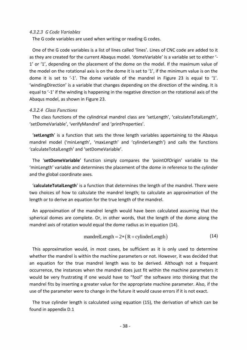
- 38 -
4.3.2.3 G Code Variables
The G code variables are used when writing or reading G codes.
One of the G code variables is a list of lines called ‘lines’. Lines of CNC code are added to it
as they are created for the current Abaqus model. ‘domeVariable’ is a variable set to either ‘-
1’ or ‘1’, depending on the placement of the dome on the model. If the maximum value of
the model on the rotational axis is on the dome it is set to ‘1’, if the minimum value is on the
dome it is set to ‘-1’. The dome variable of the mandrel in Figure 23 is equal to ‘1’.
‘windingDirection’ is a variable that changes depending on the direction of the winding. It is
equal to ‘-1’ if the winding is happening in the negative direction on the rotational axis of the
Abaqus model, as shown in Figure 23.
4.3.2.4 Class Functions
The class functions of the cylindrical mandrel class are ‘setLength’, ‘calculateTotalLength’,
‘setDomeVariable’, ‘verifyMandrel’ and ‘printProperties’.
‘setLength’ is a function that sets the three length variables appertaining to the Abaqus
mandrel model (‘minLength’, ‘maxLength’ and ‘cylinderLength’) and calls the functions
‘calculateTotalLength’ and ‘setDomeVariable’.
The ‘setDomeVariable’ function simply compares the ‘pointOfOrigin’ variable to the
‘minLength’ variable and determines the placement of the dome in reference to the cylinder
and the global coordinate axes.
‘calculateTotalLength’ is a function that determines the length of the mandrel. There were
two choices of how to calculate the mandrel length; to calculate an approximation of the
length or to derive an equation for the true length of the mandrel.
An approximation of the mandrel length would have been calculated assuming that the
spherical domes are complete. Or, in other words, that the length of the dome along the
mandrel axis of rotation would equal the dome radius as in equation (14).
mandrelLength 2 R cylinderLength
(14)
This approximation would, in most cases, be sufficient as it is only used to determine
whether the mandrel is within the machine parameters or not. However, it was decided that
an equation for the true mandrel length was to be derived. Although not a frequent
occurrence, the instances when the mandrel does just fit within the machine parameters it
would be very frustrating if one would have to “fool” the software into thinking that the
mandrel fits by inserting a greater value for the appropriate machine parameter. Also, if the
use of the parameter were to change in the future it would cause errors if it is not exact.
The true cylinder length is calculated using equation (15), the derivation of which can be
found in appendix D.1

- 39 -
2 2mandrelLength 2 R - r cylinderLength (15)
‘printProperties’ prints a summary of all the relevant mandrel properties in the Abaqus
Message Area, while simultaneously calling the ‘verifyMandrel’ function to determine
whether the mandrel is within the mandrel properties.
The ‘verifyMandrel’ function checks the mandrel properties against the machine
parameters to ascertain whether the mandrel is within the machine parameters. If the
mandrel exceeds any of the parameters a statement is printed, including what part of the
mandrel that does not meet the requirements of the filament winding machine. As shown
below the name of the filament winding machine whose parameters are not met is also
printed. This is a precaution to ensure that the mandrel is tested against the right
requirements, in case the machine parameters have not been set properly.
if (self.radius > settings.maxMandrelRadius):
print "The mandrel radius is too great for the ",
settings.Name, " machine"
4.3.3 Material
The ‘material’ class is created to contain several materials commonly used in filament
winding. Each material should include all the relevant material properties and a string
specifying the name of the material. Currently it only contains the ‘carbon_epoxy’ material
with approximate values for the material properties.
4.3.4 CustomNode
A ‘CustomNode’ object is initiated using a mandrel object, an element on the Abaqus
model and a numerical value ‘node’. It contains a list of nodal coordinates (‘XYZ’) and a list of
radii (‘radii’) calculated using different coordinate combinations.
4.3.4.1 Class Variables
The ‘XYZ’ list is first created containing only zeroes and then filled with the appropriate
coordinate values. An introduction to scripting with Abaqus and explanation of the nodes
and elements structure can be found in section 2.3.2 2.3.3 . Node coordinates are accessed
and set using the following command structure, which extracts the x-coordinate value for
the relevant node:
self.XYZ[X_AXIS] = mandrel.nodes[element.connectivity[node]]
.coordinates[X_AXIS]
To easier understand the command it can be shortened thusly:
nodeID = element.connectivity[node]
self.XYZ[X_AXIS] = mandrel.nodes[nodeID].coordinates[X_AXIS]
‘element’ is an element from the model elements list and ‘node’ is a numerical value for
the node’s position in the connectivity list.
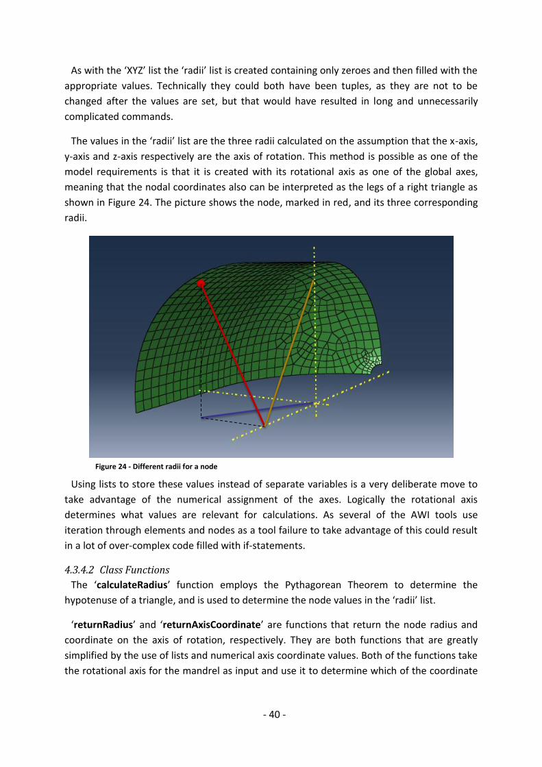
- 40 -
As with the ‘XYZ’ list the ‘radii’ list is created containing only zeroes and then filled with the
appropriate values. Technically they could both have been tuples, as they are not to be
changed after the values are set, but that would have resulted in long and unnecessarily
complicated commands.
The values in the ‘radii’ list are the three radii calculated on the assumption that the x-axis,
y-axis and z-axis respectively are the axis of rotation. This method is possible as one of the
model requirements is that it is created with its rotational axis as one of the global axes,
meaning that the nodal coordinates also can be interpreted as the legs of a right triangle as
shown in Figure 24. The picture shows the node, marked in red, and its three corresponding
radii.
Using lists to store these values instead of separate variables is a very deliberate move to
take advantage of the numerical assignment of the axes. Logically the rotational axis
determines what values are relevant for calculations. As several of the AWI tools use
iteration through elements and nodes as a tool failure to take advantage of this could result
in a lot of over-complex code filled with if-statements.
4.3.4.2 Class Functions
The ‘calculateRadius’ function employs the Pythagorean Theorem to determine the
hypotenuse of a triangle, and is used to determine the node values in the ‘radii’ list.
‘returnRadius’ and ‘returnAxisCoordinate’ are functions that return the node radius and
coordinate on the axis of rotation, respectively. They are both functions that are greatly
simplified by the use of lists and numerical axis coordinate values. Both of the functions take
the rotational axis for the mandrel as input and use it to determine which of the coordinate
Figure 24 - Different radii for a node

- 41 -
values or radii to return. If the values had not been set in lists these functions would have
had to consist of several if-statements testing for the rotational axis, as shown below:
def returnAxisCoordinate(self, rotationalAxis):
if mandrel.rotationalAxis == X_AXIS:
return self.X
if mandrel.rotationalAxis == Y_AXIS:
return self.Y
if mandrel.rotationalAxis == Z_AXIS:
return self.Z
Instead the function looks much simpler:
def returnAxisCoordinate(self, rotationalAxis):
return self.XYZ[rotationalAxis]
The last ‘customNode’ function is ‘printProperties’, which prints the values in the two class
variables. This function serves no purpose in the use of the tools, but is quite practical when
debugging or adding to the software.
4.3.5 CNCLine
‘CNCLine’ is a class for tool generated G code lines.
A ‘CNCLine’ object is initiated with all the relevant line variables, rounds them down to five
digits, and formats them into a string, ‘string’, which is then entered into the text file for the
CNC program. Each ‘CNCLine’ object is added to the mandrel variable ‘lines’ where it can be
easily extracted later. The object also has variables for each of the line variables ‘N’, ‘X’, ‘Y’,
‘Z’ and ‘W’. These separate line variables serve two purposes. They ensure easy access
without having to search through the string, and they store the accurate value, not the
rounded one.
Rounding the variables is not ideal, but practical all the same. Numerical errors will forever
be an issue, whether it is a computational error or a human error. To avoid the issue of
accumulated numerical errors as much as possible it is preferable to round any and all
numerical values at the last possible moment. For this reason the rounding of the machine
variables is done at this step, and only in the ‘string’ variable.
4.3.6 GCode
This class includes all the relevant G Code variables, like the sequence number, the
sequence incremental value and variables for the total movement in each axis direction.
Upon initiation the ‘GCode’ class opens or creates the appropriate text file and adds
several opening lines and comments to the top of the file. Lastly the first program line,
containing the proper preparatory commands, is inserted with the sequence number ‘10’.
The result is shown in Figure 25.

- 42 -
The class also contains a function that adds a program block to the text file while
simultaneously checking whether the movement along any of the axes exceeds the machine
limits. If the physical machine boundaries are overstepped the function will print statements
of in which direction the error occurred. In the common case, when the boundaries are not
exceeded, the function adds the program block to the list of program blocks and the writes
the block into the text file.
4.3.7 LayupConstruction
‘LayupConstruction’ is a class used while adding layup to an Abaqus model.
4.3.7.1 General variables
Currently the only general variable is the ‘material’ variables, which stores the material
used for the winding layup.
4.3.7.2 Movement Variables
These variables track the movement of the mandrel during the winding process.
‘P1’ stores the coordinate value of the current position on the mandrel. Before winding has
begun it is assumed to begin at the dome tip on the rotational axis and ‘0’ on the two
remaining axes. The variable ‘P2’ is the next position on the mandrel determined by the
rotation of the mandrel and the movement along the rotational axis.
Considering the plane created by the horizontal and vertical mandrel axes ‘P1’ and ‘P2’
becomes points on a circle. The ‘crossesHorizontal’ and ‘crossesVertical’ variables (initially
set as ‘False’) describe whether the two points are located in the same quadrant or if ‘P2’ is
on the other side of one of one of the axes. Figure 26 shows the two different possibilities
for placement of ‘P2’. For the red instance of ‘P2’, located in quadrant II, the vertical axis, ‘V’
has been crossed and ‘crossesVertical’ set to ‘True’.
Figure 25 - GCode opening lines

- 43 -
4.3.8 Assembly
The ‘assembly’ class is used to perform a visual crash test for a CNC program. It includes a
function that creates a part called ‘feedEye’, which is to be placed in an assembly together
with the mandrel part. In the assembly the ‘move’ function is used to move the feed-eye in
relation to the mandrel according to the CNC codes. The ‘move’ function translates the feed-
eye incrementally using the Abaqus ‘translate’ command, then immediately redraws the
feed-eye in the new position, as shown below:
self.assemblyDir.translate((self.feedEye, ), newCoords)
session.viewports['Viewport: 1']
.view.setValues(drawImmediately = True)
P2
P2 V
H
IV III
I II
P1
Figure 26 - Placement of P2

- 44 -
4.4 MandrelProperties.py This module contains functions that determine the mandrel properties for the relevant
Abaqus model and adds them to the ‘CylindricalMandrel’ object ‘mandrel’.
Determining the geometrical properties of a part is, in most cases, quite easy by visual
inspection. It is, however, not as simple to accomplish by scripting, especially when the goal
is to create a versatile script. Consequently some of the functions might appear inefficient,
but the procedures have been specifically chosen to promote flexibility.
4.4.1 determineRotationalAxis
The ‘determineRotationalAxis’ function discerns the rotational axis of an axisymmetric
mandrel by comparing the different nodal radii.
4.4.1.1 Approach
The mandrel is axisymmetric, and it was resolved that the best way to determine its axis of
rotation would be to somehow compare radii in different directions for a locus on the
mandrel. As the element nodes are already pre-defined loci with global coordinate values,
the logical step was to use these in this function. To calculate the radii in different directions
the best approach would be using the Pythagorean Theorem for each global coordinate
plane, which resulted in the ‘CustomNode’ class, its ‘radii’ variable and its ‘calculateRadius’
function.
The choice was made to design a function that iterates through the ‘elements’ list of a
‘CylindricalMandrel’ object comparing nodal variables until the rotational axis of the model
has been found.
4.4.1.2 Design Choices
To iterate through the ‘elements’ list of a ‘CylindricalMandrel’ object there were two
choices considered; a while loop or a for loop. Normally, when iterating through a list, a for
loop is the obvious choice. However, in this instance, it is not necessary to iterate through
the complete list and a while loop was considered as well. There are no great differences
between the two choices, except that in a for loop it would be necessary to utilise the break
statement and in a while loop utilise a counter to iterate through the list. Ultimately the
choice fell on the while loop, simply because it makes the code more intuitive to read.
while mandrel.rotationalAxis == 'undetermined':
For the choice of what nodes to compare, it was decided that, to avoid a for loop within
the while loop, the first node in the ‘connectivity’ list of two elements should be compared.
Alternatively one could iterate through the nodes on an element instead, but as there is no
real difference between the two in terms of result the idea of a for loop was rejected to keep
the code as structured as possible. A consequence of this choice, combined with the desire
to make flexible software capable of handling any type of mesh, is that the two nodes
compared might actually be the same node. If the mesh is unstructured, or a triangular

- 45 -
mesh, the elements do not necessarily have the same amount of nodes and are not oriented
identically. In some cases the first node in the ‘connectivity’ list of two elements will be the
same node; therefore a test comparing the coordinates of the two nodes was implemented.
As a precaution, both during development and later, it was decided to insert an option for
manual input of the rotational axis. If ever the function should fail to determine the
rotational axis of the relevant mandrel model it does not necessarily cause the software to
crash.
During the testing of the function on different types of meshes it was discovered that in
some, very rare, cases it was impossible to determine the rotational axis of the model
because of very small differences in the calculated radii (for example: 125,00001468 !=
124,999998575). An educated guess is that this is caused by slight inaccuracies in the nodal
placement, a phenomenon the author has also observed in other 3D modelling software.
With such high accuracy in the calculation of the radii the small inaccuracies in nodal
placement cause false negatives. To compensate for this it was decided to round the values
down to five decimals as they are compared.
Normally rounding variables is frowned upon as it causes numerical errors that stack.
However, in this instance it has no effect on any actual values and does therefore not pose a
problem. As the variables are only rounded when they are compared, but keep their original
exact value in the node object, and the rounded value is not used for any form of calculation
this approach has no negative effect on the rest of the tools.
In comparing the radii there is a slight chance of the test returning a false positive. This
happens if the nodal coordinates are both too close to the point of origin for the model, the
global (0, 0, 0). In such a case the ‘radii’ value for the nodes could be zero (and thereby
equal) in a different direction than the one indicating the correct rotational axis. To avoid
this issue it was determined that a fail-safe variable should be used to check that the
rotational axis determined is indeed the right one. Before finally setting the axis of rotation
this fail-safe variable should be set to equal an axis for which the nodal ‘radii’ value has been
determined equal and then compared to the relevant axis when the nodal values are again
equal. This means that the function must register the same axis as the rotational axis twice
before it sets the ‘rotationalAxis’ variable of a ‘cylindricalMandrel’ object and exits the loop.
In other words two sets of elements must to have the same ‘radii’ value for the rotational
axis to be set and the function completed.
4.4.1.3 Mode of Operation
A while loop is utilised to iterate through all the elements in the model ‘elements’ list until
the rotational axis has been found. Moving through the list, nodal ‘radii’ values for the first
node (‘currentNode’) in the connectivity list of each element is compared to those of the
next element in the list (‘nextNode’).

- 46 -
At the top of the function a variable ‘counter’ is set equal to zero, and for each run through
the loop incremented by one. ‘counter’ is used to move through the ‘elements’ list so that in
turn a ‘customNode’ object can be initiated.
element = mandrel.elements[counter]
currentNode = classes.CustomNode(mandrel, element, 0)
If ‘counter’ has reached the end of the ‘elements’ list without being able to determine the
rotational axis, the function prompts for manual input through the Abaqus GUI.
if counter >= len(mandrel.elements):
print "it was not possible to determine the rotational
axis"
#ask for manual input through GUI
rotationalAxis = getInput(
'Enter the numerical value for the rotational Axis:
\n(X-Axis = 0, Y-Axis = 1, Z-Axis = 2)')
mandrel.rotationalAxis = int(rotationalAxis)
Whenever the ‘counter’ has still not reached the end of the ‘elements’ list the ‘nextNode’
object is created and the two nodes ‘currentNode’ and ‘nextNode’ compared.
To ensure that the two nodes compared are not in reality the same node, the function
compares their coordinate values. If they are equal, they are the same node and the loop is
continued.
For each of the axes (X, Y, Z) the nodal ‘radii’ values are rounded down to five decimals and
compared; are the nodal values identical in any direction a variable, ‘test’, is checked. If ‘test’
is not equal to the axis in question it is either the first instance of nodal equality, or a
previous comparison has returned a different axis. Regardless, the ‘test’ variable is set to the
current axis and the loop continued. If ‘test’ is equal to the rotational axis in question, the
rotational axis of the mandrel is set, and the loop is exited.
if round(currentNode.Radii[X_AXIS],5) ==
round(nextNode.Radii[X_AXIS], 5):
# if the fail-safe variable is 'None' or another axis
if test != X_AXIS:
test = X_AXIS
# if the previous comparison also returned this axis, the
rotational axis is set
elif test == X_AXIS:
mandrel.rotationalAxis = X_AXIS
mandrel.H = Z_AXIS
mandrel.V = Y_AXIS
As can be seen from the code segment above, the ‘determineRotationalAxis’ function
simultaneously sets the horizontal and vertical axis for the mandrel when the rotational axis
of the mandrel has been found.

- 47 -
4.4.2 determineRadii
The ‘determineRadii’ function determines the radius of the cylinder and the dome opening
radius of an Abaqus mandrel model.
4.4.2.1 Approach
The cylindrical radius and the radius of the dome opening are the greatest and smallest
radii respectively on the Abaqus mandrel model.
It was determined that the best way to discover the two radii would be to iterate through
all the elements of a model and compare the different radii. Normally it is not considered
ideal to iterate through a list such as this, especially as it is likely to be quite large as the
elements on a model is shrunk for accuracy of analysis. Nevertheless, it was deemed the
best solution.
4.4.2.2 Design Choices
One of the solutions considered to avoid an iteration loop was to somehow sort the
elements into two separate lists; one containing all the cylindrical elements, and one
containing the elements of the dome. This would have required iteration through all of the
elements to first determine the cylindrical radius, and then another iteration to sort the
elements. As such sorting of the elements would only be useful for this specific task, and it
would require more iterations than simply comparing all the radii it was rejected. It was
concluded that, as the only known variable is the rotational axis of the model, an iteration
loop would be the best choice.
As the orientation of the elements is unknown it was deemed necessary to iterate through
all of the nodes of an element and not just pick one at random as is done in
‘determineRotationalAxis’. For the cylindrical part of the model it would most likely not have
posed a problem, but for the dome opening it is imperative that each node is inspected to
ensure that the correct value for the minimum radius is found. Figure 27 illustrates a case
where a random node would not return the correct radial value.
Figure 27 - Node returning wrong radius

- 48 -
To iterate through all of the element nodes a variable ‘nodesOnElemen’ is utilised. This was
done to compensate for the fact that the function is intended to work for any type of mesh;
unstructured as well as structured.
There is no knowledge of the size of the model, and therefore it is impossible to set
arbitrary values for comparison. The ‘maxRadius’ could have been set to equal zero, but for
the ‘minRadius’ variable there is no value that will always be bigger than the minimum
radius of an actual Abaqus model. One solution would be to assume a value of, for example,
100 000, but it is still not completely certain that the minimum radius will always be smaller
than this value. It could happen that the units are set in micro metres, or that the mandrel to
be wound is humongous.
The simple, and obvious, solution that was decided upon is that of initiating ‘maxRadius’
and ‘minRadius’ as ‘None’ and then set them to equal the radius of the first node of the first
elements to serve as points of comparison. This way the initial values for ‘maxRadius’ and
‘minRadius’ will always be lesser than, greater than or equal to the following nodal radii.
During the development process of the AWI Tools the ‘pointOfOrigin’ value of the
‘CylindricalMandrel’ class was created. As this value, by definition, is located at the tip of the
mandrel (or in other words at the same locus as the minimum radius) it was decided that the
logical way to set this variable would be along with the minimum radius. In most cases an
effort has been made to keep functions separate and simple, not performing too many tasks
at once. However, it was determined that such a simple task as setting this variable did not
warrant an additional function with an iteration loop.
4.4.2.3 Mode of Operation
A double for loop is utilised to iterate through all the nodes on all the elements in the
‘elements’ list of an Abaqus model comparing the radii. For each node the local radius is
compared to the function variables ‘minRadius’ and ‘maxRadius’.
For each element the number of nodes is determined (‘nodesOnElement’), and the nodal
properties for each node investigated.
for element in mandrel.elements:
nodesOnElement = len(element.connectivity)
# iterate through the nodes
for i in range(nodesOnElement):
currentNode = classes.CustomNode(mandrel, element, i)
tempRadius =
currentNode.returnRadius(mandrel.rotationalAxis)
For the first node on the first element the ‘minRadius’ and ‘maxRadius’ variables are set to
equal the nodal ‘tempRadius’. This then serves as the point of comparison for the rest of the
nodes. The ‘tempRadius’ value of each following node is compared to the function variables

- 49 -
‘minRadius’ and ‘maxRadius’. If the local radius is less than ‘minRadius’ or greater than
‘maxRadius’ the appropriate value is replaced by the local ‘tempRadius’.
# set point of comparison on the first iteration
if minRadius == None:
minRadius = tempRadius
maxRadius = tempRadius
# in case the first node is on the dome opening
mandrel.pointOfOrigin =
currentNode.returnAxisCoordinate(mandrel.rotationalAxis)
elif tempRadius < minRadius:
minRadius = tempRadius
mandrel.pointOfOrigin =
currentNode.returnAxisCoordinate(mandrel.rotationalAxis)
elif tempRadius > maxRadius:
maxRadius = tempRadius
Simultaneously as the nodal radii are compared, the ‘pointOfOrigin’ value of the ‘mandrel’
object is set whenever the ‘minRadius’ value is replaced.
4.4.3 determineLength
The ‘determineLength’ function calculates the length of the cylindrical part of an Abaqus
mandrel model.
4.4.3.1 Approach
To determine the length of the cylindrical part of a mandrel it is necessary to determine the
extreme points of the cylinder along the axis of rotation.
The choice was made to accomplish this in the same way as with the model radii. By means
of iterating through all of the elements comparing nodal attributes. The difference being
that in this case it is the nodal coordinate on the axis of rotation that is compared, and not
radii.
4.4.3.2 Design Choices
As with the ‘determineRadii’ function a double for loop was deemed necessary, including
the ‘nodesOnElement’ set to the number of nodes for each element. See section 4.4.2.2 for
a closer explanation of the reasons behind this decision.
To distinguish between the elements on the cylindrical part of the mandrel and the
elements on the dome the nodal radius was compared to the radius of the
‘CylindricalMandrel’ object ‘mandrel’. It was considered whether this task would be simpler,
and require fewer actions, if the elements were sorted as explained in section 4.4.2.2 .
However, it was determined that it would most likely not result in more efficient code and
was therefore not worthwhile.

- 50 -
4.4.3.3 Mode of Operation
A double for loop iterated through the elements in a ‘CylindricalMandrel’ object ‘elements’
list. When appropriate the nodal coordinate on the rotational axis for all the element nodes
are compared to the function variables ‘minLength’ and ‘maxLength’ to determine the
extreme points of a cylinder.
For each element the number of nodes is determined (‘nodesOnElement’), and the nodal
properties for each node investigated. If the local node radius is not equal to the radius of
the ‘mandrel’ object, the current element is not located on the cylinder and the for loop is
continued.
if round(tempRadius, 5) != round(mandrel.radius, 5):
break
For the first node on the first element on the cylindrical part of the mandrel the
‘minLength’ and ‘maxLength’ variables are set to equal the nodal position on the rotational
axis of the ‘mandrel’ object. This then serves as the point of comparison for the rest of the
nodes. A variable, ‘rotAxCoordinate’, is compared to the function variables ‘minLength’ and
‘maxLength’ for each of the following nodes on the cylinder. If the local ‘rotAxCoordinate’ is
less than ‘minLength’ or greater than ‘maxLength’, the appropriate value is replaced.
if minLength == None:
minLength = rotAxCoordinate
maxLength = rotAxCoordinate
elif rotAxCoordinate < minLength:
minLength = rotAxCoordinate
elif rotAxCoordinate > maxLength:
maxLength = rotAxCoordinate
Once the for loop has finished iterating through the elements the ‘CylindricalMandrel’ class
function ‘setLength’ is called and the ‘minLength’ and ‘maxLength’ variables are used to
calculate the length of the cylindrical part of the model.
mandrel.setLength(minLength, maxLength)
4.4.4 setProperties
‘setProperties’ is the execution function of the ‘mandrelProperties’ module. The function
executes the ‘determineRotationalAxis’ function, ‘determineRadii’ function and the
‘determineLength’ function, one after the other, to determine and calculate the mandrel
properties.
Lastly, the ‘printProperties’ function of the ‘CylindricalMandrel’ object ‘mandrel’ is
executed and the properties of the Abaqus mandrel model printed.
print 'Mandrel Properties: '
print '-----------------------------------------'
mandrel.printProperties(settings)

- 51 -
4.4.4.1 Flowchart of Execution Function
settings
mandrel determineRotationalAxis
determineRadii
determineLength
Mandrel.printProperties

- 52 -
4.5 GCode.py The ‘GCode.py’ module is intended to include all the functions necessary to generate a CNC
program based on the mandrel properties of an Abaqus model.
Initially it was the intention that this module should include functions for the kinematic
equations for a filament winding machine, but due to the unforeseen circumstances
described in chapter 3.3 the module is currently incomplete.
4.5.1 createCNCprogram
The ‘createCNCprogram’ function generates a CNC program for the relevant Abaqus
mandrel model.
4.5.1.1 Approach
This function will most likely be the execution file of the ‘GCode’ module. It is created as a
means of collecting the variables for blocks of CNC code and writing it to a file and the
‘mandrel’ object ‘lines’ variable.
4.5.1.2 Design Choices
It was determined that the filename of the CNC program should be unique and descriptive
to make it easily identifiable. Consequently it was decided that the filename should include
the Abaqus model name and the model part name.
Also, for clarity, it was decided to include a print statement after the completion of the CNC
program to inform that the program has been generated, and for which Abaqus mandrel
model.
4.5.1.3 Mode of Operation
First, the filename of the CNC program is set.
fileName= "{0}_{1}".format(mandrel.modelName, mandrel.partName)
Secondly, a ‘GCode’ class object is initiated with the filename, creating the CNC program
file and writing the topmost comment lines. Then the lines (currently a set of lines with
random values for the variables) are added to both the CNC program file and the ‘lines’
variable of the ‘CylindricalMandrel’ object ‘mandrel’.
Once the CNC program has been generated a statement is printed in the Abaqus Message
Area, including the ‘printProperties’ function of the ‘mandrel’ object.
print "a CNC-program has been created for: "
mandrel.printProperties(settings)
As the function is run through Abaqus, the text file will be located in the Abaqus work
directory.

- 53 -
4.6 layup.py The ‘layup.py’ module contains the functions necessary to add the approximation of a
filament winding layup to an Abaqus mandrel model based on blocks of CNC code.
Adding layup to an Abaqus mandrel model is a challenge, and its solution involves
approximations and assumptions. Two different solutions were considered to solve the
problem, and the decision of which to choose was done based on its determined accuracy.
Solution 1:
As long as the geodesic winding technique used the winding angle for a point on the
mandrel can easily be calculated by means of Clairaut’s equation (1). If one assumes a known
number of complete layers of winding on the mandrel a layup of [α/-α] can be added to the
elements for each layer. It should be noted that this assumption disregards the crossover
points of a winding layup. Also, depending on the shape and size of the elements further
assumptions and approximations would have had to be made in regards to, for example, the
winding angle across the dome. On the cylindrical part of the mandrel the winding angle
would remain constant, but crossing the dome it changes rapidly to the required angle of 90°
at the dome opening. Accounting for this fact could, amongst others, be done by calculating
the mean winding value for each element or by choosing the middle point of the element to
calculate the winding angle.
In addition to the approximation being a poor one, this solution lacks flexibility. There is no
accounting for the different layers that form in the winding process, and having been
modelled as a uniform layer it does not actually correspond to any actual physical part. It
does, however, suit a preliminary model where no CNC program has been created yet. It is,
most likely, possible to analyse a model with such a layup and use the results as a rough
draft of the capabilities of the finished part. This should, however, be investigated more fully
before a hypothetical implementation.
Solution 2:
In geodesic winding the fibres are placed on the shortest possible path between two points
on the mandrel, a fact that can be taken advantage of when creating an approximate
winding layup on an Abaqus model. If the path between the two points ‘P1’ and ‘P2’ is
projected into a two-dimensional plane it can be approximated to a straight linear line under
certain conditions. This approach has been detailed in appendix D.3
Under the conditions that P1x or P2x cannot be too close to the radial value, and that they
must be located in the same or adjoining quadrants, the path can be considered linear
between two points. The linear equation for this straight line can easily be derived from the
coordinates of those two points. With this line in place the elements can be projected into
the same plane and it can be determined whether each element lies on the winding path or
not.

- 54 -
Using this approach with ‘P1’ and ‘P2’ as the starting and ending points of a CNC program
block each element will end up with a unique combination of plies as a layup. Although an
approximation, this results in a layup whose plies will correspond directly to a part wound
with the relevant CNC program. As far as this author knows there are no other software
solutions that include this functionality of using FEA software to create a model that directly
corresponds to a real part. It was decided, therefore, to start developing this solution, as it is
more advanced.
4.6.1 addMaterial
The ‘addMaterial’ function adds a carbon/epoxy material to the ‘LayupConstruction’ object
‘layup’ and adds the material to the relevant Abaqus mandrel model.
4.6.1.1 Approach
The choice to create this function was made for structure. The material needed to be
added to the Abaqus mandrel model, and the name of the material accessed for each layup
to be added.
4.6.1.2 Design Choices
It was decided to keep the Abaqus commands that add a material to an Abaqus model
separate as they are long and appear unstructured at first glance. Having them collected in a
function has the added bonus of adding readability to the code as well.
To avoid having to send the ‘Name’ variable of the ‘material’ object back and forth
between functions it was decided to connect the material to the ‘layup’.
4.6.1.3 Mode of Operation
The ‘carbon_epoxy’ material is set as the layup material.
layup.material.carbon_epoxy()
A material with the same name as the layup material is added to the Abaqus part.
mdb.models[mandrel.modelName]
.Material(name = layup.material.Name)
Then the material properties are set using the Abaqus material commands (the complete
commands can be viewed in E.4
mdb.models[mandrel.modelName]
.materials[layup.material.Name].Elastic(…)
mdb.models[mandrel.modelName]
.materials[layup.material.Name].Density(…)

- 55 -
4.6.2 readGCodes
The ‘readGCodes’ function reads a CNC program block and extracts from it the rotation of
the mandrel and the lateral movement of the carriage along the rotational axis of the
mandrel.
4.6.2.1 Approach
A CNC program block read from a file is read as a string. It was decided that the most
practical approach to search through a string for matches of the relevant parameters would
be to use the built-in Python regular expressions. An introduction to these can be found
in[31] or [32].
4.6.2.2 Design Choices
During the development, it was determined to start by assuming the same axis notations
for the filament winding machine as the “MAW 20 LS 4/1” from Mikrosam. The relevant axes
for this function would then be the rotation of the mandrel, ‘X’, and the lateral movement of
the carriage, ‘Y’.
To account for the comment lines and the first line of modal commands in the CNC
program the Python exception handling interface is used. If the ‘X’ and ‘Y’ values are not
found in the string, the ‘AttributeError’ is raised. In this case the lack of the ‘X’ and ‘Y’ values
in the string only means that the line is one of the top lines of comments or modal
commands.
It was observed that a CNC program can be written with either points or commas. As
Abaqus only accepts floats using points it was determined to utilise the Python ‘replace’
function to ensure that the float values will be in the correct format.
4.6.2.3 Mode of Operation
A variable, ‘line’, from a CNC program is sent to the function, and matches for the ‘X’ and
‘Y’ values searched for.
matches = re.search(
r'\A N(\d+) \s+ X(\d+(,\d+)?) \s+ Y(\d+(,\d+)?)',
line, flags=re.M | re.S | re.X)
If matches are found, a tuple ‘(X, Y)’ is retuned, but if an exception is raised the function
simply returns nothing.
4.6.3 Sign
‘Sign’ is a simple function that determines the sign of a numerical variable. It was
implemented to increase readability of the code as it negates the need for several identical if
statements.
If the value is negative it returns ‘-1’ and if it is positive it returns ‘1’.
- 56 -
4.6.4 calculateP2
‘calculateP2’ is a function that, based on the rotation of the mandrel, calculates the end
point of a CNC program block, ‘P2’.
4.6.4.1 Approach
As the lateral movement along the axis of rotation can be extracted directly from the CNC
program block, the position of ‘P2’ on the axis of rotation can easily be calculated.
Determining the two remaining coordinate values of ‘P2’, however, is not as simple.
The rotation of the mandrel, ‘X’, translates as an angle in the plane formed by the
horizontal and vertical axes of the mandrel. Therefore it was decided that the best way to
determine the coordinates of ‘P2’ would be to use basic trigonometry. The mathematics
behind the approach have been detailed in appendix D.2
4.6.4.2 Design Choices
The choice of using trigonometry was made because the lateral movement along the axis
of rotation is so easily calculable. With this coordinate determined the two others can be
considered independently of the third one, and the problem is somewhat simplified. With
only two axes to consider the problem is transformed into a unit circle of radius ‘R’ passing
through the two points ‘P1’ and ‘P2’, as shown in Figure 28. As the coordinates of ‘P1’ and
the angle, ‘X’, between the two points is known the coordinates of ‘P2’ can be calculated.
To simplify the problem further an assumption was made that the rotation of the mandrel
will be small enough that ‘P1’ and ‘P2’ will always be located in either the same quadrant or
adjoining quadrants of the unit circle. This decision limits the problem to eight different
permutations of placement. This approach, and pictures of all placements of ‘P2’, has been
further detailed in D.2
P2
V
H
IV III
I II P1
Figure 28 – Simplified problem
X

- 57 -
Due to the fact that the coordinate values will vary in sign the mode of calculating the
coordinates of ‘P2’ will vary depending on the quadrantic placement of the two points. An
effort was made to find an approach that was as uniform as possible. The result was a
method based on the rotation of the mandrel, ‘X’, the angle between ‘P1’ and the horizontal
axis, ‘U’, and the angle between ‘P2’ and the horizontal axis, ‘W’. Using this method the
approach to calculating ‘W’ is the same for quadrants I and III and quadrants II and IV.
The angle ‘U’ is calculated using equation (16), where ‘P1V‘ is the coordinate value of ‘P1’
on the vertical axis, and ‘P1H‘ the coordinate value on the horizontal axis.
V
H
1P1
U tanP1
(16)
For quadrants I and III the calculation of ‘W’ is as follows:
If the added value of the angles ‘U’ and ‘X’ is less than 90° the two points are located in the
same quadrant (I and III respectively), and the angle ‘W’ is calculated using equation (17).
W U X (17)
Are ‘P1’ and ‘P2’ located in adjoining quadrants (II and IV respectively) the angle, ‘W’, is
calculated using equation (18).
W U X (18)
For quadrants II and IV the calculation of ‘W’ is as follows:
If the added value of the angles ‘U’ and ‘X’ are less than 90° the two points are located in
the same quadrant (II and IV respectively) the angle, ‘W’, is calculated using equation (19).
W U X (19)
Are ‘P1’ and ‘P2’ located in adjoining quadrants (III and I respectively) the angle, ‘W’, is
calculated using equation (20).
W X U (20)
To account for the change of sign between ‘P1’ and ‘P2’ the ‘sign’ variable for the
appropriate axis is changed whenever the two points are not located in the same quadrant.
In addition one of the variables of the ‘layupConstruction’ object ‘layup’ is changed. If ‘P1’ is
located in quadrant I and ‘P2’ in quadrant II ‘crossesVertical’ is set to ‘True’ and if ‘P1’ is
located in quadrant II and ‘P2’ in quadrant III ‘crossesHorizontal’ is set to ‘True’ and so
forth.
Once the angle ‘W’ has been determined the leg lengths of a triangle formed by ‘P2’ and
the horizontal axis is calculated using equations (21) and (22).

- 58 -
legH signH R cos W
(21)
legV signV R sin W
(22)
Without the ‘sign’ variable these calculations would have resulted in the absolute leg
lengths of ‘P2’, meaning its coordinates had it been located in quadrant I. With the use of
the ‘sign’ variables this problem is avoided.
It should be noted that these calculations assume ‘X’ to be set in radians. This might not be
the case and should be checked to ensure that the function works, but a hypothetical
conversion from radians to degrees will not pose a problem.
To calculate the lateral movement along the axis of rotation it was decided to implement a
‘cylindricalMandrel’ class variable ‘windingDirection’. The coordinate system assumed when
deriving the equations was set with the rotational axis in the opposite direction of that of
the filament winding machine coordinate system. This means that it is necessary to reverse
the sign of the ‘Y’ movement variable before it is employed.
4.6.4.3 Mode of Operation
‘P1’, the rotation of the mandrel, ‘X’, and the lateral feed-eye movement, ‘Y’ are used to
calculate the coordinate values of the end point of a CNC program block, ‘P2’.
A variable for the point ‘P1’ is created and the signs for its horizontal and vertical
coordinate values, ‘signH’ and ‘signV’, are determined. Then the angle, ‘U’ between ‘P1’ and
the horizontal axis is calculated.
P1 = layup.P1
# determine what quadrant P1 is located in
signH = sign(P1[mandrel.H])
signV = sign(P1[mandrel.V])
# calculate the angle between P1 and the horizontal axis
U = math.atan2(abs(P1[mandrel.V]),abs(P1[mandrel.H]))
These values are then used to determine the quadrantic placements of ‘P1’ and ‘P2’. If the
two ‘sign’ values are equal (both either positive or negative) ‘P1’ is located in quadrant I or
quadrant III.
# if the coordinates of P1 are in quadrant I or III
if (signH == signV):
# if P1 and P2 are in the same quadrant
if (U+X) < (math.pi/2):
W = U+X
else:
W = math.pi - (U+X)
signH *= -1
layup.crossesVertical = True

- 59 -
If the ‘sign’ values are not equal, ‘P1’ is located in quadrant II or IV.
# if the coordinates of P1 are in quadrant II or IV
else:
# if P1 and P2 are in the same quadrant
if (X < U):
W = U-X
else:
W = X-U
signV *= -1
layup.crossesHorizontal = True
For each case the angle between ‘P2’ and the horizontal axis, ‘W’, is calculated. When the
two points ‘P1’ and ‘P2’ are not located in the same quadrant two additional variables are
changed. Depending on which axis has been crossed the ‘signH’ and ‘crossesHorizontal’ or
the ‘signV’ and ‘crossesVertical’ are altered. The ‘sign’ value is multiplied by ‘-1’ to change its
sign, and the second variable is set to ‘True’.
Lastly, the coordinates of ‘P2’ are calculated using the cosine and sine of the angle ‘W’.
legH = signH * (mandrel.radius * math.cos(W)) #horizontal
leg
legV = signV * (mandrel.radius * math.sin(W)) #vertical leg
legLateral = P1[mandrel.rotationalAxis] +
mandrel.windingDirection * Y
The ‘P2’ list of the ‘layupConstruction’ object ‘layup’ is filled.
### set values for P2
layup.P2[mandrel.rotationalAxis] = legLateral
layup.P2[mandrel.V] = legV
layup.P2[mandrel.H] = legH
4.6.5 collectBoxElements
The ‘collectBoxElements’ function collects a set of elements between the points ‘P1’ and
‘P2’ in a list using the Abaqus ‘getByBoundingBox(…)’ command.
4.6.5.1 Approach
With the point of origin and the end point of a CNC program block in place, it is possible to
iterate through all of the elements on a model to determine which ones cross the winding
path. However, to avoid iteration through the complete model it was decided to take
advantage of the Abaqus ‘getByBoundingBox(…)’ command. As the coordinates of the two
points, ‘P1’ and ‘P2’, are known this function is ideally suited for this purpose.
4.6.5.2 Design Choices
The ‘getByBoundingBox(…)’ requires the maximum and minimum coordinate values of the
bounding box as arguments. Consequently the coordinate values of ‘P1’ and ‘P2’ need to be

- 60 -
sorted for each axis. As the two points are not necessarily located in the same quadrant, it is
impossible to know which one of the points has the smaller or greater coordinate value in a
specific direction. To circumvent this problem it was decided to sort the coordinate positions
of ‘P1’ and ‘P2’ into two lists, ‘minCoords’ and ‘maxCoords’, independently of which point
the value originates from. These lists will then be used as arguments for the
‘getByBoundingbox(…)’ command.
In the cases where the points are not located in the same quadrant it is not sufficient to
use only the coordinate values of the points as arguments for ‘getByBoundingBox(…)’. It is
clear from Figure 29 that if the points are in separate quadrants, using only the maximum
and minimum coordinate values will result in a bounding box that does not encompass all
the relevant elements. The red box illustrates the correct bounding box, whereas the brown
stippled line illustrated where the topmost boundary of the box would have been with only
the coordinate values as boundary conditions. Therefore the ‘crossesHorizontal’ and
‘crossesVertical’ variables of the ‘layupConstruction’ class were created. If any of these
variables are ‘True’, an axis has been crossed and the minimum/maximum value in the
appropriate direction must be set to equal the mandrel radius, or the negative mandrel
radius, depending on the quadrants in question.
4.6.5.3 Mode of Operation
The Abaqus ‘getByBoundingBox(…)’ command is utilised to collect the elements between
two points, ‘P1’ and ‘P2’. Based on the coordinate values of ‘P1’ and ‘P2’ and their quadrant
on the unit circle, the maximum and minimum coordinates of the bounding box are
determined.
Two lists, ‘minCoords’ and ‘maxCoords’, are created and initially filled with zeroes, before
the ‘P1’ and ‘P2’ variables of the ‘layupConstruction’ object ‘layup’ are copied to the function
variables ‘P1’ and ‘P2’.
Figure 29 - Bounding box between P1 and P2
P
2
P1

- 61 -
The coordinate values for each list index in the ‘P1’ and ‘P2’ lists are compared and sorted.
The greater of the two values is placed in the ‘maxCoords’ list, and the smaller of the two in
the ‘minCoords’ list.
for i in range(3):
if (P1[i] < P2[i]):
minCoords[i] = P1[i]
maxCoords[i] = P2[i]
else:
minCoords[i] = P2[i]
maxCoords[i] = P1[i]
A test is run to check whether the ‘crossesHorizontal’ or ‘crossesVertical’ variables of the
‘layup’ object are set to ‘True’. If either one is ‘True’, depending on the quadrant placement
of ‘P1’, the ‘minCoords’ or ‘maxCoords’ list is changed in the appropriate direction to
encompass all the relevant elements.
# if an axis has been crossed the max/min variable
# must be mandrel radius to collect all elements
if layup.crossesHorizontal:
if sign(P1[mandrel.V]) > 0:
minCoords[mandrel.H] = -1* mandrel.radius
else:
maxCoords[mandrel.H] = mandrel.radius
if layup.crossesVertical:
if sign(P1[mandrel.H]) > 0:
maxCoords[mandrel.V] = mandrel.radius
else:
minCoords[mandrel.V] = -1*mandrel.radius
The Abaqus ‘getByBoundingBox(…)’ command is used, with the values of ‘minCoords’ and
‘maxCoords’ as arguments, to collect all the elements between ‘P1’ and ‘P2’ in a list.
4.6.6 collectLayupElements
The ‘collectLayupElements’ function iterates through the elements collected in the
‘collectBoxElements’ function and determines whether each element is located in the
winding fibre path or not.
4.6.6.1 Approach
To determine which elements are located in the winding path, the pathway is projected
into the plane formed by the rotational axis and either the horizontal or vertical mandrel
axis. For each element, its nodal coordinates are projected into the same plane and a check
is performed to ascertain whether the winding path crosses the element or not.
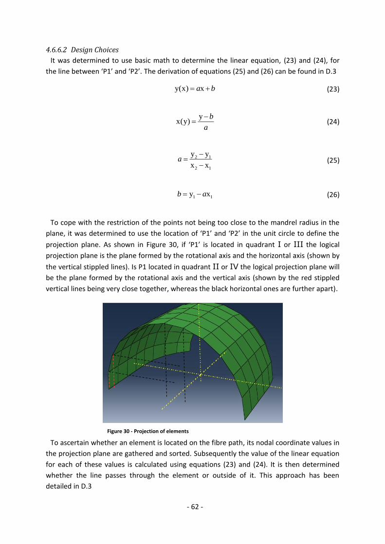
- 62 -
4.6.6.2 Design Choices
It was determined to use basic math to determine the linear equation, (23) and (24), for
the line between ‘P1’ and ‘P2’. The derivation of equations (25) and (26) can be found in D.3
y(x) xa b (23)
yx(y)
b
a
(24)
2 1
2 1
y y
x xa
(25)
1 1y xb a (26)
To cope with the restriction of the points not being too close to the mandrel radius in the
plane, it was determined to use the location of ‘P1’ and ‘P2’ in the unit circle to define the
projection plane. As shown in Figure 30, if ‘P1’ is located in quadrant I or III the logical
projection plane is the plane formed by the rotational axis and the horizontal axis (shown by
the vertical stippled lines). Is P1 located in quadrant II or IV the logical projection plane will
be the plane formed by the rotational axis and the vertical axis (shown by the red stippled
vertical lines being very close together, whereas the black horizontal ones are further apart).
To ascertain whether an element is located on the fibre path, its nodal coordinate values in
the projection plane are gathered and sorted. Subsequently the value of the linear equation
for each of these values is calculated using equations (23) and (24). It is then determined
whether the line passes through the element or outside of it. This approach has been
detailed in D.3
Figure 30 - Projection of elements

- 63 -
4.6.6.3 Mode of Operation
The variables ‘P1’ and ‘P2’ of the ‘layupConstruction’ object ‘layup’ are copied to the
function variables, ‘P1’ and ‘P2’.
Based on the quadrant placements of ‘P1’ and ‘P2’ and their coordinate values, the
constants ‘a’ and ‘b’ of a linear equation between the two points are determined.
if sign(P1[mandrel.H]) == sign(P1[mandrel.V]):
a = ((P2[mandrel.rotationalAxis]-P1[mandrel.rotationalAxis])
/(P2[mandrel.H] - P1[mandrel.H]))
b = P1[mandrel.rotationalAxis] - P1[mandrel.H]*a
# if P1 is in quadrant II or IV
else:
a = ((P2[mandrel.rotationalAxis]-P1[mandrel.rotationalAxis])
/(P2[mandrel.V] - P1[mandrel.V]))
b = P1[mandrel.rotationalAxis] - P1[mandrel.V]*a
A for loop is utilised to iterate through all of the elements. For each element the maximum
and minimum nodal coordinate values in the appropriate directions are determined. For the
first node the ‘minY’, ‘maxY’, ‘minX’ and ‘maxX’ values are all set to the coordinate values of
the current node, to serve as points of comparison for the following element nodes.
When the minimum and maximum values for the element have been determined, the
corresponding points on the line between ‘P1’ and ‘P2’ are calculated.
Y_min = a*minX + b
Y_max = a*maxX + b
X_min = (minY - b)/a
X_max = (maxY - b)/a
If one or more of the points on the line are between the minimum and maximum variables
in the appropriate direction, the element is in the winding path and is appended to the
‘sectionElements’ variables; unless it has already been appended.
When the linear equation has been established, the maximum and minimum values in the
appropriate plane for the elements are found by iterating through the nodes on the
element. If a point on the line is located between the maximum and minimum value as
P1
Element in winding path:
P2
Figure 31 - Straight line crossing element

- 64 -
shown in Figure 31, the element is appended into a list of elements called ‘sectionElements’
where all the elements in the fibre path are collected.
appended = False #variable ensures an element is only
appended once
if (((minY < Y_min) and (Y_min < maxY)) or
((minY < Y_max) and (Y_max < maxY))):
appended = True
sectionElements.append(element)
if (((minX < X_min) and (X_min < maxX)) or
((minX < X_max) and (X_max < maxX))):
if appended == False:
sectionElements.append(element)
After iterating through all the elements in the ‘boxElements’ variable the function returns
the ‘sectionElements’ list containing all the elements in the fibre winding path.
4.6.7 addPly
The ‘addPly’ function adds a single ply to the layup of each of the elements in the
‘sectionElements’ list.
4.6.7.1 Approach
The function calculates the winding angle based on the rotation of the mandrel, ‘X’, and
the movement along the axis of rotation, ‘Y’. A for loop then iterates through all the
elements of the ‘sectionElements’ list and adds an additional ply with the calculated angle to
its composite layup.
4.6.7.2 Design Choices
It was decided that instead of calculating the winding angle of each element based on the
elements relative location on the model, an approximation based on ‘X’ and ‘Y’ would be
used. This decision was made to avoid having to calculate the placement of the element on
the model, which is not necessarily equal to its coordinate values.
Based on the movement of the mandrel the winding angle for the element is calculated
using equation (27). This equation, whose derivation can be found in D.4 assumes a
cylindrical shape, which across the dome is only an approximation assuming small
movements along the axis of rotation. It is unknown to what degree this will affect the
analysis of the part, and this should be investigated further.
1 Y
tanRX
(27)
Each composite layup is given a unique name, ‘layupName’, based on the element label,
which makes it easy to determine whether there is a ‘compositeLayup’ object already
connected to the element.

- 65 -
4.6.7.3 Mode of Operation
Based on the rotation of the mandrel, ‘X’, the lateral movement along the axis of rotation,
‘Y’, and the radius of the mandrel the winding angle for the layup is calculated.
alpha = math.degrees(math.atan(Y/mandrel.radius/X))
A for loop iterates through all the elements in the ‘sectionElements’ list adding a ply with
the winding angle to the composite layup of the element.
For each element the variable ‘layupName’ is set based on the element label.
layupName = 'layup e[%r]' %element.label
The function then tries to access the composite layup of the current element. If it fails, an
exception is raised and a composite layup created for the element. A pointer to the
composite layup, ‘compositeLayup’ is set and the rotation of the layup set to follow the
global coordinate system of the model. Simultaneously the ‘plyName’ variable is set to ‘Ply
1’.
# if not: create composite layup for the element
except KeyError:
# create composite layup
compositeLayup = mandrel.part.CompositeLayup(
name = layupName,
offsetType = TOP_SURFACE,
symmetric = False,
thicknessAssignment = FROM_SECTION)
plyName = 'Ply 1'
# set rotation to be relative to the global coordinate system
compositeLayup.orientation.setValues(
orientationType = GLOBAL,
localCsys = None,
additionalRotationType = ROTATION_NONE,
angle = 0.0)
If a composite layup already exists for the element ‘compositeLayup’ is set to point to the
existing composite layup for the element. The appropriate ‘plyName’ is found and set based
on the existing number of plies in the composite layup.
#check if the current element already has a composite layup
try:
compositeLayup = mandrel.part.compositeLayups[layupName]
numPlies = len(compositeLayup.plies)+1
plyName = 'Ply %r' %numPlies

- 66 -
When the ‘compositeLayup’ variable and the ‘plyName’ have been set, the ply is added to
the element using the Abaqus ‘CompositePly(…)’ command. The thickness is specified
according to the material of the ‘layupConstruction’ object ‘layup’ and the orientation set to
the winding angle in relation to the rotational axis of the mandrel.
# add ply to element
compositeLayup.CompositePly(
suppressed = False,
plyName = plyName,
thicknessType = SPECIFY_THICKNESS,
thickness = layup.material.thickness,
region = region1,
material = layup.material.Name,
orientationType = SPECIFY_ORIENT,
orientationValue = alpha,
axis = rotAxes[mandrel.rotationalAxis])
4.6.8 addLayup
‘addLayup’ is the execution function of the ‘layup’ module. Depending on the mode with
which it is initiated, it adds layup to the model. The function creates a ‘layupConstruction’
object ‘layup’ and adds the material to the model using the ‘addMaterial’ function. The
‘calculateP2’, ‘boxElements’, ‘sectionElements’ and ‘addPly’ functions are then, in turn, used
to add plies.
There are three different modes for the function:
o Input from File, ‘f’
o Generated CNC Program, ‘g’
o Manual Input, ‘m’
4.6.8.1 Input from File, ‘f’
This method, initiated with an ‘f’, reads the lines of a CNC program from a specified file and
adds a layup accordingly.
A window prompting for input is opened in the Abaqus GUI. The input needed is the file
name of the file containing the CNC program on which the layup will be based. For the
software to find the file and open it for reading it has to be located in the Abaqus work
directory. For each program block in the file the ‘X’ and ‘Y’ values are extracted. If they are
not present, the loop continues to the next program block, and a section of layup is added to
the model. To continue the movement along the model the ‘P1’ variable is set to equal the
calculated ‘P2’. The finished layup will be continuous, and a very close approximation of a
real part wound with the same CNC program.
4.6.8.2 Generated CNC Program, ‘g’
To add a winding layup based on a CNC program generated for the specific model this
method, ‘g’, is used.

- 67 -
Technically this method could have been omitted and the ‘f’ method could have been used
instead. When a CNC program is generated for an Abaqus model it is written in a file that can
be used as input. However, using this method is simpler as it negates the need to search
through each program block for the ‘X’ and ‘Y’ values. To add layup to the model the
mandrel variable ‘lines’ is iterated through and the ‘X’ and ‘Y’ values for each ‘CNCLine’
object used to determine the section of layup.
4.6.8.3 Manual Input, ‘m’
This method, initiated with an ‘m’, is used for debugging. Normally it is not necessary to
run a complete program to see if the code works, it is more convenient to just add layup for
a few points.
Currently the method contains four points, one in each quadrant of the unit circle,
corresponding to the test part ‘part-1-mesh-1’ of ‘Model-9’.
4.6.8.4 Remarks
When all of the CNC program blocks have been added to the layup the Abaqus model will
have a layup directly corresponding to the real part wound with the same CNC program,
including cross-over points. The accuracy of the layup will depend upon how fine the mesh
is. For a fine mesh the approximations done will cause smaller errors and the
‘sectionElements’ list for each program block will correspond more closely to the actual
winding path.

- 68 -
4.6.8.5 Flowchart Execution Function
Mandrel, method
‘f’: ‘g’: ‘m’:
getInput(fileName)
Set(P1)
layup
addMaterial()
Set(P1)
layup
addMaterial()
layup
addMaterial()
for line in file: for i in lines: For i in range(len(list)):
P1 = P2
addPly
collectLayupElements
collectBoxElements
calculateP2
Set(windingDirection)
P1

- 69 -
4.7 visualCrashTest.py The ‘VisualCrashTest’ module is designed to perform a visual crash test of a CNC program in
the Abaqus GUI.
4.7.1 createTestSetUp
‘createTestSetUp’ creates an assembly with a constructed feed-eye and the relevant
Abaqus mandrel model.
4.7.1.1 Approach
To create a test set up it is necessary to create a part to serve as the feed-eye of the
filament winding machine. The feed-eye part and the mandrel part is the put together in an
assembly and oriented correctly in relation to each other.
4.7.1.2 Design Choices
It was decided that the feed-eye part should be rotated to have its flat surface facing the
mandrel part as shown in Figure 32. Also, for the starting point of the crash test it was
assumed that the CNC program originate at the tip of the mandrel dome. This is not true for
all CNC winding programs, but was used to have a basis from which to operate.
For convenience, the view in the viewport is set as shown in Figure 32 and fit to the screen.
This makes it easier for the observer to see what is happening during the simulation.
Figure 32 - Mandrel and feed-eye assembly
H
V

- 70 -
4.7.1.3 Mode of Operation
First, the ‘assemblyDir’ variable of an ‘Assembly’ object ‘assembly’ is set to the
‘rootAssembly’ of the relevant Abaqus mandrel model. The viewport is changed to display
the assembly and the ‘feedEye’ part of ‘assembly’ and the mandrel part are added to the
assembly.
#adding the two parts to the assembly
assembly.assemblyDir.Instance (
assembly.feedEye, part = feedEyePart, dependent = ON)
assembly.assemblyDir.Instance (
'Mandrel', part = mandrelPart, dependent = ON)
Based on the axis of rotation for the mandrel part, the ‘feedEye’ part is rotated, and the
‘setView’ variable created.
# define practical view based on rotational axis
# and rotate feed-eye according to model
if mandrel.rotationalAxis == X_AXIS:
assembly.assemblyDir
.rotate((assembly.feedEye, ), (0,0,0), (0,0,-5), 90)
setView = (45, 45, 0)
if mandrel.rotationalAxis == Y_AXIS:
assembly.assemblyDir
.rotate((assembly.feedEye, ), (0,0,0), (0,-5,0), 90)
setView = (-45, 0, -45)
if mandrel.rotationalAxis == Z_AXIS:
assembly.assemblyDir
.rotate((assembly.feedEye, ), (0,0,0), (-5,0,0), 90)
setView = (45, 135, 90)
The feed-eye is moved a distance away from the mandrel and to the tip of the mandrel
dome, which is assumed to be the starting position of the CNC program.
### move the feed-eye to an initial position
offset = [0, 0, 0]
offset[mandrel.H] = mandrel.radius + mandrel.radius/4
assembly.assemblyDir.translate((assembly.feedEye, ), offset)
Lastly, the view in the viewport is set and fit to screen.
# set appropriate view and fit to screen
session.viewports['Viewport: 1'].view.rotate(
xAngle=setView[0], yAngle=setView[1],
zAngle=setView[2], mode=TOTAL)
session.viewports['Viewport: 1'].view.fitView()

- 71 -
4.7.2 runTest
‘runTest’ is the execution function of the ‘visualCrashTest’ module. It initialises the
‘Assembly’ object ‘assembly and runs the ‘createTestSetUp’ function.
Running the visual crash test is done by way of the ‘lines’ variable of the
‘CylindricalMandrel’ object ‘mandrel’. For each CNC program block the feed-eye is moved
within the assembly and then paused there for one second with the Python ‘sleep’ function.
for i in range(len(mandrel.lines)):
assembly.move(
mandrel, mandrel.lines[i].Y, mandrel.lines[i].Z)
time.sleep(1)
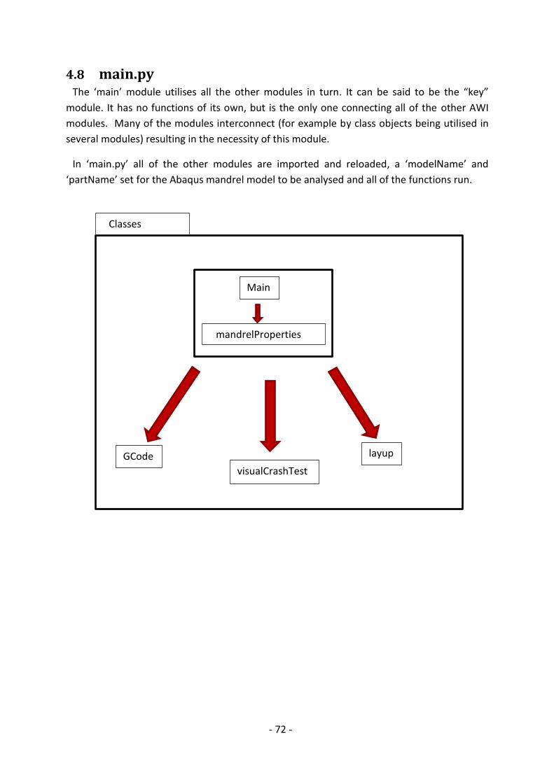
- 72 -
4.8 main.py The ‘main’ module utilises all the other modules in turn. It can be said to be the “key”
module. It has no functions of its own, but is the only one connecting all of the other AWI
modules. Many of the modules interconnect (for example by class objects being utilised in
several modules) resulting in the necessity of this module.
In ‘main.py’ all of the other modules are imported and reloaded, a ‘modelName’ and
‘partName’ set for the Abaqus mandrel model to be analysed and all of the functions run.
mandrelProperties
Main
GCode
visualCrashTest
layup
Classes

- 73 -

- 74 -
5. Evaluation
This thesis has been a pilot study and the modules developed are intended to serve as a
basis for further development. The contents of this chapter are intended to aid whoever will
continue the work in the future. It poses questions regarding the current modules and
suggests opportunities for further work that might be beneficial in a start-up process.
5.1 General Notes The modules have all been tested on Abaqus mandrel models with different types of mesh
and spatial orientations. However, all of these models are quite small and, with one
exception, have fairly large elements. As a precaution a test model should be created with a
large cylinder radius and very small elements. This will ensure that there are no problems
with the functions when the elements grow smaller.
It should also be investigated whether it is possible to have the module files located in a
different directory than the Abaqus work directory. As the AWI software grows it will
become impractical to have all the files in the Abaqus work directory instead of in a separate
AWI directory.
5.2 Remarks on Existing Functions This section discusses possibilities of improvement and expansion of the current AWI
modules.
5.2.1 Classes.py
5.2.1.1 MachineParameters
This class currently only allows for the parameter composition of the filament winding
machine at NTNU, which is a five-axis machine. It might be beneficial to expand the class, to
create functions for other types of machines as well, with different number of axes.
Another practical functionality, would be the possibility to store a set of machine
parameters or a ‘machineParameters’ object. Such a function would negate the need to
insert the same machine parameters every time the software is used. This functionality
would be especially beneficial if the software is used to generate CNC programs for more
than one filament winding machine.
Chapter

- 75 -
Lastly, a function for converting units from inches to millimetres would increase the
flexibility of the software even more. This is no difficult task to do by hand, but it is an added
luxury for whoever is using the software if the manual conversion is rendered unnecessary.
5.2.1.2 CylindricalMandrel
The mandrel is currently one of the most restricting factors of the AWI software, and one
of the key variables in filament winding. It is, therefore, an aspect of the software that
should be made more flexible.
There are numerous possibilities for how additional mandrel shapes could be
implemented. Additional mandrel classes could be created, or the current mandrel class
could be changed to allow for different types of mandrels. Possibly, the mandrel class could
be changed to contain shapes that can be combined (cylinder, cone, elliptical dome,
spherical dome etc.), instead of predefined mandrel compositions. No matter the mode,
there should be options for any type of mandrels; Both cylindrical and conical mandrel, with
elliptical, spherical or parabolic dome shapes should be possible.
Furthermore, it could be beneficial to implement a function that can create a standard
Abaqus mandrel model based on manual input parameters from the GUI. With such a
function the user would be given the opportunity to choose between a custom mandrel
created in Abaqus or one of several standard mandrels already stored in the software. A
simple GUI could be created for input of geometrical variables, with several standard profiles
available. Depending on the needs of the user, the appropriate combination of cylinder
shapes, dome shapes and radii would be chosen.
Currently the ‘verifyMandrel’ function only prints a statement in the Abaqus Message Area
if the mandrel exceeds the limitations of the filament winding machine. It does not in any
way disrupt the running of the modules. A possible way to deal with this would be to create
an exception class for mandrel values that are too great, and then interrupt the modules.
5.2.1.3 Material
The material class could easily be expanded by adding further standard materials. In
addition it should contain a function to create a custom material with unique material
properties in case this should be needed.
5.2.1.4 CNCLine
In this class the rounding of the CNC block variables is performed. To minimise the
numerical errors caused by this procedure an additional variable for the machine tolerance
could be added. This way there would be no additional numerical errors caused by the
function, outside of those already present.
The class could also be made to include additional types of CNC blocks; like modal
command lines or comments. This would create added flexibility to the software, making it
able to, for example, choose the modal commands to be included.

- 76 -
5.2.1.5 GCode
This function adds the topmost lines to a generated CNC program, but does not include any
kind of calculation of the point of origin for the winding in relation to the filament winding
machine. In other words: it assumes the feed-eye of the filament winding machine to be
located at the tip of the mandrel. There should be an additional parameter (for example in
this class or the ‘machineParameters’ class), that includes the distance from the winding
machine point of origin to a point on the mandrel. This distance should then be taken into
account when generating the CNC program.
Aside from these small facts, the main thing that needs to be done about this function is to
implement the kinematic equations for a filament winding machine. This is one of the key
concepts of the software, and should be prioritised. One possible approach to the problem
could be to form a collaborative group, including someone with a deeper understanding of
automation in the filament winding process.
5.2.2 MandrelProperties.py
5.2.2.1 determineRotationalAxis
In this function it was deemed necessary to round the radii variables to make the function
work. Although, as previously mentioned, this has no adverse effects on any calculations, the
necessity of the ‘round(…)’ function should be investigated. If the hypothesis posed in
chapter 4.4.2.2 is correct, it should not pose a problem. However, as the issue could be
caused by other factors, it might affect the software in unknown ways. This is especially true
as so many of the modules rely heavily on nodes and nodal coordinates.
With a fail-safe in place it is highly unlikely that this ‘round’ function will cause a false
positive. This has, however, not been tested for extremely small meshes. A test model
should be created, and the effects of a small mesh size investigated. It might be that this,
combined with the ‘round’ function, will result in false positives despite the fail-safe.
The ‘determineRotationalAxis’ function should also be expanded to include functionalities
for different types of mandrel shapes. Currently, it is based on a cylindrical mandrel with
spherical domes, and requires that a part of the mandrel is cylindrical to work. If the mandrel
shape is conical, the two elements compared must be located next to each other around the
circumference of the mandrel for the function to work. The mesh elements might be placed
randomly, and there is therefore no guarantee that this function will work for such a
mandrel. There is, of course, a small chance that it will work, but leaving it up to chance
whether a function works or not is far from ideal.
As the software is developed and expanded to include different types of mandrels (not only
conical, but also elliptical or square are possibilities) it should be investigated whether this
approach is the best one, or if an alternative approach ought to be found. It might be that
the best way to determine the rotational axis is to tailor functions to each mandrel type, or
some other way as of yet conceived.

- 77 -
5.2.2.2 determineRadii
The efficiency of this approach should be investigated. There are grounds for debating
whether the ‘determineRadii’ function is as efficient as it could be. The function iterates
through all of the nodes of every element. This means that in reality, depending on mesh
type, each node is investigated three or four times. If one wishes to keep the tools functional
for every type of mesh, this might prove a challenge. With no way to predict the element
and node placements it is not possible to, for example, exclude a certain set of nodes off
hand. One possible solution could be to register the investigated nodes in a list or a class and
then check whether the current node has already been used. It is, however, unlikely that this
will actually be more efficient than the current solution.
One viable solution would be to use the ‘getByBoundingBox(…)’ command to collect a
selection of elements along the axis of rotation. The command has no required arguments,
which means that if no boundaries are given in any one direction the bounding box will be
infinite in that direction. Knowing the rotational axis, this can be utilised by creating a box
that is infinite along the axis of rotation. The rest of the variables need to be determined
somehow, as the spatial orientation, except for the rotational axis, is unknown. It is
important that they are chosen in such a way that elements on all parts of the mandrel are
included. Figure 33 shows black bounding boxes encompassing elements of all radii, while
the red bounding box does not.
Figure 33 - Bounding box on mandrel

- 78 -
One suggestion on how to do this is written using pseudo code below.
#choosing the proper limits for the boundingBox
if (mandrel.rotationalAxis == X_AXIS):
boxY = boxZ = maxBox = None
numVar = 0
while not maxBox:
numVar += 10
boxY = mandrel.elements.getByBoundingBox(
yMin = -1*numVar
yMax = numVar)
boxZ = mandrel.elements.getByBoundingBox(
zMin = -1*numVar
zMax = numVar)
if (len(boxZ) > len(boxY)):
maxBox = boxZ
else:
maxBox = boxY
After the elements have been properly chosen, the current ‘determineRadii’ function can
be used. There will still be unnecessary iterations, but not nearly as many as in the present
version. the number of elements will have been greatly reduced, thereby greatly increasing
the efficiency of the function.
This method is based on the premise that the part sketch is done in a plane of the global
coordinate system. Seeing as how the rotational axis has to correspond to one of the global
axes it is considered implausible that this is the case. Should it be a cause for worry a
solution should not prove too challenging to implement. Using trigonometry it should prove
simple to write a function incrementally rotates the bounding box until elements have been
gathered. In addition, the current function, iterating through all of the elements, could be
used as a fail-safe.
5.2.2.3 determineLength
This function works in the exact same way as the ‘determineRadii’ function, and, as such,
has the same weaknesses. Most of the nodes are investigated several times, but the
problem can be solved in the same way as for the above-mentioned function.
For a cylindrical mandrel it will not always be considered necessary to model the entire
length of the mandrel. The dome and its shape are more important factors, and the proper
cylinder length can easily be simulated for analysis. For such cases it might be convenient to
implement an option for manual input of the true cylinder length.

- 79 -
5.2.3 GCode.py
5.2.3.1 createCNCProgram
The initial lines of the CNC program are set upon initiation of the ‘GCode’ class. It should be
considered, however, whether to include an additional line that moves the feed-eye to the
start position, and then stops, so that the fibres can be attached to the mandrel. If there is
no such function in the CNC program the fibres must be attached before the program is run.
As the feed-eye might have to move far before the winding can start it might cause problems
during wet winding. Fibres, already impregnated, are likely to cause a mess in such
situations.
It has been observed that at least some CNC programs are written with ‘,’ as the decimal
point, in Abaqus floats use ‘.’ as their decimal points. It should be investigated what the
standard is and how it can be determined, then a function written accordingly.
5.2.4 layup.py
5.2.4.1 collectLayupElements
The assumption for this function is that the geodesic curve on a cylinder projected onto a
plane can be approximated to a straight line. As shown in D.3 this is only true under
certain conditions. It should therefore be investigated whether it is possible to use the
parametric functions of a helix more directly to determine the winding path in the plane.
This would, most likely, result in a more flexible function capable of handling several
different shapes.
In addition, there are currently conditions for the points, ‘P1’ and ‘P2’, of the CNC program
block. They should located in the same quadrant or adjoining quadrants, and the two points
cannot be too close to the relevant axes (horizontal axis for ‘P1’ in quadrants I and III, and
vertical axis for ‘P1’ in quadrants II and IV). These conditions are, however, not enforced.
There is no test verifying that the conditions are actually fulfilled. Such a test should be
implemented, including measures to take if the test fails. For example, the movement could
be split into two smaller portions if the angle between the points is too great, or if one or
both are located too close to the horizontal or vertical axis.
Lastly, it should be investigated whether this approach is sound across the mandrel dome.
Currently, the assumption is that the movements along the axis of rotation across the dome
are small. With small movements it is possible to approximate the dome segment to a
cylinder with a certain numerical error. It is unlikely that this holds, especially towards the
tip of the dome, and an alternative solution should be found.

- 80 -
5.2.4.2 addLayup
For the ‘input from file’ mode of operation for this function it is most likely possible to
insert the complete file path for the CNC program file. This would negate the need of
copying the file into the Abaqus work directory. This has, as of yet, not been tested, but
should not prove too challenging to determine and implement.
An interesting extension for this module would be to include the fibre bandwidth in the
calculations. It should be investigated whether it is possible to include this parameter into
the mathematical method determining the elements on which to add layup. Instead of just
investigating whether the line between ‘P1’ and ‘P2’ crosses an element, one could include a
distance +/- half the bandwidth as well.
Another possibility for creating an accurate winding layup would be to section the actual
part instead of an ‘Orphan Mesh Part’. This would be more accurate in terms of shape and
path, but also more complex in its approach. Amongst others, the location of the pathway
on the model would need to be determined and a generic way of sectioning the part
according to the pathway, winding angle and bandwidth created to use in a script.
Challenges with this module include some of the assumptions made about the filament
winding machine. It assumes that any and all winding programs originate at the tip of the
mandrel dome. This is something that must be investigated further. There is no set standard
for this variable, and it might change depending on the software used to generate the
winding program. It should be determined whether there is any kind of set standard or
norm, what is the most typical starting point for winding software and if there is any way to
know this by checking the code or some kind of software manual.
Also, the axis designations are assumed to correspond to the filament winding machine at
NTNU, which might not always be the case. As the AWI software is expanded, a way needs to
be found to account for possible differences in axis designations of the winding machine and
the CNC program. A verification script needs to be written, ensuring that the values
extracted and set are indeed the values they are assumed to be; for example that the ‘X’
value does in fact describe the rotation of the mandrel.
Currently the tool assumes incremental movement of the filament winding machine. This is
the most common setting, but there is no guarantee that a CNC program is not written using
absolute dimensioning. It would be fairly simple to check this variable using Python regular
expressions on the program block containing modal commands.

- 81 -
This module relies heavily on the Abaqus ‘getByBoundingBox’ command. In using this
command it is important to note that the bounding box must envelop complete elements for
them to be collected. Figure 34 shows a mandrel part with a bounding box in red, and four
shaded elements that are collected in the box. If the mandrel elements are too great, or the
steps of the CNC block too small, no elements will be collected. This has the potential to
greatly affect the accuracy of the resulting winding layup.
Some kind of functionality should be implemented to handle such cases, when the
‘collectBoxElements’ function returns an empty list. One possibility, would be to store the
‘minCoords’ and ‘maxCoords’ lists in-between steps, for example in the ‘ConstructionLayup’
object. ‘minCoords’ and ‘maxCoords’ for the two steps could then be compared and a bigger
bounding box generated. Should the ‘collectBoxElements’, once again, return an empty list,
the process can be repeated and the second set of ‘minCoords’ and ‘maxCoords’
overwritten.
This module adds a unique composite layup, with a unique set of plies, to each element.
Due to the way the function collects the layup elements, and the approximations, there is
currently no guaranteeing that the elements have the same number of plies. Also, the angle
on each ply might not correspond the way they are supposed to, for example if there is a
“missing” ply. It has not been investigated how Abaqus calculates stresses in a composite
layup during analysis. Therefore, documentation should be found on this subject, and the
function changed, to ensure that it will truly render the desired result of an accurate
filament winding layup. The fibres used in filament winding are continuous, and the finished
Abaqus mandrel model should reflect that fact before it is analysed.
Although the approximation is a very good one it has not been investigated whether it does
actually correspond to the physical attributes of a real part. It should be checked whether
only a part of the mandrel being model has any bearing on the results. As the winding layups
are unique for each element the part cannot be said to be symmetrical, but it might prove to
Figure 34 - collecting elements by bounding box

- 82 -
be close enough to symmetrical to be acceptable. If this turns out not to be the case one
solution would be to automatically model a part with the same parameters as the partial
model, or to complete the partial model by revolving and mirroring the existing part.
Currently, the module has only been tested for arbitrary P1 values on different mandrel
models, and not for a complete CNC program. It is possible that using a proper CNC program
will result in unforeseen problems that need to be dealt with.
5.2.5 visualCrashTest.py
At the moment this module only supports movement extracted from the ‘lines’ variable of
a ‘CylindricalMandrel’ object. Using the same approach as the ‘layup’ module this script
could probably be updated to include functionality to run a visual crash test based on a CNC
program file, as well as the generated CNC program.

- 83 -
5.3 Further Expansions In this section suggestions are made for some additional modules and their hypothetical
properties.
5.3.1 Graphical User Interface (GUI)
As the software grows it will also become more complex and unmanageable. It will be
difficult to keep track of all of the functionalities, variations and permutations embedded in
the software. The code structure is likely to become less structured and more confusing for
those not intimately familiar with it. The simple solution is to create a software GUI from
which operations and functionalities are run. A GUI helps section functions into a more
apparent structure. It will make it easier to get started for new users, as well as eliminate the
need to be familiar with Python and programming to use the software.
Lastly, a GUI might also help spreading the software. As the intention is for the modules to
be universal, flexible and that those using them should continue the development, it is
imperative that they are considered worthwhile to learn and improve. With a GUI it is more
likely that new users, unfamiliar with the software, will take the time to familiarise
themselves with it.
5.3.2 Winding Parameters
As briefly mentioned in chapter 2.1 there are numerous parameters that affect the
mechanical properties of a filament wound part. Cross-over points, feed-rate, thickness
build-up and fibre tension are just some of these. An investigative study should be done,
defining and sorting these parameters, and determining how they can be implemented in
the software. This should be done, not only in terms of generating a CNC program, but also
in terms of modelling in Abaqus. Studying how Abaqus models and analyses composite layup
should be an important part of optimising the AWI software.
5.3.3 Circumventing the Abaqus GUI
Currently this software works though the Abaqus GUI. However, for some of the modules
this is not technically necessary. For example, there is no need for the GUI when determining
the mandrel properties. As long as the model name and part name are known, the module
can be run without the need for a viewport. As mentioned in chapter 2.3.2 there is a way of
communicating with the Abaqus kernel, without the use of the GUI. It might be beneficial to
investigate how this is done, and whether it would be practical to implement such
functionality. Most likely, as the software expands, there will be more modules not
dependent on the Abaqus GUI, and as an AWI GUI is created it might be considered
impractical to have both GUIs running at once.

- 84 -
6. Conclusion
This thesis has been a pilot study into the development of filament winding software
capable of integrating with FEA software. The goal was to create the basis for highly flexible,
open source software from which development might be continued. Key functionalities of
the software were to be generation of a CNC program for a part modelled in Abaqus, and the
addition of a corresponding, accurate composite layup to the modelled part.
Much to the surprise of this author and her supervisor both, the documentation of the
kinematics of filament winding were not as thorough and easily accessible as initially
presumed. After an extensive literature study only five papers were found on the subject, all
of which, for various reasons, were dismissed. What was to be a big part of the thesis
groundwork was therefore determined to be outside of the thesis scope. Instead, focus was
shifted entirely to the software development.
To produce software adequately flexible and comprehensive it was decided that attention
must be paid to the structure, readability, and simplicity of the code, and to generally sound
and thorough reasoning when creating the framework. The intention being that others can
continue the development process independently of the author, without aid. As the
software is completely open source, the aim is that anyone and everyone using the software
solution can add on to, change and optimise the functionalities according to their specific
needs. Such continuous expansion and bettering of the software would ensure it being up to
date, always improving.
The primary result of this thesis is the “Abaqus Winding Integration” (AWI) software
solution. It is a set of modules with several different functionalities related to filament
winding. Those functionalities include extracting mandrel properties from an Abaqus
mandrel model of a cylindrical part with spherical domes, and a framework for the
generation of a CNC program for that same model. The AWI software includes functionalities
for performing a visual simulation of the winding process in the Abaqus GUI based on a
generated CNC program. Finally, it also includes a module for adding a composite layup to an
Abaqus mandrel model. The layup will correspond directly to a CNC program generated
using the AWI software, or to a CNC program imported from an external file; it generates an
accurate model for the filament wound part on which analysis can be performed.
Chapter

- 85 -
6.1 Further Work The following is a summary of the discussion in chapter 0 – Evaluation. Recommendations
are made for those who are to continue the development to investigate the following areas:
o The kinematics of filament winding need to be investigated and understood.
o The AWI software should be expanded to include several additional types of mandrel
and dome combinations.
o A GUI should be developed and implemented.
o The layup module should be expanded and the mathematical method perfected.
o The winding parameters influencing filament winding should be mapped and a plan
of implementation made
In addition to the abovementioned main areas sever smaller suggestions were made
(function converting from millimetres to inches, additional choices for type of filament
winding machine, reading and adding modular G codes, a more effective ‘determineRadii’
and ‘determineLength’ functions, etc.)

- 86 -
Bibliography 1. Cadwind Features. Material; Available from:
http://www.material.be/cadwind/features/index.html. 2. Winding Expert. Mikrosam; Available from:
http://www.mikrosam.com/new/article/en/winding-expert/. 3. Press Release from Seifert & Skinner. ComposicaD; Available from:
http://www.seifert-skinner.com/Other/PressReleaseJuly2010.pdf. 4. Abaqus Extension for Filament Wound Composite Structures, Capability Brief. Simulia;
Available from: http://www.simulia.com/products/extensions/AppBrief_COPV.pdf. 5. Peters, S.T., Composite filament winding2011, Materials Park, Ohio: ASM
International. VI, 167 s. 6. Seereeram, S. and J.T.Y. Wen, An all-geodesic algorithm for filament winding of a T-
shaped form. Industrial Electronics, IEEE Transactions on, 1991. 38(6): p. 484-490. 7. Peters, S.T., W.D. Humphrey, and R.F. Foral, Filament winding composite structure
fabrication1999, Covina, Calif.: SAMPE International Business Office. Div. pag. 8. Lubin, G., Handbook of fiberglass and advanced plastics composites1969, New York:
Van Nostrand Reinhold. XVIII, 894 s. 9. Eckold, G., Design and manufacture of composite structures1994, Cambridge:
Woodhead. VIII, 397 s. 10. Shen, F.C., A filament-wound structure technology overview. Materials Chemistry and
Physics, 1995. 42(2): p. 96-100. 11. Green, J.E., Overview of filament winding. SAMPE Journal, 2001. 37(1): p. 7-11. 12. Company. Material; Available from: http://www.material.be/company/index.html. 13. Cadwind Demo and tutorial downloads. Material; Available from:
http://www.material.be/cadwind/download/index.html. 14. Mikrosam history. Mikrosam; Available from:
http://www.mikrosam.com/new/article/en/history/. 15. About ComposicaD. ComposicaD; Available from:
http://www.composicad.com/about.php. 16. ComposicaD flyer. ComposicaD; Available from:
http://www.composicad.com/ComposiCAD_Flyer1.pdf. 17. About SIMULIA. Simulia; Available from: http://www.abacom.de/about/about.html. 18. Abaqus FEA. Simulia; Available from:
http://www.abacom.de/products/abaqus_fea.html. 19. Abaqus/CAE. Simulia; Available from:
http://www.abacom.de/products/abaqus_cae.html. 20. Composite Filament Winding, Abaqus. Simulia; Available from:
http://www.simulia.com/products/wound_composites.html. 21. Python. Available from: www.python.org. 22. Python Standard Libraries 23. Simulia, Abaqus Scripting User's Manual. Abaqus Documentation, 2010. 24. Simulia, Abaqus Scripting Reference Manual, 2010. 25. Smid, P., CNC programming handbook: a comprehensive guide to practical CNC
programming2003, New York: Industrial Press. XX, 508 s. 26. Abdel-Hady, F., Filament winding of revolution structures. Journal of Reinforced
Plastics and Composites, 2005. 24(8): p. 855-868.

- 87 -
27. Trajkovski, D., Kinematic Analysis of Trajectory Generation Algorithms for Filament Winding Machines. Proceedings of the 11th World Congress in Mechanism and Machine Science, 2003.
28. Koussios, S., Filament Winding a Unified Approach, 2004, Delft University of Technology.
29. Koussios, S., O.K. Bergsma, and A. Beukers, Filament winding. Part 2: generic kinematic model and its solutions. Composites Part A: Applied Science and Manufacturing, 2004. 35(2): p. 197-212.
30. Koussios, S., O.K. Bergsma, and A. Beukers, Filament winding. Part 1: determination of the wound body related parameters. Composites Part A: Applied Science and Manufacturing, 2004. 35(2): p. 181-195.
31. Maple webpages. MapleSoft; Available from: http://www.maplesoft.com/products/maple/index.aspx.
32. Python Regular Expressions1. Python; Available from: http://docs.python.org/library/re.html.
33. Python Regular Expressions2. Python; Available from: http://docs.python.org/howto/regex.html.
34. Helix. Wolfram Alpha; Available from: http://www.wolframalpha.com/input/?i=helix. 35. Cutting Helix. Wolfram Alpha; Available from:
http://mathworld.wolfram.com/Helix.html.

A-1
Appendix A – List of Figures
Figure 1 - Filament winding of cylindrical mandrel with domes ......................................... - 3 -
Figure 2 - Simulated elbow winding pattern [1] .................................................................. - 4 -
Figure 3 - Geodesic t-shape winding pattern [6] ................................................................. - 4 -
Figure 4 – Polar and helical winding patterns [5] ................................................................ - 6 -
Figure 5 – Cadwind [1] ......................................................................................................... - 8 -
Figure 6 - Winding Expert [2] ............................................................................................... - 9 -
Figure 7 – ComposicaD [3] ................................................................................................. - 10 -
Figure 8 - Abaqus user interface ........................................................................................ - 11 -
Figure 9 - Wound Composite Modeler [4] ......................................................................... - 12 -
Figure 10 - Abaqus scripting interface commands and Abaqus /CAE ............................... - 14 -
Figure 11 - Abaqus structure.............................................................................................. - 16 -
Figure 12 - 'models' object ................................................................................................. - 17 -
Figure 13 - Elements and nodes ......................................................................................... - 17 -
Figure 14 - Python print function ....................................................................................... - 18 -
Figure 15 - CNC example .................................................................................................... - 20 -
Figure 16 – Absolute dimensioning ................................................................................... - 22 -
Figure 17 - Incremental dimensioning ............................................................................... - 22 -
Figure 18 - Fibre paths ....................................................................................................... - 28 -
Figure 19 - Mandrel and 'Orphan Mesh Part' .................................................................... - 34 -
Figure 20 - Structured mesh .............................................................................................. - 35 -
Figure 21 - Unstructured mesh .......................................................................................... - 35 -
Figure 22 - Axis configurations ........................................................................................... - 37 -
Figure 23 – Mandrel properties ......................................................................................... - 37 -
Figure 24 - Different radii for a node ................................................................................. - 40 -
Figure 25 - GCode opening lines ........................................................................................ - 42 -
Figure 26 - Placement of P2 ............................................................................................... - 43 -
Figure 27 - Node returning wrong radius .......................................................................... - 47 -
Figure 28 – Simplified problem .......................................................................................... - 56 -
Figure 29 - Bounding box between P1 and P2 ................................................................... - 60 -
Figure 30 - Projection of elements ..................................................................................... - 62 -
Figure 31 - Straight line crossing element ......................................................................... - 63 -
Figure 32 - Mandrel and feed-eye assembly ..................................................................... - 69 -
Figure 33 - Bounding box on mandrel ............................................................................... - 77 -
Figure 34 - collecting elements by bounding box .............................................................. - 81 -
Figure 35 - Sphere ................................................................................................................ D-1
Figure 36 - P1 in quadrant I .................................................................................................. D-2
Figure 37 - P1 in quadrant II ................................................................................................. D-2
Figure 38 - P1 in quadrant III ................................................................................................ D-2

A-2
Figure 39 - P1 in quadrant IV ............................................................................................... D-2
Figure 40 - plot of x(t), z(t) for R = 20, c = 1 ......................................................................... D-4
Figure 41 - Projected element and winding path ................................................................ D-5
Figure 42 - Helical path on cylinder ..................................................................................... D-6
Figure 43 - Circle segment on cylinder ................................................................................ D-6

B-1
Appendix B – Research History During the literature study the scientific article databases Scopus, Elsevier, EI Village and
google scholar were used.
As a point of origin for the literature study the paper “Filament Winding of Revolution
Structures” by Faissal Abdel-Hady was used [25]. This paper was used as a main source in a
previous project, but was shown to contain several mistakes and therefore considered
unreliable. With one exception it proved almost impossible to find the sources cited in the
abovementioned article. Instead it was decided to use the articles citing this one instead, a
functionality which can be found in most of the article databases. There were five such
articles. From this point of origin a thorough investigation of these articles, their sources,
their sources’ sources and so on was done.
In addition a search using the following search words was conducted.
- “Filament Winding” automation
- Geodesic path algorithm
- Determination of Feed-eye Position
- Algorithm “filament winding”
- Machine Control “filament Winding”
- (feed-eye pay-out eye) (movement algorithm)
At one point there were no new articles, books or related books. The decision was made
that, although scarce, the documentation found should suffice.

C-2
Appendix C – Evaluation of Equations This appendix details the mathematical inconsistencies of “Filament Winding of Revolution
Structures”, by Faissal Abdel-Hady [25].
The equations given in the paper are as follows:
0
'
0
2'
0
sintan
R cosR
1 R
(2)
'
0
'
0
0 02
R cos cosx R sin sin
1 R
(3)
0
0' 2
cosz z
1 R
(4)
' '
0 0
2
costan
R sin sin 1 R cos sin
(5)
In the derivation of equations (2) through (4) the two following equations are utilised:
'
0
'
0
'
0
'
0
'
2
2
2
0
R cos cossin sin
1 R
R sin sinT cos sin
1 R
cos
1 R
(28)
0 0
0
0
R cos x
T R sin
z z
(29)
Following the logical steps in combining equations (28) and (29) equation (2) remains the
same, but equations (3) and (4) suffer minor changes. In equation (3) the first term of the
equation r should be r cos , and the sign of the last term of equation (4) should be the
opposite.

C-3
In the derivation of equation (5) three equations are utilised:
n T xf x (30)
x x i (31)
'
0
'
0
'
0
'
0
'
2
2
2
0
R cos cossin sin
1 R
R sin sinT cos cos
1 R
cos
1 R
(32)
Combining equations (30), (31) and (32), supposedly result in equation (33)
'
0
'
0
'
0
f2
2
0
cosn
1 R
R sin sincos cos
1 R
(33)
Upon close inspection, however, it can be seen that the two equations (28) and (32),
although expressions for the same variable, are not identical. Regardless of which of the two
are used to derive equation (33), it is not correct. Looking at equation (5) it is assumed that
equation (28) is the correct one. Accurately making use of the vector product of (28) and
(31) equation (33) should be:
'
0
'
0
'
2
2
0
f
0
cosn
1 R
R sin sincos sin
1 R
(34)

C-4
Accordingly equation (5) should read:
2
2
2
'
f j 0
'f k 0
'
0
' '
0 0
cos
n 1 Rtan
n R sin sincos sin
1 R
cos
R sin sin 1 R cos sin
(35)

D-1
Appendix D – Derivation of Equations This appendix contains derivation of formulae used in the Abaqus Winding Integration
tools.
D.1 Mandrel Length Equation (36) describes any point on the surface of a sphere in Cartesian coordinates.
2 2 2 2R x y z (36)
Any cross-section in the xz-plane (marked in red on Figure 35) will be a circle for which the
following holds:
2
d
2 2r x z (37)
Combining equations (36) and (37) yields equation for the y coordinate of the point ‘P’ in
terms of the radius of the sphere, ‘R’, and the radius at point ‘P’, ‘r’.
2 2y R r (38)
Figure 35 - Sphere
Equation (38) describes the length of a mandrel dome in terms of the dome radius, ‘r’, and
the cylinder radius, ‘R’. Adding up with the length of half a cylinder this yields the equation
for the true length of a cylindrical mandrel with spherical domes:
2 2mandrelLength 2 R r cylinderLength
(15)
P
Y
X
Origin (0, 0, 0) rd
Z

D-2
D.2 Coordinates of P2 This approach is based on ‘P1’ being located in one of the quadrants of the unit circle, and
‘P2’ being located in the same, or adjoining, quadrant. Figure 36 through Figure 39 show ‘P1’
in different quadrants and the respective possible locations of ‘P2’.
P2
P2 V
H
IV III
I II
X
W W
X
U
P1
P2
P2
V
H
IV III
I II
X W
W
X
U
P1
Figure 36 - P1 in quadrant I Figure 37 - P1 in quadrant II
P2 P2
V
H
IV III
I II
X
W W
X
U
P1
P2
P2
V
H
IV III
I II
X
W
W
X U
P1
Figure 39 - P1 in quadrant IV Figure 38 - P1 in quadrant III
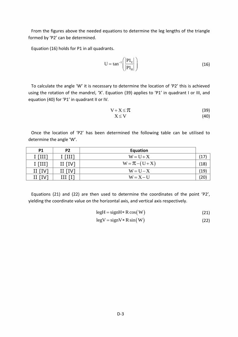
D-3
From the figures above the needed equations to determine the leg lengths of the triangle
formed by ‘P2’ can be determined.
Equation (16) holds for P1 in all quadrants.
V1
H
P1U tan
P1
(16)
To calculate the angle ‘W’ it is necessary to determine the location of ‘P2’ this is achieved
using the rotation of the mandrel, ‘X’. Equation (39) applies to ‘P1’ in quadrant I or III, and
equation (40) for ‘P1’ in quadrant II or IV.
V X (39) X V (40)
Once the location of ‘P2’ has been determined the following table can be utilised to
determine the angle ‘W’.
P1 P2 Equation
I [III] I [III] W U X (17)
I [III] II [IV] W U X (18)
II [IV] II [IV] W U X (19)
II [IV] III [I] W X U (20)
Equations (21) and (22) are then used to determine the coordinates of the point ‘P2’,
yielding the coordinate value on the horizontal axis, and vertical axis respectively.
legH signH R cos W (21)
legV signV R sin W (22)

D-4
D.3 Linear Equations The parametric equations for a geodesic curve around a cylinder are as follows [33].
z(t) R cos(t) (41)
x(t) Rsin(t) (42)
y(t) ct (43)
Projecting the curve into the plane yields the curve depicted in Figure 40 for R = 20 and c =
1. Plotting in the yz-plane would result in the cosine curve.
From Figure 40 it is clear that as long as P1x and P2x are not too close to the radial value,
and they are located in adjoining quadrants, the path can be considered linear between two
points. The linear equation for such a line can easily be derived from the coordinates of
those two points. With this line in place the elements can be projected into the same plane
and it can be determined whether each element lies in the winding path or not.
Equations (23) and (24) are expressions for the straight line between two points.
y(x) xa b (23)
yx(y)
b
a
(24)
Figure 40 - plot of x(t), z(t) for R = 20, c = 1

D-5
With two known points P1(x1, y1) and P2(x2, y2) the slope variable, ‘a’, and constant, ‘b’,
can be calculated using equations (25) and (26).
2 1
2 1
y y
x xa
(25)
1 1y xb a (26)
Knowing the nodal coordinates of an element it can easily be projected onto the same
plane as the line between ‘P1’ and ‘P2’. To ascertain whether the element is in the winding
path it must be determined if a point of the line lies between the boundary values of the
element. This has been illustrated in Figure 41.
Figure 41 - Projected element and winding path
The right square in Figure 41 shows an element in the winding path. Inserting the element
‘minX’ value in equation (23) yields the cross-over point between the winding path and the
left hand vertical element boundary. The element ‘maxY’ value in equation (24) yields the
cross-over point between the winding path and the topmost horizontal element boundary.
The cross-over values will be between the minimum and maximum values of their respective
axes. If the values are not between the minimum and maximum values the element is not in
the winding path.
y
x
Projected element:
maxY
minY
min
X
maxX
Element not in winding path:
P1
P2
P2
Element in winding path:
P1

D-6
D.4 Winding Angle, α
Figure 42 - Helical path on cylinder
If a cylinder with a helical pattern is cut and unfolded the resulting path on the resulting
rectangle is a straight line [34]. From Figure 42 it is clear that equation (44) must be true.
Ytan
s (44)
From Figure 43, and using the rules of ratio,
equation (45) is derived.
X 2 1
s 2 R R
(45)
Combining equations (44) and (45) results in equation (27); an expression for the winding
angle on a cylindrical mandrel in terms of the rotation of the mandrel, ‘X’, the lateral
movement along the axis of rotation, ‘Y’, and the radius of the cylinder, ‘R’.
Ytan
RX (27)
α
s
Y
X
s
P1 P2
Figure 43 - Circle segment on cylinder

E-1
Appendix E – Integration Tools Following are the Abaqus Winding Integration Tools in their entirety.
Note that the line numbers will not be identical to those in the *.py files as they have been
formatted slightly for this appendix.
E.1 classes.py################################################################# 1 # # 2 # CLASSSES # 3 # # 4 ################################################################# 5 6 ''' 7 This file contains all the classes used in 8 the Abaqus Winding Integration Tools 9 10 For more information about the functions, how they work and why 11 the procedures have been chosen see 12 "Integration Tools for Design and Process Control of Filament 13 Winding" 14 by Inger Skjaerholt 15 ''' 16 17 # necessary Python and Abaqus libraries and files 18 from abaqus import * 19 from abaqusConstants import * 20 21 import math 22 23 ### global constants. Do. NOT. Change. These! 24 X_AXIS = 0 25 Y_AXIS = 1 26 Z_AXIS = 2 27 28 ### BODY ### 29 ### Filament winding machine limits 30 class MachineParameters: 31 def __init__(self, string, maxMandrelRadius, maxWindingLength, 32 maxMandrelLength, maxZStroke, maxWStroke): 33 self.Name = string 34 ### machine parameters in mm 35 # parameters on X-axis 36 self.maxMandrelRadius = maxMandrelRadius 37 self.maxWindingLength = maxWindingLength #max length to wind 38 39 # parameters on Y-axis 40 self.maxMandrelLength = maxMandrelLength 41 #max length including shafts 42
43 self.maxZStroke = maxZStroke 44 self.maxWStroke = maxWStroke 45 46 47

E-2
### cylindrical mandrel with spherical end domes and with identical 48 dome openings 49 class CylindricalMandrel: 50 def __init__(self, modelName, partName): 51 # Model variables 52 self.modelName = modelName 53 self.partName = partName 54 self.model = mdb.models[modelName] 55 self.part = mdb.models[modelName].parts[partName] 56 self.nodes = mdb.models[modelName].parts[partName].nodes 57 self.elements = mdb.models[modelName] 58 .parts[partName].elements 59 60 # Geometrical variables 61 self.rotationalAxis = 'undetermined' 62 self.H = None #horizontal axis 63 self.V = None #vertical axis 64 self.radius = None 65 self.domeOpening = None 66 self.minLength = None 67 self.maxLength = None 68 self.mandrelLength = None #total length including domes 69 self.cylinderLength = None 70 self.pointOfOrigin = None 71 72 # G Code variables 73 self.lines = list() 74 self.domeVariable = 1 75 self.windingDirection = -1 76 77 ### Class functions 78 def setLength (self, minLength, maxLength): 79 self.minLength = minLength 80 self.maxLength = maxLength 81 self.cylinderLength = (maxLength - minLength) 82 83 self.calculateTotalLength() 84 self.setDomeVariable() 85 86 def calculateTotalLength(self): 87 self.mandrelLength = 2* ( 88 math.sqrt(self.radius**2 - self.domeOpening**2) 89 + 2*self.cylinderLength) 90 91 def setDomeVariable(self): 92 if (self.pointOfOrigin < self.minLength): 93 self.domeVariable = -1 94 95 # verifying that the mandrel does not exceed the capabilities of 96 the winding machine 97 def verifyMandrel (self, settings): 98 99 if (self.radius > settings.maxMandrelRadius): 100 print "The mandrel radius is too great for the ", 101 settings.Name, " machine" 102 103

E-3
if (self.mandrelLength > settings.maxWindingLength): 104 print "The mandrel length is too great for the ", 105 settings.Name, " machine" 106 107 else: 108 print "The mandrel is within the parameters of the ", 109 settings.Name, " machine" 110 111 def printProperties (self, settings): 112 self.verifyMandrel(settings) 113 print "Model: ", self.modelName, ", Part: ", self.partName 114 print "Rotational Axis: ", self.rotationalAxis 115 print "Radius: ", self.radius 116 print "Dome Opening: ", self.domeOpening 117 print "Length: ", self.cylinderLength 118 119 120 ### common winding materials 121 class Material: 122 def __init__(self): 123 self.Name = None 124 self.E_1 = None 125 self.E_2 = None 126 self.E_3 = None 127 self.nu_12 = None 128 self.nu_13 = None 129 self.nu_23 = None 130 self.G_12 = None 131 self.G_13 = None 132 self.G_23 = None 133 self.rho = None 134 self.thickness = None 135 136 def carbon_epoxy(self): 137 self.Name = 'Carbon_Epoxy' 138 self.E_1 = 14000 139 self.E_2 = 8000 140 self.E_3 = 8000 141 self.nu_12 = 0.3 142 self.nu_13 = 0.3 143 self.nu_23 = 0.55 144 self.G_12 = 4000 145 self.G_13 = 4000 146 self.G_23 = 2581 147 self.rho = 1600 148 self.thickness = 0.15 149 150 151 152

E-4
### often used node variables 153 class CustomNode: 154 def __init__(self, mandrel, element, node): 155 # nodal coordinate values 156 self.XYZ = [0, 0, 0] 157 self.XYZ[X_AXIS] = mandrel 158 .nodes[element.connectivity[node]].coordinates[X_AXIS] 159 self.XYZ[Y_AXIS] = mandrel 160 .nodes[element.connectivity[node]].coordinates[Y_AXIS] 161 self.XYZ[Z_AXIS] = mandrel 162 .nodes[element.connectivity[node]].coordinates[Z_AXIS] 163 164 # Radii calculated using different coordinate combinations 165 self.radii = [0, 0, 0] 166 self.radii[X_AXIS] = self.calculateRadius( 167 self.XYZ[Y_AXIS], self.XYZ[Z_AXIS]) 168 self.radii[Y_AXIS] = self.calculateRadius( 169 self.XYZ[X_AXIS], self.XYZ[Z_AXIS]) 170 self.radii[Z_AXIS] = self.calculateRadius( 171 self.XYZ[X_AXIS], self.XYZ[Y_AXIS]) 172 173 # calculate a radius using pythagoras 174 def calculateRadius (self, leg1, leg2): 175 return math.sqrt(leg1**2 + leg2**2) 176 177 # get the node radius 178 def returnRadius (self, rotationalAxis): 179 return self.radii[rotationalAxis] 180 181 # get the node coordinate ON the rotational axis 182 def returnAxisCoordinate(self, rotationalAxis): 183 return self.XYZ[rotationalAxis] 184 185 def printProperties (self, nodeName): 186 print nodeName, ':' 187 print 'XYZ = (', 188 self.XYZ[0], ' , ', self.XYZ[1], ', ', self.XYZ[2], ')' 189 print 'Radii = (', 190 self.radii[0], ' , ', self.radii[1], ', ', self.radii[2], ')' 191 192 ### CNC code line to be put in the mandrel variable 'lines' 193 class CNCLine: 194 def __init__(self, N, X, Y, Z, W): 195 self.N = N 196 self.X = X 197 self.Y = Y 198 self.Z = Z 199 self.W = W 200 201 self.string = "N{0} X{1} Y{2} Z{3} W{4}\n".format( 202 str(round(N, 5)), str(round(X, 5)), str(round(Y, 5)), 203 str(round(Z, 5)), str(round(W, 5))) 204 205 206 207

E-5
### G code variables 208 class GCode: 209 def __init__(self, filename, mandrel): 210 211 # increment variables 212 self.N = 10 #variable for the sequence number 213 self.increment = 10 #sequence number incremental value 214 215 # movement variables 216 self.totalX = 0 217 self.totalY = 0 218 self.totalZ = 0 219 self.totalW = 0 220 221 self.writeOpeningLines(filename, mandrel) 222 223 def writeOpeningLines(self, filename, mandrel): 224 self.GCodeFile = open(filename, 'w') 225 226 ### as the G-code file is created the topmost lines in the 227 program are written 228 # comment lines to explain for what type of mandrel the 229 program has been written 230 self.GCodeFile.write ( 231 '(This CNC program has been created using)\n') 232 self.GCodeFile.write ( 233 '(The Abaqus Winding Integration Tools)\n') 234 self.GCodeFile.write ('for a mandrel of:)\n') 235 self.GCodeFile.write ( 236 '(\tCylinder Radius: ' + 237 str(round(mandrel.radius, 2)) + ')\n') 238 self.GCodeFile.write ( 239 '(\tDome Opening: ' + 240 str(round(mandrel.domeOpening, 2)) + ')\n') 241 self.GCodeFile.write ( 242 '(\tCylinder Length: ' + 243 str(round(mandrel.cylinderLength, 2)) + ')\n') 244 self.GCodeFile.write ('\n\n\n') 245 246 # first block of the program with preparatory commands etc. 247 self.GCodeFile.write ('N10 G01 G21 G91 G94 F50000\n') 248 249 250

E-6
def addLine (self, settings, mandrel, X, Y, Z, W): 251 252 ### adding the movement to the total movement along the axes 253 self.totalX += X 254 self.totalY += Y 255 self.totalZ += Z 256 self.totalW += W 257 258 ### ensuring that the limits of the machine 259 have not been exceeded 260 if (self.totalY > settings.maxMandrelLength): 261 print "error! The maximum movement along the X-axis 262 has been exceeded" 263 264 if (self.totalZ > settings.maxZStroke): 265 print "error! The maximum movement along the Z-axis 266 has been exceeded" 267 268 if (self.totalW > settings.maxWStroke): 269 print "error! The maximum rotation around the W-axis 270 has been exceeded" 271 272 else: 273 # constructing the next line 274 self.N += self.increment 275 line = CNCLine (self.N, X, Y, Z, W) 276 277 # adding the line to the list of program lines 278 mandrel.lines.append(line) 279 280 # writing the line into the program file 281 self.GCodeFile.write(line.string) 282 return 283 284 # the limits of the machine have been exceeded 285 # the process is stopped 286 return "something to stop the loop" 287 288 289 290

E-7
### variables used while adding layup to a model 291 class LayupConstruction: 292 def __init__(self, P1): 293 # general variables 294 self.material = Material() 295 296 # movement variables 297 self.P1 = P1 #starting point for CNC block 298 self.P2 = [0, 0, 0] #ending point for CNC block 299 self.crossesHorizontal = False 300 self.crossesVertical = False 301 302 def printPoints(self): 303 print 'P1: (', 304 self.P1[0], ', ', self.P1[1], ', ', self.P1[2], ')' 305 print 'P2: (', 306 self.P2[0], ', ', self.P2[1], ', ', self.P2[2], ')' 307 308 309 ### Assembly with feed-eye 310 class Assembly: 311 def __init__(self, mandrel): 312 self.feedEye = 'Feed-Eye' 313 self.mandrelName = mandrel.modelName 314 self.assemblyDir = None 315 316 self.createFeedEye(mandrel) 317 318 def createFeedEye(self, mandrel): 319 # base sketch 320 sketch = mandrel.model.ConstrainedSketch ( 321 name = 'Section Sketch', sheetSize = 200.0) 322 323 sketch.CircleByCenterPerimeter((0.0, 0.0), (0.0, 5.0)) 324 325 # creating the part 326 part = mandrel.model.Part(name = self.feedEye) 327 part.BaseSolidExtrude (sketch = sketch, depth = 5.0) 328 329 def move (self, mandrel, Y, Z): 330 #using the axes of the FW machine at NTNU as a standard 331 # X = rotation of mandrel 332 # Y = movement along the rotational axis 333 # Z = movement perpendicular to the mandrel 334 # W = rotation of the feed-eye 335 336 # currently W and X are not relevant, 337 # but they will probably be in the future 338 339 newCoords = [0, 0, 0] 340 newCoords[mandrel.rotationalAxis] = Y 341 newCoords[mandrel.V] = -1*Z 342 343 self.assemblyDir.translate((self.feedEye, ), newCoords) 344 session.viewports['Viewport: 1'] 345 .view.setValues(drawImmediately = True)346

E-8
E.2 mandrelProperties.py################################################################# 1 # # 2 # FUNCTIONS TO DETERMINE MANDREL PROPERTIES # 3 # # 4 ################################################################# 5 6 ''' 7 This file contains functions to gather and set mandrel properties 8 based on a model from Abaqus/CAE 9 10 For more information about the functions, how they work and why 11 the procedures have been chosen see 12 "Integration Tools for Design and Process Control of Filament 13 Winding" 14 by Inger Skjaerholt 15 16 ''' 17 18 # necessary Python, Abaqus libraries and files 19 from abaqus import * 20 21 import classes 22 reload (classes) 23 24 ### global constants. Do. NOT. Change. These! 25 X_AXIS = 0 26 Y_AXIS = 1 27 Z_AXIS = 2 28 29 ### BODY ### 30 ''' 31 This function iterates through the list of mandrel elements 32 comparing radii in different directions to determine Rotational Axis 33 ''' 34 def determineRotationalAxis (mandrel): 35 counter = 0 36 element = mandrel.elements[counter] #first element in 37 the elements list 38 test = None #fail-safe test variable 39 40 currentNode = classes.CustomNode(mandrel, element, 0) 41 42 while mandrel.rotationalAxis == 'undetermined': 43 counter += 1 44 45 # if the counter has moved to the end of the elements list 46 # it was not possible to determine the rotational axis 47 if counter >= len(mandrel.elements): 48 print "it was not possible 49 to determine the rotational axis" 50 51 52

E-9
#ask for manual input through GUI 53 rotationalAxis = getInput( 54 'Enter the numerical value for the rotational Axis: 55 \n(X-Axis = 0, Y-Axis = 1, Z-Axis = 2)') 56 mandrel.rotationalAxis = int(rotationalAxis) 57 break 58 59 element = mandrel.elements[counter] #next element 60 nextNode = classes.CustomNode(mandrel, element, 0) 61 62 # if the coordinates are identical it is unnecessary to 63 compare them 64 if (currentNode.XYZ == nextNode.XYZ): 65 currentNode = nextNode 66 continue 67 68 ### comparing to see if the different radii are equal, 69 determining the rotational axis 70 if round(currentNode.radii[X_AXIS],5) == 71 round(nextNode.radii[X_AXIS], 5): 72 # if the fail-safe variable is 'None' or another axis 73 if test != X_AXIS: 74 test = X_AXIS 75 76 # if the previous comparison also returned this axis, 77 the rotational axis is set 78 elif test == X_AXIS: 79 mandrel.rotationalAxis = X_AXIS 80 mandrel.H = Z_AXIS 81 mandrel.V = Y_AXIS 82 83 if round(currentNode.radii[Y_AXIS], 5) == 84 round(nextNode.radii[Y_AXIS], 5): 85 if test != Y_AXIS: 86 test = Y_AXIS 87 88 elif test == Y_AXIS: 89 mandrel.rotationalAxis = Y_AXIS 90 mandrel.H = X_AXIS 91 mandrel.V = Z_AXIS 92 93 if round(currentNode.radii[Z_AXIS], 5) == 94 round(nextNode.radii[Z_AXIS], 5): 95 if test != Z_AXIS: 96 test = Z_AXIS 97 98 elif test == Z_AXIS: 99 mandrel.rotationalAxis = Z_AXIS 100 mandrel.H = Y_AXIS 101 mandrel.V = X_AXIS 102 103 104 # if the rotational axis has not been determined 105 move one element further 106 currentNode = nextNode 107 108

E-10
109 ''' 110 This function iterates through all the nodes on all the elements in 111 the elements list 112 determining the smallest and greatest radius along the axis of 113 rotation. 114 ''' 115 def determineRadii (mandrel): 116 minRadius = None 117 maxRadius = None 118 119 for element in mandrel.elements: 120 #number of nodes on an element. 121 Will vary depending on element type 122 nodesOnElement = len(element.connectivity) 123 124 # iterate through the nodes 125 for i in range(nodesOnElement): 126 currentNode = classes.CustomNode(mandrel, element, i) 127 128 # radius given by node j on element i 129 tempRadius = currentNode 130 .returnRadius(mandrel.rotationalAxis) 131 132 # set point of comparison on the first iteration 133 if minRadius == None: 134 minRadius = tempRadius 135 maxRadius = tempRadius 136 137 # in case the first node is on the dome opening 138 mandrel.pointOfOrigin = currentNode 139 .returnAxisCoordinate(mandrel.rotationalAxis) 140 141 elif tempRadius < minRadius: 142 minRadius = tempRadius 143 mandrel.pointOfOrigin = currentNode 144 .returnAxisCoordinate(mandrel.rotationalAxis) 145 146 147 elif tempRadius > maxRadius: 148 maxRadius = tempRadius 149 150 mandrel.radius = maxRadius 151 mandrel.domeOpening = minRadius 152 153 154 155

E-11
''' 156 This function iterates through all the elements in the elements list 157 determining the outer extreme coordinates on the rotational axis for 158 the cylinder 159 ''' 160 def determineLength (mandrel): 161 minLength = None#minimum coordinate value on the rotational axis 162 maxLength = None#maximum coordinate value on the rotational axis 163 164 for element in mandrel.elements: 165 # variable for the number of nodes on an element. 166 Will vary depending on element type 167 nodesOnElement = len(element.connectivity) 168 169 # iterate through the nodes 170 for i in range(nodesOnElement): 171 currentNode = classes.CustomNode(mandrel, element, i) 172 rotAxCoordinate = currentNode 173 .returnAxisCoordinate(mandrel.rotationalAxis) 174 tempRadius = currentNode 175 .returnRadius(mandrel.rotationalAxis) 176 177 # tempRadius is not equal to the cylinder radius 178 and therefore on the dome 179 if round(tempRadius, 5) != round(mandrel.radius, 5): 180 break 181 182 # set points of comparison on the first iteration 183 if minLength == None: 184 minLength = rotAxCoordinate 185 maxLength = rotAxCoordinate 186 187 elif rotAxCoordinate < minLength: 188 minLength = rotAxCoordinate 189 190 elif rotAxCoordinate > maxLength: 191 maxLength = rotAxCoordinate 192 193 mandrel.setLength(minLength, maxLength) 194 195 196 ''' 197 This function gathers and determines the mandrel properties 198 based on a specific model in Abaqus/CAE 199 ''' 200 def setProperties(settings, mandrel): 201 determineRotationalAxis(mandrel) 202 determineRadii(mandrel) 203 determineLength(mandrel) 204 205 print 'Mandrel Properties: ' 206 print '-----------------------------------------' 207 mandrel.printProperties(settings)208

E-12
E.3 GCode.py################################################################# 1 # # 2 # FUNCTIONS TO WRITE G CODE # 3 # # 4 ################################################################# 5 6 ''' 7 This file contains all the custom made functions necessary to create 8 G codes based on an Abaqus model 9 10 For more information about the functions, how they work and why 11 the procedures have been chosen see 12 "Integration Tools for Design and Process Control of Filament 13 Winding" 14 by Inger Skjaerholt 15 ''' 16 17 # necessary Python, Abaqus libraries and files 18 from abaqus import * 19 20 import classes 21 reload (classes) 22 23 ### global constants. Do. NOT. Change. These! 24 # (global constants added for readability) 25 X_AXIS = 0 26 Y_AXIS = 1 27 Z_AXIS = 2 28 29 ### BODY ### 30 ''' 31 This function creates a CNC program based on an Abaqus model 32 ''' 33 def createCNCprogram (settings, mandrel): 34 #set file name for the CNC program 35 fileName = "{0}_{1}".format(mandrel.modelName, mandrel.partName) 36 37 code = classes.GCode(fileName, mandrel) 38 39 ''' 40 mathematics of winding 41 code.addLine(settings, X, Y, Z, W) 42 43 ''' 44 ### random points for testing 45 code.addLine(settings, mandrel, 10, 20, -5, 20) 46 code.addLine(settings, mandrel, 15, -8, 13, 5) 47 code.addLine(settings, mandrel, 30, 50, 9, 30) 48 49 50 print "a CNC-program has been created for: " 51 mandrel.printProperties(settings)52

E-13
E.4 layup.py################################################################# 1 # # 2 # FUNCTIONS TO ADD LAYUP # 3 # # 4 ################################################################# 5 6 ''' 7 This file contains all the custom made functions necessary to 8 add layup on an Abaqus model 9 10 For more information about the functions, how they work and why 11 the procedures have been chosen see 12 "Integration Tools for Design and Process Control of Filament 13 Winding" 14 by Inger Skjaerholt 15 16 ''' 17 18 # necessary Python, Abaqus libraries and files 19 from abaqus import * 20 from abaqusConstants import * 21 import __main__ 22 import regionToolset 23 24 import re #necessary library to search through a string 25 import math 26 27 import classes 28 reload (classes) 29 30 ### global constants. Do. NOT. Change. These! 31 # (global constants added for readability) 32 X_AXIS = 0 33 Y_AXIS = 1 34 Z_AXIS = 2 35 36 ### BODY ### 37 ''' 38 This function adds the carbon_epoxy material to the model 39 ''' 40 def addMaterial(mandrel, layup): 41 layup.material.carbon_epoxy() 42 43 # add material to the Abaqus model 44 mdb.models[mandrel.modelName].Material( 45 name = layup.material.Name) 46 47 48 49

E-14
# set material properties 50 mdb.models[mandrel.modelName] 51 .materials[layup.material.Name].Elastic( 52 type = ENGINEERING_CONSTANTS, 53 table = ((layup.material.E_1, layup.material.E_2, 54 layup.material.E_3, layup.material.nu_12, 55 layup.material.nu_13, layup.material.nu_23, 56 layup.material.G_12, layup.material.G_13, 57 layup.material.G_23), )) 58 59 # set material density 60 mdb.models[mandrel.modelName] 61 .materials[layup.material.Name] 62 .Density(table=((layup.material.rho, ), )) 63 64 65 ''' 66 This function extracts the relevant values from a line of G code 67 ''' 68 def readGCodes(line): 69 try: 70 matches = re.search( 71 r'\A N(\d+) \s+ X(\d+(,\d+)?) \s+ Y(\d+(,\d+)?)', 72 line, flags=re.M | re.S | re.X) 73 74 X = float(matches.group(2).replace(",", ".")) 75 Y = float(matches.group(4).replace(",", ".")) 76 77 return (X, Y) 78 79 except AttributeError: 80 return 81 82 83 ''' 84 This function to determine if a variable is positive or negative 85 ''' 86 def sign(var): 87 if var < 0: 88 return -1 89 return 1 90 91 92 93

E-15
''' 94 This function determines the coordinate values for P2 95 based on P1, rotation of mandrel and movement along the Y-axis 96 ''' 97 def calculateP2(mandrel, layup, X, Y): 98 P1 = layup.P1 99 100 # determine what quadrant P1 is located in 101 signH = sign(P1[mandrel.H]) 102 signV = sign(P1[mandrel.V]) 103 104 # calculate the angle between P1 and the horizontal axis 105 U = math.atan2(abs(P1[mandrel.V]),abs(P1[mandrel.H])) 106 107 # if the coordinates of P1 are in quadrant I or III 108 if (signH == signV): 109 # if P1 and P2 are in the same quadrant 110 if (U+X) < (math.pi/2): 111 W = U+X 112 113 else: 114 W = math.pi - (U+X) 115 signH *= -1 116 layup.crossesVertical = True 117 118 # if the coordinates of P1 are in quadrant II or IV 119 else: 120 # if P1 and P2 are in the same quadrant 121 if (X < U): 122 W = U-X 123 124 else: 125 W = X-U 126 signV *= -1 127 layup.crossesHorizontal = True 128 129 legH = signH * (mandrel.radius * math.cos(W)) #horizontal leg 130 legV = signV * (mandrel.radius * math.sin(W)) #vertical leg 131 legLateral = P1[mandrel.rotationalAxis] + 132 mandrel.windingDirection * Y 133 134 ### set values for P2 135 layup.P2[mandrel.rotationalAxis] = legLateral 136 layup.P2[mandrel.V] = legV 137 layup.P2[mandrel.H] = legH 138 139 140 141

E-16
''' 142 This function collects the elements between P1 and P2 143 ''' 144 def collectBoxElements(mandrel, layup): 145 minCoords = [0, 0, 0] #minimum coordinates 146 maxCoords = [0, 0, 0] #maximum coordinates 147 P1 = layup.P1 148 P2 = layup.P2 149 150 # sort maximum and minimum coordinates 151 for i in range(3): 152 if (P1[i] < P2[i]): 153 minCoords[i] = P1[i] 154 maxCoords[i] = P2[i] 155 else: 156 minCoords[i] = P2[i] 157 maxCoords[i] = P1[i] 158 159 # if an axis has been crossed the max/min variable 160 # must be mandrel radius to collect all elements 161 if layup.crossesHorizontal: 162 if sign(P1[mandrel.V]) > 0: 163 minCoords[mandrel.H] = -1* mandrel.radius 164 else: 165 maxCoords[mandrel.H] = mandrel.radius 166 167 if layup.crossesVertical: 168 if sign(P1[mandrel.H]) > 0: 169 maxCoords[mandrel.V] = mandrel.radius 170 else: 171 minCoords[mandrel.V] = -1*mandrel.radius 172 173 boxElements = mandrel.elements.getByBoundingBox( 174 xMin = minCoords[X_AXIS], 175 yMin = minCoords[Y_AXIS], 176 zMin = minCoords[Z_AXIS], 177 xMax = maxCoords[X_AXIS], 178 yMax = maxCoords[Y_AXIS], 179 zMax = maxCoords[Z_AXIS]) 180 181 return boxElements 182 183 184 185

E-17
''' 186 This function determines which elements are crossed by the line 187 between P1 and P2 188 ''' 189 def collectLayupElements(mandrel, layup, boxElements): 190 P1 = layup.P1 191 P2 = layup.P2 192 193 ### determine the line equation for the line between P1 and P2 194 # if P1 is in quadrant I or III 195 if sign(P1[mandrel.H]) == sign(P1[mandrel.V]): 196 a = ( 197 (P2[mandrel.rotationalAxis] - P1[mandrel.rotationalAxis]) 198 /(P2[mandrel.H] - P1[mandrel.H])) 199 b = P1[mandrel.rotationalAxis] - P1[mandrel.H]*a 200 201 # if P1 is in quadrant II or IV 202 elif sign(P1[mandrel.H]) != sign(P1[mandrel.V]): 203 a = ( 204 (P2[mandrel.rotationalAxis] - P1[mandrel.rotationalAxis]) 205 /(P2[mandrel.V] - P1[mandrel.V])) 206 b = P1[mandrel.rotationalAxis] - P1[mandrel.V]*a 207 208 sectionElements = [] 209 210 for element in boxElements: 211 numberOfNodes = len(element.connectivity) 212 213 # iterate through the nodes 214 for i in range(numberOfNodes): 215 currentNode = classes.CustomNode(mandrel, element, i) 216 217 # set points of comparison 218 if i == 0: 219 minY = maxY =currentNode.XYZ[mandrel.rotationalAxis] 220 minX = maxX =currentNode.XYZ[mandrel.H] 221 222 # for quadrant II and IV use vertical axis 223 if sign(P1[mandrel.H]) != sign(P1[mandrel.V]): 224 minX = maxX = currentNode.XYZ[mandrel.V] 225 226 227

E-18
# for quadrant I and III use horizontal axis 228 else: 229 if (minY > currentNode.XYZ[mandrel.rotationalAxis]): 230 minY = currentNode.XYZ[mandrel.rotationalAxis] 231 232 if (maxY < currentNode.XYZ[mandrel.rotationalAxis]): 233 maxY = currentNode.XYZ[mandrel.rotationalAxis] 234 235 # for quadrant II and IV use vertical axis 236 if sign(P1[mandrel.H]) != sign(P1[mandrel.V]): 237 if (minX > currentNode.XYZ[mandrel.V]): 238 minX = currentNode.XYZ[mandrel.V] 239 240 if (maxX < currentNode.XYZ[mandrel.V]): 241 maxX = currentNode.XYZ[mandrel.V] 242 243 else: 244 if (minX > currentNode.XYZ[mandrel.H]): 245 minX = currentNode.XYZ[mandrel.H] 246 247 if (maxX < currentNode.XYZ[mandrel.H]): 248 maxX = currentNode.XYZ[mandrel.H] 249 250 ### calculating coordinates for a point on the line 251 # corresponding to the min/max values of the element 252 Y_min = a*minX + b 253 Y_max = a*maxX + b 254 X_min = (minY - b)/a 255 X_max = (maxY - b)/a 256 257 ### checking if the element is crossed 258 by the line between P1 and P2 259 appended = False #variable ensures an element 260 is only appended once 261 if (((minY < Y_min) and (Y_min < maxY)) or 262 ((minY < Y_max) and (Y_max < maxY))): 263 appended = True 264 sectionElements.append(element) 265 266 if (((minX < X_min) and (X_min < maxX)) or 267 ((minX < X_max) and (X_max < maxX))): 268 if appended == False: 269 sectionElements.append(element) 270 271 return sectionElements 272 273 274 275

E-19
''' 276 This function adds ply to the layup of each relevant element 277 ''' 278 def addPly (mandrel, layup, sectionElements): 279 rotAxes = (AXIS_1, AXIS_2, AXIS_3) 280 #winding angle based on machine movement 281 alpha = math.degrees(math.atan(Y/mandrel.radius/X)) 282 283 for element in sectionElements: 284 layupName = 'layup e[%r]' %element.label 285 286 #check if the current element already has a composite layup 287 try: 288 compositeLayup = mandrel.part.compositeLayups[layupName] 289 290 numPlies = len(compositeLayup.plies)+1 291 plyName = 'Ply %r' %numPlies 292 293 # if not: create composite layup for the element 294 except KeyError: 295 # create composite layup 296 compositeLayup = mandrel.part.CompositeLayup( 297 name = layupName, 298 offsetType = TOP_SURFACE, 299 symmetric = False, 300 thicknessAssignment = FROM_SECTION) 301 302 plyName = 'Ply 1' 303 304 # set rotation relative to the global coordinate system 305 compositeLayup.orientation.setValues( 306 orientationType = GLOBAL, 307 localCsys = None, 308 additionalRotationType = ROTATION_NONE, 309 angle = 0.0) 310 311 # format the element to be put into the region 312 temp = mandrel.elements.sequenceFromLabels([element.label]) 313 314 region1 = regionToolset.Region(elements = temp) 315 316 # add ply to element 317 compositeLayup.CompositePly( 318 suppressed = False, 319 plyName = plyName, 320 thicknessType = SPECIFY_THICKNESS, 321 thickness = layup.material.thickness, 322 region = region1, 323 material = layup.material.Name, 324 orientationType = SPECIFY_ORIENT, 325 orientationValue = alpha, 326 axis = rotAxes[mandrel.rotationalAxis]) 327 328 329 330

E-20
''' 331 This function adds layup to a mandrel model based on: 332 - CNC program from file 'f' 333 - Abaqus model that has generated its own CNC program 'g' 334 - manual input 'm' 335 ''' 336 def addLayup (mandrel, method): 337 # CNC program from file 338 if method == 'f': 339 fileName = getInput( 340 'Enter the file name of the CNC-program:') 341 str(fileName) 342 343 file = open(fileName, 'r') 344 345 ### set P1 as tip of dome 346 P1 = [0, 0, 0] 347 P1[mandrel.rotationalAxis] = mandrel.pointOfOrigin 348 349 # create layup variables 350 layup = classes.LayupConstruction(P1) 351 addMaterial(mandrel,layup) 352 353 for line in file: 354 XY = readGCodes(line) 355 # if XY is empty the current line contains 356 comments or modal commands 357 if not XY: 358 continue 359 360 # change winding direction if appropriate 361 if (XY[1] < 0): 362 mandrel.windingDirection = 1 363 364 ### add layup based on variables from file 365 calculateP2(mandrel, layup, XY[0], XY[1]) 366 boxElements = collectBoxElements(mandrel, layup) 367 sectionElements = collectLayupElements( 368 mandrel, layup, boxElements) 369 addPly(mandrel, layup, sectionElements) 370 371 P1 = P2 372 373 374

E-21
# layup created based on relevant abaqus model 375 elif method == 'g': 376 ### set P1 as dome tip 377 P1 = [0, 0, 0] 378 P1[mandrel.rotationalAxis] = mandrel.pointOfOrigin 379 380 # create layup variables 381 layup = classes.LayupConstruction(P1) 382 addMaterial(mandrel,layup) 383 384 for i in mandrel.lines: 385 line = mandrel.lines[i] 386 X = line.X 387 Y = line.Y 388 389 #change winding direction if appropriate 390 if (Y < 0): 391 mandrel.windingDirection = 1 392 393 ### add layup based on variable from 394 the 'lines' list of the mandrel 395 calculateP2(mandrel, layup, X, Y) 396 boxElements = collectBoxElements(mandrel, layup) 397 sectionElements = collectLayupElements( 398 mandrel, layup, boxElements) 399 addPly(mandrel, layup, sectionElements) 400 401 P1 = P2 402 403 # manual input, mostly used for testing and debugging 404 elif method == 'm': 405 startingPoints = ( 406 [25, 20, 15], 407 [25, 20, -15], 408 [25, -20, -15], 409 [25, -20, 15]) 410 411 XY = (3, 40) 412 413 for i in range(len(startingPoints)): 414 layup = classes.LayupConstruction(startingPoints[i]) 415 addMaterial(mandrel,layup) 416 417 calculateP2(mandrel, layup, XY[0], XY[1]) 418 boxElements = collectBoxElements(mandrel, layup) 419 sectionElements = collectLayupElements( 420 mandrel, layup, boxElements) 421 addPly(mandrel, layup, sectionElements) 422

E-22
E.5 visualCrashTest.py################################################################# 1 # # 2 # FUNCTIONS TO RUN A VISUAL CRASH TEST # 3 # # 4 ################################################################# 5 6 ''' 7 This file contains all the custom made functions necessary to run a 8 visual crash test using the Abaqus model. 9 10 For more information about the functions, how they work and why 11 the procedures have been chosen see 12 "Integration Tools for Design and Process Control of Filament 13 Winding" 14 by Inger Skjaerholt 15 ''' 16 17 # necessary Python, Abaqus libraries and files 18 from abaqus import * 19 from abaqusConstants import * 20 import __main__ 21 22 import sketch 23 import part 24 25 import time 26 27 import classes 28 reload (classes) 29 30 ### global constants. Do. NOT. Change. These! 31 # constants representing coordinate system values (either axes or 32 coordinates): 33 X_AXIS = 0 34 Y_AXIS = 1 35 Z_AXIS = 2 36 37 ### BODY ### 38 ''' 39 This function creates an assembly with a constructed feed-eye and 40 the relevant part 41 ''' 42 def createTestSetUp (mandrel, assembly): 43 # creating assembly 44 assembly.assemblyDir = mandrel.model.rootAssembly 45 46 # display the assembly in the viewport 47 session.viewports['Viewport: 1'].setValues( 48 displayedObject=assembly.assemblyDir) 49 50 feedEyePart = mandrel.model.parts[assembly.feedEye] 51 mandrelPart = mandrel.model.parts[mandrel.partName] 52 53 54

E-23
#adding the two parts to the assembly 55 assembly.assemblyDir.Instance ( 56 assembly.feedEye, part = feedEyePart, dependent = ON) 57 assembly.assemblyDir.Instance ( 58 'Mandrel', part = mandrelPart, dependent = ON) 59 60 # define practical view based on rotational axis 61 # and rotate feed-eye according to model 62 if mandrel.rotationalAxis == X_AXIS: 63 assembly.assemblyDir.rotate( 64 (assembly.feedEye, ), (0,0,0), (0,0,-5), 90) 65 setView = (45, 45, 0) 66 67 if mandrel.rotationalAxis == Y_AXIS: 68 assembly.assemblyDir.rotate( 69 (assembly.feedEye, ), (0,0,0), (0,-5,0), 90) 70 setView = (-45, 0, -45) 71 72 if mandrel.rotationalAxis == Z_AXIS: 73 assembly.assemblyDir.rotate( 74 (assembly.feedEye, ), (0,0,0), (-5,0,0), 90) 75 setView = (45, 135, 90) 76 77 ### move the feed-eye to an initial position 78 offset = [0, 0, 0] 79 offset[mandrel.H] = mandrel.radius + mandrel.radius/4 80 offset[mandrel.rotationalAxis] = mandrel.pointOfOrigin 81 assembly.assemblyDir.translate((assembly.feedEye, ), offset) 82 83 # set appropriate view and fit to screen 84 session.viewports['Viewport: 1'].view.rotate( 85 xAngle=setView[0], 86 yAngle=setView[1], 87 zAngle=setView[2], 88 mode=TOTAL) 89 session.viewports['Viewport: 1'].view.fitView() 90 91 92 ''' 93 This function runs a visual crash test based on generated CNC 94 program for the model 95 ''' 96 def runTest (mandrel): 97 assembly = classes.Assembly(mandrel) 98 createTestSetUp(mandrel, assembly) 99 100 for i in range(len(mandrel.lines)): 101 assembly.move( 102 mandrel, mandrel.lines[i].Y, mandrel.lines[i].Z) 103 time.sleep(1) 104

E-24
E.6 main.py################################################################# 1 # # 2 # MAIN FUNCTION # 3 # # 4 ################################################################# 5 ''' 6 This is a main function that should be run thorugh Abaqus/CAE 7 It utilises all the Abaqus Winding Integration Tools in order 8 9 For more information about the functions, how they work and why 10 the procedures have been chosen see 11 "Integration Tools for Design and Process Control of Filament 12 Winding" 13 by Inger Skjaerholt 14 ''' 15 # necessary lines to use the abaqus functions 16 from abaqus import * 17 from abaqusConstants import * 18 import __main__ 19 20 # import and reload the tools 21 import mandrelProperties 22 reload (mandrelProperties) 23 import GCode 24 reload (GCode) 25 import classes 26 reload (classes) 27 import visualCrashTest 28 reload (visualCrashTest) 29 import layup 30 reload (layup) 31 32 ### INPUT ### 33 # Specific model data from the Abaqus model 34 modelName = 'Model-9' 35 partName = 'Part-1-mesh-1' 36 37 # alternatively the user can be prompted for the input 38 # this is, however, impractical during development and as comments 39 ''' 40 modelName, partName = getInputs( 41 (('insert modelName: ', 'modelName'), 42 ('insert partName', 'partName')), 43 dialogTitle = 'Input') 44 ''' 45 46 settings = classes.MachineParameters('NTNU', 400.0, 4000.0, 4500.0, 47 400.0, 2*3.14) 48 mandrel = classes.CylindricalMandrel(modelName, partName) 49 mandrelProperties.setProperties(settings, mandrel) 50 layup.addLayup(mandrel, 'm') 51 GCode.createCNCprogram(settings, mandrel) 52 visualCrashTest.runTest(mandrel)53

F-1
Appendix F – AWI Variable Reference List
Variable Description Used In Value Type
Type
a slope variable of linear equation collectLayupElements num f
alpha winding angle addPly num f
Appended True' if element is already in 'sectionElements'
collectLayupElements bool f
assembly 'Assembly' class object runTest obj f
assemblyDir pointer to the visual crash test root assembly
Assembly pointer c
b constant variable of linear equation collectLayupElements num f
boxElements list of elements inside a bounding box created by P1 and P2
collectBoxElements list f
Code GCode object GCode obj f
compositeLayup pointer to Abaqus composite layup object
addPly pointer f
counter counts number of elements investigated
determineRotationalAxis num f
crossesHorizontal whether P1 and P2 are on separate sides of the horizontal axis
LayupConstruction bool c
crossesVertical whether P1 and P2 are on separate sides of the vertical axis
LayupConstruction bool c
currentNode 'node' object determineRotationalAxis obj f
cylinderLength length of the cylindrical part of the mandrel
CylindricalMandrel num c
domeOpening radius of mandrel dome opening CylindricalMandrel num c
domeVariable variable dependent on the spatial placement of the mandrel dome along the axis of rotation
CylindricalMandrel -1/1 c
E_1, E_2, E_3 tensile moduli for material Material num c
element element object from the 'elements' list determineRotationalAxis pointer f
elements pointer to the elements list of an Abaqus model
CylindricalMandrel pointer c
feedEye name of feed-eye part Assembly str c
feedEyePart pointer to Abaqus feed-eye part createTestSetUp pointer f
fileName
name of file from which CNC program blocks are read
addLayup str f
name of file to which CNC program blocks are written
GCode str f
f – Function Variable g – Global Variable c – Class Variable

F-2
Variable Description Used In Value Type
Type
G_12, G_13, G_23 shear moduli for material Material num c
GCodeFile File object to which CNC program blocks are written
GCode str c
H horizontal axis of the mandrel CylindricalMandrel 0/1/2 c
Increment incremental value for the sequence number
GCode num c
layup layupConstruction' object addLayup obj f
layupName name of composite layup for element addPly str f
legH P2 distance from origin along horizontal axis
calculateP2 num f
legV P2 distance from origin along vertical axis
calculateP2 num f
lines list of CNC program blocs for the mandrel
CylindricalMandrel list c
mandrel 'CylindricalMandrel' object main obj f
mandrelLength total length of mandrel CylindricalMandrel num c
mandrelName name of part in Abaqus model Assembly str c
mandrelPart pointer to Abaqus mandrel part createTestSetUp pointer f
Matches groups of python regular expression matches
readGCodes - f
Material winding material LayupConstruction - c
maxCoords list of maximum coordinates collectBoxElements list f
maxLength maximum coordinate value on the mandrel model cylinder
CylindricalMandrel num c
maxLength greatest current length value determineLength list f
maxMandrelLength maximum length of mandrel including shafts
MachineParameters num c
maxMandrelRadius maximum mandrel radius for the winding machine
MachineParameters num c
maxRadius greatest current radius value determineRadii list f
maxWindingLength maximum length of part to be wound MachineParameters num c
maxWStroke maximum rotation of the winding machine feed-eye
MachineParameters num c
f – Function Variable g – Global Variable c – Class Variable

F-3
Variable Description Used In Value Type
Type
maxX maximum nodal coordinate value on second axis
collectLayupElements num f
maxY maximum nodal coordinate value on rotational axis
collectLayupElements num f
maxZStroke arm length of winding machine perpendicular to the mandrel
MachineParameters num c
minCoords list of minimum coordinates collectBoxElements list f
minLength minimum coordinate value on the mandrel model cylinder
CylindricalMandrel num c
minLength smallest current length value determineLength list f
minRadius smallest current radius value determineRadii list f
minX minimum nodal coordinate value on second axis
collectLayupElements num f
minY minimum nodal coordinate value on rotational axis
collectLayupElements num f
model pointer to Abaqus model CylindricalMandrel pointer c
modelName name of Abaqus model CylindricalMandrel str c
main str g
N sequence number for CNC block
CNCLine num c
GCode num c
Name name of filament winding machine, MachineParameters str c
Name name of material Material str c
newCoords new coordinates for the movement of the feed-eye part in visual crash test assembly
Assembly list c
nextNode 'node' object determineRotationalAxis obj f
nodes pointer to the nodes list of an Abaqus model
CylindricalMandrel pointer c
nodesOnElement number of nodes on an element collectLayupElements num f
determineRadii num f
nu_12, nu_13, nu_23
Poisson's ratio for material Material num c
numPlies number of plies already in composite layup
addPly num f
f – Function Variable g – Global Variable c – Class Variable

F-4
Variable Description Used In Value Type
Type
offset feed-eye distance from mandrel upon start-up
createTestSetUp list f
P1 starting point of a CNC program block
LayupConstruction list c
addPly list f
collectLayupElements list f
collectBoxElements list f
calculateP2 list f
P2 ending point of a CNC program block
LayupConstruction list c
collectLayupElements list f
collectBoxElements list f
calculateP2 list f
part pointer to Abaqus part CylindricalMandrel pointer c
pointer to the feed-eye part Assembly pointer c
partName name of part in Abaqus model CylindricalMandrel str c
main str g
plyName name of next composite ply addPly str f
pointOfOrigin coordinate value on the axis of rotation for the mandrel dome opening
CylindricalMandrel num c
radii radii in different planes for a node CustomNode list c
radius radius of mandrel CylindricalMandrel num c
region1 region (element) on which to add ply addPly - f
Rho density of material Material num c
rotationalAxis rotational axis of the mandrel CylindricalMandrel 0/1/2 c
rotAxCoordinate node coordinate on axis of rotation determineLength num f
rotAxes tuple of Abaqus rotational axes definitions
addPly list f
sectionElements list of elements in winding path collectLayupElements list f
settings 'MachineParameters' object main obj f
signH sign of coordinate value on horizontal axis
calculateP2 -1/1 f
signV sign of coordinate value on vertical axis
calculateP2 -1/1 f
sketch pointer to the sketch for the feed-eye part
Assembly pointer c
startingPoints list of manual P1 addLayup list f
string string of a CNC program block CNCLine str c
temp element formatted to fit in region addPly - f
tempRadius temporary variable for the radius on a node
determineRadii num f
f – Function Variable g – Global Variable c – Class Variable

F-5
Variable Description Used In Value Type
Type
test fail-safe variable storing an axis variable
determineRotationalAxis 0/1/2 f
thickness material thickness Material num c
totalW total rotation of the feed-eye GCode num c
totalX total rotation of mandrel for the CNC program
GCode num c
totalY total lateral movement along the mandrel axis of rotation for the CNC program
GCode num c
totalZ total movement perpendicular to the mandrel
GCode num c
U angle between P1 and horizontal axis calculateP2 num f
V vertical axis of the mandrel CylindricalMandrel 0/1/2 c
W rotation of the feed-eye CNCLine num c
angle between P2 and horizontal axis calculateP2 num f
windingDirection variable describing whether the winding is done in the positive or negative direction
CylindricalMandrel 1/-1 c
X rotation of mandrel
CNCLine num c
readGCodes num f
calculateP2 num f
addLayup num f
X_AXIS denotes x-axis All 0 g
X_max maximum line value on second axis collectLayupElements num f
X_min minimum line value on second axis collectLayupElements num f
XY manual input for 'X' and 'Y' addLayup list f
XYZ coordinate values for the node CustomNode list c
Y lateral movement along the mandrel rotational axis
CNCLine num c
readGCodes num f
calculateP2 num f
addLayup num f
Y_AXIS denotes y-axis All 1 g
Y_max maximum line value on rotational axis
collectLayupElements num f
Y_min minimum line value on rotational axis
collectLayupElements num f
Z movement perpendicular to the mandrel
CNCLine num c
Z_AXIS denotes z-axis All 2 g
f – Function Variable g – Global Variable c – Class Variable