intelligent agents, ai & interactive entertainment (cs7032)
TRANSCRIPT

Intelligent Agents, AI & InteractiveEntertainment (CS7032)
Lecturer: S LuzSchool of Computer Science and Statistics
Trinity College [email protected]
December 11, 2014

Contents
1 Course Overview 5
2 Agents: definition and formal architectures 11
3 Practical: Creating a simple robocode agent 213.1 Goals . . . . . . . . . . . . . . . . . . . . . . . . . . . . . . . . . 213.2 Robocode: Getting started . . . . . . . . . . . . . . . . . . . . . 213.3 Robot creation in (some) detail . . . . . . . . . . . . . . . . . . . 223.4 Exercises . . . . . . . . . . . . . . . . . . . . . . . . . . . . . . . 23
3.4.1 The environment . . . . . . . . . . . . . . . . . . . . . . . 233.4.2 Create your own robot . . . . . . . . . . . . . . . . . . . . 233.4.3 Describe the task environment and robot . . . . . . . . . 233.4.4 PROLOG Robots (optional) . . . . . . . . . . . . . . . . 24
4 Utility functions and Concrete architectures: deductive agents 25
5 Reactive agents & Simulation 33
6 Practical: Multiagent Simulations in Java 456.1 Goals . . . . . . . . . . . . . . . . . . . . . . . . . . . . . . . . . 456.2 Setting up the environment . . . . . . . . . . . . . . . . . . . . . 456.3 Running two demos . . . . . . . . . . . . . . . . . . . . . . . . . 466.4 Simulating simple economic ecosystems . . . . . . . . . . . . . . 47
6.4.1 Brief description of the sscape simulation . . . . . . . . . 476.4.2 Exercises . . . . . . . . . . . . . . . . . . . . . . . . . . . 47
7 Swarm intelligence: Ant Colony Optimisation 49
8 Practical: ACO simulation for TSP in Repast 598.1 Goals . . . . . . . . . . . . . . . . . . . . . . . . . . . . . . . . . 598.2 Some code . . . . . . . . . . . . . . . . . . . . . . . . . . . . . . . 598.3 Exercises . . . . . . . . . . . . . . . . . . . . . . . . . . . . . . . 60
4
8.3.1 Delivering the assignment . . . . . . . . . . . . . . . . . . 60
9 Learning Agents & Games: Introduction 61
10 Practical: Survey of game AI competitions 7310.1 Goals . . . . . . . . . . . . . . . . . . . . . . . . . . . . . . . . . 7310.2 What to do . . . . . . . . . . . . . . . . . . . . . . . . . . . . . . 73
10.2.1 Presentation . . . . . . . . . . . . . . . . . . . . . . . . . 74
11 Evaluative feedback 77
12 Practical: Evaluating Evaluative Feedback 8712.1 Goals . . . . . . . . . . . . . . . . . . . . . . . . . . . . . . . . . 8712.2 Some code . . . . . . . . . . . . . . . . . . . . . . . . . . . . . . . 8712.3 Exercises . . . . . . . . . . . . . . . . . . . . . . . . . . . . . . . 88
13 Learning Markov Decision Processes 89
14 Solving MDPs: basic methods 99
15 Temporal Difference Learning 109
16 Combining Dynamic programming and approximation archi-tectures 117
17 Final Project 12317.1 Background . . . . . . . . . . . . . . . . . . . . . . . . . . . . . . 12317.2 Goals . . . . . . . . . . . . . . . . . . . . . . . . . . . . . . . . . 12317.3 Assessment . . . . . . . . . . . . . . . . . . . . . . . . . . . . . . 12417.4 Delivering the assignment . . . . . . . . . . . . . . . . . . . . . . 12417.5 Possible choices . . . . . . . . . . . . . . . . . . . . . . . . . . . . 124
17.5.1 Resources . . . . . . . . . . . . . . . . . . . . . . . . . . . 12417.6 Questions? . . . . . . . . . . . . . . . . . . . . . . . . . . . . . . 125
1Course Overview
What
• Artificial Intelligence, Agents & Games:
– AI
∗ (+ Dialogue Systems and/or Natural Language Generation, TBD)
– Distributed AI,
– Machine learning, specially reinforcement learning
• A unifying framework:
– “Intelligent” agents
An agent is a computer system that is situated in some environmentand that is capable of autonomous action in its environment in orderto meet its design objectives.
(Wooldridge, 2002)
Why
• Theory: Agents provide a resonably well-defined framework for investi-gating a number of questions in practical AI
– (unlike approaches that attempt to emulate human behaviour ordiscover universal “laws of thought”)
• Practice:
– Applications in the area of computer games,
– Computer games as a dropsophila for AI (borrowing from (McCarthy,1998))
6 CHAPTER 1. COURSE OVERVIEW
Course structure
• Main topics:
– Agent architectures and platforms
– Reasoning (action selection)
– Learning
• Practicals:
– project-based coursework involving, for example, implementation of a multi-agent system, a machine learning and reasoning module, a natural languagegeneration system, ...
• Knowledge of Java (and perhaps a little Prolog) is desirable.
Agent architectures and multi-agent platforms
• Abstract agent architecture: formal foundations
• Abstract architectures instantiated: case studies
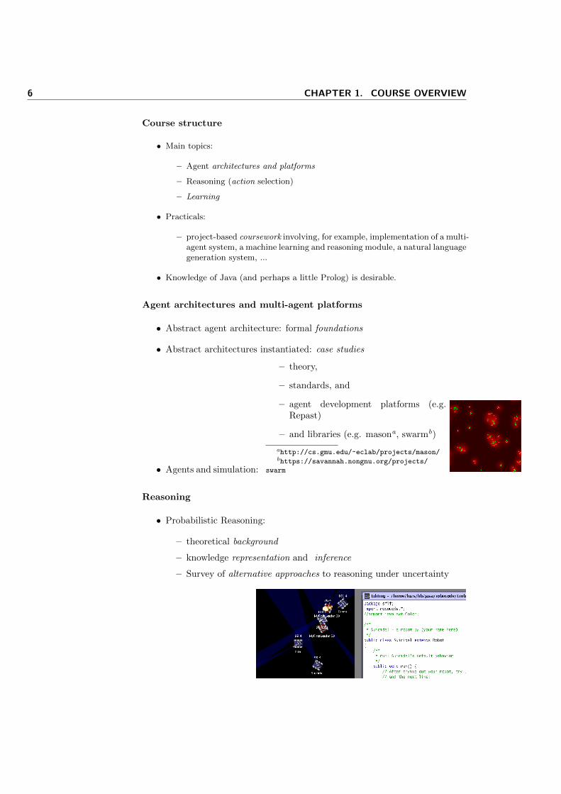
• Agents and simulation:
– theory,
– standards, and
– agent development platforms (e.g.Repast)
– and libraries (e.g. masona, swarmb)
ahttp://cs.gmu.edu/~eclab/projects/mason/bhttps://savannah.nongnu.org/projects/
swarm
Reasoning
• Probabilistic Reasoning:
– theoretical background
– knowledge representation and inference
– Survey of alternative approaches to reasoning under uncertainty
Chapter 1 7
Learning
• Machine learning: theoretical background
• Probabilistic learning: theory and applications
• Reinforcement learning
Coursework and Project
• Coursework-based assessment:
• Weekly labs and mini-assignments (30%)
• Longer project, to be delivered in January (70%):
– Entering an AI Game competition
– Reinforcement Learning for Off-The-Shelf games: use of a game simula-tor/server such as “Unreal Tournament 4” (UT2004) to create an agentthat learns.
– A Natural Language Generation system to enter the Give Challenge
– A project on communicating cooperative agents,
– ...
Multiagent systems course plan
• An overview: (Wooldridge, 2002) (Weiss, 1999, prologue):
– What are agents?
– What properties characterise them?
• Examples and issues
• Human vs. artificial agents
• Agents vs. objects
• Agents vs. expert systems
• Agents and User Interfaces
8 CHAPTER 1. COURSE OVERVIEW
A taxonomy of agent architectures
• Formal definition of an agent architecture (Weiss, 1999, chapter 1) and(Wooldridge, 2002)
• “Reactive” agents:
– Brooks’ subsumption architecture (Brooks, 1986)
– Artificial life
– Individual-based simulation
• “Reasoning” agents:
– Logic-based and BDI architectures
– Layered architectures
The term “reactive agents” is generally associated in the literature withthe work of Brooks and the use of the subsumption architecture in distributedproblem-solving. In this course, we will use the term to denote a larger classof agents not necessarily circumscribed to problem-solving. These include do-mains where one is primarily interested in observing, or systematically studyingpatterns emerging from interactions among many agents.
Reactive agents in detail
• Reactive agents in problem solving
• Individual-based simulation and modelling and computational modellingof complex phenomena:
– Discussion of different approaches
• Simulations as multi-agent interactions
• Case studies:
– Agent-based modelling of social interaction
– Agent-based modelling in biology
– Ant-colony optimisation
Logic-based agents (Not covered this year.)
• Coordination issues
• Communication protocols
• Reasoning
• Agent Communication Languages (ACL):
– KQML
– FIPA-ACL
• Ontology and semantics:
– KIF
– FIPA-SL
Chapter 1 9
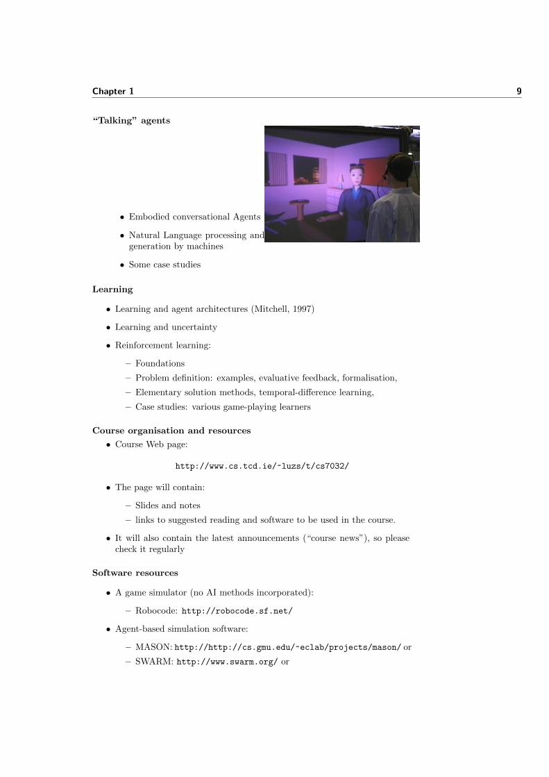
“Talking” agents
• Embodied conversational Agents
• Natural Language processing andgeneration by machines
• Some case studies
Learning
• Learning and agent architectures (Mitchell, 1997)
• Learning and uncertainty
• Reinforcement learning:
– Foundations
– Problem definition: examples, evaluative feedback, formalisation,
– Elementary solution methods, temporal-difference learning,
– Case studies: various game-playing learners
Course organisation and resources
• Course Web page:
http://www.cs.tcd.ie/~luzs/t/cs7032/
• The page will contain:
– Slides and notes
– links to suggested reading and software to be used in the course.
• It will also contain the latest announcements (“course news”), so pleasecheck it regularly
Software resources
• A game simulator (no AI methods incorporated):
– Robocode: http://robocode.sf.net/
• Agent-based simulation software:
– MASON: http://http://cs.gmu.edu/~eclab/projects/mason/ or
– SWARM: http://www.swarm.org/ or
10 CHAPTER 1. COURSE OVERVIEW
– REPAST http://repast.sourceforge.net/
• The Give Challenge website: http://www.give-challenge.org/research/
• See also:
– http://www.cs.tcd.ie/~luzs/t/cs7032/sw/
Reading for next week
• “Partial Formalizations and the Lemmings Game” (McCarthy, 1998).
– available on-line1;
– Prepare a short presentation (3 mins; work in groups of 2) for nextTuesday
Texts
• Useful references:
– Agents, probabilistic reasoning (Russell and Norvig, 2003)
– Agents, multiagent systems (Wooldridge, 2002)
– Reinforcement learning (Bertsekas and Tsitsiklis, 1996), (Sutton and Barto,1998)
• and also:
– (some) probabilistic reasoning, machine learning (Mitchell, 1997)
– Artificial Intelligence for Games (Millington, 2006)
– Research papers TBA...
1http://www.scss.tcd.ie/~luzs/t/cs7032/bib/McCarthyLemmings.pdf
2Agents: definition and formal architectures
Outline
• What is an agent?
• Properties one would like to model
• Mathematical notation
• A generic model
• A purely reactive model
• A state-transition model
• Modelling concrete architectures
• References: (Wooldridge, 2009, ch 1 and ch 2 up to section2.6), (Russelland Norvig, 2003, ch 2)
Abstract architectures will (hopefully) help us describe a taxonomy (as itwere) of agent-based systems, and the way designers and modellers of multi-agent systems see these artificial creatures. Although one might feel tempted tosee them as design tools, abstract architectures are really descriptive devices.Arguably their main purpose is to provide a framework in which a broad varietyof systems which one way or another have been identified as “agent systems”can be classified in terms of certain formal properties. In order to be able todescribe such a variety of systems, the abstract architecture has to be as generalas possible (i.e. it should not commit the modeller to a particular way of, say,describing how an agent chooses an action from its action repertoire). Onecould argue that such level of generality limits the usefulness of an abstractarchitecture to the creation of taxonomies. This might explain why this way oflooking at multi-agent systems hasn’t been widely adopted by agent developers.In any case, it has the merit of attempting to provide precise (if contentious)definitions of the main concepts involved thereby moving the discussion into amore formal domain.
12 CHAPTER 2. AGENTS: DEFINITION AND FORMAL ARCHITECTURES
What is an “agent”?
• “A person who acts on behalf of another” (Oxford American Dictionaries)
• Action, action delegation: state agents, travel agents, AgentSmith
• Action, simply (autonomy)
• “Artificial agents”: understanding machines by ascribing hu-man qualities to them (McCarthy, 1979) (humans do that allthe time)
• Interface agents: that irritating paper-clip
An example: Interface agents
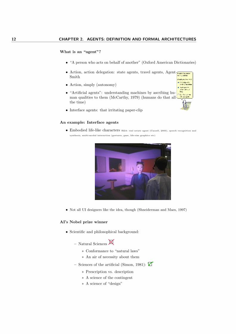
• Embodied life-like characters REA: real estate agent (Cassell, 2000), speech recognition and
synthesis, multi-modal interaction (gestures, gaze, life-size graphics etc)
• Not all UI designers like the idea, though (Shneiderman and Maes, 1997)
AI’s Nobel prize winner
• Scientific and philosophical background:
– Natural Sciences
∗ Conformance to “natural laws”
∗ An air of necessity about them
– Sciences of the artificial (Simon, 1981):
∗ Prescription vs. description
∗ A science of the contingent
∗ A science of “design”
Chapter 2 13
From a prescriptive (design) perspective...
• Agent properties:
– Autonomy: acting independently (of user/human intervention)
– Situatedness: sensing and modifying the environment
– Flexibility:
∗ re-activity to changes
∗ pro-activity in bringing about environmental conditions underwhich the agent’s goals can be achieved, and
∗ sociability: communicating with other agents, collaborating, andsometimes competing
In contrast with the notion of abstract architecture we develop below, theseproperties of multi-agent systems are useful from the point of view of conceptu-alising individual systems (or prompting the formation of a similar conceptualmodel by the user, in the case of interface agents). Abstract architectures, asdescriptive devices, will be mostly interested in the property of “situatedness”.The starting point is the assumption that an agent is essentially defined byits actions, and that an agent’s actions might be reactions to and bring aboutchanges in the environment. Obviously, there is more to agents and environ-ments than this. Agents typically exhibit goal-oriented behaviour, assess futureactions in terms of the measured performance of past actions, etc. The ar-chitectures described below will have little to say about these more complexnotions.
However, before presenting the abstract architecture, let’s take a look at ataxonomy that does try to place goals in context:
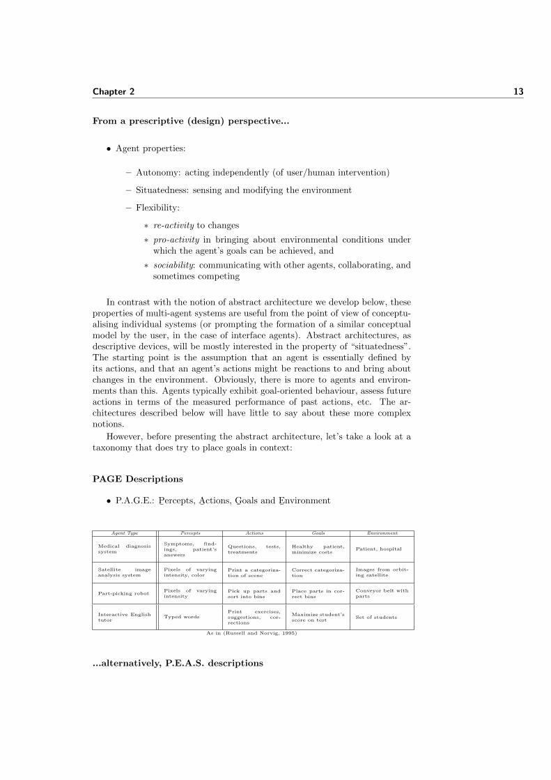
PAGE Descriptions
• P.A.G.E.: P¯
ercepts, A¯
ctions, G¯
oals and E¯
nvironment
Agent Type Percepts Actions Goals Environment
Medical diagnosissystem
Symptoms, find-ings, patient’sanswers
Questions, tests,treatments
Healthy patient,minimize costs
Patient, hospital
Satellite imageanalysis system
Pixels of varyingintensity, color
Print a categoriza-tion of scene
Correct categoriza-tion
Images from orbit-ing satellite
Part-picking robotPixels of varyingintensity
Pick up parts andsort into bins
Place parts in cor-rect bins
Conveyor belt withparts
Interactive Englishtutor
Typed wordsPrint exercises,suggestions, cor-rections
Maximize student’sscore on test
Set of students
As in (Russell and Norvig, 1995)
...alternatively, P.E.A.S. descriptions
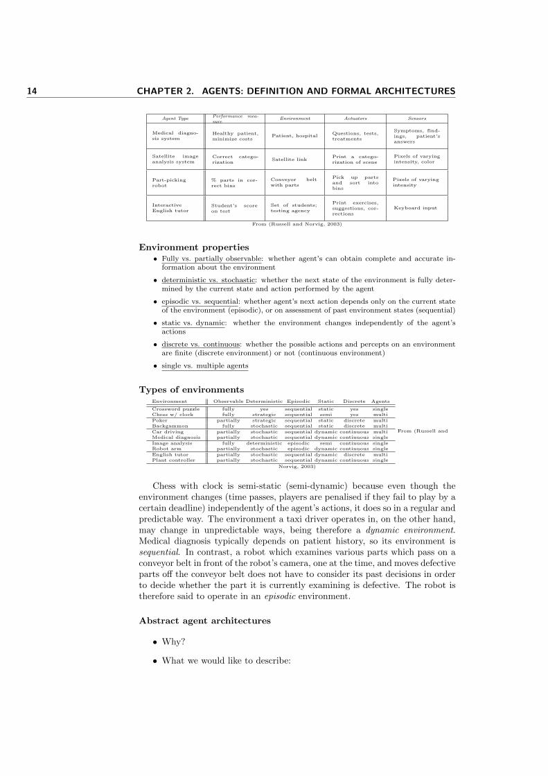
14 CHAPTER 2. AGENTS: DEFINITION AND FORMAL ARCHITECTURES
Agent TypePerformance mea-sure
Environment Actuators Sensors
Medical diagno-sis system
Healthy patient,minimize costs
Patient, hospitalQuestions, tests,treatments
Symptoms, find-ings, patient’sanswers
Satellite imageanalysis system
Correct catego-rization
Satellite linkPrint a catego-rization of scene
Pixels of varyingintensity, color
Part-pickingrobot
% parts in cor-rect bins
Conveyor beltwith parts
Pick up partsand sort intobins
Pixels of varyingintensity
InteractiveEnglish tutor
Student’s scoreon test
Set of students;testing agency
Print exercises,suggestions, cor-rections
Keyboard input
From (Russell and Norvig, 2003)
Environment properties• Fully vs. partially observable: whether agent’s can obtain complete and accurate in-
formation about the environment
• deterministic vs. stochastic: whether the next state of the environment is fully deter-mined by the current state and action performed by the agent
• episodic vs. sequential: whether agent’s next action depends only on the current stateof the environment (episodic), or on assessment of past environment states (sequential)
• static vs. dynamic: whether the environment changes independently of the agent’sactions
• discrete vs. continuous: whether the possible actions and percepts on an environmentare finite (discrete environment) or not (continuous environment)
• single vs. multiple agents
Types of environmentsEnvironment Observable Deterministic Episodic Static Discrete Agents
Crossword puzzle fully yes sequential static yes singleChess w/ clock fully strategic sequential semi yes multi
Poker partially strategic sequential static discrete multiBackgammon fully stochastic sequential static discrete multi
Car driving partially stochastic sequential dynamic continuous multiMedical diagnosis partially stochastic sequential dynamic continuous single
Image analysis fully deterministic episodic semi continuous singleRobot arm partially stochastic episodic dynamic continuous single
English tutor partially stochastic sequential dynamic discrete multiPlant controller partially stochastic sequential dynamic continuous single
From (Russell and
Norvig, 2003)
Chess with clock is semi-static (semi-dynamic) because even though theenvironment changes (time passes, players are penalised if they fail to play by acertain deadline) independently of the agent’s actions, it does so in a regular andpredictable way. The environment a taxi driver operates in, on the other hand,may change in unpredictable ways, being therefore a dynamic environment.Medical diagnosis typically depends on patient history, so its environment issequential. In contrast, a robot which examines various parts which pass on aconveyor belt in front of the robot’s camera, one at the time, and moves defectiveparts off the conveyor belt does not have to consider its past decisions in orderto decide whether the part it is currently examining is defective. The robot istherefore said to operate in an episodic environment.
Abstract agent architectures
• Why?
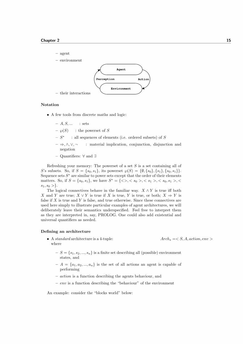
• What we would like to describe:
Chapter 2 15
– agent
– environment
– their interactionsEnvironment
Agent
Perception Action
Notation
• A few tools from discrete maths and logic:
– A,S, ... : sets
– ℘(S) : the powerset of S
– S∗ : all sequences of elements (i.e. ordered subsets) of S
– ⇒,∧,∨,¬ : material implication, conjunction, disjunction andnegation
– Quantifiers: ∀ and ∃
Refreshing your memory: The powerset of a set S is a set containing all ofS’s subsets. So, if S = {s0, s1}, its powerset ℘(S) = {∅, {s0}, {s1}, {s0, s1}}.Sequence sets S∗ are similar to power sets except that the order of their elementsmatters. So, if S = {s0, s1}, we have S∗ = {<>,< s0 >,< s1 >,< s0, s1 >,<s1, s0 >}.
The logical connectives behave in the familiar way. X ∧ Y is true iff bothX and Y are true; X ∨ Y is true if X is true, Y is true, or both; X ⇒ Y isfalse if X is true and Y is false, and true otherwise. Since these connectives areused here simply to illustrate particular examples of agent architectures, we willdeliberately leave their semantics underspecified. Feel free to interpret themas they are interpreted in, say, PROLOG. One could also add existential anduniversal quantifiers as needed.
Defining an architecture
• A standard architecture is a 4-tuple: Archs =< S,A, action, env >where
– S = {s1, s2, ..., sn} is a finite set describing all (possible) environmentstates, and
– A = {a1, a2, ..., an} is the set of all actions an agent is capable ofperforming
– action is a function describing the agents behaviour, and
– env is a function describing the “behaviour” of the environment
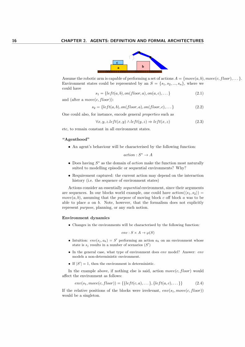
An example: consider the “blocks world” below:
16 CHAPTER 2. AGENTS: DEFINITION AND FORMAL ARCHITECTURES
������������������������������������������������������������������������������������������������������������������������������������������������
a
c
b
Assume the robotic arm is capable of performing a set of actionsA = {move(a, b),move(c, floor), . . . }.Environment states could be represented by an S = {s1, s2, ..., sn}, where wecould have
s1 = {left(a, b), on(floor, a), on(a, c), . . . } (2.1)
and (after a move(c, floor)):
s2 = {left(a, b), on(floor, a), on(floor, c), . . . } (2.2)
One could also, for instance, encode general properties such as
∀x, y, z.left(x, y) ∧ left(y, z)⇒ left(x, z) (2.3)
etc, to remain constant in all environment states.
“Agenthood”
• An agent’s behaviour will be characterised by the following function:
action : S∗ → A
• Does having S∗ as the domain of action make the function most naturallysuited to modelling episodic or sequential environments? Why?
• Requirement captured: the current action may depend on the interactionhistory (i.e. the sequence of environment states)
Actions consider an essentially sequential environment, since their argumentsare sequences. In our blocks world example, one could have action(〈s1, s2〉) =move(a, b), assuming that the purpose of moving block c off block a was to beable to place a on b. Note, however, that the formalism does not explicitlyrepresent purpose, planning, or any such notion.
Environment dynamics
• Changes in the environments will be characterised by the following function:
env : S ×A→ ℘(S)
• Intuition: env(sj , ak) = S′ performing an action ak on an environment whosestate is sj results in a number of scenarios (S′)
• In the general case, what type of environment does env model? Answer: envmodels a non-deterministic environment.
• If |S′| = 1, then the environment is deterministic.
In the example above, if nothing else is said, action move(c, floor) wouldaffect the environment as follows:
env(s1,move(c, floor)) = {{left(c, a), . . . }, {left(a, c), . . . }} (2.4)
If the relative positions of the blocks were irrelevant, env(s1,move(c, floor))would be a singleton.
Chapter 2 17
Interaction history
• The agent-environment interaction will be characterized as follows:
h : s0a0→ s1
a1→ ...au−1→ su
au→ ...
• h is a possible history of the agent in the environment iff :
∀u ∈ N, au = action(< s0, ..., su >) (2.5)
and∀u > 0 ∈ N, su ∈ env(su−1, au−1) (2.6)
Condition (2.5) guarantees that all actions in a history apply to environmentstates in that history.
Condition (2.6) guarantees that all environment states in a history (exceptthe initial state) “result” from actions performed on environment states.
Characteristic behaviour
• Characteristic behaviour is defined as a set of interaction histories
hist = {h0, h1, ..., hn}
where
• each hi is a possible history for the agent in the environment
Invariant properties
• We say that φ is an invariant property of an agent architecture iff
For all histories h ∈ hist and states s ∈ S φis a property of s (written s |= φ)
• We will leave the relation |= underspecified for the time being.
– In architectures where agents have minimal symbolic reasoning abili-ties (e.g. some concrete reactive architectures), |= could be translatedsimply as set membership, that is s |= φ ⇔ φ ∈ s, in architectureswhere reasoning isn’t performed
Behavioural equivalence
• Equivalence of behaviours is defined as follows (in an abstract architecture)
An agent ag1 is regarded as equivalent toagent ag2 with respect to environment enviiff hist(ag1, envi) = hist(ag2, envi)
• When the condition above holds for all environments envi, then we simplysay that ag1 and ag2 have equivalent behaviour
18 CHAPTER 2. AGENTS: DEFINITION AND FORMAL ARCHITECTURES
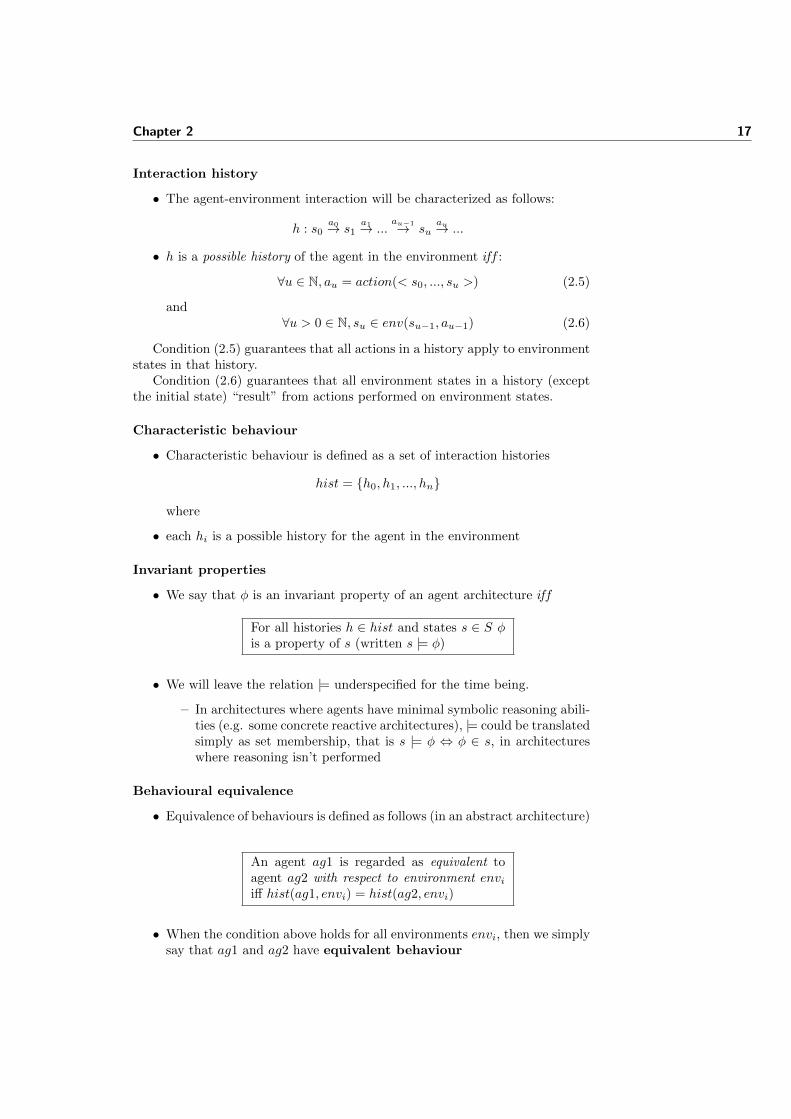
Modelling reactive agents
• Reactive architectures
– production rules
– a scheme for defining priorities in the application of rules (e.g. sub-sumption (Brooks, 1986))
Perception
Action
Explore
Move forward
Avoid Obstacles
Wander
...
– no reasoning (theorem proving or planning) involved
Abstract reactive agents
• Purely reactive agents can be modelled by assuming
action : S → A
• Everything else remains as in the general (standard abstract architecture)case:
Archr =< S,A, actionr, env >
• Abstract reactive agents operate essentially on an episodic view of envi-ronments (i.e. they are memoryless agents). See slide 16
Example: a thermostat.temperature(cold)⇒ do(heater(on))¬temperature(cold)⇒ do(heater(off))S = {{temperature(cold)}, {¬temperature(cold)}}A = {heater(on), heater(off)}
Purely reactive vs. standard agents
• Proposition 1 (exercise):
Purely reactive agents form a proper subclass of standardagents. That is, for any given environment description S,and action repertoire A:
(i) every purely reactive agent is behaviourally equiva-lent to a standard agent, and
(ii) the reverse does not hold.
Chapter 2 19
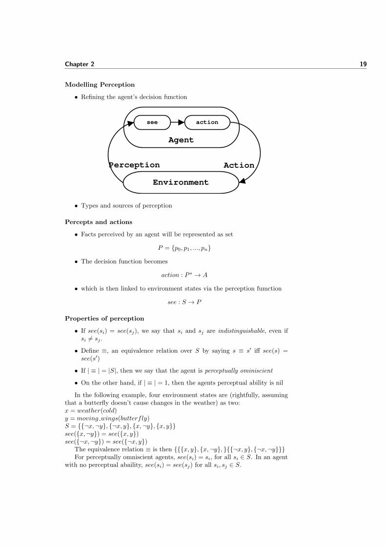
Modelling Perception
• Refining the agent’s decision function
Environment
Agent
Perception Action
see action
• Types and sources of perception
Percepts and actions
• Facts perceived by an agent will be represented as set
P = {p0, p1, ..., pn}
• The decision function becomes
action : P ∗ → A
• which is then linked to environment states via the perception fumction
see : S → P
Properties of perception
• If see(si) = see(sj), we say that si and sj are indistinguishable, even ifsi 6= sj .
• Define ≡, an equivalence relation over S by saying s ≡ s′ iff see(s) =see(s′)
• If | ≡ | = |S|, then we say that the agent is perceptually ominiscient
• On the other hand, if | ≡ | = 1, then the agents perceptual ability is nil
In the following example, four environment states are (rightfully, assumingthat a butterfly doesn’t cause changes in the weather) as two:x = weather(cold)y = moving wings(butterfly)S = {{¬x,¬y}, {¬x, y}, {x,¬y}, {x, y}}see({x,¬y}) = see({x, y})see({¬x,¬y}) = see({¬x, y})
The equivalence relation ≡ is then {{{x, y}, {x,¬y}, }{{¬x, y}, {¬x,¬y}}}For perceptually omniscient agents, see(si) = si, for all si ∈ S. In an agent
with no perceptual abaility, see(si) = see(sj) for all si, sj ∈ S.
20 CHAPTER 2. AGENTS: DEFINITION AND FORMAL ARCHITECTURES
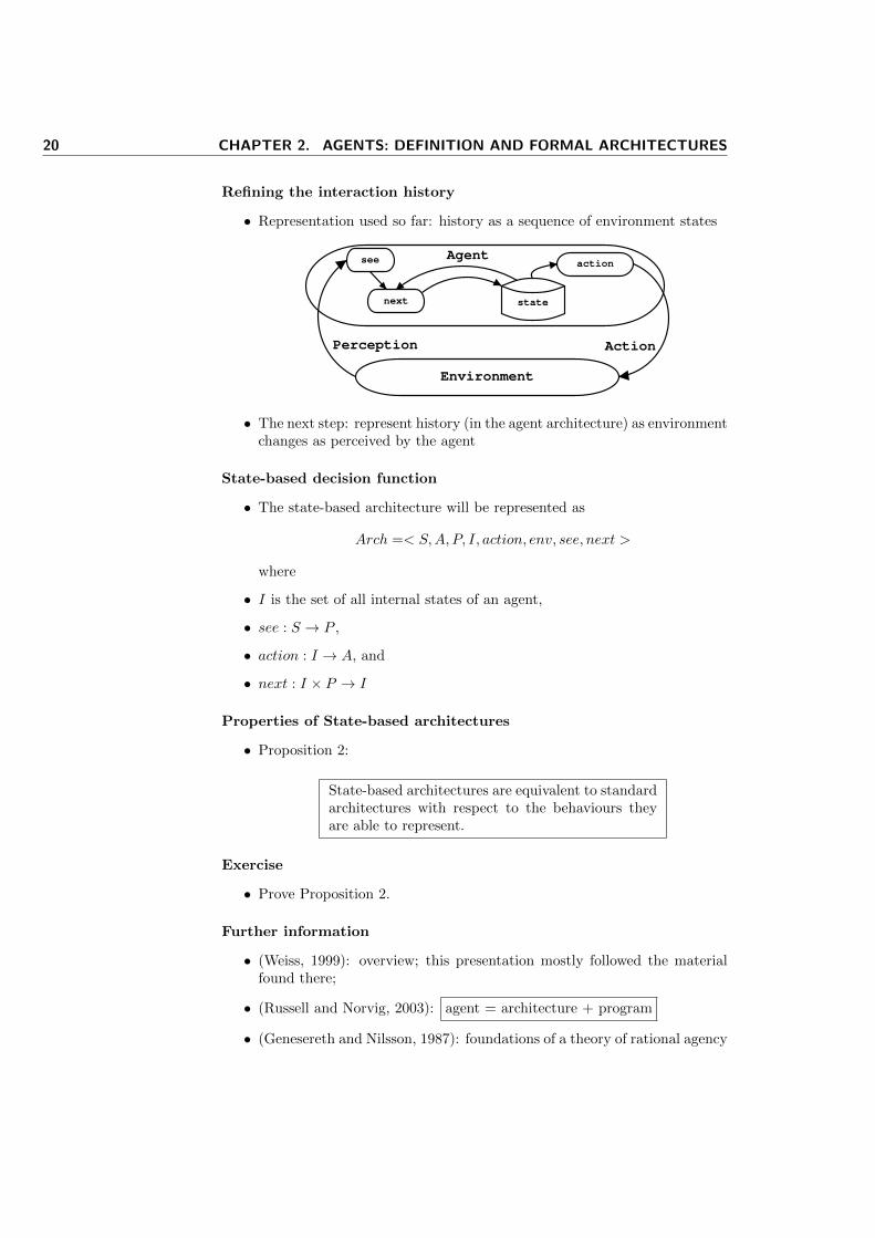
Refining the interaction history
• Representation used so far: history as a sequence of environment states
Environment
Perception Action
see action
next state
Agent
• The next step: represent history (in the agent architecture) as environmentchanges as perceived by the agent
State-based decision function
• The state-based architecture will be represented as
Arch =< S,A, P, I, action, env, see, next >
where
• I is the set of all internal states of an agent,
• see : S → P ,
• action : I → A, and
• next : I × P → I
Properties of State-based architectures
• Proposition 2:
State-based architectures are equivalent to standardarchitectures with respect to the behaviours theyare able to represent.
Exercise
• Prove Proposition 2.
Further information
• (Weiss, 1999): overview; this presentation mostly followed the materialfound there;
• (Russell and Norvig, 2003): agent = architecture + program
• (Genesereth and Nilsson, 1987): foundations of a theory of rational agency
3Practical: Creating a simple robocode agent
3.1 Goals
In this exercise we will aim at (1) understanding how the Robocode1 simulatorworks, (2) to building a simple “robot”, and (3) describing it in terms an theabstract agent architecture introduced in the last lecture2.
In this lab we use Robocode version 1.0.7 which can be downloaded fromsourceforge3. Alternatively, if you prefer experimenting with PROLOG, youcan specify robots declaratively using a modified (and not very well tested, I’mafraid) version of the simulator.
3.2 Robocode: Getting started
The Robocode simulator should be installed in the IET Lab.
• http://robocode.sf.net/
In order to run the simulator, change directory to ROBOCODE_HOME and runrobocode.sh (on Unix) or robocode.bat (on Windows). This will bring up awindow displaying the “battlefield” (Fig. 3.1). Once the battlefield is visible,you may start a new battle by selecting Battle->New. You can create your firstrobot by starting the editor Robot->Editor and File->New->Robot. Inspectthe robot template (that’s already a fully functional, if not very clever, robot).Create a sub-directory of robots named by your initials (in lowercase) so thatyour robots will have a unique identifier, and select it as your code repositorythrough File->Save as..., ignoring Robocode’s suggestions.
Now, start a new battle and put your newly created robot to fight againstsome of the robots included in the Robocode distribution.
1http://robocode.sf.net/2http://www.cs.tcd.ie/~luzs/t/cs7032/abstractarch-notes.pdf3http://robocode.sf.net/
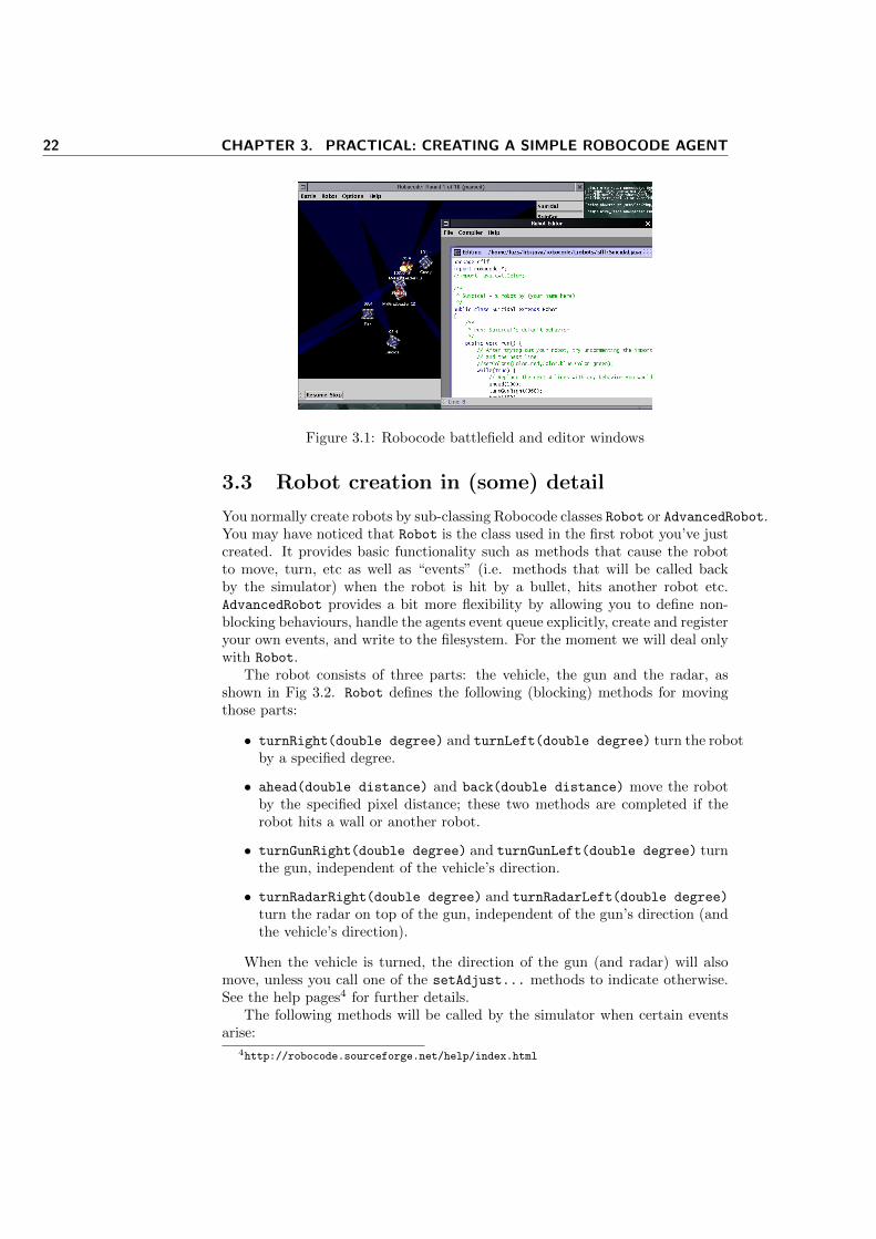
22 CHAPTER 3. PRACTICAL: CREATING A SIMPLE ROBOCODE AGENT
Figure 3.1: Robocode battlefield and editor windows
3.3 Robot creation in (some) detail
You normally create robots by sub-classing Robocode classes Robot or AdvancedRobot.You may have noticed that Robot is the class used in the first robot you’ve justcreated. It provides basic functionality such as methods that cause the robotto move, turn, etc as well as “events” (i.e. methods that will be called backby the simulator) when the robot is hit by a bullet, hits another robot etc.AdvancedRobot provides a bit more flexibility by allowing you to define non-blocking behaviours, handle the agents event queue explicitly, create and registeryour own events, and write to the filesystem. For the moment we will deal onlywith Robot.
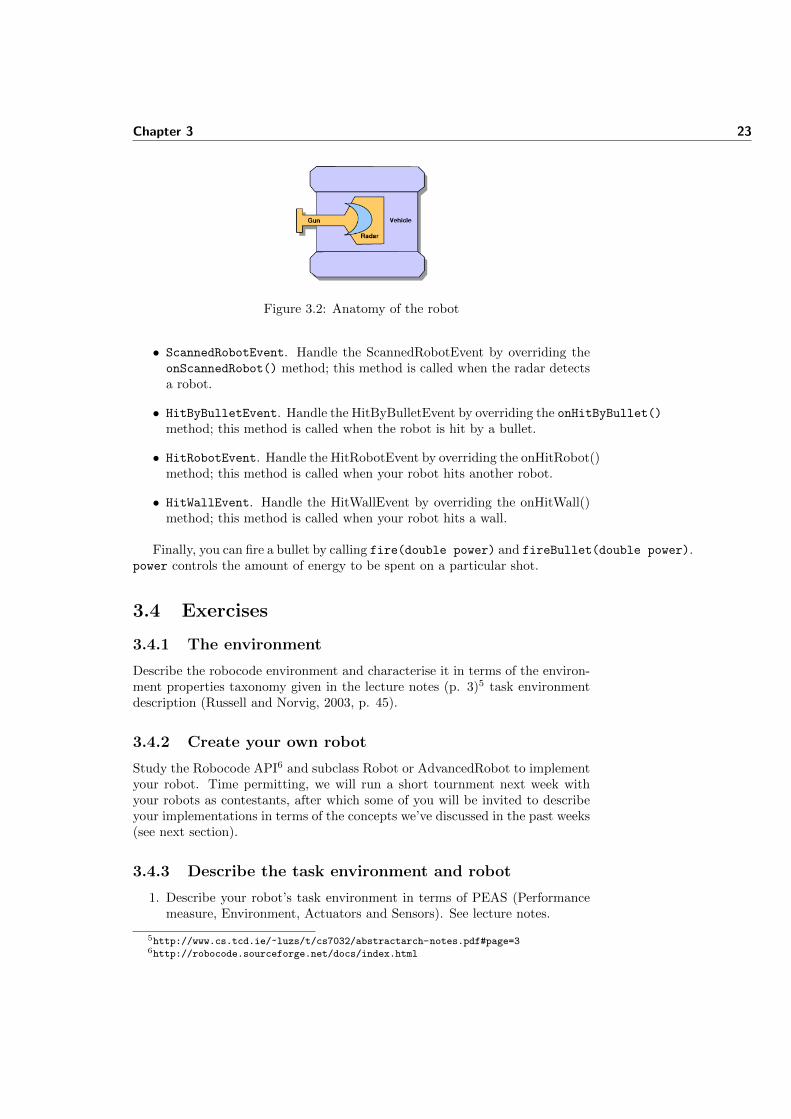
The robot consists of three parts: the vehicle, the gun and the radar, asshown in Fig 3.2. Robot defines the following (blocking) methods for movingthose parts:
• turnRight(double degree) and turnLeft(double degree) turn the robotby a specified degree.
• ahead(double distance) and back(double distance) move the robotby the specified pixel distance; these two methods are completed if therobot hits a wall or another robot.
• turnGunRight(double degree) and turnGunLeft(double degree) turnthe gun, independent of the vehicle’s direction.
• turnRadarRight(double degree) and turnRadarLeft(double degree)
turn the radar on top of the gun, independent of the gun’s direction (andthe vehicle’s direction).
When the vehicle is turned, the direction of the gun (and radar) will alsomove, unless you call one of the setAdjust... methods to indicate otherwise.See the help pages4 for further details.
The following methods will be called by the simulator when certain eventsarise:
4http://robocode.sourceforge.net/help/index.html
Chapter 3 23
Figure 3.2: Anatomy of the robot
• ScannedRobotEvent. Handle the ScannedRobotEvent by overriding theonScannedRobot() method; this method is called when the radar detectsa robot.
• HitByBulletEvent. Handle the HitByBulletEvent by overriding the onHitByBullet()method; this method is called when the robot is hit by a bullet.
• HitRobotEvent. Handle the HitRobotEvent by overriding the onHitRobot()method; this method is called when your robot hits another robot.
• HitWallEvent. Handle the HitWallEvent by overriding the onHitWall()method; this method is called when your robot hits a wall.
Finally, you can fire a bullet by calling fire(double power) and fireBullet(double power).power controls the amount of energy to be spent on a particular shot.
3.4 Exercises
3.4.1 The environment
Describe the robocode environment and characterise it in terms of the environ-ment properties taxonomy given in the lecture notes (p. 3)5 task environmentdescription (Russell and Norvig, 2003, p. 45).
3.4.2 Create your own robot
Study the Robocode API6 and subclass Robot or AdvancedRobot to implementyour robot. Time permitting, we will run a short tournment next week withyour robots as contestants, after which some of you will be invited to describeyour implementations in terms of the concepts we’ve discussed in the past weeks(see next section).
3.4.3 Describe the task environment and robot
1. Describe your robot’s task environment in terms of PEAS (Performancemeasure, Environment, Actuators and Sensors). See lecture notes.
5http://www.cs.tcd.ie/~luzs/t/cs7032/abstractarch-notes.pdf#page=36http://robocode.sourceforge.net/docs/index.html
24 CHAPTER 3. PRACTICAL: CREATING A SIMPLE ROBOCODE AGENT
2. Describe your robot and the enrironment it operates in as a logic-based(aka knowledge-based) agent architecture.
Specifically, you should describe the environment S, the events the agentis capable of perceiving, the actions (A) it is capable of performing, theenvironmental configurations that trigger certain actions and the environ-mental changes (if any) that they bring about. Facts, states and actionsmay be described with PROLOG clauses or predicate logic expressions,for instance.
What sort of abstract architecture would most adequately describe yourrobot? Why? What are the main difficulties in describing robots thisway?
3.4.4 PROLOG Robots (optional)
In the course’s software repository7 you will find a (gzip’d) tarball contain-ing the source code of an earlier version of the robocode simulator (1.0.7,the first open-source release) which I have modified so that it allows you towrite your robocode declaratively, in Prolog. The main modifications are inrobocode/robolog/*.java, which include a new class manager and loaderadapted to deal with Prolog code (identified by extension .pro). The classmanager (RobologClassManager) assigns each Prolog robot a LogicalPeer
which does the interface between the simulator and Prolog “theories”. SomeProlog code ( robocode/robolog/*.pro) handle the other end of the inter-face: actioninterface.pro contains predicates which invoke action methodson Robot objects, and environinterface.pro predicates that retrieve infor-mation from the battlefield. All these predicates will be available to yourrobots. A simple logical robot illustrating how this works can be found inbindist/robots/log/LogBot.pro.
The archive contains a Makefile which you can use to compile the codeand generate a ‘binary’ distribution analogous to the pre-installed robocodeenvironment (make bindist). Alternatively, you can download a pre-compiledversion8 from the course website.
Build a Prolog robot. Do you think there are advantages in being able tospecify your robot’s behaviour declaratively? If so, perhaps you could consideradapting ‘robolog’ to the latest version of robocode and contributing the codeto the project.
7http://www.cs.tcd.ie/~luzs/t/cs7032/sw/robolog-0.0.1-1.0.7.tar.gz8http://www.cs.tcd.ie/~luzs/t/cs7032/sw/robolog-0.0.1-1.0.7-bin.tar.gz
4Utility functions and Concrete architectures:
deductive agents
Abstract Architectures (ctd.)
• An agent’s behaviour is encoded as its history:
h : s0a0→ s1
a1→ ...au−1→ su
au→ ...
• Define:
– HA: set of all histories which end with an action
– HS : histories which end in environment states
• A state transformer function τ : HA → ℘(S) represents the effect an agenthas on an environment.
• So we may represent environment dynamics by a triple:
Env =< S, s0, τ >
• And similarly, agent dynamics as
Ag : HS → A
The architecture described in this slide and in (Wooldridge, 2002) appearsto be an attempt to address some limitations of the formalisation described inthe Abstract Architecture Notes. In that model, action and env — describingrespectively the agent’s choice of action given an environment, and possiblechanges in the environment given an action — are regarded as “primitives”(in the sense that these are the basic concepts of which the other concepts inthe architecture are derived). As the framework strives to be general enough todescribe a large variety of agent systems, no assumptions are made about causalconnections between actions and changes in the environment. Furthermore,although the history of environmental changes is assumed to be available to theagent as it chooses an action (recall the function’s signature action : S∗ → A),no specific structure exists which encodes action history.
26CHAPTER 4. UTILITY FUNCTIONS AND CONCRETE ARCHITECTURES: DEDUCTIVE
AGENTS
The new model proposed here builds on efforts originating in AI (Geneserethand Nilsson, 1987, ch 14) and theoretical computer science (Fagin et al., 1995,p 154) and apparently attempts to provide an account of both action and envi-ronment history. The primitive used for describing an agent’s behaviour is nolonger an action fuction, as defined above, but a history (or run, as in (Faginet al., 1995)):
h : s0a0→ s1
a1→ ...au−1→ su
au→ ...
If one defines:
• HA: the set of all histories which end with an action
• HS : the histories which end in environment states
Then a state transformer function τ : HA → ℘(S) represents the way the envi-ronment changes as actions are performed. (Or would it be the effect an agenthas on its environment? Note that the issue of causality is never satisfactorilyaddressed), and the “environment dynamics” can be described as a triple:
Env =< S, s0, τ > (4.1)
and the action function redefined as action : HS → A.Although this approach seems more adequate, (Wooldridge, 2002) soon
abandons it in favour of a variant the first one when perception is incorporatedto the framework (i.e. the action function becomes action : P ∗ → A).
Utility functions
• Problem: how to “tell agents what to do”? (when exhaustive specificationis impractical)
• Decision theory (see (Russell and Norvig, 1995, ch. 16)):
– associate utilities (a performance measure) to states:
u : S → R
– Or, better yet, to histories:
u : H → R
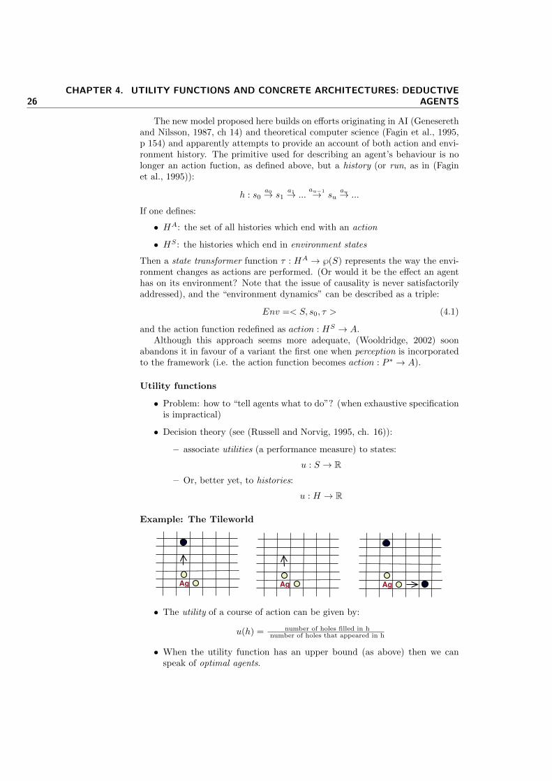
Example: The Tileworld
Ag Ag Ag
• The utility of a course of action can be given by:
u(h) = number of holes filled in hnumber of holes that appeared in h
• When the utility function has an upper bound (as above) then we canspeak of optimal agents.
Chapter 4 27
Optimal agents
• Let P (h|Ag,Env) denote the probability that h occurs when agent Ag isplaced in Env.
• Clearly ∑h∈H
P (h|Ag,Env) = 1 (4.2)
• An optimal agent Agopt in an environment Env will maximise expectedutility:
Agopt = arg maxAg
∑h∈H
u(h)P (h|Ag,Env) (4.3)
From abstract to concrete architectures
• Moving from abstract to concrete architectures is a matter of further spec-ifying action (e.g. by means of algorithmic description) and choosing anunderlying form of representation.
• Different ways of specifying the action function and representing knowl-edge:
– Logic-based: decision function implemented as a theorem prover(plus control layer)
– Reactive: (hierarchical) condition → action rules
– BDI: manipulation of data structures representing Beliefs, Desiresand Intentions
– Layered: combination of logic-based (or BDI) and reactive decisionstrategies
Logic-based architectures
• AKA Deductive Architectures
• Background: symbolic AI
– Knowledge representation by means of logical formulae
– “Syntactic” symbol manipulation
– Specification in logic ⇒ executable specification
• “Ingredients”:
– Internal states: sets of (say, first-order logic) formulae
∗ ∆ = {temp(roomA, 20), heater(on), ...}– Environment state and perception,
– Internal state seen as a set of beliefs
– Closure under logical implication (⇒):
∗ closure(∆,⇒) = {ϕ|ϕ ∈ ∆ ∨ ∃ψ.ψ ∈ ∆ ∧ ψ ⇒ ϕ}– (is this a reasonable model of an agent’s beliefs?)
28CHAPTER 4. UTILITY FUNCTIONS AND CONCRETE ARCHITECTURES: DEDUCTIVE
AGENTS
About whether logical closure (say, first-order logic) corresponds to a rea-sonable model of an agent’s beliefs, the answer is likely no (at if we are talkingabout human-like agents). One could, for instance, know all of axioms Peano’saxioms1 for natural numbers and still not know whether Goldbach’s conjecture2
(that all even numbers greater than 2 is the sum of two primes).
Representing deductive agents
• We will use the following objects:
– L: a set of sentences of a logical system
∗ As defined, for instance, by the usual wellformedness rules forfirst-order logic
– D = ℘(L): the set of databases of L
– ∆0, ...,∆n ∈ D: the agent’s internal states (or beliefs)
– |=ρ: a deduction relation described by the deduction rules ρ chosenfor L: We write ∆ |=ρ ϕ if ϕ ∈ closure(∆, ρ)
Describing the architecture
• A logic-based architecture is described by the following structure:
ArchL =< L,A, P,D, action, env, see, next > (4.4)
• The update function consists of additions and removals of facts from thecurrent database of internal states:
– next : D × P → D
∗ old: removal of “old” facts
∗ new: addition of new facts (brought about by action)
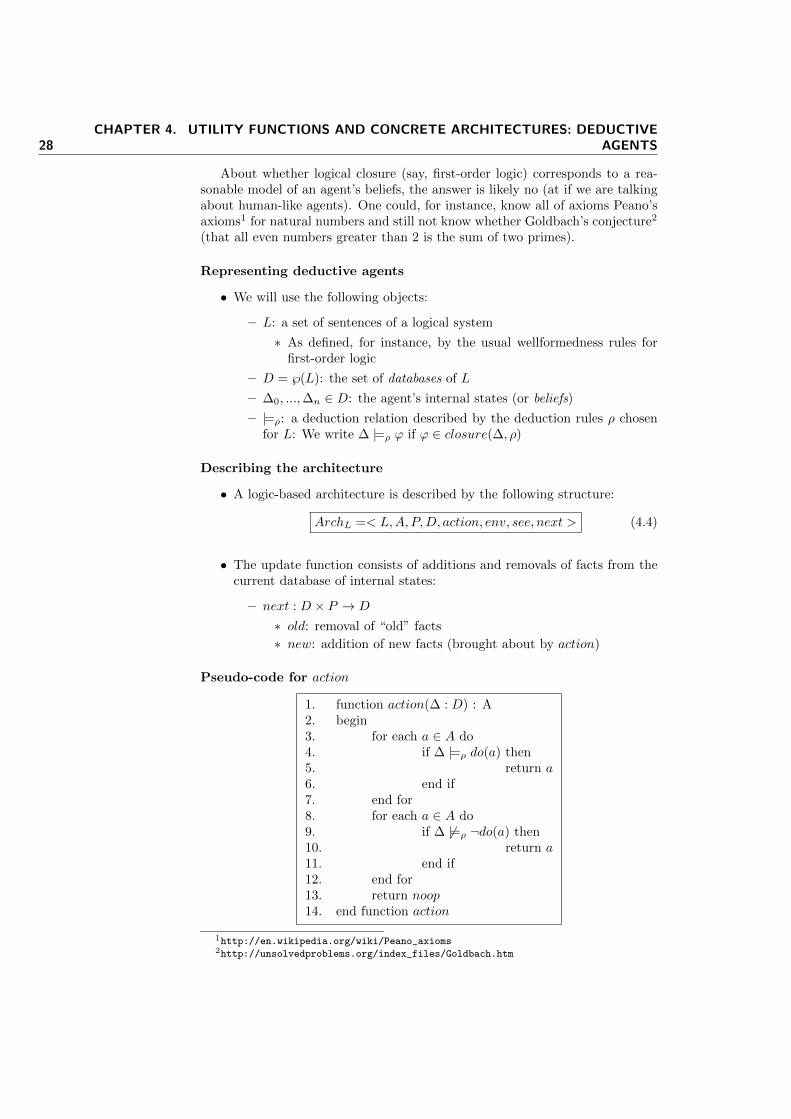
Pseudo-code for action
1. function action(∆ : D) : A2. begin3. for each a ∈ A do4. if ∆ |=ρ do(a) then5. return a6. end if7. end for8. for each a ∈ A do9. if ∆ 6|=ρ ¬do(a) then10. return a11. end if12. end for13. return noop14. end function action
1http://en.wikipedia.org/wiki/Peano_axioms2http://unsolvedproblems.org/index_files/Goldbach.htm
Chapter 4 29
Environment and Belief states
• The environment change function, env, remains as before.
• The belief database update function could be further specified as follows
next(∆, p) = (∆ \ old(∆)) ∪ new(∆, p) (4.5)
where old(∆) represent beliefs no longer held (as a consequence of action),and new(∆, p) new beliefs that follow from facts perceived about the newenvironmental conditions.
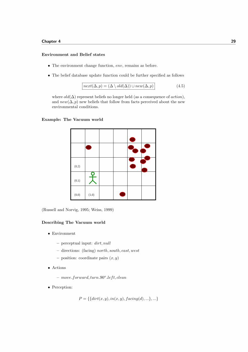
Example: The Vacuum world
(1,0)(0,0)
(0,1)
(0,2)
(Russell and Norvig, 1995; Weiss, 1999)
Describing The Vacuum world
• Environment
– perceptual input: dirt, null
– directions: (facing) north, south, east, west
– position: coordinate pairs (x, y)
• Actions
– move forward, turn 90o left, clean
• Perception:
P = {{dirt(x, y), in(x, y), facing(d), ...}, ...}
30CHAPTER 4. UTILITY FUNCTIONS AND CONCRETE ARCHITECTURES: DEDUCTIVE
AGENTS
Deduction rules
• Part of the decision function
• Format (for this example):
– P (...)⇒ Q(...)
• PROLOG fans may think of these rules as Horn Clauses.
• Examples:
– in(x, y) ∧ dirt(x, y)⇒ do(clean)
– in(x, 2) ∧ ¬dirt(x, y) ∧ facing(north)⇒ do(turn)
– in(0, 0) ∧ ¬dirt(x, y) ∧ facing(north)⇒ do(forward)
– ...
Updating the internal state database
• next(∆, p) = (∆ \ old(∆)) ∪ new(∆, p)
• old(∆) = {(P (t1, ..., tn)|P ∈ {in, dirt, facing} ∧ P (t1, ..., tn) ∈ ∆}
• new(∆, p) :
– update agent’s position,
– update agent’s orientation,
– etc
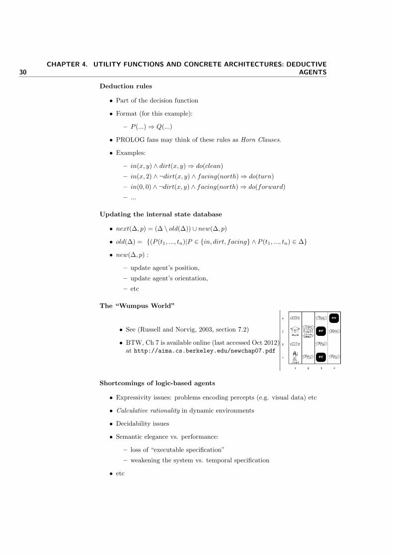
The “Wumpus World”
• See (Russell and Norvig, 2003, section 7.2)
• BTW, Ch 7 is available online (last accessed Oct 2012)at http://aima.cs.berkeley.edu/newchap07.pdf
Shortcomings of logic-based agents
• Expressivity issues: problems encoding percepts (e.g. visual data) etc
• Calculative rationality in dynamic environments
• Decidability issues
• Semantic elegance vs. performance:
– loss of “executable specification”
– weakening the system vs. temporal specification
• etc
Chapter 4 31
Existing (??) logic-based systems
• MetameM, Concurrent MetameM: specifications in temporal logic, model-checking as inference engine (Fisher, 1994)
• CONGOLOG: Situation calculus
• Situated automata: compiled logical specifications (Kaelbling and Rosen-schein, 1990)
• AgentSpeak, ...
• (see (Weiss, 1999) or (Wooldridge, 2002) for more details)
BDI Agents
• Implement a combination of:
– deductive reasoning (deliberation) and
– planning (means-ends reasoning)
Planning
• Planning formalisms describe actions in terms of (sets of) preconditions(Pa), delete lists (Da) and add lists (Aa):
< Pa, Da, Aa >
• E.g. Action encoded in STRIPS (for the “block’s world” example):
Stack(x,y):pre: clear(y), holding(x)del: clear(y), holding(x)add: armEmpty, on(x,y)
Planning problems
• A planning problem < ∆, O, γ > is determined by:
– the agent’s beliefs about the initial environment (a set ∆)
– a set of operator descriptors corresponding to the actions availableto the agent:
O = {< Pa, Da, Aa > |a ∈ A}– a set of formulae representing the goal/intention to be achieved (say,γ)
• A plan π =< ai, ..., an > determines a sequence ∆0, ...,∆n+1 where ∆0 =∆ and ∆i = (∆i−1 \Dai) ∪Aai , for 1 ≤ i ≤ n.

32CHAPTER 4. UTILITY FUNCTIONS AND CONCRETE ARCHITECTURES: DEDUCTIVE
AGENTS
Suggestions
• Investigate the use of BDI systems and agents in games.
• See, for instance, (Norling and Sonenberg, 2004) which describe the im-plementation of interactive BDI characters for Quake 2.
• And (Wooldridge, 2002, ch. 4), for some background.
• There are a number of BDI-based agent platforms around. ‘Jason’, forinstance, seems interesting:
http://jason.sourceforge.net/
5Reactive agents & Simulation
Concrete vs. abstract architectures
• Different ways of specifying the action
– Logic-based: decision function implemented as a theorem prover(plus control layer)
– Reactive: (hierarchical) condition → action rules
– BDI: manipulation of data structures representing Beliefs, Desiresand Intentions
– Layered: combination of logic-based (or BDI) and reactive decisionstrategies
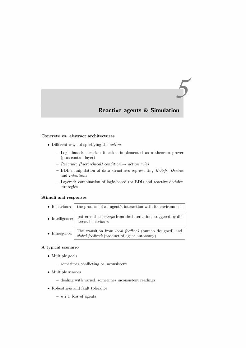
Stimuli and responses
• Behaviour: the product of an agent’s interaction with its environment
• Intelligence:patterns that emerge from the interactions triggered by dif-ferent behaviours
• Emergence:The transition from local feedback (human designed) andglobal feedback (product of agent autonomy).
A typical scenario
• Multiple goals
– sometimes conflicting or inconsistent
• Multiple sensors
– dealing with varied, sometimes inconsistent readings
• Robustness and fault tolerance
– w.r.t. loss of agents
34 CHAPTER 5. REACTIVE AGENTS & SIMULATION
• Additivity
– the more sensors and capabilities, the more processing power theagent needs
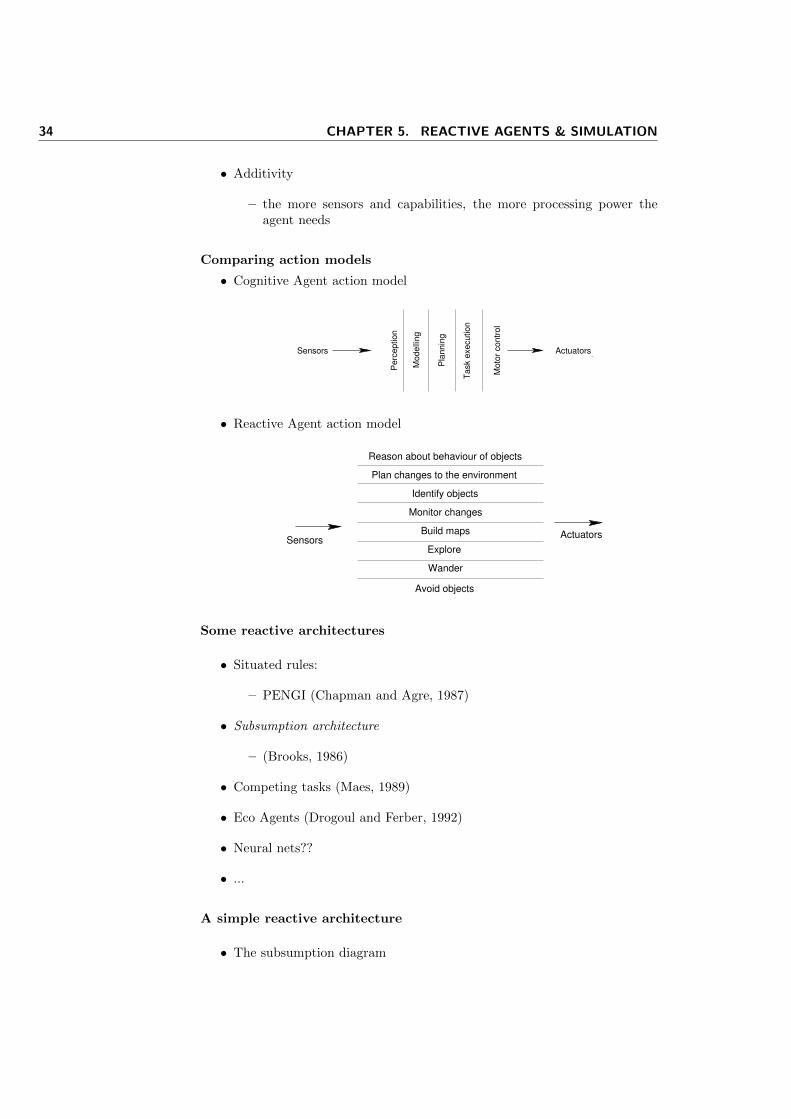
Comparing action models
• Cognitive Agent action model
Sensors Actuators
Perc
eption
Modelli
ng
Pla
nnin
g
Task e
xecution
Moto
r contr
ol
• Reactive Agent action model
Plan changes to the environment
Identify objects
Monitor changes
Explore
Build maps
Avoid objects
Wander
Reason about behaviour of objects
SensorsActuators
Some reactive architectures
• Situated rules:
– PENGI (Chapman and Agre, 1987)
• Subsumption architecture
– (Brooks, 1986)
• Competing tasks (Maes, 1989)
• Eco Agents (Drogoul and Ferber, 1992)
• Neural nets??
• ...
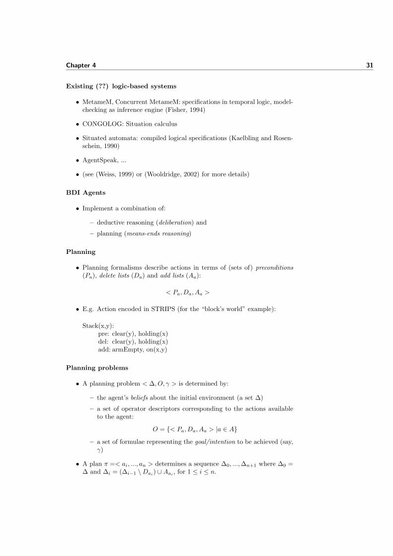
A simple reactive architecture
• The subsumption diagram
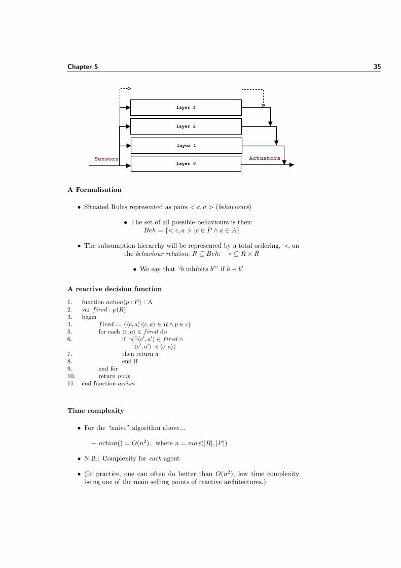
Chapter 5 35
layer 0
layer 1
layer 2
layer 3
Sensors Actuators
A Formalisation
• Situated Rules represented as pairs < c, a > (behaviours)
• The set of all possible behaviours is then:Beh = {< c, a > |c ∈ P ∧ a ∈ A}
• The subsumption hierarchy will be represented by a total ordering, ≺, onthe behaviour relation, R ⊆ Beh: ≺ ⊆ R×R
• We say that “b inhibits b′” if b ≺ b′
A reactive decision function
1. function action(p : P ) : A2. var fired : ℘(R)3. begin4. fired := {〈c, a〉|〈c, a〉 ∈ R ∧ p ∈ c}5. for each 〈c, a〉 ∈ fired do6. if ¬(∃〈c′, a′〉 ∈ fired ∧
〈c′, a′〉 ≺ 〈c, a〉)7. then return a8. end if9. end for10. return noop11. end function action
Time complexity
• For the “naive” algorithm above...
– action() = O(n2), where n = max(|R|, |P |)
• N.B.: Complexity for each agent
• (In practice, one can often do better than O(n2), low time complexitybeing one of the main selling points of reactive architectures.)
36 CHAPTER 5. REACTIVE AGENTS & SIMULATION
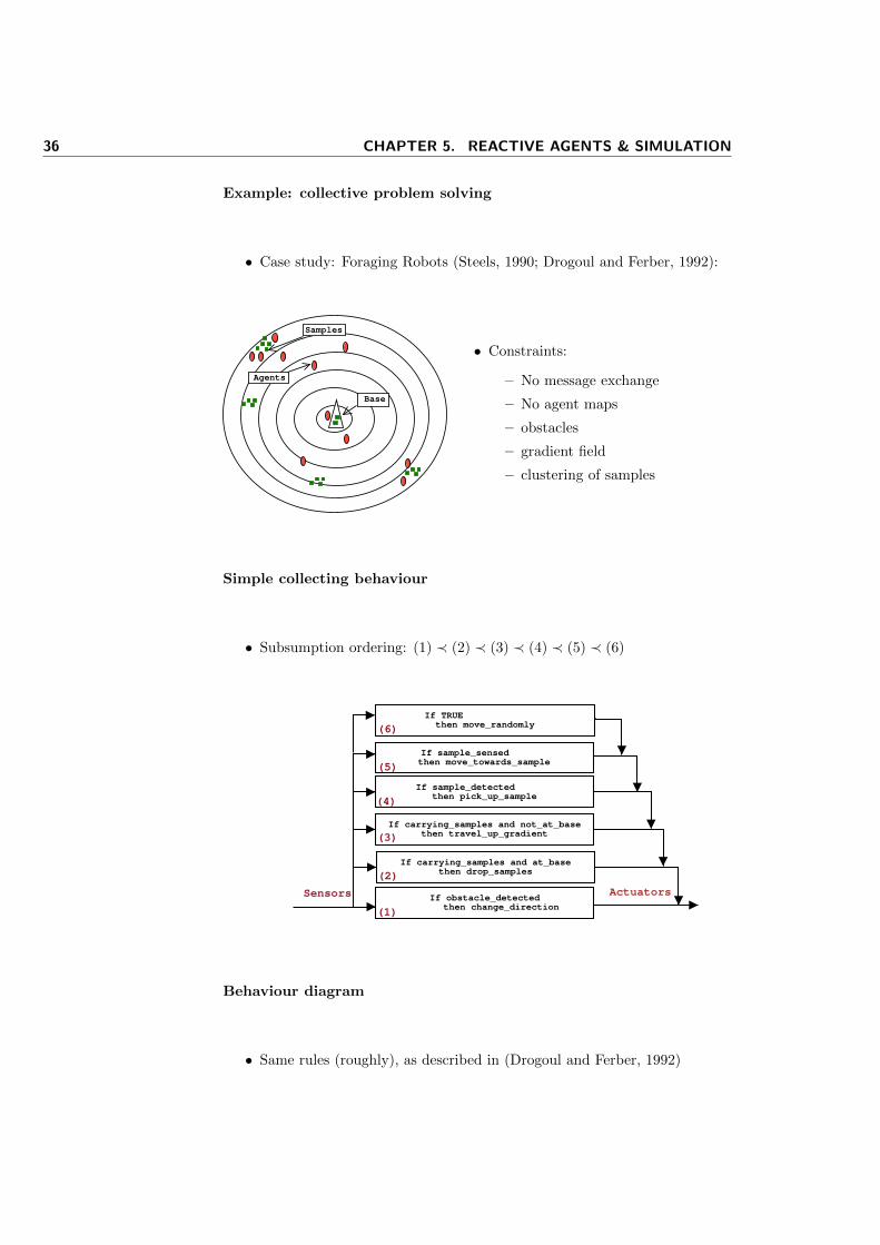
Example: collective problem solving
• Case study: Foraging Robots (Steels, 1990; Drogoul and Ferber, 1992):
z
Samples
Agents
Base
• Constraints:
– No message exchange
– No agent maps
– obstacles
– gradient field
– clustering of samples
Simple collecting behaviour
• Subsumption ordering: (1) ≺ (2) ≺ (3) ≺ (4) ≺ (5) ≺ (6)
If obstacle_detected then change_direction
If carrying_samples and at_basethen drop_samples
If carrying_samples and not_at_basethen travel_up_gradient
If sample_detected then pick_up_sample
If TRUE then move_randomly
Sensors Actuators
(1)
(2)
(3)
(4)
(5)
If sample_sensed then move_towards_sample
(5)
(6)
Behaviour diagram
• Same rules (roughly), as described in (Drogoul and Ferber, 1992)
Chapter 5 37
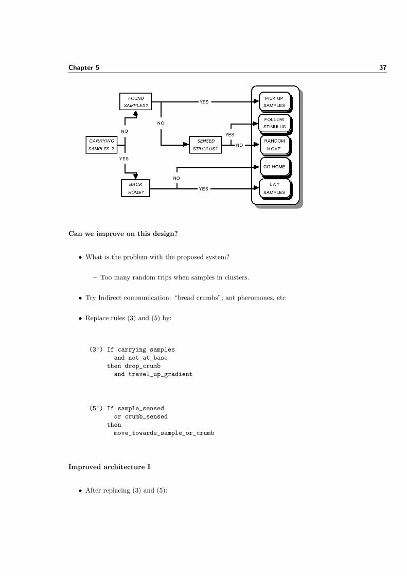
Can we improve on this design?
• What is the problem with the proposed system?
– Too many random trips when samples in clusters.
• Try Indirect communication: “bread crumbs”, ant pheromones, etc
• Replace rules (3) and (5) by:
(3’) If carrying samples
and not_at_base
then drop_crumb
and travel_up_gradient
(5’) If sample_sensed
or crumb_sensed
then
move_towards_sample_or_crumb
Improved architecture I
• After replacing (3) and (5):
38 CHAPTER 5. REACTIVE AGENTS & SIMULATION
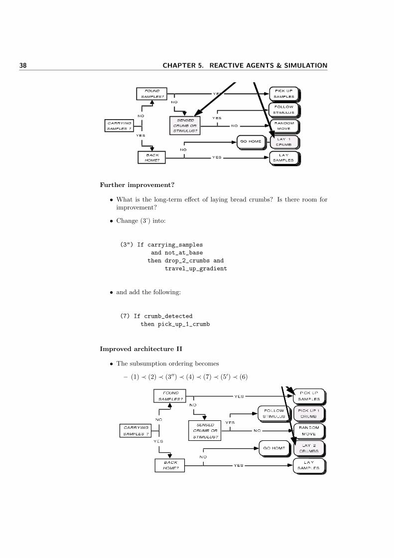
Further improvement?
• What is the long-term effect of laying bread crumbs? Is there room forimprovement?
• Change (3’) into:
(3") If carrying_samples
and not_at_base
then drop_2_crumbs and
travel_up_gradient
• and add the following:
(7) If crumb_detected
then pick_up_1_crumb
Improved architecture II
• The subsumption ordering becomes
– (1) ≺ (2) ≺ (3′′) ≺ (4) ≺ (7) ≺ (5′) ≺ (6)
Chapter 5 39
Advantages of this approach
• Low time (and space) complexity
• Robustness
• Better performance
– (near optimal in some cases)
– problems when the agent population is large
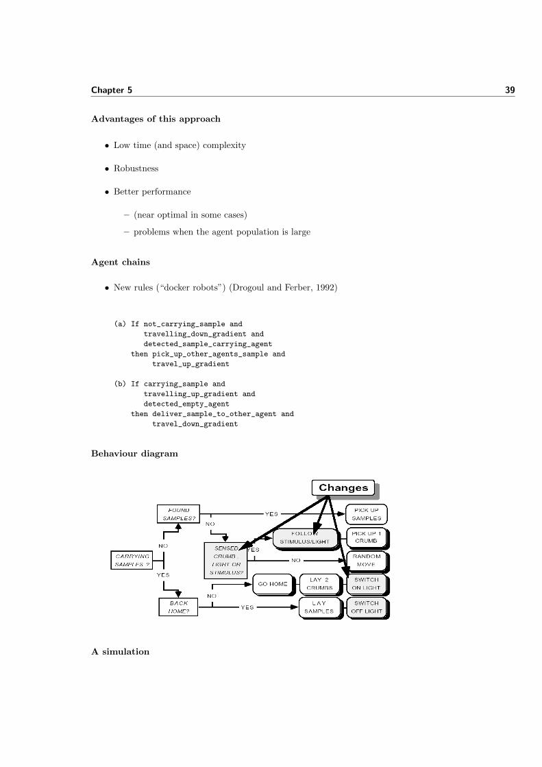
Agent chains
• New rules (“docker robots”) (Drogoul and Ferber, 1992)
(a) If not_carrying_sample and
travelling_down_gradient and
detected_sample_carrying_agent
then pick_up_other_agents_sample and
travel_up_gradient
(b) If carrying_sample and
travelling_up_gradient and
detected_empty_agent
then deliver_sample_to_other_agent and
travel_down_gradient
Behaviour diagram
A simulation
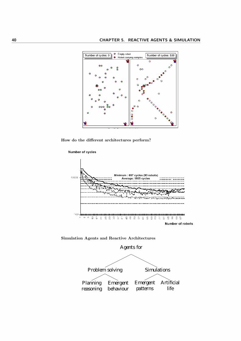
40 CHAPTER 5. REACTIVE AGENTS & SIMULATION
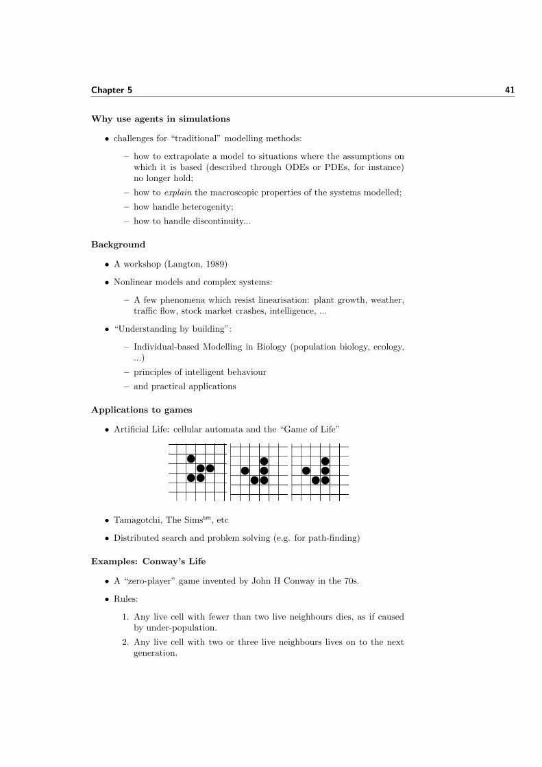
How do the different architectures perform?
Simulation Agents and Reactive Architectures
Agents for
Problem solving
Planningreasoning
Emergentbehaviour
Simulations
Emergentpatterns
Artificiallife
Chapter 5 41
Why use agents in simulations
• challenges for “traditional” modelling methods:
– how to extrapolate a model to situations where the assumptions onwhich it is based (described through ODEs or PDEs, for instance)no longer hold;
– how to explain the macroscopic properties of the systems modelled;
– how handle heterogenity;
– how to handle discontinuity...
Background
• A workshop (Langton, 1989)
• Nonlinear models and complex systems:
– A few phenomena which resist linearisation: plant growth, weather,traffic flow, stock market crashes, intelligence, ...
• “Understanding by building”:
– Individual-based Modelling in Biology (population biology, ecology,...)
– principles of intelligent behaviour
– and practical applications
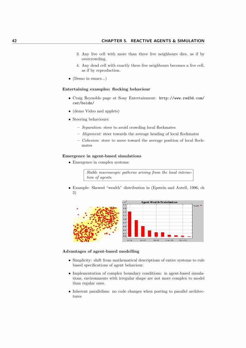
Applications to games
• Artificial Life: cellular automata and the “Game of Life”
• Tamagotchi, The Simstm, etc
• Distributed search and problem solving (e.g. for path-finding)
Examples: Conway’s Life
• A “zero-player” game invented by John H Conway in the 70s.
• Rules:
1. Any live cell with fewer than two live neighbours dies, as if causedby under-population.
2. Any live cell with two or three live neighbours lives on to the nextgeneration.
42 CHAPTER 5. REACTIVE AGENTS & SIMULATION
3. Any live cell with more than three live neighbours dies, as if byovercrowding.
4. Any dead cell with exactly three live neighbours becomes a live cell,as if by reproduction.
• (Demo in emacs...)
Entertaining examples: flocking behaviour
• Craig Reynolds page at Sony Entertainment: http://www.red3d.com/
cwr/boids/
• (demo Video and applets)
• Steering behaviours:
– Separation: steer to avoid crowding local flockmates
– Alignment: steer towards the average heading of local flockmates
– Cohesion: steer to move toward the average position of local flock-mates
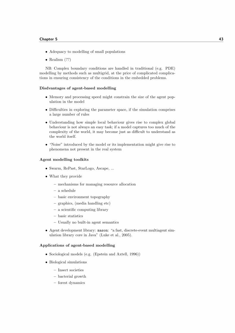
Emergence in agent-based simulations
• Emergence in complex systems:
Stable macroscopic patterns arising from the local interac-tion of agents.
• Example: Skewed “wealth” distribution in (Epstein and Axtell, 1996, ch2)
Advantages of agent-based modelling
• Simplicity: shift from mathematical descriptions of entire systems to rulebased specifications of agent behaviour.
• Implementation of complex boundary conditions: in agent-based simula-tions, environments with irregular shape are not more complex to modelthan regular ones.
• Inherent parallelism: no code changes when porting to parallel architec-tures
Chapter 5 43
• Adequacy to modelling of small populations
• Realism (??)
NB: Complex boundary conditions are handled in traditional (e.g. PDE)modelling by methods such as multigrid, at the price of complicated complica-tions in ensuring consistency of the conditions in the embedded problems.
Disdvantages of agent-based modelling
• Memory and processing speed might constrain the size of the agent pop-ulation in the model
• Difficulties in exploring the parameter space, if the simulation comprisesa large number of rules
• Understanding how simple local behaviour gives rise to complex globalbehaviour is not always an easy task; if a model captures too much of thecomplexity of the world, it may become just as difficult to understand asthe world itself.
• “Noise” introduced by the model or its implementation might give rise tophenomena not present in the real system
Agent modelling toolkits
• Swarm, RePast, StarLogo, Ascape, ...
• What they provide
– mechanisms for managing resource allocation
– a schedule
– basic environment topography
– graphics, (media handling etc)
– a scientific computing library
– basic statistics
– Usually no built-in agent semantics
• Agent development library: mason: “a fast, discrete-event multiagent sim-ulation library core in Java” (Luke et al., 2005).
Applications of agent-based modelling
• Sociological models (e.g. (Epstein and Axtell, 1996))
• Biological simulations
– Insect societies
– bacterial growth
– forest dynamics
44 CHAPTER 5. REACTIVE AGENTS & SIMULATION
• Molecule interaction in artificial chemistry
• Traffic simulations
• Computer networks (see http://www.crd.ge.com/~bushsf/ImperishNets.html, for instance)
RePast: A (Pure) Java Simulator
• Repast is an acronym for REcursive Porous Agent Simulation Toolkit.
“Our goal with Repast is to move beyond the representation ofagents as discrete, self-contained entities in favor of a view of so-cial actors as permeable, interleaved and mutually defining, withcascading and recombinant motives.”
From the Repast web site
• ??????
Two simulations: 1 - Mouse Traps
• A demonstration of “nuclear fission”:
– Lay a bunch of mousetraps on the floor in a regular grid, and loadeach mousetrap with two ping pong balls.
– Drop one ping pong ball in the middle...
• A discrete-event simulation that demonstrates the dynamic schedulingcapabilities of Repast
• The agent programmer defines:
– an agent (MouseTrap)
– a model (MouseTrapModel)
Two simulations: 2 - Heat Bugs
• “(...) an example of how simple agents acting only on local informationcan produce complex global behaviour”.
• Agents: HeatBugs which absorb and expel heat
• Model: HeatBugsModel has a spatial property, heat, which diffuses andevaporates over time. (green dots represent HeatBugs, brighter red rep-resents warmer spots of the world.)
• A HeatBug has an ideal temperature and will move about the space at-tempting to achieve this ideal temperature.

6Practical: Multiagent Simulations in Java
6.1 Goals
In this lab we will take a look at a Java-based simulation environment calledRepast1, run two simple demos, learn the basics of how to build a simulation,and analyse and modify a simulation of economic agents (Epstein and Axtell,1996).
6.2 Setting up the environment
The simulation software you will need may have already been installed on themachines in the IET Lab. If not, please download Repast, version 32 from thecourse’s software repository3. And uncompress it to a suitable directory (folder)in your user area. In the rest of this document we will refer to the location ofthe Repast directory (folder) on these machines as REPAST_HOME.
The libraries you will need in order to compile and run the simulations arelocated in REPAST_HOME/ and REPAST_HOME/lib/. These include simulation-specific packages (such as repast.jar), CERN’s scientific computing libraries(colt.jar), chart plotting libraries (plot.jar, jchart.jar), etc.
The source code for the original demos is located in REPAST_HOME/demo/.You will find modified versions of some of the demos for use in this lab4 on thecourse website. Just download and uncompress them into the same folder whereyou uncompressed repast3.1.tgz, so that your directory tree will look like this:
--|
|
|-- repast3.1/
|
|-- simlab-0.8/ --|
|--- bugs/
1Repast is an acronym for REcursive Porous Agent Simulation Toolkit.2Newer versions might work as well, but I haven’t tested them.3https://www.scss.tcd.ie/~luzs/t/cs7032/sw/repast3.1.tgz4http://www.scss.tcd.ie/~luzs/t/cs7032/sw/simlab-0.8.tar.gz
46 CHAPTER 6. PRACTICAL: MULTIAGENT SIMULATIONS IN JAVA
|--- mousetraps/
|--- sscape-2.0-lab/
The demos can be run via the shell scripts (Unix) or batch files (Windows)provided. These scripts are set so that they will “find” the repast libraries inthe above directory structure. If you uncompress repast to a different location,you will have to set the REPAST_HOME variable manually in these scripts so thatit points to the location of repast on your machine.
Documentation for the simulation (REPAST) and scientific computing (COLT)API’s is available in javadoc format in REPAST_HOME/docs/{api,colt}, respec-tively. Further information on how to build and run simulations in Repast canbe found in
REPAST_HOME/docs/how_to/how_to.html.
6.3 Running two demos
We will start by running two demos originally developed to illustrate the Swarmsimulation environment and ported to Repast:
Mouse trap: a simple discrete-event simulation the illustrates the dynamicscheduling capabilities of Repast (and Swarm, the simulation system forwhich it was first developed). The source code contains detailed commen-tary explaining how the simulator and model work. Please take a closelook at it.
Heatbugs: an example of how simple agents acting only on local informa-tion can produce complex global behaviour. Each agent in this model isa ‘HeatBug’. The world (a 2D torus) has a spatial property, heat, whichdiffuses and evaporates over time. The environmental heat property is con-trolled in HeatSpace.java5. The world is displayed on a DisplaySurface6
which depicts agents as green dots and warmer spots of the environmentas brighter red cells. The class HeatBugsModel7 sets up the environment,initialise the simulation parameters (which you can change via the GUI)distributes the agents on it and schedules actions to be performed at eachtime ‘tick’. Agents release a certain amount of heat per iteration. Theyhave an ideal temperature, and assess at each step their level of ‘unhap-piness’ with their temperature at that step. Locally, since no agent canproduce enough heat on his own to make them happy, agents seek tominimise their individual unhappiness by moving to cells that will makethem happier in the immediate future. Although all agents act purelyon local ‘knowledge’, globally, the system can be seen as a distributedoptimisation algorithm that minimises average unhappiness. The originalcode has been modified so that it plots the average unhappiness for theenvironment, showing how it decreases over time.
5uchicago/src/repastdemos/heatBugs/HeatSpace.java6uchicago.src.sim.gui.DisplaySurface7uchicago.src.repastdemos.heatBugs.HeatBugsModel
Chapter 6 47
In order to run a demo, simply, cd to its directory (created by uncompressingthe lab archive), and use run.sh (or run.bat). If you want to modify thesimulations, and use compile.sh8 (or compile.bat) to recompile the code.
The purpose of running these simulations is to get acquainted with the simu-lation environment and get an idea of what it can do. So, feel free to experimentwith different parameters, options available through the GUI, etc. Details onhow to use the GUI can be found in the How-To documentation:
REPAST_HOME/how_to/simstart.html
6.4 Simulating simple economic ecosystems
Now we will explore the SugarScape demo in some detail. The demo is a par-tial implementation of the environment described in chapter 2 of (Epstein andAxtell, 1996). The growth rule Gα (page 23), the movement rule M (page 25),and the replacement rule R (PAGE 32) have been implemented.
A slightly modified version of the original demo is available in the archiveyou downloaded for the first part of this lab, in sscape-2.0-lab/. Shell scriptscompile.sh and run.sh contain the classpath settings you will need in orderto compile and run the simulation. Remember that if you are not usingthe repast3.1 distribution provided or if the distribution has not beenuncompressed as described above, you will need to modify the scripts (.batfiles) so that variable REPAST_HOME points to the right place.
6.4.1 Brief description of the sscape simulation
At the top level, the directory sscape-2.0-lab/* contains, in addition to thescripts, an (ASCII) description of the “sugar landscape”: sugarspace.pgm.Open this file with your favourite editor and observe that it is filled with digits(0-4) which represent the distribution of “food” on the environment.
The source code for the simulation is in sugarscape/*.java9. All Repastsimulations must contain a model class, which takes care of setting up the sim-ulation environment, and at least one agent class. The file SugarModel.java
contains an implementation of a model class, whereas SugarAgent.java andSugarSpace.java implement simple agents. Note that in this simulation, as isoften the case, the environment is also conceptualised as an agent, whose onlybehaviour in this case is described by the growth rule.
6.4.2 Exercises
These are some ideas for exercises involving the sscape simulation. Please answer(at least) three of the questions below and submit your answers by the end ofnext week.
1. Modify the topography of the environment by changing sugarscape.pgm
(copy the original file into, say, sugarscape.old first). Make four hillsinstead of two, or a valley, etc. What effect does the new shape of theworld have on the system dynamics?
8For emacs+JDEE users, there is a prj.el file in bugs which you may find useful.9uchicago/src/sim/sugarscape/*.java
48 CHAPTER 6. PRACTICAL: MULTIAGENT SIMULATIONS IN JAVA
2. What causes the uneven wealth distribution we see in the original simu-lation? Is it the agent death and replacement rule R? Is it the unevendistribution of food in sugarspace.pgm? Is it the variance in maximumage, or metabolism or vision? Pick one or two parameters of the modelwith the replacement rule and see how their variance affects the wealthdistribution.
3. Modify SugarModel.java so that it also displays a time series of agentpopulation. How does the population vary over time, if the default pa-rameters are used? Why?
4. Reset the initial parameters so that the initial agent population decreases,asymptotically approaching the environment’s carrying capacity (you mightwant to change the replacement rule and maximum death age, for in-stance). What carrying capacity (Epstein and Axtell, 1996, see pages30-31) values do you obtain for the original maximum values of agentmetabolism and vision?
5. Do an experiment on how the final carrying capacity of the system varieswith the initial population. Write down a hypothesis, then design an ex-periment to test that hypothesis by varying the initial population size.Draw a graph of the result, evaluate the hypothesis, and draw conclu-sions10.
6. Do an experiment to discover the effects of maximum metabolism andvision on agent survival.
10Exerxise suggested by N. Minar in an introduction to his implementation of the Sug-arScape in the SWARM toolkit (Minar, , now apparently offline)
7Swarm intelligence: Ant Colony Optimisation
Simulating problem solving?
• Can simulation be used to improve distributed (agent-based) problem solv-ing algorithms?
• Yes: directly, in a supervised fashion (e.g. Neural Nets “simulators”)
• But also, indirectly, via exploration & experimental parameter tuning
• Case Study: Ant Colony Optimisation Heuristics (Dorigo et al., 1996;Dorigo and Di Caro, 1999)
• See also (Bonabeau et al., 2000) for a concise introduction (* recommendedreading)
More specifically, the case study presented in these notes illustrate an ap-plication of ant algorithms to the symmetric variant of the traveling salesmanproblem. Ant algorithms have, as we will see, been employed in a number ofoptimization problems, including network routing and protein folding. The tech-niques presented here aim for generality and certain theoretical goals rather thanperformance in any of these particular application areas. For a good overviewof variants, optimizations and heuristics, please consult (Dorigo and Di Caro,1999).
Biological Inspiration
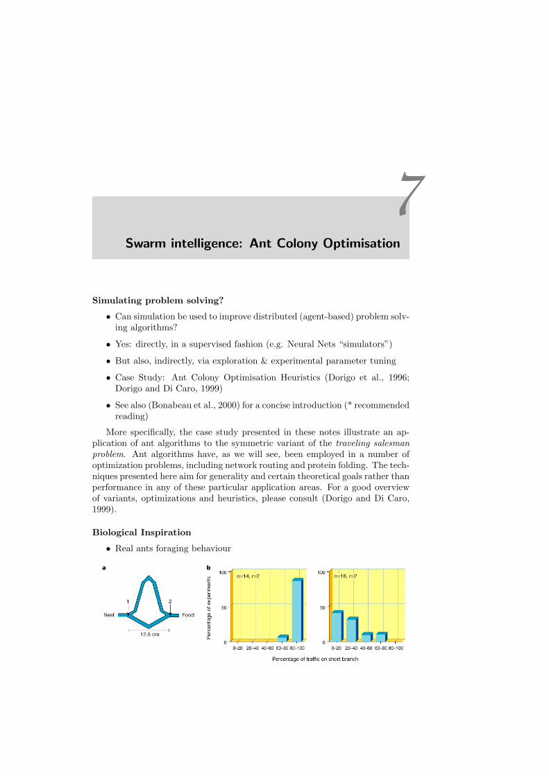
• Real ants foraging behaviour
50 CHAPTER 7. SWARM INTELLIGENCE: ANT COLONY OPTIMISATION
• long branch is r times longer than the short branch.
• left graph: branches presented simultaneously.
• right graph: shorter branch presented 30 mins. later
The gaphs show results of an actual experiment using real ants (Linepithemahumile). The role of pheromone plays is clear: it reinforces the ants’ preferencesfor a particular solution. If regarded as a system, the ant colony will “converge”to a poor solution if the short branch is presented too late (i.e. if the choice ofthe long branch is reinforced too strongly by the accummulated pheromone).
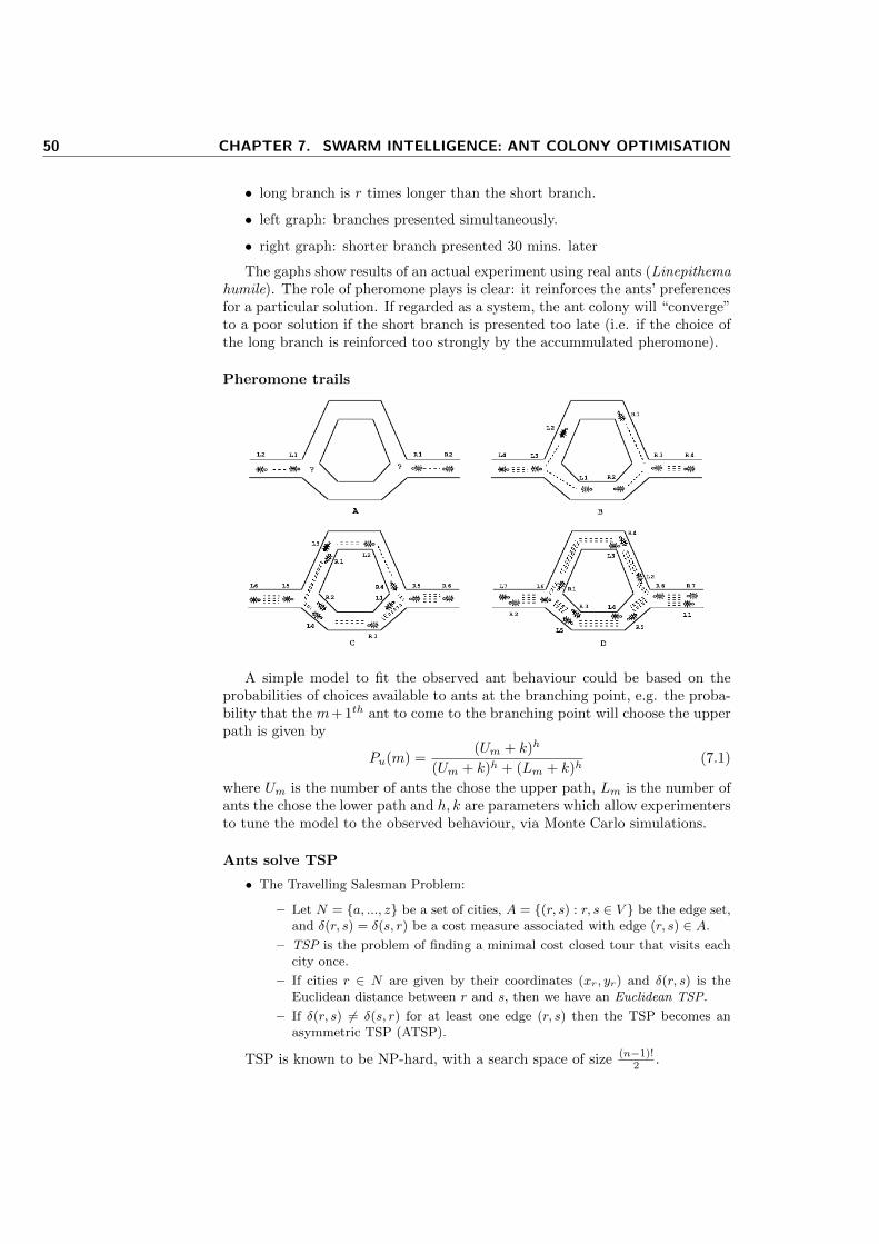
Pheromone trails
A simple model to fit the observed ant behaviour could be based on theprobabilities of choices available to ants at the branching point, e.g. the proba-bility that the m+1th ant to come to the branching point will choose the upperpath is given by
Pu(m) =(Um + k)h
(Um + k)h + (Lm + k)h(7.1)
where Um is the number of ants the chose the upper path, Lm is the number ofants the chose the lower path and h, k are parameters which allow experimentersto tune the model to the observed behaviour, via Monte Carlo simulations.
Ants solve TSP
• The Travelling Salesman Problem:
– Let N = {a, ..., z} be a set of cities, A = {(r, s) : r, s ∈ V } be the edge set,and δ(r, s) = δ(s, r) be a cost measure associated with edge (r, s) ∈ A.
– TSP is the problem of finding a minimal cost closed tour that visits eachcity once.
– If cities r ∈ N are given by their coordinates (xr, yr) and δ(r, s) is theEuclidean distance between r and s, then we have an Euclidean TSP.
– If δ(r, s) 6= δ(s, r) for at least one edge (r, s) then the TSP becomes anasymmetric TSP (ATSP).
TSP is known to be NP-hard, with a search space of size (n−1)!2 .
Chapter 7 51
A Simple Ant Algorithm for TSP
I n i t i a l i z ewhi l e ( ! End condit ion ){ /∗ c a l l the se ‘ i t e r a t i o n s ’ ∗/
p o s i t i o n each ant on a nodewhi l e ( ! a l l a n t s b u i l t c o m p l e t e s o l u t i o n ){ /∗ c a l l the se ‘ s teps ’ ∗/
f o r ( each ant ){
ant a p p l i e s a s t a t e t r a n s i t i o n r u l e toinc r ementa l l y bu i ld a s o l u t i o n
}}apply l o c a l ( per ant ) pheromone update r u l eapply g l o b a l pheromone update r u l e
}
Characteristics of Artificial Ants
• Similarities with real ants:
– They form a colony of cooperating individuals
– Use of pheromone for stigmergy (i.e. “stimulation of workers by thevery performance they have achieved” (Dorigo and Di Caro, 1999))
– Stochastic decision policy based on local information (i.e. no looka-head)
Dissimilarities with real ants
• Artificial Ants in Ant Algorithms keep internal state (so they wouldn’tqualify as purely reactive agents either)
• They deposit amounts of pheromone directly proportional to the qualityof the solution (i.e. the length of the path found)
• Some implementations use lookahead and backtracking as a means of im-proving search performance
Environmental differences
• Artificial ants operate in discrete environments (e.g. they will “jump”from city to city)
• Pheromone evaporation (as well as update) are usually problem-dependant
• (most algorithms only update pheromone levels after a complete tour hasbeen generated)
52 CHAPTER 7. SWARM INTELLIGENCE: ANT COLONY OPTIMISATION
ACO Meta heuristic
1 acoMetaHeur i s t i c ( )2 whi le ( ! t e r m i n a t i o n C r i t e r i a S a t i s f i e d )3 { / ∗ b e g i n s c h e d u l e A c t i v i t i e s ∗ /
4 antGenerat ionAndActivity ( )5 pheromoneEvaporation ( )6 daemonActions ( ) # opt i ona l #7 } / ∗ e n d s c h e d u l e a c t i v i t i e s ∗ /
1 antGenerat ionAndActivity ( )2 whi le ( ava i l ab l eR e so u r c e s )3 {4 scheduleCreationOfNewAnt ( )5 newActiveAnt ( )6 }
Ant lifecycle
1 newActiveAnt ( )2 i n i t i a l i s e ( )3 M := updateMemory ( )4 whi le ( cu r r en tS ta t e 6= t a r g e t S t a t e ) {5 A := readLocalRoutingTable ( )6 P := t r a n s i t i o n P r o b a b i l i t i e s (A,M, c o n s t r a i n t s )7 next := app lyDec i s i onPo l i cy (P, c o n s t r a i n t s )8 move( next )9 i f ( onlineStepByStepPheromoneUpdate ) {
10 depositPheromoneOnVisitedArc ( )11 updateRoutingTable ( )12 }13 M := update In t e rna lS ta t e ( )14 } / ∗ e n d w h i l e ∗ /
15 i f ( delayedPheromoneUpdate ) {16 eva lua t eSo lu t i on ( )17 depositPheromoneOnAllVis itedArcs ( )18 updateRoutingTable ( )19 }
How do ants decide which path to take?
• A decision table is built which combines pheromone and distance (cost)information:
• Ai = [aij(t)]|Ni|, for all j in Ni, where:
aij(t) =[τij(t)]
α[ηij ]β∑
l∈Ni [τil(t)]α[ηil]β
(7.2)
• Ni: set of nodes accessible from i
• τij(t): pheromone level on edge (i, j) at iteration t
• ηij = 1δij
Chapter 7 53
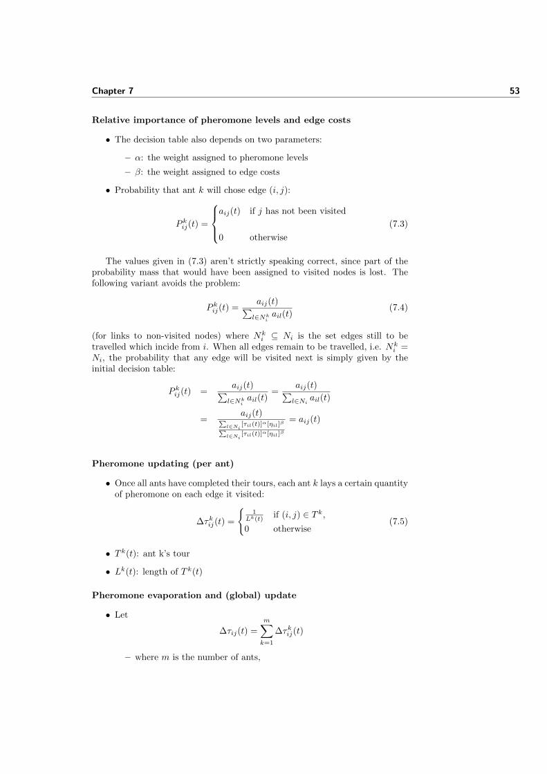
Relative importance of pheromone levels and edge costs
• The decision table also depends on two parameters:
– α: the weight assigned to pheromone levels
– β: the weight assigned to edge costs
• Probability that ant k will chose edge (i, j):
P kij(t) =
aij(t) if j has not been visited
0 otherwise
(7.3)
The values given in (7.3) aren’t strictly speaking correct, since part of theprobability mass that would have been assigned to visited nodes is lost. Thefollowing variant avoids the problem:
P kij(t) =aij(t)∑l∈Nki
ail(t)(7.4)
(for links to non-visited nodes) where Nki ⊆ Ni is the set edges still to be
travelled which incide from i. When all edges remain to be travelled, i.e. Nki =
Ni, the probability that any edge will be visited next is simply given by theinitial decision table:
P kij(t) =aij(t)∑l∈Nki
ail(t)=
aij(t)∑l∈Ni ail(t)
=aij(t)∑
l∈Ni[τil(t)]α[ηil]β∑
l∈Ni[τil(t)]α[ηil]β
= aij(t)
Pheromone updating (per ant)
• Once all ants have completed their tours, each ant k lays a certain quantityof pheromone on each edge it visited:
∆τkij(t) =
{1
Lk(t)if (i, j) ∈ T k,
0 otherwise(7.5)
• T k(t): ant k’s tour
• Lk(t): length of T k(t)
Pheromone evaporation and (global) update
• Let
∆τij(t) =
m∑k=1
∆τkij(t)
– where m is the number of ants,
54 CHAPTER 7. SWARM INTELLIGENCE: ANT COLONY OPTIMISATION
• and ρ ∈ (0, 1] be a pheromone decay coefficient
• The (per iteration) pheromone update rule is given by:
τij(t) = (1− ρ)τij(t′) + ∆τij(t) (7.6)
where t′ = t− 1
Parameter setting
• How do we choose appropriate values for the following parameters?
– α: the weight assigned to pheromone levels NB: if α = 0 only edgecosts (lengths) will be considered
– β: the weight assigned to edge costs NB: if β = 0 the search will beguided exclusively by pheromone levels
– ρ: the evaporation rate
– m: the number of ants
Exploring the parameter space
• Different parameters can be “empirically” tested using a multiagent sim-ulator such as Repast
• Vary the problem space
• Collect statistics
• Run benchmarks
• etc
Performance of ACO on TSP
• Ant algorithms perform better than the best known evolutionary com-putation technique (Genetic Algorithms) on the Asymmetric TravellingSalesman Problem (ATSP)
• ... and practically as well as Genetic Algorithms and Tabu Search onstandard TSP
• Good performance on other problems such as Sequential Ordering Prob-lem, Job Scheduling Problem, and Vehicle Routing Problem
Other applications
• Network routing (Caro and Dorigo, 1998) and load balancing (Heusseet al., 1998)
Chapter 7 55
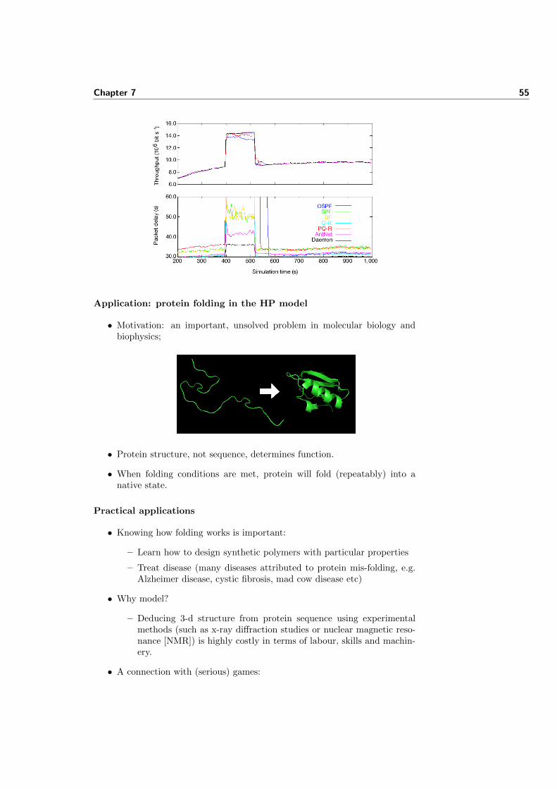
Application: protein folding in the HP model
• Motivation: an important, unsolved problem in molecular biology andbiophysics;
• Protein structure, not sequence, determines function.
• When folding conditions are met, protein will fold (repeatably) into anative state.
Practical applications
• Knowing how folding works is important:
– Learn how to design synthetic polymers with particular properties
– Treat disease (many diseases attributed to protein mis-folding, e.g.Alzheimer disease, cystic fibrosis, mad cow disease etc)
• Why model?
– Deducing 3-d structure from protein sequence using experimentalmethods (such as x-ray diffraction studies or nuclear magnetic reso-nance [NMR]) is highly costly in terms of labour, skills and machin-ery.
• A connection with (serious) games:
56 CHAPTER 7. SWARM INTELLIGENCE: ANT COLONY OPTIMISATION
– Fold.it: A Protein folding game...
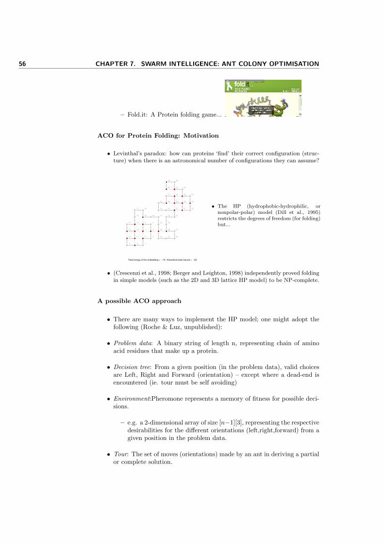
ACO for Protein Folding: Motivation
• Levinthal’s paradox: how can proteins ‘find’ their correct configuration (struc-ture) when there is an astronomical number of configurations they can assume?
1
2 3
4
56
789
10 11
1213
14 15
16
17 18
19 20 21
22
23
24 25 26
2728
29
30 31
323334
35 36
37 38
39 40
41 42
43
4445
4647
4849
50
Total energy of this embedding = −19 ; theoretical lower bound = −25
• The HP (hydrophobic-hydrophilic, ornonpolar-polar) model (Dill et al., 1995)restricts the degrees of freedom (for folding)but...
• (Crescenzi et al., 1998; Berger and Leighton, 1998) independently proved foldingin simple models (such as the 2D and 3D lattice HP model) to be NP-complete.
A possible ACO approach
• There are many ways to implement the HP model; one might adopt thefollowing (Roche & Luz, unpublished):
• Problem data: A binary string of length n, representing chain of aminoacid residues that make up a protein.
• Decision tree: From a given position (in the problem data), valid choicesare Left, Right and Forward (orientation) – except where a dead-end isencountered (ie. tour must be self avoiding)
• Environment:Pheromone represents a memory of fitness for possible deci-sions.
– e.g. a 2-dimensional array of size [n−1][3], representing the respectivedesirabilities for the different orientations (left,right,forward) from agiven position in the problem data.
• Tour: The set of moves (orientations) made by an ant in deriving a partialor complete solution.
Chapter 7 57
Ant behaviour
• State transition rule: How ant selects next move (left,right,forward)
– Exploitation:
∗ Greedy algorithm involve a lookahead (r ≥ 2) to gauge localbenefit of choosing a particular direction (benefit measured interms of additional HH contacts)
∗ Combine greedy algorithm with ‘intuition’ (pheromone), to de-rive overall cost measure
– Exploration: Pseudo-random (often biased) selection of an orienta-tion (help avoid local minima)
– Constraints:
∗ Resultant tour must be self avoiding.
∗ Look-ahead could help detect unpromising folding (e.g. two el-ements can be topological neighbours only when the number ofelements between them is even etc)
Pheromone update
• Local update: (optional)
– Can follow same approach as with TSP, by applying pheromone decayto edges as those edges are visited, to promote the exploration ofdifferent paths by subsequent ants during this iteration.
• Global update:
– Can also follow same approach as with TSP: Apply pheromone decay(evaporation!) to each edge in the decision tree (negative factor)
– Selection of ‘best’ candidate (best cost) and reinforcement of pheromoneon edges representing this decision
– Typically global updating rule will be iteration-best or global-best
Results
• Competitive with best-known algorithms (MCMC, GA, etc) in terms ofbest conformations found
• Can be slow and more resource-intensive.
• May be possible to combine ACO with techniques useb by approximationalgorithms (Hart and Istrail, 1995)
• Alternative approaches based on ACO have been proposed (Shmygelskaand Hoos, 2003).

8Practical: ACO simulation for TSP in Repast
8.1 Goals
In this practical you will implement an Ant Colony Optmisation (ACO) algo-rithm (Dorigo and Di Caro, 1999) for the Travelling Salesman Problem, andvisualise its performance through Repast.
8.2 Some code
In the course web site you will find some Java code for this practical1. Thiscode2 should provide you with the basics for implementing an ACO simulationusing Repast, namely: the basic model for the simulation (TSAModel3), a map(TSAWorld4) of the TSACity5s to be visited, backed by a Object2DTorus6 andset by TSAModel to be displayed onto an Object2DDisplay7. The display in-cludes methods for drawing the nodes (as green squares) the total amount ofpheromone on each path/link (in white) and the best path (in red). The linkdrawing method is set so that the more pheromone a link contains the moreclearly the link will be drawn.
You will also find a placeholder class for TravellingSalesAnt8 which youwill modify in order to implement the ACO meta-heuristic. The code containsdocumentation explaining how the simulation is structured.
The libraries you will need in order to compile and run this simulation aredistributed under the repast3 release and have been included in this lab’s tar filein their .jar packaging for convenience. They include simulation-specific pack-ages (such as repastj.jar), CERN’s scientific computing libraries (colt.jar),plotting libraries (plot.jar) and the trove high performance collections library.
1http://www.scss.tcd.ie/~luzs/t/cs7032/sw/tsa-0.7.tar.gz2The package is named “sim.tsa”, short for “Travelling Sales Ant”, after a project by Armin
Buch, a former student.3sim.tsa.TSAModel4sim.tsa.TSAWorld5sim.tsa.TSACity6uchicago.src.sim.space.Object2DTorus7uchicago.src.sim.gui.Object2DDisplay8sim.tsa.TravellingSalesAnt
60 CHAPTER 8. PRACTICAL: ACO SIMULATION FOR TSP IN REPAST
Emacs/JDEE users will find a prj.el9 file which can be used for compilationand running of the simulation under JDEE with a minor modification to thesetting of jde-global-classpath.
Bourne shell scripts and Windows “batch files” have been included for com-pilation (compile.sh and compile.bat) and stand-alone running of the simula-tion (run.sh, run.bat). They refer only to libraries included in the tar file andshould be easily translated into equivalent .bat files (i.e. by replacing colons bysemi-colons and forward slashes by backslashes etc).
Although the above described code template is provided, you are free toimplement your own ACO algorithm for TSP from scratch. You may evenuse a different simulation platform, such as MASON10, which offers similarfunctionality to Repast.
8.3 Exercises
From the list of exercises below, please attempt exercise 1, plus one of theremaining exercises of your choice.
1. Implement the behaviour of a an active ant (see newActiveAnt() in thelecture notes) by modifying (implementing, in fact) methods step() andstep2() in TravellingSalesAnt.java.
2. Modify the model so that the program allows you to save and load citymaps (i.e. specific instances of TSP) so that you can compare the per-formance of the algorithm across several runs under different parametersettings. A database of symmetrical TSP (and related problems) and theirbest known tours can be found at the Univeity of Heidelberg’s TSPLIB11.
3. Experiment with different parameters settings (e.g. number of ants, dis-tance weight, pheromone weight, amount of pheromone) and report brieflyon how the algorithm performs.
4. TSAModel differs from the algorithm describe in class in that TSAModel
currently updates pheromone only after all ants have finished their tour.Try modifying the code so that each ant leaves its pheromone trail im-mediately after it completes its tour. What effect does that have on thesystem?
5. Can you devise a heuristic for identifying unpromising solutions and dy-namically tuning the ACO parameters in order to enable the algorithm toexplore a wider solution space?
8.3.1 Delivering the assignment
Please submit this assignemt (as usual) through blackboard, by the deadlinespecified in the blackboard assignment submission page. Any text should besubmitted either as plain text or in PDF format. No MSWord files, please.Code and text should be submitted as a single file in a compressed archiveformat (.tar.gz or .zip).
9sim/tsa/prj.el10http://cs.gmu.edu/~eclab/projects/mason/11http://comopt.ifi.uni-heidelberg.de/software/TSPLIB95/
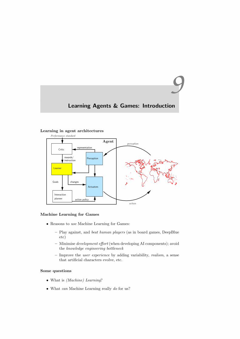
9Learning Agents & Games: Introduction
Learning in agent architectures
Agentperception
action
Actuators
Perception
Learner
changes
Performance standard
Criticrepresentation
rewards/instruction
Goals
Interaction
planner action policy
Machine Learning for Games
• Reasons to use Machine Learning for Games:
– Play against, and beat human players (as in board games, DeepBlueetc)
– Minimise development effort (when developing AI components); avoidthe knowledge engineering bottleneck
– Improve the user experience by adding variability, realism, a sensethat artificial characters evolve, etc.
Some questions
• What is (Machine) Learning?
• What can Machine Learning really do for us?
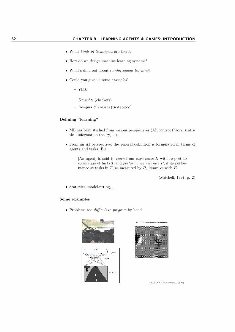
62 CHAPTER 9. LEARNING AGENTS & GAMES: INTRODUCTION
• What kinds of techniques are there?
• How do we design machine learning systems?
• What’s different about reinforcement learning?
• Could you give us some examples?
– YES:
– Draughts (checkers)
– Noughts & crosses (tic-tac-toe)
Defining “learning”
• ML has been studied from various perspectives (AI, control theory, statis-tics, information theory, ...)
• From an AI perspective, the general definition is formulated in terms ofagents and tasks. E.g.:
[An agent] is said to learn from experience E with respect tosome class of tasks T and performance measure P , if its perfor-mance at tasks in T , as measured by P , improves with E.
(Mitchell, 1997, p. 2)
• Statistics, model-fitting, ...
Some examples
• Problems too difficult to program by hand
(ALVINN (Pomerleau, 1994))
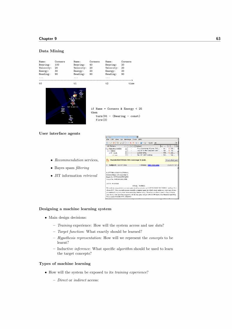
Chapter 9 63
Data Mining
Name: Corners Name: Corners Name: CornersBearing: 100 Bearing: 40 Bearing: 20Velocity: 20 Velocity: 20 Velocity: 20Energy: 30 Energy: 20 Energy: 20Heading: 90 Heading: 90 Heading: 90... ... ...---------------------------------------------------------------->t0 t1 t2 time
if Name = Corners & Energy < 25
then
turn(91 - (Bearing - const)
fire(3)
User interface agents
• Recommendation services,
• Bayes spam filtering
• JIT information retrieval
Designing a machine learning system
• Main design decisions:
– Training experience: How will the system access and use data?
– Target function: What exactly should be learned?
– Hypothesis representation: How will we represent the concepts to belearnt?
– Inductive inference: What specific algorithm should be used to learnthe target concepts?
Types of machine learning
• How will the system be exposed to its training experience?
– Direct or indirect access:
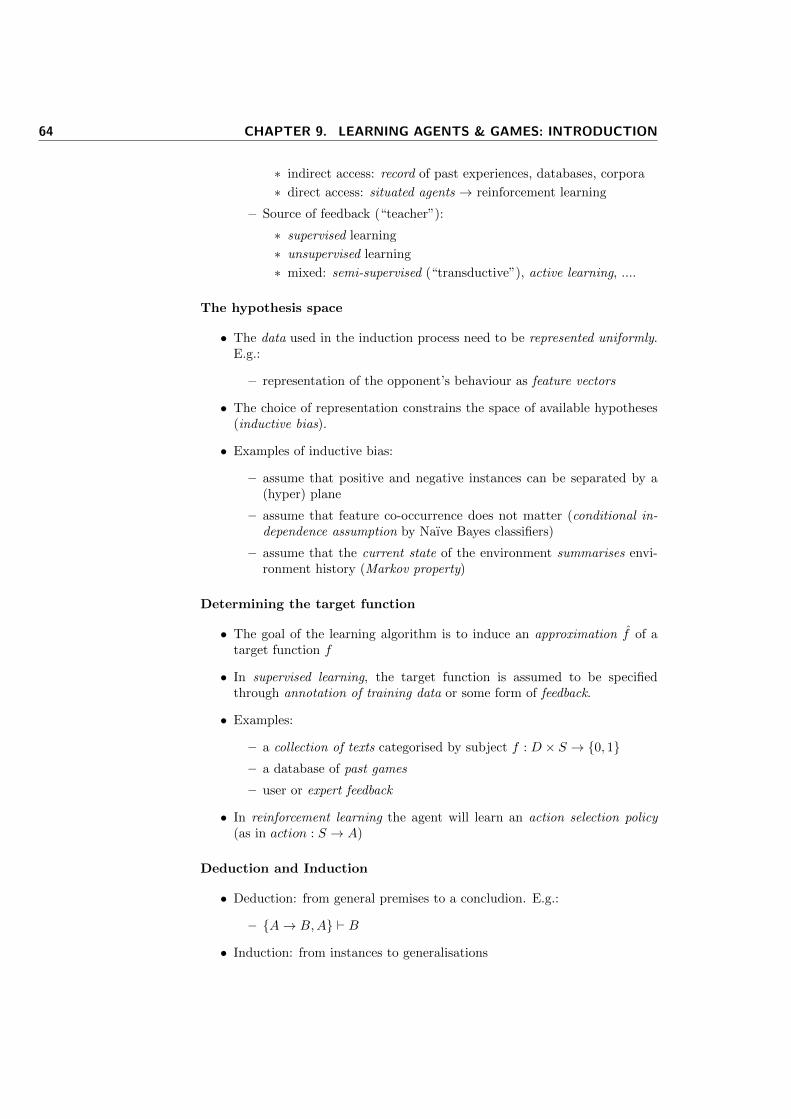
64 CHAPTER 9. LEARNING AGENTS & GAMES: INTRODUCTION
∗ indirect access: record of past experiences, databases, corpora
∗ direct access: situated agents → reinforcement learning
– Source of feedback (“teacher”):
∗ supervised learning
∗ unsupervised learning
∗ mixed: semi-supervised (“transductive”), active learning, ....
The hypothesis space
• The data used in the induction process need to be represented uniformly.E.g.:
– representation of the opponent’s behaviour as feature vectors
• The choice of representation constrains the space of available hypotheses(inductive bias).
• Examples of inductive bias:
– assume that positive and negative instances can be separated by a(hyper) plane
– assume that feature co-occurrence does not matter (conditional in-dependence assumption by Naıve Bayes classifiers)
– assume that the current state of the environment summarises envi-ronment history (Markov property)
Determining the target function
• The goal of the learning algorithm is to induce an approximation f of atarget function f
• In supervised learning, the target function is assumed to be specifiedthrough annotation of training data or some form of feedback.
• Examples:
– a collection of texts categorised by subject f : D × S → {0, 1}– a database of past games
– user or expert feedback
• In reinforcement learning the agent will learn an action selection policy(as in action : S → A)
Deduction and Induction
• Deduction: from general premises to a concludion. E.g.:
– {A→ B,A} ` B
• Induction: from instances to generalisations
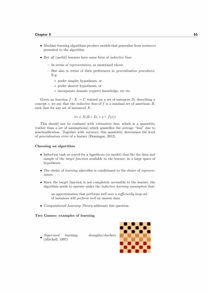
Chapter 9 65
• Machine learning algorithms produce models that generalise from instancespresented to the algorithm
• But all (useful) learners have some form of inductive bias:
– In terms of representation, as mentioned above,
– But also in terms of their preferences in generalisation procedures.E.g:
∗ prefer simpler hypotheses, or
∗ prefer shorter hypotheses, or
∗ incorporate domain (expert) knowledge, etc etc
Given an function f : X → C trained on a set of instances Dc describing aconcept c, we say that the inductive bias of f is a minimal set of assertions B,such that for any set of instanced X:
∀x ∈ X(B ∧Dc ∧ x ` f(x))
This should not be confused with estimation bias, which is a quantitity(rather than a set of assumptions) which quantifies the average “loss” due tomisclassification. Together with variance, this quantitity determines the levelof generalisation error of a learner (Domingos, 2012).
Choosing an algorithm
• Induction task as search for a hypothesis (or model) that fits the data andsample of the target function available to the learner, in a large space ofhypotheses
• The choice of learning algorithm is conditioned to the choice of represen-tation
• Since the target function is not completely accessible to the learner, thealgorithm needs to operate under the inductive learning assumption that:
an approximation that performs well over a sufficiently large setof instances will perform well on unseen data
• Computational Learning Theory addresses this question.
Two Games: examples of learning
• Supervised learning: draughts/checkers(Mitchell, 1997)
66 CHAPTER 9. LEARNING AGENTS & GAMES: INTRODUCTION
• Reinforcement learning: noughts and crosses(Sutton and Barto, 1998) X
X
X
O O
XO
• Task? (target function, data representation) Training experience? Perfor-mance measure?
A target for a draughts learner
• Learn.... f : Board→ Action or f : Board→ R
• But how do we label (evaluate) the training experience?
• Ask an expert?
• Derive values from a rational strategy:
– if b is a final board state that is won, then f(b) = 100
– if b is a final board state that is lost, then f(b) = −100
– if b is a final board state that is drawn, then f(b) = 0
– if b is a not a final state in the game, then f(b) = f(b′), where b′ isthe best final board state that can be achieved starting from b andplaying optimally until the end of the game.
• How feasible would it be to implement these strategies?
– Hmmmm... Not feasible...
Hypotheses and Representation
• The choice of representation (e.g. logical formulae, decision tree, neuralnet architecture) constrains the hypothesis search space.
• A representation scheme: linear combination of board features:
f(b) = w0 + w1 · bp(b) + w2 · rp(b) + w3 · bk(b)
+w4 · rk(b) + w5 · bt(b) + w6 · rt(b)
• where:
– bp(b): number of black pieces on board b
– rp(b): number of red pieces on b
– bk(b): number of black kings on b
– rk(b): number of red kings on b
– bt(b): number of red pieces threatened by black
– rt(b): number of black pieces threatened by red
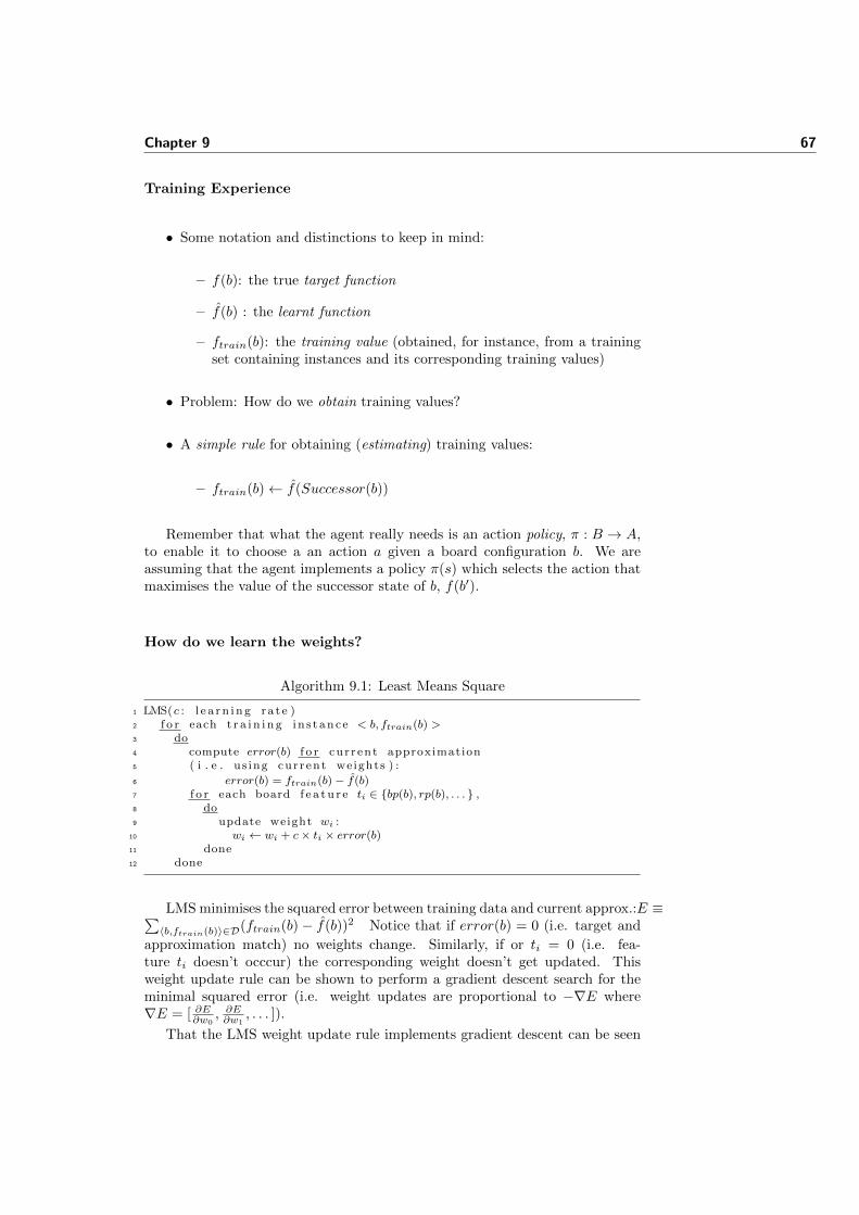
Chapter 9 67
Training Experience
• Some notation and distinctions to keep in mind:
– f(b): the true target function
– f(b) : the learnt function
– ftrain(b): the training value (obtained, for instance, from a trainingset containing instances and its corresponding training values)
• Problem: How do we obtain training values?
• A simple rule for obtaining (estimating) training values:
– ftrain(b)← f(Successor(b))
Remember that what the agent really needs is an action policy, π : B → A,to enable it to choose a an action a given a board configuration b. We areassuming that the agent implements a policy π(s) which selects the action thatmaximises the value of the successor state of b, f(b′).
How do we learn the weights?
Algorithm 9.1: Least Means Square
1 LMS(c : l e a r n i n g ra t e )2 f o r each t r a i n i n g in s t ance < b, ftrain(b) >3 do4 compute error(b) f o r cur r ent approximation5 ( i . e . us ing cur rent weights ) :
6 error(b) = ftrain(b)− f(b)7 f o r each board f e a t u r e ti ∈ {bp(b), rp(b), . . . } ,8 do9 update weight wi :
10 wi ← wi + c× ti × error(b)11 done12 done
LMS minimises the squared error between training data and current approx.:E ≡∑〈b,ftrain(b)〉∈D(ftrain(b) − f(b))2 Notice that if error(b) = 0 (i.e. target and
approximation match) no weights change. Similarly, if or ti = 0 (i.e. fea-ture ti doesn’t occcur) the corresponding weight doesn’t get updated. Thisweight update rule can be shown to perform a gradient descent search for theminimal squared error (i.e. weight updates are proportional to −∇E where∇E = [ ∂E∂w0
, ∂E∂w1, . . . ]).
That the LMS weight update rule implements gradient descent can be seen
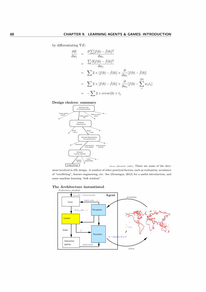
68 CHAPTER 9. LEARNING AGENTS & GAMES: INTRODUCTION
by differentiating ∇E:
∂E
∂wi=
∂∑
[f(b)− f(b)]2
∂wi
=
∑∂[f(b)− f(b)]2
∂wi
=∑
2× [f(b)− f(b)]× ∂
∂wi[f(b)− f(b)]
=∑
2× [f(b)− f(b)]× ∂
∂wi[f(b)−
|D|∑i
wjtj ]
= −∑
2× error(b)× tj
Design choices: summary
Determine
Target Function
Determine Representation
of Learned Function
Determine Type
of Training Experience
Determine
Learning Algorithm
Games against self
Games against experts Table of correct
moves
Linear functionof six features
Artificial neural network
Polynomial
Gradient descent
Board Ý value
BoardÝ move
Completed Design
...
...
Linear programming
...
...
(from (Mitchell, 1997)) These are some of the deci-
sions involved in ML design. A number of other practical factors, such as evaluation, avoidance
of “overfitting”, feature engineering, etc. See (Domingos, 2012) for a useful introduction, and
some machine learning “folk wisdom”.
The Architecture instantiated
perception
action
Critic
Learner
Goals
Interaction
planner action policy
Actuators
changes
Perception
representation
Performance standard
Agent
rewards/instruction
(bp(b), rp(b), . . .)
ftrain(b) := f(successor(b)
(b, ftrain(b), . . .)
f
initial board
π∗ = arg maxπ f(s),∀s
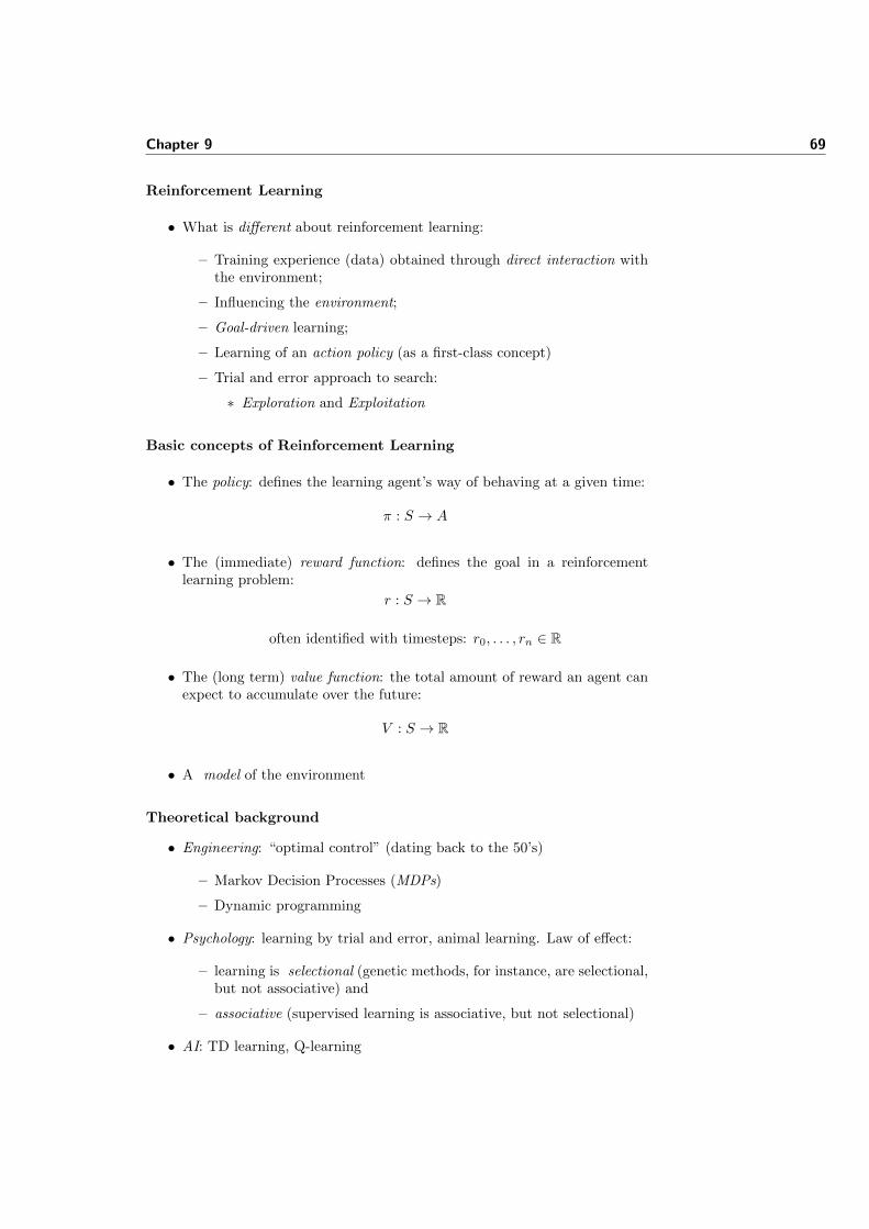
Chapter 9 69
Reinforcement Learning
• What is different about reinforcement learning:
– Training experience (data) obtained through direct interaction withthe environment;
– Influencing the environment;
– Goal-driven learning;
– Learning of an action policy (as a first-class concept)
– Trial and error approach to search:
∗ Exploration and Exploitation
Basic concepts of Reinforcement Learning
• The policy: defines the learning agent’s way of behaving at a given time:
π : S → A
• The (immediate) reward function: defines the goal in a reinforcementlearning problem:
r : S → R
often identified with timesteps: r0, . . . , rn ∈ R
• The (long term) value function: the total amount of reward an agent canexpect to accumulate over the future:
V : S → R
• A model of the environment
Theoretical background
• Engineering: “optimal control” (dating back to the 50’s)
– Markov Decision Processes (MDPs)
– Dynamic programming
• Psychology: learning by trial and error, animal learning. Law of effect:
– learning is selectional (genetic methods, for instance, are selectional,but not associative) and
– associative (supervised learning is associative, but not selectional)
• AI: TD learning, Q-learning
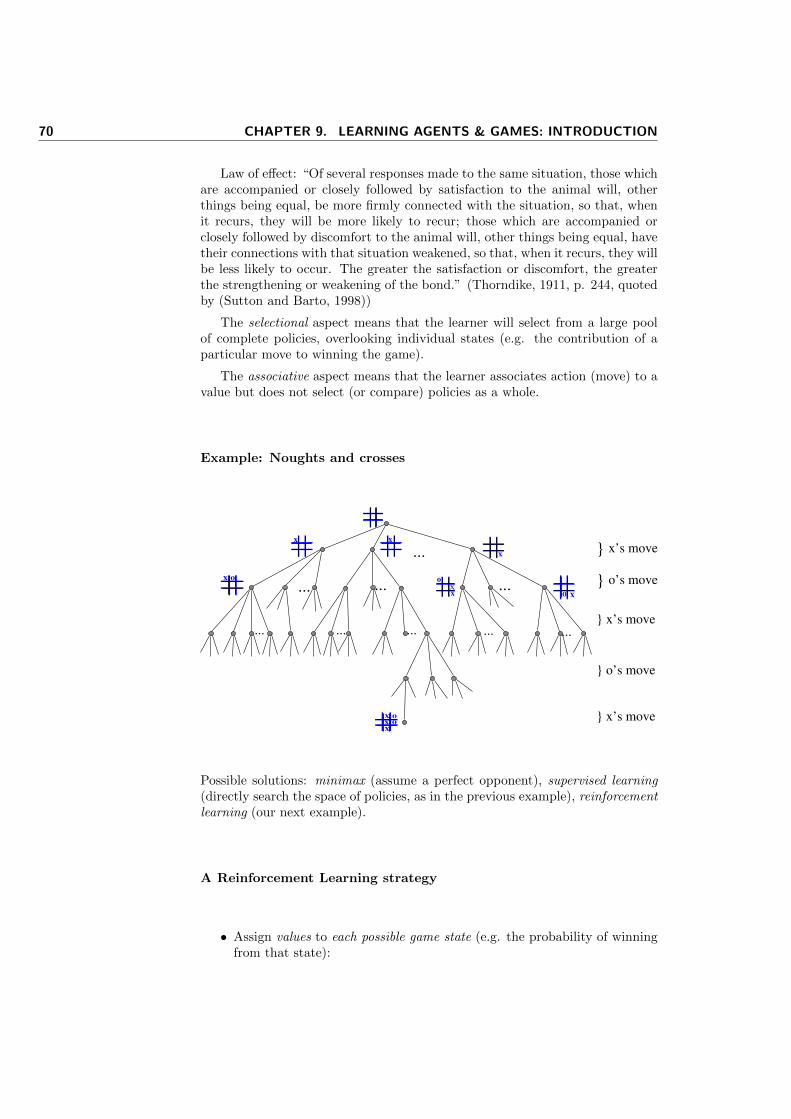
70 CHAPTER 9. LEARNING AGENTS & GAMES: INTRODUCTION
Law of effect: “Of several responses made to the same situation, those whichare accompanied or closely followed by satisfaction to the animal will, otherthings being equal, be more firmly connected with the situation, so that, whenit recurs, they will be more likely to recur; those which are accompanied orclosely followed by discomfort to the animal will, other things being equal, havetheir connections with that situation weakened, so that, when it recurs, they willbe less likely to occur. The greater the satisfaction or discomfort, the greaterthe strengthening or weakening of the bond.” (Thorndike, 1911, p. 244, quotedby (Sutton and Barto, 1998))
The selectional aspect means that the learner will select from a large poolof complete policies, overlooking individual states (e.g. the contribution of aparticular move to winning the game).
The associative aspect means that the learner associates action (move) to avalue but does not select (or compare) policies as a whole.
Example: Noughts and crosses
Possible solutions: minimax (assume a perfect opponent), supervised learning(directly search the space of policies, as in the previous example), reinforcementlearning (our next example).
A Reinforcement Learning strategy
• Assign values to each possible game state (e.g. the probability of winningfrom that state):
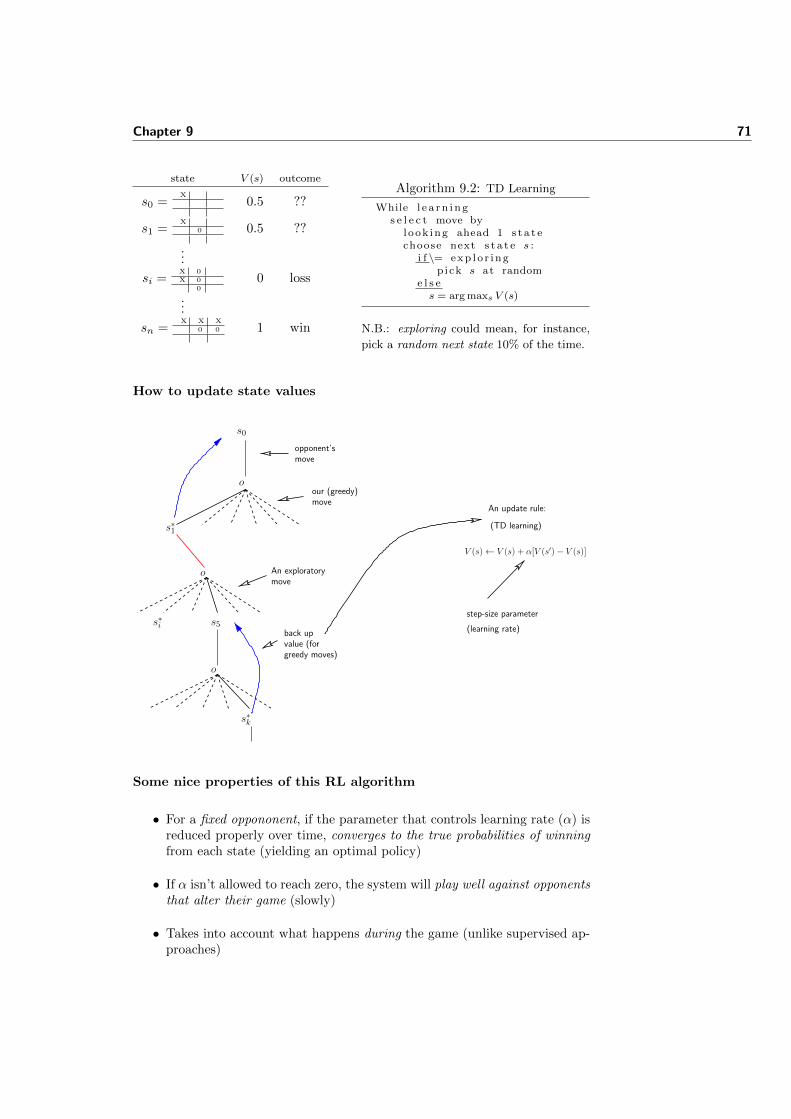
Chapter 9 71
state V (s) outcome
s0 =X
0.5 ??
s1 =X
0 0.5 ??
...
si =X 0
X 0
0
0 loss
...
sn =X X X
0 0 1 win
Algorithm 9.2: TD Learning
While l e a r n i n gs e l e c t move by
look ing ahead 1 s t a t echoose next s t a t e s :
i f \= exp lo r i ngpick s at random
e l s es = arg maxs V (s)
N.B.: exploring could mean, for instance,
pick a random next state 10% of the time.
How to update state values
s0
opponent’smove
o
s∗1
our (greedy)move
o
s∗i
An exploratorymove
s5
o
s∗k
back upvalue (forgreedy moves)
V (s)← V (s) + α[V (s′)− V (s)]
(TD learning)
An update rule:
step-size parameter
(learning rate)
Some nice properties of this RL algorithm
• For a fixed oppononent, if the parameter that controls learning rate (α) isreduced properly over time, converges to the true probabilities of winningfrom each state (yielding an optimal policy)
• If α isn’t allowed to reach zero, the system will play well against opponentsthat alter their game (slowly)
• Takes into account what happens during the game (unlike supervised ap-proaches)

72 CHAPTER 9. LEARNING AGENTS & GAMES: INTRODUCTION
What was not illustrated
• RL also applies to situations where there isn’t a clearly defined adversary(“games against nature”)
• RL also applies to non-episodic problems (i.e. rewards can be received atany time not only at the end of an episode such as a finished game)
• RL scales up well to games where the search space is (unlike our example)truly vast.
– See (Tesauro, 1994), for instance.
• Prior knowledge can also be incorporated
• Look-ahead isn’t always required
10Practical: Survey of game AI competitions
10.1 Goals
To learn about a Game AI competition (preferably one the is co-located with anAI or games conference). Give a short presentation describing the competition.The final course project will involve creating an entry for a competition to bechosen among the ones presented in class. The presentations can be done bygroups of 3 students.
10.2 What to do
1. Start by exploring some game-AI conference websites, such as the TheIEEE Conference on Computational Intelligence and Games1, The IEEEWorld Congress on Computational Intelligence2, or the AI and InteractiveDigital Entertainment Conference3, to see which competitions they host,how often they are held, requirements for participation etc. There are alsoweb sites that compile lists of such competitions.
2. Choose a game competition to present, and email me your choice andthe composition of your group. Groups should present different gamecompetitions, so choices will be recorded more or less on a 1st-come-1st-served basis.
3. Below is a list of possible games you might like to take a look at. Bearin mind that the deadlines for most competitions have already passed, soyour survey will basically look at past competitions (including the paperswritten by participants on the techniques they used). The expectation isthat the competition will run again in 2014. The list below is by no meanseshaustive, and is probably a bit out of date, so please feel free to searchfor Game AI competitions (here’s a sample search4).
1https://duckduckgo.com/?q=IEEE+Conference+on+Computational+Intelligence+and+
Games2http://ieee-wcci2014.org/3http://aiide.org4https://duckduckgo.com/?q=Game+AI+competitions
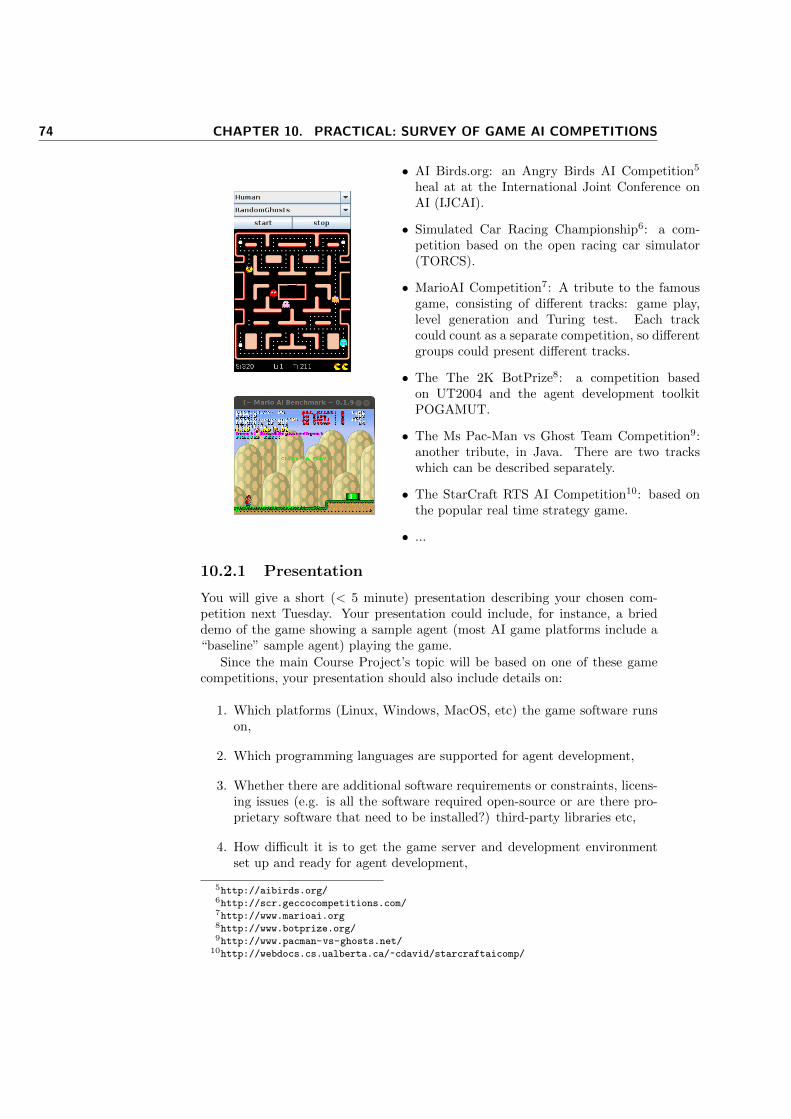
74 CHAPTER 10. PRACTICAL: SURVEY OF GAME AI COMPETITIONS
• AI Birds.org: an Angry Birds AI Competition5
heal at at the International Joint Conference onAI (IJCAI).
• Simulated Car Racing Championship6: a com-petition based on the open racing car simulator(TORCS).
• MarioAI Competition7: A tribute to the famousgame, consisting of different tracks: game play,level generation and Turing test. Each trackcould count as a separate competition, so differentgroups could present different tracks.
• The The 2K BotPrize8: a competition basedon UT2004 and the agent development toolkitPOGAMUT.
• The Ms Pac-Man vs Ghost Team Competition9:another tribute, in Java. There are two trackswhich can be described separately.
• The StarCraft RTS AI Competition10: based onthe popular real time strategy game.
• ...
10.2.1 Presentation
You will give a short (< 5 minute) presentation describing your chosen com-petition next Tuesday. Your presentation could include, for instance, a brieddemo of the game showing a sample agent (most AI game platforms include a“baseline” sample agent) playing the game.
Since the main Course Project’s topic will be based on one of these gamecompetitions, your presentation should also include details on:
1. Which platforms (Linux, Windows, MacOS, etc) the game software runson,
2. Which programming languages are supported for agent development,
3. Whether there are additional software requirements or constraints, licens-ing issues (e.g. is all the software required open-source or are there pro-prietary software that need to be installed?) third-party libraries etc,
4. How difficult it is to get the game server and development environmentset up and ready for agent development,
5http://aibirds.org/6http://scr.geccocompetitions.com/7http://www.marioai.org8http://www.botprize.org/9http://www.pacman-vs-ghosts.net/
10http://webdocs.cs.ualberta.ca/~cdavid/starcraftaicomp/

Chapter 10 75
5. Your assessment of how interesting the game/competition is in terms ofallowing us to explore AI techniques,
6. Whether there will be a competition next year (so we can perhaps enterit!)
Many of the game competitions above have been described in journal andconference papers (e.g. (Karakovskiy and Togelius, 2012), (Genesereth et al.,2005), (Shaker et al., 2011), (Loiacono et al., 2010), (Rohlfshagen and Lucas,2011)). There are also a number of papers describing various AI approaches em-ployed by participants in past competitions (e.g. these11). Feel free to explore.
11http://aibirds.org/symposium-on-ai-in-angry-birds/accepted-papers.html

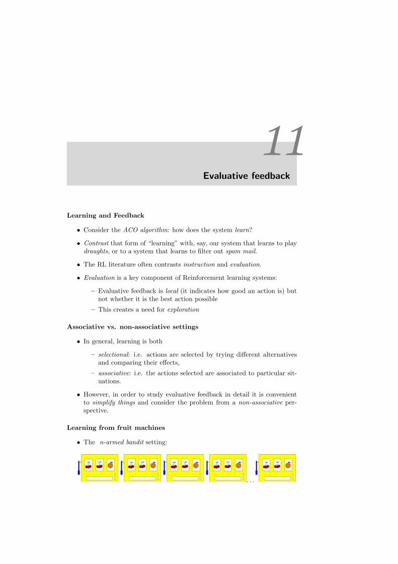
11Evaluative feedback
Learning and Feedback
• Consider the ACO algorithm: how does the system learn?
• Contrast that form of “learning” with, say, our system that learns to playdraughts, or to a system that learns to filter out spam mail.
• The RL literature often contrasts instruction and evaluation.
• Evaluation is a key component of Reinforcement learning systems:
– Evaluative feedback is local (it indicates how good an action is) butnot whether it is the best action possible
– This creates a need for exploration
Associative vs. non-associative settings
• In general, learning is both
– selectional: i.e. actions are selected by trying different alternativesand comparing their effects,
– associative: i.e. the actions selected are associated to particular sit-uations.
• However, in order to study evaluative feedback in detail it is convenientto simplify things and consider the problem from a non-associative per-spective.
Learning from fruit machines
• The n-armed bandit setting:
. . .
78 CHAPTER 11. EVALUATIVE FEEDBACK
• Choice of n actions (which yield numerical rewards drawn from a station-ary probability distribution)
– each action selection called a play
• Goal: maximise expected (long term) total reward or return.
– Strategy: concentrate plays on the best levers.
How to find the best plays
• Let’s distinguiguish between:
– reward, the immediate outcome of a play, and
– value, the expected (mean) reward of a play
• But how do we estimate values?
• We could keep a record of rewards ra1 , . . . , raka
for each chosen action a andestimate the value of choosing a at time t as
Qt(a) =ra1 + ra2 + · · ·+ raka
ka(11.1)
But how do we choose an action?
• We could be greedy and exploit our knowledge of Qt(a) to choose at anytime t the play with the highest estimated value.
• But this strategy will tend to neglect the estimates of non-greedy actions(which might have produced greater total reward in the long run).
• One could, alternatively, explore the space of actions by choosing, fromtime to time, a non-greedy action
Balancing exploitation and exploration
• The goal is to approximate the true value, Q(a) for each action
• Qt(a), given by equation (11.1) will converge to Q(a) as ka →∞ (Law ofLarge Numbers)
• So balancing exploration and exploitation is necessary...
• but finding the right balance can be tricky; many approaches rely on strongassumptions about the underlying distributions
• We will present a simpler alternative...
Chapter 11 79
A simple strategy
• The simplest strategy: choose action a∗ so that:
a∗ = arg maxa
Qt(a) (greedy selection) (11.2)
• A better simple strategy: ε-greedy methods:
– With probability 1− ε, exploit; i.e. choose a∗ according with (11.2)
– The rest of the time (probability ε) choose an action at random,uniformly
– A suitably small ε guarantees that all actions get explored sooner orlater (and the probability of selecting the optimal action converges togreater than 1− ε)
Exploring exploration at different rates
• The “10-armed testbed” (Sutton and Barto, 1998):
– 2000 randomly generated n-armed bandit tasks with n = 10.
– For each action, a, expected rewards Q(a) (the “true” expected values ofchoosing a) are selected from a normal (Gaussian) probability distributionN(0, 1)
– Immediate rewards ra1 , . . . , rak are similarly selected from N(Q(a), 1)
1 nArmedBanditTask <− function(n=10, s=2000)2 {3 qtrue <− rnorm(n)4 r <− matrix(nrow=s,ncol=n)5 for ( i in 1:n){6 r [, i ] <− rnorm(s,mean=qtrue[i])7 }8 return(r)9 }
Some empirical results
• Averaged results of 2000 rounds of 1000 plays each:
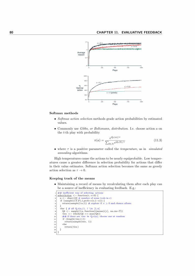
80 CHAPTER 11. EVALUATIVE FEEDBACK
= 0 (greedy)
= 0.01
0
0.5
1
1.5
Averagereward
0 250 500 750 1000
Plays
0%
20%
40%
60%
80%
100%
%Optimalaction
0 250 500 750 1000
= 0.1
Plays
= 0.01
= 0.1
Softmax methods
• Softmax action selection methods grade action probabilities by estimatedvalues.
• Commonly use Gibbs, or Boltzmann, distribution. I.e. choose action a onthe t-th play with probability
π(a) =eQt(a)/τ∑b∈A e
Qt(b)/τ(11.3)
• where τ is a positive parameter called the temperature, as in simulatedannealing algorithms.
High temperatures cause the actions to be nearly equiprobable. Low temper-atures cause a greater difference in selection probability for actions that differin their value estimates. Softmax action selection becomes the same as greedyaction selection as τ → 0.
Keeping track of the means
• Maintaining a record of means by recalculating them after each play canbe a source of inefficiency in evaluating feedback. E.g.:
1 ## inefficient way of selecting actions2 selectAction <− function(r, e=0) {3 n <− dim(r)[2] # number of arms (cols in r)4 if (sample(c(T,F),1,prob=c(e,1−e))) {5 return(sample(1:n,1)) # explore if e > 0 and chance allows6 }7 else { # all Q t(a i ), i \in [1, n]8 Qt <− sapply(1:n, function(i)mean(r[,i ], na.rm=T))9 ties <− which(Qt == max(Qt))
10 ## if there are ties in Q t(a); choose one at random11 if (length( ties )>1)12 return(sample(ties, 1))13 else14 return( ties )15 }16 }
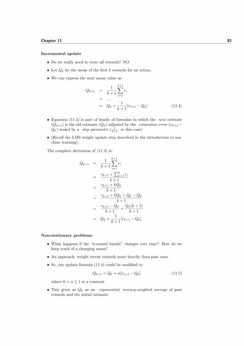
Chapter 11 81
Incremental update
• Do we really need to store all rewards? NO
• Let Qk be the mean of the first k rewards for an action,
• We can express the next mean value as
Qk+1 =1
k + 1
k+1∑i=1
ri
= . . .
= Qk +1
k + 1[rk+1 −Qk] (11.4)
• Equation (11.4) is part of family of formulae in which the new estimate(Qk+1) is the old estimate (Qk) adjusted by the estimation error (rk+1−Qk) scaled by a step parameter ( 1
k+1 , in this case)
• (Recall the LMS weight update step described in the introduction to ma-chine learning).
The complete derivation of (11.4) is:
Qk+1 =1
k + 1
k+1∑i=1
ri
=rk+1 +
∑k1=1 ri
k + 1
=rk+1 + kQk
k + 1
=rk+1 + kQk +Qk −Qk
k + 1
=rk+1 −Qkk + 1
+Qk(k + 1)
k + 1
= Qk +1
k + 1[rk+1 −Qk]
Non-stationary problems
• What happens if the “n-armed bandit” changes over time? How do wekeep track of a changing mean?
• An approach: weight recent rewards more heavily than past ones.
• So, our update formula (11.4) could be modified to
Qk+1 = Qk + α[rk+1 −Qk] (11.5)
where 0 < α ≤ 1 is a constant
• This gives us Qk as an exponential, recency-weighted average of pastrewards and the initial estimate
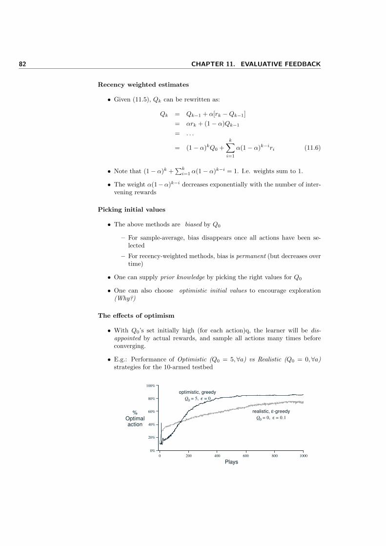
82 CHAPTER 11. EVALUATIVE FEEDBACK
Recency weighted estimates
• Given (11.5), Qk can be rewritten as:
Qk = Qk−1 + α[rk −Qk−1]
= αrk + (1− α)Qk−1
= . . .
= (1− α)kQ0 +
k∑i=1
α(1− α)k−iri (11.6)
• Note that (1− α)k +∑ki=1 α(1− α)k−i = 1. I.e. weights sum to 1.
• The weight α(1−α)k−i decreases exponentially with the number of inter-vening rewards
Picking initial values
• The above methods are biased by Q0
– For sample-average, bias disappears once all actions have been se-lected
– For recency-weighted methods, bias is permanent (but decreases overtime)
• One can supply prior knowledge by picking the right values for Q0
• One can also choose optimistic initial values to encourage exploration(Why?)
The effects of optimism
• With Q0’s set initially high (for each action)q, the learner will be dis-appointed by actual rewards, and sample all actions many times beforeconverging.
• E.g.: Performance of Optimistic (Q0 = 5,∀a) vs Realistic (Q0 = 0,∀a)strategies for the 10-armed testbed
0%
20%
40%
60%
80%
100%
%Optimalaction
0 200 400 600 800 1000
Plays
optimistic, greedy
Q0 = 5, = 0
realistic, ε-greedy
Q0 = 0, = 0.1
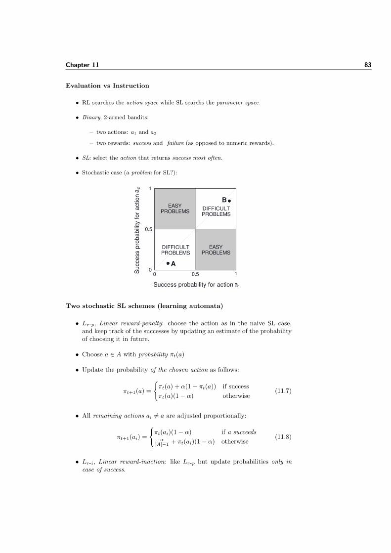
Chapter 11 83
Evaluation vs Instruction
• RL searches the action space while SL searchs the parameter space.
• Binary, 2-armed bandits:
– two actions: a1 and a2
– two rewards: success and failure (as opposed to numeric rewards).
• SL: select the action that returns success most often.
• Stochastic case (a problem for SL?):
0
1
0 1
B
A
EASYPROBLEMS
0.5
0.5
DIFFICULTPROBLEMS
DIFFICULTPROBLEMS
EASYPROBLEMS
Success probability for action a1
Suc
cess
prob
abili
tyfo
rac
tion
a 2
Two stochastic SL schemes (learning automata)
• Lr-p, Linear reward-penalty: choose the action as in the naive SL case,and keep track of the successes by updating an estimate of the probabilityof choosing it in future.
• Choose a ∈ A with probability πt(a)
• Update the probability of the chosen action as follows:
πt+1(a) =
{πt(a) + α(1− πt(a)) if success
πt(a)(1− α) otherwise(11.7)
• All remaining actions ai 6= a are adjusted proportionally:
πt+1(ai) =
{πt(ai)(1− α) if a succeedsα|A|−1 + πt(ai)(1− α) otherwise
(11.8)
• Lr-i, Linear reward-inaction: like Lr-p but update probabilities only incase of success.
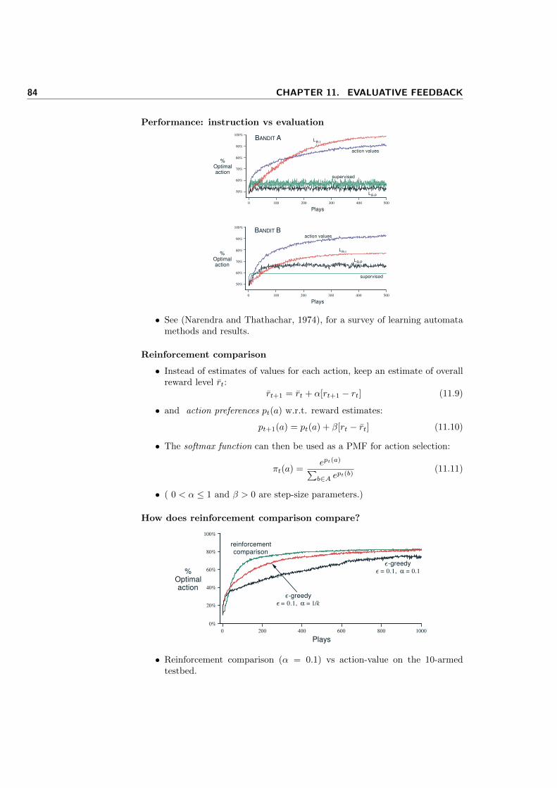
84 CHAPTER 11. EVALUATIVE FEEDBACK
Performance: instruction vs evaluation
90%
100%
%Optimalaction
0 100 200 300 400 500
Plays
%Optimalaction
0 100 200 300 400 500
BANDIT A
BANDIT B
action values
LR-I
LR-P
supervised
LR-I
action values
LR-P
supervised
Plays
80%
70%
60%
50%
90%
100%
80%
70%
60%
50%
• See (Narendra and Thathachar, 1974), for a survey of learning automatamethods and results.
Reinforcement comparison
• Instead of estimates of values for each action, keep an estimate of overallreward level rt:
rt+1 = rt + α[rt+1 − rt] (11.9)
• and action preferences pt(a) w.r.t. reward estimates:
pt+1(a) = pt(a) + β[rt − rt] (11.10)
• The softmax function can then be used as a PMF for action selection:
πt(a) =ept(a)∑b∈A e
pt(b)(11.11)
• ( 0 < α ≤ 1 and β > 0 are step-size parameters.)
How does reinforcement comparison compare?
0%
20%
40%
60%
80%
100%
%Optimalaction
0 200 400 600 800 1000
Plays
reinforcementcomparison
-greedy = 0.1, α = 1/k
-greedy = 0.1, α = 0.1
• Reinforcement comparison (α = 0.1) vs action-value on the 10-armedtestbed.
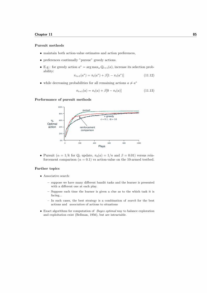
Chapter 11 85
Pursuit methods
• maintain both action-value estimates and action preferences,
• preferences continually ”pursue” greedy actions.
• E.g.: for greedy action a∗ = arg maxaQt+1(a), increase its selection prob-ability:
πt+1(a∗) = πt(a∗) + β[1− πt(a∗)] (11.12)
• while decreasing probabilities for all remaining actions a 6= a∗
πt+1(a) = πt(a) + β[0− πt(a)] (11.13)
Performance of pursuit methods
reinforcementcomparison
0%
20%
40%
60%
80%
100%
%Optimalaction
0 200 400 600 800 1000
Plays
-greedy
= 0.1, α = 1/k
pursuit
• Pursuit (α = 1/k for Qt update, π0(a) = 1/n and β = 0.01) versus rein-forcement comparison (α = 0.1) vs action-value on the 10-armed testbed.
Further topics
• Associative search:
– suppose we have many different bandit tasks and the learner is presentedwith a different one at each play.
– Suppose each time the learner is given a clue as to the which task it isfacing...
– In such cases, the best strategy is a combination of search for the bestactions and association of actions to situations
• Exact algorithms for computation of Bayes optimal way to balance explorationand exploitation exist (Bellman, 1956), but are intractable.

12Practical: Evaluating Evaluative Feedback
12.1 Goals
To replicate the experiments with the 10-armed testbed (Sutton and Barto,1998) presented in class1. To investigate different settings of the explorationvs exploitation dilemma. And to model a simple game as a MDP. The MDPmodelling part is unrelated to the R code given.
12.2 Some code
In the course web site you will find some code for this practical2. This filecontains functions that create an n-armed bandit task (makeNArmedBanditTask)and run the ε-greedy experiment described in the notes (runExperiment1).
The code is written in R, a programming environment for data analysis andgraphics which is freely available from the R project website3 (Venables andSmith, 2004). R has an Algol-like syntax which should make it relatively easy tolearn the basics. The code provided does not use any of the advanced featuresof the language, so it should be straightforward to extend and modify it. Ashort introduction to R4 is available through the course website. Only question2 requires some coding. However, you may use a programming language of yourchoice, or simply answer question 2 using pseudo-code.
The R code provided implements the basics of evaluative feedback as de-scribed in our lecture notes:
• function makeNArmedBanditTask(n,s) creates a matrix of s by n ran-domly sampled from normal distributions which represents s plays on n
machines (“arms”)
• function evalLearn(dset, e, tmax, q0) “learns” to evaluate feedbackfor dset (e.g. a 10-armed dataset generated as described above) by iter-ating up to tmax times, with greed factor e.
1http://www.scss.tcd.ie/~luzs/t/cs7032/1/efeedback-notes.pdf2http://www.scss.tcd.ie/~luzs/t/cs7032/1/sw/evfeedback.R3http://cran.r-project.org/4http://www.scss.tcd.ie/~luzs/t/cs7032/1/bib/R-intro.pdf

88 CHAPTER 12. PRACTICAL: EVALUATING EVALUATIVE FEEDBACK
• selectAction(avgr, e) selects an action that gives maximal rewardor an exploratory action, depending on the “greed” parameter e andupdateEstimate(old,target,step) updates the average rewards effi-ciently.
In addition, a sample function runExperiment1(...) is provided whichuses the above described code to run the first evaluative feedback simulationdescribed in the notes and plot the results.
12.3 Exercises
Do the following exercises, to be handed in next Tuesday:
1. run the initial evaluative feedback experiment for different settings of the“greed” parameter (ε), number of runs etc. Plot and compare the results.NB: \runExperiment1() does all that is needed, all you have to do is passdifferent parameters.
2. Extend or modify the R code given (or re-implement it in your languageof choice) so as to run at least one of the other settings described in thenotes: softmax action selection, optimistic initial estimates, reinforcementcomparison, etc. Alternatively (if you are not comfortable enough withR) you can simply describe the algorithm in pseudo-code.
3. Describe the robocode game as a Markov Decision process along the linesseen in the last lectures. In particular, outline a scheme for describing:
• the battle environment as a set of states (note that you will typicallyneed to simplify the state to a few variable, as we illustrated, forinstance, in our simplification of the draughts game).
• actions and
• a reward structure (for a robocode learner)
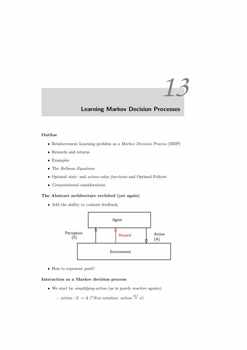
13Learning Markov Decision Processes
Outline
• Reinforcement Learning problem as a Markov Decision Process (MDP)
• Rewards and returns
• Examples
• The Bellman Equations
• Optimal state- and action-value functions and Optimal Policies
• Computational considerations
The Abstract architecture revisited (yet again)
• Add the ability to evaluate feedback:
Perception(S)
Action(A)
Environment
Agent
Reward
• How to represent goals?
Interaction as a Markov decision process
• We start by simplifying action (as in purely reactive agents):
– action : S → A (*New notation: actiondef= π)
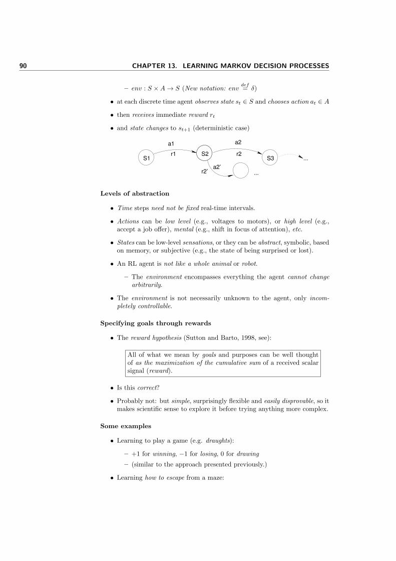
90 CHAPTER 13. LEARNING MARKOV DECISION PROCESSES
– env : S ×A→ S (New notation: envdef= δ)
• at each discrete time agent observes state st ∈ S and chooses action at ∈ A
• then receives immediate reward rt
• and state changes to st+1 (deterministic case)
...S2
S1 S3
a1 a2
r1 r2
a2’r2’ ...
Levels of abstraction
• Time steps need not be fixed real-time intervals.
• Actions can be low level (e.g., voltages to motors), or high level (e.g.,accept a job offer), mental (e.g., shift in focus of attention), etc.
• States can be low-level sensations, or they can be abstract, symbolic, basedon memory, or subjective (e.g., the state of being surprised or lost).
• An RL agent is not like a whole animal or robot.
– The environment encompasses everything the agent cannot changearbitrarily.
• The environment is not necessarily unknown to the agent, only incom-pletely controllable.
Specifying goals through rewards
• The reward hypothesis (Sutton and Barto, 1998, see):
All of what we mean by goals and purposes can be well thoughtof as the maximization of the cumulative sum of a received scalarsignal (reward).
• Is this correct?
• Probably not: but simple, surprisingly flexible and easily disprovable, so itmakes scientific sense to explore it before trying anything more complex.
Some examples
• Learning to play a game (e.g. draughts):
– +1 for winning, −1 for losing, 0 for drawing
– (similar to the approach presented previously.)
• Learning how to escape from a maze:
Chapter 13 91
– set the reward to zero until it escapes
– and +1 when it does.
• Recycling robot: +1 for each recyclable container collected, −1 if con-tainer isn’t recyclable, 0 for wandering, −1 for bumping into obstaclesetc.
Important points about specifying a reward scheme
• the reward signal is the place to specify what the agent’s goals are (giventhat the agent’s high-level goal is always to maximise its rewards)
• the reward signal is not the place to specify how to achieve such goals
• Where are rewards computed in our agent/environment diagram?
• Rewards and goals are outside the agent’s direct control, so they it makessense to assume they are computed by the environment!
From rewards to returns
• We define (expected) returns (Rt) to formalise the notion of rewards re-ceived in the long run.
• The simplest case:
Rt = rt+1 + rt+2 + · · ·+ rT (13.1)
where rt+1, . . . is the sequence of rewards received after time t, and T isthe final time step.
• What sort of agent/environment is this definition most appropriate for?
• Answer: episodic interactions (which break naturally into subsequences;e.g. a game of chess, trips through a maze, etc).
Non-episodic tasks
• Returns should be defined differently for continuing (aka non-episodic)tasks (i.e. T =∞).
• In such cases, the idea of discounting comes in handy:
Rt = rt+1 + γrt+2 + γ2rt+3 + · · · =∞∑k=0
γkrt+k+1 (13.2)
where 0 ≤ γ ≤ 1 is the discount rate
• Is this sum well defined?
• One can thus specify far-sighted or myopic agents by varying the discountrate γ.
If the rewards rk are bounded from above by some constant c and γ < 1,then the infinite sum in (13.2) is well defined, since it is an infinite sum of asequence bounded in absolute value by a decreasing geometric prograssion γc.
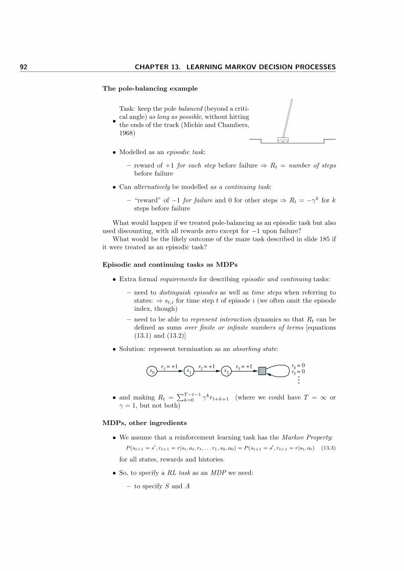
92 CHAPTER 13. LEARNING MARKOV DECISION PROCESSES
The pole-balancing example
•Task: keep the pole balanced (beyond a criti-cal angle) as long as possible, without hittingthe ends of the track (Michie and Chambers,1968)
• Modelled as an episodic task:
– reward of +1 for each step before failure ⇒ Rt = number of stepsbefore failure
• Can alternatively be modelled as a continuing task:
– “reward” of −1 for failure and 0 for other steps ⇒ Rt = −γk for ksteps before failure
What would happen if we treated pole-balancing as an episodic task but alsoused discounting, with all rewards zero except for −1 upon failure?
What would be the likely outcome of the maze task described in slide 185 ifit were treated as an episodic task?
Episodic and continuing tasks as MDPs
• Extra formal requirements for describing episodic and continuing tasks:
– need to distinguish episodes as well as time steps when referring tostates: ⇒ st,i for time step t of episode i (we often omit the episodeindex, though)
– need to be able to represent interaction dynamics so that Rt can bedefined as sums over finite or infinite numbers of terms [equations(13.1) and (13.2)]
• Solution: represent termination as an absorbing state:
r1
= +1s
0s
1
r2
= +1s
2
r3
= +1 r4
= 0
r5
= 0
• and making Rt =∑T−t−1k=0 γkrt+k+1 (where we could have T = ∞ or
γ = 1, but not both)
MDPs, other ingredients
• We assume that a reinforcement learning task has the Markov Property:
P (st+1 = s′, rt+1 = r|st, at, rt, . . . r1, s0, a0) = P (st+1 = s′, rt+1 = r|st, at) (13.3)
for all states, rewards and histories.
• So, to specify a RL task as an MDP we need:
– to specify S and A
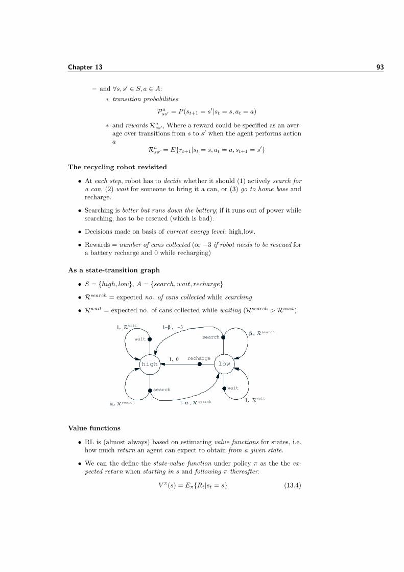
Chapter 13 93
– and ∀s, s′ ∈ S, a ∈ A:
∗ transition probabilities:
Pass′ = P (st+1 = s′|st = s, at = a)
∗ and rewards Rass′ , Where a reward could be specified as an aver-age over transitions from s to s′ when the agent performs actiona
Rass′ = E{rt+1|st = s, at = a, st+1 = s′}
The recycling robot revisited
• At each step, robot has to decide whether it should (1) actively search fora can, (2) wait for someone to bring it a can, or (3) go to home base andrecharge.
• Searching is better but runs down the battery; if it runs out of power whilesearching, has to be rescued (which is bad).
• Decisions made on basis of current energy level: high,low.
• Rewards = number of cans collected (or −3 if robot needs to be rescued fora battery recharge and 0 while recharging)
As a state-transition graph
• S = {high, low}, A = {search,wait, recharge}• Rsearch = expected no. of cans collected while searching
• Rwait = expected no. of cans collected while waiting (Rsearch > Rwait)
search
high low1, 0
1–β , –3
search
recharge
wait
wait
search1–α , R
β , R
search
α, R search
1, R wait
1, R wait
Value functions
• RL is (almost always) based on estimating value functions for states, i.e.how much return an agent can expect to obtain from a given state.
• We can the define the state-value function under policy π as the the ex-pected return when starting in s and following π thereafter:
V π(s) = Eπ{Rt|st = s} (13.4)
94 CHAPTER 13. LEARNING MARKOV DECISION PROCESSES
• Note that this implies averaging over probabilities of reaching future states,that is, P (st+1 = s′|st = s, at = a) over all t.
• We can also generalise the action function (policy) to π(s, a), returning theprobability of taking action a while in state s, which implies also averagingover actions.
The action-value function
• we can also define an action-value function to give the value of takingaction a in state s under a policy π:
Qπ(s, a) = Eπ{Rt|st = s, at = a} (13.5)
where Rt =∑∞k=0 γ
krt+k+1.
• Both vπ and Qπ can be estimated, for instance, through simulation (MonteCarlo methods):
– for each state s visited by following π, keep an average V π of returnsreceived from that point on.
– V π approaches V π as the number of times s is visited approaches ∞– Qπ can be estimated similarly.
The Bellman equation
• Value functions satisfy particular recursive relationships.
• For any policy π and any state s, the following consistency condition holds:
V π(s) = Eπ{Rt|st = s}
= Eπ{∞∑k=0
γkrt+k+1|st = s}
= Eπ{rt+1 + γ
∞∑k=0
γkrt+k+2|st = s}
=∑a
π(s, a)∑s′Pass′ [R
ass′ + γEπ{
∞∑k=0
γkrt+k+2|st+1 = s′}]
=∑a
π(s, a)∑s′Pass′ [R
ass′ + γV π(s′)] (13.6)
The value function for π is the unique solution for the set of linear equations(one per state) represented by (13.6).
Backup diagrams
• The Bellman equation for V π (13.6) expresses a relationship between thevalue of a state and the value of its successors.
• This can be depicted through backup diagrams
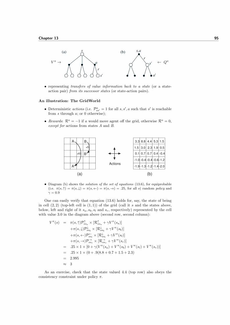
Chapter 13 95
V π →
s,as
a
s'
r
a'
s'
r
(b)(a)
← Qπ
• representing transfers of value information back to a state (or a state-action pair) from its successor states (or state-action pairs).
An illustration: The GridWorld
• Deterministic actions (i.e. Pass′ = 1 for all s, s′, a such that s′ is reachablefrom s through a; or 0 otherwise);
• Rewards: Ra = −1 if a would move agent off the grid, otherwise Ra = 0,except for actions from states A and B.
3.3 8.8 4.4 5.3 1.5
1.5 3.0 2.3 1.9 0.5
0.1 0.7 0.7 0.4 -0.4
-1.0 -0.4 -0.4 -0.6 -1.2
-1.9 -1.3 -1.2 -1.4 -2.0
A B
A'
B'+10
+5
Actions
(a) (b)
• Diagram (b) shows the solution of the set of equations (13.6), for equiprobable(i.e. π(s, ↑) = π(s, ↓) = π(s,←) = π(s,→) = .25, for all s) random policy andγ = 0.9
One can easily verify that equation (13.6) holds for, say, the state of beingin cell (2, 2) (top-left cell is (1, 1)) of the grid (call it s and the states above,below, left and right of it sa, sb, sl and sr, respectively) represented by the cellwith value 3.0 in the diagram above (second row, second column):
V π(s) = π(s, ↑)P↑ssa × [R↑ssa + γV π(sa)]
+π(s, ↓)P↓ssb × [R↓ssb + γV π(sb)]
+π(s,←)P←ssl × [R↓ssl + γV π(sl)]
+π(s,→)P→ssr × [R→ssr + γV π(sr)]
= .25× 1× [0 + γ(V π(sa) + V π(sb) + V π(sl) + V π(sr))]
= .25× 1× (0 + .9(8.8 + 0.7 + 1.5 + 2.3)
= 2.995
≈ 3
As an exercise, check that the state valued 4.4 (top row) also obeys theconsistency constraint under policy π.
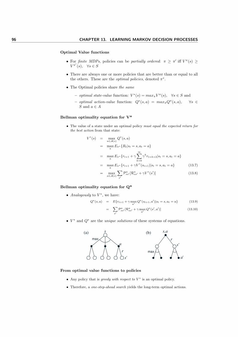
96 CHAPTER 13. LEARNING MARKOV DECISION PROCESSES
Optimal Value functions
• For finite MDPs, policies can be partially ordered: π ≥ π′ iff V π(s) ≥V π′(s), ∀s ∈ S
• There are always one or more policies that are better than or equal to allthe others. These are the optimal policies, denoted π∗.
• The Optimal policies share the same
– optimal state-value function: V ∗(s) = maxπVπ(s), ∀s ∈ S and
– optimal action-value function: Q∗(s, a) = maxπQπ(s, a), ∀s ∈
S and a ∈ A
Bellman optimality equation for V*
• The value of a state under an optimal policy must equal the expected return forthe best action from that state:
V ∗(s) = maxa∈A(s)
Q∗(s, a)
= maxa
Eπ∗{Rt|st = s, at = a}
= maxa
Eπ∗{rt+1 + γ
∞∑k=0
γkrt+k+2|st = s, at = a}
= maxa
Eπ∗{rt+1 + γV ∗(st+1)|st = s, at = a} (13.7)
= maxa∈A(s)
∑s′
Pass′ [Rass′ + γV ∗(s′)] (13.8)
Bellman optimality equation for Q*
• Analogously to V ∗, we have:
Q∗(s, a) = E{rt+1 + γmaxa′
Q∗(st+1, a′)|st = s, at = a} (13.9)
=∑s′Pass′ [R
ass′ + γmax
a′Q∗(s′, a′)] (13.10)
• V ∗ and Q∗ are the unique solutions of these systems of equations.
s,as
a
s'
r
a'
s'
r
(b)(a)
max
max
From optimal value functions to policies
• Any policy that is greedy with respect to V ∗ is an optimal policy.
• Therefore, a one-step-ahead search yields the long-term optimal actions.
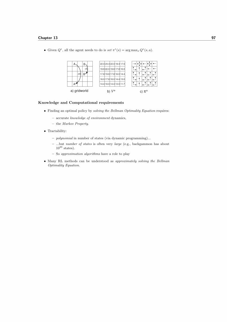
Chapter 13 97
• Given Q∗, all the agent needs to do is set π∗(s) = arg maxaQ∗(s, a).
a) gridworld b) V* c) π*
22.0 24.4 22.0 19.4 17.5
19.8 22.0 19.8 17.8 16.0
17.8 19.8 17.8 16.0 14.4
16.0 17.8 16.0 14.4 13.0
14.4 16.0 14.4 13.0 11.7
A B
A'
B'+10
+5
Knowledge and Computational requirements
• Finding an optimal policy by solving the Bellman Optimality Equation requires:
– accurate knowledge of environment dynamics,
– the Markov Property.
• Tractability:
– polynomial in number of states (via dynamic programming)...
– ...but number of states is often very large (e.g., backgammon has about1020 states).
– So approximation algorithms have a role to play
• Many RL methods can be understood as approximately solving the BellmanOptimality Equation.

14Solving MDPs: basic methods
The basic background & assumptions
• Environment is a finite MDP (i.e. A and S are finite).
• MDP’s dynamics defined by transition probabilities:
Pass′ = P (st+1 = s′|st = s, at = a)
• and expected immediate rewards,
Rass′ = E{rt+1|st = s, at = a, st+1 = s′}
• Goal: to search for good policies π
• Strategy: use value functions to structure search:
V ∗(s) = maxa
∑s′
Pass′ [Rass′ + γV ∗ (s′)] or
Q∗(s, a) =∑s′
Pass′ [Rass′ + γmaxa′
Q∗(s′, a′)]
Overview of methods for solving Bellman’s equations
• Dynamic programming:
– well-understood mathematical properties...
– ...but require a complete and accurate model of the environment
• Monte Carlo (simulation methods):
– conceptually simple
– no model required...
– ...but unsuitable for incremental computation
• Temporal difference methods
– also require no model;
– suitable for incremental computation...
– ... but mathematically complex to analyse
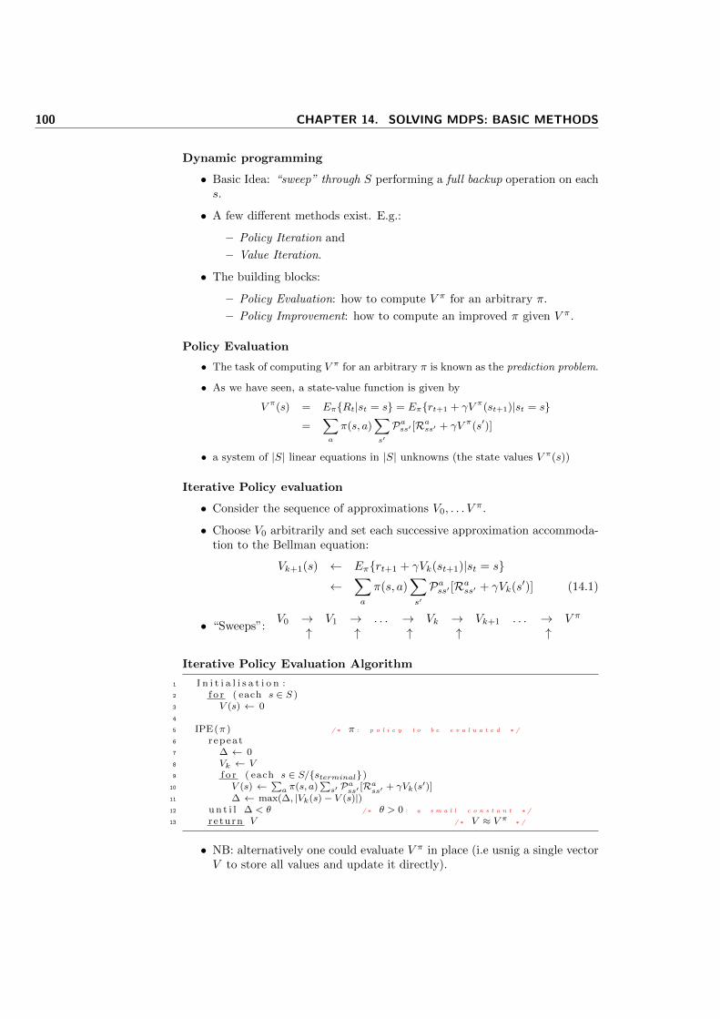
100 CHAPTER 14. SOLVING MDPS: BASIC METHODS
Dynamic programming
• Basic Idea: “sweep” through S performing a full backup operation on eachs.
• A few different methods exist. E.g.:
– Policy Iteration and
– Value Iteration.
• The building blocks:
– Policy Evaluation: how to compute V π for an arbitrary π.
– Policy Improvement: how to compute an improved π given V π.
Policy Evaluation
• The task of computing V π for an arbitrary π is known as the prediction problem.
• As we have seen, a state-value function is given by
V π(s) = Eπ{Rt|st = s} = Eπ{rt+1 + γV π(st+1)|st = s}
=∑a
π(s, a)∑s′
Pass′ [Rass′ + γV π(s′)]
• a system of |S| linear equations in |S| unknowns (the state values V π(s))
Iterative Policy evaluation
• Consider the sequence of approximations V0, . . . Vπ.
• Choose V0 arbitrarily and set each successive approximation accommoda-tion to the Bellman equation:
Vk+1(s) ← Eπ{rt+1 + γVk(st+1)|st = s}←
∑a
π(s, a)∑s′
Pass′ [Rass′ + γVk(s′)] (14.1)
• “Sweeps”:V0 → V1 → . . . → Vk → Vk+1 . . . → V π
↑ ↑ ↑ ↑ ↑
Iterative Policy Evaluation Algorithm
1 I n i t i a l i s a t i o n :2 f o r ( each s ∈ S )3 V (s) ← 04
5 IPE(π ) / ∗ π : p o l i c y t o b e e v a l u a t e d ∗ /
6 r epeat7 ∆ ← 08 Vk ← V9 f o r ( each s ∈ S/{sterminal})
10 V (s) ←∑a π(s, a)
∑s′ Pass′ [R
ass′ + γVk(s′)]
11 ∆ ← max(∆, |Vk(s)− V (s)|)12 u n t i l ∆ < θ / ∗ θ > 0 : a s m a l l c o n s t a n t ∗ /
13 r e turn V / ∗ V ≈ V π ∗ /
• NB: alternatively one could evaluate V π in place (i.e usnig a single vectorV to store all values and update it directly).
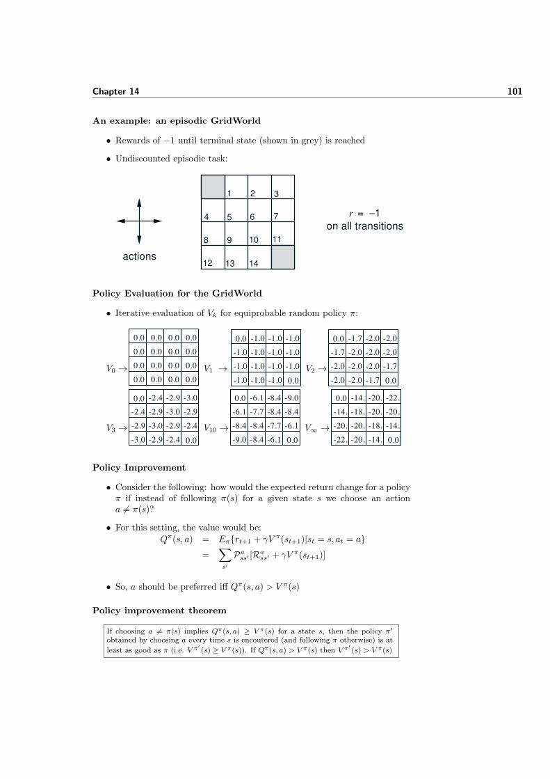
Chapter 14 101
An example: an episodic GridWorld
• Rewards of −1 until terminal state (shown in grey) is reached
• Undiscounted episodic task:
actions
r = −1
on all transitions
1 2 3
4 5 6 7
8 9 10 11
12 13 14
Policy Evaluation for the GridWorld
• Iterative evaluation of Vk for equiprobable random policy π:
V0 →
0.0 0.0 0.0
0.0 0.0 0.0 0.0
0.0 0.0 0.0 0.0
0.0 0.0 0.0
0.0
0.0
V1 →
-1.0 -1.0 -1.0
-1.0 -1.0 -1.0 -1.0
-1.0 -1.0 -1.0 -1.0
-1.0 -1.0 -1.0
0.0
0.0
V2 →
-1.7 -2.0 -2.0
-1.7 -2.0 -2.0 -2.0
-2.0 -2.0 -2.0 -1.7
-2.0 -2.0 -1.7
0.0
0.0
V3 →
-2.4 -2.9 -3.0
-2.4 -2.9 -3.0 -2.9
-2.9 -3.0 -2.9 -2.4
-3.0 -2.9 -2.4
0.0
0.0
V10 →
-6.1 -8.4 -9.0
-6.1 -7.7 -8.4 -8.4
-8.4 -8.4 -7.7 -6.1
-9.0 -8.4 -6.1
0.0
0.0
V∞ →
-14. -20. -22.
-14. -18. -20. -20.
-20. -20. -18. -14.
-22. -20. -14.
0.0
0.0
Policy Improvement
• Consider the following: how would the expected return change for a policyπ if instead of following π(s) for a given state s we choose an actiona 6= π(s)?
• For this setting, the value would be:
Qπ(s, a) = Eπ{rt+1 + γV π(st+1)|st = s, at = a}=
∑s′
Pass′ [Rass′ + γV π(st+1)]
• So, a should be preferred iff Qπ(s, a) > V π(s)
Policy improvement theorem
If choosing a 6= π(s) implies Qπ(s, a) ≥ V π(s) for a state s, then the policy π′
obtained by choosing a every time s is encoutered (and following π otherwise) is at
least as good as π (i.e. V π′(s) ≥ V π(s)). If Qπ(s, a) > V π(s) then V π
′(s) > V π(s)
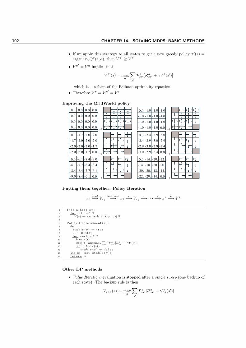
102 CHAPTER 14. SOLVING MDPS: BASIC METHODS
• If we apply this strategy to all states to get a new greedy policy π′(s) =arg maxaQ
π(s, a), then V π′ ≥ V π
• V π′ = V π implies that
V π′(s) = max
a
∑s′
Pass′ [Rass′ + γV π(s′)]
which is... a form of the Bellman optimality equation.
• Therefore V π = V π′
= V ∗
Improving the GridWorld policy
0.0 0.0 0.0
0.0 0.0 0.0 0.0
0.0 0.0 0.0 0.0
0.0 0.0 0.0
0.0
0.0 →
-1.0 -1.0 -1.0
-1.0 -1.0 -1.0 -1.0
-1.0 -1.0 -1.0 -1.0
-1.0 -1.0 -1.0
0.0
0.0 →-1.7 -2.0 -2.0
-1.7 -2.0 -2.0 -2.0
-2.0 -2.0 -2.0 -1.7
-2.0 -2.0 -1.7
0.0
0.0 →
-2.4 -2.9 -3.0
-2.4 -2.9 -3.0 -2.9
-2.9 -3.0 -2.9 -2.4
-3.0 -2.9 -2.4
0.0
0.0 →-6.1 -8.4 -9.0
-6.1 -7.7 -8.4 -8.4
-8.4 -8.4 -7.7 -6.1
-9.0 -8.4 -6.1
0.0
0.0 →
-14. -20. -22.
-14. -18. -20. -20.
-20. -20. -18. -14.
-22. -20. -14.
0.0
0.0 →
Putting them together: Policy Iteration
π0eval−→ Vπ0
improve−→ π1e−→ Vπ1
i−→ · · · i−→ π∗e−→ V ∗
1 I n i t i a l i s a t i o n :2 f o r a l l s ∈ S3 V (s) ← an a r b i t r a r y v ∈ R4
5 Policy Improvement (π ) :6 do7 s t a b l e (π ) ← t rue8 V ← IPE(π )9 f o r each s ∈ S
10 b ← π(s)11 π(s) ← arg maxa
∑s′ P
ass′ [R
ass′ + γV (s′)]
12 i f ( b 6= π(s))13 s t a b l e (π ) ← f a l s e14 whi le ( not s t a b l e (π ) )15 re turn π
Other DP methods
• Value Iteration: evaluation is stopped after a single sweep (one backup ofeach state). The backup rule is then:
Vk+1(s)← maxa
∑s′
Pass′ [Rass′ + γVk(s′)]
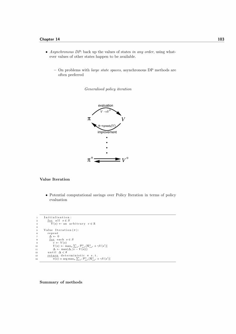
Chapter 14 103
• Asynchronous DP: back up the values of states in any order, using what-ever values of other states happen to be available.
– On problems with large state spaces, asynchronous DP methods areoften preferred
Generalised policy iteration
Value Iteration
• Potential computational savings over Policy Iteration in terms of policyevaluation
1 I n i t i a l i s a t i o n :2 f o r a l l s ∈ S3 V (s) ← an a r b i t r a r y v ∈ R4
5 Value I t e r a t i o n (π ) :6 repeat7 ∆ ← 08 f o r each s ∈ S9 v ← V (s)
10 V (s) ← maxa∑s′ P
ass′ [R
ass′ + γV (s′)]
11 ∆ ← max(∆, |v − V (s)|)12 u n t i l ∆ < θ13 re turn d e t e r m i n i s t i c π s . t .14 π(s) = arg maxa
∑s′ P
ass′ [R
ass′ + γV (s′)]
Summary of methods
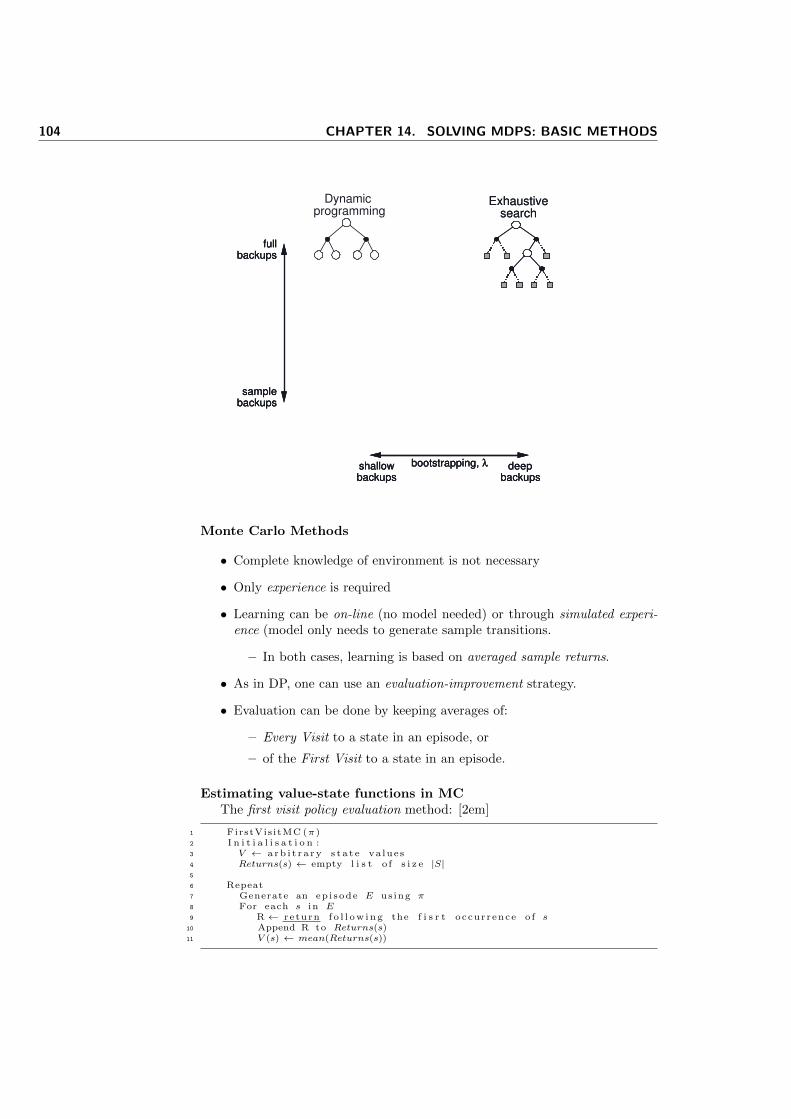
104 CHAPTER 14. SOLVING MDPS: BASIC METHODS
bootstrapping, λ
fullbackups
samplebackups
shallowbackups
deepbackups
bootstrapping, λ
fullbackups
samplebackups
shallowbackups
deepbackups
Exhaustivesearch
bootstrapping, λ
fullbackups
samplebackups
shallowbackups
deepbackups
Exhaustivesearch
Dynamicprogramming
Monte Carlo Methods
• Complete knowledge of environment is not necessary
• Only experience is required
• Learning can be on-line (no model needed) or through simulated experi-ence (model only needs to generate sample transitions.
– In both cases, learning is based on averaged sample returns.
• As in DP, one can use an evaluation-improvement strategy.
• Evaluation can be done by keeping averages of:
– Every Visit to a state in an episode, or
– of the First Visit to a state in an episode.
Estimating value-state functions in MCThe first visit policy evaluation method: [2em]
1 FirstVis itMC (π )2 I n i t i a l i s a t i o n :3 V ← a r b i t r a r y s t a t e va lues4 Returns(s) ← empty l i s t o f s i z e |S|5
6 Repeat7 Generate an ep i sode E us ing π8 For each s in E9 R ← re turn f o l l o w i n g the f i s r t occurrence o f s
10 Append R to Returns(s)11 V (s) ← mean(Returns(s))
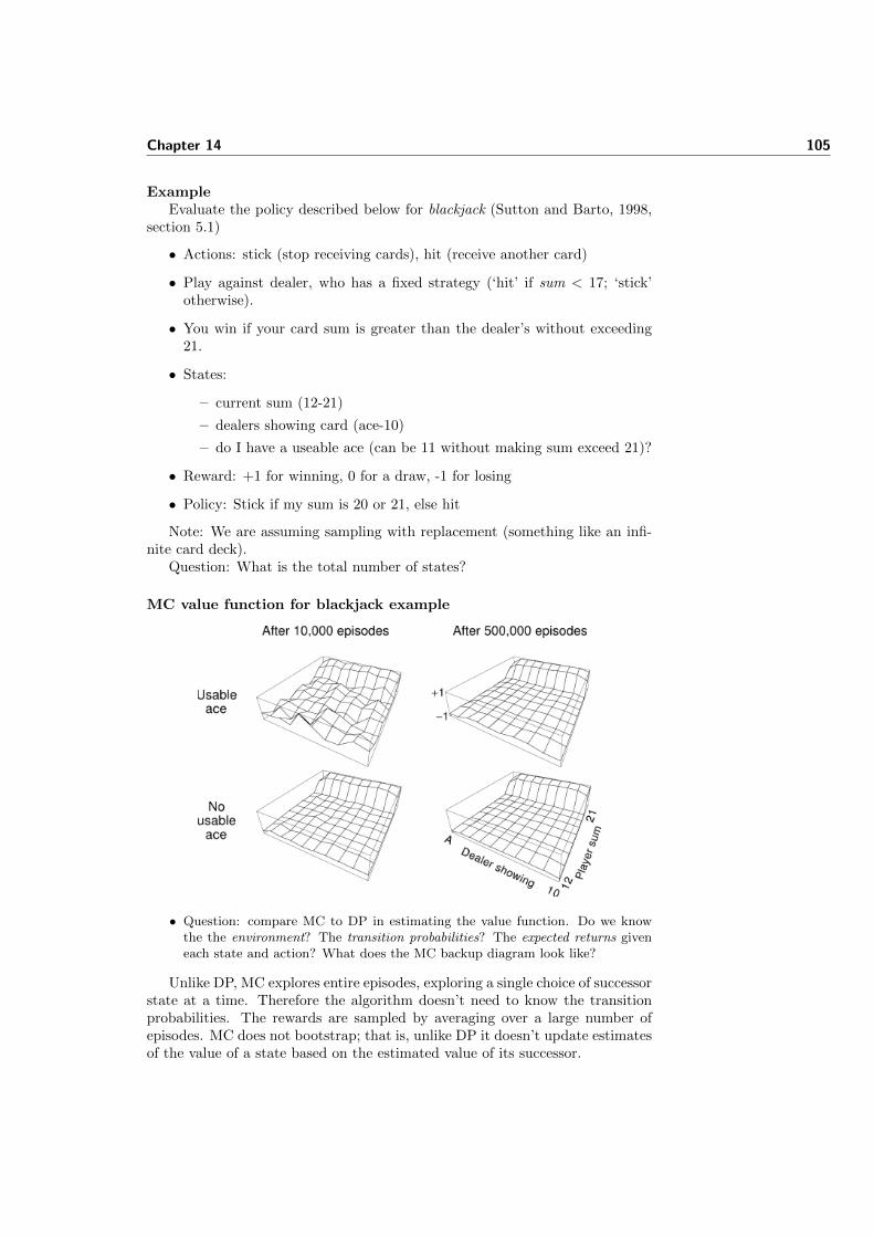
Chapter 14 105
ExampleEvaluate the policy described below for blackjack (Sutton and Barto, 1998,
section 5.1)
• Actions: stick (stop receiving cards), hit (receive another card)
• Play against dealer, who has a fixed strategy (‘hit’ if sum < 17; ‘stick’otherwise).
• You win if your card sum is greater than the dealer’s without exceeding21.
• States:
– current sum (12-21)
– dealers showing card (ace-10)
– do I have a useable ace (can be 11 without making sum exceed 21)?
• Reward: +1 for winning, 0 for a draw, -1 for losing
• Policy: Stick if my sum is 20 or 21, else hit
Note: We are assuming sampling with replacement (something like an infi-nite card deck).
Question: What is the total number of states?
MC value function for blackjack example
• Question: compare MC to DP in estimating the value function. Do we knowthe the environment? The transition probabilities? The expected returns giveneach state and action? What does the MC backup diagram look like?
Unlike DP, MC explores entire episodes, exploring a single choice of successorstate at a time. Therefore the algorithm doesn’t need to know the transitionprobabilities. The rewards are sampled by averaging over a large number ofepisodes. MC does not bootstrap; that is, unlike DP it doesn’t update estimatesof the value of a state based on the estimated value of its successor.
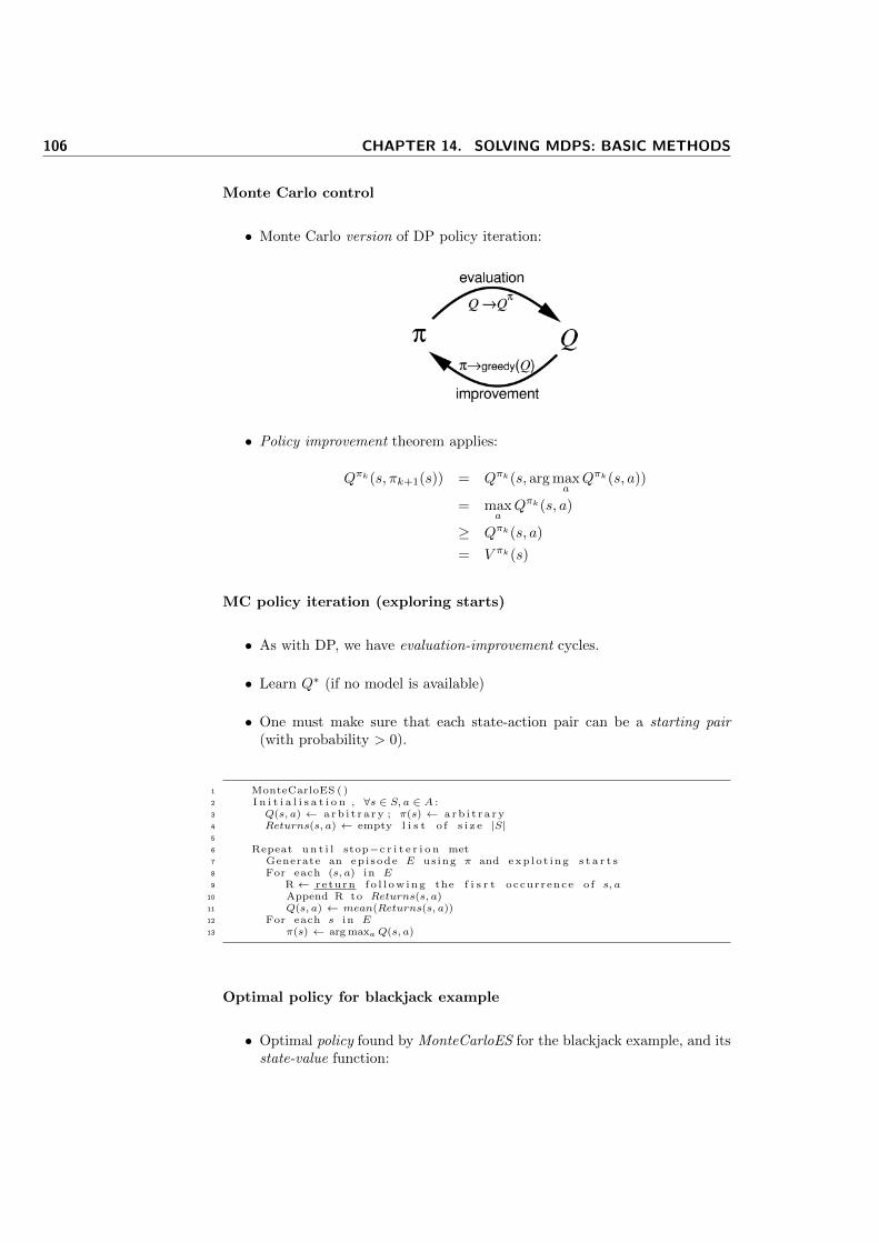
106 CHAPTER 14. SOLVING MDPS: BASIC METHODS
Monte Carlo control
• Monte Carlo version of DP policy iteration:
• Policy improvement theorem applies:
Qπk(s, πk+1(s)) = Qπk(s, arg maxa
Qπk(s, a))
= maxa
Qπk(s, a)
≥ Qπk(s, a)
= V πk(s)
MC policy iteration (exploring starts)
• As with DP, we have evaluation-improvement cycles.
• Learn Q∗ (if no model is available)
• One must make sure that each state-action pair can be a starting pair(with probability > 0).
1 MonteCarloES ( )2 I n i t i a l i s a t i o n , ∀s ∈ S, a ∈ A :3 Q(s, a) ← a r b i t r a r y ; π(s) ← a r b i t r a r y4 Returns(s, a) ← empty l i s t o f s i z e |S|5
6 Repeat u n t i l stop−c r i t e r i o n met7 Generate an ep i sode E us ing π and exp lo t ing s t a r t s8 For each (s, a) in E9 R ← re turn f o l l o w i n g the f i s r t occurrence o f s, a
10 Append R to Returns(s, a)11 Q(s, a) ← mean(Returns(s, a))12 For each s in E13 π(s) ← arg maxaQ(s, a)
Optimal policy for blackjack example
• Optimal policy found by MonteCarloES for the blackjack example, and itsstate-value function:
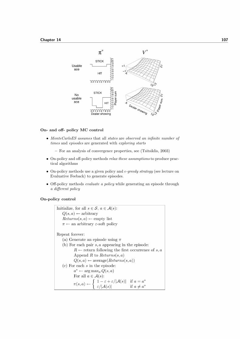
Chapter 14 107
On- and off- policy MC control
• MonteCarloES assumes that all states are observed an infinite number oftimes and episodes are generated with exploring starts
– For an analysis of convergence properties, see (Tsitsiklis, 2003)
• On-policy and off-policy methods relax these assumptions to produce prac-tical algorithms
• On-policy methods use a given policy and ε-greedy strategy (see lecture onEvaluative Feeback) to generate episodes.
• Off-policy methods evaluate a policy while generating an episode througha different policy
On-policy control
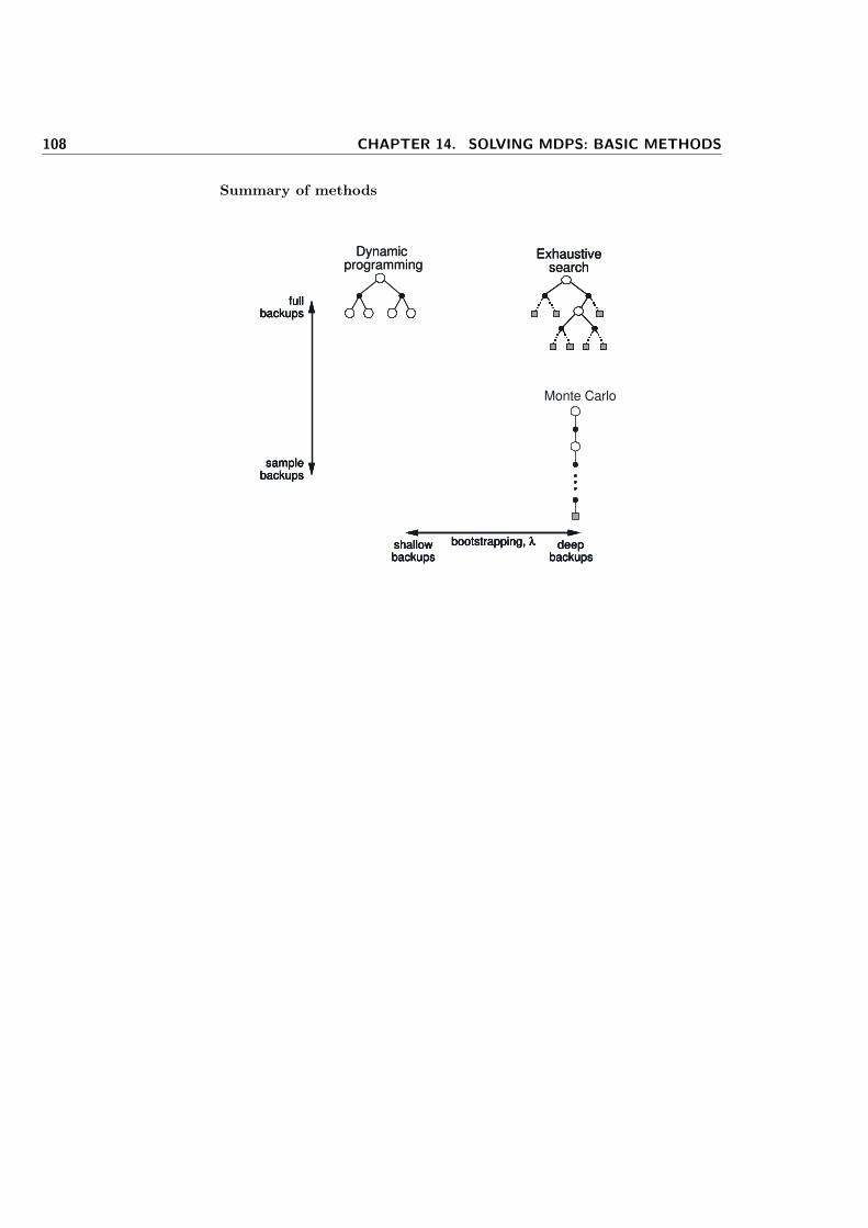
108 CHAPTER 14. SOLVING MDPS: BASIC METHODS
Summary of methods
bootstrapping, λ
fullbackups
samplebackups
shallowbackups
deepbackups
bootstrapping, λ
fullbackups
samplebackups
shallowbackups
deepbackups
Exhaustivesearch
bootstrapping, λ
fullbackups
samplebackups
shallowbackups
deepbackups
Exhaustivesearch
Dynamicprogramming
bootstrapping, λ
fullbackups
samplebackups
shallowbackups
deepbackups
Exhaustivesearch
Dynamicprogramming
Monte Carlo
15Temporal Difference Learning
Recall background & assumptions
• Environment is a finite MDP (i.e. A and S are finite).
• MDP’s dynamics defined by transition probabilities:
Pass′ = P (st+1 = s′|st = s, at = a)
• and expected immediate rewards,
Rass′ = E{rt+1|st = s, at = a, st+1 = s′}
• Goal: to search for good policies π
• DP Strategy: use value functions to structure search:
V ∗(s) = maxa
∑s′
Pass′ [Rass′ + γV ∗(s′)] or
Q∗(s, a) =∑s′
Pass′ [Rass′ + γmaxa′
Q∗(s′, a′)]
• MC strategy: expand each episode and keep averages of returns per state.
Temporal Difference (TD) Learning
• TD is a combination of ideas from Monte Carlo methods and DP methods:
– TD can learn directly from raw experience without a model of theenvironment’s dynamics, like MC.
– TD methods update estimates based in part on other learned esti-mates, without waiting for a final outcome (i.e. they “bootstrap”),like DP
• Some widely used TD methods: TD(0), TD(λ), Sarsa, Q-learning, Actor-critic, R-Learning
110 CHAPTER 15. TEMPORAL DIFFERENCE LEARNING
Prediction & Control
• Recall value function estimation (prediction) for DP and MC:
– Updates for DP:
V π(s) = Eπ{Rt|st = s}= Eπ{rt+1 + γV π(st+1)|st = s}
– Update rule for MC:
V (st)← V (st) + α[Rt − γV (st)]
(Q: why are the value functions above merely estimates?)
Prediction in TD(0)
• Prediction (update of estimates of V ) for the TD(0) method is done asfollows:
V (st)← V (st) + α[ rt+1 + γV (st+1)︸ ︷︷ ︸1-step estimate of Rt
−V (st)] (15.1)
• No need to wait until the end of the episode (as in MC) to update V
• No need to sweep across the possible successor states (as in DP).
Tabular TD(0) value function estimation
• Use sample backup (as in MC) rather than full backup (as in DP):
Algorithm 15.1: TD(0)
1 TabularTD0 (π )2 I n i t i a l i s a t i o n , ∀s ∈ S :3 V (s) ← a r b i t r a r y ;4 α ← l e a r n i n g constant5 γ ← di scount f a c t o r6
7 For each ep i sode E u n t i l stop−c r i t e r i o n met8 I n i t i a l i s e s9 For each step o f E
10 a ← π(s)11 Take ac t i on a ;12 Observe reward r and next s t a t e s′
13 V (s) ← V (s) + α[r + γV (s′)− V (s)]14 s ← s′
15 u n t i l s i s a te rmina l s t a t e
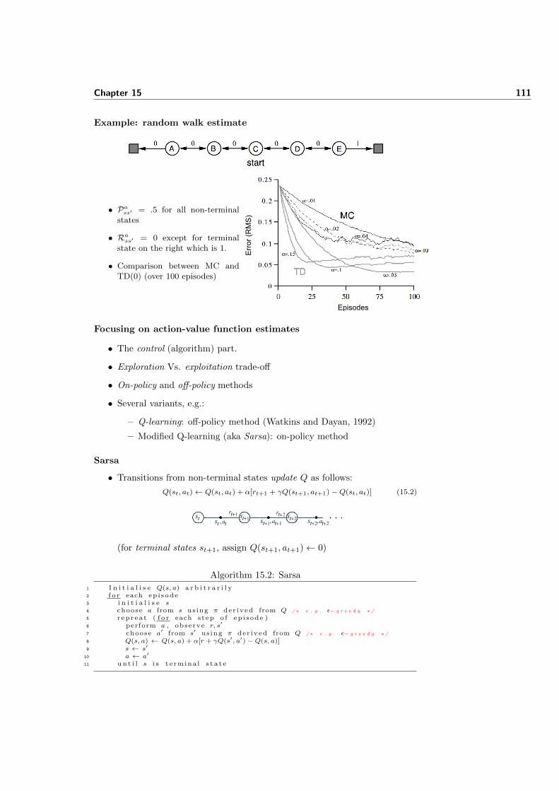
Chapter 15 111
Example: random walk estimate
• Pass′ = .5 for all non-terminalstates
• Rass′ = 0 except for terminalstate on the right which is 1.
• Comparison between MC andTD(0) (over 100 episodes)
Err
or (
RM
S)
Episodes
Focusing on action-value function estimates
• The control (algorithm) part.
• Exploration Vs. exploitation trade-off
• On-policy and off-policy methods
• Several variants, e.g.:
– Q-learning: off-policy method (Watkins and Dayan, 1992)
– Modified Q-learning (aka Sarsa): on-policy method
Sarsa
• Transitions from non-terminal states update Q as follows:
Q(st, at)← Q(st, at) + α[rt+1 + γQ(st+1, at+1)−Q(st, at)] (15.2)
st+2
,at+2
st+1
,at+1
rt+2
rt+1
st
st+1
st ,a
t
st+2
(for terminal states st+1, assign Q(st+1, at+1)← 0)
Algorithm 15.2: Sarsa
1 I n i t i a l i s e Q(s, a) a r b i t r a r i l y2 f o r each ep i sode3 i n i t i a l i s e s4 choose a from s us ing π der ived from Q /∗ e . g . ε− g r e e d y ∗ /5 r ep r ea t ( f o r each step o f ep i sode )6 perform a , observe r, s′
7 choose a′ from s′ us ing π der ived from Q /∗ e . g . ε− g r e e d y ∗ /8 Q(s, a) ← Q(s, a) + α[r + γQ(s′, a′)−Q(s, a)]9 s ← s′
10 a ← a′
11 u n t i l s i s t e rmina l s t a t e
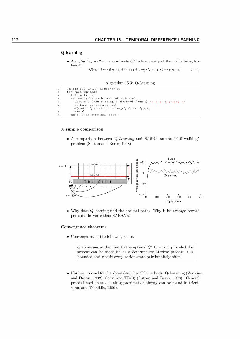
112 CHAPTER 15. TEMPORAL DIFFERENCE LEARNING
Q-learning
• An off-policy method: approximate Q∗ independently of the policy being fol-lowed:
Q(st, at)← Q(st, at) + α[rt+1 + γmaxa
Q(st+1, a)−Q(st, at)] (15.3)
Algorithm 15.3: Q-Learning
1 I n i t i a l i s e Q(s, a) a r b i t r a r i l y2 f o r each ep i sode3 i n i t i a l i s e s4 r ep r ea t ( f o r each step o f ep i sode )5 choose a from s us ing π der ived from Q /∗ e . g . ε− g r e e d y ∗ /6 perform a , observe r, s′
7 Q(s, a) ← Q(s, a) + α[r + γmaxa′ Q(s′, a′)−Q(s, a)]8 s ← s′
9 u n t i l s i s t e rmina l s t a t e
A simple comparison
• A comparison between Q-Learning and SARSA on the “cliff walking”problem (Sutton and Barto, 1998)
Safe Path
Optimal Path
Ave
rage
rew
ard
per
ep
isod
e
• Why does Q-learning find the optimal path? Why is its average rewardper episode worse than SARSA’s?
Convergence theorems
• Convergence, in the following sense:
Q converges in the limit to the optimal Q∗ function, provided thesystem can be modelled as a deterministc Markov process, r isbounded and π visit every action-state pair infinitely often.
• Has been proved for the above described TD methods: Q-Learning (Watkinsand Dayan, 1992), Sarsa and TD(0) (Sutton and Barto, 1998). Generalproofs based on stochastic approximation theory can be found in (Bert-sekas and Tsitsiklis, 1996).
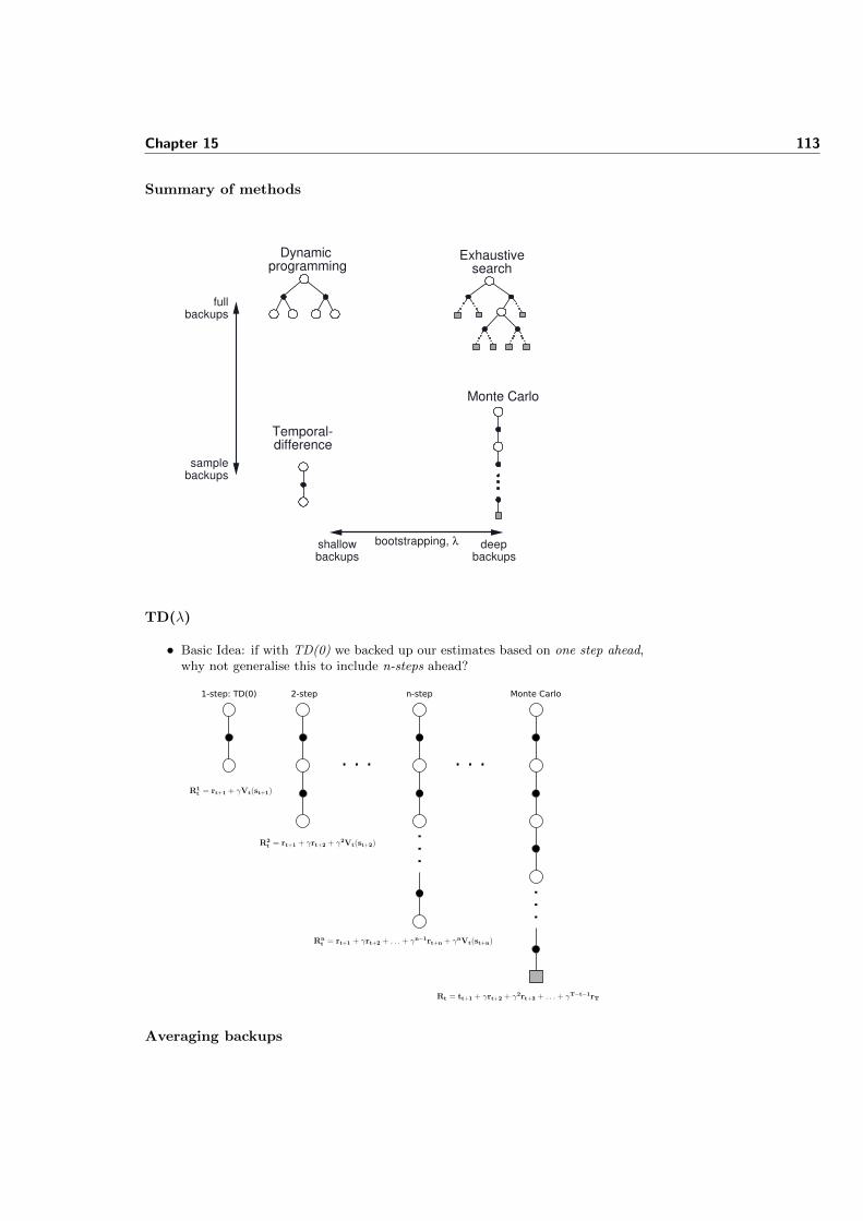
Chapter 15 113
Summary of methods
bootstrapping, λ
fullbackups
samplebackups
shallowbackups
deepbackups
Exhaustivesearch
Dynamicprogramming
Monte Carlo
Temporal-difference
TD(λ)
• Basic Idea: if with TD(0) we backed up our estimates based on one step ahead,why not generalise this to include n-steps ahead?
. . . . . .
2-step1-step: TD(0)
. . .
n-step
. . .
Monte Carlo
Averaging backups
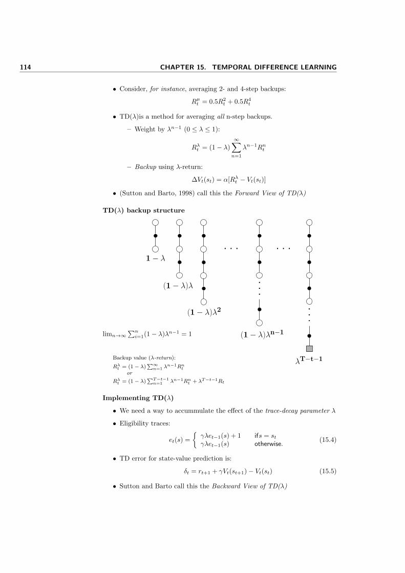
114 CHAPTER 15. TEMPORAL DIFFERENCE LEARNING
• Consider, for instance, averaging 2- and 4-step backups:
Rµt = 0.5R2t + 0.5R4
t
• TD(λ)is a method for averaging all n-step backups.
– Weight by λn−1 (0 ≤ λ ≤ 1):
Rλt = (1− λ)
∞∑n=1
λn−1Rnt
– Backup using λ-return:
∆Vt(st) = α[Rλt − Vt(st)]
• (Sutton and Barto, 1998) call this the Forward View of TD(λ)
TD(λ) backup structure
. . . . . .
. . .
. . .
limn→∞∑ni=1(1− λ)λn−1 = 1
Backup value (λ-return):
Rλt = (1− λ)∑∞n=1 λ
n−1Rntor
Rλt = (1− λ)∑T−t−1n=1 λn−1Rnt + λT−t−1Rt
Implementing TD(λ)
• We need a way to accummulate the effect of the trace-decay parameter λ
• Eligibility traces:
et(s) =
{γλet−1(s) + 1 ifs = stγλet−1(s) otherwise.
(15.4)
• TD error for state-value prediction is:
δt = rt+1 + γVt(st+1)− Vt(st) (15.5)
• Sutton and Barto call this the Backward View of TD(λ)
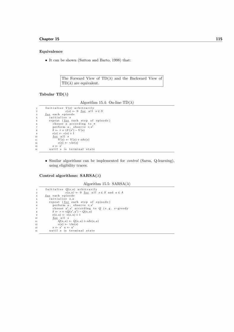
Chapter 15 115
Equivalence
• It can be shown (Sutton and Barto, 1998) that:
The Forward View of TD(λ) and the Backward View ofTD(λ) are equivalent.
Tabular TD(λ)
Algorithm 15.4: On-line TD(λ)
1 I n i t i a l i s e V (s) a r b i t r a r i l y2 e(s) ← 0 f o r a l l s ∈ S3 f o r each ep i sode4 i n i t i a l i s e s5 repeat ( f o r each step o f ep i sode )6 choose a accord ing to π7 perform a , observe r, s′
8 δ ← r + γV (s′)− V (s)9 e(s) ← e(s) + 1
10 f o r a l l s11 V (s) ← V (s) + αδe(s)12 e(s) ← γλe(s)13 s ← s′
14 u n t i l s i s t e rmina l s t a t e
• Similar algorithms can be implemented for control (Sarsa, Q-learning),using eligibility traces.
Control algorithms: SARSA(λ)
Algorithm 15.5: SARSA(λ)
1 I n i t i a l i s e Q(s, a) a r b i t r a r i l y2 e(s, a) ← 0 f o r a l l s ∈ S and a ∈ A3 f o r each ep i sode4 i n i t i a l i s e s, a5 repeat ( f o r each step o f ep i sode )6 perform a , observe r, s′
7 choose a′, s′ accord ing to Q ( e . g . ε−greedy8 δ ← r + γQ(s′, a′)−Q(s, a)9 e(s, a) ← e(s, a) + 1
10 f o r a l l s11 Q(s, a) ← Q(s, a) + αδe(s, a)12 e(s) ← γλe(s)13 s ← s′ a ← a′
14 u n t i l s i s t e rmina l s t a t e

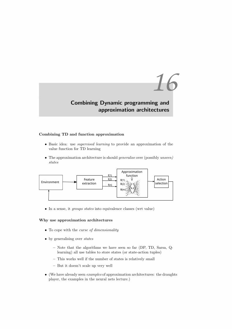
16Combining Dynamic programming and
approximation architectures
Combining TD and function approximation
• Basic idea: use supervised learning to provide an approximation of thevalue function for TD learning
• The approximation architecture is should generalise over (possibly unseen)states
EnvironmentFeature
extraction
Approximation function
V~ Actionselection
θ(1)
θ(2)
θ(m)
.
.
.
f(1)
f(2)
f(n)...
• In a sense, it groups states into equivalence classes (wrt value)
Why use approximation architectures
• To cope with the curse of dimensionality
• by generalising over states
– Note that the algorithms we have seen so far (DP, TD, Sarsa, Q-learning) all use tables to store states (or state-action tuples)
– This works well if the number of states is relatively small
– But it doesn’t scale up very well
• (We have already seen examples of approximation architectures: the draughtsplayer, the examples in the neural nets lecture.)
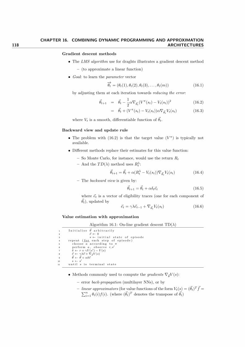
118CHAPTER 16. COMBINING DYNAMIC PROGRAMMING AND APPROXIMATION
ARCHITECTURES
Gradient descent methods
• The LMS algorithm use for draghts illustrates a gradient descent method
– (to approximate a linear function)
• Goal: to learn the parameter vector
−→θt = (θt(1), θt(2), θt(3), . . . , θt(m)) (16.1)
by adjusting them at each iteration towards reducing the error:
~θt+1 = ~θt −1
2α∇~θt(V
π(st)− Vt(st))2 (16.2)
= ~θt + (V π(st)− Vt(st))α∇~θtVt(st) (16.3)
where Vt is a smooth, differentiable function of ~θt.
Backward view and update rule
• The problem with (16.2) is that the target value (V π) is typically notavailable.
• Different methods replace their estimates for this value function:
– So Monte Carlo, for instance, would use the return Rt
– And the TD(λ) method uses Rλt :
~θt+1 = ~θt + α(Rλt − Vt(st))∇~θtVt(st) (16.4)
– The backward view is given by:
~θt+1 = ~θt + αδt~et (16.5)
where ~et is a vector of eligibility traces (one for each component of~θt), updated by
~et = γλ~et−1 +∇~θtVt(st) (16.6)
Value estimation with approximation
Algorithm 16.1: On-line gradient descent TD(λ)
1 I n i t i a l i s e ~θ a r b i t r a r i l y2 ~e ← 03 s ← i n i t i a l s t a t e o f ep i sode4 repeat ( f o r each step o f ep i sode )5 choose a accord ing to π6 perform a , observe r, s′
7 δ ← r + γV (s′)− V (s)8 ~e ← γλ~e+∇~θV (s)
9 ~θ ← ~θ + αδ~e10 s ← s′
11 u n t i l s i s t e rmina l s t a t e
• Methods commonly used to compute the gradients ∇~θV (s):
– error back-propagation (multilayer NNs), or by
– linear approximators (for value functions of the form Vt(s) = (~θt)T ~f =∑n
i=1 θt(i)f(i). (where (~θt)T denotes the transpose of ~θt)
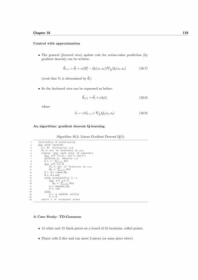
Chapter 16 119
Control with approximation
• The general (forward view) update rule for action-value prediction (bygradient descent) can be written:
~θt+1 = ~θt + α(Rλt −Qt(st, at))∇~θtQt(st, at) (16.7)
(recal that Vt is determined by ~θt)
• So the backward view can be expressed as before:
~θt+1 = ~θt + αδt~et (16.8)
where
~et = γλ~et−1 +∇~θtQt(st, at) (16.9)
An algorithm: gradient descent Q-learning
Algorithm 16.2: Linear Gradient Descent Q(λ)
1 I n i t i a l i s e θ a r b i t r a r i l y2 f o r each ep i sode
3 ~e ← ~0 ; i n i t i a l i s e s, a4 Fa ← s e t o f f e a t u r e s in s, a5 repeat ( f o r each step o f ep i sode )6 f o r a l l i ∈ Fa : e(i) ← e(i) + 17 perform a , observe r, s8 δ ← r −
∑i∈Fa θ(i)
9 f o r a l l a ∈ A10 Fa ← s e t o f f e a t u r e s in s, a11 Qa ←
∑i∈Fa θ(i)
12 δ ← δ + γmaxaQa13 ~θ ← ~θ + αδ~e14 with p r o b a b i l i t y 1− ε15 f o r a l l a ∈ A16 Qa ←
∑i∈Fa θ(i)
17 a ← arg maxaQa18 ~e ← γλ~e19 e l s e20 a ← a random act i on21 ~e ← 022 u n t i l s i s t e rmina l s t a t e
A Case Study: TD-Gammon
• 15 white and 15 black pieces on a board of 24 locations, called points.
• Player rolls 2 dice and can move 2 pieces (or same piece twice)
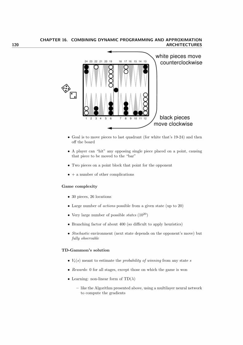
120CHAPTER 16. COMBINING DYNAMIC PROGRAMMING AND APPROXIMATION
ARCHITECTURES
• Goal is to move pieces to last quadrant (for white that’s 19-24) and thenoff the board
• A player can “hit” any opposing single piece placed on a point, causingthat piece to be moved to the “bar”
• Two pieces on a point block that point for the opponent
• + a number of other complications
Game complexity
• 30 pieces, 26 locations
• Large number of actions possible from a given state (up to 20)
• Very large number of possible states (1020)
• Branching factor of about 400 (so difficult to apply heuristics)
• Stochastic environment (next state depends on the opponent’s move) butfully observable
TD-Gammon’s solution
• Vt(s) meant to estimate the probability of winning from any state s
• Rewards: 0 for all stages, except those on which the game is won
• Learning: non-linear form of TD(λ)
– like the Algorithm presented above, using a multilayer neural networkto compute the gradients
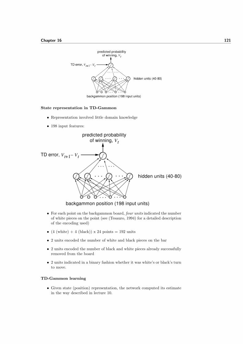
Chapter 16 121
State representation in TD-Gammon
• Representation involved little domain knowledge
• 198 input features:
• For each point on the backgammon board, four units indicated the numberof white pieces on the point (see (Tesauro, 1994) for a detailed descriptionof the encoding used)
• (4 (white) + 4 (black)) x 24 points = 192 units
• 2 units encoded the number of white and black pieces on the bar
• 2 units encoded the number of black and white pieces already successfullyremoved from the board
• 2 units indicated in a binary fashion whether it was white’s or black’s turnto move.
TD-Gammon learning
• Given state (position) representation, the network computed its estimatein the way described in lecture 10.
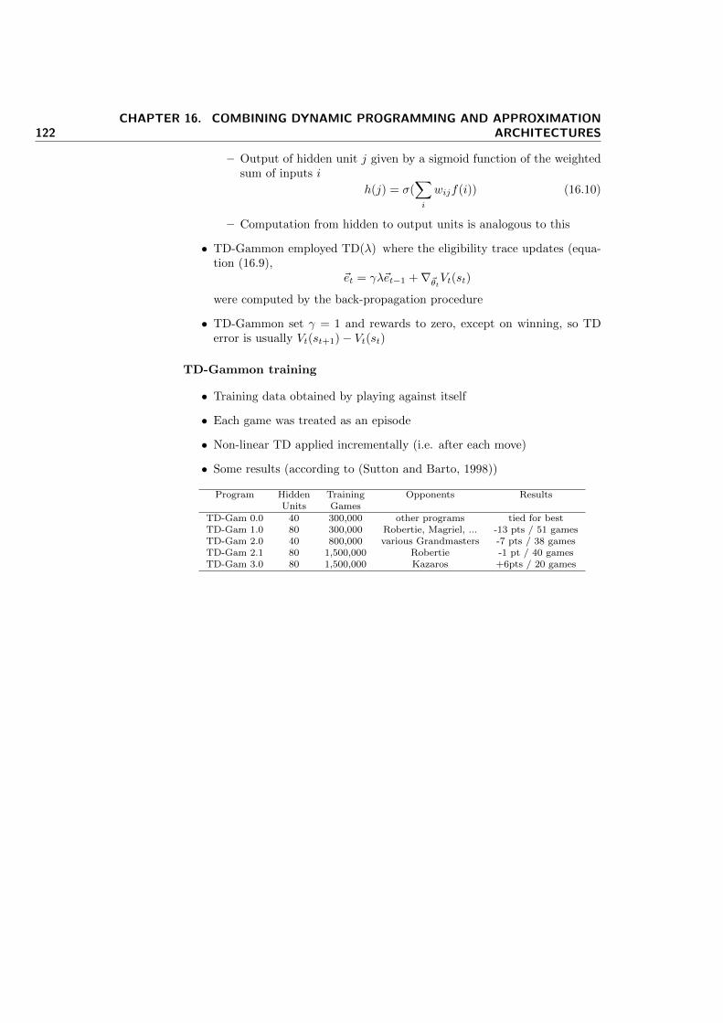
122CHAPTER 16. COMBINING DYNAMIC PROGRAMMING AND APPROXIMATION
ARCHITECTURES
– Output of hidden unit j given by a sigmoid function of the weightedsum of inputs i
h(j) = σ(∑i
wijf(i)) (16.10)
– Computation from hidden to output units is analogous to this
• TD-Gammon employed TD(λ) where the eligibility trace updates (equa-tion (16.9),
~et = γλ~et−1 +∇~θtVt(st)were computed by the back-propagation procedure
• TD-Gammon set γ = 1 and rewards to zero, except on winning, so TDerror is usually Vt(st+1)− Vt(st)
TD-Gammon training
• Training data obtained by playing against itself
• Each game was treated as an episode
• Non-linear TD applied incrementally (i.e. after each move)
• Some results (according to (Sutton and Barto, 1998))
Program Hidden Training Opponents ResultsUnits Games
TD-Gam 0.0 40 300,000 other programs tied for bestTD-Gam 1.0 80 300,000 Robertie, Magriel, ... -13 pts / 51 gamesTD-Gam 2.0 40 800,000 various Grandmasters -7 pts / 38 gamesTD-Gam 2.1 80 1,500,000 Robertie -1 pt / 40 gamesTD-Gam 3.0 80 1,500,000 Kazaros +6pts / 20 games
17Final Project
17.1 Background
This end-of-course project will account for 70% of your overall grade in CS7032.The project can be done individually or in teams of two students.
The project will be assessed through a report and code. In some cases, ademonstration might also be appropriate and will be arranged in advance. Thereport must be structured as an academic paper and contain, minimally: (1)a precise statement of the problem addressed by the project, (2) the approachyou adopted to solving it, (3) a discussion of you results (whether positive ornegative), (4) the main difficulties you encountered, (5) your assessment of theusefulness of an AI technique in addressing the type of problem tackled by yourproject and (6) references to the relevant literature. In addition, if you workedas a team, you must include a separate section describing the contribution ofeach team member.
17.2 Goals
You should implement an agent (or controller for a team of agents, as the casemight be) to play one of the recommended Game AI competitions. Althoughwe should ultimately be aiming to produce an agent (or agents) which canin principle (say, after some extra work after the assignment itself is finished)be entered into a competition, some competitions may be too complex for acomplete and competitive agent to be implemented within the time frame ofthe project. In such cases, it is acceptable for you to focus on an interestingaspect or sub-problem of the game in question (e.g. learning targeting or movestrategies in combat-style games, learning the best choice of shooting techniquein Angry Birds (e.g. (Jutzeler et al., 2013)), learning defense actions in fightinggames (e.g. (Yamamoto et al., 2014)), etc).
124 CHAPTER 17. FINAL PROJECT
17.3 Assessment
The project will be assessed and marked in terms of: (a) clarity of problem de-scription, including adequate (not excessive) background information, (b) qual-ity of the technical execution, bearing in mind that we are not looking foran unbeatable agent but one that illustrates clearly and meaningfully some ofthe techniques discussed in the course (such as problem specification in terms ofagent architectures, simulation and multi-agent problem solving, supervised andreinforcement learning, etc), (c) clarity in the assessment of results, discussionof the effectiveness of the techniques explored, and conclusions drawn from theproject work, (d) quality of the presentation and (e) description and assessmentof the contributions of each team member (if you choose to work in a team).
The amount of effort you should put into the project should be commensu-rable with the amount of work put into preparing for an exam.
17.4 Delivering the assignment
The deadline for submission of the project report (and code) is Monday, 26thJanuary. The project must be submitted through blackboard, as with the otherassignments.
Please format the report (preferably in LATEX) according to the ACM’s con-ference proceedings style template1. The report/paper should normally notexceed 10 pages in the (two column) ACM format.
17.5 Possible choices
You may choose one of the following competitions:
1. Fighting AI,
2. AI Birds,
3. Starcraft or
4. Vindinium
These options are recommended based on the following criteria: your ex-pressed preferences, availability (and freedom) of code, interest of the AI com-munity in general (as reflected in published papers and competitions scheduledfor next year’s AI conferences), simplicity of the domain (so that you can focuson the AI).
17.5.1 Resources
Surveys and links to the competitions, papers etc can be found at the coursewebsite2.
1http://www.acm.org/sigs/publications/proceedings-templates#aL12https://www.scss.tcd.ie/~luzs/t/cs7032/gamesaisurvey-teams.html

Chapter 17 125
17.6 Questions?
Feel free to email me.

Bibliography
Bellman, R. (1956). A problem in the sequential design of experiments. Sankhya,16:221–229.
Berger, B. and Leighton, T. (1998). Protein folding in the hydrophobic-hydrophilic (hp) is np-complete. In Proceedings of the second annual in-ternational conference on Computational molecular biology, pages 30–39.ACM Press.
Bertsekas, D. P. and Tsitsiklis, J. N. (1996). Neuro-Dynamic Programming.Athena Scientific, Belmont.
Bonabeau, E., Dorigo, M., and Theraulaz, G. (2000). Inspiration for optimiza-tion from social insect behaviour. Nature, 4006.
Brooks, R. A. (1986). A robust layered control system for a mobile robot. IEEEJournal of Robotics and Automation, RA-2(1):14–23.
Caro, G. D. and Dorigo, M. (1998). Antnet: Distributed stigmergetic controlfor communications networks. Journal of Artificial Intelligence Research,9:317–365.
Cassell, J. (2000). Embodied conversational interface agents. Communicationsof the ACM, 43(4):70–78.
Chapman, D. and Agre, P. E. (1987). Pengi: An implementation of a theoryof activity. Technical report, Massachusetts Institute of Technology, A.I.Lab., Cambridge, Massachusetts. Subm. to the Cognitive Modeling/ScienceSection of AAAI-87.
Crescenzi, P., Goldman, D., Papadimitriou, C., Piccolboni, A., and Yannakakis,M. (1998). On the complexity of protein folding (abstract). In Proceedingsof the second annual international conference on Computational molecularbiology, pages 61–62. ACM Press.
128 Bibliography
Dill, K. A., Bromberg, S., Yue, K., Fiebig, K. M., Yee, D. P., Thomas, P. D.,and Chan, H. S. (1995). Principles of protein folding – A perspective fromsimple exact models. Protein Science, 4(4):561–602.
Domingos, P. (2012). A few useful things to know about machine learning.Communications of the ACM, 55(10):78–87.
Dorigo, M. and Di Caro, G. (1999). The ant colony optimization meta-heuristic.In Corne, D., Dorigo, M., and Glover, F., editors, New Ideas in Optimiza-tion, pages 11–32. McGraw-Hill, London.
Dorigo, M., Maniezzo, V., and Colorni, A. (1996). The Ant System: Optimiza-tion by a colony of cooperating agents. IEEE Transactions on Systems,Man, and Cybernetics Part B: Cybernetics, 26(1):29–41.
Drogoul, A. and Ferber, J. (1992). From tom thumb to the dockers: Some ex-periments with foraging robots. In Proceedings of the Second InternationalConference on Simulation of Adaptive Behavior, pages 451–459, Honolulu,Hawaii.
Epstein, J. and Axtell, R. (1996). Growing Artificial Societies: Social ScienceFrom The Bottom Up. MIT Press.
Fagin, R., Halpern, J. Y., Vardi, M. Y., and Moses, Y. (1995). Reasoning aboutknowledge. MIT Press.
Genesereth, M., Love, N., and Pell, B. (2005). General game playing: Overviewof the AAAI competition. AI magazine, 26(2):62.
Genesereth, M. and Nilsson, N. (1987). Logical Foundations of Artificial Intel-ligence. Morgan Kaufmann, Los Altos, CA.
Hart, W. E. and Istrail, S. (1995). Fast protein folding in the hydrophobic-hydrophilic model within three-eights of optimal. In Proceedings of thetwenty-seventh annual ACM symposium on Theory of computing, pages157–168. ACM Press.
Heusse, M., Guerin, S., Snyers, D., and Kuntz, P. (1998). Adaptive agent-drivenrouting and load balancing in communication networks. Adv. ComplexSystems, 1:237–254.
Jutzeler, A., Katanic, M., and Li, J. J. (2013). Managing luck: A multi-armedbandits meta-agent for the angry birds competition. In AI Birds Competi-tion.
Karakovskiy, S. and Togelius, J. (2012). The mario ai benchmark and compe-titions. Computational Intelligence and AI in Games, IEEE Transactionson, 4(1):55–67.
Langton, C. G. (1989). Artificial Life: Proceedings of the First Int. Workshopon the Synthesis and Simulation of Living Systems. Addison-Wesley.
Loiacono, D., Lanzi, P., Togelius, J., Onieva, E., Pelta, D., Butz, M., Lonneker,T., Cardamone, L., Perez, D., Saez, Y., et al. (2010). The 2009 simulatedcar racing championship. Computational Intelligence and AI in Games,IEEE Transactions on, 2(2):131–147.
Bibliography 129
Luke, S., Cioffi-Revilla, C., Panait, L., Sullivan, K., and Balan, G. (2005).Mason: A multiagent simulation environment. Simulation, 81(7):517–527.
McCarthy, J. (1979). Ascribing mental qualities to machines. Technical Memo326, Stanford University AI Lab.
McCarthy, J. (1998). Partial formalizations and the lemmings game.
Michie, D. and Chambers, R. A. (1968). BOXES: An experiment in adaptivecontrol. In Dale, E. and Michie, D., editors, Machine Intelligence 2, pages137–152. Oliver and Boyd, Edinburgh.
Millington, I. (2006). Artificial Intelligence for Games. Morgan Kaufmann.
Minar, N. Implementation of SugarScape in Swarm.http://www.swarm.org/community-contrib.html.
Mitchell, T. M. (1997). Machine Learning. McGraw-Hill.
Narendra, K. and Thathachar, M. (1974). Learning automata - a survey. IEEETransactions on Systems, Man and Cybernetics, SMC-4(4):323–334.
Norling, E. and Sonenberg, L. (2004). Creating interactive characters with bdiagents. In Proceedings of the Australian Workshop on Interactive Enter-tainment IE’04.
Pomerleau, D. A. (1994). Neural Network Perception for Mobile Robot Guidance.Kluwer, Dordrecht, Netherlands.
Rohlfshagen, P. and Lucas, S. (2011). Ms pac-man versus ghost team CEC 2011competition. In Evolutionary Computation (CEC), 2011 IEEE Congresson, pages 70–77. IEEE.
Russell, S. J. and Norvig, P. (1995). Artificial Intelligence. A Modern Approach.Prentice-Hall, Englewood Cliffs.
Russell, S. J. and Norvig, P. (2003). Artificial Intelligence. A Modern Approach.Prentice-Hall, Englewood Cliffs, 2nd edition.
Shaker, N., Togelius, J., Yannakakis, G., Weber, B., Shimizu, T., Hashiyama,T., Sorenson, N., Pasquier, P., Mawhorter, P., Takahashi, G., et al. (2011).The 2010 Mario AI championship: Level generation track. ComputationalIntelligence and AI in Games, IEEE Transactions on, 3(4):332–347.
Shmygelska, A. and Hoos, H. H. (2003). An improved ant colony optimisationalgorithm for the 2D HP protein folding problem. In Xiang, Y. and Chaib-draa, B., editors, Advances in Artificial Intelligence: 16th Conference of theCanadian Society for Computational Studies of Intelligence, volume 2671of Lecture Notes in Computer Science, pages 400–417, Halifax, Canada.Springer-Verlag.
Shneiderman, B. and Maes, P. (1997). Direct manipulation vs interface agents.interactions, 4(6):42–61.
Simon, H. A. (1981). The Sciences of the Artificial. MIT Press, Cambridge,Massachusetts, second edition.

130 Bibliography
Steels, L. (1990). Cooperation between distributed agents through self orga-nization. In Demazeau, Y. and Muller, J. P., editors, Decentralised AI,Proceedings of MAAMAW ’89, pages 175–196, Amsterdam. Elsevier.
Sutton, R. S. and Barto, A. G. (1998). Reinforcement Learning: An Introduc-tion. MIT Press, Cambridge, MA.
Tesauro, G. (1994). TD-gammon, a self-teaching backgammon program,achieves master-level play. Neural Computation, 6:215–219.
Tsitsiklis, J. N. (2003). On the convergence of optimistic policy iteration. TheJournal of Machine Learning Research, 3:59–72.
Venables, W. N. and Smith, D. M. (2004). An Introduction to R. The RDevelopment Core Team.
Watkins, C. J. C. H. and Dayan, P. (1992). Technical note Q-learning. MachineLearning, 8:279–292.
Weiss, G. (1999). Multiagent Systems. MIT Press, Cambridge.
Wooldridge, M. (2002). An Introduction to MultiAgent Systems. John Wiley &Sons.
Wooldridge, M. (2009). An Introduction to MultiAgent Systems. John Wiley &Sons, 2nd edition.
Yamamoto, K., Mizuno, S., Chu, C. Y., and Thawonmas, R. (2014). Deductionof fighting-game countermeasures using the k-nearest neighbor algorithmand a game simulator. In Computational Intelligence and Games (CIG),2014 IEEE Conference on, pages 1–5. IEEE.