intelligent efficiency - building efficiency initiative · intelligent efficiency ... simple...

INTELLIGENT EFFICIENCYImprovement Measures and Investment Analysis Framework

April 2014

John RuizDirector of Product Development and Integration, Johnson Controls

Clay NeslerVice President, Global Energy and Sustainability, Johnson Controls

Katrina ManaganProgram Manager, Institute for Building Efficiency, Johnson Controls

Issue Brief

www.institutebe.com

2

INTRODUCTIONModern buildings are not just made of brick, mortar and machinery. Increasingly, buildings are measured by their intelligence – by the technologies that keep occupants comfortable and productive, save energy and money, reduce greenhouse gas emissions, and more. Intelligent technologies have potential to transform how buildings are operated and maintained and to foster a more sustainable future.

Intelligent buildings use sensors, controls and analytics to improve energy efficiency, lower operating costs, and improve asset reliability. Building intelligence can be improved across many building systems, including the chiller plant, cooling tower, boiler plant, air handling/terminal units, lighting and plug loads.

Investments in building intelligence can be very attractive financially. But, building owners need a methodology to review intelligent technology options and decide which investments make the most economic sense for a given building in a given place. This paper outlines a sound methodology for doing exactly that.

Decisions about investments in improved building intelligence should be based on an analysis of both the simple payback and the net present value (NPV) of each measure. Calculations involving simple payback and percent energy savings can help decision-makers assess and prioritize among building intelligence investment options. The analysis then can extend to bundling the technology improvements into packages of measures based on simple payback, and to determining the cumulative NPV of each group.

This paper demonstrates a method of evaluating investment for 58 building intelligence measures using simple payback, NPV, and a curve showing the marginal cost per annual kWh saved for different groups of measures. It applies the methodology to a reference building – a typical 30+ year-old commercial office building in Arlington, VA, whose owners are planning a retrofit to improve the building’s performance.

SIMPLE PAYBACK AND NPV AS A FRAMEWORK FOR EVALUATING BUILDING INTELLIGENCE MEASURESAs with any investment, the decision to invest in improving the intelligence of a building should be based on sound financial criteria.1 The investment should meet the building owner’s payback criteria, and the net present value of that investment should be positive.

A detailed summary of assumptions of this framework can be found in Appendix 1. Details regarding the sources of data and assumptions regarding savings and costs of each measure can be found in Appendix 2.

1 CABA IS 2004-20, Life Cycle Costing of Automation Controls for Intelligent and Integrated Facilities, 4/2004CABA IS 2005-30, CABA Consulting Report on Life-Cycle Costs, 4/2004.

Institute for Building Efficiency www.InstituteBE.com

3

A basic summary of the calculations involved is:

Implementation Cost = equipment costs + labor costs

Total Cost Savings = Electrical Energy Cost Savings + Thermal Energy Cost Savings + Maintenance Savings

Simple Payback = Implementation Cost

Total Cost Savings

Net Present Value (NPV) is the present value of 15 years of future energy and maintenance savings, minus the implementation cost, assuming an 8 percent interest rate for a competing investment. A positive NPV indicates that the investment in building intelligence has a higher return than the competing investment.

By using this framework a company can gain good directional information on the types of building intelligence to invest in and a means of setting priorities among these investments. This framework can be extended to include additional monitoring, control and information management measures. It can also be adjusted for other types of buildings and varying local energy and labor costs.

A key limitation of this framework is that we did not model the dependencies between different intelligence measures. Each measure was evaluated independently from the others. For example, the measure called “Computer Monitor Brightness Control” would be less effective if the measure called “Computer Sleep Settings” is implemented.

REFERENCE BUILDINGA reference building is used to demonstrate how simple payback and NPV can be used to make decisions about investments in building intelligence. Cost savings are calculated from baseline energy used in this building. The building was selected as a representative example in the Whitestone Facility series of construction references.2

The reference building used in this document is a typical office building – a 23,000 square-meter (250,000 square-foot) concrete office tower with 15 floors, 18,500 square-meters (200,000 square-feet) of pavement for parking and access, and 14,000 square-meters (150,000 square-feet) of grounds. It was built before 1980.

The building is assumed to be occupied 15 hours a day. The total occupancy is 2,250 people. The mean hours of operation are 50 hours per week (Bank/Financial).3

The HVAC cooling source is chilled water, while the heating source is a gas boiler. There is a forced air multi-zone HVAC distribution system. The building is assumed to contain a building automation system (BAS). The energy consumed is 4.8 kBtu/sq-m/year (52 kBtu/sq-ft/year).4 The energy costs are $0.14/sq-m/year ($1.54/sq-ft/year), for a total spend of $384,924.5

2 Whitestone Facility Maintenance and Repair Cost Reference 2012 – 2013, Whitestone ResearchWhitestone Facility Operations Cost Reference 2012 – 2013, North American Edition, Whitestone Research.

3 Commercial Buildings Energy Consumption Survey – Commercial Buildings, US Energy Information Agency, 2010.

4 Whitestone Facility Operations Cost Reference 2012 – 2013, North American Edition, Whitestone Research.

5 Ibid.

www.InstituteBE.com Institute for Building Efficiency

4

The HVAC equipment in this building is assumed to be one to ten years old to ensure that the equipment is not near its end of life. The annual maintenance spend for the HVAC equipment is $105,000. The HVAC Equipment6 consists of:

Equipment Quantity Equipment Quantity

Circulation pump, 75 hp, hot water 4 Expansion tank, 950 liter (250-gallon) 2

Gas boiler, 950 liter (250-gallon) 3 Centrifugal chiller, 250-ton 3

Cooling tower, 250- ton 4 Cooling tower, 500- ton 1

Air handler, multizone, 15,000 cfm 30 Roof-mounted exhaust fan, 10,000 cfm 2

Circulation pump, 25 hp 8 VAV boxes 600

The building lies in mid- east coast climatic region of the U.S. The cost of operations (both labor and energy) is a function of location. In this document, the costs are for Arlington, VA. The model can be adjusted to evaluate intelligence measures in the same reference building for other locations using a multiplier. For example, costs in New York City are 20 percent higher while costs in Milwaukee are 7 percent lower.

LEVELS OF INFLUENCEThe calculation of electrical and thermal energy cost savings is particularly complicated for building intelligence measures. Intelligence can be added to a single piece of equipment, a control loop that controls a set of equipment, a system that supervises many control loops, or an application that controls many systems. For example, adding an application to a building that performs electrical demand response may influence the HVAC, lighting, and IT systems. Defining an intelligence measure’s level of influence in the building is key to accurately calculating the energy savings from the measure.

6 JCI HVAC Building Model Reference 2004, Johnson Controls Inc.


5

Figure 1. Levels of Influence

Level 5:Campus

Level 4: Whole Building

(optimization acrossall systems)

Level 3: Cross-system(optimization across systems for improved

efficiency, reliability or maintainability)

Level 2: Subsystems(optimization and FDD for a single system

with multiple pieces of equipment)

Level 1: Equipment and Components(control and FDD for single piece of equipment, i.e., HVAC, Lighting,

ICT, Security, Electrical, DER; or a single component, i.e., fan, damper, coil, sensor)

Since each level of influence impacts the intelligence measures of the levels below it at a different efficacy, using a simple interaction model, as we do in this analysis, is limiting. A better regression model is needed to isolate the effect of each measure.

The following sections will list and briefly describe measures that will be included in this analysis, along with the level of influence of each measure. For a detailed description of each measure, with cited references for their energy savings, see Appendix 2.


6

CHILLED WATER PLANT INTELLIGENCE MEASURESThe following is a list of the intelligence measures that can be implemented to improve the intelligence of the chiller plant in a commercial office building.

Improvement Level Description

Modeling of thermal resistance vs. internal entropy

1 Use thermodynamic model of a chiller to indicate chiller faults

Chiller device submetering 2 Meter the electrical power consumption of the chiller so it can be trended.

Chiller equipment estimating 2 Estimate power consumption; trigger an alarm if power exceeds expected bounds.

Chiller sequencing 2 Turn on chillers in a sequence such that each one is in its most efficient operating area

Chiller VSD upgrade 2 Add variable-speed drives to the chiller water pumps.

Energy monitoring with outlier analysis 2 Identify when the chiller plant deviates from statistically expected performance

Upgrade to variable primary flow 2 Modify the chiller to have a variable-flow system.

Chilled water temperature reset based on outside air

3 Adjust the chilled water temperature based on outside air temperature.

Condenser water temperature reset based upon outside air

3 Adjust the condenser water temperatures based on outside air temperatures to minimize power use.

Optimize lift vs. pump power 3 Adjust pump power to minimize chiller and pump energy consumption in a centrifugal chiller.

Demand response using thermal mass 4 Pre-cool the building before demand response events, then curtail load during the event to get utility incentives.

Model-based control 4 Model the chiller plant to predict the time-varying demand of the system.

Utility meter integration 4 Send chiller data to a BAS for monitoring, trending and alarming.

Integrated work order management 5 System automatically prioritizes and issues work orders to repair or replace faulty chiller equipment

Proactive maintenance 5 Preventive maintenance program improves reliability and efficiency.

Figure 2 shows the simple payback plotted against the energy savings for each of the chiller plant intelligence measures listed above. The items that have a quick payback and a high percent energy savings (in the upper left corner of the chart) make the most sense to implement first. These include demand response using thermal mass, chiller VSD upgrade, and chiller sequencing.


7

Figure 2: Chilled Water Plant Intelligence Measures – Payback vs. Annual Energy Savings

1.2%

1.0%

0.8%

0.6%

0.4%

0.2%

0.0%

Ann

ual E

nerg

y an

d M

aint

enan

ce S

avin

gs (

%)

Payback (years)

Level 1

0.0 1.0 2.0 3.0 4.0 5.0 6.0

Level 2 Level 3 Level 4 Level 5

Demand Responseusing Thermal Mass

Integrated WorkOrder Management

Chiller VSD Upgrade

Chiller Sequencing

Upgrade to VariablePrimary Flow

Model Based Control Energy Monitoring withOutlier Analysis

Utility MeterIntegration

Chiller DeviceSubmetering

Modeling of Thermal Resistancevs. Internal Entropy

Condenser WaterTemperature Reset

based upon outside airChiller Equipment

Estimating

Chilled Water TemperatureReset based upon outside air

Proactive Maintenance

Optimize Lift vs Pump Power

COOLING TOWER INTELLIGENCE MEASURESThe following is a list of the intelligence measure that can be implemented to improve the intelligence of the cooling tower in a commercial office building.


Tower flow metering 1 Instrumenting the cooling tower to monitor the condenser water flow and ensure that it does not exceed statistical norms.

Tower temperature monitoring 1 Instrumenting the dispersion fan and condenser pump to monitor the motor temperature and ensure that it does not exceed statistical norms.

Tower vibration analysis 1 Instrumenting the dispersion fan and condenser pump to trend vibration and ensure that it does not exceed statistical norms

Conductivity controller retrofit 3 Measures the conductivity of the cooling tower water, discharges water only when the conductivity set point is exceeded.

(continued)


8


Multiplexing of multiple cooling towers 3 Run condenser water over as many towers as possible at the lowest possible fan speed and as often as possible to extract the most heat.

Upgrade tower constant speed fan to variable speed

3 Change a constant-speed fan to a variable-speed fan so that it can match the load and temperature difference between the condenser water and outside air temperature.

Upgrade tower constant-speed pump to variable speed

3 Change a constant-speed pump to a variable-speed pump so that it can match the load and temperature difference between the condenser water and outside air temperature.

Figure 3 shows the simple payback plotted against the energy savings for each of the cooling tower intelligence measures listed above. The items that have a quick payback and a high percent energy savings (in the upper left corner of the chart) make the most sense to implement first. These include upgrade tower constant-speed pump to variable-speed, upgrade tower constant-speed fan to variable-speed, conductivity controller retrofit, and tower flow metering.

Figure 3: Cooling Tower Intelligence Measures – Payback vs. Annual Energy Savings

0.4%

0.3%

0.3%

0.2%

0.2%

0.1%

0.1%

0.0%

Ann

ual E

nerg

y an

d M

aint

enan

ce S

avin

gs (

%)

Payback (years)

Level 1

0.0 1.0 2.0 3.0 4.0 5.0 6.0 7.0 8.0 9.0 10.0

Level 3

Upgrade Tower Constant SpeedPump to Variable Speed

Upgrade Tower Constant SpeedFan to Variable Speed

Conductivity Controller Retrofit

Tower Flow Metering

Tower Tempertature Monitoring

Tower Vibration Analysis

Multiplexing ofMultiple Cooling Towers


9

BOILER PLANT INTELLIGENCE MEASURESThe following is a list of the intelligence measures that can be implemented to improve the intelligence of the boiler plant in a commercial office building.


Boiler carbon monoxide detector 1 Instrument the boiler flue to monitor carbon monoxide, trend the value, and alarm if the CO level exceeds statistical norms.

Combustion monitoring 1 Ensure that the burner fuel-to-oxygen mix is correct to improve the combustion efficiency.

Boiler equipment estimating 2 Trend power consumption of an electric boiler, alarm if power exceeds statistically expected bounds.

Boiler staging 2 Stage multiple boilers to ensure that system load matches boiler output to reduce boiler cycling.

Electric boiler device submetering 2 Meter and trend power consumption of an electric boiler and alarm if it exceeds statistically expected bounds.

Waste heat recovery using a stack economizer

2 Reduce the amount of heat being lost through the flue by installing a waste heat recovery system to preheat boiler feedwater.

Energy monitoring with outlier analysis 4 Use statistical peer analysis to determine boiler performance; alarm outliers.

Hot water or zone temperature reset 4 Reset boiler temperature based on zone temperature.

Utility meter integration (electric boilers) 4 Submeter the boiler and use a BAS for monitoring, trending and alarming.

Grid regulation exploiting thermal mass 4 Receive payments from the utility to modulate boiler temperature based on signals from the grid to help increase grid reliability.

Figure 4 shows the simple payback plotted against the energy savings for each of the boiler plant intelligence measures listed above. The items that have a quick payback and a high percent energy savings (in the upper left corner of the chart) make the most sense to implement first. These include boiler staging and hot water or zone temperature reset.


10

Figure 4: Boiler Plant Intelligence Measures – Payback vs. Annual Energy Savings

6.0%

5.0%

4.0%

3.0%

2.0%

1.0%

0.0%

Ann

ual E

nerg

y an

d M

aint

enan

ce S

avin

gs (

%)

Payback (years)

Level 1

0.0 1.0 2.0 3.0 4.0 5.0 6.0 7.0 8.0

Level 2 Level 4

Waste Heat Recoveryusing a Stack Economizer

Grid Regulationexploiting Thermal Mass

Energy Monitoring withOutlier Analysis

Hot Water or ZoneTemperature Reset

Boiler Staging

CombustionMonitoring

Boiler CarbonMonoxide Detector

Utility Meter Integration(Electric Boilers)

Electric BoilerDevice Submetering

Boiler EquipmentEstimating


11

AIR HANDLING UNIT/TERMINAL UNIT INTELLIGENCE MEASURESThe following is a list of the intelligence measures that can be implemented to improve the intelligence of the air handling units/terminal units in a commercial office building.


AHU fan pressure detection 1 Ensures that the fan provides duct static pressure.

AHU fan pressure measurement 1 Trends duct static pressure; alarms if outside normal.

Lower VAV minimum flow rate 2 Lower the minimum airflow rate at each VAV terminal to 30 percent of the maximum flow

Demand control ventilation 2 Regulate ventilation based on monitored CO2 levels inside.

Device submetering 2 Meter and trend the electrical power consumption of the AHUs and alarm on power exceeding statistically expected bounds.

Duct static pressure reset 2 Pressure is reset and optimized with variable-speed drives.

Economizer cooling 2 Use outside air to provide natural cooling when possible.

Equipment estimating diagnostics 2 Trend the estimated power consumption, provided by the AHU controller, and alarm on power exceeding statistically expected bounds.

Occupancy-based AHU control 2 Reset zone setpoints and reduce airflow when an occupancy sensor indicates that the zone is unoccupied.

AHU zone scheduling integrated into security system

3 Turns off the AHU in zones where the security system indicates there are no occupants.

Terminal unit integrated with lighting 3 Lighting in a zone is controlled by the VAV terminal occupancy status.

Terminal unit integrated with plug loads 3 Plug loads in a zone are controlled by the VAV terminal occupancy status.

Zone scheduling Integrated into building scheduling

3 AHU goes to nighttime set points by matching the building schedule.

AHU fan limiting 4 Increase the zone temperature set points for an entire facility to provide demand response.

Zone set-point limiting 4 Increase the zone temperature setpoints for an entire facility to provide demand response.


12 Institute for Building Efficiency www.InstituteBE.com

Figure 5 shows the simple payback plotted against the energy savings for each of the air handling unit/terminal unit intelligence measures listed above. The items that have a quick payback and a high percent energy savings (in the upper left corner of the chart) make the most sense to implement first. These include demand control ventilation, along with a group of other quick-payback items that together would add up to significant energy savings. Two measures from the list above (device sub-metering and terminal unit integrated with plug loads) were excluded from Figure 4, since they had a payback of more than 25 years.

Figure 5: Air handling Unit/Terminal Unit Intelligence Measures – Payback vs. Annual Energy Savings

3.5%

3.0%

2.5%

2.0%

1.5%

1.0%

0.5%

0.0%

Ann

ual E

nerg

y an

d M

aint

enan

ce S

avin

gs (

%)

Payback (years)

2.0 7.0 12.0 17.0 22.0

Level 1 Level 2 Level 3 Level 4

Terminal Unit Integratedwith Lighting

Lower VAVMinimumFlow Rate

Terminal Unit Integratedwith Plug Loads

Zone SchedulingIntegrated into

Building Scheduling

Duct StaticPressure Reset

OccupancyBased AHU

Control

AHU Fan PressureMeasurement

Economizer Cooling

AHU Fan Limiting

AHU FanPressureDetection

Zone SchedulingIntegrated intoSecurity System

EquipmentEstimatingDiagnostics

AHU Zone SchedulingIntegrated into Security System

DemandControl

Ventilation

ZoneSetpointLimiting

13www.InstituteBE.com Institute for Building Efficiency

PLUG LOAD INTELLIGENCE MEASURESThe following is a list of the intelligence measures that can be implemented to improve the intelligence of the plug loads in a commercial office building.


Batch printing 1 Only time sensitive materials are printed on demand; others are batched together.

Time scheduling of cold beverage vending machine

1 Turn off vending machines when the building becomes unoccupied.

Time scheduling of non-perishable vending machines

1 Turn off vending machines when surrounding area is vacant.

Time scheduling of office phones 1 Turn off newer VOIP phones outside business hours, sending calls to voicemail.

Activate computer sleep savings 2 Reduce active state of computers when not in use.

Computer monitor brightness control 2 Set computer monitors to energy-saving levels.

Figure 6 shows the simple payback plotted against the energy savings for each of the plug load intelligence measures listed above. The items that have a quick payback and a high percent energy savings (in the upper left corner of the chart) make the most sense to implement first. These include activating computer sleep settings, computer monitor brightness control, and time scheduling of cold beverage vending machines.

Figure 6: Plug Load Intelligence Measures – Payback vs. Annual Energy Savings

4.0%

3.5%

3.0%

2.5%

2.0%

1.5%

1.0%

0.5%

0.0%

Ann

ual E

nerg

y an

d M

aint

enan

ce S

avin

gs (

%)

Payback (years)

0.0 0.5 1.0 1.5 2.0 2.5

Level 1 Level 2

Activate Computer Sleep Savings

Time Scheduling ofNon-perishable

Vending Machines

Computer MonitorBrightness Control

Time Scheduling of ColdBeverage Vending Machine

Batch Printing

Time Scheduling of Office Phones


LIGHTING INTELLIGENCE MEASURESThe following is a list of the intelligence measures that can be implemented to improve the intelligence of the lighting in a commercial office building.


Electrochromic windows 1 Electrochromic (EC) coatings allow windows to darken and lighten upon the application of a very small electric voltage.

Automatically controlled shading 2 System automatically controls the window shades in response to the amount of daylight

Daylighting 2 Dimmable light fixtures using efficient electronic ballasts, photo sensor controlled.

Occupancy-based control 2 Occupancy sensors turn off lights when a space is unoccupied.

Figure 7 shows the simple payback plotted against the energy savings for each of the lighting intelligence measures listed above. The items that have a quick payback and a high percent energy savings (in the upper left corner of the chart) make the most sense to implement first. These include occupancy-based control and daylighting control. Two measures from the list above (electrochromic windows and automatically controlled shading) were excluded from Figure 7 since they had a payback of more than 25 years.

Figure 7: Lighting Intelligence Measures – Payback vs. Annual Energy Savings

6.0%

5.0%

4.0%

3.0%

2.0%

1.0%

0.0%

Ann

ual E

nerg

y an

d M

aint

enan

ce S

avin

gs (

%)

Payback (years)

0.0 1.0 2.0 3.0 4.0 5.0 6.0 7.0 8.0

Level 2

Daylighting

Occupancy Based Control

15

7 The energy and maintenance savings may actually be somewhat lower than the levels shown here as the model does not account for the fact that a few measures may result in the same energy savings – for example there may be some overlap between the savings due to daylight and occupancy sensors on lights, but those were each calculated individually and their interactions regarding energy savings were not modeled.


GROUPING MEASURES INTO PAYBACK GROUPSTo facilitate decision making, we grouped the measures not by type of measure, but by their simple payback. The measures with less than a 1-year payback are clearly attractive and should be completed immediately. Those with 1- to 3-year or 4- to 5-year payback also meet the payback requirements of many companies and should be completed quickly. Some measures with a 6- to 9-year and 10- to 25-year payback may still be attractive to complete, provided the NPV remains positive.

While simple payback is the most common criterion used to make decisions about investments in energy efficiency projects, it does have some limitations. Some larger projects that generate substantial long-term savings will have a strongly positive NPV, but may have a slightly longer payback time if they require significant up-front investment. NPV can be a better basis for investment decision-making in many cases. As long as the correct discount rate is chosen for an alternative investment (8 percent is used in this paper), a positive NPV means the investment in intelligence will have a higher return than the alternative. In reality, companies sometimes worry about tying up capital in projects that have longer payback, even if the NPV is positive. The following framework looks at groups of measures grouped by their payback, with NPV data layered on top. This methodology will help decision-makers select optimal investments in intelligent building technologies.

All of the measures within each payback group were then added together to show the NPV of the entire group (Figure 8). The biggest gain in cumulative NPV was made by including not only measures with a less than 1-year payback, but also those with a 1- to 3-year payback. Inclusion of measures with 4- to 5-year payback also results in an in total NPV of more than $500,000. The NPV gains are less significant for measures with a 6- to 9-year payback. Cumulative NPV actually drops by $65,000 once measures with a 10- to 25-year payback are added, since many of these measures have a negative NPV.

Figure 8 also adds up the accumulated energy savings and accumulated maintenance savings by group. Once all measures with less than a 5-year payback are included, total energy savings are about 30% percent, with potential to reach more than 40 percent savings if longer-payback items are included. (The energy savings calculations in this example are not adjusted for the ways in which measures will interact with each other, actual energy savings may be lower.) The total maintenance savings are 10 percent once all measures with less than a 5-year payback are completed.7


Figure 8: Energy and Maintenance Savings and Cumulative Net Present Value (NPV)

$3,500,000

$3,000,000

$2,500,000

$2,000,000

$1,500,000

$1,000,000

$500,000

$0

45%

40%

35%

30%

25%

20%

15%

10%

5%

0%

Cum

ulat

ive

NPV

($

)

Ener

gy a

nd M

aint

enan

ce S

avin

gs (

%)

<1 yearSimple Payback





Payback Group (years)

Cumulative NPV Accumulative Energy Savings % Accumulative Maintenance Savings $

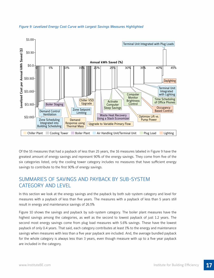
COST CURVEBased upon the net present value (NPV) of each measure, we found the levelized cost per annual kWh saved for each measure and organized measures into an annual marginal kWh saved curve (Figure 9). A negative cost on the curve means that there is a positive net present value for that particular measure.

The marginal kWh saved curve shows the levelized cost per annual kWh saved of each measure on the y axis. (Only the 55 measures with a payback of less than 25 years were included, as in previous charts.) Levelized cost per annual kWh saved was calculated by taking the negative of the NPV and dividing that by the annual kWh that would be saved through that measure. On the x-axis, the marginal annual kWh saved by each measure is shown. The width of each bar represents the total annual percent kWh saved by each measure. (kWh was used to normalize total energy units of electricity, gas and other fuels. The energy savings calculations in this example are not adjusted for the ways in which measures will interact with each other, actual energy savings may be lower.) Labeled measures are the measures that provide the largest amount of energy savings. They account for 90 percent of the total kWh saved by all measures. The bars without labels account for the remaining 10 percent of energy savings. To keep the scale of the graph readable, three measures with very high levelized cost were excluded: automatically controlled shading, electrochromic windows, and air handling unit device sub-metering.

17www.InstituteBE.com Institute for Building Efficiency

Figure 9: Levelized Energy Cost Curve with Largest Savings Measures Highlighted

0 5% 10% 15% 20% 25% 30% 35% 40% 45%

$1.00

$0.50

$0.0

$(0.50)

$(1.00)

$(1.50)

$(2.00)

Leve

lized

Cos

t pe

r A

nnua

l kW

h Sav

ed (

$)

Zone SetpointLimiting

Annual kWh Saved (%)

Terminal Unit Integrated with Plug Loads

OccupancyBased ControlDemand Control

Ventilation

Zone SchedulingIntegrated into

Building Scheduling

Waste Heat RecoveryUsing a Stack Economizer

ActivateComputer

Sleep Savings

Daylighting

Upgrade to Variable Primary FlowDemand

Response usingThermal Mass

Time Schedulingof Office Phones

Terminal UnitIntegrated

with Lighting

Boiler StagingChiller VSD

Upgrade

Optimize Lift vs.Pump Power

ComputerMonitor

BrightnessControl

Air Handling Unit/Terminal UnitBoiler PlantChiller Plant Plug Load LightingCooling Tower

Of the 55 measures that had a payback of less than 25 years, the 16 measures labeled in Figure 9 have the greatest amount of energy savings and represent 90% of the energy savings. They come from five of the six categories listed, only the cooling tower category includes no measures that have sufficient energy savings to contribute to the first 90% of energy savings.

SUMMARIES OF SAVINGS AND PAYBACK BY SUB-SYSTEM CATEGORY AND LEVELIn this section we look at the energy savings and the payback by both sub-system category and level for measures with a payback of less than five years. The measures with a payback of less than 5 years still result in energy and maintenance savings of 26.5%

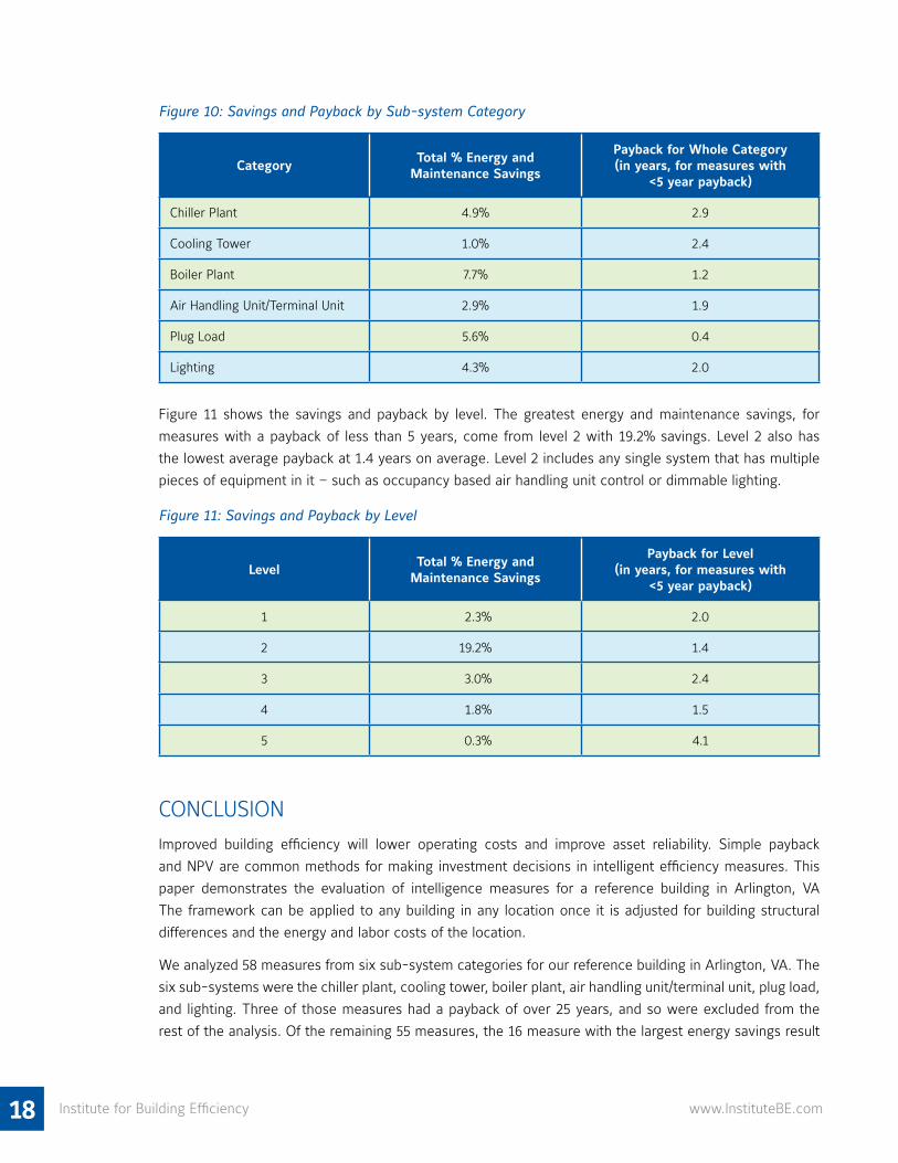
Figure 10 shows the savings and payback by sub-system category. The boiler plant measures have the highest savings among the categories, as well as the second to lowest payback of just 1.2 years. The second most energy savings come from plug load measures with 5.6% savings. These have the lowest payback of only 0.4 years. That said, each category contributes at least 1% to the energy and maintenance savings when measures with less than a five year payback are included. And, the average bundled payback for the whole category is always less than 3 years, even though measure with up to a five year payback are included in the category.


Figure 10: Savings and Payback by Sub-system Category

Category Total % Energy and Maintenance Savings

Payback for Whole Category (in years, for measures with

<5 year payback)

Chiller Plant 4.9% 2.9

Cooling Tower 1.0% 2.4

Boiler Plant 7.7% 1.2

Air Handling Unit/Terminal Unit 2.9% 1.9

Plug Load 5.6% 0.4

Lighting 4.3% 2.0

Figure 11 shows the savings and payback by level. The greatest energy and maintenance savings, for measures with a payback of less than 5 years, come from level 2 with 19.2% savings. Level 2 also has the lowest average payback at 1.4 years on average. Level 2 includes any single system that has multiple pieces of equipment in it – such as occupancy based air handling unit control or dimmable lighting.

Figure 11: Savings and Payback by Level

Level Total % Energy and Maintenance Savings

Payback for Level (in years, for measures with

<5 year payback)

1 2.3% 2.0

2 19.2% 1.4

3 3.0% 2.4

4 1.8% 1.5

5 0.3% 4.1

CONCLUSIONImproved building efficiency will lower operating costs and improve asset reliability. Simple payback and NPV are common methods for making investment decisions in intelligent efficiency measures. This paper demonstrates the evaluation of intelligence measures for a reference building in Arlington, VA The framework can be applied to any building in any location once it is adjusted for building structural differences and the energy and labor costs of the location.

We analyzed 58 measures from six sub-system categories for our reference building in Arlington, VA. The six sub-systems were the chiller plant, cooling tower, boiler plant, air handling unit/terminal unit, plug load, and lighting. Three of those measures had a payback of over 25 years, and so were excluded from the rest of the analysis. Of the remaining 55 measures, the 16 measure with the largest energy savings result

19

8 Whitestone Facility Operations Cost Reference 2012 - 2013, North American Edition, Whitestone Research.


in 90% of the total potential savings. These 16 come from each of the six categories except the cooling tower, which had no measure that resulted individually in a high percent energy savings.

The 47 measures with less than a 5 year payback still result in energy and maintenance savings of 26.5%. The greatest portion of those savings come from measures in level 2, with 19.2% savings from just that level for measure with less than a 5 year payback.

While this paper does not include the way that measures may interact with each other in our calculations of energy savings, it clearly shows that large improvements in the energy efficiency of buildings are possible through the installation of intelligent building technologies. 90% of the efficiency gains and maintenance savings in our reference building come from a group of just 16 measures that are at level 2, i.e. they improve single systems with multiple pieces of equipment in them. These 16 measures are spread across a variety of sub-system categories.

APPENDIX 1: ASSUMPTIONS

Costs

Improvement costs include both hard costs and soft costs. The hard costs consist of new equipment that needs to be added to the system to realize the improvement. Soft costs consist of the labor to configure or program an improvement in the building automation system (BAS). Due to the type of building modeled, it is assumed that a BAS is already installed and operating.

The hard cost of an improvement is assumed to be the retail cost of the equipment installed plus the installation cost of the equipment being installed by trained professionals.

The soft cost of an improvement is assumed to be the labor cost of an Energy Utility Operator,8 multiplied by an estimate of the amount of time to implement a change.

Savings

For those measures that will result in maintenance savings, maintenance cost savings are assumed to be proportional to the energy savings of any improvement, since the equipment is operating for fewer hours or at a lower output. The amount of maintenance savings is the maintenance cost of the particular equipment multiplied by the percent energy savings of the improvement.

Electrical and thermal energy cost savings should be calculated based on the cost of energy and the expected efficiency gains from each improvement being considered.

APPENDIX 2: INTELLIGENCE MEASURESMore detailed descriptions of each intelligence category and measure, along with an outstanding set of references for each, are listed here.

CHILLER PLANTThere are two primary types of chillers; mechanical compression chillers and absorption chillers. Chillers have multiple components comprising two fluid loops: the cold water loop that feeds the air handling units and the waste heat loop that circulates through the cooling tower.

20

9 Predictive and Diagnostics Methods for Centrifugal Chillers, Jayaprakash Saththasivam, ASHRAE Transactions, Volume 114, Part 1, 2008.

10 Case Study: The ROI of Cooling System Energy Efficiency Upgrades, Whitepaper #39, The Green Grid, 2011.

11 Submetering of Building Energy and Water Usage, Analysis and Recommendations of the Subcommittee on Buildings Technology Research and Development, National Science and Technology Council Committee on Technology, October 2011.

12 Ibid.

13 ARTI-21CR/611-20070-01, Variable Primary Flow Chilled Water Systems: Potential Benefits and Application Issues, Final Report, Volume 1, March 2004 Air-Conditioning and Refrigeration Technology Institute.

14 Variable Primary Flow Chilled Water Systems: Potential Benefits and Applications, Final Report, Volume 1, ARTI-21CR/611-20070-01, The Pennsylvania State University, 2004.


The main equipment components of a chiller plant include:

• Cooling tower

• Chilled water valves

• Chiller

– Condenser

– Compressor

– Evaporator

• Condenser water pump

• Chilled water pump

A brief description of the strategies for improving the intelligence of chillers follows:

Level 1: Equipment and components

• Modeling of thermal resistance vs. internal entropy. Apply a simple thermodynamic model of a chiller over time and determine if the thermal resistance and/or internal entropy have exceeded thresholds to indicate chiller faults.9

Level 2: Subsystems

• Chiller device submetering. Meter and trend the electrical power consumption of the chiller and alarm on power exceeding statistically expected bounds.

• Chiller equipment estimating diagnostics. Trend the estimated power consumption, provided by the chiller panel and alarm on power exceeding statistically expected bounds.

• Chiller sequencing. If a plant contains multiple chillers, the system monitors the load and turns on chillers in a sequence such that each one is part-loaded enough to keep it in its most efficient operating area.

• Chiller VSD upgrade. Upgrade the chilled water pumps with variable-speed drives (VSDs) to match the part-load characteristics of the chiller.

– Installation = 10 hrs/VSD10

– Unit cost $6,00011

– Savings = 6 kW, $4,53812

• Energy monitoring with outlier analysis. Monitor the plant capacity (Qevap) and predict the coefficient of performance (COP) of the chiller. Identify when the plant capacity or COP deviates from statistically expected performance.

• Upgrade to variable primary flow. Modify the chiller plant from a constant-flow system to a variable primary flow system. Variable primary flow uses a single set of pumps with variable-frequency drives to serve both the primary and secondary chilled water loop.

– Potential savings: Variable-flow systems reduce the total annual plant energy by 3 to 8 percent and lifecycle costs by 3 to 5 percent.13

– Estimated cost: Example upgrade from primary/secondary to variable flow is $27,671,14 using the Whitestone 2012 cost estimating tool, the cost is $40,500.

21

15 Best Practice for Energy Efficient Cleanrooms, Tengfang Xu, 2013, Lawrence Berkley National Laboratory.

16 LIT-12011575, Johnson Controls Central Plant Optimization™ 10 Application Note, May 13, 2011.

17 Introduction to Commercial Building Control Strategies and Techniques for Demand Response, Demand Response Research Center, Lawrence Berkley National Lab, May 2007.



Level 3: Cross-system

• Chilled water temperature reset based on outside air. Monitor outdoor conditions and reset the chilled-water temperature higher to the point just below where loads can no longer be satisfied.

– Potential savings: An increase of one degree in the chilled water supply temperature can increase the operational efficiency of the chiller by 1 to 2 percent.15

• Condenser water temperature reset based on outside air. Higher condenser water temperatures decrease cooling tower fan power but increase chiller power. The optimum operating temperature occurs at the point where these two opposing trends combine to produce the lowest total power use.

• Optimize lift vs. pump power. In a centrifugal chiller, constantly adjust the pump power to adjust the chiller part load to the point where the combination of the chiller energy consumption and pump energy consumption is minimized.

– Potential savings: Energy savings of up to 15 percent16 of pump power.

Level 4: Whole building

• Demand response using thermal mass. Reducing the energy consumption of a building during high demand times by precooling the building before the demand event. Cost savings are in the form of a utility incentive.

– Potential savings: 100 kW electric load reduction.17

– Potential energy cost: 4-hour precool of building @ $0.12/kWh

– Implementation cost: Installation of demand response signaling system.

• Model-based control. Since the cooling system of a commercial building consumes up to 55 percent of the building’s power, a model of the energy consumption over time can be used for planning purposes. The measure includes modeling of the chiller plant to predict the time-varying demand of the system and communicating this to a BAS or energy service provider (ESP) to use in ensuring electrical power during high-usage times.

• Utility meter integration. Submetering of the chiller to a BAS for monitoring, trending, and alarming.

– Potential Savings: Case study from the University of California and California State University stated, “The chiller and boiler also operated at night, performing simultaneous heating and cooling; the manual usage readings had not triggered any alarms that would have revealed this problem.”18

Level 5: Campus

• Integrated work order management. System integrates with a continuous diagnostics advisor (system that constantly monitors chiller plant systems to detect problems through abnormal energy consumption and identifies equipment faults) and automatically prioritizes and issues work orders to repair or replace faulty chiller equipment.

• Proactive maintenance. Preventive maintenance program that improves the reliability and efficiency of a chiller plant by predicting when components will fail and replacing them before failure.

22

19 Evaluating Peak Load Shifting Abilities and Regulation Service Potential of a Grid Connected Residential Water Heater, Harshal Upadhye, Ron Domitrovic, Ammi Amarnath, 2012 ACEEE Summer Study on Energy Efficiency in Buildings.

20 ENERGY STAR® Building Upgrade Manual, United States Environmental Protection Agency, Office of Air and Radiation, 2008 Edition.

21 Variable Speed Pumping, A Guide to Successful Applications: Executive Summary, U.S. DOE Industrial Technologies Program, January 2012.


COOLING TOWERCooling towers are mechanical equipment that provides a method to reject heat from a building’s cooling system to the atmosphere. Effective waste heat rejection is key to improving the efficiency of a chiller system. The main equipment of a cooling tower consists of:

• Water valve

• Spray Nozzles

• Suction screen

• Fan

• Condenser pump

A brief description of the strategies for improving the intelligence of a cooling tower follows:


• Tower flow metering of the cooling tower loop. Instrumenting the cooling tower system to monitor the condenser water flow, trending of the difference between the input and output flow, and alarming if the difference exceeds statistical norms.

• Tower temperature measurement of dispersion fan and condenser pump. Instrumenting the dispersion fan and condenser pump to monitor the motor temperatures, trending these temperatures, and alarming if the temperature exceeds statistical norms.

• Tower vibration analysis of dispersion fan and condenser pump. Instrumenting the dispersion fan to monitor the fan vibration and the condenser pump to monitor the pump vibration, trending of theses vibrations, and alarming if the vibrations exceed statistical norms.


• Conductivity controller retrofit. A conductivity controller measures the conductivity of the cooling tower water and discharges water only when the conductivity set point is exceeded.

– Potential savings: Annual water savings with a new cooling tower conductivity controller can be as much as 40 percent. In a large building, this translates into a $1,300 savings in water, chemical, and filter costs.19

• Multiplexing of multiple cooling towers. In systems with more than one cooling tower, run condenser water over as many towers as possible, at the lowest possible fan speed, and as often as possible to extract the most heat.

– Potential savings: The chiller will consume 2.5 to 3.5 percent more energy for each degree increase in the condenser temperature.20

• Upgrade constant-speed fan to variable-speed fan. Change a constant-speed fan to a variable-speed fan to reduce energy by varying the fan speed to match the load and the temperature difference between the condenser water and the outside air temperature.

– Potential savings: Savings of 30 to 50 percent of fan energy have been achieved in many installations by installing VSDs.21

23

22 Variable Speed Pumping, A Guide to Successful Applications: Executive Summary, U.S. DOE Industrial Technologies Program, January 2012Variable Speed Pumping, A Guide to Successful Applications, US Department of Energy, Industrial Technologies Program, May 2004.


24 Operations & Maintenance Best Practices, Version 3.0, US Department of Energy, August 2010.

25 Ibid.

26 Ibid.


• Upgrade constant-speed condenser pump to variable-speed pump. Change a constant-speed pump to a variable-speed pump to reduce energy by varying the pump speed to match the load and temperature difference between the condenser water and the outside air temperature.

– Potential savings: Savings of 30 to 50 percent of pump energy have been achieved in many installations by installing VSDs.22

BOILER PLANTTwo types of equipment are used to provide central heat for buildings: boilers and furnaces. Boilers, which produce hot water or steam that is then distributed throughout a building, heat about 32 percent23 of all U.S. commercial floor space. While furnaces and other heating systems provide the remainder of the heat facilities for commercial buildings, they do not provide a significant energy savings opportunity. The main equipment components of a boiler plant include:

• Burner (or electric heating element)

• Pressure sensor

• Water tubes

• Water pump

• Temperature sensor

A brief description of the strategies to improve boiler intelligence follows:


• Boiler carbon monoxide (CO) detection. Instrument the boiler flue to monitor carbon monoxide, trend the value, and alarm if the CO level exceeds statistical norms.

• Combustion monitoring. Ensure that the burner fuel-to-oxygen mix is correct to improve combustion efficiency.

– Potential savings: A 3 percent decrease in flue gas O2 typically produces boiler fuel savings of 2 percent.24

Level 2: Subsystems

• Boiler equipment estimating diagnostics (electric boilers). Trend the estimated power consumption, provided by the boiler panel, and alarm on power exceeding statistically expected bounds.

• Boiler staging. In systems that have multiple boilers, stage the boilers to ensure that the system load matches the boiler output to reduce boiler cycling.

– Potential savings: Matching of boiler size and boiler load can save as much as 50 percent of a boiler’s fuel use.25

• Electric boiler device submetering. Meter and trend the electrical power consumption of the boiler and alarm on power exceeding statistically expected bounds.

• Waste heat recovery using a stack economizer. Reduce the amount of heat being lost through the flue by installing a waste heat recovery system to preheat boiler feedwater.

– Potential savings: Stack losses for boilers without recovery are about 18 percent for gas-fired and about 12 percent for oil- and coal-fired boilers.26

24


28 Energy Savings Modeling of Standard Commercial Building Retuning Measures: Large Office Buildings, N Fernandez, Pacific Northwest National Laboratory (PNNL), June 2012.




• Energy monitoring with outlier analysis. Use statistical peer analysis to determine boiler performance. Alarm on boilers that are performing significantly worse than others.

• Hot water or zone temperature reset. Reset the boiler temperature based on the zone temperature. When heating loads decrease, the temperature of the hot water is decreased, reducing energy consumption.

• Utility meter integration (electric boilers). Submeter the boiler using a BAS for monitoring, trending, and alarming.

– Potential savings: Case study from the University of California and California State University identified “The chiller and boiler also operated at night, performing simultaneous heating and cooling; the manual usage readings had not triggered any alarms that would have revealed this problem.”27

– Potential savings: Every 4°F the boiler water temperature is reduced leads to 1 percent energy savings.28

• Grid regulation exploiting thermal mass (electric boilers). Modulate the boiler temperature based on a signal from the electric grid. This is used to increase the reliability of the electric grid. A customer is provided an incentive by the utility for participation.

AIR HANDLING/TERMINAL UNITSAir distribution systems bring conditioned air to the occupants of a building. There are two types of air-handling systems: constant volume (CV) and variable air volume (VAV). In a CV system, a constant amount of air flows through the system whenever it is on. A VAV system changes the amount of airflow in response to changes in the heating and cooling load. In this analysis, the building is assumed to contain a VAV system. On average, the fans that move conditioned air through commercial office buildings account for about 7 percent of the total energy consumed by these buildings,29 so reductions in fan consumption can result in significant energy savings. The main equipment components of an air handling unit include:

• Supply and return fans

• Outside air, return air and exhaust air mixing dampers

• Steam and cooling valves

• Heating and cooling coil

• Heat exchanger

• Humidifier

• Humidity, temperature, flow, status and pressure sensors

• Filter

25


31 Demand Control Ventilation using CO2 Sensors, Federal Technology Alert, US Department of Energy, 2004.




A brief description of the strategies to improve the intelligence of an air handling unit or terminal unit follows:


• AHU fan pressure detection. This measure provides supervision of the fan to ensure that the fan is providing duct static pressure.

• AHU fan pressure measurement. This measure trends the duct static pressure and alarms when the system is outside normal tolerances.

Level 2: Subsystems

• Lower VAV minimum flow rate – Lower the minimum air flow rate at each VAV terminal to 30 percent of the maximum flow unless the system violates the ASHRAE minimum airflow standards.

– Potential savings: For post-1980 buildings, the HVAC savings range from 15 to 25 percent from lowering the minimum airflow set point from 40 percent to 30 percent.30

• Demand-controlled ventilation. In a DCV system, sensors monitor the CO2 levels inside and send a signal to the HVAC controls, which regulate the amount of outside ventilation air that is drawn into the building. Though ASHRAE does not set a maximum allowable CO2 concentration, the most recent version of the standard recommends that the indoor CO2 level be no more than 700 parts per million (ppm) above the outside level, which is typically about 350 ppm.

– Potential savings: The potential of CO2-based DCV for operational energy savings has been estimated in the literature from $0.05 to more than $1 per square foot annually.31

• Device submetering. Meter and trend the electrical power consumption of the AHUs and alarm on power exceeding statistically expected bounds.

• Duct static pressure reset. Pressure reset can yield additional energy savings in systems that have VSDs installed. By ensuring that the warmest zone is satisfied, the other zones can open fully to keep them satisfied.

• Economizer cooling. Air-side economizers consist of a collection of dampers, sensors, actuators, and logic devices on the supply-air side of the air-handling system. The outside-air damper is controlled so that when the outside air temperature is below a predefined setpoint, the outside-air damper opens, allowing more air to be drawn into the building. On hot days, the economizer damper closes to its lowest setting, which is the minimum amount of fresh air required by the local building code.

– Potential savings: This measure is most effective in regions that have a cooler shoulder season. The total savings range from a low of 2 percent in Miami to a high of 19 percent in Duluth, Minn.)32.

• Equipment estimating diagnostics. Trend the estimated power consumption, provided by the AHU controller, and alarm on power exceeding statistically expected bounds.

– Potential savings: The post-1980 baseline shows higher savings than the pre-1980 baseline because fan energy consumption is a higher fraction of overall HVAC consumption in the post-1980 baseline. Post-1980 savings range from 5 to 7 percent.33

26

34 Ibid.

35 Strategies for Demand Response in Commercial Buildings, David S. Watson, Sila Kiliccote, Naoya Motegi, and Mary Ann Piette, Lawrence Berkeley National Laboratory, 2006 ACEEE Summer Study on Energy Efficiency in Buildings.

36 Ibid.


• Network scheduled control. A zone is set to an energy savings condition during the times outside of the normal work day. This is sometimes called setback or time-clock control.

• Enthalpy-based control. Outdoor temperature and humidity are compared against a predetermined enthalpy setpoint to determine how much outdoor air to accept into the AHU system. In humid climates, up to 50 percent of the cooling system’s energy is used to dehumidify conditioned air.

• Occupancy-based Control. Reset zone setpoints to an energy savings condition when an occupancy sensor indicates that the zone is unoccupied. Reduce the outdoor air flow rate to zero when the building is unoccupied.

– Potential savings: The savings are climate-dependent. In the coldest climates, the heating savings may be as much as 5 to 6 percent.


• AHU zone scheduling integrated into building scheduling. This measure commands the AHU to revert to nighttime setback mode two hours earlier in the evening on weekdays, letting the building coast toward its unoccupied state while it is still partially occupied.

– Potential savings: In simulations, this measure keeps the HVAC systems completely off unless the boilers or chillers turn on to maintain the zones at the setback temperatures. In total, this reduces the HVAC system “on” time by 22 hours, out of a total of 92 hours in the baseline. Most locations show HVAC savings close to 24 percent.34

• Terminal unit integrated with lighting. The lighting in a zone is controlled by the VAV terminal occupancy status. The occupancy status is set via an occupancy sensor in the zone.

• Terminal unit integrated with plug loads. The outlets in a zone are controlled by the VAV terminal occupancy status. The occupancy status is set via an occupancy sensor in the zone.

• Zone scheduling integrated into building scheduling. This measure commands the VAV damper to close when the building is unoccupied.

• Zone scheduling integrated into security system. Turn off the AHU in zones where the security system indicates there are no occupants. The security system would need to be “location aware” of the occupants.


• AHU fan limiting. Increase the zone temperature setpoints for an entire facility to provide demand response.

– Potential savings: Global setpoint limiting has potential to save up to 0.5 W/sq-ft in energy35 during a demand response event.

• Zone setpoint limiting. Increase the zone temperature setpoints for an entire facility to provide demand response.

– Potential Savings: Global setpoint limiting has potential to save up to 0.5 W/sq-ft in energy36 during a demand response event.

27

37 Program Requirements for Imaging Equipment – Eligibility Criteria V2.0, EPA ENERGY STAR, Jun-2013.

38 Plug Load Best Practices Guide, New Buildings Institute, undated.

39 Ibid.

40 Massachusetts Market Assessment and Best Practices for Delivering Plug-Load Energy Efficiency in Businesses-Final Report, PA Knowledge Limited, June 14, 2010.

41 Ibid.


PLUG LOADSThere are two primary types of plug loads: primary loads connected directly to the electrical system of the building, and secondary loads connected to the building electrical system through a power strip. The distinction between these two types of loads is based on the capability to perform power management on the load. A primary load is a stationary device that would be expected to be sophisticated enough to be able to manage its own energy consumption. Examples include printers, refrigerators, televisions and vending machines. A secondary load is typically a low-cost device that would not be expected to be able to manage its own energy consumption. Examples include task lighting, power-supply bricks for laptop computers, phone chargers and space heaters.

Many primary loads in a building are already developed to improve the energy efficiency of a building by meeting U.S. EPA ENERGY STAR® ratings. Launched by the EPA in 1992 and supported in over 40,000 individual products, the ENERGY STAR program was designed to promote cost-effective, innovative solutions for reducing GHG emissions. The program has boosted the adoption of energy-efficient products, practices, and services through valuable partnerships, objective measurement tools, and consumer education. The purchase of products rated by ENERGY STAR should be the first measure adopted to reduce the energy consumption of a smart building’s plug loads. A brief description of the strategies for improving the intelligence of plug loads follows:

Level 1: Equipment and Components

• Batch printing. Networked printers rated ENERGY STAR v1.2 and above are designed with multiple operational modes that each consume different amounts of power. The ON mode has two sub-modes: an “active-state” sub-mode used when printing, and a “ready-state” used when the printer is waiting for a print job.37 In a typical piece of printing equipment, the ready-state power consumption is 64 percent less than the active-state power. In this measure, only time-sensitive material is printed on demand while other print jobs are batched together and printed at some periodic rate. This increases the amount of time that the equipment is in the ready-state, saving energy.

– Typical active-state power draw = 185 W38

– Typical ready-state power draw = 66 W39

– Density: 1 piece of imaging equipment per 75 occupants

– Active-state time reduction: 1 hr/day

• Time scheduling of cold beverage vending machines. A plug load device turns off the vending machine when the building becomes unoccupied. There is a significant energy savings opportunity of 1,300 kWh annually for retrofitting conventional cold beverage machines.40 A conservative schedule is to have the vending machines on for 12 hours a day during the week and off for weekends and holidays. Stand-alone devices for this function cost $100 to $190.41

– Density: 1 beverage machine for each 250 occupants

– Savings: 1,300 kWh per machine/yr

– Electric rate: $0.20/kWh

28

42 Ibid.

43 Plug-Load Control and Behavioral Change Research in GSA Office Buildings, National Renewable Energy Laboratory, June 2012.






• Time scheduling of non-perishable vending machines. Install a device to turn off power to the vending machines when the surrounding area is vacant. A non-refrigerated vending machine consumes about 360 kWh/year of energy. Stand-alone devices for this function cost $70 to $80.42

– Density: 1 snack machine for each 250 occupants

– Savings: ___ kWh per machine/yr


• Time scheduling of office phones. Newer Voice Over IP (VOIP) phones draw on average 2 W.43 Since they are typically powered from the network, the router can be scheduled to turn off the power to the phones during off-hours. Incoming calls will be directed to voicemail when the phones are powered down to avoid lost calls. A conservative schedule is to have the phones on for 12 hours a day during the week and off on weekends and holidays.

– Density: 1 phone per occupant, 1 IP router for every 5,000 sq-ft of building

– Savings: ___ kWh per phone/year


Level 2: Subsystems

• Activate computer sleep savings. Activate the sleep settings of computers to reduce the active-state time when not being used. ENERGY STAR recommends that computers sleep after 15 to 60 minutes of inactivity; many laptops allow a more aggressive setting of 3 to 5 minutes to extend battery life. In addition, monitors can be dimmed during shorter periods of inactivity to increase energy savings.

– Density = 1 computer per occupant

– Implementation: By IT network setting. Uptake of 100 percent using policy setting application with $10/user/year licensing fee.44

– Savings = $50/yr45 or 200 kWh46 per computer

• Computer monitor brightness control. Due to the way human eyes perceive light, the brightness of a computer monitor can slowly be reduced to save power and will not be noticed by the user. Energy savings of 17 percent can be attained before the change in brightness becomes noticeable.47 This measure sets a policy that all LED monitors be configured to reduce screen brightness to the ENERGY STAR energy savings level.

– Power Consumption: LED Monitor, 18 W

– Implementation: Policy and support = $2,500

– Density: 1 monitor per occupant

29

48 Navigant Research, Smart Glass: Electrochromic, Suspended Particle, and Thermochromic Technologies for Architectural and Transportation Applications: Global Market Analysis and Forecasts. 2013.

49 http://venturebeat.com/2013/08/19/heliotrope-smart-glass/

50 Reinhart, C.F. (2002) Effect of interior design on the daylight availability in open plan offices. National Research Council of Canada, Internal Report NRCC-45374, NRC: Ottawa.

51 Huang, J. et al. (2006) “Preliminary evaluation of the energy saving potentials of exterior operable window shading systems for residential buildings in California climates” LBNL.


LIGHTINGBuilding lighting systems can be made more intelligent and efficient by ensuring that maximum daylight is used when available, and that lights are dimmed or turned off when they are not needed. Daylight can be maximized through the use of automatically controlled shading or electrochromic glass. Lights can be dimmed and turned off in response to available daylight with photosensors. Dimming of fluorescent lights is enabled by installing electronic ballasts. Occupancy sensors can enable lights to be turned off altogether when a space is unoccupied. A brief description of the strategies for improving the intelligence of lighting follows:


• Electrochromic (EC) windows. EC windows have coatings that allow them to darken and lighten upon the application of a very small electric voltage. With the proper sensors and control algorithms, an EC window system in a large commercial building can automatically darken the windows when the sun is high and its rays are heating the interior, thus reducing the solar heat gain and the need for air conditioning. As the sun sets or clouds cover the sky, the system would move the windows back toward transparency, maximizing daylighting and reducing the use of electric lighting. Early studies at Berkeley Lab suggested they could reduce a commercial building’s annual lighting energy use from a few percent to roughly 25 percent or more. Cooling energy savings aren’t included here but would be significant. We will assume 15 percent savings for this paper. Only the fluorescent portion lighting (71 percent) is included in the calculation, since it is dimmable.

– Window area: 40 percent, since the reference building was built before 1980. The percent windows assumption is dependent on building structure and design elements.

– Cost per square foot of window: $45 to $70,48 median $57

– Installation cost: $143 per square foot49

Level 2: Subsystems

• Automatically controlled shading. A system that automatically controls the window shades in response to the amount of daylight can result in significant energy savings. Savings for automatic systems vary widely depending on the size and type of windows and the size of the office. Having automatic shades instead of manually adjustable shades (which occupants may often leave down during the day) can result in 20 percent additional energy savings on lighting by enabling additional dimming.50 Only the fluorescent portion lighting (71 percent) is included in the calculation, since it is dimmable.

– Windows area: 40 percent since the reference building was built before 1980. The percent windows assumption is dependent on building structure and design elements.

– Installation: $48/sq-ft51

30

52 http://www-is.informatik.uni-oldenburg.de/~dibo/teaching/mm/pages/light-fundamentals.html#ballestsNLPIP. (2000) “Electronic Ballasts: Non-dimming electronic ballasts for 4-foot and 8-foot fluorescent lamps”. Volume 8, Number 1. RPI.


• Daylighting. Dimmable lighting fixtures enable daylighting, saving energy in two ways, first by using efficient electronic ballasts, second by dimming the lights below full output when daylight is available, which are:

(1) Electronic ballast conversion. Controllable electronic ballasts replace magnetic ballasts for fluorescent lights. They increase lamp-ballast efficacy, leading to increased energy efficiency and lower operating costs. Electronic ballasts operate lamps using electronic switching power supply circuits. Electronic ballasts take incoming 60 Hz power (120 or 277 volts) and convert it to high-frequency AC (usually 20 to 40 kHz). By converting input power to the proper lamp power, they operate fluorescent lamps at higher frequencies, reducing end losses. Lamps operating at these higher frequencies produce about the same amount of light, while consuming 10 to 25 percent less power.52 A median of 15 percent will be assumed for this study.

– Density: 1 ballast per fluorescent light, minimum lighting density = 1.2 W/ft2. Assuming 120 W fixtures, the reference building would need 250 fixtures. In a typical office building, lighting is close to the number of VAV terminals (600). Assume 600 for the reference building.

– Cost = Ballast Cost + Installation Cost. Assume $20/ballast and $250/ballast installation for $270 total.

(2) Electronic ballasts also enable fault detection and dimming for florescent lighting. Dimming can reduce lighting levels to their lowest acceptable level and reduce lighting at times when daylight is abundant. Photosensor-controlled lights with continuous dimming from 40 to 100 percent of full output, use about half as much electricity as standard non-dimmable fixtures. The overall savings will be somewhat less due to occasional overcast conditions, shorter days during the winter, and the fact that daylighting is not possible for the interior space, resulting in an actual lighting energy savings of 32 percent. Only the fluorescent portion lighting (71 percent) is included in the calculation since it is dimmable.

– Density: In a typical office building, lighting is close to the number of VAV terminals (600). Assume 600 for the reference building.

– Cost = Photo sensor + Installation Cost. Assume $1/photo sensor and $250/ballast installation to enable dimming for $251 total.

• Occupancy-based control. Occupancy-based control is one of the most effective energy savings opportunities. It covers times when a space is unoccupied during a normally occupied period and when a facility is unoccupied outside the normal work day, including evenings, weekends and holidays. The energy savings from occupancy sensors vary significantly depending on the level of occupancy and how well occupants already do at turning off lights in unoccupied spaces. The EPA says installing occupancy-based lighting controls will save 13 to 50 percent in a private office; the Electric Power Research Institute says the average is 25 percent% savings . Higher savings are often seen in conference rooms and corridors that are occupied less of the time.

– Density: 1 sensor per 1,000 sq-ft

– Sensor cost $20. Installation cost $250/sensor.

– Savings: 25 percent lighting energy savings

© 2014 Johnson Controls, Inc. 444 North Capitol St., NW Suite 729, Washington DC 20001 Printed in USAwww.johnsoncontrols.com

The Institute for Building Efficiency is an initiative

of Johnson Controls providing information and

analysis of technologies, policies, and practices

for efficient, high performance buildings and smart

energy systems around the world. The Institute

leverages the company’s 125 years of global

experi ence providing energy efficient solutions for

buildings to support and complement the efforts of

nonprofit organizations and industry associations.

The Institute focuses on practical solutions that are

innovative, cost-effective and scalable.

If you are interested in contacting the authors, or

engaging with the Institute for Building Efficiency,

please email us at: [email protected].

www.institutebe.com

intelligent efficiency - building efficiency initiative · intelligent efficiency ... simple...

Documents