intelligent manet optimisation system - open access...
TRANSCRIPT

________________________________________________________________________ii
Brunel University
School of Engineering and Design Electronic and Computer Engineering Department
Intelligent MANET Optimisation System
by Nagham Saeed
A thesis submitted for the degree of Doctor of Philosophy
February 2011

__________________________________________________________________ii
Abstract In the literature, various Mobile Ad hoc NETwork (MANET) routing protocols proposed. Each performs
the best under specific context conditions, for example under high mobility or less volatile topologies. In
existing MANET, the degradation in the routing protocol performance is always associated with changes
in the network context. To date, no MANET routing protocol is able to produce optimal performance
under all possible conditions.
The core aim of this thesis is to solve the routing problem in mobile Ad hoc networks by introducing an
optimum system that is in charge of the selection of the running routing protocol at all times, the system
proposed in this thesis aims to address the degradation mentioned above. This optimisation system is a
novel approach that can cope with the network performance’s degradation problem by switching to other
routing protocol. The optimisation system proposed for MANET in this thesis adaptively selects the best
routing protocol using an Artificial Intelligence mechanism according to the network context.
In this thesis, MANET modelling helps in understanding the network performance through different
contexts, as well as the models’ support to the optimisation system. Therefore, one of the main
contributions of this thesis is the utilisation and comparison of various modelling techniques to create
representative MANET performance models. Moreover, the proposed system uses an optimisation method
to select the optimal communication routing protocol for the network context. Therefore, to build the
proposed system, different optimisation techniques were utilised and compared to identify the best
optimisation technique for the MANET intelligent system, which is also an important contribution of this
thesis.
The parameters selected to describe the network context were the network size and average mobility. The
proposed system then functions by varying the routing mechanism with the time to keep the network
performance at the best level. The selected protocol has been shown to produce a combination of: higher
throughput, lower delay, fewer retransmission attempts, less data drop, and lower load, and was thus
chosen on this basis. Validation test results indicate that the identified protocol can achieve both a better
network performance quality than other routing protocols and a minimum cost function of 4.4%. The Ad
hoc On Demand Distance Vector (AODV) protocol comes in second with a cost minimisation function of
27.5%, and the Optimised Link State Routing (OLSR) algorithm comes in third with a cost minimisation
function of 29.8%. Finally, The Dynamic Source Routing (DSR) algorithm comes in last with a cost
minimisation function of 38.3%.

_____________________________________________________________________iii
Table of Contents
Chapter 1 ..........................................................................................................................................1 Introduction ......................................................................................................................................1 1.1 Introduction ..........................................................................................................................1 1.2 Motivation ............................................................................................................................2
1.2.1 Better MANET.............................................................................................................2 1.2.2 MANET Routing Problems..........................................................................................2
1.3 Research Aim and Objectives ..............................................................................................4 1.4 Challenges ............................................................................................................................5 1.5 Main Contributions ..............................................................................................................5
1.5.1 Comprehensive Taxonomy of Mobile Ad hoc Routing Protocols ...............................5 1.5.2 Creating and Comparing MANET Models ..................................................................6 1.5.3 Optimisation Techniques in MANET ..........................................................................6 1.5.4 Detailed Design and Implementation of the Optimisation System..............................6 1.5.5 Quantitative Evaluation of the Network Performance .................................................6 1.5.6 Test the Topology Packets Inter-Arrival Time ............................................................7
1.6 Thesis Scope.........................................................................................................................7 1.7 Thesis Outline ......................................................................................................................8 1.8 References ..........................................................................................................................10 Chapter 2 ........................................................................................................................................12 MANET Routing Protocols............................................................................................................12 2.1 Introduction ........................................................................................................................12 2.2 The Mobile Network Topology..........................................................................................13
2.2.1 Mobile Internet Network............................................................................................13 2.2.2 Mobile Ad hoc Network (MANET)...........................................................................14
2.2.2.1 MANET Functionality ............................................................................................14 2.2.2.2 Ad hoc Network History .........................................................................................15
2.3 Routing Protocols...............................................................................................................17 2.3.1 Routing in Wired Network.........................................................................................18 2.3.2 Routing in Wireless Ad hoc Network ........................................................................19
2.4 MANET Routing Protocols Taxonomy .............................................................................20 2.4.1 Design Philosophy......................................................................................................20
2.4.1.1 Proactive Routing Algorithm .................................................................................21 2.4.1.2 Reactive Routing Algorithm ...................................................................................22 2.4.1.3 Hybrid Routing Algorithm......................................................................................24
2.4.2 Network Structure ......................................................................................................25 2.4.2.1 Flat Routing............................................................................................................25 2.4.2.2 Hierarchical Routing..............................................................................................26 A. Zone-based (Hybrid) ......................................................................................................26 B. Cluster-based..................................................................................................................26 C. Core Node-based ............................................................................................................27 2.4.2.3 Geographic Position Information Assisted Routing...............................................27

_____________________________________________________________________iv
2.4.3 Casting Packets ..........................................................................................................27 2.4.3.1 Unicast Routing......................................................................................................28 2.4.3.2 Multicast Routing ...................................................................................................29 2.4.3.3 Broadcasting Methods............................................................................................30
2.4.4 Network Routing Metrics...........................................................................................31 2.5 Summary ............................................................................................................................32 2.6 References ..........................................................................................................................33 Chapter 3 ........................................................................................................................................37 Optimisation in MANET Routing Protocol ...................................................................................37 3.1 Introduction ........................................................................................................................37 3.2 MANET Routing Protocol Optimisation ...........................................................................37
3.2.1 Optimum Routing Protocols Based on Routing Metrics............................................38 3.2.1.1 Hop Count Metric...................................................................................................38 3.2.1.2 Context-Aware Metrics ..........................................................................................38
3.2.2 Optimum Routing Protocols Based on Prediction .....................................................40 3.2.3 Optimum Routing Protocols Based on Modelling /Prediction Techniques ...............40 3.2.4 Optimum Routing Protocols Based on Application Requirements............................41 3.2.5 Optimum Routing Protocols Based on Programmable Framework...........................41 3.2.6 Optimum Routing Protocols Based on Artificial Intelligence ...................................42
3.3 Related Work......................................................................................................................43 3.3.1 Models........................................................................................................................43 3.3.2 Prediction ...................................................................................................................44 3.3.3 Design.........................................................................................................................44 3.3.4 Objective ....................................................................................................................45
3.4 Summary ............................................................................................................................45 3.5 References ..........................................................................................................................46 Chapter 4 ........................................................................................................................................50 I-MAN Design................................................................................................................................50 4.1 Introduction ........................................................................................................................50 4.2 I-MAN Design Elements....................................................................................................51 4.3 MANET Routing Protocol Techniques..............................................................................55
4.3.1 OLSR Routing Protocol .............................................................................................55 4.3.2 DSR Routing Protocol Technique..............................................................................56 4.3.3 AODV Routing Protocol Technique ..........................................................................58 4.3.4 OLSR, DSR, and AODV Loop-Free Technique........................................................59 4.3.5 Comparison of OLSR, DSR, and AODV Routing Protocols.....................................60
4.3.5.1 Strengths of OLSR, DSR, and AODV Routing Protocols .......................................60 4.3.5.2 Weaknesses of OLSR, DSR, and AODV Routing Protocols ...................................62 4.3.5.3 Characteristics of OLSR, DSR, and AODV Routing Protocols .............................62
4.4 Summary ............................................................................................................................63 4.5 References ..........................................................................................................................64 Chapter 5 ........................................................................................................................................66 MANET Simulation .......................................................................................................................66 5.1 Introduction ........................................................................................................................66 5.2 MANET Simulations..........................................................................................................66
5.2.1 Communication Model...............................................................................................67

_____________________________________________________________________v
5.2.2 Movement Model .......................................................................................................67 5.2.3 Simulation Parameters................................................................................................68 5.2.4 Performance Evaluation Metrics................................................................................69
5.3 Simulation Results..............................................................................................................70 5.3.1 Averaging Data ..........................................................................................................70 5.3.2 Arranging Data Related to the Network Context .......................................................76 5.3.3 Results Analysis .........................................................................................................79
5.4 Summary ............................................................................................................................82 5.5 References ..........................................................................................................................83 Chapter 6 ........................................................................................................................................85 Modelling Methodology.................................................................................................................85 6.1 Introduction ........................................................................................................................85 6.2 Empirical Modelling ..........................................................................................................85
6.2.1 Regression Equation Models......................................................................................86 6.3 Artificial Intelligent Modelling Methods ...........................................................................87
6.3.1 Artificial Neural Networks Models............................................................................87 6.3.1.1 ANN Training Methods ..........................................................................................87 6.3.1.2 ANN Architecture Types.........................................................................................88 6.3.1.3 ANN Layers ............................................................................................................88 6.3.1.4 ANN Functions .......................................................................................................88
6.3.2 Neuro-Fuzzy Models..................................................................................................89 6.3.2.1 NF System Layers...................................................................................................90
6.4 MANET Models.................................................................................................................91 6.4.1 MANET Regression Models......................................................................................91 6.4.2 ANN MANET Models ...............................................................................................95 6.4.3 NF MANET Models.................................................................................................101 6.4.4 MANET Models Comparison ..................................................................................106
6.5 Summary ..........................................................................................................................108 6.6 References ........................................................................................................................109 Chapter 7 ......................................................................................................................................111 Intelligent Optimisation Techniques ............................................................................................111 7.1 Introduction ......................................................................................................................111 7.2 Intelligent Computing Optimisation Methods..................................................................112 7.3 Genetic Algorithm............................................................................................................113 7.4 PSO Algorithm.................................................................................................................118 7.5 Comparison between GA and PSO ..................................................................................121 7.6 Intelligent MANET Optimisation ....................................................................................122
7.6.1 Determined the Network Context Cases ..................................................................122 7.6.2 The Optimisers Configurations ................................................................................124 7.6.3 MANET Optimisation..............................................................................................124
7.6.3.1 GA MANET Optimiser .........................................................................................124 7.6.3.2 PSO MANET Optimiser .......................................................................................126
7.6.4 Creating the Validation Table ..................................................................................127 7.6.5 MANET Optimisers Selection .................................................................................128
7.7 Summary ..........................................................................................................................129 7.8 References ........................................................................................................................129

_____________________________________________________________________vi
Chapter 8 ......................................................................................................................................132 System Implementation................................................................................................................132 8.1 Introduction ......................................................................................................................132 8.2 I-MAN Optimisation System with MANET....................................................................133
8.2.1 Optimisation Unit in Intelligent Node......................................................................133 8.2.2 Embedding the Intelligent Unit in MANET Nodes .................................................135
8.3 Implementation.................................................................................................................135 8.4 MANET Nodes Modification...........................................................................................139
8.4.1 Creating the Intelligent Node ...................................................................................140 8.4.1.1 Embedding the Information Stack ........................................................................141 8.4.1.2 Embedding the NF Modeller ................................................................................141 8.4.1.3 Embedding the PSO Optimiser ............................................................................142 8.4.1.4 Embedding the Decision Maker ...........................................................................142
8.4.2 Creating the MANET Nodes....................................................................................142 8.5 Case Study........................................................................................................................144
8.5.1 Simulation Environment ..........................................................................................144 8.5.2 Experiment Configuration........................................................................................148 8.5.3 Simulation Results....................................................................................................150
8.6 Comparison and Results Analysis....................................................................................151 8.6.1 Data Drop .................................................................................................................151 8.6.2 Delay ........................................................................................................................152 8.6.3 Load..........................................................................................................................154 8.6.4 Retransmission Attempts (RA) ................................................................................155 8.6.5 Throughput ...............................................................................................................156
8.7 The Network Performance Cost Minimisation Equation.................................................157 8.8 The Performance Cost Minimisation Function Quantitative Evaluation .........................159 8.9 Studying the Inter-Arrival Time of Topology Packets.....................................................160 8.10 Case Study Limitations ....................................................................................................163 8.11 Summary ..........................................................................................................................165 8.12 References ........................................................................................................................166 Chapter 9 ......................................................................................................................................167 Conclusions and Future Work......................................................................................................167 9.1 Summary ..........................................................................................................................167 9.2 Conclusions ......................................................................................................................168 9.3 Achievements ...................................................................................................................169 9.4 Future Research................................................................................................................170
9.4.1 Short Term Future Research ....................................................................................170 9.4.1.1 Models Range .......................................................................................................170 9.4.1.2 Update Models .....................................................................................................170 9.4.1.3 Extend the Network’s Parameters........................................................................171 a. Context Parameter .......................................................................................................171 b. The Performance Parameter ........................................................................................171 c. The Routing Protocols..................................................................................................171 9.4.1.4 Add More Elements ..............................................................................................171 9.4.1.5 User Requirement.................................................................................................172 9.4.1.6 List of Intelligent Nominees..................................................................................172

_____________________________________________________________________vii
9.4.1.7 Partitioning the Network or Dropping the Protocol ............................................173 9.4.1.8 Hidden Nodes .......................................................................................................173 9.4.1.9 AI Technique ........................................................................................................174
9.4.2 Long-Term Future Research ....................................................................................174 9.4.2.1 Add Routing Protocol Classification List to I-MAN System ................................174 9.4.2.2 Context-aware routing protocol...........................................................................175 9.4.2.3 Wireless Mesh Network ........................................................................................175 9.4.2.4 Cognitive Network................................................................................................175 9.4.2.5 Intelligent Transportation Systems.......................................................................176 9.4.2.6 Internet of Things System .....................................................................................176 9.4.2.7 Real Test Bed........................................................................................................176 9.4.2.8 Expanding the System...........................................................................................176
9.5 References ........................................................................................................................177 Publications and Submissions Based on This Thesis................................................................... viii

_____________________________________________________________________viii
Publications and Submissions Based on
This Thesis
[1] N. H. Saeed, M. F. Abbod and H. S. Al-Raweshidy, “I-MAN: An Intelligent MANET routing
protocols optimization system,” IEEE Transactions on Mobile Computing, submitted on 7th of
February 2011.
[2] N. H. Saeed, M. F. Abbod and H. S. Al-Raweshidy, “Intelligent modelling of Ad hoc communication
network,” Applied Soft Computing, submitted on 2nd of March 2011.
[3] N. H. Saeed, M. F. Abbod, and H. S. Al-Raweshidy, “Intelligent MANET routing system,”
Processing of IEEE computer society, The 22nd International Conference on Advanced Information
Networking and Applications, WAINA - Workshops, pp. 1260-1265, Japan, 2007.
[4] N. H. Saeed, M. F. Abbod, H. S. Al-Raweshidy and O. Raoof, “Intelligent MANET routing
optimiser”, Fifth International Conference on Broadband Communications, Networks, and Systems,
Broadnets2008, London, UK, September 8-11, 2008.
[5] N. H. Saeed, M. F. Abbod, and H. S. Al-Raweshidy, “Modeling MANET utilising artificial
intelligent,” Processing of IEEE Computer Society, the 2nd UKSIM European Symposium on
Computer Modeling and Simulation, EMS2008, pp. 117-122, Liverpool, UK, 2008.
[6] N. H. Saeed, M. F. Abbod, T. H. Sulaiman, H. S. Al-Raweshidy, and H. Kurdi, “Intelligent MANET
routing protocol selector,” Processing of IEEE Computer Society, the Second International
Conference and Exhibition on Next Generations Mobile Applications Services and Technologies,
NGMAST‘08, pp. 389-394, Cardiff, Wales, UK, 2008.
[7] N. H. Saeed, M. F. Abbod, and H. S. Al-Raweshidy, “I-MAN: An Intelligent MANET routing
system”, The IEEE 17th International Conference on Telecommunications, ICT, Doha-Qatar, April 4 -
7, 2010.
[8] N. H. Saeed, M. F. Abbod and H. S. Al-Raweshidy, “MANET Modelling utilising Artificial
Intelligent,” ICCCA2011 conference, 2011.

_____________________________________________________________________ix
List of Figures
Figure 1.1: Thesis scope. ............................................................................................................................... 8 Figure 2.1: Mobile Internet classifications. ................................................................................................. 13 Figure 2.2: Mobile Ad hoc NETwork. ........................................................................................................ 15 Figure 2.3: MANET in battle field environment......................................................................................... 16 Figure 2.4: Routing protocol classifications for wired network.................................................................. 18 Figure 2.5: MANET routing protocol classifications depending on design philosophy. ............................ 21 Figure 2.6: Proactive routing algorithm Route discovery............................................................................ 22 Figure 2.7: Reactive routing algorithm Route discovery. ............................................................................ 22 Figure 2.8: MANET reactive routing protocol............................................................................................ 23 Figure 2.9: Hybrid-based routing algorithm................................................................................................ 24 Figure 2.10: MANET routing algorithms classifications depending on network structure. ....................... 25 Figure 2.11: Routing algorithm classifications depending on packet casting. ............................................ 28 Figure 2.12: Packets casting classification.................................................................................................. 28 Figure 2.13: Classifications of broadcast methodology. ............................................................................. 30 Figure 2.14: Routing protocol classifications depending on route metric................................................... 32 Figure 4.1: I-MAN routing protocols optimisation system block diagram. ................................................ 52 Figure 4.2: Flowchart for the I-MAN routing protocols optimisation system design. ................................ 54 Figure 4.3: An illustration of MPR nodes in the OLSR routing protocol. .................................................. 56 Figure 4.4: Formation of Route discovery in DSR. ..................................................................................... 57 Figure 4.5: AODV Route discovery. ........................................................................................................... 59 Figure 4.6: Loop technique. ........................................................................................................................ 60 Figure 5.1: OLSR, DSR, and AODV routing protocols data drop results. ................................................. 71 Figure 5.2: OLSR, DSR, and AODV routing protocols delay results......................................................... 72 Figure 5.3: OLSR, DSR, and AODV routing protocols load results........................................................... 73 Figure 5.4: OLSR, DSR, and AODV routing protocols’ Retransmission Attempt (RA) results. ............... 74 Figure 5.5: OLSR, DSR, and AODV routing protocols throughput results ................................................ 75 Figure 5.6: The performance metrics models for OLSR............................................................................. 76 Figure 5.7: The performance metrics models for DSR ............................................................................... 77 Figure 5.8: The performance metrics models for AODV............................................................................ 78 Figure 6.1: ANFIS architecture. .................................................................................................................. 90 Figure 6.2: MANET output performance RE models using OLSR routing protocol.................................. 93 Figure 6.3: MANET output performance RE models using DSR routing protocol. ................................... 94 Figure 6.4: MANET output performance RE models using AODV routing protocol. ............................... 95 Figure 6.5: ANN MANET model................................................................................................................ 96 Figure 6.6: MANET output performance ANN models using OLSR routing protocol. ............................. 98 Figure 6.7: MANET output performance ANN models using DSR routing protocol................................. 99 Figure 6.8: MANET output performance ANN models through operating AODV routing protocol. ...... 100 Figure 6.9: MANET output performance NF models using OLSR routing protocol................................ 103 Figure 6.10: MANET output performance NF models using DSR routing protocol. ............................... 104 Figure 6.11: MANET output performance NF models using AODV routing protocol. ........................... 105 Figure 7.1: Typical Genetic Algorithm flowchart. .................................................................................... 114 Figure 7.2: Chromosome presentation. ..................................................................................................... 115 Figure 7.3: GA roulette wheel selection.................................................................................................... 116 Figure 7.4: Genetic Algorithm crossover types: (a) One-point, (b) Two-point, and (c) Uniform............. 117 Figure 7.5: GA mutation. .......................................................................................................................... 118

_____________________________________________________________________x
Figure 7.6: Concept of modification of a searching point by PSO............................................................ 119 Figure 7.7: Typical flowchart for Particle Swarm Optimisation. .............................................................. 120 Figure 7.8: MANET GA pseudo-code. ..................................................................................................... 125 Figure 7.9: MANET PSO Pseudo-codes. .................................................................................................. 126 Figure 8.1: Intelligent node with other MANET nodes. ........................................................................... 134 Figure 8.2: The Wireless Mesh Network (WMN) architecture................................................................. 135 Figure 8.3: I-MAN optimisation unit blocks diagram............................................................................... 136 Figure 8.4: I-MAN routing protocols optimisation system implementation flowchart............................. 138 Figure 8.5: The original IP process model for MANET node in OpnetTM14 modeller. ............................ 140 Figure 8.6: The IP process model for Intelligent MANET node in OpnetTM14 modeller. ........................ 141 Figure 8.7: The IP process model for MANET node that adopts the switching technique in OpnetTM14 modeller..................................................................................................................................................... 143 Figure 8.8: MANET image representing part of I-MAN scenarios: context 1.......................................... 145 Figure 8.9: MANET image representing part of I-MAN scenario: Context 2 and Context 3. .................. 146 Figure 8.10: MANET image representing part of I-MAN scenarios: Context 4 and Context 5. .............. 147 Figure 8.11: MANET image representing part of (OLSR or DSR or AODV) scenarios: context 2 and context 3. ................................................................................................................................................... 148 Figure 8.12: I-MAN routing protocol adaptations through the simulation period. ................................... 149 Figure 8.13: OLSR, DSR, AODV, and I-MAN data drop. ....................................................................... 152 Figure 8.14: OLSR, DSR, AODV, and I-MAN delay............................................................................... 153 Figure 8.15: OLSR, DSR, AODV, and I-MAN load. ............................................................................... 154 Figure 8.16: OLSR, DSR, AODV, and I-MAN Retransmission Attempts (RA)...................................... 155 Figure 8.17: OLSR, DSR, AODV, and I-MAN throughput...................................................................... 156 Figure 8.18: OLSR, DSR, AODV, and I-MAN cost minimisation function. ........................................... 158 Figure 8.19: OLSR, DSR, AODV, and I-MAN accumulated cost minimisation function measurements.160 Figure 8.20: OLSR, DSR, AODV, and I-MAN cost minimisation function percentage chart. ................ 160 Figure 8.21: I-MAN optimisation system with three different Inter-Arrival time. ................................... 162 Figure 8.22: I-MAN optimisation system cost minimisation function areas for three different Inter-Arrival time............................................................................................................................................................ 162

_____________________________________________________________________xi
List of Tables Table 4.1: OLSR, DSR, and AODV routing protocol characteristics. ........................................................ 63 Table 6.1: MANET performance parameters’ regression equations results from operating the routing protocols OLSR, DSR, and AODV............................................................................................................. 92 Table 6.2: Performance’s neuro-fuzzy membership functions and the three protocols’ fuzzy rules. ....... 101 Table 6.3: Root Mean Square Error for MANET output parameters utilising OLSR routing protocol. ... 107 Table 6.4: Root Mean Square Error for MANET output parameters utilising DSR routing protocol. ..... 107 Table 6.5: Root Mean Square Error for MANET output parameters utilising AODV routing protocol... 108 Table 7.1: GA chromosome population, evaluation function and ranking processes. .............................. 115 Table 7.2: GA and PSO comparison. ........................................................................................................ 121 Table 7.3: Validation cases. ...................................................................................................................... 122 Table 7.4: Network size classifications. .................................................................................................... 123 Table 7.5: Average mobility classifications. ............................................................................................. 123 Table 7.6: Genetic Algorithm module results. .......................................................................................... 125 Table 7.7: Particle Swarm Optimisation module results. .......................................................................... 126 Table 7.8: The validation table: Optimiser selection depending on input context. ................................... 127 Table 8.1: The scenario’s list of context. .................................................................................................. 144 Table 8.2: I-MAN Optimal Selection for the Case Study scenario. .......................................................... 150

_____________________________________________________________________xii
Acknowledgments Completing a PhD is truly an enriching experience that has influenced the rest of my life. I would not have
been able to complete this journey without the aid and support of many people. I must first express my
gratitude towards Prof. Hamed Al-Raweshidy for his supervision and for teaching me how to be an
independent thinker.
I am deeply grateful to my second enthusiastic supervisor, Dr. Maysam Abbod. His continued
commitment, attention to detail and hard work have set an example I hope to match some day. Throughout
all the hard moments he was always there giving the necessary support. His knowledge in different areas
have solved many difficulties for me. It was a pleasure learning from him.
I am extremely thankful to for Prof. Mohammed Hadi for his revision and thoughtful comments which
have been really beneficial in shaping my thesis chapters.
I am also thankful to all WNCG mates especially Dr. Heba Kurdi for her continuous encouragement and
instilling confidence in me, I was lucky to have her as a lab mate and I will treasure her advice. I am
thankful to Dr. Thafer Sulaiman for his advices and support.
A special appreciation also goes to my colleagues Eatedal Alabdulkreem and Dr. Abbas Hadaweys for
their encouragement and advice when they were most required.
I would like to thank a group of friends: Nickey Crowther, Inam Hashim, and Ashjan Subhi for their
support, without whose assistance I could not have finished my PhD.
I would like to convey my sincere gratitude to two special people, my mother Azhar Hadi and my father
Dr. Houfdhi Said to whom I do not think my words could express my love and appreciation. I hope I have
fulfilled part of their dreams. Thanks to my sisters Raghad and Zainab, and my brothers Hayder and Zaid,
for their love and support.
Finally, the PhD dream would not been true without the help of Almighty ALLAH at first and then my
caring husband Abdual Karim Al-Hilly who believed in me. I am forever indebted to Karim for his
understanding, endless patience, and financial support. Also, I would like to thank my dear son Ali and my
beautiful daughter Saffa for their understanding. Their love motivates me and guides me to the end of the
PhD tunnel.
Nagham Saeed
February 20, 2011, London, UK

_____________________________________________________________________xii
List of Abbreviations 2D Two-dimensional 3D Three-dimensional ABR Associativity-based Routing AI Artificial Intelligence AMRoute Ad hoc Multicast Routing ANFIS Adaptive Network Fuzzy Inference System ANN Artificial Neural Network ANSI Ad hoc Networking with Swarm Intelligence AODV Ad hoc On Demand Distance Vector AUC Area Under the Curve CAMP Core-assisted Mesh Protocol CBT Core-based Tree CEDAR Core Extraction Distributed Ad hoc Routing CGSR Clusterhead Gateway Switch Routing CRDF Cross-layer Route Discovery Framework DARPA Defense Advance Research Projects Agency DREAM Distance Routing Effect Algorithm for Mobility DSDV Destination Sequenced Distance Vector DSR Dynamic Source Routing EA Evolutionary (computation) Algorithm FTP File Transfer Protocol GA Genetic Algorithm GloMo Global Mobile Information Systems GPS Global Positioning System HSR Hierarchical State Routing IETF Internet Engineering Task Force I-MAN Intelligent Mobile Ad hoc Network IoT Internet of Things IP Internet Protocol LAR Location Aided Routing MANET Mobile Ad hoc NETwork MLP Multi-layer Perceptron MOSPF Multicast Open Shortest Path First MPRs MultiPoint Relays MS Mean Square NF Neuro-fuzzy NTDR Near-term Digital Radio ODMRP On Demand Multicast Routing Protocol OLSR Optimised Link State Routing PAN Personal Area Network PC Personal Computer PCMCIA card Personal Computer Memory Card International Association PDA Personal Digital Assistant PIDIS Protocol-independent (packet) Delivery Improvement Service PRDS Priority-based Route Discovery Strategy

_____________________________________________________________________xiii
PRNET Packet Radio Networks PSO Particle Swarm Optimisation RA Retransmission Attempt RBF Radial Basis Function RE Regression Equation RIP Routing Information Protocol RMSE Root Mean Square Error RoSAuto Routing Strategy Automation SI Swarm Intelligence SURAN Survivable Adaptive Radio Networks TSK Takagi-Sugeno-Kang TTL Time To Live UML Unified Modeling Language VANETs Vehicular Ad hoc Networks WMN Wireless Mesh Network XML Extensible Markup Language ZRP Zone Routing Protocol

_____________________________________________________________________xii
Author’s Declaration I certify that the work in this thesis has not previously been submitted for a degree nor has it been
submitted as part of requirements for a degree except as fully acknowledged within the text.
I also certify that the thesis has been written by me. Any help that I have received in my research work
and the preparation of the thesis itself has been acknowledged. In addition, I certify that all the
information sources and literature used are indicated in the thesis.
Signature of Student

________________________________________________________________________1
Chapter 1
Introduction
1.1 Introduction
Day after day, wired networks are handing out other applications to wireless networks that provide similar
services to wired networks with unique mobility characteristics. Wireless networks are quickly emerging
as an important innovation and becoming an essential component of contemporary daily life. The wireless
network is ideal in that it not only fulfils an entire set of user requirements, but also provides service at an
acceptable standard.
Mobile Ad hoc NETwork (MANET) [1] is a self-configured infrastructure-less network of wireless
mobile devices. This network has great advantages during national crises, disaster relief, and rescue
operations. With wireless networks, the set of mobile nodes at arbitrarily locations can be interconnected
through routing protocols. Therefore, a large number of routing protocols have been proposed to support
the communications in MANET. Many protocols were developed, and many techniques from other
disciplines were also utilised to create new routing protocols to achieve the user and the network
requirements. However, until now there has been no optimal protocol(s) that is expected to produce good
performance in all network contexts, as each protocol was developed based on particular assumptions.
This thesis starts by presenting a survey of the various MANET routing protocol classifications to provide
a better understanding of the MANET routing protocols. Then, a survey of optimisation techniques
implemented in MANET routing protocols is given to describe the pervious attempts in routing
optimisation. Thereafter, a novel design for an optimisation system is presented to allow the optimisation
of the proposed network. In addition, those Artificial Intelligence (AI) techniques applicable to the
problem are also reviewed. Finally, as is the goal of this thesis, a MANET routing protocols optimisation
system for wireless communication networks, based on the aforementioned AI techniques, is developed.
In this chapter, an overview of the entire thesis will be provided. The motivation for the research is briefly
presented in Section 1.2, with the research’s overall aim and objectives identified in Section 1.3. Next,
technical challenges are highlighted by Section 1.4. The main scientific contributions are then presented in
Section 1.5, and the thesis’ scope detailed in Section 1.6. Finally, this chapter is concluded with an outline
of the thesis in Section 1.7.

_____________________________________________________________________2
1.2 Motivation
Two issues are considered in this research as the motivation behind designing an optimisation system for
MANET routing protocols. The first issue is related to wireless networks in general, and the second is
related to the particular area in MANET, that is the routing problem, as described below.
1.2.1 Better MANET
The research in MANETs should grow to match the rapid evolution of wireless communication
technologies. Providing the users with acceptable levels of service is a goal which will have to be met by
research into MANET optimisation.
1.2.2 MANET Routing Problems
In MANET, each node has the freedom to join, leave, and move around the network. This movement
creates a highly dynamic environment that effects packet routing. Therefore, efficient packet routing is
one of the most challenging problems in MANETs. The objective of routing is to guide packets through
the communication subnet to their final destinations. As a result of working on this problem, numerous
routing protocols [1]-[6] have been proposed in the literature. The aim is to find the most suitable path
from source to destination, with the ultimate goal being to establish efficient route and efficient message
exchange within MANET.
The most suitable path could be either the shortest path [7], which can be selected from multi-paths, or the
reliable path [8], which has less congestion and a more stable network connection. However, there are still
two other major problems with the current MANET routing schemes, as described by the following.
First, each identified routing protocol addresses the objectives of its development
From the literature reviewed, it can be concluded that the mobility causes frequent changes in MANETs
topology which have led to the design of various routing schemes, with each scheme aiming at a particular
type of MANET topology. Each protocol has different objectives and focuses on solving the problems for
the definite context conditions. For example, before designing a routing protocol, the network should be
identified as a flat or cluster mobile network, and also have a particular network mobility level (low,
medium, or high).
The above means that each routing protocol is specifically designed to achieve high performance in a
particular MANET context. Heretofore, to the best of our knowledge, there is no optimum routing

_____________________________________________________________________3
protocol that can handle all expected network context changes and is proven to maintain an optimum
network performance given these changes. However, there are many protocols that can be optimal for a
specific situation.
Several performance simulations, comparisons, and evaluations [9]-[16] were done to judge the routing
protocols behaviour within different contexts, proving that some routing protocols could not maintain the
network performance at an acceptable level with the changes in the context. For example, a protocol that
is designed for a small network is not good for a large network, and the protocol that is designed for low
mobility is, predictably, often poor for high mobility situations.
Second, during a MANET life cycle, only one routing protocol can be utilised.
The routing protocol responsibility is not only restricted by the need to connect MANET nodes together
for communication, but also to keep the communication flowing at an acceptable level at all times. For
instance, consider a MANET that starts with a large number of nodes in low mobility. A routing protocol
R1, which was designed with such a context in mind, successfully maintains the optimum performance.
However, consider now that due to certain circumstances, the number of nodes drops dramatically while
node mobility rises sharply (a typical scenario in many emergency situations), resulting in a severe
degradation of protocol R1 performance. However, the existing MANET routing protocol R2, which was
designed with the latter scenario in mind, cannot be deployed to help in this situation as the MANET is
already running with R1.
As such, a MANET that employs a specific routing protocol cannot benefit from the advantages of other
routing protocols given changing conditions. In the performance evaluation literature [9]-[16], a selected
group of routing protocols with the same network characteristics were compared. Each protocol’s
respective strengths and weaknesses were then identified and explained. This literature focused on
evaluating the protocols without suggesting any solution when the protocol degraded, although
comparisons of weaknesses and strengths were also made. Nonetheless, this literature has proven to be a
useful source of information for users of a network with the same routing characteristics who wish to
avoid protocol weakness
It is important to note that, heretofore, there has been no effort to comprehensively list all of the available
routing protocols and evaluate them with the same performance parameters.
_____________________________________________________________________4
1.3 Research Aim and Objectives
The overall aim of this thesis is to design and develop a novel intelligent routing protocol optimisation
system to be implemented in a mobile Ad hoc network. The goals of this research are addressed through
the following objectives:
1. Review and study MANET routing protocols to gain an understanding of issues associated with this
field;
2. Survey the optimisation techniques that have been implemented in Ad hoc routing protocols to identify
the related optimised network with the proposed intelligent optimised system;
3. Review the area of Artificial Intelligence techniques to understand their principles and operations, as
applied to the subject of this study;
4. Develop an architectural design for a communication network monitoring system that incorporates a
context-aware intelligent selection module;
5. Build the proposed system, which involves five tasks;
a. Create the references (data) needed that represent MANET performance. This objective will be
achieved through creating a group of simulations with the support of the OpnetTM14 software package;
the results of the simulation will then be collected and arranged to create models with the support of
the MATLABTM software package.
b. Investigate and study a group of modelling techniques with the support of the MATLABTM software
package and Essential Regression software package, and then select the most appropriate one.
c. Investigate and study a group of optimisation techniques with the support of the MATLABTM
software package and then select the most appropriate one.
d. Create the selected Modeller and the selected Optimiser in the OpnetTM14 software package,
utilising C++ language.
e. Create the selection and the switching mechanism in C++ and embedded in the OpnetTM14 software
package.
6. Implement the proposed system in a case study simulation scenario in the OpnetTM14 software
package; and
7. Analyse, compare, and validate the simulation scenario results.

_____________________________________________________________________5
1.4 Challenges
To create the intelligent optimisation system and satisfy the thesis objectives, there are a number of
technical challenges to overcome. The main challenges are as follows:
1. Determine the context-aware parameters that should be considered in the design;
2. Select the Artificial Intelligence techniques that support the final system design;
3. Embed the selected Artificial Intelligence techniques in the MANET;
4. Generate a decision function (the cost function) to be used in finding the optimum routing protocol for
the assessment process;
5. Create a switching technique inside each network node that enables the node to switch from one
routing protocol to another;
6. Develop a mechanism that assigns the optimal protocol to the network, and the time at which all the
network nodes should implement the switching; and
7. Decide the optimum MANET topology that is compatible with the intelligent system.
1.5 Main Contributions
There are six main contributions of this thesis which are summarised in the following sections.
1.5.1 Comprehensive Taxonomy of Mobile Ad hoc Routing Protocols
Prioritising routing and considering it a key issue for a better MANET performance has resulted in the
development of a large number of MANET routing protocols in recent years. Each routing protocol is
designed for specific characteristics of MANET. The taxonomy listed in this thesis will make the
researchers aware of the routing protocol classification available in the area of MANET. This taxonomy
draws an ostensible “big picture” of those available routing protocol classifications that depend on the
routing characteristics. Such knowledge of the available routing classifications assists in guiding
researchers to the right choice of routing protocol. Furthermore, this thesis contributes a new classification
to the traditional taxonomy, which depends upon the routing metric.

_____________________________________________________________________6
1.5.2 Creating and Comparing MANET Models
In this thesis, the modelling concept implemented differs from most of the existing MANET modelling
research. Whereas most of the existing research involved mathematical equations to represent MANET
models, in this research, the models were developed by the measurement of network performance. Three
techniques were utilised to create MANET performance models: neural network, neuro-fuzzy, and
empirical equations. The three models were therefore generated for the same measurement. Each
performance model represents the network behaviour against the selected context-aware parameters. This
thesis presents, for the first time, a quantitative comparison between the techniques mentioned based on
the Root Mean Square Error (RMSE). This comparison evaluates the modelling techniques and
determines the best modelling technique for MANET performance.
1.5.3 Optimisation Techniques in MANET
Two optimisation techniques are explored in detail in this thesis, the Genetic Algorithm (GA) and Particle
Swarm Optimisation (PSO) techniques. The two techniques were utilised in previous MANET
optimisation studies. In this thesis, for the first time, a quantitative comparison between GA and PSO in
optimizing MANET routing protocol is presented based on the minimum Mean Square for the
performance parameters. This comparison evaluates the optimisation techniques to determine the best
technique for MANET optimisation.
1.5.4 Detailed Design and Implementation of the Optimisation System
This thesis presents a novel, self-organised approach for selecting the optimum routing protocol based on
the network history. The system orders the network to switch protocols to maintain the network
performance in an acceptable level. A novel design for the routing protocols intelligent optimisation
system is presented in this thesis. Also, the system requirements are explained in further detail.
1.5.5 Quantitative Evaluation of the Network Performance
After modifying the original nodes to satisfy the system requirements, the invented intelligent system was
simulated with a mobile Ad hoc network. To measure the efficiency of the proposed approach, a

_____________________________________________________________________7
comparison between networks operated with other routing protocols was made. The networks were
simulated using the same case study scenario.
In this thesis, a novel technique has been proposed to calculate the overall performance of the MANET
and to evaluate the network performance, quantitatively. This technique is based on normalizing the
network performance parameters, then feeding the results through the cost minimisation function to
determine the best cost for the network.
1.5.6 Test the Topology Packets Inter-Arrival Time
One of the major issues in implementing the system proposed by this thesis is the technique to update the
network nodes. Two types of information packets have been utilised to satisfy this system requirement:
the periodical Topology packets and the Decision packets. Furthermore, to develop the invented system,
the Inter-Arrival time for the Topology packets has been tested and the best period selected.
1.6 Thesis Scope
Having drawn upon paradigms from various sources, the resulting research is of a multidisciplinary nature
which involves the cross-fertilisation of ideas for optimisation, Artificial Intelligence (AI), and wireless
networking, among others. Therefore, it was necessary to outline a clear scope to successfully accomplish
the objectives in the given time frame. This scope is summarised in Figure 1.1. The examples given in
each domain of research, although not as exhaustive as seen in the figure, are as follows:
1. In terms of optimisation that considers any characteristic or technique that improves the network
performance, in this thesis, three different types of optimisation, self-organisation, modelling, and
prediction, have been considered.
2. In terms of the underlying wireless networks, the goal of this research is to solve the routing problems
in mobile Ad hoc networks. Investigating other wireless network problems, and the application of the
novel optimised system to these infrastructures, is considered beyond the scope of this thesis.
3. In terms of Artificial Intelligence (AI), there are several powerful techniques in the AI field. In this
thesis, four well known techniques have been investigated; artificial neural network (ANN), neuro-fuzzy
(NF), Genetics Algorithms (GA), and Particle Swarm Optimisation (PSO). Investigating other techniques
is considered beyond the scope of this thesis.

_____________________________________________________________________8
Figure 1.1: Thesis scope.
1.7 Thesis Outline
The work presented in this thesis is organised into nine chapters. Each chapter starts with a brief
introduction that highlights the main contributions and provides an overview of that chapter. At the end of
each chapter, a brief conclusion and list of references is presented. The next eight chapters contain more
detailed information about the theoretical background and technical development of the Intelligent-Mobile
Ad hoc Network (I-MAN) optimisation system.
In Chapter 2, brief definitions of mobile networks are presented, which include definitions for Internet and
Ad hoc networks, with detailed background information about MANET. The routing protocols for wired
networks are also defined and clarified in this chapter. Various MANET routing protocol taxonomies are
then listed based on network characteristics. Each protocol characteristic is subsequently defined,
explained, and summarised at the end of the chapter.
Ant colony
Honey bee
Artificial IntelligenceTechniques
Sensor Grid Mesh
Local area
Wireless Networks
Scheduling
Security
QoS
Modelling Thesis scope
Mobile Ad Hoc Prediction
NN NF
GA PSO
Optimisation
Self-organisation
Personal
_____________________________________________________________________9
Next, in Chapter 3, a survey of the optimised routing protocols is presented. The protocols in this chapter
are classified according to three optimisation criteria: either a routing metric that is considered in the
design, a prediction technique utilised, or an Artificial Intelligence technique utilised. Any related work is
then compared to the thesis in terms of objectives, models, prediction, and design. The chapter is
concluded with a brief summary and a discussion.
In Chapter 4, the I-MAN routing protocols optimisation system design is illustrated and the system
elements are defined, with the task sequence for each element explained thereafter. The techniques for the
routing protocols considered in the I-MAN optimisation system implementation stage are explained in
further detail. Each protocol’s weaknesses and strengths are also explained in the chapter. The chapter is
concluded with a comparison between the routing protocols and a summary.
Following this, the network configuration setting is determined and the MANET network simulated with
the selected routing protocols in Chapter 5. The results are first presented in a 2D graph, and then
organised into more elaborate 3D graphs. The simulation results are discussed in detail, with the network
performance indicators for each routing protocol evaluated for the entirety of the simulation’s duration. A
short summary of each routing protocol’s performance concludes the chapter.
In Chapter 6, the general empirical model is defined and the Regression Equation (RE) models are
explained in detail. The chapter also defines AI modelling methods and explains ANN and NF at greater
length. The MANET models presented in this chapter are created using the three previous modelling
techniques (RE, ANN, and NF). A quantitative comparison to select the best modelling technique based
on RMSE is presented in this chapter as well, and the chapter closes with a short summary of these results.
In Chapter 7, two intelligent computing optimisation techniques are defined: Evolutionary Computation
and Swarm Intelligence. One technique was selected from each method to be tested; GA from the first,
and PSO from the second. A detailed description of the GA and its operations is presented herein. The
general characteristics of the PSO and its operation are also subsequently presented. Next, a brief
comparison between the two techniques is undertaken. The MANET GA Optimiser and MANET PSO
Optimiser are then configured and implemented module results for each Optimiser recorded. The
validation table in the chapter confirms that MANET routing protocols lose part of their efficiency when
the network context is changed. However, by observing the cost function for each technique, the best
optimisation technique can be identified, and the chapter closes with a short summary of these results.
Chapter 8, furthermore, addresses two important issues that should be considered in implementing the I-
MAN routing protocols optimisation system in MANET. The final components for the optimisation
system and the time sequence of the components’ operation are described. The role for each component is

_____________________________________________________________________10
described in detail. The embedding procedure for each component in MANET is also illustrated; then a
case study with a defined simulation environment and the experiment configuration is presented. The
results are analysed, compared, discussed, and then evaluated. The effect of Inter-Arrival Time (TIA) on
network performance is further analysed and evaluated. I-MAN routing protocols optimisation system
limitations are listed in this chapter, which concludes with a discussion of the findings.
Finally, in Chapter 9, the overall findings of the thesis are summarised. This chapter highlights areas
currently unexplored and indicates potential directions for further research.
1.8 References
[1] S. Sesay, Z. Yang, and J. He, “A survey on mobile Ad hoc wireless network,” Information
Technology Journal, vol. 3, no. 2, pp. 168–175, 2004.
[2] C. Liu and J. Kaiser, “A survey of mobile Ad hoc network routing protocols,” University of Ulm
Tech. Report Series, no. 2003-08, Oct. 2005.
[3] M. Abolhasan, T. Wysocki, and E. Dutkiewicz, “A review of routing protocols for mobile ad hoc
networks,” Ad Hoc Networks, vol. 2, no. 1, pp. 1–22, 2004.
[4] E. M. Royer and C. K. Toh, “A review of current routing protocols for Ad hoc mobile wireless
Networks,” IEEE Personal Communications, vol. 6, no. 2, pp. 46–55, Apr. 1999.
[5] X. Hong, K. Xu, and M. Gerla, “Scalable routing protocols for mobile Ad hoc networks,” IEEE
Network, vol. 16, issue 4, pp.11–21, 2002.
[6] W. Kiess and M. Mauve, “A survey on real-world implementations of mobile Ad hoc networks,” Ad
Hoc Networks, vol. 5, pp. 324–339, 2007.
[7] F. Dai and J. Wu, “Proactive route maintenance in wireless ad hoc networks,” IEEE International
Conference on Communications, ICC 2005, vol. 2, pp. 1236–1240, 2005.
[8] L. Cao and T. Dahlberg, “Path cost metrics for multi-hop network routing,” The 25th IEEE
International Conference on Performance, Computing, and Communications, IPCCC 2006, pp.7–22,
2006.
[9] C. E. Perkins, E. M. Royer, S. R. Das, and M. K. Marina, “Performance comparison of two On
Demand routing protocols for Ad hoc networks, IEEE Personal Communications, vol. 8, no. 1, pp. 16–28,
2001.

_____________________________________________________________________11
[10] F. De Rango, J. Cano, M. Fotino, C. Calafate, P. Manzoni, and S. Marano, “OLSR vs DSR: A
comparative analysis of proactive and reactive mechanisms from an energetic point of view in wireless ad
hoc networks,” Computer Communications, vol. 31, issue 16, pp. 3843–3854, Oct. 2008.
[11] A. Boukerche, “Performance evaluation of routing protocols for Ad hoc wireless networks”, Mobile
networks and applications, vol. 9, pp. 333–342, 2004.
[12] S. Ahmed and M. S. Alam, “Performance evaluation of important Ad hoc network protocols,”
EURASIP Journal on Wireless Communications and Networking, issue 2, pp. 1–11, 2006.
[13] L. Layuan, L. Chunlin, and Y. Peiyan, “Performance evaluation and simulations of routing
protocols in ad hoc networks,” Computer Communications, vol. 30, issue 8, pp. 1890–18988, Jun. 2007.
[14] H. D. Trung, W. Benjapolakul, and P. M. Duc, “Performance evaluation and comparison of
different ad hoc routing protocols,” Computer Communications, vol. 30, issues 11–12, pp. 2478–2496,
2007.
[15] H. Pucha, S. M. Das, and Y. C. Hu, “The performance impact of traffic patterns on routing
protocols in mobile ad hoc networks,” Computer Networks, vol. 51, issue 12, pp. 3595–3616, 2007.
[16] G. Campos and G. Elias, “Performance issues of Ad hoc routing protocols in a network scenario
used for videophone applications,” IEEE Proceedings of the 38th Hawaii International Conference on
System Sciences, 2005.
[17] S. R. Chaudhry, A. Al-Khwildi, Y. Casey, H. Aldelou, and H. S. Al-Raweshidy, “WiMob proactive
and reactive routing protocol simulation comparison,” The 2nd IEEE International Conference on
Information and Communication Technologies, ICTTA’06, vol. 2, pp. 2730–2735, 2006.

_____________________________________________________________________12
Chapter 2
MANET Routing Protocols
2.1 Introduction
In recent years, network structure has changed significantly; that the only known and available network 40
years ago was the wired network. However, as mobility needs continue to grow, wireless networks have
appeared as an efficient solution to increasing service demands. The development in wired networks has
paled in comparison to the tremendous increase in wireless networks. This has happened in spite of the
limitations of wireless network techniques, such as the changes in network topology, a high error rate,
power restrictions, bandwidth constraints, and issues with link capacity [1]-[2].
These limitations are the result of the freedom of movement in mobile wireless networks, as mobile
wireless networks are dynamic and feature multi-hop topology. As such, researchers have stepped forward
to solve these challenges, putting substantial effort behind inventing new technologies. They have hence
addressed the problems with innovative solutions to support the robust and efficient operation of mobile
wireless networks. One of the main areas of research has been routing technology which will route packets
from source to destination.
The focus of this chapter is both describing the mobile network and its types, and defining network
routing. The main contribution herein is the presentation of different classifications of Ad hoc routing
protocols according to different criteria. The various classifications give a better overview of the MANET
routing protocols. The classifications also show the researchers’ settings before designing a routing
protocol and, at the same time, give an overview for existing routing protocols, as these classifications are
more beneficial than a lengthy listing of previous routing protocols alongside the updated ones.
In Section 2.2, two mobile network topologies, the mobile Internet network and the mobile Ad hoc
network, are introduced. The following section, Section 2.3, then explains the routing protocols in wired
networks and their types. Wireless network routing problems are also identified here. In Section 2.4,
different routing protocols taxonomies are presented, and finally, Section 2.5 consists of the summary and
conclusions from this chapter.

_____________________________________________________________________13
2.2 The Mobile Network Topology
In any network, each application involves sending/receiving information from one node (a personal
computer, laptop, PDA, or mobile phone) to another. This application could be in the form of FTP files,
emails, or video. The information is segmented and sent as data packets from node A (the source) to node
B (the destination), with the data packets specifically routed to reach B. In order to transmit and receive
data packets, there are two types of network topology, as explained below.
2.2.1 Mobile Internet Network
The nodes of this type are supported by the Internet, as shown in Figure 2.1. The mobile Internet nodes are
classified either as a mobile router or as a mobile node. Within the Internet community, mobile nodes are
either wired by a dial-up line or broadband directly to a router in a fixed network, or mobile node that is
roaming and connecting wirelessly through various means (fixed or mobile router) to the Internet. The
backbone-fixed network consists of routers which are the access points (the base station) that connect to
the Internet nodes. As such, part of the mobile Internet network is fixed and has infrastructure. This
mobile node could be connected to a mobile router and become part of the mobile network; in turn, the
routers are connected wirelessly to a fixed network, as shown in Figure 2.1 [3].
Figure 2.1: Mobile Internet classifications.
Fixed network
Mobile nodes Mobile network
Internet
Node Router Wired connection Wireless connection

_____________________________________________________________________14
The Mobile Internet Protocol (IP) technology has been presented to support routing for mobile nomadic
nodes. However, core network functions, such as hop-by-hop routing, still rely upon pre-existing routing
protocols operating within the fixed network [4]. The mobility of mobile Internet network is limited; thus,
the network must stay within transmission range to maintain the Internet connection [5]. Under these
circumstances, the mobile Internet node in this network would be either a router or a host.
2.2.2 Mobile Ad hoc Network (MANET)
The vision of Ad hoc network is a wireless network in which users can move anywhere, anytime and still
remain connected with the rest of their group. Theoretically, if one node has access to the Internet, this
means that all group nodes have the potential to remain connected with the world at large.
The successful implementation of Ad hoc wireless networking technology presents a unique set of
challenges that differ from those of traditional wireless systems and wired networks [6]. One of the
challenges is the routing protocol in the Ad hoc network.
MANET is one of the Ad hoc networks that cover a variety of network paradigms for specific purposes,
such as sensor networks, vehicular networks, underwater networks, underground networks, personal area
networks, and home networks.
MANET promises a broad range of applications in civilian and commercial arenas, including board
meetings and conference calls. MANET also has important applications in national crisis situations such
as flood and earthquake, in which MANET can be utilised for disaster relief and rescue operations as in
the case of fires. Finally, MANET may be beneficial in military areas such as in battlefield
communications.
The lack of a MANET capacity (in terms of reliable data rate) has stunted the commercialization of many
MANET types [7].
2.2.2.1 MANET Functionality
MANET is an autonomously self-organised network that does not have infrastructure support. Simply,
MANET needs two or more mobile “nodes” to be created; these nodes can be a laptop, PDA, or/and
mobile phone, as shown in Figure 2.2. Nodes may be located on airplanes, ships, trucks, cars, or people.
MANET nodes move in an Ad hoc way and are free to roam about arbitrarily, having no restriction on
their movements. The network may therefore experience rapid and unpredictable topology changes.

_____________________________________________________________________15
Additionally, because nodes in a mobile Ad hoc network normally have limited transmission ranges, some
nodes cannot communicate directly with each other, and as such, the Ad hoc nodes should route the
packets with the support of a particular routing technique. MANET nodes are both routers and hosts
simultaneously. Each node should be logically capable of performing the routing functionality (both route
packets and act as a router), as well as transmitting and receiving functionality (receiving packets as a
destination node) and transmitting (transmitting packets as a source node) [7].
Figure 2.2: Mobile Ad hoc NETwork.
2.2.2.2 Ad hoc Network History
The first Ad hoc generation goes back to 1972 when the Defense Advance Research Projects Agency
(DARPA) [8] adopted a project called Packet Radio NETworks (PRNET) [9]. The project was primarily
inspired by the efficiency of packet switching technology such as bandwidth sharing and store and
forward routing. Also, the project was based on the possibility of applying the packet switching
technology in a mobile wireless environment. The PRNET network nodes and devices (repeaters or
routers) were all mobile, although mobility was limited. These protocols were considered among the most
significant advancements in the field up to this point.

_____________________________________________________________________16
The packet switching technology is a digital network communications method that groups all transmitted
data, irrespective of content, type, or structure, into suitably-sized blocks called packets. The network over
which the packets are transmitted is a shared network which routes each packet independently from all
others and allocates the transmission resources as needed. The principal goals of packet switching are to
optimise the utilization of available link capacity, minimize response times, and increase the robustness of
communication [10].
The second generation of Ad hoc networks emerged in the 1980s, when Ad hoc network systems were
further enhanced and implemented as a part of the Survivable Adaptive Radio Networks (SURAN)
program [11]. This program provided a packet-switched network in an environment without infrastructure,
such as a mobile battlefield similar to that shown in Figure 2.3. The program was ultimately successful,
improving the performance of radios by making them smaller, cheaper, and more resilient to electronic
attacks.
Figure 2.3: MANET in battle field environment [12].
Later, this advance in microelectronic technology assisted in the integration of nodes and network devices
into a single unit called the Ad hoc node. Subsequently, the IEEE 802.11 subcommittee adopted the term
"Ad hoc networks" to refer to the wireless interconnection of such Ad hoc nodes.
In the 1990s, the concept of commercial Ad hoc networks became viable with the advent of notebook
computers and other communications equipment. Global Mobile Information Systems (GloMo) [13] and
the Near-term Digital Radio (NTDR) [14] are just some of the results of the previously built Ad hoc
networks. Whereas GloMo was designed to provide an office environment with Ethernet-type multimedia
connectivity, anywhere and anytime, in handheld devices, NTDR is a two-tier, self-organised Ad hoc

_____________________________________________________________________17
network that uses clustering and Link State routing. As such, NTDR was the only "real" non-prototypical
Ad hoc network that was in use at the time.
Active research work on Ad hoc networks started in 1995, in a conference session of Internet Engineering
Task Force (IETF) [15]. Early discussions centred on military tactical networks, satellite networks, and
wearable computer networks, with specific concerns being raised relative to the adaptation of existing
routing protocols supporting IP networks in a highly dynamic environment. By 1996, this work had
evolved into the Mobile Ad hoc Network (MANET) and finally to the charter of the MANET working
group of the IFTF in 1997. The task of the MANET working group is to specify standard interfaces and
protocols for the support of IP-based internet over Ad hoc networks. The development of routing within
the working group and the larger community resulted in the invention of reactive and proactive routing
protocols.
Following these developments, Ad hoc networking technology was applied to service applications ranging
from home wireless to wide area peer-to-remote networking and communications. An example of that
effort is the Personal Computer Memory Card International Association (PCMCIA card) [16]. This card is
an international standard body that defines and promotes the PC Card and the Express Card standards.
Although the organization's name refers to memory cards, its standards are not limited to memory devices;
these cards can be used for wireless connectivity, modems, and other functions in laptop/notebook PCs
that may be lacking them natively. The second example is the Bluetooth technology [17], which is a
wireless protocol for exchanging data over short distances (using short length radio waves) from fixed and
mobile devices. The network created is called a Personal Area Network (PAN).
As wireless devices are getting smaller, cheaper, and more sophisticated, they are also becoming more
ubiquitous. Given the increasing demands of users, communication companies continue to search for
inexpensive ways to maintain the devices connected. Ad hoc networks, as such, have appeared as an
appealing solution to this connectivity problem.
2.3 Routing Protocols
The routing aspect in a network has a fundamental value as it is the means of communication and
information transfer. Routing is thus one of the main networking functions of a wireless network. In a
wired or wireless network, the routing principle is such that a source node wants to communicate with a
destination node that is not in the source covering range. In the case that the destination node is far from
the source, to establish the connection, the source will try to find a route to the destination node through

_____________________________________________________________________18
other nodes, this packets routing process called routing protocol. The data packets will be send out when
the routing protocol establishes a path between the source and the destination. Several routing algorithms
and protocols have been developed to solve this routing problem.
The following sections show the types of wired and wireless network routing protocols.
2.3.1 Routing in Wired Network
Historically, the wired network was invented before the wireless network, and thus the wired network
routing protocols were introduced first. Generally, the most popular routing algorithms in the wired
network are Distance Vector and Link State routing algorithms, as shown in Figure 2.4. These protocols
find the shortest paths to destinations.
Figure 2.4: Routing protocol classifications for wired network.
2.3.1.1 Distance Vector Routing
The Distance Vector routing [2] algorithm is based on the Bellman-Ford algorithm [18] to calculate paths.
The distance can be calculated based on metrics such as hop number. If multiple paths exist, the shortest
one will be selected. Every router maintains a vector (routing table) that should be exchanged with other
nodes. The vector stores all of the nodes’ distance, cost (the hop distance), and path (the next hop)
information to all destinations. The router then exchanges distance information with its neighbours to
periodically update its routing table.
Wired routing algorithms
Distance Vector
Link State

_____________________________________________________________________19
Distance Vector routing protocols are generally known to suffer from slow route convergence and a
tendency to create loops in mobile environments. Slow convergence leads to the loop problem (explained
in Section 4.3.4) as some routers continuously increase the hop count for particular networks. The well-
known Routing Information Protocol (RIP) [19] is based on the Distance Vector algorithm.
2.3.1.2 Link State Routing
The Link State routing [2] algorithm overcomes the Distance Vector routing problem by maintaining
global network topology information at each router. In Link State routing, different metrics can be chosen,
such as number of hops. Shortest (or lowest cost) paths are calculated using the Dijkstra’s algorithm [20].
Every node updates the current status of links to all routers in the network through periodic flooding.
Therefore, if a change in link state occurs, the respective notifications will be flooded throughout the
whole network. After receiving the notifications, all the routers re-compute their routes according to the
fresh topology information. In this way, a router receives at least a partial picture of the whole network.
Unfortunately, the Link State advertisement scheme generates a larger routing control overhead than that
of Distance Vector routing, as mobility entails frequent flooding. Also, in a large network, the
transmission of routing information will ultimately consume most of the bandwidth and consequently
block applications. Thus, reducing routing control overhead becomes a key issue in achieving routing
scalability. The Open Shortest Path First (OSPF) [21] is an example of the Link State routing algorithm.
2.3.2 Routing in Wireless Ad hoc Network
Additional routing problems in Ad hoc networks are related to the no pre-existing infrastructure, the
unpredictable network properties (such as the lack of static link quality), and the changeable network
topology. Therefore, In Mobile Ad hoc NETworks (MANETs,) where every node has the responsibility to
act as a route, routing is a particularly challenging issue as paths potentially contain multiple hops.
Merely implementing Distance Vector and Link State routing algorithms that perform well in wired
networks is not efficient enough for MANET due to its dynamic features. Using the Distance Vector or
the Link State routing algorithms in MANET means that the frequent topology changes will greatly
increase the control overhead or suffer the slow route convergence and decay the algorithms’
performance. If this issue is left unaddressed, the scarce MANET bandwidth is likely to be overused.
Additionally, Distance Vector and Link State routing algorithms, when used for dynamic networks, will
cause routing information inconsistencies and route loops.

_____________________________________________________________________20
Therefore, the routing protocols for wired networks must be modified to match the needs of Ad hoc
networks in order to solve the previously mentioned problems. As a result, many Ad hoc routing protocols
were invented. Surveys of routing protocols for Ad hoc wireless networks and MANET are presented in
[5],[22],[23], and [24] and a more detailed description of mobile Ad hoc routing protocols found in the
IETF (Internet Engineering Task Force) MANET working group [15].
2.4 MANET Routing Protocols Taxonomy
In the literature, there are many mobile Ad hoc routing protocols that should be categorized and classified.
This classification helps in understanding, analyzing, comparing, and evaluating the routing protocols.
Also, the classification can assist researchers and designers to differentiate the characteristics of the
routing protocols and to find the relationships between them. The routing protocols cannot be included
under one category or one classification, therefore, the known characteristics should be listed and the
MANET routing protocols classified according to these attributes.
In this thesis, varies routing protocol classifications are presented that depend either on design philosophy,
on network structure, or on the routing protocol characteristic (such as packet casting and network routing
metrics).
2.4.1 Design Philosophy
Design philosophy is the most popular method to distinguish MANET routing protocols. It is based on
how routing information is acquired and maintained by mobile nodes. Depending on design philosophy,
Ad hoc routing protocols are represented by three main categories; proactive (also called Table Driven
routing or Source routing), reactive (the other names are On Demand and Distributed routing), and hybrid
(or Hierarchical routing), as shown in Figure 2.5. References [22] and [23] present surveys of the current
routing protocols based on routing philosophy structure.

_____________________________________________________________________21
Figure 2.5: MANET routing protocol classifications depending on design philosophy.
2.4.1.1 Proactive Routing Algorithm
The proactive routing algorithm is the new version of the Internet Link State algorithm. The proactive
routing algorithm [23] maintains routing tables that contain the information and the update for each node
in the network. In order to maintain a consistent network view, for each topological change in the
network, nodes should propagate updates throughout the network. Proactive routing protocols share a
common feature—that is, background routing information can be exchanged regardless of communication
requests. The Optimised Link State Routing (OLSR) Protocol [25] is an example of the proactive routing
protocol that will be explained in further detail in Chapter 4.
The proactive algorithm has many desirable properties, especially for applications that include real-time
communications and QoS guarantees, such as low latency route access and alternate path support and
monitoring. The drawback of this technique, however, is the inefficiency of bandwidth utilization and
power usage due to the overhead produced.
As such, most proactive protocols will not perform well given a high mobility rate or a large number of
network nodes. Protocols in this category differ in terms of the number of tables they contain and how
they update their information. Figure 2.6 illustrates the concept of proactive protocols. For example, if
node A wants to send data to node D, then node A should search in a previously prepared topology table
(stored on node A itself) to find D.
Reactive Hybrid Proactive
Ad hoc Routing Algorithms

_____________________________________________________________________22
A-BA-E B-E B-C C-D
A-B A-E B-E B-C C-D
A-B A-E B-E B-C C-D
A-B A-E B-E B-C C-D
A
B
C
D
E
A-B A-E B-E B-C C-D
link
Online-Map
A B
D
E
C
Topology Table
Figure 2.6: Proactive routing algorithm Route discovery.
2.4.1.2 Reactive Routing Algorithm
The reactive routing algorithm is the new version of the Distance Vector algorithm. The reactive routing
algorithm [22] is characterized by Route discovery mechanisms and Maintenance mechanisms. Route
discovery consists of route request and route reply, which differ from one protocol to another. The Route
discovery mechanism is initiated when a source needs to communicate with a destination that it does not
know how to reach.
As shown in Figure 2.7, when there is a request from node A to transmit data to node D, a route discovery
process is begun by broadcasting to all nodes searching for node D. When D receives this message, it
replies to the request to build the route to source A.
A
B
C
D
E
l i n k D ! ?
D ! ? D ! ?
Y e s
D ! ?
Figure 2.7: Reactive routing algorithm Route discovery.

_____________________________________________________________________23
Route discovery is usually in the form of a query flood. The Route discovery process is completed once a
route is found or all possible route substitutions have been examined. Once a route has been established,
as shown in Figure 2.8 by the green and yellow arrows representing the two routes discovered by source A
to destination B, the Maintenance mechanisms will support routing in the network by keeping the data
packets following the discovered route until either the destination becomes inaccessible along every path
from the source, or the route is no longer desired. The destination may be rendered inaccessible for many
reasons; for example, an intermediate node (which is part of the route to the destination) moves far from
the network and is unable to participate, or one of the route nodes breaks down due to the node’s battery
life (as shown in Figure 2.8 by the purple arrows), or the node is busy with another application and does
not want to consume power for communication. Also, link breakages can occur when the source node is
moved in an attempt to maintain the connection with its destination.
Figure 2.8: MANET reactive routing protocol.
When the intermediate node cannot deliver the data packet to its neighbour (next hop) due to a link
breakage, the node’s Maintenance mechanism will trigger a route error message to notify the source node
and other nodes that certain nodes are no longer reachable. When the source receives this error message, it
will try to solve the problem by either using other ready routes or establishing a new Route discovery.
NNeeiigghhbboouurrss
SSoouurrccee
DDeessttiinnaattiioonn
A
B

_____________________________________________________________________24
The differences between the reactive routing protocols are in the implementation of the path discovery
mechanism and its optimisation. Generally, reactive routing requires less overhead than proactive routing,
but incurs a path discovery delay whenever a new path needed. The Dynamic Source Routing (DSR)
protocol [26] and Ad hoc On Demand Distance Vector (AODV) Routing Protocol [27] are examples of
reactive routing protocols. AODV and DSR techniques will be explained in further detail in Chapter 4.
2.4.1.3 Hybrid Routing Algorithm
Hybrid routing algorithms combine the two previous techniques (the proactive and the reactive) in an
attempt to bring together the advantages of the two approaches. As such, hierarchical architecture is
utilised in that these algorithms require an addressing system wherein the proactive and the reactive
routing approaches are implemented at different hierarchical levels.
Such algorithms are designed to increase scalability by allowing the nodes closest to each other to connect
and form a number of groups, as shown in Figure 2.9, and then assigning the group nodes different
functionalities, both inside and outside the group, to reduce the Route discovery overhead. This is mostly
achieved by proactively maintaining routes to nearby nodes and determining routes to far away nodes
using a route discovery strategy. Both the size of the routing tables and update packets are reduced by
including part of the network (instead of the whole network) within them, thus reducing control overhead
in turn. The Zone Routing Protocol (ZRP) is an example of a hybrid routing protocol [28].
Figure 2.9: Hybrid-based routing algorithm.
Routing Zone
Routing ZoneRouting Zone
Routing Zone
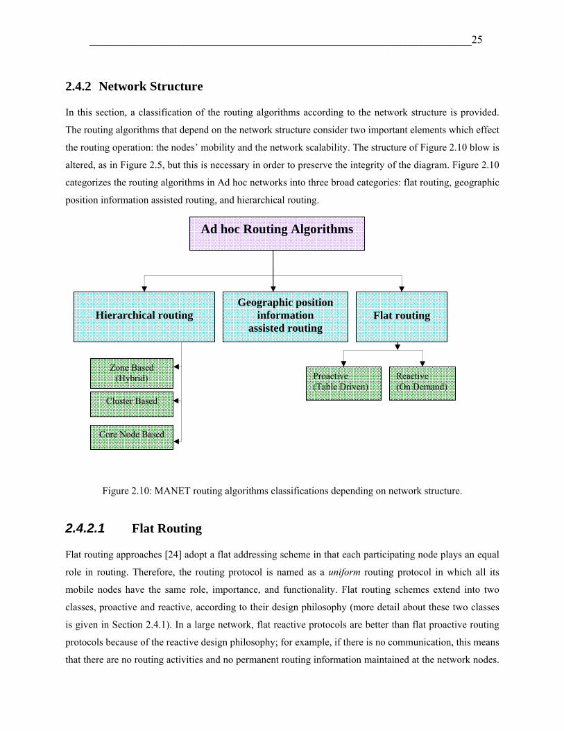
_____________________________________________________________________25
2.4.2 Network Structure
In this section, a classification of the routing algorithms according to the network structure is provided.
The routing algorithms that depend on the network structure consider two important elements which effect
the routing operation: the nodes’ mobility and the network scalability. The structure of Figure 2.10 blow is
altered, as in Figure 2.5, but this is necessary in order to preserve the integrity of the diagram. Figure 2.10
categorizes the routing algorithms in Ad hoc networks into three broad categories: flat routing, geographic
position information assisted routing, and hierarchical routing.
Figure 2.10: MANET routing algorithms classifications depending on network structure.
2.4.2.1 Flat Routing
Flat routing approaches [24] adopt a flat addressing scheme in that each participating node plays an equal
role in routing. Therefore, the routing protocol is named as a uniform routing protocol in which all its
mobile nodes have the same role, importance, and functionality. Flat routing schemes extend into two
classes, proactive and reactive, according to their design philosophy (more detail about these two classes
is given in Section 2.4.1). In a large network, flat reactive protocols are better than flat proactive routing
protocols because of the reactive design philosophy; for example, if there is no communication, this means
that there are no routing activities and no permanent routing information maintained at the network nodes.
Flat routing
Hierarchical routing
Geographic position information
assisted routing
Ad hoc Routing Algorithms
Core Node Based
Cluster Based
Zone Based (Hybrid) Reactive
(On Demand) Proactive (Table Driven)

_____________________________________________________________________26
The Optimised Link State Routing (OLSR) protocol [25], Dynamic Source Routing (DSR) protocol [26]
and Ad hoc On Demand Distance Vector (AODV) routing protocol [27] are examples of uniform routing
protocols.
2.4.2.2 Hierarchical Routing
In contrast to uniform flat routing, non-uniform hierarchical routing usually assigns different roles to
network nodes (as explained in Section 2.4.1.3). Non-uniform routing approaches are related to
hierarchical network structures to facilitate node organization and management. Normally, reactive
algorithms are exploited to select the special nodes which carry out reactive management and/or routing
functions.
In general, flat routing schemes become inefficient when the wireless network size increases due to link
and processing overhead. Therefore, hierarchical routing, as shown in Figure 2.6, has been presented as an
efficient solution to solve the problem and produce a scalable network. As shown in Figure 2.1,
hierarchical routing has been implemented in wired networks for a long time.
Non-uniform hierarchical routing protocols can be further sorted into three subcategories: zone-based,
cluster-based, and core-based. These protocols are categorized according to the organization of the mobile
nodes, their respective management, and their routing functions [5].
A. Zone-based (Hybrid)
Figure 2.9 shows a zone-based hybrid routing algorithm; with this technique, each node has a local scope
and different routing strategies are used, inside and outside the scope, as communications pass across the
overlapping scopes. Given this flexibility, a more efficient overall routing performance can be achieved.
Compared to maintaining routing information for all nodes in the whole network, mobile nodes in the
same zone know how to reach each other with a smaller cost. In some zone-based routing protocols,
specific nodes act as gateway nodes and carry out inter-zone communication. Therefore, the network will
contain partitions or a number of zones. The Zone Routing Protocol (ZRP) [28] is a MANET zone-based
hierarchical routing protocol.
B. Cluster-based
A cluster-based routing protocol is the most popular hierarchical routing technique. It uses a specific
clustering algorithm for cluster head election in which mobile nodes are grouped into clusters by
geographic proximity. Cluster heads then take responsibility on behalf of the cluster for membership

_____________________________________________________________________27
management and routing functions. Cluster head Gateway Switch Routing (CGSR) [29] is an example of a
cluster-based MANET routing protocol. The Hierarchical State Routing (HSR) protocol [30] also supports
a multi-level cluster structure.
C. Core Node-based
In core node-based routing protocols, critical nodes are dynamically selected to compose a "backbone" for
the network. The “backbone” nodes carry out special functions, such as the construction of routing paths
and propagation of control/data packets. Optimised Link State Routing (OLSR) [25] and Core Extraction
Distributed Ad hoc Routing (CEDAR) [31] protocols are typical core node-based MANET routing
protocols.
2.4.2.3 Geographic Position Information Assisted Routing
Routing with assistance from geographic location information requires each node to be equipped with a
Global Positioning System (GPS). This satellite system [32] provides reliable positioning, navigation, and
universal timing services to worldwide users on a continuous basis, in all weather, day and night,
anywhere on Earth. This requirement is quite realistic today since such GPS devices are advanced,
updated, inexpensive, and can provide reasonable precision; GPS provides location information with a
precision within a few meters. Location information can be used for directional routing in distributed Ad
hoc systems. Research in this area has shown that geographical location information can improve routing
performance in Ad hoc networks [33].
Additional care must be taken in a mobile environment because locations may not be accurate by the time
the information is used. All protocols based on GPS assume that the nodes know their positions. The
Location Aided Routing (LAR) [34], the Distance Routing Effect Algorithm for Mobility (DREAM) [35],
and geographical routing [36] are examples of geographic position-assisted routing protocols.
2.4.3 Casting Packets
In this section, the routing algorithms are classified depending on the packet casting type, either unicast or
multicast routing protocols, as shown in Figure 2.11.

_____________________________________________________________________28
Figure 2.11: Routing algorithm classifications depending on packet casting.
There are three categories to cast the control and/or the data packets in network, as shown in Figure 2.12:
a. Unicast: source will send messages to a single destination.
b. Multicast: source will send same messages to specific destinations.
c. Broadcast: source will send same messages to all possible destinations.
Figure 2.12: Packets casting classification.
2.4.3.1 Unicast Routing
Most MANET routing algorithms previously categorized could be classified as unicast routing algorithms
such as Optimised Link State Routing (OLSR) protocols [25], Dynamic Source Routing (DSR) protocols
[26], and Ad hoc On Demand Distance Vector (AODV) routing protocols [27].
(a) Unicast (b) Multicast (c) Broadcast
Mesh based Tree based Group forwarding based
Ad hoc Routing Algorithms
Multicast
Core based
Unicast

_____________________________________________________________________29
2.4.3.2 Multicast Routing
Many multicast routing schemes have been proposed for wired networks, such as the Multicast Open
Shortest Path First (MOSPF) [37] which has been widely used in these networks.
Multicasting in MANET is defined as the transmission of packets to a group of hosts identified by a single
destination address. Multicast service is crucial in management applications where one-to-many
dissemination is necessary. Applications that include close team collaboration in rescue patrols, military
battle, and among scientists with requirements for audio and video communications, are few examples of
multicast routing services.
The classification methods for unicast routing algorithms are also appropriate for the existing multicast
routing algorithms to be classified into reactive, proactive, and hybrid multicast routing. The Ad hoc
Multicast Routing (AMRoute) [38] belongs to the proactive multicast routing category, whereas On
Demand Multicast Routing Protocol (ODMRP) [39] is a reactive multicast routing protocol and the Core-
based Tree (CBT) [40] is a hybrid multicast routing protocol.
Figure 2.11 shows that the existing MANET multicast routing approaches can be subclassified into tree-
based, mesh-based, core-based, and group forwarding-based multicast routing protocols [41]. This
subclassification is based on how the distribution paths among group members are constructed. Some of
the multicast routing protocols could be included in more than one category, such as the Core-assisted
Mesh Protocol (CAMP) [42] which can be characterized as both a core and mesh multicast routing
protocol.
a. Tree-based
In tree-based multicast routing protocols, the source nodes are the roots of multicast trees and in them the
executing algorithm for distribution tree contraction and maintenance. This requires that a source must
know the topology information and address all of its receivers in the multicast group. Therefore, when
used for dynamic networks, source-rooted tree-based multicast routing protocols often suffer from control
traffic overhead. The AMRoute [37] is an example of one such source-rooted tree-based multicast routing.
b. Core-based
In a core-based multicast routing algorithm, cores are nodes with special functions such as multicast data
distribution and membership management. Some core-based multicast routing algorithms also utilise tree
structures, but unlike source-rooted tree-based multicast routing, multicast trees are rooted at core nodes.
For different core-based multicast routing protocols, core nodes may perform various routing and
management functions. For example, in a CBT multicast routing protocol [40], cores are cross points for

_____________________________________________________________________30
all traffic flows of multicast groups and may become bottlenecks along the network. On the other hand, in
protocols like CAMP [42], core nodes are not necessarily utilised by all routing paths.
c. Mesh-based
In a mesh-based multicast routing protocol, packets are distributed along mesh structures that are a set of
interconnected nodes. The mesh structure is more robust than the tree structure for multicast routing in
dynamic networks because a mesh provides alternate paths when link failure occurs. However, the cost for
maintaining mesh structures is normally higher than that of trees. The ODMRP [39] and CAMP [42] are
examples of mesh-based multicast routing protocols.
d. Group Forwarding-based
In the group forwarding-based multicast routing, a set of mobile nodes is dynamically selected as
forwarding nodes for a multicast group. Forwarding nodes then assume the responsibility for multicast
packet distribution. Using this scheme, it is possible to obtain multiple routing paths and send duplicate
messages to receivers through the different paths obtained. ODMRP [39] is a group forwarding-based
multicast routing protocol that uses adaptive forwarding groups to accomplish this.
2.4.3.3 Broadcasting Methods
The broadcasting mechanism is used by MANET nodes for periodic messages (control message). A
number of research groups have proposed efficient broadcast protocols based on distributed and
hierarchical methodologies. The broadcasting methods could be subclassified according to their
transmission methodology, as shown in Figure 2.13. In addition to the simple flooding, the
subclassification includes probability-based methods, area-based methods, and neighbour knowledge
methods. Most existing distributed network-wide broadcast techniques have been summarised and
categorized in Reference [43].
Figure 2.13: Classifications of broadcast methodology.
Area-based Methods
Simple Flooding
Probability-based Methods
Broadcasting Methods
Neighbour Knowledge Methods

_____________________________________________________________________31
a. Simple Flooding
Most of the routing protocols use a generally inefficient form of broadcast called simple flooding. In
simple flooding, when a node receives a packet to be broadcast for the first time, it transmits the packet to
all nodes within its transmission range. In dense networks, the simple flood wastes bandwidth and node
resources. DSR [26] and AODV [27] routing protocols use the simple flooding technique.
The following methods improve upon simple flooding and do not require that every node receive a packet
to transmit it further.
b. Probability-based Methods
Using the probability-based protocols [44], the node decides whether to rebroadcast according to a
specified probability or a simple conditional event which relates to the probability of reaching additional
neighbours.
c. Area-based Methods
Area based methods [44] use knowledge of sender node locations to estimate whether a transmission will
reach a significant amount of additional coverage area. LAR [34] and DREAM [35] include area-based
methods in their routing protocols.
d. Neighbour Knowledge Methods
Neighbour knowledge methods [44] require the use of “Hello”-type packets so that nodes have explicit
data regarding their neighbourhood topology; the nodes then use this neighbour data to decide whether to
rebroadcast a packet. The OLSR routing protocol [25] implements this method.
2.4.4 Network Routing Metrics
In this thesis, a new classification for routing algorithms has been added which depends on the routing
metric. The routing metric used in the identification of the routing path could also be used as a criterion
for MANET routing protocols classification, as shown in Figure 2.14.

_____________________________________________________________________32
Figure 2.14: Routing protocol classifications depending on route metric.
In the previous sections, all mentioned MANET protocols have based on the hop number as a routing
metric, such as in OLSR [25], DSR [26], and AODV [27]. If there are multiple routing paths available, the
path selected will be the shortest routing paths with the minimum hop number in order to decrease traffic
overhead and reduce packet collisions when compared to longer routing paths.
However, one disadvantage to the mobility in MANET is that it can cause route failure and frequently
leads to route discovery. Therefore, the link stability has to be considered in the route construction.
Routing approaches such as Associativity-based Routing (ABR) [45] selects routes based only on nodes’
link stability, where each node has an associative state that implies the period of stability. ABR is a simple
bandwidth-efficient distributed routing protocol that supports mobile computing in a conference-sized
MANET environment. Unlike the proactive or reactive routing algorithms, this protocol does not attempt
to consistently maintain routing information in every node. In this manner, the routes selected are likely to
be long-lived; hence, there is no need to restart frequently, resulting in a higher attainable throughput.
Route requests are broadcast on a per need basis. The protocol is free from loops, deadlock, and packet
duplicates and has scalable memory requirements.
2.5 Summary
This chapter presented a review of the routing process in MANET, which is much more complex than in
wired networks because of the host mobility, interference of wireless signals, and the broadcasting nature
of wireless communication. The complexities of this process and the associated issues have motivated
researchers to develop several MANET routing protocols, with varying performance under different
conditions.
Hop number
Ad hoc Routing Algorithms
Link stability

_____________________________________________________________________33
Each routing protocol developed according to a specific criterion. In this chapter, an overview of four
different MANET routing protocol categories was presented, including design philosophy, network
structure, packets casting, and network routing metric. Each of these categories was used to compare,
classify, and group MANET routing protocols with similar characteristics. These characteristics relate
mainly to the information utilised for routing that determined the nodes’ roles in the routing process. In
this chapter, a new type of classification for MANET routing protocols was added based on network
routing metrics.
The review in this chapter indicates that the invention of new protocols is not a solution due to the large
number of protocols already available. However, there should be an understanding of the network
requirements and conditions for which each protocol is suited and will function best. For each of these
criteria, there is a wide list of protocols that will meet its needs; therefore, this understanding of
requirements and conditions is crucial to selection of the right protocol to enhance efficiency and
performance.
As mentioned previously, focusing on a particular characteristic leads to the design of a particular routing
protocol. Therefore, a range of comparisons between the routing protocols for each criterion should be
made and then evaluated.
2.6 References
[1] J. Andrews, S. Shakkottai, R. Heath, N. Jindal, M. Haenggi, R. Berry, D. Guo, M. Neely, S. Weber,
S. Jafar, and A. Yener, “Rethinking information theory for mobile Ad hoc networks,” IEEE
Communications Magazine, vol. 46, issue 12, pp. 94–101, 2008.
[2] A. S. Tanenbaum, “Computer Networks”, 4th Edition, Prentice Hall PTR, 2003.
[3] J. P. Macker and M. S. Corson, “Mobile Ad hoc networking and the IETF,” Mobile Computing and
Communications Review, vol. 2, no. 4, 2000.
[4] S. Corson and J. Macker, “IETF Mobile Ad hoc Networking (MANET): Routing protocol
performance issues and evaluation considerations,” University of Maryland, Network Working Group,
1999, [online], available on: http://www.ietf.org/rfc/rfc2501.txt, [accessed Jun. 30, 2010].
[5] C. Liu and J. Kaiser “A survey of mobile Ad hoc network routing protocols,” University of Ulm,
Tech. Report Series, no. 2003-08, 2005.
_____________________________________________________________________34
[6] S. Sesay, Z. Yang, and J. He, “A survey on mobile Ad hoc wireless network,” Information
Technology Journal, vol.3, no.2, pp. 168–175, 2004.
[7] C. E. Perkins, “Ad hoc network,” Addison-Wesley, 2001.
[8] “Defense Advanced Research Projects Agency,” DARPA, [Online], available on:
http://www.darpa.mil [accessed Sep. 20, 2010].
[9] J. Jubin and J. D. Tornow, “The DARPA packet radio network protocols,” IEEE Proceedings, vol.
75, issue 1, pp. 21–32, 1987.
[10] “Packet switching,” [online], available on: http://en.wikipedia.org/wiki/Packet-switched [accessed
Jun. 30, 2010].
[11] David A. Beyer, “Accomplishments of the DARPA SURAN Program”, Military Communication
Conference, MILCOM’90, IEEE Conference Record, ’A New Era,’ vol. 2, pp. 855–862, 1990.
[12] “First-of-its-kind Ad Hoc/Sensor Network Testbed,” ece Bradley Department of Electrical &
Computer Engineering, 2005, [online], available on:
http://www.ece.vt.edu/news/fall05/sensornetwork.html, [accessed Jun. 30, 2010].
[13] B. M. Leiner, R. J. Ruth, and A. R. Sastry, “Goals and challenges of the DARPA GloMo Program,”
IEEE Personal Communications, vol. 3, issue 6, pp. 34–43, 1996.
[14] R. Ruppe, “Near Term Digital Radio (NTDR) system,” Proceedings of the IEEE Military
Communications Conference, MILCOM 97s, vol.3, pp. 1282–1287, California, USA, 1997.
[15] “Mobile Ad hoc Networks (MANET),” IETF, [Online], available on:
http://www.ietf.org/dyn/wg/charter/manet-charter.html, [accessed Sep. 20, 2010].
[16] “PCMCIA,” [Online], available on:
http://web.archive.org/web/20080822091330/http://www.pcmcia.org/, [accessed Sep. 20, 2010].
[17] “Bluetooth,” [Online], available on: http://en.wikipedia.org/wiki/Blue_tooth, [accessed Sep. 20,
2010].
[18] D. P. Bertsekas and R. Gallager, “Data networks”, Prentice Hall, 2nd Edition, 1991.
[19] C. Hedrick, “Routing Information Protocol,” RFC 1058, 1988.
[20] E. W. Dijkstra, “A note on two problems in connexion with graphs,” Numerische Mathematik,
vol.1, no.1, pp. 269–271, 1959.
[21] J. Moy, “OSPF version 2,” RFC 2328, 1998.

_____________________________________________________________________35
[22] M. Abolhasan, T. Wysocki, and E. Dutkiewicz, “A review of routing protocols for mobile ad hoc
networks”, Ad Hoc Networks, vol. 2, no. 1, pp. 1–22, 2004.
[23] E. M. Royer and C.-K. Toh, “A review of current routing protocols for Ad hoc mobile wireless
networks,” IEEE Personal Communications, vol. 6, issue 2, pp. 46–55, 1999.
[24] X. Hong, K. Xu, and M. Gerla, “Scalable routing protocols for mobile Ad hoc networks,” IEEE
Network, vol. 16, issue 4, pp.11–21, 2002.
[25] T. Clausen and P. Jacquet, “Optimised Link State Routing Protocol (OLSR)” Project Hipercom,
INRIA, IFTF RFC 3626, 2003.
[26] D. B. Johnson, D. A. Maltz, and Y. Hu, “The Dynamic Source Routing Protocol (DSR) for mobile
Ad hoc networks for IPv4”, IETF RFC 4728, 2007.
[27] C. Perkins, E. Belding-Royer, and S. Das, “Ad hoc On Demand Distance Vector (AODV) Routing,”
IETF RFC 3561, 2003.
[28] Z. J. Haas, M. R. Pearlman, and P. Samar, “The Zone Routing Protocol (ZRP) for Ad Hoc
Networks”, IETF MANET Working Group, 2003.
[29] C. C. Chiang, T. C. Tsai, W. Liu, and M. Gerla, “Routing in clustered multihop, mobile wireless
networks with fading channel,” The Next Millennium, Proceedings of IEEE Singapore International
Conference on Networks, SICON, pp. 197–221, 1997.
[30] G. Pei, M. Gerla, X. Hong, and C. C. Chiang, “A wireless hierarchical routing protocol with group
mobility,” IEEE Wireless Communications and Networking Conference, WCNC ’99, vol.3, pp. 1538–
1542, New Orleans, LA, 1999.
[31] P. Sinha, R. Sivakumar, and V. Bharghaven, “CEDAR: a Core-Extraction Distributed Ad hoc
Routing algorithm,” IEEE Journal on Selected Area in Communication, vol. 17, issue 8, pp. 1454–1465,
1999.
[32] A. Fard, “Global Positioning System (GPS),” [Online], available on: http://www.network-
tutorial.com/global-positioning-system-gps, [accessed Sep. 22, 2010].
[33] X. Du, “QoS routing based on multi-class nodes for mobile ad hoc networks,” Ad Hoc Networks,
vol. 2, issue 3, pp. 241–254, 2004.
[34] Y. B. Ko and N. H. Vaidya, “Location Aid Routing (LAR) in mobile ad hoc networks,”
Proceedings of the 4th ACM/IEEE International Conference on Mobile Computing and Networking,
MobilCom’98, pp. 85–97, 1998.

_____________________________________________________________________36
[35] S. Basagni, I. Chlamtac, V. Syrotiuk, and B. WoodWard, “A Distance Routing Effect Algorithm for
Mobility (DREAM),” Proceedings of the 4th ACM/IEEE International Conference on Mobile Computing
and Networking, MobilCom’98, pp. 76–84, 1998.
[36] R. Jain, A. Puri, and R. Sengupta, “Geographical routing using partial information for wireless Ad
hoc networks,” IEEE Personal Communications, vo. 8, issue 1, pp. 48–57, 2001.
[37] J. Moy, “Multicast Open Shortest Path First (MOSPF),” RFC 1584, 1994.
[38] J. Xie, R. Talpade, A. McAuley, and M. Liu, “AMRoute: Ad hoc Multicast Routing protocol,”
Mobile Networks and Applications vol. 7, no.6, pp. 429–439, 2002.
[39] S. J. Lee, M. Gerla, and C.C. Chiang, “On Demand multicast routing protocol,” Proceedings of
IEEE WCNC’99, pp. 1298–1302, New Orleans, LA, 1999.
[40] A. Ballardie, “Core Based Trees (CBT version 2) multicast routing protocol specification,” Internet
Request for Comment 2189, 1997.
[41] T. Omari, G. Franks, and M. Woodside, “On the effect of traffic model to the performance
evaluation of multicast protocols in MANET,” Canadian Conference on Electrical and Computer
Engineering, pp. 404–407, 2005.
[42] J. J. Garcia-Luna-Aceves and E.L. Madruga, “The core-assisted mesh protocol,” IEEE Journal on
Selected Areas in Communications, vol. 17, issue. 8, pp. 1380–1394, 1999.
[43] B. Williams and T. Camp, “Comparison of broadcasting techniques for mobile Ad hoc networks,”
Proceedings of ACM Symposium on Mobile ad Hoc networking and computing (MobiHoc), pp. 194–205,
2002.
[44] B. Williams, D. P. Mehta, T. Camp, and W. Navidi, “Predictive models to rebroadcast in mobile Ad
hoc networks,” IEEE Transactions on Mobile Computing, vol. 3, no. 3, pp. 295–303, 2004.
[45] C. K. Toh, “Associativity based routing for Ad hoc mobile networks,” Wireless Personal
Communications Journal, vol. 4, no. 2, pp. 103–139, 1997.

_____________________________________________________________________37
Chapter 3
Optimisation in MANET Routing
Protocol
3.1 Introduction
The evolution in mobile applications demands extra attention from the researcher working to optimise
MANET for better service. The optimisation in MANET, however, is more difficult than that of wired
networks due to MANET characteristics such as lack of centralization, network mobility, and multi-hop
communications. Routing optimisation is therefore one of the most important fields in today’s MANET
development.
The main contribution of this chapter will be to present the optimisation work in MANET routing
protocols up to now. Various classifications for the optimised routing protocols have been presented
according to the routing metrics, the prediction techniques, or the use of Artificial Intelligence (AI). The
chapter then identifies the relationship between the works reviewed and the work within the thesis.
The chapter is organised as follows: Section 3.2 includes an overview of the invented MANET optimised
routing protocols based on routing metrics, predictions techniques, and AI techniques; Section 3.3 relates
the work in this thesis to other research reviewed in terms of objectives, models, the prediction method,
and design; and finally, the conclusion is given in Section 3.4.
3.2 MANET Routing Protocol Optimisation
In MANET, optimisation has been used in different wireless layers and in a variety of techniques. The
attention of researchers over the last decade, however, has been focused specifically on enhancing the
MANET routing protocols. The principle behind optimizing MANET route is to control the flows in the
network such that the flows are given better or best-effort treatment. Therefore, the best metrics to
represent the success of the optimisation process and also measure MANET performance could be

_____________________________________________________________________38
increased throughput, reduced packet loss, reduced latency, and reduced load. As such, the literature tends
to focus on throughput and delay as the two most important performance metrics for optimisation
solutions.
3.2.1 Optimum Routing Protocols Based on Routing Metrics
In the literature, most of the optimise protocols, as in [1], are designed based on traditional or widely
implemented protocols. These optimised protocols have been enhanced from the original routing protocols
by including some features that perform the optimisation. This process converts the traditional routing
protocols to an optimise protocol.
MANET optimisation has been based on routing metrics, such as the traditional hop count metric, and the
context-aware metrics, as discussed below.
3.2.1.1 Hop Count Metric
Selecting the optimum path (that with the least cost) according to the hop count metric is one way of
optimizing the route. The optimum route relaying on the minimum hop count could be accomplished in
different ways, such as: by selecting the shortest path (node by node), as in Al-Khwildi and Al-Raweshidy
[2]; by selecting one of many paths discovered through the route discovery process, as in Dai and Wu [3];
or by a unicast query in the route discovery process, as in Seet et al. [4].
3.2.1.2 Context-Aware Metrics
In Ad hoc networks, routing not only has to be fast and efficient, but also adaptive to the changes in the
network topology; otherwise, the performance may be severely degraded. As mentioned before, route
optimisation can be accomplished by considering those context-aware metrics which measure MANET
performance. Context-aware metrics could include mobility awareness, energy awareness, power
awareness, availability, contention awareness, and congestion awareness. Research to find more context-
aware metrics that affect the routing process is ongoing. Including such metrics in the invented protocols
should help to improve MANET performance.
Examples of those context-aware metric(s) that researchers depend upon to create their optimised protocol
are listed below:
1. The energy-aware metric was represented by two objectives; node’s life time and the overall
transmission power were the basis for creating the battery-life aware routing schemes for wireless Ad hoc

_____________________________________________________________________39
networks in [5]. In that development, the aim was to minimize the overall transmission power requested
for each connection and to maximize the lifetime of Ad hoc wireless networks, meaning that the power
consumption rate of each mobile host must be evenly distributed.
The routing schemes invented by Kim et al. [6] also relied on an energy aware context metric to select the
path of least cost and sufficient resources.
Furthermore, in the Mukherjee et al. paper [7] the energy aware metric was the major element in
developing an analytical optimised method to minimize routing energy overhead.
In the multicast routing field, Moh et al. [8] invented a robust two-tree multicast protocol also based on
the energy aware context. This protocol uses two trees, a primary and an alternative backup tree, to
improve the energy efficiency and to offer a better energy balance and packet delivery ratio.
2. The bandwidth-aware metric was utilised to create the Mukhija and Bose [9] Reactive Routing
Protocol.
3. The congestion-aware metric was utilised in the Lu et al. paper [10] to establish distance vector
routing protocol.
In addition, more than one context-aware metric was combined with the routing metric to achieve a better
outcome. Reference [11] introduced the availability aware metric that is represented by the quantity
relationship of link status and mobility aware, as the quantity is required to predict the link status for a
future time period in consideration of mobility.
Next, path congestion and energy usage metrics were combined with the hop count metric in the Cao and
Dahlberg protocol [12] to represent the cost criteria that defines path cost during Route discovery.
Moreover, the routing schemes developed by Chen and Nahrstedt [13] select the network path with the
least cost and sufficient resources to satisfy a certain delay and bandwidth requirement in a dynamic
mobile environment. This protocol combines hop count with energy, latency, and bandwidth-aware
metrics.
Additionally, energy-aware and congestion-aware metrics were both included in the mobile routing
approach of Ivascu et al. [14].
Usually, the ZRP is configured for a particular network through an adjustment of a single parameter: the
routing zone radius. Paper [15] combines mobility-, contention-, and congestion-aware metrics to address
the issue of configuring the ZRP and providing the best performance for a particular network, at any time.

_____________________________________________________________________40
This paper also adds more parameters that affect the performance of the ZRP, including relative node
velocity, node density, network span, and user data activity.
Finally, other combinations were also possible, such as power-aware and mobility-aware metrics for
mobile Personal Area Network in Park et al. [16]. This optimisation technique includes context-aware
metrics with routing metrics that would be effective when activated or employed in an online or real
scenario.
3.2.2 Optimum Routing Protocols Based on Prediction
While the previous optimisation technique based on routing metrics can be considered as one type of
optimizing, another optimisation type is the predication technique. Optimising routing metrics based on
prediction is utilised in networking to achieve a better outcome. Prediction yields an initial idea about the
behaviour of network elements. In the study by Jiang et al. [17], an equation was formulated to predict the
link status for a time period in the future for a mobility aware quantity, whereas Ghosh et al. [18]
predicted the user movement based on GPS receivers to control a hub-based orbital pattern in the
Sociological Orbit aware Location Approximation and Routing (SOLAR) protocol.
3.2.3 Optimum Routing Protocols Based on Modelling /Prediction Techniques
Modelling is another optimisation technique which is also included in the literature. The modelling
process in MANET is utilised to support the prediction technique, as it includes the estimation of various
performance metrics for the multi-hop wireless networks; for example, the empirical model in [19]
developed to characterize the relationship between the proposed response indexes, according to influential
factors. The four response indexes were packet delivery ratio, end-to-end delay, routing overhead, and
jitter. The influential factors were node mobility, offered load, network size, and routing protocol.
A mathematical framework to model contention was presented by Jindal and Psounis [20]. This
framework was used to analyse any routing scheme, with any mobility and channel model. This
framework can also compute the expected delays for different representative mobility-assisted routing
schemes under random direction, random waypoint, and community-based mobility models. This
framework could be considered mobility model aware as it investigated three different mobility models
[21] to conclude the delay. The delay expressions were then used to optimise the design of routing
schemes.

_____________________________________________________________________41
Additionally, in the bi-objective linear programming mathematical area, Guerriero et al. [22] proposed a
bacterium optimisation model which allows the energy consumption and the link stability of mobile nodes
to be taken into account, simultaneously.
Prediction based on modelling is an interesting area in optimisation. This technique was employed by
Nogueira et al. [23] to create a framework to model MANET. The framework integrates important
functional characteristics such as traffic flow, mobility, and background traffic, with each characteristic
represented by its own matrix. The mathematical network model was built from a set of (past) traffic
measurements and the corresponding network performance metrics. This constructed model can then be
used to predict future values of the network metrics, depending on the mathematical cost function, and
based only on the network gateway’s traffic measurements parameters.
3.2.4 Optimum Routing Protocols Based on Application Requirements
Prediction based on MANET application requirements is a very important issue that could be considered
as another type of optimisation in MANET. The Cross-layer Route Discovery Framework (CRDF) [24]
proposes Routing Strategy Automation (RoSAuto) technique that enables wherein each source node
automatically decides the routing strategy based on the application requirements, and then each
intermediate node further adapts the routing strategy so that the network resource usage can be optimised.
In addition, CRDF was designed to provide a flexible architecture for searching desirable routes with low
control overhead. CRDF relies on the Priority-based Route Discovery Strategy (PRDS) mechanism to
solve the “next-hop racing” problem and the “rebroadcast redundancy” problem.
3.2.5 Optimum Routing Protocols Based on Programmable Framework
Prediction based on a programmable platform is another type of optimisation in MANET. Papers [25],
[26], and [27] present a context-based programmable framework and functionality for dynamic
service/protocol deployment. This technique allows the nodes of a MANET to download and safely
activate the required service/protocol software dynamically. According to the available contextual
information, the nodes will evaluate the preconditions that will trigger the downloading and activation.
This strategy leads to the arrangement of the nodes’ capabilities so that common services and protocols
can be deployed even if the downloading and activation are not available at every node. In addition,
dynamic context-driven deployment may lead to a degree of network self-optimisation.

_____________________________________________________________________42
3.2.6 Optimum Routing Protocols Based on Artificial Intelligence
Evolving Artificial Intelligence (AI) has played a key role in optimisation. There are a variety of
optimisation techniques to solve MANET routing problems in AI standard repertoire, examples of which
are given below.
3.2.6.1 Neural Network Approach
Guo and Malakooti [28] present a solution for optimizing the route through employing intelligent use of
the nodes’ past experiences of the network traffic conditions in order to make predictions for future
network traffic conditions based on these experiences. Furthermore, Guo and Malakooti developed a
neural network to predict the mean per-packet one-hop delays. The nodes then used the predicted one-hop
delays to participate in dissemination of routing information.
3.2.6.2 Neuro-Fuzzy Approach
Martinez-Alfaro and Hernandez-Vazquez [29] used an Adaptive Neuro-fuzzy Inference System (ANFIS)
as a predictor. ANFIS is employed inside an Ad hoc hierarchical network to resolve the route error
optimisation problem. The principal problem to resolve was how many nodes the routing protocol can
accept? Given that, the larger the network size, the more performance will suffer. In this Ad hoc
hierarchical network, ANFIS predicts future node mobility to keep the network working at the same level
irrespective of how many nodes join the network.
3.2.6.3 Swarm Intelligence Approach
Many routing protocols draw inspiration from Swarm Intelligence similar to the ant colony adaptive
routing algorithm of Caro et al. [30]. In their study, the authors presented the algorithm as a robust,
decentralized, and self-organised method of routing.
Moreover, Huang et al. [31] investigated a multicast routing protocol which strived to meet the variation
of network topology behaviour (scalability), and satisfy the requirements of specific multimedia traffic,
utilising Particle Swam Optimisation (PSO) in volatile MANET environments.
In the sensors network, Shih [32] evolved PSO to create an energy aware cluster-based routing protocol
that exploits the geographical location information of nodes to assist in network clustering. Also, in the
same Ad hoc sensor network area based on Swarm Intelligence, a robust mobility aware and energy aware

_____________________________________________________________________43
SIMPLE routing protocol [33] was the solution suggested by Yang et al. for the data acquisition problem
found in those networks with mobile sinks.
Furthermore, Rajagopalan and Shen [34] used the Swarm Intelligence mechanisms in Ad hoc networking
with Swarm Intelligence (ANSI) to produce a congestion aware ANSI routing protocol to select next-hops
for both pure and hybrid Ad Hoc networks.
Finally, based on the Swarm Intelligence mechanism, Shen and Rajagopalan [35] created an adaptive
Protocol-Independent Packet Delivery Improvement Service (PIDIS) mechanism to recover lost multicast
packets. The advantage of this mechanism is that the operations of PIDIS do not rely on any underlying
routing protocol and can be incorporated into any Ad hoc multicast routing protocol.
3.3 Related Work
This section will compare the surveyed works with the work proposed in this thesis, namely the
Intelligent-MANET (I-MAN) routing protocols optimisation system. The comparison elements are
models, prediction, objective, and design.
3.3.1 Models
As seen previously, a mathematical equation was utilised in MANET to create models such as those of
Jindal and Psounis [20], Guerriero et al. [22], and Nogueira et al. [23]. Also relevant is an attempt by
Martinez-Alfaro and Hernandez-Vazquez [29] to utilise AI modelling techniques to solve MANET
routing problems. Although there is a similarity between the work in [23] and the thesis in that both
investigations create MANET models, the work in [23] creates mathematical models, whereas the models
for the I-MAN system are created by deploying AI (that’s mean, by implementing neuro-fuzzy (NF)
technique).
The work in [20] and [22] have created models for parameters in the network, whereas the I-MAN 3D
models in this thesis represent the network performance against context parameters. To our knowledge,
there has been no previous MANET modelling done in this format before.
_____________________________________________________________________44
3.3.2 Prediction
Both work, in [23] and this thesis utilised prediction components for optimisation. The work in [23] relies
on mathematical equations whereas the I-MAN routing protocols optimisation system utilises AI by
implementing Particle Swarm Optimisation.
3.3.3 Design
The main difference between most of the mentioned works and the work in this thesis is that previous
researchers are proposing new protocols to be added to the numerous existing routing protocols, as each
protocol is only useful in a certain network context. However, the I-MAN optimisation system proposes
no new protocol; it is a selection approach that deploys the available routing protocols to their best
advantage.
Second, the work in [20] and [35] on the invented model or mechanism could be applied with any network
routing protocol. Both researches are relevant to the re-tuned system in that they are flexible and can be
adapted to changes.
The Programmable Ad Hoc network (PAN) project [27] shares with the I-MAN optimisation system the
basic design idea to select routing protocol depending on contextual information. Nonetheless, the two
approaches differ in several fundamental ways:
1. The PAN project considers network programmability whereas the I-MAN system considers
optimisation techniques to solve MANET routing problems.
2. The PAN project creates context models utilising lightweight Unified Modeling Language (UML)
whereas the I-MAN system creates AI models utilising neuro-fuzzy.
3. The PAN project models represent the network context alone whereas the I-MAN system 3D models
represent the network performance according to the network context (the network history).
4. The hierarchal network of the PAN project consists of three layers, manger head, cluster head, and
cluster node, whereas the I-MAN system network consists two layers, Intelligent node (cluster head) and
network node (cluster node).
5. Although the PAN project and I-MAN system are both mobility aware and scalability aware, these
parameters were implemented in different ways. For the PAN project, the scalability problem is solved by
changing the network topology to a hierarchal approach that consists of three layers so that as the number

_____________________________________________________________________45
of nodes increases, more clusters are added; the I-MAN system, on the other hand, included the scalability
(network size) as the second context parameter.
6. Finally, the work presented in the PAN project was time discrete; there was no graph presenting one
continuous experimental (or simulation) scenario to show the switching of the invented scheme through
time or which routing protocol (AODV or OLSR) was adopted for each period. Also, the cluster nodes
switching adaptation strategy was not clear.
3.3.4 Objective
Most of the previous protocols surveyed have focused on individually improving the number of network
performance parameters and having multiple objectives, except for the work undertaken in paper [19] and
the system in this thesis. The I-MAN approach is significant in that it can better represent a single
objective by combining the network performance parameters in one equation.
3.4 Summary
Creating the optimised routing protocol in MANET was first represented by the protocol that selects the
shortest path. Later, context-aware metrics were considered to develop and optimise the routing protocols.
Prediction, modelling, and AI techniques were also included to support the optimisation.
Researchers have invented optimum routing protocols with the main goal of their design formulated for
particular objectives in the invented protocol. As such, there are already many routing protocols that
equate the most suitable path with the shortest, most reliable, or most self-organised path. Also, there are
the self-management protocols that are composed of self-protecting, self-healing, self-configuring, and
self-optimizing components. Although they have different objectives, each of these protocols reflects their
objective.
For this reason, the search for the most effective routing protocol that provides the optimum path and
satisfies the entirety of objectives still continues, as to our knowledge no routing protocol can handle and
solve all these objectives at once, although there are many protocols which can solve one, two, or maybe
even three of these objectives. Thus, from the survey undertaken in this chapter, it can be concluded that
there is a need for an approach that could deploy the existing algorithms based on the network’s needs.
_____________________________________________________________________46
3.5 References
[1] S. Jiang, Y. Liu, Y. Jiang, and Q. Yin, “Provisioning of adaptability to variable topologies for
routing schemes in MANETs,” IEEE Journal on Selected Areas in Communications, vol. 22, issue 7, pp.
1347–1356, 2004.
[2] A. N. Al-Khwildi and H. S. Al-Raweshidy, “A proficient path selection for wireless Ad hoc routing
protocol,” The 8th International Conference on Advanced Communication Technology, ICACT 2006, vol.
1, pp. 599–604, 2006.
[3] F. Dai and J. Wu, “Proactive route maintenance in wireless Ad hoc networks,” IEEE International
Conference on Communications, ICC 2005, vol. 2, pp. 1236–1240, 2005.
[4] B. Seet, B. Lee, and C. Lau, “Optimisation of route discovery for dynamic source routing in mobile
Ad hoc networks,” IET Journals, Electronics Letters, vol. 39, issue 22 , pp. 1606–1607, 2003.
[5] C. K. Toh, H. Cobb, and D. A. Scout, “Performance evaluation of battery-life aware routing
schemes for wireless Ad hoc networks,” IEEE International Conference on Communication , ICC 2001,
vol. 9, pp. 2824–2829, 2001.
[6] D. Kim, J. J. Garcia-Luna-Aceves, K. Obraczka, J. Cano, and P. Manzoni, “Routing mechanisms for
mobile Ad hoc networks based on the energy drain rate,” IEEE Transactions on Mobile Computing, vol.
2, no. 2, pp.161–173, 2003.
[7] T. Mukherjee, S. K. S. Gupta, and G. Varsamopoulos “Energy optimisation for proactive unicast
route maintenance in MANETs under end-to-end reliability requirements,” Performance Evaluation, vol.
66, pp. 141–157, 2009.
[8] S. Moh, C. Yu, B. Lee, and H. Y. Youn, “Energy efficient and robust multicast protocol for mobile
ad hoc networks,” Proceedings of the Pacific Rim International Symposium on Dependable Computing,
pp.145–152, 2002.
[9] A. Mukhija and R. Bose, "RRP - A bandwidth-efficient routing protocol for mobile Ad hoc
networks," Proceedings of the 2nd International Information and Telecommunication Technologies
Symposium (I2TS 2003), Florianopolis, Brazil, 2003.
[10] Y. Lu, W. Wang, Y. Zhong, and B. Bhargava, “Study of distance vector routing protocols for
mobile Ad hoc networks,” Proceedings of the First IEEE International Conference on Pervasive
Computing and Communications, PerCom 2003, pp.187–194, 2003.

_____________________________________________________________________47
[11] S. Jiang, Y. Liu, Y. Jiang, and Q. Yin, “Provisioning of adaptability to variable topologies for
routing schemes in MANETs,” IEEE Journal on Selected Areas in Communications, vol. 22, issue 7, pp.
1347–1356, 2004.
[12] L. Cao and T. Dahlberg, “Path cost metrics for multi-hop network routing,” Proceedings of the 25th
IEEE International Conference on Performance, Computing, and Communications, IPCCC 2006, pp.7–
22, 2006.
[13] S. Chen and K. Nahrstedt, “Distributed quality-of-service routing in Ad hoc networks,” IEEE
Journal on Selected Areas in Communications, vol.17, no. 8, pp.1488–1505, 1999.
[14] G. I. Ivascu, S. Pierre, and A. Quintero, “QoS routing with traffic distribution in mobile Ad hoc
networks,” Computer Communications, vol. 32, pp. 305–316, 2009.
[15] M. R. Pearlman and Z. J. Haas, “Determining the optimal configuration for the zone routing
protocol,” IEEE Journal on Selected Areas in Communications, vol. 17, issue 8, pp. 1395–1414, 1999.
[16] M. H. Park, C. M. Park, S. H. Kim, S. B. Hong, and J. S. Choi, “A novel routing protocol for
Personal Area Network MObility (PANEMO) environment,” Proceedings of the 6th International
Conference on Advanced Communication Technology, vol. 1, pp.11–14, 2004.
[17] S. Jiang, Y. Liu, Y. Jiang, and Q. Yin, “Provisioning of adaptability to variable topologies for
routing schemes in MANETs,” IEEE Journal on Selected Areas in Communications, vol. 22, no. 7, pp.
1347–1356, 2004.
[18] J. Ghosh, S. J. Philip, and C. Qiao, “Sociological orbit aware location approximation and routing in
MANET,” Ad Hoc Networks, vol. 5, no. 2, pp.189–209, 2007.
[19] I. Ajbar and D. Perkins, “Evaluating mobile Ad hoc networks: A performance index and statistical
model,” IEEE Proceedings Conferences of 16th International Conference on Computer Communications
and Networks, ICCCN 2007, pp. 284–290, 2007.
[20] A. Jindal, and K. Psounis, “Contention-aware performance analysis of mobility-assisted routing,”
IEEE Transactions on Mobile Computing, vol. 8, no. 2, pp.145–161, 2009.
[21] T. Camp, J. Boleng, and V. Davies, “A survey of mobility models for Ad hoc network research,”
Wireless Communication and Mobile Computing, WCMC, Special issue on Mobile Ad Hoc Networking:
Research, Trends and Applications, vol. 2, no. 5, pp. 483–502, 2002.
[22] F. Guerriero , F. De Rango, S. Marano, and E. Bruno, “A biobjective optimisation model for routing
in mobile Ad hoc networks,” Applied Mathematical Modelling , vol. 33, no. 3, pp.1493–1512, 2009.

_____________________________________________________________________48
[23] A. Nogueira, P. Salvador, and R. Valadas, “Joint modeling of MANET characteristics for QoS
prediction,” The 12th IEEE Symposium on Computers and Communications, ISCC 2007, pp. 429–435,
2007.
[24] B. Zhou, A. Marshall, J. Wu, T. H. Lee, and J. Liu, “A cross-layer route discovery framework for
mobile Ad hoc networks,” EURASIP Journal on Wireless Communications and Networking, issue 5, pp.
645–660, 2005.
[25] A. Malatras, G. Pavlou, and S. Sivavakeesar, “A programmable framework for the deployment of
services and protocols in mobile Ad hoc networks,” IEEE Transactions on Network and Service
Management,vol. 4 , issue 3, pp.12–24, 2007.
[26] A. Malatras, A. Hadjiantonis, and G. Pavlou, “Exploiting context-awareness for the autonomic
management of mobile Ad hoc networks,” Journal of Network and Systems Management, Springer, vol.
15, no. 1, pp. 29–55, 2007.
[27] “Programmable Ad hoc Network (PAN) project,” EPSRC, Grant Reference: GR/S02129/01,
[Online], available on: http://personal.ee.surrey.ac.uk/Personal/G.Pavlou/projects/PAN, [accessed on Sep.
19, 2010].
[28] Z. Guo and B. Malakooti, “Delay prediction for intelligent routing in wireless networks using neural
networks,” Proceedings of the 2006 IEEE International Conference on Networking, Sensing and Control,
ICNSC '06, pp. 625–630, 2006.
[29] H. Martinez-Alfaro and M. A. Hernandez-Vazquez, “DSR protocol scalability optimisation in
mobile Ad hoc networks with ANFIS,” IEEE International Conference on Systems, Man and Cybernetics,
vol. 4, pp. 3414–3419, 2003.
[30] G. Di Caro, F. Ducatelle, and L. M. Gambardella, “Swarm Intelligence for routing in mobile ad hoc
networks,” In Proceedings of the 2005 IEEE Swarm Intelligence Symposium, SIS 2005, pp. 76–83, 2005.
[31] C. Huang, Y. Chuang, and K. Hu, “Using particle swam optimisation for QoS in Ad hoc multicast,”
Engineering Applications of Artificial Intelligence, vol. 22, issue 8, pp. 1188–1193, 2009.
[32] T. Shih, “Particle swarm optimisation algorithm for energy-efficient cluster-based sensor
networks,” IEICE Transactions on Fundamentals of Electronics, Communications and Computer
Sciences, vol.E89–A, no.7, pp.1950–1958, 2006.

_____________________________________________________________________49
[33] H. Yang, F. Ye, and B. Sikdar, “A swarm-intelligence-based protocol for data acquisition in
networks with mobile sinks,” IEEE Transactions on Mobile Computing, vol. 7, issue 8, pp. 931–945,
2008.
[34] S. Rajagopalan and C. Shen, “ANSI: A swarm intelligence-based unicast routing protocol for hybrid
ad hoc networks,” Journal of Systems Architecture, vol. 52, issue 8, pp. 485–504, 2006.
[35] C. Shen and S. Rajagopalan, “Protocol-independent multicast packet delivery improvement service
for mobile Ad hoc networks,” Ad Hoc Networks, vol. 5, issue 2, pp. 210–227, 2007.

_____________________________________________________________________50
Chapter 4
I-MAN Design
4.1 Introduction
Wireless networks are designed to provide service to their users at an acceptable level; performance
modelling and evaluation should therefore play a crucial part in the designing and monitoring of those
processes which ensure the successful deployment of a network. As such, network traffic and
characteristics should be analysed and properly controlled to achieve the desired service. Reaching this
design stage in MANET demands specific modelling and design tools.
Therefore, in this thesis the aim has been to design an intelligent system employing Soft Computing [1] to
fulfil the above requirement. The goal of Soft Computing is to construct a new generation of Artificial
Intelligence, known as Computational Intelligence, to develop intelligent machines and to solve non-linear
and mathematically un-modelled system problems. Soft Computing, as such is ultimately a method of
modelling. With this method, an intelligent system could be created by combining intelligent techniques
such as fuzzy logic, neuro-computing, and evolutionary, genetic, and probabilistic computing into one
multidisciplinary system. As a result, the intelligent system should have the ability to learn from those
experiences that will lead to an achievement of the system objectives. In other words, it senses its
environment and learns the correct action for each situation [2].
In this chapter, the Soft Computing goal has been achieved through considering Artificial Intelligence
(AI) techniques and merging them into one system, as the AI system could be a program that has inputs
and learns which outputs get the most approval, either by human beings or a program that can contain the
inputs from the system previous knowledge.
This chapter also outlines the components needed to design an intelligent optimised system, and presents
three routing protocols for study and comparison. The main contribution is the novel design of the
Intelligent-Mobile Ad hoc Network (I-MAN) routing protocols optimisation system.
The remainder of the chapter is organised as follows: in Section 4.2, the I-MAN routing protocols
optimisation system design elements are presented and explained in detail; in Section 4.3, the three

_____________________________________________________________________51
selected routing protocols implemented with the proposed design (the intelligent optimisation system) are
described; with particular focus on the routing protocols’ weaknesses, strengths, and a comparison
between the three protocols; and finally, Section 4.4 includes a chapter summary and findings.
4.2 I-MAN Design Elements
The proposed intelligent system requires contributions from multiple fields, as each field output will
contribute to the proceeding field to create the final intelligent system. The first field is the communication
field, the second is the modelling field, and the third is the optimisation field. The first field is represented
by a wireless MANET whereas the second and the third fields are AI.
The proposed intelligent system objective is to select the optimum routing protocol for MANET, in that
particular context. Therefore, designing the I-MAN routing protocols optimisation system demands
specific simulation, modelling, and optimisation tools. Moreover, different techniques for modelling and
monitoring should be tested in order to create the finest system. Hence, four main components should be
employed, these being the Simulator, Modeller, Optimiser and protocol Switcher (in which the MANET
network will cooperate with the intelligent system to achieve its objective), in conjunction with one
another to accomplish the proposed system’s design,
Given below is a brief list of definitions for all elements needed to create the I-MAN routing protocols
optimisation system.
A. Simulation: simulates MANET in different scenarios containing different contexts, collects the
performance metrics, and then determines the representative value for each performance metric.
B. Modelling: utilises modelling techniques to generate MANET performance models for each
routing protocol depending on entire scenarios.
C. Optimisation: utilises optimisation techniques to optimise MANET performance based on the
performance models by suggesting the optimum routing protocol for the current context.
D. Switching protocols: implements the switching technique between the protocols in MANET and
maintains all the data needing to be transmitted before the switching process in the network.
Figure 4.1 shows the I-MAN routing protocols optimisation system block diagram and the four
aforementioned components. Further explanation of how each component in the I-MAN routing protocols
optimisation system block operates will be given and discussed in detail in the following chapters. Chapter
5 defines the Simulator settings and presents its results; Chapter 6 defines, investigates, and compares the

_____________________________________________________________________52
modelling methods; Chapter 7 defines, investigates, and compares the optimisation techniques employed;
and Chapter 8 explains the modification in the normal wireless node to adopt the protocol switching
technique. This chapter also presents the embedding process for the Modeller and the Optimiser in the
normal wireless node.
The I-MAN routing protocols optimisation system compares and evaluates the protocols and then finds
the best protocol for that context. This proposed system utilised the original and widely implemented
protocols in a similar manner as past researches [3]. The intelligent system includes a list of the evaluated
routing protocols, as more routing protocols could be added or unwanted routing protocols removed from
this list. Each protocol evaluated depended on network performance while the network is operating with a
routing protocol.
Figure 4.1: I-MAN routing protocols optimisation system block diagram.
The arrows in Figure 4.1 represent the system’s task sequences. The yellow arrow represents the
preparation stage, whereas the green arrows represent the case study and implementation process. After
the Simulator finishes its task, its output (represented by the yellow arrow) will be the required input data
for the Modeller.
3. Suggested Routing Protocol
Context & Performance
Simulator
Switcher
Optimiser
Modeller
Implementation process
Preparation process

_____________________________________________________________________53
The system implementation will start from the first green arrow, the current context; will be passed to the
Optimiser. All solutions generated by the Optimiser will then be passed to the Modeller to predict the
network performance for each protocol. The performance metrics will then be calculated and passed to the
Optimiser to select the optimum protocol. The decision to switch to the optimum protocol will then be
passed to the nodes, combined with the threshold time at which the entirety of network nodes will adopt
and operate with this protocol.
The Modeller block represents the models for the previous network performance history. The more data
collected for each model, the more accurate the performance Optimiser’s decision will be. After building
the models for the network performance, the models will act as the Optimiser’s reference. The Optimiser
will refer to the models before its decision.
The flowchart shown in Figure 4.2 lists the intelligent system tasks based on a time scale. The first
preparation procedure simulates the MANET operation with various routing protocols through different
network contexts, then collects and sorts MANET performance parameters. The following procedure
generates the MANET performance models for each operating routing protocol. Then, creating the
intelligent system (that contains the models aforementioned), the system will be activated when it receives
the current MANET context. Next, the system will determine the optimum routing protocol after
optimizing and calculating the network performance as the network operates with each protocol. The
Optimiser optimum protocol will be checked with the routing protocol on operation. If both routing
protocols are the same, then no switching order will be send to the nodes; however, if the protocol is
different, then a switching order will be sent to all the network nodes to switch to the new routing
protocol. This process will be repeated until the simulation is completed.
This intelligent system is responding to the network dynamic changes by continuously updating with the
network context to decide the optimum routing protocol for that period. This means that the network could
benefit from more than one routing protocol throughout the simulation period. Finally, the Optimiser
decision does not rely on a single objective, but on an equation. This equation should include the
performance parameters (objectives) that will help in choosing the optimum routing protocol.

_____________________________________________________________________54
Figure 4.2: Flowchart for the I-MAN routing protocols optimisation system design.
Yes
End of the simulation time?
Optimum selected protocol = Current routing protocol
NoYes
Start
Simulate MANET operations with the routing protocols through different network context and collect MANET performance parameters.
Generate MANET performance models for each operating routing protocol.
(Current MANET context)
Calculate the network performance for each operating protocol.
Switch to the Optimum Routing Protocol.
?
End
No?
Embed the generated models in the intelligent system.
Determine the optimum routing protocol.

_____________________________________________________________________55
4.3 MANET Routing Protocol Techniques
This section contains a description of the MANET routing protocols implemented and evaluated in this
thesis. Three well known and widely implemented routing protocols have been selected for review, the
Optimised Link State Routing (OLSR), Dynamic Source Routing (DSR), and Ad hoc On Demand
Distance Vector (AODV) routing protocols, and are discussed below.
4.3.1 OLSR Routing Protocol
The Optimised Link State Routing (OLSR) protocol [4] is a Table-Driven protocol based on the traditional
Link State algorithm (mentioned in Chapter 2). The point-to-point OLSR routing protocol is a non-
uniform proactive protocol. Under the OLSR routing protocol strategy, nodes in the network exchange
periodical topology information with each other and select a set of neighbouring nodes called MultiPoint
Relays (MPRs) to retransmit their packets. This technique minimizes the size of control messages and the
number of rebroadcast nodes during a route update.
To explain the producer of selecting MPRs [5], Figure 4.3 illustrates how node A selects its MPR set.
Periodic Hello messages will be broadcasted from node A to all immediate neighbours to swap neighbour
lists and calculate the MPR set. Node A deduces from neighbour lists the nodes that are two hops away
and computes the minimum set (MPR set) of one hop relay points vital to reach the two-hop neighbours.
For example, in Figure 4.3, node A selects nodes E, F, and G to be the MPR set. Since the nodes selected
cover all the nodes that are two hops away. Each node notifies its neighbours about its MPR set in the
Hello message. After receiving the Hello message, each node records the selected nodes and calls them
MPR selectors. The frequency of link state updates is adjusted depending on the changes detected in the
MPR set. With a stable MPR set, the period is increased until it reaches a refresh interval value, whereas
with a changing MPR set, the period of link state exchange is set to a minimum value.
Through link state messages, each node obtains network topology information and constructs its routing
table. Routes used in OLSR only include MPRs as intermediate nodes, whereas each node determines, in
terms of hops, an optimal route to every known destination using its topology information (from the
topology table and neighbouring table), and stores this information in a routing table. Therefore, routes to
every destination are immediately available when data transmission begins. Any node which is not MPR
can read and process each packet, but cannot retransmit.

_____________________________________________________________________56
Figure 4.3: An illustration of MPR nodes in the OLSR routing protocol [5].
4.3.2 DSR Routing Protocol Technique
The Dynamic Source Routing (DSR) protocol [6] is a simple On Demand routing protocol for the
purposes of source routing. A reactive routing protocol, DSR allows senders to control the routes used in
routing their packets and also allows multiple routes to any destination. All packets that are sent using
DSR protocol contain the complete list of nodes which the packet will traverse. Each node should
maintain a route cache that includes all known source routes. The route cache will be continually updated
as new routes are learned. When the source’s packets must be sending to some destination, the source first
checks its route cache. If it has an unexpired route to the destination, it will utilise this route to send the
packet, but if the node does not have such a route, it initiates the Route discovery procedure mentioned in
Chapter 2. As shown in Figure 4.4 (a), the source node broadcasts during Route discovery process a route
request packet with a unique identification number. The route request packet encloses the addresses of the
destination and the source nodes. The node that is not the destination node or does not see the same route
request packet as before will attach its IP address to the route request packet and rebroadcast the packet.
Neighbours of node A Nodes E, F, G are A’s MPR Two-hop neighbours of A that are covered by MPR Wireless links Links connecting MPR nodes and the two-hop nodes they covered Links connecting A and its neighbours

_____________________________________________________________________57
The IP Time To Live (TTL) field will be incremented in each Route discovery in order to control the
distribution of the route request packets. The route request packets continue to spread until they reach the
destination node or any other node that has a route to the destination node [7].
Figure 4.4: Formation of Route discovery in DSR.
As shown in Figure 4.4 (b), the destination node responds to the incoming route request packets and
creates a route reply packet that encloses the list of nodes which the route request packet has traversed.
Then, based on a minimal hop count or latency, the source node may select one or more route reply
packets for a single target node.
The DSR Maintenance mechanism consists of the route error packets and the acknowledgments. When
the data link is broken, the node generates these route error packets. Each node that receives a route error
packet removes the hop in error from its route cache and shortens all routes contained by that hop at the
breaking point. In addition to route error messages, the acknowledgments from where the node can hear
the next hop forwarding the packet along the route are useful to verify the correct operation of the route
links [8].
(a) Building of the route record during route discovery
(b) Propagation of the route reply with the route record
DestinationN1
N2
N3
N4
N5
N6
N7
N8
Source
N1-N2-N5-N8
N1-N2-N5-N8
N1-N2-N5-N8
N1
N2
N3
N4
N5
N6
N7
N8
Source
Destination N1 N1-N2
N1 N1-N3
N1-N2-N5
N1-N3-N4
N1-N3-N4
N1-N3-N4
N1-N3-N4-N7
N1-N3-N4-N6
N1-N3-N4-N5
N1-N3-N4-N6-N7

_____________________________________________________________________58
4.3.3 AODV Routing Protocol Technique
The Ad hoc On Demand Distance Vector (AODV) Routing Protocol [9] is a reactive routing protocol
previously mentioned in Chapter 2. AODV borrows the basic Route discovery and the Maintenance
mechanisms from the DSR protocol, whereas AODV borrows the periodic beaconing and the sequence
numbering (the hop-to-hop routing vectors) from the Destination Sequenced Distance Vector (DSDV)
routing protocol [10]. Therefore, the On Demand routing protocol AODV is an optimised distance vector
routing protocol which finds the routes only when required. Also, AODV employs extensively the
sequence numbers in control packets to avoid the problem of routing loops (as explained in the next
section). The AODV protocol is advantageous in that it offers quick adaptation to dynamic link
conditions, low processing, low memory overhead, and low network utilization.
When a source node starts Route discovery to a destination that is not included in its routing table, the
source node broadcasts a route request packet [11], as shown in Figure 4.5 (a). Each route request packet
does contain the following: the ID field that represents a unique identification for the route request packet,
the IP addresses for the source node, the IP addresses for the destination node, the destination sequence
number that specifies the freshness of the control packets, the hop count that maintains the number of
nodes between the source and the destination, and finally, the control flags. The route request starts with a
small TTL value that increases in following route requests when the destination is not found. Each
recipient of the route request packet that has not know the destination IP address or does not maintain a
fresher route to the destination (in another words, does not maintain larger destination sequence number),
rebroadcasts the same packet after monotonically incrementing the hop count. If additional copies of the
same route request are later received, these packets are discarded to reduce overhead. Such intermediate
nodes also create and preserve a reverse route to the source node for a certain interval of time.
When the route request packet reaches the destination node or any node that has a fresher route to the
destination, a route reply packet, as shown in Figure 4.5 (b), is generated and unicast-travelled back to the
source of the route request packet. Each route reply packet contains the destination sequence number, the
IP addresses of the source and the destination, the route lifetime, the hop count, and the control flags. This
guarantees that the route path is being set up bidirectionally. Each intermediate node that receives the
route reply packet, establishes a forward route to the source’s packet, and transmits the packet in it. In
cases where a node receives a new route (by a route request or by a route reply) and it has already a route
‘as fresh’ as the received one, the shortest route will be the one updated.

_____________________________________________________________________59
Figure 4.5: AODV Route discovery.
For the Maintenance mechanism, each node makes use of periodic Hello messages when it needs to detect
link breakages on nodes that it considers as its immediate neighbours. In the case that a link break is
detected for the next hop of an active route, a route error message is sent to its active neighbours using
that particular route. Therefore, the mutable information included in the route error message is the list of
unreachable destinations and their counterparts.
4.3.4 OLSR, DSR, and AODV Loop-Free Technique
The loop problem can be clarified through the following scenario. Assume an existing route link between
A and D, as shown in Figure 4.6; next, the link between S and D, which A is not aware of breaks. For
example, route error message sent by S is lost. Now, assume A wants to send packet to D. It then
performs a route request that can be replied to via path (S-C-A). Node A will reply since it knows a route
to D via node B. This would result in a loop (S-C-A-B-S).
For routing protocols OLSR [4] and AODV [8], an incremental sequence number will avoid the two
protocols having the loops problem in their routing mechanism. Implementing the sequence number
technique in the previous example, the presence of the sequence numbers will let S discover that the
routing information from A is outdated. Node S increments the sequence number when it discovers that
link S-D is broken. In this way, the new sequence number will be greater than the one stored by A.
Source
Destination
(a) Propagation of route request (b) Path of route reply to the source
N1
N2
N3
N4
N5
N6
N7
N8
N1
N2
N3
N4
N5
N6
N7
N8
Source
Destination

_____________________________________________________________________60
Figure 4.6: Loop technique.
On the other hand, DSR [6] provides loop-free routing by requiring path information. DSR establishes a
loop-free route to a destination by carrying the path traversed in route request packets and having the
reverse path piggy-back on (route reply) packets to lead the way to the source, as shown in Figure 4.4 (a
and b). However, given a link failure, reliable error updates must be sent to the source, so that a new route
can be searched.
4.3.5 Comparison of OLSR, DSR, and AODV Routing Protocols
In this section the main strengths and weaknesses of the three routing protocols, OLSR, DSR, and AODV,
have been reviewed. The protocols were evaluated based on the techniques each one used, and their
respective operation conditions.
4.3.5.1 Strengths of OLSR, DSR, and AODV Routing Protocols
Here are some major points that delineate the strengths of each technique and define the best operation
areas for each protocol:
a. OLSR Strengths
OLSR is suited particularly to dense networks. This means that OLSR is not for use in sparse
networks, as all node neighbours become MPR nodes. In this case, the OLSR becomes a pure Link State
protocol and must operate as the original Link State algorithm, such that each node propagates its link
state information to all other nodes in the network [12].
Using the MPR technique minimizes the number of control messages and reduces the message
flooding overhead. OLSR, furthermore, reduces the number of nodes rebroadcasting link state information
(updates). In this way, when a node broadcasts a message, all its neighbours will receive the message and
only the MPR sets will have to forward the link state information [13].
S
A D
C
B

_____________________________________________________________________61
b. DSR Strengths
The DSR protocol offers an acceptable performance and overhead in networks of small to
moderate size. For large networks, however, there will be longer source-destination paths (long route
cache in each node) and an increase in the source path route that piggy-backs on each packet travelling to
its destination [6].
DSR technique nodes can store multiple routes to destinations in their route cache, which means
that there is no need for initiating Route discovery after a breakage if the source node finds a valid route to
the same destination in its route cache [6].
DSR has a satisfying delay since the nodes can store multiple routes in their route cache. The
network nodes delay is the time required to search the node cache for a route before forwarding any data
packets. This is very beneficial in a network with low mobility [14].
DSR does not require any periodic beaconing, or Hello message exchanges. Therefore, nodes can
enter sleep mode to conserve their power and bandwidth [15].
c. AODV Strengths
AODV has two important features which allow the protocol to be adaptable to highly dynamic
networks. First, AODV adopts the destination sequence number technique used by the Destination
Sequenced Distance Vector (DSDV) in an On Demand way. Destination sequence numbers are important
to ensure loop-free and up-to-date routes. Second, AODV maintains in each node a base time state
regarding the utilization of the individual routing table entries, whereas routing table entries will expire if
not recently used [14].
AODV also reduces the flooding overhead. This occurs because AODV routing information is
maintained in the node’s next-hop routing tables containing the destinations for which the node currently
has a route. A routing table entry expires if it has not been used or reactivated for a pre-specified
expiration time. Therefore, the node has only to maintain the routing information about the active paths.
The path, then, will be the result of exchanging the portions of the routing table necessary for establishing
the route [16].
AODV has potentially less routing overheads than DSR, as AODV packets only carry the
destination address ( A route request packet is small in size because it does not contain information about
the whole route path), unlike DSR packets which carry an array of addresses [17].
A node operating AODV MAY offers connectivity information by broadcasting local Hello
messages. A node should only use Hello messages if it is part of an active route. AODV does not require

_____________________________________________________________________62
any periodic beaconing for inactive nodes. Therefore, the inactive nodes can enter sleep mode to conserve
their power and save a considerable amount of bandwidth in the network [18].
4.3.5.2 Weaknesses of OLSR, DSR, and AODV Routing Protocols
This subsection points out the weaknesses of the three routing protocols, as described below:
a. OLSR Weaknesses
OLSR is a Table-Driven protocol that requires periodic beaconing (Hello message exchanges) to
update the network information [15]. These messages will produce an overhead and load the network. The
load will increase if the number of nodes in the network increases. The OLSR routing protocol is unlike
On Demand routing protocols: DSR or AODV, which do not depend on the periodic beaconing in Route
discovery techniques. This also means that OLSR overhead will grow in a network with high mobility
because of the protocol’s frequent topology table update.
b. DSR Weaknesses
DSR is not appropriate for a large network as the overhead may consume most of the bandwidth
[19]. DSR uses source routing that demands every packet should carry the full path address for every hop
in the route from the source to the destination. This means DSR will not be very effective in large
networks as the amount of the path carried in the packet will continue to increase when the network
diameter increases. Also, DSR route replies carry the address of every node along the route [15].
c. AODV Weaknesses
Nodes operating AODV routing protocol may experience large delays during route construction.
Like any On Demand routing protocols, AODV need to establish Route discovery between source and
destination before sending the data packets. Also, if the link failure accrues, Route discovery should be
initiated, which involves extra delays and bandwidth consumption specially when the size of the network
increases [20].
4.3.5.3 Characteristics of OLSR, DSR, and AODV Routing Protocols
Table 4.1 characterizes each of the three protocols in terms of the routing protocol classifications
mentioned in Chapter 2 and the three routing protocol mechanisms mentioned in this chapter.

_____________________________________________________________________63
Table 4.1: OLSR, DSR, and AODV routing protocol characteristics.
OLSR DSR AODV
Routing philosophy Proactive Reactive Reactive
Network structure Hierarchical Flat Flat
Routing metric Hop number
(shortest path)
Hop number
(shortest path)
Hop number
(shortest path)
Broadcasting method Neighbour
knowledge
Simple flood Simple flood
Maintenance Periodically As needed As needed
Periodic Hello message Yes No Yes on need
Use sequence numbers Yes No Yes
Multiple paths No Yes No
Loop free Yes Yes Yes
4.4 Summary
Mobile nodes should not be restricted to operating solely in a particular Ad hoc network context. The
routing scheme should also be able to cope with the performance fluctuation problem. Rather than create
yet another routing protocol to address these issues, this chapter proposes a radical approach to MANET
routing protocols: an Intelligent-Mobile Ad hoc Network (I-MAN) routing protocols optimisation system.
The need for the proposed system arose because degradation of the routing protocol performance is
always associated with the changes in the network context. The I-MAN routing protocols optimization
system abstracting this problem to another level: the environment context is taken into account by a
system that deduces the most appropriate/suitable protocol for the observed conditions. Then, this system,
represented by the Intelligent node, informs the nodes of the routing protocol to run and thus performs
optimally even in the case of continuous changes. In this chapter, a novel I-MAN system design has been

_____________________________________________________________________64
introduced with this simple idea of including various routing protocols in one system and then selecting
the best protocol to operate. I-MAN routing protocols optimisation system design relies on four basic
components: Simulator, Modeller, Optimiser, and Switcher.
The proposed intelligent system acts like an overlay protocol that triggers routing protocols according to
the needs of the network. This system is an attempt to enable a mobile node to achieve its best
performance as it roams through the network, and to provide an automatic routing protocol selection and
adaptation mechanism based on the current topology of the network.
4.5 References
[1] L. A. Zadeh, "Fuzzy logic, neural networks, and soft computing," Communications of the ACM, vol.
37, no. 3, pp. 77–84, 1994.
[2] (E-book) W. Fritz, “Intelligent systems and their societies,” 1997, [online], available on:
http://www.intelligentsystems.com.ar/intsyst, [accessed on Feb. 24, 2010].
[3] S. Jiang, Y. Liu, Y. Jiang, and Q. Yin, “Provisioning of adaptability to variable topologies for
routing schemes in MANETs,” IEEE Journal on Selected Areas in Communications, vol. 22, issue 7, pp.
1347–1356, 2004.
[4] T. Clausen and P. Jacquet, “Optimised Link State Routing protocol (OLSR),” Project Hipercom,
INRIA, IFTF RFC 3626, 2003.
[5] X. Hong, K. Xu, and M. Gerla, “Scalable routing protocols for mobile Ad hoc networks,” IEEE
Network, vol. 16, issue 4, pp. 11–21, Jul.-Aug, 2002.
[6] D. B. Johnson, D. A. Maltz, and Y. Hu, “The Dynamic Source Routing protocol (DSR) for mobile
Ad hoc networks for IPv4”, IETF RFC 4728, 2007.
[7] C. E. Perkins, E. M. Royer, S. R. Das, and M. K. Marina, “Performance comparison of two On
Demand Routing Protocols for Ad Hoc Networks,” IEEE Personal Communications, vol. 8, no. 1, pp. 16–
28, 2001.
[8] R. Duggirala, R. Gupta, Q. Zeng, and D. P. Agrawal, “Performance enhancements of Ad hoc
networks with localized route repair,” IEEE Transactions on Computers, vol. 52, no. 7, pp. 854-861, July,
2003.
_____________________________________________________________________65
[9] C. Perkins, E. Belding-Royer, and S. Das “Ad hoc On Demand Distance Vector (AODV) routing,”
IETF RFC 3561, 2003.
[10] C. E. Perkins and P. Bhagwat, “Highly dynamic Destination-Sequenced Distance-Vector routing
(DSDV) for mobile computers,” Proceedings of the ACM Conference on Communications Architectures,
Protocols and Applications, SIGCOMM '94, pp. 234–244, 1994.
[11] S. Jingfang, W. Muqing, and W. Jingrong; “Comprehensive evaluation of AODV in wireless multi-
hop Ad hoc networks,” The 5th International Conference on Wireless Communications, Networking and
Mobile Computing, WiCom '09, pp. 1–4, 2009.
[12] F. De Rango, J. Cano, M. Fotino, C. Calafate, P. Manzoni, and S. Marano, “OLSR vs DSR: A
comparative analysis of proactive and reactive mechanisms from an energetic point of view in wireless ad
hoc networks,” Computer Communications, vol. 31, issue 16, pp. 3843–3854, 2008.
[13] X. Hong, K. Xu, and M. Gerla, “Scalable routing protocols for mobile Ad hoc networks,” IEEE
Network, vol. 16, issue 4, pp.11–21, 2002.
[14] C. Liu, and J. Kaiser, “A survey of mobile Ad hoc network routing protocols,” University of Ulm,
Tech. Report Series, no. 2003-08, 2005.
[15] H. Pucha, S. M. Das, and Y. C. Hu, “The performance impact of traffic patterns on routing
protocols in mobile Ad hoc networks,” Computer Networks, vol. 51, issue 12, pp. 3595–3616, 2007.
[16] E. M. Royer and C. K. Toh, “A review of current routing protocols for Ad hoc mobile wireless
networks,” IEEE Personal Communications, vol. 6, no. 2, pp. 46–55, April 1999.
[17] M. Abolhasan, T. Wysocki, and E. Dutkiewicz, “A review of routing protocols for mobile Ad hoc
networks,” Ad Hoc Networks, vol. 2, no. 1, pp. 1–22, 2004.
[18] S. Ahmed and M. S. Alam, “Performance evaluation of important Ad hoc network protocols,”
EURASIP Journal on Wireless Communications and Networking, issue 2, pp. 1–11, 2006.
[19] G. Campos and G. Elias, “Performance issues of Ad hoc routing protocols in a network scenario
used for videophone applications,” IEEE Proceedings of the 38th Hawaii International Conference on
System Sciences, pp. 1530–1605, 2005.
[20] L. Layuan, L. Chunlin, and Y. Peiyan, “Performance evaluation and simulations of routing
protocols in Ad hoc networks,” Computer Communications, vol. 30, issue 8, pp. 1890–1898, 2007.
_____________________________________________________________________66
Chapter 5
MANET Simulation
5.1 Introduction
Utilising simulation software packages is beneficial to the testing of any new design. Simulation can save
time, energy, and money as there is no need to order equipment and connect it together to set a scenario.
For example, the OpnetTM14 software package makes it possible to simulate any communication network
for wired or wireless networks in a short time, and the scenario can also provide different services. There
is no doubt about how important it is to establish a test bed for a system to measure its reliability in real
the world, but this step (the test bed) should come after a successful software implementation.
This chapter presents simulations for MANET of different network sizes and average mobility utilising
the OpnetTM14 software package. The main contribution in this chapter is the development of a strategy to
represent the collected MANET performance metrics against the network context. In Section 5.2, the
MANET simulation network will be introduced; this section defines the settings for the communication
model, the movement model, the simulation parameters, and the performance evaluation metrics. The
network simulation results are then presented in 2D and 3D in Section 5.3. Next, Section 5.3.3 analyses
the network results and Section 5.4 summarises the findings of this chapter.
5.2 MANET Simulations
MANET simulations are the first requirement or the first component needed to accomplish the I-MAN
optimisation system design. The network simulations were implemented utilising the OpnetTM14 modeller.
This modeller includes a collection of routing protocols; each routing protocol depends on a different
route discovery mechanism to establish a route to the source destination (as mentioned in Chapter 4). In
this research, a proactive routing protocol (OLSR) and reactive routing protocols (DSR and AODV) were
selected. For each of the three MANET routing protocols, the same MANET simulation environment was
used.
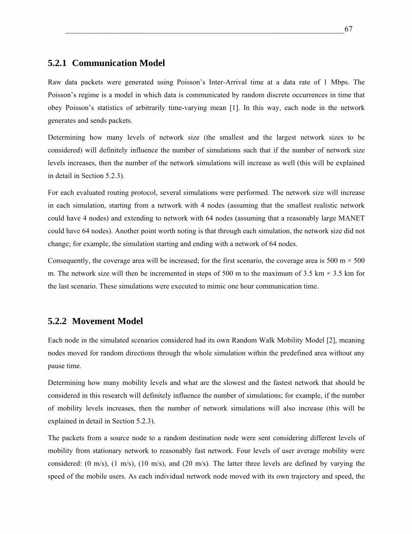
_____________________________________________________________________67
5.2.1 Communication Model
Raw data packets were generated using Poisson’s Inter-Arrival time at a data rate of 1 Mbps. The
Poisson’s regime is a model in which data is communicated by random discrete occurrences in time that
obey Poisson’s statistics of arbitrarily time-varying mean [1]. In this way, each node in the network
generates and sends packets.
Determining how many levels of network size (the smallest and the largest network sizes to be
considered) will definitely influence the number of simulations such that if the number of network size
levels increases, then the number of the network simulations will increase as well (this will be explained
in detail in Section 5.2.3).
For each evaluated routing protocol, several simulations were performed. The network size will increase
in each simulation, starting from a network with 4 nodes (assuming that the smallest realistic network
could have 4 nodes) and extending to network with 64 nodes (assuming that a reasonably large MANET
could have 64 nodes). Another point worth noting is that through each simulation, the network size did not
change; for example, the simulation starting and ending with a network of 64 nodes.
Consequently, the coverage area will be increased; for the first scenario, the coverage area is 500 m × 500
m. The network size will then be incremented in steps of 500 m to the maximum of 3.5 km × 3.5 km for
the last scenario. These simulations were executed to mimic one hour communication time.
5.2.2 Movement Model
Each node in the simulated scenarios considered had its own Random Walk Mobility Model [2], meaning
nodes moved for random directions through the whole simulation within the predefined area without any
pause time.
Determining how many mobility levels and what are the slowest and the fastest network that should be
considered in this research will definitely influence the number of simulations; for example, if the number
of mobility levels increases, then the number of network simulations will also increase (this will be
explained in detail in Section 5.2.3).
The packets from a source node to a random destination node were sent considering different levels of
mobility from stationary network to reasonably fast network. Four levels of user average mobility were
considered: (0 m/s), (1 m/s), (10 m/s), and (20 m/s). The latter three levels are defined by varying the
speed of the mobile users. As each individual network node moved with its own trajectory and speed, the

_____________________________________________________________________68
network nodes’ speed were summed and averaged to determine the network mobility. Therefore, the
mobility levels mentioned previously are the average mobility for the whole network.
5.2.3 Simulation Parameters
The infrastructure-less nature of a MANET, which allows network nodes the freedom to join or leave the
network at any time, will continuously effect the overall network performance. Therefore, this
characteristic could be represented by various parameters [3] such as number of traffic sources, node
bandwidth, node power, node pause time, and all of the parameters mentioned in Chapter 3. In this thesis,
two important context parameters have been considered to evaluate the network performance: the network
size and the nodes’ mobility.
Moreover, the number of simulation scenarios needed for modelling the network depends on two
important elements:
1. The number of selected network context parameters.
2. The number of modelled routing protocols.
The simulation scenarios will increase and decrease depending on these elements, as expressed by
Equation (5.1). Assuming that Pc represents the selected network context parameter, Tc is the total network
context parameters as Tc ≥ 2 and c ≥ 1, and RT is the total number of MANET routing protocols to be
modelled.
Therefore, the total number of the created scenarios ST can be given as:
T
Tc
ccT RPS
c
1 (5.1)
In the I-MAN optimisation system design, the simulations considered two context parameters (PC):
1. Network size level.
2. Mobility level.
Assuming that P1 represents the first parameter that is the network size, Nsize represents the selected
network size, Tsize represents the total number of the network selected cases, and size represents the
selected case, where size ≥ 1, the equation is the following:
Tsizesize
sizesizeNP
11
(5.2)

_____________________________________________________________________69
Assuming that P2 represents the second parameter, namely mobility levels, Mlevel represents the selected
node average mobility level in the network, Tlevel represents the total mobility level cases, and level
represents the mobility level case, where level ≥ 1, then the equation is the following:
levelTlevel
levellevelMP
12
(5.3)
Assuming that Rprotocol, Tprotocol, and protocol represent the MANET routing protocol, the total number of
MANET routing protocol cases used and the protocol number respectively, where protocol ≥ 1 and Tprotocol
≥ 2, then the equation is as follows:
Tprotocolprotocol
protocolprotocolT RR
1
(5.4)
Combining Equations (5.1), (5.2), and (5.3), the equation for the I-MAN simulations scenarios is as
follows:
ST = P1 × P2 × RT (5.5)
In Equation (5.5), the first parameter, P1 mentioned in Equation (5.2), considers seven cases of network
size. Representing various network sizes from small to large, the P1 cases are 4, 9, 16, 25, 36, 49, and 64
nodes, respectively. The second parameter, P2 mentioned in Equation (5.3), has four levels of mobility.
The P2 levels are stationary (0 m/s), low (1 m/s), medium (10 m/s), and high (20 m/s). The last parameter,
RT mentioned in Equation (5.4), considers three routing protocol. From the above it can be determined that
the total number of simulations needed will be 84 (ST = 7 × 4 × 3).
5.2.4 Performance Evaluation Metrics
Through the network simulation, many parameters that present the network performance were collected
and gathered. The correlated parameters were filtered and five important parameters on which to base
network performance selected; these five metrics also reflect the reaction of the other “not selected”
metrics. The performance metrics adopted during the comparative analysis are as follows:
1. Data Drop (bits/s): the total data traffic dropped by the network nodes.
2. Delay (s): the end-to-end packets delay experienced by all nodes.
3. Load (bits/s): the total data traffic received by a all node.

_____________________________________________________________________70
4. Retransmission Attempt (R. A.) (packets): the total number of retransmission attempts by all the
network nodes.
5. Throughput (bits/s): the total number of bits forwarded in all nodes.
5.3 Simulation Results
For each simulation scenario that ran for one hour of simulation time, the results for each respective
metric were recorded and stored. In another words, the simulation network scenario collected the
network’s five performance metrics and presented values every 48 seconds, throughout the simulation
time from the 0s to 3600s. Therefore, the metrics data collected for the five parameters in the 84 scenarios
were stored in 420 data files.
The data collected from all the MANET simulation scenarios should be modelled. Before modelling data,
the data should go through two stages: first, the averaging stage (explained in Section 5.3.1), then the
arranging stage (explained in Section 5.3.2).
5.3.1 Averaging Data
The representative value for each performance parameter should be concluded from the simulation results.
In each scenario, through all the simulation time, the average value for each performance parameter was
calculated. In another words, the mean was computed for the data drop, the delay, the load, the
retransmission attempts (RAs), and the throughput to represent the network performance parameters for
that scenario. Therefore, for each simulation scenario, five performance values were determined. They
were demonstrating the efficiency of the network performance during the one hour of simulation. Figures
5.1 through 5.5 present the averaged five performance metrics: data drop (bits/s), delay (s), load (bits/s),
RAs (packets) and throughput (bits/s). These 2D performance measurers are plotted against network size,
where subfigure (a) represents station network 0 (m/s), (b) relates to the average network mobility 1 (m/s),
(c) relates to the average network mobility 10 (m/s), and (d) relates to the average network mobility 20
(m/s). Each subfigure contains three curves that represents the MANET operated with one of the three
routing protocols OLSR, DSR, or AODV. The parameter network size was labelled as “no. of nodes” in
these graphs.

_____________________________________________________________________71
Figure 5.1: OLSR, DSR, and AODV routing protocols data drop results utilising MANET simulations
with an average mobility a) 0 (m/s), b) 1 (m/s), c) 10 (m/s), and d) 20 (m/s).
Average mobility 10 (m/s)
1
10
100
1000
10000
100000
1000000
0 10 20 30 40 50 60 70
No. of Nodes
Dat
a D
rop
(bit
s/s)
Average mobility 20(m/s)
1
10
100
1000
10000
100000
1000000
0 10 20 30 40 50 60 70
No.of Nodes
Dat
a D
rop
(bit
s/s)
(c) (d)
Average mobility zero (m/s)
0.1
1
10
100
1000
10000
100000
0 10 20 30 40 50 60 70 80
No.of Nodes
Dat
a D
rop
(bit
s/s)
Average mobility 1 (m/s)
1
10
100
1000
10000
100000
0 10 20 30 40 50 60 70No. of Nodes
Dat
a D
rop
(bit
s/s)
(a) (b)
OLSR DSR AODV

_____________________________________________________________________72
Figure 5.2: OLSR, DSR, and AODV routing protocols delay results utilising MANET simulations with an
average mobility a) 0 (m/s), b) 1 (m/s), c) 10 (m/s), and d) 20 (m/s).
Average mobility 10 (m/s)
0.001
0.01
0.1
1
10
100
0 10 20 30 40 50 60 70
No. of Nodes
Del
ay (
s)
Average mobility 20(m/s)
0.001
0.01
0.1
1
10
100
0 10 20 30 40 50 60 70
No. of Nodes
Del
ay (
s)
(c) (d)
Average mobility zero (m/s)
0.001
0.01
0.1
1
10
100
0 10 20 30 40 50 60 70
No.of Nodes
Del
ay (
s)
Average mobility 1 (m/s)
0.001
0.01
0.1
1
10
100
0 10 20 30 40 50 60 70
No. of Nodes
Del
ay (
s)
(a) (b)
OLSR DSR AODV

_____________________________________________________________________73
Figure 5.3: OLSR, DSR, and AODV routing protocols load results utilising MANET simulations with an
average mobility a) 0 (m/s), b) 1 (m/s), c) 10 (m/s), and d) 20 (m/s).
Average mobility 10 (m/s)
0
500000
1000000
1500000
2000000
0 10 20 30 40 50 60 70
No. of Nodes
Lo
ad (
bit
s/s)
Average mobility 20(m/s)
0
200000
400000
600000
800000
1000000
1200000
0 10 20 30 40 50 60 70
No. of Nodes
Lo
ad (
bit
s/s)
(c) (d)
Average mobility zero (m/s)
0
500000
1000000
1500000
2000000
2500000
0 10 20 30 40 50 60 70
No .of Nodes
Lo
ad (
bit
s/s)
Average mobility 1 (m/s)
0
500000
1000000
1500000
2000000
2500000
3000000
0 10 20 30 40 50 60 70
No. of Nodes
Lo
ad (
bit
s/s)
(a) (b)
OLSR DSR AODV
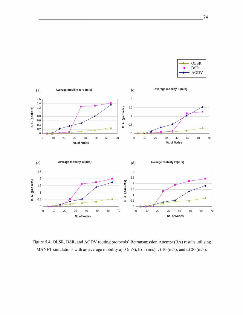
_____________________________________________________________________74
Figure 5.4: OLSR, DSR, and AODV routing protocols’ Retransmission Attempt (RA) results utilising
MANET simulations with an average mobility a) 0 (m/s), b) 1 (m/s), c) 10 (m/s), and d) 20 (m/s).
Average mobility 10(m/s)
0
0.5
1
1.5
2
2.5
0 10 20 30 40 50 60 70
No.of Nodes
R. A
. (p
acke
ts)
Average mobility 20(m/s)
0
0.5
1
1.5
2
2.5
3
0 10 20 30 40 50 60 70
No. of Nodes
R. A
. (p
acke
ts)
(c) (d)
Average mobility zero (m/s)
00.20.4
0.60.8
11.2
1.41.6
0 10 20 30 40 50 60 70
No. of Nodes
R. A
. (p
acke
ts)
Average mobility 1 (m/s)
0
0.5
1
1.5
2
0 10 20 30 40 50 60 70
No. of Nodes
R. A
. (p
acke
ts)
(a) b)
OLSR DSR AODV
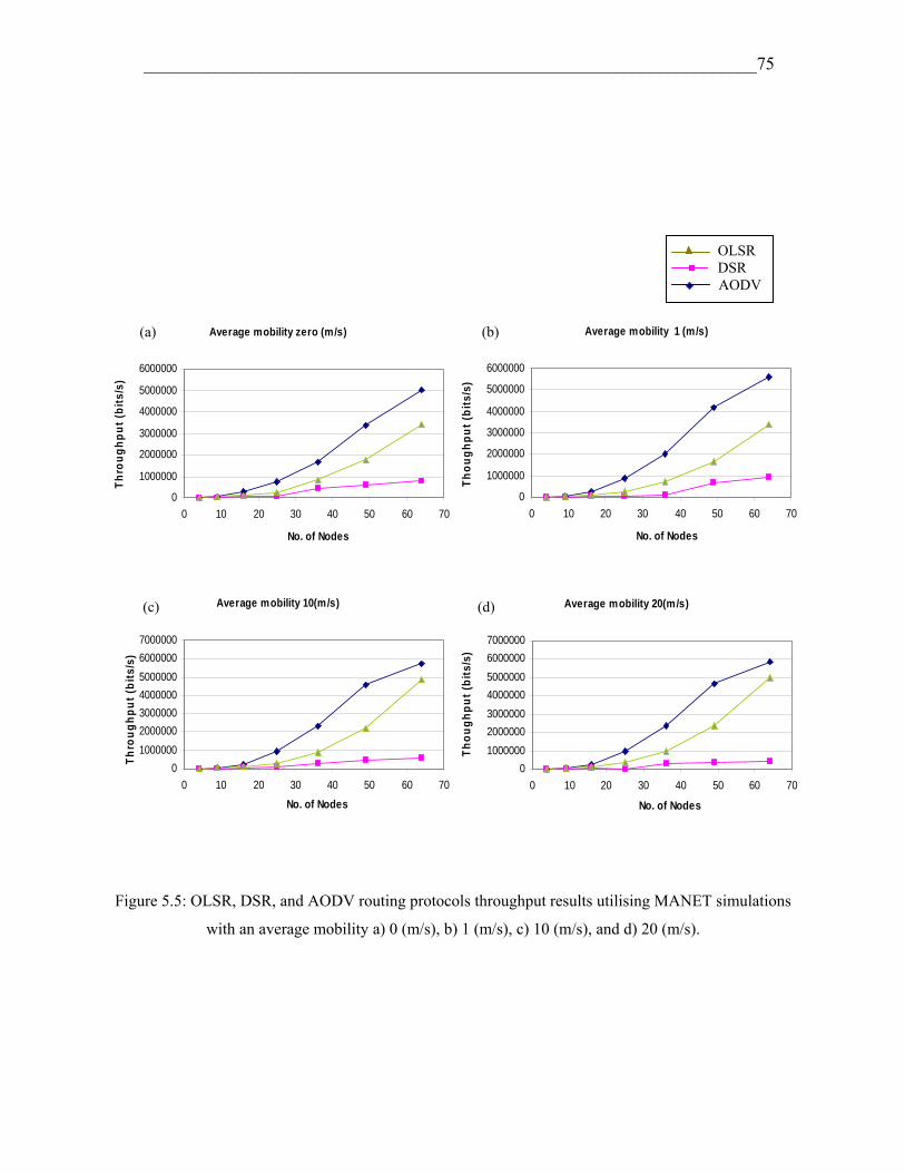
_____________________________________________________________________75
Figure 5.5: OLSR, DSR, and AODV routing protocols throughput results utilising MANET simulations
with an average mobility a) 0 (m/s), b) 1 (m/s), c) 10 (m/s), and d) 20 (m/s).
Average mobility 10(m/s)
0
1000000
2000000
3000000
4000000
5000000
6000000
7000000
0 10 20 30 40 50 60 70
No. of Nodes
Th
rou
gh
pu
t (b
its/
s)
Average mobility 20(m/s)
0
1000000
2000000
3000000
4000000
5000000
6000000
7000000
0 10 20 30 40 50 60 70
No. of Nodes
Th
ou
gh
pu
t (b
its/
s)
(c) (d)
Average mobility zero (m/s)
0
1000000
2000000
3000000
4000000
5000000
6000000
0 10 20 30 40 50 60 70
No. of Nodes
Th
rou
gh
pu
t (b
its/
s)
Average mobility 1 (m/s)
0
1000000
2000000
3000000
4000000
5000000
6000000
0 10 20 30 40 50 60 70
No. of Nodes
Th
ou
gh
pu
t (b
its/
s)
(a) (b)
OLSR DSR AODV
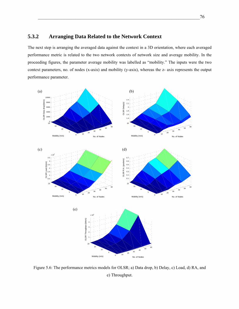
_____________________________________________________________________76
5.3.2 Arranging Data Related to the Network Context
The next step is arranging the averaged data against the context in a 3D orientation, where each averaged
performance metric is related to the two network contexts of network size and average mobility. In the
proceeding figures, the parameter average mobility was labelled as “mobility.” The inputs were the two
context parameters, no. of nodes (x-axis) and mobility (y-axis), whereas the z- axis represents the output
performance parameter.
1020
3040
5060
0
5
10
15
200
2000
4000
6000
8000
10000
No. of NodesMobility (m/s)
OL
SR
Da
ta d
rop
(bits
/s)
1020
3040
5060
0
5
10
15
20
1.4
1.6
1.8
2
2.2
2.4
x 10-3
No. of NodesMobility (m/s)
OL
SR
Del
ay(
s)
1020
3040
5060
0
5
10
15
20
0.5
1
1.5
2
2.5
3
3.5
x 105
No. of NodesMobility (m/s)
OL
SR
Lo
ad (
bits
/s)
1020
3040
5060
0
5
10
15
20
0.1
0.2
0.3
0.4
0.5
0.6
0.7
No. of NodesMobility (m/s)
OL
SR
R.A
. (p
ack
ets
)
1020
3040
5060
0
5
10
15
20
1
2
3
4
x 106
No. of NodesMobility (m/s)
OL
SR
Th
rou
gh
pu
t (b
its/s
)
Figure 5.6: The performance metrics models for OLSR; a) Data drop, b) Delay, c) Load, d) RA, and
e) Throughput.
(a)
(c)
(b)
(d)
(e)

_____________________________________________________________________77
Figures 5.6, 5.7, and 5.8 show the respective performance of OLSR, DSR, and OLSR routing protocols
against the no. of nodes and mobility; the subfigures represent (a) data drop, (b) delay, (c) load, (d) RA.
and (e) throughput.
1020
3040
5060
0
5
10
15
200
2
4
6
8
10
12
x 104
No. of NodesMobility (m/s)
DS
R D
ata
dro
p (
bits
/s)
1020
3040
5060
0
5
10
15
20
5
10
15
20
25
30
35
40
No. of NodesMobility (m/s)
DS
R D
ela
y(s)
1020
3040
5060
0
5
10
15
20
0.5
1
1.5
2
2.5
x 106
No. of NodesMobility (m/s)
DS
R L
oa
d (
bits
/s)
1020
3040
5060
0
5
10
15
20
0.5
1
1.5
2
No. of NodesMobility (m/s)
DS
R R
.A.(
pa
cke
ts)
1020
3040
5060
0
5
10
15
20
0.5
1
1.5
2
2.5
x 106
No. of NodesMobility (m/s)
DS
R T
hro
ug
hp
ut
(bits
/s)
Figure 5.7: The performance metrics models for DSR; a) Data drop, b) Delay, c) Load, d) RA, and
e) Throughput.
(a)
(c)
(b)
(d)
(e)

_____________________________________________________________________78
1020
3040
5060
0
5
10
15
200
1
2
3
4
x 104
No. of NodesMobility (m/s)
AO
DV
Da
ta d
rop
(bits
/s)
1020
3040
5060
0
5
10
15
20
1
2
3
4
5
6
7
No. of NodesMobility (m/s)
AO
DV
De
lay(
s)
1020
3040
5060
0
5
10
15
20
2
4
6
8
10
x 105
No. of NodesMobility (m/s)
AO
DV
Lo
ad
(b
its/s
)
1020
3040
5060
0
5
10
15
20
0.2
0.4
0.6
0.8
1
1.2
1.4
1.6
No. of NodesMobility (m/s)
AO
DV
R.A
.(p
ack
ets
)
1020
3040
5060
0
5
10
15
20
1
2
3
4
5
x 106
No. of NodesMobility (m/s)
AO
DV
Th
roug
hp
ut(b
its/s
)
Figure 5.8: The performance metrics models for AODV; a) Data drop, b) Delay, c) Load, d) RA, and
e) Throughput.
(a)
(c) (d)
(e)
(b)

_____________________________________________________________________79
5.3.3 Results Analysis
In this section the simulation results presented in Figures 5.1 through 5.5 are analysed and discussed
below.
5.3.3.1 Data Drop
In the four subfigures of Figure 5.1, it appears that there is no data drop for the 4-node network size.
Figure 5.1 (a) shows that, in spite of increasing the network size, the least data drop was shown in the
network operating with an OLSR routing protocol. As OLSR is designed to handle scalable networks by
implementing the MPR technique [24], OLSR proactive mechanism also secures in each MPR node a
routing table that contains the routes for all possible destinations. This feature enables OLSR to deliver a
good amount of data without dropping. As shown in the subfigure (a), the station network with 64 nodes
has five-figure number data drop when operated with a DSR routing protocol, whereas utilising OLSR
routing with the same network produced a data drop of only three-figure number.
Figure 5.1 (a) also shows that the DSR routing protocol shows less data drop compared to AODV routing
protocols, for a network size of up to 36 nodes. When a network size is increased to more than 36 nodes,
the routing protocols (AODV and DSR) switch positions and the network implementing AODV routing
protocol achieves less data drop compared to the network that operated with DSR routing protocol. The
reason behind this is that the DSR routing protocol is not designed for a scalable network because of its
route cache mechanism [6]. The side effect of the incremental increase in network size is that the DSR
route cache will also grow. Therefore, the DSR network will suffer from delay increment, as shown in
Figure 5.2 (a), and load increment, Figure 5.3 (a), which will affect the transmission and cause a
significant amount of data drop.
Figure 5.1 (b) shows the different performances for the networks operating with the three protocols. The
network in this figure is dynamic with average mobility (1 m/s). For a network size of up to 36 nodes, the
least data drop is shown with AODV, then DSR, followed by the worst network operating on OLSR. With
a network size of 36 nodes, the best routing protocol is OLSR, followed by DSR, and then AODV;
whereas with a network size of 49 nodes, the best routing protocol is OLSR, followed by AODV, and then
DSR.
In Figure 5.1, (c) and (d) clearly show that for a network size of less than 25 nodes, the least data drop is
for a network which operates on AODV, followed by a network which operates on DSR, and; the worst
results are for a network operating OLSR. With a network size ranging from 25 to up to 49 nodes, the best
routing protocol is AODV, followed by OLSR, and then DSR. With a network size ranging from 49 to up

_____________________________________________________________________80
to 64 nodes, the best routing protocol is OLSR, followed by AODV, and DSR. Furthermore, the results in
Figure 5.1 (c) and (d) show that the AODV routing protocol is efficient for a dynamic network with high
and medium mobility [8].
In Figure 5.1, (a) and (b) when the mobility is low, 0 (m/s) or 1 (m/s), the data started to drop for any
network size greater than 16 (except in the AODV graph which started from 9, as shown in Figure 5.1
(a)); whereas when the mobility is medium, 10 (m/s), or high, 20 (m/s), in Figure 5.1 (c) and (d), the data
started to drop for smaller network sizes, as compared to Figures 5.1 (a) and (b) in which the data started
to drop from any network size greater than 9 nodes. Approximately, the AODV routing protocol was the
only protocol in which the network data drop increased linearly in the log scale by increasing the average
mobility and the network size.
5.3.3.2 Delay
As shown in Figure 5.2 (a), the delay for the networks using AODV and DSR protocols are approximately
the same for a network size of up to 36 nodes. Once this size is exceeded, a rapid increment happens to the
network delay that operates DSR against an acceptable delay for the network that operates AODV, which
will continue through the rest of the simulation. However, the OLSR’s delay is a significant small amount
that does not affected by the network size increase through the simulation compared with the other two
protocols; that is due to OLSR proactive mechanism that stores update table for the whole network and
adopts MPR technique that selects the effective neighbour nodes to retransmit the source packets. As
shown in subfigure (a), a station network of 64 nodes has a delay equivalent to a fraction of a second using
OLSR routing protocol, whereas the same network delay operating DSR reaches a one figure number.
In Figure 5.2 (b), the network is operated with average mobility 1 (m/s); the three routing protocols show
the same attitude as previously seen in Figure 5.2 (a) with a rapid shift in the delay of a network operating
DSR, for a network size of up to 49 nodes.
In Figure 5.2, subfigures (c) and (d) show how medium and high mobility can affect the network delay.
The network operating with DSR showed rapid delay increment for a network size greater than 25 nodes,
whereas the network operate with AODV showed rapid delay increment for network size greater than 49
nodes.
5.3.3.3 Load
Figure 5.3 (a) shows that the stationary networks operating with the three protocols have approximately
the same load until the network size is increased to more than 25 nodes, at which point networks operating
with DSR have the worst load for the duration of the simulation.

_____________________________________________________________________81
In Figure 5.3 (b), when the network’s average mobility is 1 (m/s), the networks operating with OLSR and
DSR have less load than the networks operating with AODV. The load for DSR’s network is clearly better
than the load for the AODV’s network, up to a network size of more than 36 nodes; beyond this point, the
load for DSR’s network suffers rapid increment. This observation is supported by the fact that “the
scalability affects DSR routing protocol” [14].
In Figure 5.3, subfigures (a), (b), (c), and (d) show that the load for the OLSR’s network was significantly
less due to the MPR technique, in spite of the increment in network scalability and mobility, especially in
subfigures (c) and (d). For networks that operate with On Demand protocols, AODV and DSR have higher
load due to the routing establishment mechanism.
5.3.3.4 Retransmission Attempt (RA)
Figure 5.4 shows that the network operating with an OLSR protocol has delivered most of the network
packets. Therefore, the need for RA is less than the other networks operated with AODV and DSR routing
protocols. In a network that operates with a OLSR routing protocol, the node keeps all the neighbouring
nodes’ addresses in the routing table; this characteristic makes it easier for the node to deliver the packets
to their destination. However, networks that operate on the On Demand routing protocols, AODV and
DSR, have to find the destination through establishing a new route if the node does not have the address in
its routing table. For this reason, many packets may not be delivered and will demand another
retransmission attempt.
Figure 5.4 (a) shows that a network operating the DSR routing protocol has less RA than a network that
operates on AODV for a network size of up to 25 nodes, whereas for a network size more than 25 nodes
AODV’s network shows less RA compared to DSR’s network.
In Figure 5.4 (b), the AODV’s and DSR’s network behaviour were similar to their behaviour in Figure 5.4
(a) as DSR’s network has less RA than a network that operates on AODV routing protocol, for a network
size increased to up to 36 nodes. When the network size is 49 nodes, the network operates on AODV has
fewer RA than the DSR network. However, when the network size is 64 nodes, the network operating on
DSR has fewer RA than the AODV network.
Increasing the average mobility, as shown in Figures 5.4 (c) and (d), increases the packets’ retransmission
attempts for a DSR network with a size of 16 nodes. In spite of the increments in the average mobility,
AODV sustains the previous rate of RA which proves the fact that AODV is designed for a dynamic
network [8].

_____________________________________________________________________82
5.3.3.5 Throughput
The four subfigures of Figure 5.5 show that the best throughput was for a network operating with AODV,
followed by a network operating with OLSR, and lastly a network operating with a DSR routing protocol.
The AODV routing protocol was able to forward more packets with the mechanism that quickly
establishes routes and then forwards more packets.
5.4 Summary
Relating the collected MANET performance parameters against the two network context parameters
considered in this thesis and presenting them visually in 3D graphs, this chapter describes a novel,
approach to MANET that has not be explored in previous research. Combining the network contexts in
one graph to present their effects on a particular network performance will dispel the confusion and set a
standard of comparison between the protocols.
This chapter also describes the simulation results for the three MANET protocols AODV, DSR, and
OLSR operating in different scenarios, with multiple network sizes and multiple average mobility (these
results also show the protocols characteristics that having been discussed in Chapter 4). A short summary
and findings for each performance are given below.
The graphs in Figure 5.1 draw a general conclusion that as the mobility increases; the data drop will
increase as well. Also, the figure shows that increasing the mobility affects the data drop for the DSR
operated network more than the ones operated with OLSR and AODV routing protocols, as the DSR data
drop for a network of 64 nodes reached ten four-figure number (bits/s) with average mobility of 20 (m/s).
Figure 5.2 clearly shows that, through the whole simulation for the four subfigures, the best delay is for a
network operating on an OLSR routing protocol, which is related to the MPR mechanism (less message),
The network operating on AODV is second; this may be accounted for by the AODV sequence number
mechanism (drop duplicated messages). The network with the DSR routing protocol is last due to the DSR
cache route mechanism (carry the full path), as the network scalability and mobility affects DSR routing
protocol delay. As shown in subfigure (a), when the network size is 36 nodes, DSR’s delay rapidly
increases. Whereas in subfigures (c) and (d), when the average mobility increases to 10 (m/s) or 20 (m/s),
respectively, the delay for DSR was increased rapidly with network of 25 nodes (smaller that in subfigure
(a)).

_____________________________________________________________________83
In general, Figure 5.3 showed that the load for the networks operated with On Demand protocols were
affected by scalability, especially DSR. As shown in subfigure (a), the networks’ load starts to increase
with a stationary network of 25 nodes and higher. As shown in (b), the loads of networks with average
mobility 1 (m/s), will start to increase with a network size of 36 nodes and higher. When the networks
average mobility is increased to 10 (m/s) and 20 (m/s) respectively, as shown in (c) and (d), the network
will suffer from high load that starts to increase past a network size of 16 nodes. The movement of the
network nodes breaks the early established route, creating a demand for a Route discovery to establish a
new route, which in turn causes load over the network. The load for AODV’s network was less than the
load for DSR’s network the majority of the time; this is related to hop by hop and the sequence number
mechanisms AODV employs. These mechanism will reduce the load by dropping (that is not forwarding)
the packets with old sequence numbers, such that only those packets that have the updated sequence
number will be forwarded.
Also, Figure 5.3 showed that, for the four subfigures through the simulation time, the least load was for
the network that operated on the OLSR routing protocol.
From Figure 5.4, it is clearly shown from the four subfigures that the fewest packets’ retransmission
attempts were accrued for the network that operated on OLSR routing protocol, with the AODV operated
network second and the DSR network third.
Figure 5.5 shows that the best throughput was for a network that operated on AODV, followed by a
network that operated on OLSR, and lastly, a network that operated on DSR.
The results show that OLSR has the best results in terms of delay, load, and retransmission attempts,
whereas AODV has the best throughput. AODV and OLSR perform well with large network sizes and
high mobility, whereas DSR protocol performs at an acceptable level with lower mobility and smaller
network sizes.
The simulation results proved and confirmed that in certain contexts, one of the routing protocols will give
a better performance than the other. However, when the context changes, the first protocol’s performance
will degrade whereas the second protocol’s performance will improve.
5.5 References
[1] I. Bar-David, “Communication under the Poisson regime,” IEEE Transaction of Information
Theory, vol. 15, pp. 31–37, 1969.

_____________________________________________________________________84
[2] T. Camp, J. Boleng, and V. Davies, “A survey of mobility models for Ad hoc network research,”
Wireless Communication and Mobile Computing, WCMC, Special issue on Mobile Ad Hoc Networking:
Research, Trends and Applications, vol. 2, no. 5, pp. 483–502, 2002.
[3] D. D. Perkins, H. D. Hughes, and C. B. Owen, “Factors affecting the performance of Ad hoc
networks,” IEEE International Conference on Communications, ICC 2002, vol. 4, pp. 2048–2052, 2002.
[4] T. Clausen and P. Jacquet, “Optimised Link State Routing protocol (OLSR),” Project Hipercom,
INRIA, IFTF RFC 3626, 2003.
[5] D. B. Johnson, D. A. Maltz, and Y. Hu, “The Dynamic Source Routing protocol (DSR) for mobile
Ad hoc networks for IPv4”, IETF RFC 4728, 2007.
[6] C. Perkins, E. Belding-Royer, and S. Das, “Ad hoc On-Demand Distance Vector (AODV) routing”,
IETF RFC 3561, 2003.
[7] C. Liu and J. Kaiser, “A survey of mobile Ad hoc network routing protocols,” University of Ulm
Tech. Report Series, no. 2003-08, 2005.
[8] C. E. Perkins, E. M. Royer, S. R. Das, and M. K. Marina, “Performance comparison of two On
Demand routing protocols for Ad hoc networks, IEEE Personal Communications, vol. 8, no. 1, pp. 16–28,
2001.

_____________________________________________________________________85
Chapter 6
Modelling Methodology
6.1 Introduction
The model’s chief duty is to provide a simplified view of a complex reality. Therefore, the scientific
model should represent the studied characteristics in a logical way that will yield a realistic view. The aim
of creating this non-mathematical model is to construct a formal system for which reality is the only
interpretation [1].
In this chapter, two modelling techniques are considered: the empirical modelling technique represented
by the regression equation (RE), and the Artificial Intelligence (AI) modelling technique represented by
Artificial Neural Networks (ANN) and Neuro-Fuzzy (NF). As such, there are two main contributions in
this chapter; the first is employing the modelling techniques to create models to represent the MANET’s
context and performance, and the second is comparing and selecting one of these techniques to be used as
the Modeller in I-MAN optimisation system.
The chapter is organised as follows: in Section 6.2, the empirical model is defined and the regression
equation explained as an example of such a model; in Section 6.3, first the Artificial Intelligence
modelling methods are defined and then two artificial intelligent methods, ANN and NF, described and
explained in detail; in Section 6.4, the aforementioned modelling techniques are employed with MANET;
in Section 6.4.4, a comparison between the three created MANET models is presented; and finally,
Section 6.5 includes the summary and relevant conclusions.
6.2 Empirical Modelling
The word empirical in the American Heritage Dictionary [2] denotes information gained by means of
observation, experience, or experiment. Therefore, the empirical relationship will be based solely on
observation rather theory, as an empirical relationship requires only confirmatory data irrespective of a
theoretical basis.

_____________________________________________________________________86
As opposed to analytical modelling, empirical modelling is a popular approach to develop process models
using experimental data, which is commonly welcomed by industries [3]. If a theoretical explanation is
found for what were initially empirical relationships, then the latter are no longer considered empirical.
These empirical relationships are merely approximations. Although in practice they may be so accurate as
to make this distinction otherwise unnoticeable, at other times the relationships may later be found to only
hold under certain specific conditions, reducing them to special cases. The regression equation technique
is a popular empirical technique which will be discussed in the proceeding section.
6.2.1 Regression Equation Models
An empirical relationship will create a mathematical statement and one or more empirical relationships
will form an empirical equation. A regression model can be expressed as a mathematical equation that
characterizes a response metric as a function of the independent factors and a set of parameters. The
predicted performance y for the regression model is given in the form of a polynomial equation. The latter
could be either a linear equation of the first order, or a second order equation with first order interaction,
as in Equation (6.1):
2
1 1 110 i
k
i
k
ij
k
iiijiij
k
iii xxxxy (6.1)
The polynomial equation could also be in the form of a third order equation as shown in (6.2), which is
cubic with second or higher order interaction:
3
11 1
22
1 1 110 i
k
iiiij
k
i
k
ijiiiji
k
i
k
ij
k
iiijiij
k
iii xxxxxxxy (6.2)
where: k is the number of factors; β0 is the mean of y; βi, βij, βii ,βiij, and βiij represent the regression
coefficients; and finally, xi and xj are the factors’ value for network factor Xi where j ≤ k. The advantage of
the regression approach is that it results in a physical equation that can be manipulated to allow for the
capture of both the main and interactive effects among factors.
The regression equation has been involved in predicting MANET performance, as in paper [4] wherein the
regression equation develops a performance index and statistical model that can be used as an objective
measure in the evaluation and comparison of Ad hoc networking protocols. Nogueira et al.[5] also
employed a linear regression equation to build a MANET framework. Moreover, second order polynomial
equations in paper [6] helped to model different MANET connectivity levels.

_____________________________________________________________________87
6.3 Artificial Intelligent Modelling Methods
Modelling plays a very import role in designing an artificial system because in modelling one tries to
uncover what actually happens in the natural system. The artificial models are data driven models; that
means they rely on pre-defined functions and AI to structure the networks models. The artificial models
are not empirical models, as they are not the product of mathematical equations alone.
The model [7] characteristics include:
a. Reproduction of some features of the natural system it is supposed to describe.
b. A formulation that should be consistent with what is known about the considered natural system;
parameters cannot take arbitrary values, the mechanisms and structures of the model must have some
biological plausibility.
c. Testable predictions; ideally all the variables and the parameters should be accessible to experiment.
6.3.1 Artificial Neural Networks Models
Artificial Neural Networks (ANN) are physical cellular networks that are able to acquire, store, and utilise
experimental knowledge [8]. This technique is a computer-based algorithm which is modelled on the
structure and behaviour of the neurons in the human brain.
Artificial neural networks are composed of simple elements operating in parallel. As in nature, the
network function is determined largely by the connections between elements. A neural network can be
trained to perform a particular function by adjusting the values of the connections (weights) between
elements [9]. ANN can be trained to recognize and categorize complex patterns [10].
6.3.1.1 ANN Training Methods
Neural networks are commonly trained such that a particular input guides to a specific target. Therefore,
the network is trained based on a comparison of the network output and the target, until the network
output matches the target. A large number of input/target pairs are needed to train a network. This training
method, called the supervised method, is a popular method. Two other methods, the unsupervised and the
direct design, are also useful for training networks as a network can be obtained without previous training.
Unsupervised networks can be used, for instance, to identify groups of data. Also, certain types of linear

_____________________________________________________________________88
networks and Hopfield networks are examples of such direct design [11]. In summary, there are a variety
of design and learning techniques that enrich the choices available to the user [12].
6.3.1.2 ANN Architecture Types
There are two types [13] for neural network architecture: feed-forward networks or feedback networks.
The feed-forward networks permit signals to travel from the input to the output in only one way, which
means that the output of any layer does not affect that same layer. This architecture is extensively used in
pattern recognition.
The feedback networks can have signals travelling in both directions by introducing loops in the network.
Feedback networks (feed-forwarded back propagation) are very powerful networks and can get extremely
complicated. Feedback networks are dynamic, or in a state of continuous change, until they reach an
equilibrium point. They remain at the equilibrium point until the input changes and a new equilibrium
needs to be found. Feedback architectures are also referred to as interactive or recurrent, although the
latter term is often used to denote feedback connections in single-layer organizations.
6.3.1.3 ANN Layers
In general, an ANN consist of three layers (or groups) of units, wherein a layer of “hidden” units connects
a layer of “input” units to a layer of “output” units [13]. In the input units, the raw information is fed into
the network. The hidden unit is determined by the input units and the weights on the connections between
the input and the hidden units. Finally, the output layer is determined by the hidden units and the weights
between the hidden and output units.
The single-layer network will have one hidden layer, whereas the multi-layer network will have multi-
layer hidden layers. Multiple-layer neural networks are quite powerful; the more neurons in a hidden
layer, the more powerful the network will be. For instance, a network of two layers, in which the first
layer is sigmoid and the second layer is linear, can be trained comparatively well to approximate any
function.
6.3.1.4 ANN Functions
As mentioned previously, the behaviour of ANNs depend on both the weights and the input-output
function (transfer function) that is specified (pre-defined) for the units. Typically, the function considered
is rough approximations and falls into one of three categories [13]:
1. Linear (or ramp) unit: the function output is proportional to the function total weighted input.

_____________________________________________________________________89
2. Threshold unit: the function output is set at one of two levels, depending on whether the total input is
greater or less than the threshold value.
3. Sigmoid unit: the function output varies continuously with the change in the input. A sigmoid
function, such as tanh(x), is not a linear function and shows a greater similarity to real neurons than that of
the linear or threshold units.
In MANET, ANN was useful as a predictor in paper [14]. This network utilised two types of neural
networks, Multi-Layer Perceptron (MLP) network and Radial Basis Function (RBF) network, to predict a
delay scheme for mobile wireless networks. The neural networks based on the nodes’ past experience of
the network traffic conditions predicted the intelligent delay for future network traffic conditions.
6.3.2 Neuro-Fuzzy Models
Jang [15] proposed hybridizing ANN with fuzzy logic [16] to create an Adaptive Network Fuzzy
Inference System (ANFIS) [17]. In another words, ANFIS is a fuzzy inference system implemented in the
framework of adaptive networks. The popular term for this intelligent system is the neuro-fuzzy (NF)
system. This system synergizes the two mentioned techniques by combining the human-like reasoning of
fuzzy systems with the learning capacity and connectionist structure of neural networks. Inspired by
Takagi-Sugeno-Kang (TSK) or the Sugeno accurate modelling approach [18], ANFIS performs the
identification of an input-output mapping in the form of a set of N input-output examples, with a fuzzy
architecture.
The ANFIS architecture has been employed to model non-linear functions, identify nonlinear online
components in a control system, and predict a chaotic time series. The main strength of NF systems [19] is
its universal approximations with the ability to solicit interpretable IF-THEN rules, as the system has the
fuzzy reasoning with the network calculation. The neuro-fuzzy system solved the two conflicting
requirements in fuzzy modelling: interpretability versus accuracy.
In order to model complex nonlinear systems [17], the ANFIS model carries out input space partitioning
that splits the input space into many local regions from which simple local models are employed. The
ANFIS uses fuzzy mfs for splitting each input dimension; the input space is covered by mfs with
overlapping, which means that several local regions can be activated simultaneously by a single input.
Membership functions (mfs) were first introduced in Zadeh’s paper “fuzzy sets” [20].

_____________________________________________________________________90
6.3.2.1 NF System Layers
ANFIS can be demonstrated in a five-layer network structure, as shown in Figure 6.1. It can be described
as a multi-layered feed-forward neural network.
1w
11 fw
2w 22 fw
Figure 6.1: ANFIS architecture [17].
The first layer executes a fuzzification process that includes labelling each input. In the figure above, the
ANFIS structure has two inputs, x and y, where each input considered four labels; A1, A2, B1, and B2.
The most popular function used to transform the input in mf is the Gaussian function, where mf has a bell-
shaped function with maximum value equal to 1 and minimum value equal to 0. Both Equations (6.3) and
(6.4) show implementation of the Gaussian function in Figure 6.1 for two inputs, x and y,
ii
i
dcx
A exmf 2)( 2
)(
(6.3)
i
i
i
dcy
B eymf 2)( 2
)(
(6.4)
where c and d are the mfs' parameters that affected mfs shape; c positions the centre of the peak; and d
controls the width of Gaussian bell.
The second layer in Figure 6.1 executes the fuzzy AND of the antecedent part of the fuzzy rules,
)()( ymfxmfwii BAi , where i = 1, 2 (6.5)
A1
A2
B1
B2
f1
f2
Π
Π
Ν
Ν
∑
x
y
x y
Layer 1 Layer 2 Layer 3 Layer 4 Layer 5
x y
f
w1
w2

_____________________________________________________________________91
The third layer in Figure 6.1 normalizes the membership functions (mfs),
21 ww
ww i
i
, where i = 1, 2 (6.6)
The fourth layer in Figure 6.1 executes the consequent part of the fuzzy rules using the linear function,
yqxpf 111 (6.7)
yqxpf 222 (6.8)
and finally, the last layer in Figure 6.1 computes the output of the fuzzy system by summing up the
outputs of the fourth layer.
2211 fwfwf (6.9)
The ANFIS approximation ability to adopt models will depend on the resolution of the input space
partitioning, which is determined by the number of mfs in ANFIS and the number of layers.
In the MANET literature, NF has been used in optimisation, but to our knowledge, there has heretofore
been no attempt to model MANET parameters with the NF system.
6.4 MANET Models
In this research, data is needed to create the models for a MANET. These data were generated using the
OpnetTM14 Simulator (mentioned in Chapter 4). The data information related to the 3D MANET graphs
was ready to be modelled. The regression equation, ANN, and NF defined in the previous sections were
considered to model MANET; therefore, the data was fed to the three modelling techniques. The network
contexts considered as inputs included no. of nodes and mobility, and the network performance considered
as outputs included data drop, delay, load, RA and throughput.
6.4.1 MANET Regression Models
The Essential Regression software package [21] was implemented to derive the Regression Equation (RE)
models; this package analyzes quantitative data using polynomial and multiple linear regressions in a
straightforward and understandable manner.

_____________________________________________________________________92
Table 6.1 shows five equations that represent the output performance parameters for each routing
protocol. Based on either Equation (6.1) or Equation (6.2) in Section 6.2.1, the MANET regression
equations were either second or third order, where N is the network size and M is the average mobility.
Table 6.1: MANET performance parameters’ regression equations results from operating the routing
protocols OLSR, DSR, and AODV.
The regression equations for OLSR’s data drop, load, RA, and throughput are square equations with
second order interaction, whereas OLSR’s delay regression equation is a cubic equation with second order
interaction. The equations modelled the performance parameters for OLSR, as shown in subfigures (a),
(b), (c), (d), and (e) in Figure 6.2.
OLSR
.8.3445.9871.46858.41687.21185.769143.133961.158510
.000005.01002.500003.000082.0000071.0003.00003.000094.0..
.87.235.06.224.902.842.7041.629.6848
.109.1108.1103.1
1006.81086.5103.21003.800004.000003.0001.0
.06.0096.01.09.23.05.1911.101.59
2222
22622
2222
372828
3926727
2222
NMMNMNMNMNThroughput
NMMNMNMNMNAR
NMMNMNMNMNLoad
MNMMN
NMNMNMNDelay
NMMNMNMNMNDataDrop
DSR
.4.16593.349.216904.30079.6395.458169963.54048.152636
.001.000002.000004.000003.004.0004.0003.031.006.038.0..
.3.45397.136.464.243.135279.155745.31638.991353.654412.3038263
.02.0001.000058.000052.058.008.0057.06.43.15.7
.9.613.467.0186.12.19969.17015.1494.159493.364445.24822
2222
322322
322322
322322
322322
NMMNMNMNMNThroughput
MNMMNNMNMNMNAR
MNMMNNMNMNMNLoad
MNMMNNMNMNMNDelay
MNMMNNMNMNMNDataDrop
AODV
322322
33622
322322
3622322
322322
5.14727.4447.335.307.489818.114304.33959.4215009.924801.683497
.0002.0101.4006.00007.006.0002.008.0..
.04.4001.1376.43.36.10384.788.5803.635435.86561.44688
.1086.60005.00002.000005.0008.0002.0005.0107.0109.0448.0
.4.146.1109.05.07.4559.206.2601.330115.3733.2415
MNMMNNMNMNMNThroughput
MNMNMNAR
MNMMNNMNMNMNLoad
MNMMNNMNMNMNDelay
MNMMNNMNMNMNDataDrop
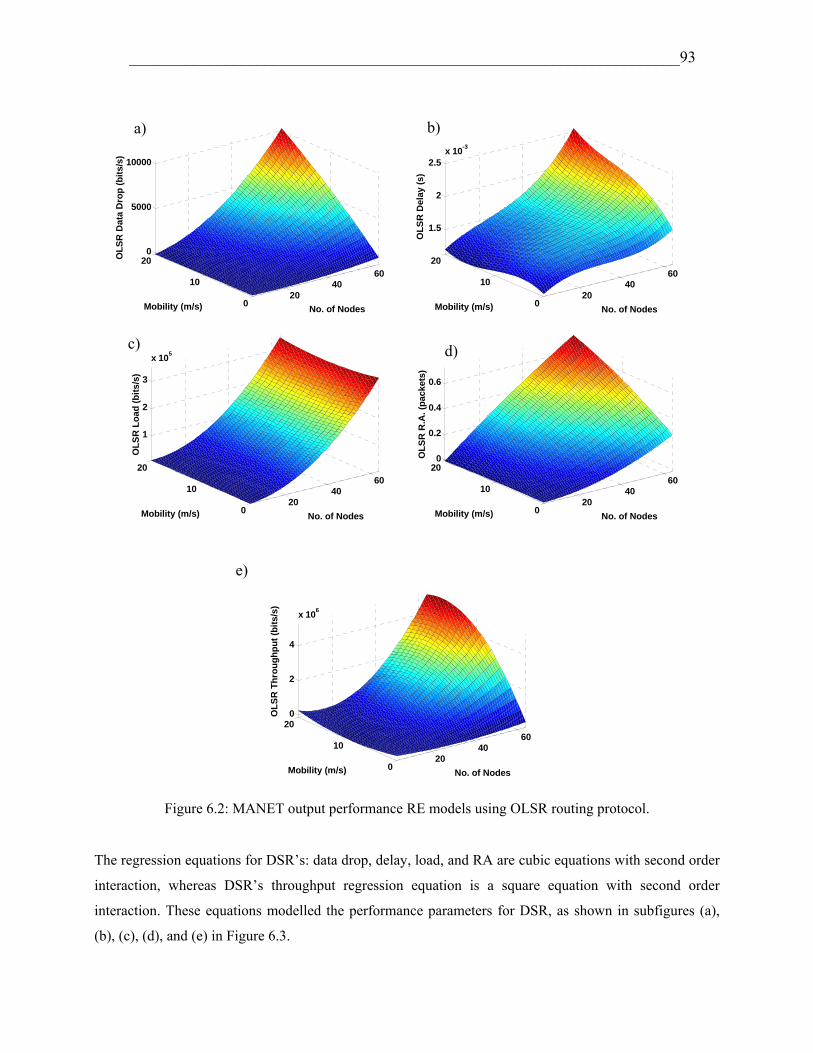
_____________________________________________________________________93
2040
60
0
10
200
5000
10000
No. of NodesMobility (m/s)
OL
SR
Dat
a D
rop
(b
its/
s)
2040
60
0
10
20
1.5
2
2.5x 10
-3
No. of NodesMobility (m/s)
OL
SR
Del
ay (
s)
2040
60
0
10
20
1
2
3
x 105
No. of NodesMobility (m/s)
OL
SR
Lo
ad (
bit
s/s)
2040
60
0
10
200
0.2
0.4
0.6
No. of NodesMobility (m/s)
OL
SR
R.A
. (p
acke
ts)
2040
60
0
10
200
2
4
x 106
No. of NodesMobility (m/s)
OL
SR
Th
rou
gh
pu
t (b
its/
s)
Figure 6.2: MANET output performance RE models using OLSR routing protocol.
The regression equations for DSR’s: data drop, delay, load, and RA are cubic equations with second order
interaction, whereas DSR’s throughput regression equation is a square equation with second order
interaction. These equations modelled the performance parameters for DSR, as shown in subfigures (a),
(b), (c), (d), and (e) in Figure 6.3.
a)
c) d)
b)
e)

_____________________________________________________________________94
2040
60
0
10
20
0
5
10
15x 10
4
No. of NodesMobility (m/s)
DS
R D
ata
Dro
p (
bit
s/s)
2040
60
0
10
20
0
20
40
No. of NodesMobility (m/s)
DS
R D
elay
(s)
2040
60
0
10
20
0
1
2
x 106
No. of NodesMobility (m/s)
DS
R L
oad
(b
its/
s)
2040
60
0
10
20
0
1
2
No. of NodesMobility (m/s)
DS
R R
.A. (
pac
kets
)
2040
60
0
10
200
1
2
x 106
No. of NodesMobility (m/s)
DS
R T
hro
ug
hp
ut
(bit
s/s)
Figure 6.3: MANET output performance RE models using DSR routing protocol.
The regression equations for AODV’s are cubic equations with second order interaction for data drop,
delay, load, and throughput. These equations modelled the performance parameters for AODV, as shown
in subfigures (a), (b), (c), (d), and (e) in Figure 6.4.
e)
c) d)
a) b)

_____________________________________________________________________95
2040
60
0
10
20
0
1
2
3
4
x 104
No. of NodesMobility (m/s)
AO
DV
Dat
a D
rop
(b
its/
s)
2040
60
0
10
20
0
2
4
6
No. of NodesMobility (m/s)
AO
DV
Del
ay (
s)
2040
60
0
10
200
5
10x 10
5
No. of NodesMobility (m/s)
AO
DV
Lo
ad (
bit
s/s)
2040
60
0
10
200
0.5
1
1.5
No. of NodesMobility (m/s)
AO
DV
R.A
. (p
acke
ts)
2040
60
0
10
20
0
2
4
6
x 106
No. of NodesMobility (m/s)
AO
DV
Th
rou
gh
pu
t (b
its/
s)
Figure 6.4: MANET output performance RE models using AODV routing protocol.
6.4.2 ANN MANET Models
MATLABTM was used to program the neural network modular. The ANN modular is constructed as a
feed-forwarded back-propagation network that is composed of three layers: input, hidden, and output, as
illustrated in Figure 6.5.
a)
c) d)
b)
e)

_____________________________________________________________________96
Figure 6.5: ANN MANET model.
The input layer consists of two neurons and the second hidden layer consists of eight neurons, while the
third layer has one neuron. The hidden layer neurons use a hyperbolic tangent sigmoid function to
calculate the layer's output, as shown in Equation (6.10). This transfer function is mathematically
equivalent to the tanh function.
1))2exp(1(2)(
n
nTansig (6.10)
where n is define as
ij
k
jji xwn 1
11
(6.11)
where xj is the input layer to node j; W1ji is the weight between node j in the input layer and node i in the
hidden layer; Ө1i is the bias of node i in the hidden layer (it plays the role of an intercept in the linear
regression); w2i1 is the weight between node i in the hidden layer and the node in the output layer; and Ө21
is the bias of the node in the output layer.
Performance Metrics
Network Context ∑
∑
∑
∑
∑
∑
∑
∑
∑
W2il W1ji
Input layer Output layer
Weights Weights
Hidden layer Өli
Ө21

_____________________________________________________________________97
The output layer corresponds to the performance metric modelled, with a linear transfer function which is
similar to Equations (6.7) and (6.8).
Thus, the predicted performance y given by the neural network model shown in Figure 6.5 could be
expressed as follows:
))(( 21
8
112
nTansigwpureliny
ii
(6.12)
The ANN models were trained to simulate and present the MANET output performance behaviour each
time for one of the three protocols (OLSR, DSR, and AODV). For each routing protocol, five ANN
models were trained. Each model represents one of the five performance parameters against the network
context; training was performed for 10 epochs. In total, 15 models were developed for the three protocols.
A well known fact is that ANNs suffer from overtraining problems as the network incorporates the
inherent “noise” variation of a sample population. As such, MANET models were affected by and suffered
from this problem in the training process. One of the solutions for this problem was the use of the
ensemble modelling technique [22]. This technique was employed with MANET models by training
different neural networks on the same MANET data set. The training generated 10 models in 10 sessions,
with each training session resulting in a different model. After creating the 10 models, the set of the
network context parameter for mobility was partitioned to create 30 values, starting from 0 (m/s) and
ending in 20 (m/s), in the sequence: 0 (m/s), 0.1 (m/s), 0.2 (m/s), 0.3 (m/s),……, 0.9 (m/s), 1 (m/s), 2
(m/s), 3 (m/s),……9 (m/s), 10 (m/s), 11 (m/s), 12(m/s),…… 19 (m/s), and 20 (m/s); next, the new inputs
for the mobility and the network size were entered to the 10 trained neural networks. It is an ensemble of
these 10 models that will be used to create the most dominant MANET, as shown in subfigures (a), (b),
(c), (d), and (e) in Figures 6.6, 6.7, and 6.8.
Comparing the MANET original performance models in Figures 5.6, 5.7, and 5.8 in Chapter 5 with ANN
models, in spite of using the ensemble technique to solve the overtraining problem, some ANN models are
not representative and corrupted. Specifically in Figure 6.7, the models in subfigures (b) and (d) are
corrupted between mobility set 10 and 20, as well as in Figure 6.8 subfigure (b) in which the model is
corrupted between mobility set 20 and 30.

_____________________________________________________________________98
020
4060
80
0
10
20
300
5000
10000
No. of NodesMobility set
OL
SR
Dat
a D
rop
(b
its/
s)
020
4060
80
0
10
20
300
1
2
3
x 105
No. of NodesMobility set
OL
SR
Lo
ad (
bit
s/s)
020
4060
80
0
10
20
30
1.4
1.6
1.8
2
x 10-3
No. of NodesMobility set
OL
SR
Del
ay (
s)
020
4060
80
0
10
20
300
0.2
0.4
0.6
No. of NodesMobility set
OL
SR
R.A
. (p
acke
ts)
020
4060
80
0
10
20
30
0
1
2
3
4
x 106
No. of NodesMobility set
OL
SR
Th
rou
gh
pu
t (b
its/
s)
Figure 6.6: MANET output performance ANN models using OLSR routing protocol.
a)
c) d)
b)
e)

_____________________________________________________________________99
020
4060
80
0
10
20
30
0
2
4
x 105
No. of NodesMobility set
DS
R D
ata
Dro
p (
bit
s/s)
020
4060
80
0
10
20
30
0
20
40
No. of NodesMobility set
DS
R D
elay
(s)
020
4060
80
0
10
20
30
0
5
10
15
20x 10
5
No. of NodesMobility set
DS
R L
oad
(b
its/
s)
020
4060
80
0
10
20
30
0
1
2
No. of NodesMobility set
DS
R R
.A. (
pac
kets
)
020
4060
80
0
10
20
30
0
2
4
6
x 105
No. of NodesMobility set
DS
R T
hro
ug
hp
ut
(bit
s/s)
Figure 6.7: MANET output performance ANN models using DSR routing protocol.
a)
c) d)
b)
e)

_____________________________________________________________________100
020
4060
80
0
10
20
300
1
2
3
4
x 104
No. of NodesMobility set
AO
DV
Dat
a D
rop
(b
its/
s)
020
4060
80
0
10
20
30
0
2
4
6
No. of NodesMobility set
AO
DV
Del
ay (
s)
020
4060
80
0
10
20
30
0
2
4
6
8x 10
5
No. of NodesMobility set
AO
DV
Lo
ad (
bit
s/s)
020
4060
80
0
10
20
300
0.5
1
1.5
No. of NodesMobility set
AO
DV
R.A
. (p
acke
ts)
020
4060
80
0
10
20
30
0
2
4
6x 10
6
No. of NodesMobility set
AO
DV
Th
rou
gh
pu
t (b
its/
s)
Figure 6.8: MANET output performance ANN models through operating AODV routing protocol.
a)
c) d)
b)
e)

_____________________________________________________________________101
6.4.3 NF MANET Models
MATLABTM was utilised to develop MANET neuro-fuzzy models using the Fuzzy Logic Toolbox. All
models were created using the ANFIS package. By using a hybrid learning procedure, ANFIS can
construct an input-output mapping based on both human knowledge (in the form of fuzzy if-then rules)
and stipulated input-output data pairs.
The model topology was based on the TSK type; two Gaussian membership functions for the two input
variables. Depending on the data provided by the MANET Simulator, membership functions (mfs) and
fuzzy rules are established to create 110 NF rules for the output parameters of the three protocols, as
shown in Table 6.2.
Table 6.2: Performance’s neuro-fuzzy membership functions and the three protocols’ fuzzy rules.
Routing
Protocol
Linguistic
Labels
Data
Drop
Retransmission
Attempt
Throughput Delay Load
mf1 × mf2 3×2 3×2 3×3 3×2 3×3 OLSR
rules 6 6 9 6 9
mf1 × mf2 2×2 2×2 2×2 2×2 2×2 DSR
rules 4 4 4 4 4
mf1 × mf2 3×3 4×3 4×3 3×3 4×3 AODV
rules 9 12 12 9 12
If the output performance data suffers rapid changes, this will demand an increase in the number of
membership functions. In contrast, if the performance data has smooth changes, the membership functions
are needed less. In another words, when the number of membership functions increase, the rapid changes
that occur in the model will be clearly reflected.

_____________________________________________________________________102
The number of rules will be affected too, as it is the product of multiplying the membership functions
(mfs) of the input parameters as presented in Equation (6.5). Therefore, the increase in the mfs will also
lead to an increase in the rules. For example, referring to Table 6.2, the AODV load model requires (4 mfs
× 3 mfs). Accordingly, 12 fuzzy rules should be considered for the AODV load model, since the number
of rules depends on the number of mfs. In contrast, all DSR performance models require (2 mfs × 2 mfs),
which produce 4 fuzzy rules.
The rules and the weight for each input parameter will determine the final output model for each protocol
performance, with each model represented by its own number of rules. The training was performed for
three epochs. The MANET NF model’s structures are the same as in Figure 6.1, the only difference is that
MANET inputs parameters: A (no. of nodes) and B (mobility) not always converted into two objects, as
they will converted to more than two objectives. Equations from (6.3) through (6.8) are implemented to
create the NF model for each output performance parameter. For each routing protocol, five NF models
were trained. In total, 15 models were developed for the three protocols.
The 3D shapes shown in subfigures (a), (b), (c), (d), and (e) in Figures 6.9, 6.10, and 6.11 present the NF
models for each routing protocol. The models show how each protocol parameter responds with respect to
the two context parameters as each subfigure represents data for a particular protocol performance. For
example, subgroup figure (a) in Figure 6.11 represents AODV delay response relating to a mobility range
of 0 to 20 (m/s) and network size varying between 4 and 64 nodes.

_____________________________________________________________________103
2040
60
0
10
200
5000
10000
No. of NodesMobility (m/s)
OL
SR
Dat
adro
p (
bit
s/s)
2040
60
0
10
20
1.5
2
2.5
x 10-3
No. of NodesMobility (m/s)
OL
SR
Del
ay(s
)
2040
60
0
10
20
1
2
3
x 105
No. of NodesMobility (m/s)
OL
SR
Lo
ad (
bit
s/s)
2040
60
0
10
200
0.2
0.4
0.6
No. of NodesMobility (m/s)
OL
SR
R.A
. (p
acke
ts)
2040
60
0
10
200
2
4
x 106
No. of NodesMobility (m/s)
OL
SR
Th
rou
gh
pu
t (b
its/
s)
Figure 6.9: MANET output performance NF models using OLSR routing protocol.
a)
c) d)
b)
e)

_____________________________________________________________________104
2040
60
0
10
20
0
5
10
15
x 104
No. of NodesMobility (m/s)
DS
R D
atad
rop
(b
its/
s)
2040
60
0
10
20
0
20
40
No. of NodesMobility (m/s)
DS
R D
elay
(s)
2040
60
0
10
20
0
1
2
x 106
No. of NodesMobility (m/s)
DS
R L
oad
(b
its/
s)
2040
60
0
10
20
0
1
2
x 106
No. of NodesMobility (m/s)
DS
R T
hro
ug
hp
ut
(bit
s/s)
2040
60
0
10
20
0
1
2
3
No. of NodesMobility (m/s)
DS
R R
.A. (
pac
kets
)
Figure 6.10: MANET output performance NF models using DSR routing protocol.
a)
c) d)
b)
e)

_____________________________________________________________________105
2040
60
0
10
200
2
4
6
x 104
No. of NodesMobility (m/s)
AO
DV
Dat
adro
p (
bit
s/s)
2040
60
0
10
200
2
4
6
No. of NodesMobility (m/s)
AO
DV
Del
ay (
s)
2040
60
0
10
20
2
4
6
8
10x 10
5
No. of NodesMobility (m/s)
AO
DV
Lo
ad (
bit
s/s)
2040
60
0
10
200
0.5
1
1.5
2
No. of NodesMobility (m/s)
AO
DV
R.A
. (p
acke
ts)
2040
60
0
10
200
2
4
6x 10
6
No. of NodesMobility (m/s)
AO
DV
Th
rou
gh
pu
t (b
its/
s)
Figure 6.11: MANET output performance NF models using AODV routing protocol.
a)
c) d)
b)
e)

_____________________________________________________________________106
6.4.4 MANET Models Comparison
MANET performance models are very useful for prediction purposes and are helpful in the decision
making process; the Optimiser proposed by this thesis will therefore rely on these models to predict the
output performance for the system and then decide the optimum protocol. As such, the more accurate the
models are, the more accurate the prediction obtained by the decision making process.
Therefore the results of the three different techniques: RE, ANN, and NF, respectively, and the MANET
performance models in Figures 6.2 through 6.11 should be compared to first determine the best models
and then select the best MANET modelling technique.
The regression models, in spite of having second and third order equations, fail to interpret the changes in
the performance data in a representative curvy model, whereas AI (ANN or NF) models represent
MANET performance more realistically. Comparing the AI models together, NF models are smoother,
more efficient, and more accurate than ANN. To present a MANET parameter, ANN models bend and
curve more than NF models through their training epochs (the overtraining problem corrupted the ANN
models).
A quantitative analysis was performed to choose the best representative MANET models. For each output
performance parameter, the Root Mean Square Error (RMSE) of the actual data (Doriginal) and the model
data (Dmodel) was calculated, as defined in Equation (6.13):
n
DDRMSE
n
iioriginalModel
1
2)( (6.13)
Tables 6.3, 6.4, and 6.5 present RMSE calculation results utilising RE, ANN, and NF for MANET
employing OLSR, DSR, and ADOV routing protocols, respectively. For the four performance outputs
delay, load, RA, and throughput, the RMSE of the NF models was the best. The conclusion drawn from
the tables’ results is that the NF models best represent MANET performance and therefore NF models will
be helpful to the proposed system Optimiser.

_____________________________________________________________________107
Table 6.3: Root Mean Square Error for MANET output parameters utilising OLSR routing protocol.
OLSR
RMSE RE ANN NF
Data Drop(bits/s) 161 35 31
Delay (s) 0.0000309 0.0000998 0.0000109
Load (bits/s) 6420 6540 1650
RA (packets) 0.0145 0.008 0.0034628
Throughput (bits/s) 185000 6530 246000
Table 6.4: Root Mean Square Error for MANET output parameters utilising DSR routing protocol.
DSR
RMSE RE ANN NF
Data Drop(bits/s) 10200 7400 1890
Delay (s) 3.5906 3.4121 0.82681621
Load (bits/s) 215000 211000 195000
RA (packets) 0.1988 0.1831 0.03094911
Throughput (bits/s) 242000 192000 55200

_____________________________________________________________________108
Table 6.5: Root Mean Square Error for MANET output parameters utilising AODV routing protocol.
AODV
RMSE RE ANN NF
Data Drop(bits/s) 2230 392 147
Delay (s) 0.3657 0.032 0.01020036
Load (bits/s) 17900 36200 1870
RA (packets) 0.1094 0.4414 0.00843813
Throughput (bits/s) 207000 250000 1270
6.5 Summary
The models created in this chapter employed two modelling approaches. The empirical approach was
represented by regression equations and the AI approach was represented by artificial neural networks
(ANN) and neuro-fuzzy (NF) networks. The models characterize each routing protocol, as each model
represents the protocol’s output parameter response and was trained to represent the network history, as
well as predict the network performance behaviour for any network size from 4 to up to 64 nodes, and an
average mobility from 0 (m/s) to up to 20 (m/s) (not merely the 7 levels of network size and the 4 levels of
average mobility considered in Chapter 5).
In this chapter, a quantitative comparison of the MANET models created by the three modelling
approaches (RE, ANN, and NF) was also undertaken to evaluate each model. This led to the conclusion
that the NF technique is the best technique to represent MANET performance models that support the
decision to choose the optimum routing protocol.
_____________________________________________________________________109
6.6 References
[1] H. Freudenthal, “The concept and the role of the model in mathematics and natural and social
sciences,” pp. 8-9, D. Reidel Publishing Company, Netherlands, 1961.
[2] “The American heritage dictionary of the English language,” 4th Edition. Houghton Mifflin
Company, 2000.
[3] The University of Washington training guide, “Flexible-Empirical method,” Interactive Training
Guides, 2005 [Online], available on: http://training.ce.washington.edu/WSDOT/Modules/
06_structural_design/06-3_body.htm#computer_program, University of Washington, [accessed on Jul. 1,
2010].
[4] I. Ajbar and D. Perkins, “Evaluating mobile Ad hoc networks: A performance index and statistical
model,” Proceedings of 16th IEEE International Conference on Computer Communications and
Networks, ICCCN 2007, pp. 284–290, 2007.
[5] A. Nogueira, P. Salvador, and R. Valadas, “Joint modeling of MANET characteristics for QoS
prediction,” The 12th IEEE Symposium on Computers and Communications, ISCC 2007, pp. 429–435,
2007.
[6] W. Chung and K. Yao; “Empirical connectivity for mobile Ad hoc networks under square and
rectangular covering scenarios,” 2006 IEEE International Conferences on Communications, Circuits and
Systems Proceedings, vol. 3, pp. 1482–1486, 2006.
[7] E. Bonabeau, M. Dorigo, and G. Theraulaz, “Swarm Intelligence from natural to artificial systems”,
Oxford University Press, United States of America, 1999.
[8] K. Gurney, “An introduction to neural networks,” UCL Press, 1997.
[9] J. M. Zurada, “Introduction to artificial neural systems”, West Publishing Company, U.S.A, 1992.
[10] C. M. Bishop, “Neural networks for pattern recognition”, Clarendon Press, Oxford, 1995.
[11] J. Bamunusinghe and D. Alahakoon, “Concept learning from visual experiences using unsupervised
neural networks,” IEEE Third International Conference on Information and Automation for Sustainability,
ICIAFS 2007, pp. 46–51, 2007.
[12] Neural network toolbox™ 6 user's guide,” [Online], available on: www.mathworks.com, [accessed
on Jul. 4, 2010].

_____________________________________________________________________110
[13] C. Stergiou and D. Siganos, “Neural networks,” final report, Surpise 96 Journal, Imperial College
London Department of computing, vol. 4, [Online], available on:
http://www.doc.ic.ac.uk/~nd/surprise_96/journal/vol4/cs11/report.html# Introduction%
20to%20neural%20networks, [accessed on Jul. 4, 2010].
[14] Z. Guo and B. Malakooti, “Delay prediction for intelligent routing in wireless networks using neural
networks,” Proceedings of the 2006 IEEE International Conference on Networking, Sensing and Control,
ICNSC '06, pp. 625–630, 2006.
[15] J. R Jang, “Neuro-fuzzy modelling: Architectures, analyses and applications,” University of
California, PhD Thesis, July 1992.
[16] L. Zadeh, “Fuzzy logic and soft computing”, Plenary Speaker, Proceedings of IEEE International
Workshop on Neuro Fuzzy Control, Muroran, Japan 1993.
[17] J. R Jang, “ANFIS: Adaptive Network based Fuzzy Inference System,” IEEE Transaction on
Systems, Man and Cybernetics, vol. 23, issue 3, pp. 665–685, 1993.
[18] T. Takagi and M. Sugeno, “Fuzzy identification of systems and its applications to modeling and
control,” IEEE Trans. Syst., Man, Cybern., vol. 15, pp. 116–132, 1985.
[19] H. Bersini, G. Bontempi and C. Decaestecker, “Comparing RBF and fuzzy inference systems on
theoretical and practical basis”, International Conference on Artificial Neural Networks, F. Fogelman-
Soulie' and P. Gallinari (Eds.), vol. 1, pp. 169–174, Paris, 1995.
[20] L. A. Zadeh, “Fuzzy sets,” Information and Control, vol. 8, pp. 338–353, 1965.
[21] D. Steppan, J. Werner, and B. Yeater, “Essential regression and experimental design,” [online],
available on: http://www.oocities.com/siliconvalley/network/1032, [accessed on Sep. 14, 2010].
[22] L. K. Hansen and P. Salamon, ”Neural network ensembles,” IEEE Transactions on Pattern Analysis
and Machine Intelligence, vol. 12, no. 10, pp. 993–1001, 1990.
[23] H. Martinez-Alfaro and M. A. Hernandez-Vazquez, “DSR protocol scalability optimisation in
mobile Ad hoc networks with ANFIS,” IEEE International Conference on Systems, Man and Cybernetics,
vol. 4, pp. 3414–3419, 2003.
_____________________________________________________________________111
Chapter 7
Intelligent Optimisation Techniques
7.1 Introduction
Heuristic methods are defined as the experience-based methods that help in problem solving, learning,
and knowledge discovery [1]. Additionally, a metaheuristic algorithm is a set of algorithmic concepts
that can be used to define heuristic methods applicable to a wide set of different problems. In another
word, metaheuristic is a general-purpose algorithmic framework that can be applied to different
optimisation problems with relatively few modifications [2]. Artificial intelligence (AI) techniques are
metaheuristic methods, such as the ANN and NF mentioned in Chapter 6, as well as intelligent
optimisation techniques.
In this chapter, two intelligent computation techniques, GA and PSO, have been emphasized. These AI
techniques are defined and the main functions for each technique introduced. In this chapter, there are
two main contributions; the first is employing two intelligent optimisation techniques as predictors to
the MANET, and the second is selecting one of these techniques to be used as the Optimiser for the I-
MAN optimisation system.
In Section 7.2, intelligent computing optimisation techniques are defined and then two main intelligent
optimisation techniques, the Evolutionary Computation and Swarm Intelligence, explained. In Section
7.3, Genetic Algorithm (GA) is presented as an example of Evolutionary Computation whereas in
Section 7.4, Particle Swarm Optimisation (PSO) is presented as an example of swarm intelligence. In
Section 7.5, GA and PSO are briefly compared. In Section 7.6, network context cases and the
Optimiser configurations are determined to implement with GA and PSO as the MANET Optimisers.
This section also gives the module results for each Optimiser and evaluates them. The validation table
confirmed the MANET routing problem mentioned in Section 1.2.2 by selecting different routing
protocols for different context. The best Optimiser is then selected by comparing the Optimisers’ best
objective. Finally, Section 7.7 concludes the chapter with a summary.

_____________________________________________________________________112
7.2 Intelligent Computing Optimisation Methods
The intelligent optimisation techniques were implemented to solve complex problems on a realistic
scale and yielded satisfactory results.
The calls by the Journal of Information Technology Research: Nature-inspired Computing and
Applications classify the intelligence optimisation techniques under the following categories:
Evolutionary Computation (comprising Genetic Algorithm)
Swarm Intelligence Computing (comprising Particle swarm optimisation, Ant colony optimisation,
Fish school search, and Artificial Bee Colony Algorithms)
Others such as Weed invasion optimisation.
The emphasis of this chapter is on explaining and implementing Genetic Algorithm (GA), the most
popular form of Evolutionary Computation [3]. Particle Swarm Optimisation (PSO) that represent
Swarm Intelligence is also explained and implemented, as this technique demonstrated better results in
a way faster and cheaper than other methods [4]. Therefore, the other optimisation techniques were not
considered in this thesis.
7.2.1 Evolutionary Computation
Evolutionary Computation is the general term for several computational techniques that are based to
some degree on the evolution of biological life in the natural world. Evolutionary Computation [5]
uses an iterative process such as growth or development in a population. This population is then
selected in a guided random search to achieve the desired end.
The common use of an Evolutionary Computation Algorithm (EA) requires four elements [6]:
A. An evaluation fitness function that determines the quality of any candidate solution in quantitative
terms,
B. A representation or data structure that the computer uses to store solutions,
C. A random variation operator (or operators) that transforms “parents” into “offspring,” and
D. A mean of selecting the surviving solutions for the next generation.
In addition, the process must be initialized with a population of candidate solutions to the task at hand.
This is often accomplished by seeding the first population with completely random solutions.
_____________________________________________________________________113
7.2.2 Swarm Intelligence
Swarm Intelligence (SI) is the property of a system whereby the collective behaviours of
unsophisticated agents interacting locally with their environment cause coherent functional global
patterns to emerge [7]. SI provides a base with which it is possible to explore collective (or
distributed) problem solving without centralized control or the provision of a global model. SI
evolution first searches the environment for good regions ,and after finding a good region of the search
space, looks for the best point in that region [8].
7.3 Genetic Algorithm
Genetic Algorithm (GA) is an exploratory search and optimisation method that was devised based on
the principles of natural biological evolution and population genetics [9]. As mentioned in the
introduction, GA is a metaheuristic approach which does not require mathematical descriptions of the
optimisation problem, but instead relies on the cost function in order to assess the fitness of a
particular solution to the problem in question. GA, as such, is capable of providing a robust and
efficient search in a complex space. The powerful ability of GA optimisation led to interest in its
performance for global optimisation on a large scale.
The flowchart shown in Figure 7.1 illustrates the main operations of a GA in sequence.

_____________________________________________________________________114
Figure 7.1: Typical Genetic Algorithm flowchart.
As shown in Figure 7.1, the GA procedure includes the following processes:
A. Population initialization: Possible solution candidates are initialized by randomly generating a
population of individual chromosomes, with each representing a different solution to the problem. The
population in each generation is determined by the number of chromosomes. The first column in Table
7.1 represents the chromosome population.
B. Encoding: In computer science, the problem is encoded into a set of strings (chromosomes)
and each individual encoded into binary string that contains a well-defined number of bits (1's and 0's).
An example of this is shown in Figure 7.2 (a), whereas a chromosome that is an array of genes
converted into either 0s or 1s is shown in Figure 7.2 (b).
Reproduction Yes
No
Population Initialization
Ranking
Terminate ?
Fitness Evaluation
End
Start
Encoding
Selection
Crossover
Mutation

_____________________________________________________________________115
Figure 7.2: Chromosome presentation.
C. Evaluation: This process contains a predefined fitness function that evaluates each member of
the population. A fitness value is assigned to determine how “good” each string is, as each string
represent a solution. The higher the fitness value of an individual string, the higher its chance of
survival and reproduction. The second column in Table 7.1 shows an example of fitness function
results for a chromosome population, where the value for each function was selected randomly in
order to explain the GA evaluation process. The third column in the figure represents the chromosome
fitness evaluation level from (1-10), with the most fit chromosome scoring 10 and the least scoring 1.
Table 7.1: GA chromosome population, evaluation function and ranking processes.
Chromosome population
Fitness function Evaluation level
Ranking
Chromosome 1 f(Chromosome 1) = 0.5 5 Chromosome 9
Chromosome 2 f(Chromosome 2) = 0.25 3 Chromosome 10
Chromosome 3 f(Chromosome 3) = 0.45 4 Chromosome 4
Chromosome 4 f(Chromosome 4) = 0.84 8 Chromosome 7
Chromosome 5 f(Chromosome 5) = 0.05 1 Chromosome 6
Chromosome 6 f(Chromosome 6) = 0.7 6 Chromosome 1
Chromosome 7 f(Chromosome 7) = 0.79 7 Chromosome 3
Chromosome 8 f(Chromosome 8) = 0.06 2 Chromosome 2
Chromosome 9 f(Chromosome 9) = 0.95 10 Chromosome 8
Chromosome 10 f(Chromosome 10) = 0.83 9 Chromosome 5
A B C D E Gene 1 0 1 0 1
Chromosome Binary chromosome
(a) Normal chromosome (b) GA chromosome

_____________________________________________________________________116
In the reproduction process, new offspring will be created through random variation; the reproduction
consists of ranking, selection, crossover, and mutation.
D. Ranking: The fittest individuals are ranked according to their evaluation level, as shown in the
fourth column in Table 7.1. This operation models the natural mechanism “survival of the fittest.”
Fitter solutions (individuals with a highest fitness value) survive and are copied into the next
generation while the weak ones perish.
E. Selection: This process decides the chromosomes that will be forwarded to the next operation,
or the crossover (see below). The two most popular selection methods are the roulette wheel and
tournament selection methods.
In the roulette wheel method, a chromosome is selected randomly from the range (0 - 1). The roulette
wheel contains the chromosome population (as shown in Figure 7.3), as each chromosome is
represented by a slot. The slot width varies depending on the chromosome fitness function (the second
column in Table 7.1), where the slot width increases with an increase in the chromosome fitness
function. Therefore, the probability of “dropping the ball” for the chromosome with the highest fitness
will, in this way, also be increased. This method was adopted in this chapter through implementing
GA with MANET.
In the tournament method [10], a number of chromosomes are picked randomly from the population to
form a “tournament” pool. The two chromosomes with the highest fitness functions are then selected
from this tournament pool as parents.
Figure 7.3: GA roulette wheel selection.
Roulette Wheel Selection
Chromosome 9
Chromosome 10
Chromosome 4
Chromosome 7
Chromosome 6
Chromosome 1
Chromosome 3
Chromosome 2
Chromosome 8
Chromosome 5

_____________________________________________________________________117
F. Crossover: In order to create a better population than the initial one, a mating process is
carried out among the fittest individuals in the previous generation, since the relative fitness of each
individual is used as a criterion for choice. Hence, the selected individuals are randomly combined in
pairs to produce two offspring by crossing over parts of their chromosomes at a randomly chosen
position of the string. These new offspring are supposed to present a better solution to the problem
[11]. The three known crossover types, one-point, two-point, and uniform, are presented in Figure 7.4.
In the one-point crossover (Figure 7.4 (a)), two parent strings are cut at the same point and offspring
are formed by combining complementary genes from the parents. In two-point crossover (Figure 7.4
(b)), the two parents are cut at two points and offspring are formed by inserting a central sequence
from the first parent into the second parent, and vice versa. Other types of crossover are possible, such
as uniform crossover (Figure 7.4 (c)), in which offspring are generated by taking a certain number of
genes from each parent, with no restriction on where these genes occur in the string.
Figure 7.4: Genetic Algorithm crossover types: (a) One-point, (b) Two-point, and (c) Uniform.
1 0 1 0 1
0 1 0 0 0
1 0 1 0 1
0 1 0 0 0
1 0 1 0 1
0 1 0 0 0
1 1 1 0 0
0 0 0 0 1
0 1 1 0 1
1 0 0 0 0
1 1 0 0 1
0 0 1 0 0
Parent chromosomes Offspring chromosomes
(a) One-point
(b) Two-point
(c) Uniform

_____________________________________________________________________118
G. Mutation: In order to provide extra excitation to the generation process, randomly chosen bits
in the strings are inverted (0's to 1's and 1's to 0's), as shown in Figure 7.5. This mechanism is known
as mutation and helps to speed up convergence by preventing the population from being dominated by
the same individuals. A compromise, however, should be reached between too much or too little
excitation by choosing a small probability of mutation.
Figure 7.5: GA mutation.
The generational process is repeated until a termination condition has been reached. Common
terminating conditions are listed below [12]:
A solution is found that satisfies the minimum criteria;
A fixed number of generations is reached;
The allocated budget (computation time/money) is reached;
The highest ranking solution's fitness has reached, or is reaching, a plateau such that
successive iterations no longer produce better results;
A manual inspection is performed; and
Any combination of the above.
All in all, this ensures that the solution set is never empty.
In MANET, GA have been involve in solving route problems by selecting the shortest path [13] and
developing optimised routing protocols such as [14] and [15]. Also, GA was combined with ANN, as
in paper [16], for quick route rebuilding.
7.4 PSO Algorithm
Particle Swarm Optimisation (PSO) is a global optimisation technique that finds the best solution for
the problem, presented as a point and a velocity. Based on certain metrics, each particle assigns a
value to the position it has and also remembers the best position it has seen. The particle then
communicates the best position to the other swarm members. Therefore, the particles will adjust their
1 0 1 0 1
1 1 1 0 1

_____________________________________________________________________119
own positions and velocity based on this information. The communication can be common to the
whole swarm, or be divided into local neighbourhoods of particles [17].
The general characteristics of particle swarm algorithm are as follows [18]:
One, PSO employs a population of particles.
Two, PSO has the “traditional” topology gbest and pbest to describe the interconnections among the
particles. The gbest topology is considered the fully interconnected population as every member of the
population can be influenced by every other member. In another words, the particles can be affected
by the individual that has found the best solution so far. Therefore, the responsibility of gbest is
ultimately to track the best solution found. The pbest topology is considered as a partially
interconnected population in which every particle is connected to the neighbouring particles in the
population array.
Three, every particle changes its position according to the change rule (known as position equation),
as shown in Equation (7.2).
Four, as shown in Equation (7.1), the interaction rule (known as velocity equation) determines the
next point of the particle which will be tested in the search space, wherein the particle’s previous
success in the search space, along with other particles’ previous success, is considered .
Putting the previous characteristics in practice, Clerc and Kennedy [19] presented a simplified
deterministic version of the particle swarm. As shown in Figure 7.6 and the flowchart in Figure 7.7 the
particle’s population is initialized with random positions x(t) and velocities v(t), and a cost function is
evaluated using the particle’s positional coordinates as input values. Positions and velocities [20] are
adjusted with the function that evaluated the new coordinates at each time step, depending on
Equations (7.1) and (7.2), respectively.
Figure 7.6: Concept of modification of a searching point by PSO.
vpbest
vgbest
x(t+1) v(t)
v(t+1)
x(t)
x
y
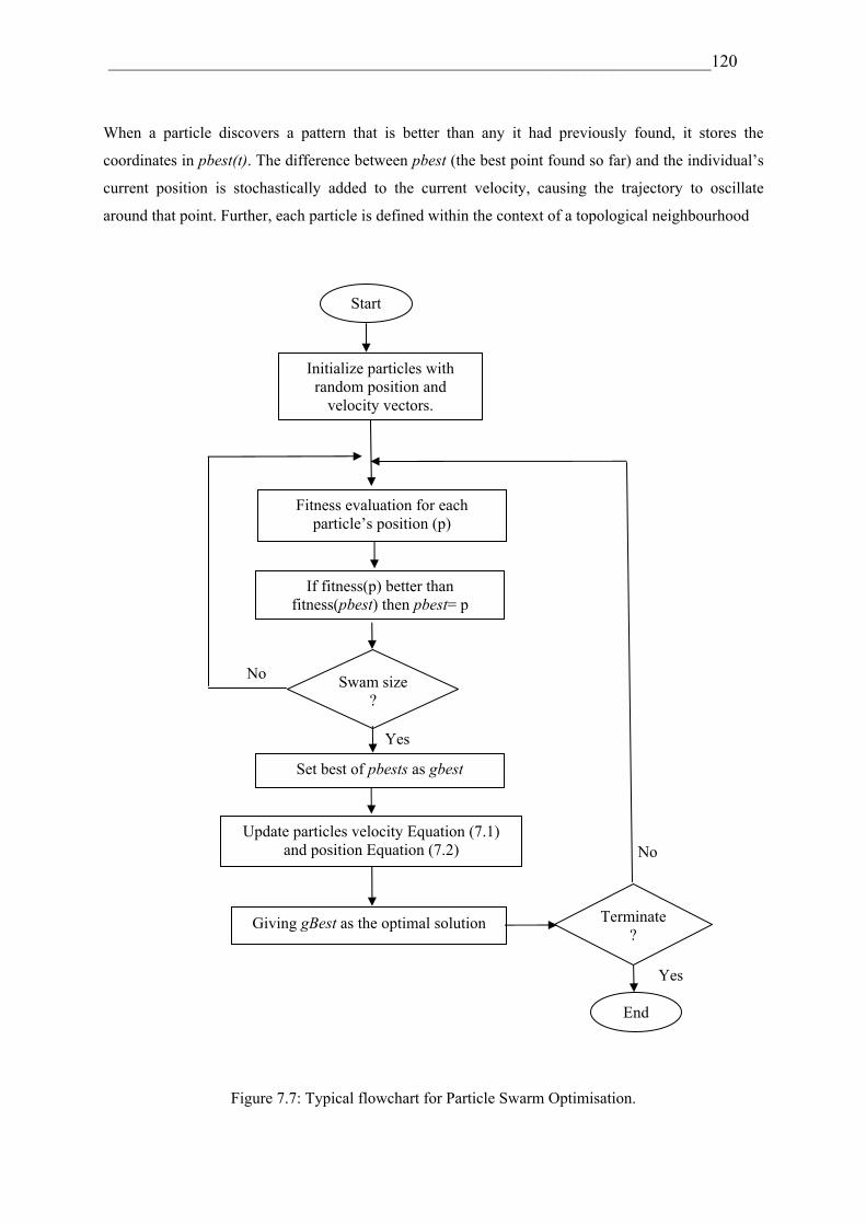
_____________________________________________________________________120
When a particle discovers a pattern that is better than any it had previously found, it stores the
coordinates in pbest(t). The difference between pbest (the best point found so far) and the individual’s
current position is stochastically added to the current velocity, causing the trajectory to oscillate
around that point. Further, each particle is defined within the context of a topological neighbourhood
Figure 7.7: Typical flowchart for Particle Swarm Optimisation.
Yes
No
Yes
No
Initialize particles with random position and
velocity vectors.
If fitness(p) better than fitness(pbest) then pbest= p
Terminate ?
Fitness evaluation for each particle’s position (p)
End
Start
Update particles velocity Equation (7.1) and position Equation (7.2)
Set best of pbests as gbest
Giving gBest as the optimal solution
Swam size ?

_____________________________________________________________________121
comprising itself and some other particles in the population. The stochastically weighted difference
between the neighbourhood’s best position gbest(t) and the individual’s current position is also added
to its velocity, adjusting it for the next time step. These adjustments to the particle’s movement
through space cause it to search around the two best positions, as shown in the equation below:
))()(())()(()()1( 2211 txtgbestrtxtpbestrtwvtv (7.1)
where w is the inertia weight that can be either a constant or a value that changes linearly with the
time; φ1 and φ2 are called “cognitive” and “social” parameters, respectively, and are random positive
constants that weight the influence of the two different swarm memories; and r1 and r2 are random
numbers between 0 and 1.
After the velocity vector had been calculated, the positions of the particles were updated according to
the equation below:
)1()()1( tvtxtx (7.2)
PSO was utilised in the Ad hoc network to satisfy some network requirements and develop routing
protocol, as exemplified by papers [21] and [22]. Also, the PSO algorithm was involved in sensor
networks to create energy-efficient networks, as in papers [23] and [24].
7.5 Comparison between GA and PSO
In this section, the main differences between the two investigated algorithms, GA and PSO, will be
presented. While both algorithms use the fitness concept, they differ in other concepts that are listed in
the table below.
Table 7.2: GA and PSO comparison.
GA PSO
1. Implements the survival of the
fittest
All its particles kept as members of the population through
the course of the run
2. Has selection operation Has no selection operation
3. Has crossover algorithm The adjustment toward the best p(t) and g(t)
4. Has mutation algorithm Balance is achieved through the inertial weight factor (w)

_____________________________________________________________________122
7.6 Intelligent MANET Optimisation
In contrast to the traditional problem solving techniques [6], the metaheurstic algorithms are often
much faster and more adaptable to changes in the environment because the knowledge regarding how
to solve a problem is contained in the collection of individual solutions that has survived up to that
point. This important characteristic has led to the utilisation of the evolutionary algorithms in MANET
routing protocol optimisation.
In this thesis, the GA and PSO metaheurstic optimisation techniques are employed to search for the
best fitted parameters for the proposed intelligent system; the Optimiser compares and evaluates the
performance of the routing protocol in operation with the performance of other protocols in the same
network context.
7.6.1 Determined the Network Context Cases
Before examining the two algorithms as Optimisers, a validation case (Table 7.3) was constructed to
contain all the possible cases for the two input contexts, network size and average mobility. For
example, Case 1 has a large and fast network, whereas Case 9 has a small and slow network.
Table 7.3: Validation cases.
Case no. Network size Average mobility (m/s)
Case 1 Large Fast
Case 2 Large Medium speed
Case 3 Large Slow
Case 4 Medium Fast
Case 5 Medium Medium speed
Case 6 Medium Slow
Case 7 Small Fast
Case 8 Small Medium speed
Case 9 Small Slow
To convert the label of the network sizes (large, medium, and small) and average mobility (fast,
medium, and slow speed) into quantitative values, each context parameter was classified into three

_____________________________________________________________________123
fields, as shown in Table 7.4 for the network size and Table 7.5 for the average mobility. The data
collected for the network size started from a lower limit of 4 nodes and ended up with an upper limit
of 64 nodes, whereas the data collected for the average mobility started from 0 (m/s) and ended up
with 20 (m/s).
The row (From - to) in Table 7.4 classified MANET by the following size criteria:
A small network: 4 nodes ≤ small network ≤ 17 nodes
A medium-sized network: 18 nodes ≤ medium network ≤ 36 nodes
A large network: 37 nodes ≤ large network ≤ 64 nodes.
Table 7.4: Network size classifications.
Network size Small Medium Large
From - to 4 - 17 18 - 36 37 - 64
The cases studied 8 20 62
The row (From - to) in Table 7.5 classified MANET by the following mobility criteria:
A slow network: 0 (m/s) ≤ slow network ≤ 6 (m/s)
A network with medium speed: 6 (m/s) ≤ medium speed network ≤ 13 (m/s).
A fast network: 20 (m/s) ≤ fast network ≤ 13 (m/s).
Table 7.5: Average mobility classifications.
Mobility (m/s) Slow Medium Fast
From - to 0 - 6 6.1 - 13 13.1 - 20
The cases studied 3 11 18
Then, for each classification field (column), one value is randomly selected to represent the field, as
shown by the last rows in Tables 7.4 and 7.5. For example, number 8 selected randomly from the
range (4 nodes ≤ small network ≤ 17 nodes) to present a small network. Therefore, the numbers in the
second rows of Tables 7.4 and 7.5 will replace the labels in Table 7.3 to represent the network context
that will be considered by the GA and PSO Optimisers. The final values are presented in the second
and third columns of the validation table for each Optimiser in Tables 7.6 and 7.7.

_____________________________________________________________________124
7.6.2 The Optimisers Configurations
The two algorithms GA and PSO were employed as MANET Optimisers to find and select the
optimum routing protocol based on the output performance. Both GA and PSO Optimisers were
programmed in MATLABTM.
The NF models were supplied to both Optimisers; where each output parameter was modelled
separately against the input parameters, each Optimiser normalizes the five performance parameters
then merges them into one equation (cost function), and performs calculations for this equation in both
Optimisers. There are many methods [25] to implement a parameter’s normalization; the selected
method depends on the available and known data. Thus, for the normalization in this thesis, the
parameters depend on the equation below, as the maximum and the minimum values are known for
each parameter:
Normalized performance parameterminmax
min
parameterparameter
parameterparameter
(7.3)
The cost function is the Mean Square (MS) of the normalized performance parameter, as shown
below:
Cost function 5
)1()()()( 22222 ThroughputDelayLoadDatadropRA (7.4)
From the Optimiser’s decision it can be concluded that, depending on the cost function, it will select
the routing protocol with the minimum MS to be the optimum routing protocol for that iteration. For
each iteration (or generation) this selection process will be repeated.
The GA and the PSO optimisation process will result in a number of solutions equal to the iteration or
the generation number. The selected solution, that is the optimum routing protocol, will be the one
with the best objective (the minimum MS).
7.6.3 MANET Optimisation
Each Optimiser needs to be supplied with two inputs; the network size and the nodes average mobility
to start its computing. Nine cases were studied based on Table 7.3, as in each case the inputs selected
depended on the second rows of Tables 7.4 and 7.5.
7.6.3.1 GA MANET Optimiser
The GA Optimiser will base its decision on the outputs of the neuro-fuzzy models to find the optimum
protocol that must be adopted. The GA was set with 3 bits of chromosome length for the three

_____________________________________________________________________125
parameters (network size, average mobility, and protocol’s name), with the chromosome value
randomly selected between 0 and 250 and then converted to binary. The population size was 10 with
average ranking, the mutation was 0.06, and the crossover probability was 0.95. Finally, the GA went
through 12 generations to find the optimal solution. Table 7.6 shows the GA’s optimum routing
protocol solution for each case, the solution best objective amplitude, and the generation number for
that solution.
Table 7.6: Genetic Algorithm module results.
GA inputs GA outputs
Case no.
Network
size
Average
mobility (m/s)
Routing
protocol
Best
objective
Generation
no.
case 1 62 18 AODV 0.5288 10
case 2 62 11 OLSR 0.4874 11
case 3 62 3 OLSR 0.9596 10
case 4 20 18 AODV 0.976 1
case 5 20 11 DSR 1.0959 1
case 6 20 3 DSR 1.0035 1
case 7 8 18 AODV 0.9983 8
case 8 8 11 AODV 1.0718 1
case 9 8 3 DSR 0.9981 10
The Pseudo-code for MANET GA is shown in Figure 7.8.
Figure 7.8: MANET GA pseudo-code.
1. Generate initial population of chromosomes of size 10:x1,x2,x3...,x10 2. Repeat 3. Calculate the fitness of each chromosome: f(x1), f(x2),..., f(x10) 4. Evaluate the individual fitnesses of the population. 5. Select pairs of average-ranking individuals to reproduce. 6. Select a pair of chromosomes for the crossover and the mutation. 7. process. 8. Change the genes values to the offspring chromosomes. 9. Place the resulting chromosomes in the new population. 10. If the size of the new generation is not equal to 10 go to 3 11. Replace the current chromosome population with the new population. 12. Until terminating condition

_____________________________________________________________________126
7.6.3.2 PSO MANET Optimiser
The PSO Optimiser was set with three-dimension swarm; the dimensions represent the inputs
(network size, average mobility, and protocol’s name). The size of the swarm was 10, which was
iterated 10 times; the error accepted was set to be less than 1×10⁻¹⁰. The PSO Optimiser used the
practical swarm optimisation for the velocity and the position equations, as in Equations (7.1) and
(7.2). The Pseudo-code for MANET PSO is shown in Figure 7.9.
Figure 7.9: MANET PSO Pseudo-codes.
The optimum routing protocol selected by PSO with its best objective and its iteration number is
shown in Table 7.7.
Table 7.7: Practical Swarm Optimisation module results.
PSO inputs PSO outputs Case
no. Network
size
Average mobility
(m/s)
Routing
protocol
Best
objective
Iteration
no.
case 1 62 18 AODV 0.324004 7
case 2 62 11 OLSR 0.323958 1
case 3 62 3 OLSR 0.323958 5
case 4 20 18 AODV 0.324002 8
case 5 20 11 DSR 0.323958 9
case 6 20 3 DSR 0.323962 1
case 7 8 18 AODV 0.518232 5
case 8 8 11 AODV 0.570085 6
case 9 8 3 DSR 0.323977 7
1. Initialize the three dimensions swarm, 2. Do: 3. For each particle: 4. Calculate fitness value, 5. If the fitness value is better than the best fitness value 6. (pbest) in history, 7. Set current value as the new pbest, 8. End 9. Find in the best pbest 10. Set best pbest as the new gbest, 11. Calculate particle velocity according to the velocity equation 12. Update particle position according to the position equation 13. While maximum iterations not equal to 10 or minimum accepted error 14. is not less than 1×10⁻¹⁰.

_____________________________________________________________________127
7.6.4 Creating the Validation Table
Tables 7.6 and 7.7 show that GA and PSO Optimisers chose the same routing protocols for the same
cases, but most importantly, that the tables’ results confirm that the Optimisers select different routing
protocols through different cases.
To illustrate the point of view that an optimum routing protocol for a MANET context cannot be the
same as for another context, and to demonstrate a possible scenario that could happen in MANET, a
new validation table (Table 7.8) was established which listed all the possible changes to the two
network context parameters for network size and average mobility.
Table 7.8: The validation table: Optimiser selection depending on input context.
First context Optimiser output Second context Optimiser output
Network
size
Average
mobility (m/s) Routing protocol
Network
size
Average
mobility (m/s) Routing protocol
62 18 AODV 62 3 OLSR
62 18 AODV 8 18 AODV
62 18 AODV 8 3 DSR
62 18 AODV 62 11 OLSR
62 18 AODV 20 18 AODV
62 18 AODV 20 11 DSR
8 3 DSR 8 11 AODV
8 3 DSR 20 3 DSR
8 3 DSR 20 11 DSR
8 3 DSR 8 18 AODV
8 3 DSR 62 3 OLSR
8 3 DSR 62 18 AODV
20 11 DSR 20 3 DSR
20 11 DSR 8 11 AODV
20 11 DSR 8 3 DSR
20 11 DSR 20 18 AODV
20 11 DSR 62 11 OLSR
20 11 DSR 62 18 AODV

_____________________________________________________________________128
Table 7.8 includes the solutions for the Optimisers (GA or PSO as they select the same solution). After
supplying the Optimiser with the first context, it will choose a solution that is most of the time
different than its solution for the second context. The table shows the selection of different routing
protocol depending on the input context. Table 7.8 has two main columns: the first main column for
the first input context and the Optimiser selected routing protocol, and the second main column for the
second input context and the Optimiser selected routing protocol. For example, for network with 62
nodes and 18 m/s average mobility the routing protocol selected was AODV, but when the context
changes and the network average mobility is reduced to 3 m/s, OLSR is selected as the optimum
routing protocol.
7.6.5 MANET Optimisers Selection
The GA Optimiser characteristic will be compared with the PSO Optimiser characteristic, based on
Clerc and Kennedy statement about PSO [18] which says, “Particle swarm optimisation comprises a
very simple concept and paradigms; it can be implemented in a few lines of computer code. It requires
only primitive mathematical operators, and is computationally inexpensive in terms of both memory
requirements and speed [19].”
a. GA is more complicated than PSO and includes many algorithms for encoding, ranking, cross
over, and mutation. PSO is much simpler than GA as PSO computation relies on two basic equations.
b. GA requires more time in the computation process because of the number of algorithms to be
processed. As such, few PSO computer codes can make the PSO Optimiser faster than the GA
Optimiser at finding the solutions.
Comparing the efficiency of the two techniques quantitatively, the best objective in each of the fifth
column of Tables 7.6 and 7.7 were studied. After examining the two columns, it shows that, in
general, the GA best objective was always higher in value than the PSO best objective. For example,
in Case 9, when network size was 8 nodes with average mobility 3 m/s, the routing protocol selected
was DSR with GA best objective = 0.9981 and PSO best objective = 0.323977. This clearly shows that
PSO have the minimum MS.
These comparison results evaluate each Optimiser; on this basis, a decision made to implement PSO
techniques as an Optimiser in the I-MAN routing protocols optimisation system.

_____________________________________________________________________129
7.7 Summary
In this chapter, the necessity of utilising the Artificial Intelligence (AI) algorithms for optimizing
MANET has been highlighted because of the AI’s ability to adapt to changes in the environment and
its algorithms’ fast convergence. In this chapter, the sequence operations for each GA and PSO
technique were also explained in detail. Furthermore, two MANET Optimisers were created: one with
GA and the second with PSO. The results show that both Optimisers selected the same routing
protocols for the same specified context.
Subsequently, a validation table was created to include all possible context changes. The results in the
table clearly show that the Optimiser selects a different routing protocol in different cases. Also, the
validation table results confirm that the changes in the network context will affect the network
performance; therefore, for a better network performance, the Optimiser will select a different routing
protocol if the context changes. Having evaluated the two Optimisers in this chapter, it was concluded
that the PSO optimisation technique will be the optimisation technique used in the I-MAN routing
protocols optimisation system.
7.8 References
[1] J. Pearl, “Heuristics: Intelligent search strategies for computer problem solving,” Addison-
Wesley, p. vii, New York, 1984.
[2] M. Dorigo, M. Birattari, and T. Stűtzle, “Ant colony optimisation,” IEEE Computational
Intelligence Magazine, vol. 1, no. 4, pp. 28–39, 2006.
[3] C. Reynolds, “Evolutionary Computation and its application to art and design,” [Online],
available on: http://www.red3d.com/cwr/evolve.html, [accessed on Sep. 17, 2010].
[4] “Particle Swarm Optimisation,” [Online], available on: http://www.swarmintelligence.org/,
[accessed on Oct. 22, 2010].
[5] T. Bäck, “Evolutionary Algorithms in theory and practice,” Oxford, NY, 1996.
[6] “Evolutionary Computation”, Sci-Tech Encyclopedia, McGraw-Hill concise Encyclopedia of
Science and Technology, 5th Edition, McGraw-Hill, 2004.
[7] “Swarm Intelligence,” [Online], available on:
http://www.sce.carleton.ca/netmanage/tony/swarm.html, [accessed on Sep. 17, 2010].
[8] “Swarm Intelligence introductory resources” [Online], available on:
http://staff.washington.edu/paymana/swarm/, [accessed on Oct. 7, 2010].

_____________________________________________________________________130
[9] J. H. Holland, “Adaption in Natural and Artificial Systems”, the University of Michigan Press,
Ann Arbor, 1975.
[10] “Applications of genetic algorithms in Chemistry,” [Online], available on:
http://www.tc.bham.ac.uk/~roy/Research/ga.html, [accessed on Oct. 12, 2010].
[11] J. S. Smith, “Evolving a Better Solution,” Developers Network Journal, March issue, 2002,
[Online], available on: http://www.dnjonline.com/, [accessed on Sep. 19, 2010].
[12] Genetic algorithm - Operation of a GA, “Genetic algorithm - Operation of a GA: Encyclopaedia
II - Genetic algorithm - Operation of a GA,” [Online], available on:
http://www.experiencefestival.com/a/Genetic_algorithm_-_Operation_of_a_GA/id/5078282,
[accessed on Sep. 19, 2010].
[13] C. W. Ahn and R. S. Ramakrishna, “A genetic algorithm for shortest path routing problem and
the sizing of populations,” IEEE Transactions on Evolutionary Computation, vol. 6, no. 6, pp. 566–
579, 2002.
[14] B. Sun, S. Pi, C. Gui, Y. Pi, C. Gui, Y. Zeng, B. Yan, W. Wang, and Q. Qin, “Multiple
constraints QoS multicast routing optimisation algorithm in MANET based on GA,” Progress in
Natural Science, vol. 18, issue 3, pp. 331–336, 2008.
[15] H. Liu, J. Li, Y. Zhang, and Y. Pan, “An adaptive Genetic fuzzy multi-path routing protocol for
wireless Ad hoc networks”, Proceedings of the sixth International Conference on Software
Engineering, Artificial Intelligence, Network and Parallel Distributed Computing (SNPD/SAWN’05),
pp. 468–475,Towson University, Towson, Maryland, USA, 2005.
[16] M. R. Masillamani, A. Jamalipour and G. Uma, “Intelligent MANET,” IEEE International
Conference on Intelligent and Advanced Systems, 2007.
[17] J. Kennedy and R. Eberhart, “Particle Swarm Optimisation,” Proceedings of the first IEEE
International on Neural Networks, Perth, Australia, pp. 1942–1948, 1995.
[18] J. Kennedy, “Swarm Intelligence,” Handbook of Nature-Inspired and Innovative Computing
Integrating Classical Models with Emerging Technologies, editor A. Yomaya, Springer, 2006.
[19] M. Clerc and J. Kennedy, “The particle swarm-explosion, stability, and convergence in a
multidimensional complex space,” IEEE Transactions on Evolutionary Computation, vol. 6, no. 1, pp.
58–73, 2002.
[20] M. Meissner, M. Schmuker and G. Schneider, “Optimised Particle Swarm Optimisation
(OPSO) and its application to artificial neural network training,” BMC Bioinformatics 2006, 7:125,
[Online], available on: http://www.biomedcentral.com/1471-2105/7/125, [accessed on Sep. 19, 2010].

_____________________________________________________________________131
[21] C. Huang, Y. Chuang, and K. Hu, “Using particle swam optimisation for QoS in Ad hoc
multicast,” Engineering Applications of Artificial Intelligence, vol. 22, issue 8, pp. 1188–1193, 2009.
[22] S. Rajagopalan and C. Shen, “ANSI: A Swarm Intelligence-based unicast routing protocol for
hybrid Ad hoc networks,” Journal of Systems Architecture, vol. 52, issue 8, pp. 485–504, 2006.
[23] T. Shih, “Particle Swarm Optimisation algorithm for energy-efficient cluster-based sensor
networks,” IEICE Transactions on Fundamentals of Electronics, Communications and Computer
Sciences, vol. E89–A, no. 7, pp. 1950–1958, 2006.
[24] H. Yang, F. Ye, and B. Sikdar, “A Swarm Intelligence based protocol for data acquisition in
networks with mobile sinks,” IEEE Transactions on Mobile Computing, vol. 7, issue 8, pp. 931–945,
2008.
[25] K. Teknomo, “Normalization,” [Online], available on:
http://people.revoledu.com/kardi/tutorial/Similarity/Normalization.html, [accessed on Jan. 10, 2011].

_____________________________________________________________________132
Chapter 8
System Implementation
8.1 Introduction
The focus in this chapter will be on implementing the intelligent system design outlined in Chapter 4.
To create a MANET network with an embedded system, many modifications to the original nodes
should be made. Therefore, the main contributions in this chapter are as follows:
1. Embedding the intelligent system in the OpnetTM14 modeller.
2. Implementing the I-MAN routing protocols optimisation system in a case study. The case study
scenario includes important changes in the network context; the use of complicated scenario such as
this is of itself novel to this work, since to our knowledge there has been no simulation scenario which
presents various context changes through one scenario.
3. Evaluating the proposed system by comparing networks operating with and without the intelligent
system, as the performance results are the factors used to evaluate the networks.
The rest of the chapter is organised in the following manner: in Section 8.2, the structure for the
network that utilises the intelligent system is determined; in Section 8.3, the implementation process
for the I-MAN optimisation system in MANET is described in detail, which includes determining the
role for each I-MAN system’s component and the sequence for their operation; in Section 8.4, the
modification to MANET's nodes that enables the intelligent system to function will be explained; and
in Section 8.5, the I-MAN routing protocols optimisation system is tested by the simulation through a
case study that includes different changes in the simulation environment, with the simulation results of
the case study reviewed in this section as well. In Section 8.6, the results are compared and analysed
whereas in Section 8.7 the network cost minimisation function is discussed. In Section 8.8, the
network’s performance is evaluated quantitatively. In Section 8.9, the effect of the Inter-Arrival Time
(TIA) on the performance is investigated. Section 8.10 presents the system limitations and finally,
Section 8.11 illustrates the chapter findings.

_____________________________________________________________________133
8.2 I-MAN Optimisation System with MANET
A decision should be made about two important queries before implementing the intelligent system in
a wireless MANET environment; these queries are twofold:
1. The need for the intelligent unit to be in decision node, and
2. The need for embedding the intelligent unit in all MANET nodes.
The forthcoming sections will discuss and clarify these two issues and then come to a decision as to
what the network will be based on in the implementation stage.
8.2.1 Optimisation Unit in Intelligent Node Obviously, the Ad hoc network depends on one routing protocol to route the packets from source to
destination; this means that all Ad hoc nodes should share the same routing protocol at once (except
the zone protocols). Therefore, deciding the optimum routing protocol is not an individual node’s task
that could be concluded independently from other nodes, as each node cannot decide its operating
routing protocol without considering and referring to the other network nodes.
Therefore, referring the routing protocol decision to one intelligent node is crucial, as it should have a
good knowledge about the network. Thus, in this research, the responsibility of deciding on the one
suggested routing protocol is to be undertaken by a single node. After consulting all other network
nodes, the node will then command the network to operate on a specific protocol. An intelligent
module would be embedded in the decision node (optimisation unit), to support the node’s decision
regarding the optimised routing protocol selection. This node will be called the “Intelligent node,” and
should have the computation capability to process the selected optimisation technique.
In this research, the optimisation of the Ad hoc routing protocol has been designed to accommodate an
intelligent unit for the whole network. If another factor is to be considered, such as the data rate, the
decision issue will not be important as each individual network node can send its packets at a rate that
the node is comfortable with. In this case, the intelligent unit could be embedded in each network node
for an individual decision and each node could decide its optimum data rate.
To imagine this decision assumption in an Ad hoc realistic situation or any emergency situation, the
Intelligent node represents the intelligent device in the control panel which advises a group of people
via their devices, as shown in Figure 8.1. For example, a battle field (as in Figure 2.3) where the group
leader’s laptop represents the Intelligent node.
As known MANET devices have a limited battery life [1], by centralizing the optimisation process in
one Intelligent node, other network nodes will be relieved from the data processing. This will also save

_____________________________________________________________________134
the MANET nodes’ power and time, as the other network nodes duty will be supporting the decision
process by forwarding periodic Topology packets to the Intelligent node.
Figure 8.1: Intelligent node with other MANET nodes.
To develop the intelligent system so that the system can overcome the MANET power consumption
problem [1], and to give the intelligent system a better chance of practical implementation in reality,
MANET could be part of the Wireless Mesh Network (WMN) [2]-[3]; MANET could be one of the
end-connected components of WMN wherein the intelligent system is centralized in the mesh router.
MANET nodes could be the MWN client, as shown in Figure 8.2, in which MANET network is
connected to the backbone of the WMN through a mesh router. In this case, one of the WMN routers
(the red arrows) will have the responsibility of optimising the routing protocol for the whole MANET.
In this case, more power and time will be saved for MANET as the MWN router will receive
information and forward its decision from/to the MANET nodes. Figure 2.1 in Chapter 2 can also help
to adapt this idea by embedding the intelligent unit in the fixed network router that will receive
information and forwarding the decision from/to the mobile network.
MANET
Topology and Decision packets traffic
Intelligent node
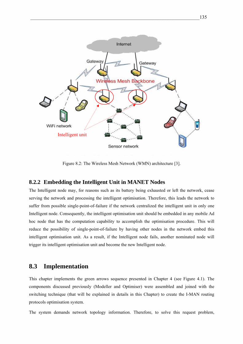
_____________________________________________________________________135
Figure 8.2: The Wireless Mesh Network (WMN) architecture [3].
8.2.2 Embedding the Intelligent Unit in MANET Nodes The Intelligent node may, for reasons such as its battery being exhausted or left the network, cease
serving the network and processing the intelligent optimisation. Therefore, this leads the network to
suffer from possible single-point-of-failure if the network centralized the intelligent unit in only one
Intelligent node. Consequently, the intelligent optimisation unit should be embedded in any mobile Ad
hoc node that has the computation capability to accomplish the optimisation procedure. This will
reduce the possibility of single-point-of-failure by having other nodes in the network embed this
intelligent optimisation unit. As a result, if the Intelligent node fails, another nominated node will
trigger its intelligent optimisation unit and become the new Intelligent node.
8.3 Implementation
This chapter implements the green arrows sequence presented in Chapter 4 (see Figure 4.1). The
components discussed previously (Modeller and Optimiser) were assembled and joined with the
switching technique (that will be explained in details in this Chapter) to create the I-MAN routing
protocols optimisation system.
The system demands network topology information. Therefore, to solve this request problem,
Intelligent unit

_____________________________________________________________________136
Topology packets are sent to the I-MAN routing protocols optimisation unit, as shown in Figure 8.1.
Each Topology packet contains the node’s mobility and the routing protocol in use.
The optimisation block diagram shown in Figure 8.3 illustrates the optimisation unit embedded in the
Intelligent node, and represents the operations of the I-MAN optimisation unit in sequence. The unit
consists of the Communication Gate, Information Stack, Optimiser, Modeller, and Decision Maker. As
given below.
Figure 8.3: I-MAN optimisation unit blocks diagram.
First, the Intelligent node’s Communication Gate will forward the Topology packets received from the
network nodes to the Information Stack. Next, the Information Stack will deduce the current network
context (the requested information parameters are: network size and average mobility). Afterward, the
Information Stack will update the Optimiser with the new context (the roles of the Information Stack
are explained in more detail further on; see the flowchart shown in Figure 8.4). The Optimiser then
generates its solution for the current context with the support of the Modeller to predict the network
performance metrics for each solution. The protocol’s performance metrics help the Optimiser to not
only evaluate the routing protocol in operation, but also determine the optimum routing protocol, as
the optimum protocol for the network will be selected based on its performance. The selected routing
protocol should have the best cost, which results from a combination of the desired parameters for less
data drop, less delay, lower loads, less RA, and higher throughput. The decision will then be fed to the
Decision Maker. The latter will conclude the switch time and reference it with the new optimum
Intelligent node
Optimisation unit
Information Stack Optimiser Decision Maker
Modeller
Communication Gate
MANET nodes

_____________________________________________________________________137
routing protocol in the Decision packet. Next, the Decision Maker will send the Decision packet to the
Communication Gate. Finally, the Communication Gate will start feedback of the Decision packets to
the network nodes.
Figure 8.4 shows a flowchart of the I-MAN routing protocols optimisation system which focuses on
the system implementation through the time scale. First, the system parameter should be initialised;
here, OPT is the parameter that represents the optimisation unit condition. If OPT = 0 that means this
is the first run for the unit, and also means that the unit did not receive Topology packets before (the
current context information) from the network. Whereas if OPT > 0, this means that the Optimiser was
previously activated and chose the optimum routing protocol after receiving previous Topology
packets.
After the network nodes send the Topology packets to the Intelligent node, the Information Stack will
start its procedure, as shown by the flowchart sequence in Figure 8.4 and outlined below:
The first role is to count and gather each packet received from the Communication Gate to conclude
the total network size, utilising the nodes counter.
The second role is to extract the node’s mobility and the protocol name in operation from the node’s
Topology packet; then the node’s mobility will be added with the others nodes mobility.
The third role is to buffer all the network topology information until time T1,
as T1 = current simulation time + Threshold_1, (8.1)
where Threshold_1 is the sent delay allowances, or the estimated time for all the network nodes’
Topology packets to be received by the Intelligent node.
The fourth role is to calculate, at time T1, the Optimiser requested parameters; network size (nodes
counter); and Average Mobility. The total of nodes counted will be the network size, whereas the
average nodes mobility will be calculated by adding up all the nodes’ mobility and then dividing the
result by the network size previously calculated.
The fifth role is to compare the Information Stack context results: the network size and the average
mobility. If OPT = 0, then these results will be forwarded to the Optimiser directly but if OPT > 0,
then the results should be compared to or matched with the network context from the previous period
(that should be stored in the Information Stack). If the matching procedure result is negative, this
means that the contexts are different and there will be new inputs to the PSO Optimiser. However, if
the matching procedure result is positive and the context values are the same, then that means the
network context did not change. In such case there is no need to activate the Optimiser as the same
previous decision will be reached. Also, there will be no need to send Decision packets from the
Intelligent node to the network nodes.

_____________________________________________________________________138
Figure 8.4: I-MAN routing protocols optimisation system implementation flowchart.
Send current node context packet (Node mobility and protocol name)
No
Yes
Simulation time = T2
Forward Nodes counter and average Mobility to Optimiser
Yes
Yes
Simulation time = = T1
OPT > 0
No
Average mobility = Pervious Average mobility Nodes counter = Pervious Nodes counter
No
Yes
No
Yes
The Optimiser generates solutions and tests them with the support of the Modeller prediction
Switch to the optimum routing protocol
?
Nodes counter = Nodes counter +1 Mobility = Mobility + Node mobility
Nodes counter = 0 Mobility = 0 T1= Simulation time + Threshold_1 T2 = Simulation time + Threshold_2
Start
Average mobility = Mobility/ Nodes counter Protocol name = Current Protocol
More Packets No ?
Yes
No ?
Ending Time > = Simulation time
Yes ?
Determined the optimum routing protocol OPT= OPT+1
No
?
?
Optimum protocol = Current protocol?
End
Intelligent node
Network nodes OPT = 0

_____________________________________________________________________139
Figure 8.4 presents the Modeller role in predicting the network performance for each protocol and then
sending it to the Optimiser to determine the optimum protocol. The flowchart also illustrates the
Decision Maker’s role after the Optimiser concludes its decision (that is, sends the Decision packets).
The packets contain the new optimum routing protocol name plus switching simulation time (T2) to
the Communication Gate,
as T2 = current simulation time + Threshold_2, (8.2)
where Threshold_2 is the delivery delay allowances or the estimated time for the Decision packets
sent from the Intelligent node to reach all the network nodes.
The Decision Maker will decide the exact simulation time T2; as in, the time that the network nodes
should adopted the new optimum protocol mechanism. The Communication Gate will then broadcast
the packets to all the network nodes. If the optimum routing protocol is similar to the current routing
protocol in operation, then the Decision Maker will not send Decision packets to the Communication
Gate.
8.4 MANET Nodes Modification
To evaluate the intelligent system, the I-MAN routing protocols optimisation system was implemented
with the support of the OpnetTM14 modeller that uses C++ programming language.
Two major modifications should be implemented to the wireless network nodes models in the
OpnetTM14 modeller: the first is for the node that will embed the intelligent unit (that is, Intelligent
node); the second is for the other network nodes that will embed the switching technique. The
following sections will illustrate the modification. Mainly, the modification (the optimisation unit or
the switching technique) was in the MANET node's IP process model. Figure 8.5 shows the original
IP process model for MANET nodes in the OpnetTM14 modeller.

_____________________________________________________________________140
Figure 8.5: The original IP process model for MANET node in OpnetTM14 modeller.
8.4.1 Creating the Intelligent Node In Section 8.2 a conclusion was drawn that, in order to create the intelligent optimisation system, at
least one of the OpnetTM14 modeller MANET nodes should embed the intelligent optimisation unit in
their process model. Therefore, the entire intelligent optimisation block diagram in Figure 8.3 should
be included and embedded in the Intelligent node. As illustrated in Figure 8.6, the Information Stack
component is divided between the init and idle processors (the thin black arrows). Therein, the green
process model with the title NF-PSO contains two major components: the Optimiser and the Modeller
(the double black arrow). Finally, the Decision Maker component is based in the idle processor (the
thicker black arrow).

_____________________________________________________________________141
Figure 8.6: The IP process model for Intelligent MANET node in OpnetTM14 modeller.
8.4.1.1 Embedding the Information Stack The init process creates and initializes two counters: the Nodes and the Mobility counters. When a
Topology packet is received from the MANET nodes, the init process will send an interruption
command to the idle process. The Nodes counter will increase by one with every received packet. The
packets collection process will continue until T1. At time T1, the value of the Nodes counter represents
the total number of the network nodes in the MANET.
The Topology packet also contains the node’s mobility. For every Topology packet that arrives, the
node’s mobility will be extracted and added to the Mobility counter; then the packet will be destroyed.
The Mobility counter will keep summing the nodes’ mobility until time T1, when the average mobility
is calculated by dividing the Mobility counter value by the Node counter.
8.4.1.2 Embedding the NF Modeller After time T1, and after calculating the MANET context parameters, the idle process will send an
interruption command to operate NF-PSO process. Then the network performance will be predicted
using the network performance models.
Information Stack
Decision Maker Optimiser and Modeller

_____________________________________________________________________142
In the NF-PSO process model, the neuro-fuzzy (NF) Modeller created is based on the Sugeno
modelling approach. Some of the details that are needed to program the Modeller, such as the type of
the input membership functions, the number of rules for each performance model, and the constant
parameters, are borrowed from the NF MANET performance models created in Chapter 6, wherein 15
models were developed.
Support from the Modeller ensures adoption of the optimum protocol by the Optimiser. Thus, to select
the best protocol, the I-MAN Modeller generated the performance models (data drop, delay, load,
retransmission attempt, and throughput) for MANET routing protocols depending on the network
context
8.4.1.3 Embedding the PSO Optimiser For each iteration loop, the Modeller will send the performance parameters values to the Optimiser
that will start the optimisation process. To create the PSO Optimiser, the optimisation technique is
embedded in an NF-PSO process model based on the practical swarm optimisation velocity Equation
(7.1) and position Equation (7.2) [4].
PSO, the process that inspired from nature, was set with three dimensions swarm to represent the two
inputs: network size and average mobility, and the one output the routing protocol. The size for the
swarm was 10, iterated ten times, with an accepted error of less than 1×10⁻¹⁰. The PSO Optimiser
objective function is based on the cost function in Equation (7.4). In this case study, the value for w
was 0.7298; the values for φ1 and φ2 were 1.49618, whereas r1 and r2 were calculated randomly. The
best objective, the performance parameters least Mean Square (MS), will determine the optimum
protocol, where the selected protocol has a combination of the parameters for the least normalized data
drop, the least normalized load, the least normalized delay, the least normalized RA, and the highest
normalized throughput. The Optimiser results will then be forwarded to the Decision Maker.
8.4.1.4 Embedding the Decision Maker First, the Decision Maker compares the Optimiser results with the current routing protocol in
operation. If the comparison results are the same, then there will be no action from the Decision
Maker. However, if the comparison results are different, the Decision Maker will start to calculate T2
and then create the Decision packet. The Decision Maker broadcasts these packets to all MANET
nodes. The packet contains the routing protocol’s name and switching time (T2), or time at which all
nodes should trigger the switching technique and adopt the suggested new protocol.
8.4.2 Creating the MANET Nodes The original MANET node model should be modified to be able to perform the extra roles, as listed
below:

_____________________________________________________________________143
a. Send periodic Topology packet: each node in MANET creates a Topology packet containing its
nodes’ mobility and the protocol in use; the node then sends this packet to the Intelligent node at a
predefined time.
b. Receive the Decision packet: when a MANET node receives the Decision packet, it will extract
the new routing protocol and the switching time from the packet (then the packet will be destroyed).
c. Adapt the switching protocol technique: the node will compare the switching time with the
current simulation time. When the switching time is equivalent to the current simulation time, the node
will use its switching technique to switch to the new routing protocol. As shown by the blue arrow in
Figure 8.7, the (SW_Protocol) arrow leads the node to initialise the process of adapting the new
routing protocol.
d. Buffering the data packets: packets are buffered until the new routing protocol is established.
Figure 8.7: The IP process model for MANET node that adopts the switching technique in OpnetTM14
modeller.
Switching technique

_____________________________________________________________________144
8.5 Case Study
To evaluate the proposed I-MAN routing protocols optimisation system, it should be implemented in a
realistic scenario where the network context is changing. Also, the network operating the system
should be compared to other networks’ operating routing protocols in the same scenario conditions,
without the system. Therefore, this case study presents one scenario example that addresses different
contexts.
8.5.1 Simulation Environment Four identical MANET simulation scenarios were executed. The same network scenario was
implemented four times: first with the OLSR routing protocol, second with the DSR routing protocol,
third with the AODV routing protocol and fourth with I-MAN. Each scenario ran for 4800 s. Nodes
moving randomly distributed raw packets at 1 Mbps data rate to random destinations. Packets were
generated with Poisson Inter-Arrival time. All scenarios were implemented with five context cases
which lasted for nearly 16 minutes. Table 8.1 explains the context’s duration, network size, and
average mobility.
Table 8.1: The scenario’s list of context.
Context Case Time (minute) Network size Average mobility (m/s)
First 0 ~ 16 16 4 Second 16 ~ 32 55 4 Third 32 ~ 48 55 9 Fourth 48 ~ 64 21 9 Fifth 64 ~ 80 21 17
An image shown in Figure 8.8 for MANET ran context 1 for the fourth simulation, the I-MAN
protocol scenario. The image illustrates the both working and the failed nodes, and also presents the
position of each node at time 0.

_____________________________________________________________________145
Figure 8.8: MANET image representing part of I-MAN scenarios: context 1.
Also, another image in Figure 8.9 for MANET ran Context 2 and Context 3 for the same scenario to
represent the working and the failed nodes. As mentioned before, the nodes are moving arbitrarily so
their position is always changing; therefore, this image does not present the nodes’ positions in
Context 2 and Context 3.

_____________________________________________________________________146
Figure 8.9: MANET image representing part of I-MAN scenario: Context 2 and Context 3.
The last MANET image in Figure 8.10 represents part of the I-MAN scenario with Context 4 and
Context 5. This image presents the working nodes (network size) in this scenario, but not their
positions in Context 4 and Context 5 (network mobility).
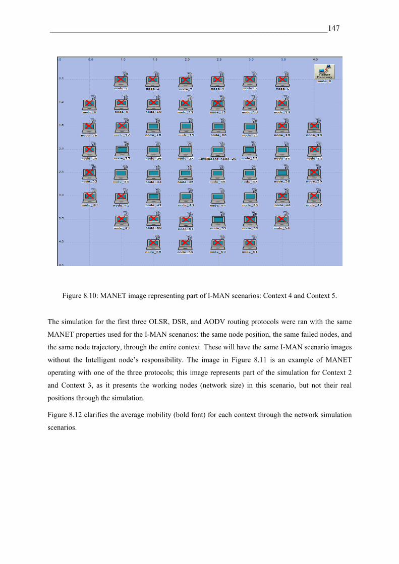
_____________________________________________________________________147
Figure 8.10: MANET image representing part of I-MAN scenarios: Context 4 and Context 5.
The simulation for the first three OLSR, DSR, and AODV routing protocols were ran with the same
MANET properties used for the I-MAN scenarios: the same node position, the same failed nodes, and
the same node trajectory, through the entire context. These will have the same I-MAN scenario images
without the Intelligent node’s responsibility. The image in Figure 8.11 is an example of MANET
operating with one of the three protocols; this image represents part of the simulation for Context 2
and Context 3, as it presents the working nodes (network size) in this scenario, but not their real
positions through the simulation.
Figure 8.12 clarifies the average mobility (bold font) for each context through the network simulation
scenarios.
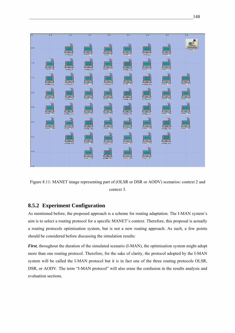
_____________________________________________________________________148
Figure 8.11: MANET image representing part of (OLSR or DSR or AODV) scenarios: context 2 and
context 3.
8.5.2 Experiment Configuration As mentioned before, the proposed approach is a scheme for routing adaptation. The I-MAN system’s
aim is to select a routing protocol for a specific MANET’s context. Therefore, this proposal is actually
a routing protocols optimisation system, but is not a new routing approach. As such, a few points
should be considered before discussing the simulation results:
First, throughout the duration of the simulated scenario (I-MAN), the optimisation system might adopt
more than one routing protocol. Therefore, for the sake of clarity, the protocol adopted by the I-MAN
system will be called the I-MAN protocol but it is in fact one of the three routing protocols OLSR,
DSR, or AODV. The term “I-MAN protocol” will also erase the confusion in the results analysis and
evaluation sections.

_____________________________________________________________________149
Figure 8.12: I-MAN routing protocol adaptations through the simulation period.
Second, in scenario four (I-MAN), the I-MAN protocol could be a combination of the protocols
OLSR, DSR and/or AODV. Therefore, the I-MAN protocol will have the same characteristics of the
adopted protocol. For example, if the I-MAN protocol adopts AODV routing protocol, it will have the
same strengths and weaknesses of the AODV routing protocol mentioned previously in Chapter 4.
Third, in this case study, the first three MANET scenarios (OLSR, DSR, and AODV) were presented
as a flat network, whereas in the fourth scenario for I-MAN, the MANET network was presented as a
cluster network led by the Intelligent node.
Fourth, in the first three scenarios (OLSR, DSR, and AODV), MANET nodes have to send one type
of packet: data packets; whereas in the I-MAN simulation scenario, the network nodes send two types
of packets: data packets and Topology packets.
The types of packets needed for the simulations were defined as follows:
1. Data packets: These packets represent the data sent between the users. The packets’ Inter-Arrival
Time (TIA) was 100 s, which means the data packets will be sent to random destination addresses
every 100 s.
2. Topology packets: employed solely in the I-MAN scenario, each node had to send five Topology
packets through the simulation time to the Intelligent node. The first Topology packet was sent at time
320 s, whereas the other four Topology packets will be sent from time 960 s until the end of the
simulation, with 960 s Inter-Arrival Time.
Fifth, in the I-MAN scenario, there should be a sufficient time (Threshold_1) for the Topology
packets to reach the Intelligent node and a sufficient time (Threshold_2) for the Decision packets to
reach the MANET nodes. Therefore, deciding the amplitude for Threshold_1 and Threshold_2 effects
the simulation dramatically. Thus, the value of Threshold_1 was chosen to be 0.5 s and the value for
Threshold_2 was chosen to be 0.5 s.
Simulation Time 0 min. 16 min. 32 min. 48 min. 1hr 4min 1hr 20min Network size 16 nodes 55 nodes 55 nodes 21 nodes 21 nodes Time Period 16 min. 16 min. 16 min. 16 min. 16 min. Average Mobility 4 m/s 9 m/s 17 m/s I-MAN adaptations AODV DSR OLSR OLSR DSR AODV (Default)

_____________________________________________________________________150
Six, in the I-MAN scenario, the optimiser unit processes the normalization Equation (7.3) and the cost
function in Equation (7.4) to determine the best protocol.
8.5.3 Simulation Results Figure 8.12 illustrates the I-MAN system protocol adaptation through the simulation period against the
network size and the average mobility. The figure shows the I-MAN system’s reaction to each context
change by adopting the ideal routing protocol (choosing the optimum routing mechanism) for that
situation. The I-MAN protocol implements the switching procedure at T2 to switch to different routing
protocol from one period of time to another. The I-MAN scenario started with the default routing
protocol AODV, then implemented the I-MAN system and adapting sequence of the protocols shown
in the figure; the network first switched to the DSR routing protocol, followed by another switch to
OLSR, then a switch back to DSR, and finally, a switch to AODV.
Through the I-MAN simulation scenario, The Optimiser has selected more than one routing protocol.
Table 8.2 shows more details about the I-MAN protocol switching process during the scenario. The
table includes the context case no., the previous routing protocol activated by the network nodes, the
period for each context, the current setting, and the suggested optimum routing protocol (that is, the I-
MAN protocol that should be in operation during the time period mentioned in the table). At the
beginning of the simulation, the I-MAN protocol starts with the default routing protocol AODV
(before triggering the optimisation unit) up to time 320 s. At that time, the nodes will start to send their
current context Topology packets, represented by Context 1 (shown also in Figure 8.8). The I-MAN
Optimiser will select the DSR routing protocol to be the I-MAN protocol for the period (320 s - 960 s).
Therefore, all network nodes after time 320 s (320 + T2) up to 960 s should adopt DSR routing
protocol.
Table 8.2: I-MAN Optimal Selection for the Case Study Scenario.
Current settings Optimal settings
Context Cases
Previous routing protocol
Time (sec) No. of
nodes Mobility
(m/s)
I-MAN protocol acts as
default ---- 0-320 16 4 AODV 1 AODV 320-960 16 4 DSR 2 DSR 960-1920 55 4 OLSR 3 OLSR 1920-2880 55 9 OLSR 4 OLSR 2880-3840 21 9 DSR 5 DSR 3840-4800 21 17 AODV

_____________________________________________________________________151
However, as shown in Figure 8.9, when the network size is increased to 55 nodes as in Context 2,
OLSR is consequently chosen as the I-MAN protocol to route the packets and prevent the network
performance from deterioration. In Context 3, when the nodes’ speeds have increased to 9 m/s, the
Optimiser selects OLSR as well. In this situation, since OLSR matches the previous protocol used
during the previous simulation period, the Intelligent node’s action was not to send Decision packets
to the network nodes.
In Context 4, due to the dynamic nature of MANET, many nodes left the network; the network size
thereby decreased to 21 nodes, as shown in Figure 8.10. As such, the I-MAN Optimiser selects DSR to
operate the network instead of OLSR. However, when the mobility increased to 17 m/s in Context 5,
AODV was the protocol selected to serve the network.
8.6 Comparison and Results Analysis
Visual comparisons between the four routing schemes (AODV, DSR, OLSR, and I-MAN) are
presented in Figures 8.13 through 8.17. The comparisons were presented in terms of data drop, delay,
load, RA, and throughput, respectively.
8.6.1 Data Drop Figure 8.13 shows a comparison of the data drop variation for the four protocols throughout the
simulation time. It can be seen that the I-MAN routing protocol has the lowest data drop followed by
OLSR, then AODV, while the DSR has the largest data drop.
OLSR, a Table-Driven routing protocol that generates routing tables for the entirety of network
destinations, was able to deliver most of the data without dropping it. Therefore, the OLSR data drop
curve was better than the DSR and AODV data drop curves. The simulation data of OLSR (in
Contexts 2 and 3) shows that OLSR was able to handle the scalable network efficiently.
On the other hand, the network scalability causes a noticeable data drop for the On Demand routing
protocols DSR and AODV as a result of establishing routes in a large network.
As compared to the data dropped by DSR and AODV in Context 1, larger amounts of data were
dropped by both in Contexts 2 and 3 (see Figure 8.13). Up to Context 3, DSR and AODV protocols
had approximately the same attitude; in Context 4, however, the AODV routing protocol outperformed
DSR as the AODV data drop was significantly less since the AODV protocol mechanism is adaptable
to highly dynamic networks (see the comparison section in Chapter 4). Finally, in Context 5 the data
drop for the two On Demand protocols was found to be acceptable. In general, AODV performance
was better than DSR as the AODV’s data drop was comparatively less than the DSR’s.

_____________________________________________________________________152
Figure 8.13: OLSR, DSR, AODV, and I-MAN data drop.
As is clearly shown in Figure 8.13, the best data delivery for the entire context is achieved by the I-
MAN protocol, as it has the best data delivery rate. From time (0 ~ 320 s), the I-MAN optimisation
unit was not yet active, therefore resulting in the drop of data. After activating the optimisation unit
(from time 320 s up to the end of the simulation), this data drop was reduced significantly. The I-MAN
system allows each network node a packets buffer to store the packets that could not reach their
destinations. After establishing a new route, the packets will be sent again and, consequently, the data
drop will be notably reduced.
8.6.2 Delay Figure 8.14 shows the delay curves of the four protocols AODV, DSR, OLSR, and I-MAN throughout
the simulation.
Comparing the three protocols’ OLSR, DSR, and AODV delay curves in all the five contexts shows
that the OLSR has the lowest delay curve, followed by AODV, and DSR, which had the highest curve.
The proactive routing protocol OLSR exhibited an excellent delay performance throughout the
simulation’s duration due to the periodic message and MPR mechanism that keeps the nodes’ routing
table updated and helps in delivering the packets without remarkable delay even when the number of
nodes increases.
0
500
1000
1500
2000
2500
3000
3500
4000
0 960 1920 2880 3840 4800
Time(s)
Dat
a D
rop
(bit
s/s)
OLSR
DSR
ADOV
I-MAN
320
Context 1 Context 2 Context 3 Context 4 Context 5 Default

_____________________________________________________________________153
0
0.005
0.01
0.015
0.02
0.025
0.03
0.035
0.04
0.045
0.05
0 960 1920 2880 3840 4800
Time(s)
Del
ay(s
)
OLSR
DSR
AODV
I-MAN
320
Context 1 Context 2 Context 3 Context 4 Context 5 Default
Figure 8.14: OLSR, DSR, AODV, and I-MAN delay.
Higher delay rates were obtained for the On Demand routing protocols AODV and DSR since
whenever a source needs to send packets to a destination, the On Demand routing protocols apply the
Route discovery mechanism if the destination address is not available in the source routing table.
Furthermore, network scalability has an effect on the DSR delay rate, as shown in Figure 8.14,
throughout the simulation time and up to 2880 s. Given the changes in the Contexts 1, 2, and 3, the
DSR delay rate increased as a result of increasing the network size. The delay rate increased because
of the implementation of the DSR's routing cache mechanism (for more detail, refer to the DSR
weaknesses described in the comparisons made by Section 4.4.5.2).
Figure 8.14 also indicates that the I-MAN protocol behaviour varied throughout the simulation time.
From time 0 s up to time 320 s, the delay rate was high because the network was adopting the default
routing protocol (AODV); as such, the intelligent unit was not activated during this period of time.
After time 320 s, the I-MAN optimisation unit became operative and selected the DSR mechanism as
the optimum routing protocol. Consequently, after applying the I-MAN switching mechanism and
adopting the DSR protocol, the network delay rate was clearly reduced. From 960 s up to 2880 s as
represented in Contexts 2 and 3, the I-MAN protocol adopted an OLSR mechanism, yielding an
approximately constant delay rate. In contrast, the I-MAN protocol in Contexts 4 and 5 produced
slightly higher delay rates with acceptable levels.
In Figure 8.14, there was a rapid increment in the delay rate occurring at time 320 s, 960 s, and 3840 s
due to the Decision packets that are sent by the Intelligent node to the network nodes.

_____________________________________________________________________154
8.6.3 Load Figure 8.15 shows the network load graphs operating the four protocols AODV, DSR, OLSR, and I-
MAN through the simulation time.
Figure 8.15: OLSR, DSR, AODV, and I-MAN load.
In comparing the load graphs for the three protocols OLSR, DSR, and AODV throughout all network
context changes, it appears that the DSR routing protocol has the highest load, the AODV the second
highest, whereas the least load was for OLSR routing protocol.
The updating of OLSR routing tables assists the protocol in obtaining the least load, whereas the
AODV sequence number technique aids in the protocol load reduction. On the other hand, DSR load
was the highest through the whole simulation, especially in Contexts 2 and 3, as the network
scalability dramatically affected DSR operation and created load over the entire network. In Contexts
4 and 5, however, the load was reduced drastically as a result of the network size reduction. In these
Contexts (4 and 5), the DSR multi-routing path strategy pays off, so that if the route established earlier
is broken, then the source will search its route cache for another ready-route to that destination. If a
ready-route is found, the source does not have to establish a new Route discovery and will send the
packets through the second backup route. Therefore, the source will save both time and power.
In Figure 8.15, the I-MAN graph shows the changes in the load, as I-MAN load decreases and
increases following the I-MAN adopted protocol. The graph clearly shows the I-MAN mechanism
switching to different protocol at times 320 s, 960 s, 2880 s, and 3840 s. After 320 s, in Context 1 the
load level was acceptable when the I-MAN Optimiser was activated. During the period from 960 s to
0
20000
40000
60000
80000
100000
120000
140000
160000
0 960 1920 2880 3840 4800
Time (s)
Lo
ad(b
its/
s)
OLSR
DSR
AODV
I-MAN
320
Context 1 Context 2 Context 3 Context 4 Context 5 Default
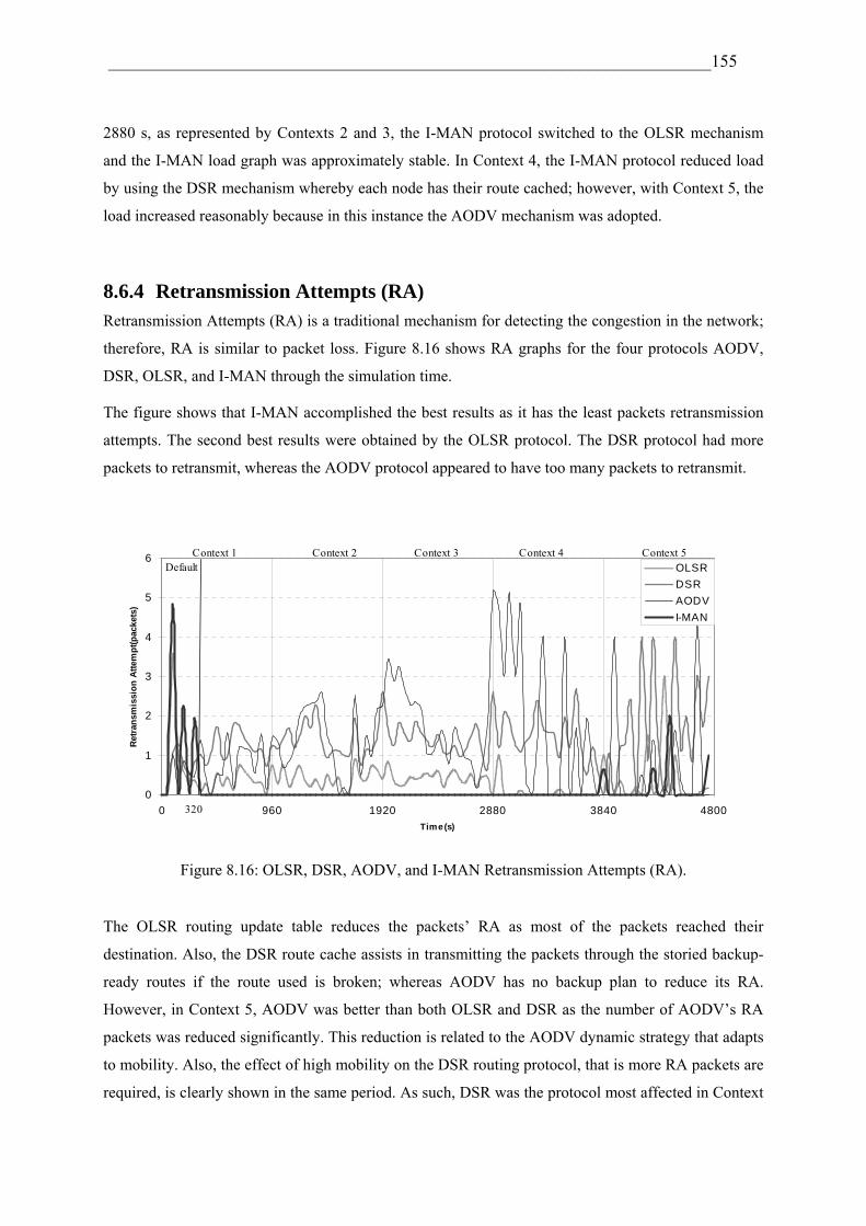
_____________________________________________________________________155
2880 s, as represented by Contexts 2 and 3, the I-MAN protocol switched to the OLSR mechanism
and the I-MAN load graph was approximately stable. In Context 4, the I-MAN protocol reduced load
by using the DSR mechanism whereby each node has their route cached; however, with Context 5, the
load increased reasonably because in this instance the AODV mechanism was adopted.
8.6.4 Retransmission Attempts (RA) Retransmission Attempts (RA) is a traditional mechanism for detecting the congestion in the network;
therefore, RA is similar to packet loss. Figure 8.16 shows RA graphs for the four protocols AODV,
DSR, OLSR, and I-MAN through the simulation time.
The figure shows that I-MAN accomplished the best results as it has the least packets retransmission
attempts. The second best results were obtained by the OLSR protocol. The DSR protocol had more
packets to retransmit, whereas the AODV protocol appeared to have too many packets to retransmit.
Figure 8.16: OLSR, DSR, AODV, and I-MAN Retransmission Attempts (RA).
The OLSR routing update table reduces the packets’ RA as most of the packets reached their
destination. Also, the DSR route cache assists in transmitting the packets through the storied backup-
ready routes if the route used is broken; whereas AODV has no backup plan to reduce its RA.
However, in Context 5, AODV was better than both OLSR and DSR as the number of AODV’s RA
packets was reduced significantly. This reduction is related to the AODV dynamic strategy that adapts
to mobility. Also, the effect of high mobility on the DSR routing protocol, that is more RA packets are
required, is clearly shown in the same period. As such, DSR was the protocol most affected in Context
0
1
2
3
4
5
6
0 960 1920 2880 3840 4800
Time(s)
Ret
ran
smis
sio
n A
ttem
pt(
pac
kets
)
OLSR
DSR
AODV
I-MAN
320
Context 1 Context 2 Context 3 Context 4 Context 5 Default

_____________________________________________________________________156
5.
As shown in Figure 8.16, before operating the I-MAN unit, the default protocol AODV caused many
packets RA up to time 320 s. After time 320 s, when the optimisation unit was activated, the packets
RA was reduced significantly in contexts 1, 2, 3, and 4. This deterioration is related to the packets’
buffer, secured in each node in I-MAN scenario, to hold the un-transmitted packets. However, in
Context 5, the network’s high mobility caused the dropping in data packets that need to re-transmit
again, as shown in Figure 8.16.
8.6.5 Throughput Figure 8.17 shows the throughput graphs for the four protocols AODV, DSR, OLSR, and I-MAN
throughout the simulation time.
Figure 8.17: OLSR, DSR, AODV, and I-MAN throughput.
Comparing the three traditional protocols’ OLSR, DSR, and AODV throughput, it appears that AODV
yielded abundant throughput during the simulation, with OLSR second, and DSR yielding relatively
low throughput.
The AODV protocol was thus able to forward more packets than the other two protocols; this
characteristic confirms the protocol’s adaptability to the network dynamic changes.
Part of the OLSR routing protocol throughput is the OLSR periodic update messages that increase the
OLSR throughput.
0.0E+00
5.0E+05
1.0E+06
1.5E+06
2.0E+06
2.5E+06
3.0E+06
3.5E+06
0 960 1920 2880 3840 4800
Time(s)
Th
rou
gh
pu
t(b
its/
s)
OLSR
DSR
ADOV
I_MAN
320
Context 1 Context 2 Context 3 Context 4 Context 5 Default

_____________________________________________________________________157
Finally, DSR had fewer throughputs since it is not adaptable to the network dynamic changes and it
does not use the periodic message technique.
As shown in the figure, I-MAN throughput results vary depending on the mechanism adopted through
the simulation period.
As shown in Figure 8.17, there is an increase in I-MAN throughput at time 320 s, 960 s, 2880 s, and
3840 s due to the Decision packets forwarded by the network nodes. The reduction in the number of
Decision packets between context 4 and context 5 kept the throughput graph flowing without a
recognizable increase at that time, as the Intelligent nodes have to forward 21 Decision packets.
8.7 The Network Performance Cost Minimisation Function
The previous output performance figures—Figure 8.13 for data drop; Figure 8.14 for delay; Figure
8.15 for load; Figure 8.16 for Retransmission Attempts (RA); and Figure 8.17 for throughput—failed
to clearly show the best routing protocol through the five context changes. For example, OLSR has the
best results in terms of delay and load, whereas AODV has the best throughput. Therefore, a cost
equation, as shown in Equation (8.3), has been suggested to evaluate the performance of the four
protocols for the simulation’s duration.
Cost Minimisation = data drop + delay + load + RA + (1-throughput) (8.3)
To deliver and create the performance cost minimisation graph for each routing protocol, two steps are
needed: first, normalizing the five output parameters: delay, load, throughput, data drop, and RA;
depending on Equation (7.3) and second, applying them to Equation (8.3).
Figure 8.18 represents the cost minimisation graphs for the four routing protocols AODV, DSR,
OLSR, and I-MAN. The protocol with the best performance cost minimisation graph is the one with
the least cost minimisation function result.
In Context 1, the OLSR graph had a bad start with a cost minimisation of over 4, but started
decreasing to fewer than 2.5 as the scenario progressed. In Contexts 2 and 3, the cost minimisation
oscillated under the same level (2.5), whereas in Contexts 4 and 5, the cost minimisation was reduced
to less than 1.
The DSR graph also had a sharp increase before 320 s, with cost minimisation value above 4.Then,
after 320 s, the cost minimisation oscillated under 1 through Contexts 1, 2, 3, and 4; in context 5,
however, the cost minimisation increases to above 1.

_____________________________________________________________________158
0
0.5
1
1.5
2
2.5
3
3.5
4
4.5
5
0 960 1920 2880 3840 4800
Time(sec)
Co
st
AODV
DSR
I-MAN
OLSR
320
Default Context 1 Context 2 Context 3 Context 4 Context 5
Figure 8.18: OLSR, DSR, AODV, and I-MAN cost minimisation function.
Clearly shown in Figure 8.18, the I-MAN protocol reported the least cost minimisation after time 320
s. Whereas from time 0 s up to 320 s, the I-MAN performance graph oscillated with high cost
minimisation value (above 3) before operating I-MAN optimisation unit.
At time 960 s, the I-MAN performance graph suffers from high amplitude of cost minimisation due to
the large number of Decision packets sent; however, the graph recovered after that time. Proceeding
time 3840 s, the I-MAN graph rose above 0.5 twice because of the network’s high mobility.
The saying “no pain, no gain” describes the intelligent system operating in MANET. Although, the
Decision packets are essential to enhance the network performance for longer time but these packets
also present an overload that affected the network for seconds.
In conclusion, from the time the I-MAN routing protocols optimisation system was first activated, the
best visual cost minimisation graph was the I-MAN graph which also confirmed that the I-MAN
protocol maintained the network performance as good as expected without incurring any degradation.

_____________________________________________________________________159
8.8 The Performance Cost Minimisation Function Quantitative
Evaluation
This section evaluates the four protocols quantitatively based on the Integration formula below [5]:
Area under the curve dxxfb
a )( (8.4)
where ƒ is the function of a real variable (x) for an interval [a, b] of real time. In this thesis, one of the
most commonly used definitions of integration, the Riemann integrals mathematical method [6], has
been considered to calculate the area under the curve (AUC).
Riemann’s formula is presented below:
AUC i
n
itf i
1)( (8.5)
The area under the curve was first divided into rectangular area samples, with each sample represented
by its length ( i ) × its height ( )( itf ). The area under each curve is then derived by summing all the
samples areas.
In this case study, the performance cost minimisation for each protocol is equivalent to the area under
the cost minimisation curve in Figure 8.18 for each protocol. The accumulated cost minimisation
measurements for the four protocols were calculated and the results shown in Figure 8.19. The chart
that has the minimum cost represents the best protocol. The figure shows clearly that the accumulated
cost minimisation chart measurements for I-MAN are 37, which is less than the other three protocols’
charts. The AODV cost minimisation chart came in second with 244 accumulated measurements, the
OLSR cost minimisation chart came in third with 264 accumulated measurements, and the DSR cost
minimisation chart was last with 339 accumulated measurements.
I-MAN cost minimisation chart results have confirmed quantitatively that the I-MAN protocol is the
best protocol available.

_____________________________________________________________________160
OLSR 264.35
DSR 338.81
AODV 243.73
I-MAN 36.84
0.00
50.00
100.00
150.00
200.00
250.00
300.00
350.00
Routing Protocol
Acc
um
ula
ted C
ost
Mea
sure
men
ts
Figure 8.19: OLSR, DSR, AODV, and I-MAN accumulated cost minimisation measurements.
Figure 8.20 illustrates the cost minimisation in percentage chart for the four protocols. It shows that
the best (minimum) cost was for I-MAN with 4.4%, whereas AODV came in second with 27.5%,
OLSR came in third with 29.8%, and DSR was with 38.3 %.
I-MAN4%
DSR39%
OLSR30%
AODV27%
Figure 8.20: OLSR, DSR, AODV, and I-MAN cost minimisation percentage chart.
8.9 Studying the Inter-Arrival Time of Topology Packets
Since the I-MAN system depends on the Topology packets to receive the network context, the periodic
Inter-Arrival Time (TIA) for the Topology packets is therefore a critical element in implementing the I-
MAN optimisation system.
If TIA increases, there will be less Topology packets sent to update the Intelligent node with the new
network context; thus, there will be less triggering and processing for the optimisation unit after T1,
and hence, there will be less Decision packets sent to the network nodes. This means there will be less

_____________________________________________________________________161
load; however, increasing TIA might affect the network performance, as the network context could
change and the Topology packets be sent after a period of time to represent an old information.
In contrast, if TIA decreases, there will be more Topology packets sent to the Intelligent node and,
therefore, more processing work for the optimisation unit after T1. Consequently, there will be more
Decision packets, which means a higher load for the network. Moreover, in this case the Topology
packets might contain the same network context that has yet to change. However, the I-MAN
optimisation unit overcomes part of this problem by replying and sending Decision packets only when
the contexts determined are not similar to the previously stored ones, as there will be no duplication of
the Decision packets.
Therefore, to discover and study the effects of changing the period of the Inter-Arrival time TIA for the
MANET nodes’ Topology packets, the I-MAN scenario in the previous case study was duplicated
twice, resulting in three simulation scenarios that should run each time with different TIA.: for the first
scenario, TIA set to 960 s (the original scenario); whereas for the second scenario. TIA was decreased to
480 s which is half the value of the first scenario TIA; and, in the third and last scenario, the Inter-
Arrival TIA was increased to 1920 s which is double the value of the first scenario TIA.
The same procedure implemented in the original (first) scenario was also applied to the second and
third scenarios, as each scenario’s five output performance parameters were collected. The parameters
are then normalized and entered into the same cost minimisation Equation (8.3) used by the original
scenario. The cost minimisation results for the three scenarios are shown in Figure 8.21.
In Figure 8.21, I-MAN with TIA = 480 s had high extra cost minimisation amplitude (approximately 5)
at time 480 s; at time 4080 s, there is also another noticeable raise in the cost minimisation amplitude
with a value of about 1.
The performance of I-MAN cost minimisation with TIA = 960 s shows a similar attitude to the
performance of I-MAN cost minimisation with TIA = 480 s, with an extra increase in the cost
minimisation between time 960 s and 1920 s.
The performance of I-MAN cost minimisation with TIA = 1920 s shows an extra increase in the cost
minimisation than the other two cost minimisation specially from time 480 s up to 1920 s, followed by
an extra increase in the cost minimisation at time 3360 s to reach 0.5.

_____________________________________________________________________162
0
1
2
3
4
5
0 480 960 1440 1920 2400 2880 3360 3840 4320 4800
Time(s)
cost
I-MAN Inter-Arrival time = 960
I-MAN Inter-Arrival time = 480
I-MAN Inter-Arrival time = 1920
320
Default Context 1 Context 2 Context 3 Context 4 Context 5
Figure 8.21: I-MAN optimisation system with three different Inter-Arrival time.
To evaluate the three costs in Figure 8.21 quantitatively, Equation (8.5) was used to conclude the total
cost minimisation. Each cost minimisation result is presented in Figure 8.22. The figure shows that the
minimum overall performance chart is I-MAN with TIA = 480 s, whereas the overall performance chart
for I-MAN with TIA = 960 s came second, and the I-MAN chart with TIA = 1920 s placed third, with
the biggest accumulated cost minimisation measurements.
From these results, a conclusion was drawn that if the TIA is decreased, it will enhance the network
performance because it will keep the intelligent unit updated with the network context; in contrast, if
the TIA is increased it will feed the intelligent unit with old information which will lead to degradation
in the performance.
Inter Arrival time = 960
Inter Arrival time = 480
Inter Arrival time = 1920
0.00
20.00
40.00
60.00
80.00
100.00
120.00
140.00
160.00
180.00
I-MAN System
Co
st
Figure 8.22: I-MAN optimisation system cost minimisation areas for three different Inter-Arrival time.

_____________________________________________________________________163
Also, another conclusion was drawn through studying the three scenarios; that is, TIA should not be a
constant time interval, as it should follow the network’s needs. Thus, TIA should increase and decrease
according to the network context. For example, if the network average mobility increases, the TIA
should decrease and visa versa.
8.10 Case Study Limitations
The I-MAN optimisation system creates a self-organised system, as related by Dressler’s [7] definition
that state self-organization is a process in which structure and functionality (pattern) at the global
level of a system emerge solely from numerous interactions among the lower-level components of a
system without any external or centralized control. The systems components interact in a local context
either by means of direct communication or environmental observations without reference to the
global pattern (p.3020). The I-MAN optimisation system maintains a global state, derives operational
behaviour from that state, and then distributes the globally valid state information among a number of
nodes. Although, there are some limitations in the design of the I-MAN routing protocols optimisation
system. Below is a list with the assumptions and synchronizations that should be made to ensure that
the system will run successfully; the first point relates to the dynamic characteristic of MANET,
whereas the other points relate to the I-MAN optimisation system design and implementation.
1. Combinatorial stability: In MANET, the topology always changes for many reasons, such as the
nodes moving away from one network to join another or the nodes declining further participation in
the transferring of packets. Also, any node could stop its participation to save its battery (lifetime), or
because it’s already failed and has an exhausted battery.
Throughout the case study scenarios considered in this thesis, the network topology changes many
times; the scenarios included important context cases where the network decreased or increased in
size, combined with an increase or decrease in mobility. To allow any routing protocol to function
properly, a crucial assumption must also be stated here; that is, the rate of the topology change must
not be greater than the rate of the state information propagation—otherwise the routing information
will always be outdated and routing will be inefficient, or could even fail completely. A network that
satisfies this condition is said to be combinatorially stable [8]. Therefore, in this case study, and
specifically in the I-MAN simulation scenario (as this scenario sends Topology packets), this fact was
taken into the account such that the context represented by network size and average mobility changes
smoothly from one situation to another in a fixed period, for a duration of 16 minutes whereas the
network Topology packets will be sent for the first time at 320 s and then for every TIA equal to 960 s.
1. MANET nodes embedding the system’s protocols: The I-MAN routing protocols optimisation
system demands that all network nodes, the ones joining in or the ones leaving or the ones moving

_____________________________________________________________________164
around, should embed at least the routing protocols that the system has modelled and may implement.
If not, the network nodes will be separated when the Intelligent node sends an order to the nodes to
operate on a routing protocol they do not have.
In the I-MAN simulation scenario, I-MAN optimisation system requires that all MANET network
nodes have the three protocols OLSR, DSR, and AODV embedded in them, and that the nodes also
have the capability to operate the three routing protocols.
2. Context-aware automatic computing system: The I-MAN routing protocols optimisation system
is a context-aware automatic computing system; therefore, it should be provided with context-rich
information to undertake the intelligent decision-making, which in turn will provide timely
information to the user.
In the I-MAN case study scenario, the intelligent optimisation system demands topology information
about the network. The system will be operated when it receives the network nodes’ periodic
Topology packets, and will then send the periodic Decision packets to the network nodes provided.
3. The Intelligent node is known: Related to the previous point, the intelligent system needs to
collect/send information from/to devices; hence, the device embedded the intelligent unit should be a
node well-known to the entire network nodes.
In this case study, the I-MAN simulation scenario assumes that the Intelligent node was known by all
other network nodes, so the network nodes will address the destination ID for their Topology packets
with the Intelligent node ID address.
4. No failure for the Intelligent node: The I-MAN simulation scenario assumed that the Intelligent
node:
A. Could move all around the network area,
B. Should not leave the network, and
C. Had sufficient battery life to finish the simulation without any failure.
5. Limited prediction: In the I-MAN simulation scenario, the intelligent optimisation unit can predict
the network performance for a range of network sizes, varying between 4 nodes and 64 nodes, and a
range of average nodes’ mobility, varying between 0 (m/s) and 20 (m/s). As such, the intelligent
optimisation unit cannot predict any results for networks larger or faster than the aforementioned
parameters given.
6. No hidden nodes: another assumption should be mentioned here, that there were no hidden nodes in
this case study and that all network nodes were receiving all the packets that had been sent to them.

_____________________________________________________________________165
8.11 Summary
In this chapter, important issues have been raised that should be determined before implementing and
simulating the I-MAN optimisation system with the OpnetTM14 modeller software package. As in the
chapter, it has been confirmed creating the Intelligent node for the system’s intelligent unit to decide
the optimum routing protocol and also embed the intelligent optimisation unit in all the capable nodes.
Also in this chapter, the OpnetTM14 modeller nodes were developed to formalize the I-MAN
optimisation system, as the network nodes must be modified for applying the Intelligent node decision
in the simulation environment. The Intelligent node was also created, it must pass through three phases
(shown in Figure 8.4 of the flowchart):
First, it acts as a sensor; the Nodes counter will be incremental whenever a Topology packet is
received from the network nodes.
Second, it acts as an actuator, as the Optimiser will be actuated at T1; and
Third, it acts as a predictor, predicting the network performance employing several protocols, the
optimum routing protocol for that context, and the network nodes switching time, T2.
In the case study, the I-MAN optimisation system was tested with the three protocols OLSR, DSR,
and AODV. The I-MAN protocol has adopted a different routing mechanism from time to time in an
attempt to maintain the network performance at an acceptable level. The I-MAN Optimiser (as shown
in Table 8.2) tends to choose AODV for fast networks and OLSR for dense networks with low and
medium mobility; DSR was selected for relatively small networks with low mobility. The results show
that OLSR has the best results in terms of delay and load, whereas AODV has the best throughput.
Therefore, a cost minimisation index that aggregates performance results from multiple response
metrics into a single scalar value which quantifies overall system performance can lead to more in-
depth cost minimisation evaluations and comparisons. In this chapter, the effectiveness of the
proposed system has been confirmed by its clear cost-efficiency. As shown in the results, the I-MAN
graph has the lowest cost in comparison to the other three traditional routing protocols.
In this chapter, accumulated cost minimisation measurements (area under the curve) was defined and
used as a measurement or comparison tool to evaluate the performance of the I-MAN optimisation
system and the three protocols.
This chapter also investigated the effects of deciding the period of the Inter-Arrival time, TIA. The
better network results were gained from the smallest TIA period. In spite of these good results, the
author believes that the best and optimum TIA is the one that follows the network needs; therefore, TIA
should be variable with time, based on the network context.

_____________________________________________________________________166
8.12 References
[1] S. Sesay, Z. Yang, and J. He, “A survey on mobile Ad hoc wireless network,” Information
Technology Journal, vol.3, no.2, pp. 168–175, 2004.
[2] “SWIM (Seamless WIreless Mesh network) project,” Nanjing University, [Online], available on:
http://cs.nju.edu.cn/lwz/swim/swim.html, [accessed on Aug. 11, 2010].
[3] X. Wang, “Security Mechanisms in Wireless Mesh Networks (WMNs),” Iowa State University,
[Online], available on: http://www.cs.iastate.edu/~jxiawang/research.htm, [accessed on Aug. 11,
2010].
[4] J. Kennedy and R. Eberhart, “Particle Swarm Optimisation,” Proceedings of the first IEEE
International on Neural Networks, Perth, Australia, pp.1942–1948, 1995.
[5] G. B. Thomas and R. L. Finney, “Calculus and analytic geometry,” 9th Edition, Addison Wesley,
1996.
[6] “Riemann integral” [Online], available on:
http://www.worldlingo.com/ma/enwiki/en/Riemann_integral, [accessed on Oct. 19, 2010].
[7] F. Dressler, “A study of self-organization mechanisms in Ad hoc and sensor networks,”
Computer Communications, vol. 31, no. 13, pp. 3018–3029, 2008.
[8] S. Chakrabarty and A. Mishra, “QoS issues in Ad hoc wireless networks,” IEEE
Communications Magazine, vol. 39, no.2, pp.142–148, 2001.
_____________________________________________________________________167
Chapter 9
Conclusions and Future Work
9.1 Summary
Over the past few years, there has been a growing interest in a pervasive, connected world, where
distances shrink and virtual presence is everywhere. Next generation wireless networks,
heterogeneous access technologies, Ad hoc and sensor networks, and new Internet technologies have
become a part of this new world. The need for innovative, increasingly robust, self-organising, and
context-aware networking protocols and techniques will challenge our current designs.
The previous sentences were taken from the call for the 8th International Conference on
Telecommunications 2011 [1]. This call is one of many calls to find a routing protocol that will fulfil
the network requirements, as investigations in this subject are ongoing and the present search has yet
to achieve satisfactory results.
Therefore, the point of this thesis is that, although there have been many MANET routing protocols
invented, each protocol is designed based on a particular context condition. This is problematic
because network conditions are not constant and, in a MANET dynamic environment, that particular
context condition will not last long. This problem could be solved in two ways: either inventing
another routing protocol that considers all the context-aware parameters (as in the ICT 2011
conference call), or inventing a system that, given a change in the network context, selects the
optimum routing protocol from a predefined list which contains all important and well-implemented
routing protocols.
The research in this thesis started by surveying the area of mobile networks in general, and MANET in
particular, to understand the communications field. Another survey was then performed to understand
the role of optimisation in a MANET routing protocol. Next, this thesis presents a novel design for an
optimised system which learns from the network’s performance and predicts the optimal routing
protocol for the network, called the I-MAN routing protocols optimisation system. This intelligent
system will have the ability to adapt to variations in the network environment as the intelligent module
selects the appropriate routing protocol according to the network’s context.
Furthermore, the empirical RE technique and four other Artificial Intelligence techniques (ANN, NF,
GA, and PSO) were defined and their functionalities explained in detail. Finally, the I-MAN routing

_____________________________________________________________________168
protocols optimisation system was implemented in MANET after some modifications to the network
nodes. Previously, the performance models data drop, delay, load, RA, and throughput, were trained
related to the network parameters network size and average mobility, against each tested routing
protocol OLSR, DSR, and AODV. Whenever the nodes start sending their context parameters, the
system will start collecting data that represents the network behaviour against this new context. Then,
the intelligent optimisation system evaluated and compared the effect of this new context on the
network performance for each tested routing protocol to select the most suitable protocol for the
current network context.
This system was evaluated and compared to traditional routing protocols (OLSR, DSR, and AODV).
The calculation revealed that the minimum cost for I-MAN with accumulated measurements was
equal to 37, whereas the AODV cost minimisation was 244 accumulated measurements, OLSR was
264, and DSR was 339. These results prove the efficiency of the proposed system.
9.2 Conclusions
The overall aim of this thesis is to design and implement a novel intelligent optimisation system to
solve the context-awareness problem in MANET routing. The survey results in MANET routing
protocols area applied a different taxonomy to MANET routing protocols and listed various
classifications. Each classification (taxonomy) was based on one of the network characteristics.
Therefore, the network characteristics play an important role and are given priority in the design of a
MANET routing protocol. This thesis also presents a new taxonomy added by the author, based on the
routing metric. Also in this thesis, optimised MANET routing protocols were presented, with the
protocols optimised either based on their routing metrics or based on deploying the optimisation
techniques. The difference between this thesis proposal and other researches is that most of the other
researches embedded their optimizing technique in the routing protocol, whereas this thesis proposes
an optimizing system that is embedded in a network node. Thus, the literature review task has been
fulfilled by presenting both an overview of the various taxonomies and previous optimisation work in
the MANET routing protocol.
Moreover, the thesis aimed to find the best modelling and optimizing techniques compatible with
MANET. The research was based on three modelling techniques (RE, ANN, and NF), and two
optimisation techniques (GA and PSO). These techniques were then evaluated to determine one
representative and accurate modelling technique, that is NF, and one optimisation technique that will
be adopted, that is PSO, by the final MANET optimisation system implementation.
Finally, the proposed system was implemented in one of MANET node, the intelligent node, where the
optimisation system was acting as a sensor to the network node and their mobility, then as an actuator

_____________________________________________________________________169
that trigger the optimiser at a certain time, then as an evaluator by exam each routing protocol
performance at that current context, and finally as a predictor to decide the optimum protocol. The I-
MAN system proved to have the best cost minimisation compared to other MANET routing protocols.
I-MAN has the best minimum cost with 4.4 %, whereas AODV came second with 27.5 %, OLSR
came third with 29.8 %, and DSR was last with 38.3 %.
In this thesis, the I-MAN routing protocols optimisation system has considered the network nodes
performance as one unit, so the performance of the network’s individual nodes was not considered.
Therefore, the output performance collected by the Simulator was for the entire network and not for
each individual node in the network. The system observes network performance overall and depends
on the performance cost for the decision. The optimisation unit (including the Modeller and the
Optimiser) in the system could be used by each individual to optimise node characteristics such as data
rate or power consumption.
The main drawback of the proposed scheme is the energy consumption and overload due to the
collecting and sending of information Topology/Decision packets by/from the Intelligent node. Also,
the system complexity will increase along with the network size. If the network size is large,
delivering Topology packets to the Intelligent node and sending Decision packets from the Intelligent
node will consume more time and energy, as the route to the Intelligent node will be longer than that
of a smaller network. The load will also be increased due to the number of information packets that
have been sent. Moreover, the system is required to have at least one node with a computation
capability to assume the responsibility of the Intelligent node. The system incurs a few hundred
milliseconds of delay due to the collecting and sending of information packets. The network nodes
also incur some milliseconds of delay to establish the new route with the optimum routing protocol.
Finally, the I-MAN optimisation system requires a preparation stage before operation time. In the
preparation stage, all performance parameters are modelled in NF, with the equivalent modeller
programmed in C++ embedded in the Intelligent node.
9.3 Achievements
The main achievement of the work presented in this thesis is the creation of a self-optimised MANET
with the support of an intelligent heuristic optimised system. The optimisation role was handled by the
network cluster head node, represented in this thesis as the Intelligent node. The second achievement
is the application of an AI technique to model MANET performance; this achievement opens another
research area in comparing and developing the MANET evaluation mechanism. Finally, the work
presented in this thesis created a re-tuned optimisation system. The system has considered two
important parameters, network context and network performance, to determine the third parameter
_____________________________________________________________________170
routing protocol. These parameters are not constant; the system can add any new (recent) parameters
or delete any unwanted (old or less important) parameters to/from the parameters list and the model
will update accordingly, as described in Section 9.4.1.3. The system can also re-tune the priorities for
each element in the fitness equation based on the user requirements. Section 9.4.1.5 regarding future
work explains this characteristic in greater detail. Given the aforementioned advantages, the proposed
system can be implemented to solve other problems in communication as well.
9.4 Future Research
The I-MAN routing protocols optimisation system achieved in this thesis has proved its efficiency
through the case study results. However, more effort should be involved to develop and expand the
system for use in other areas. The work in this thesis opens up research on various interesting issues
and fields, as discussed below.
9.4.1 Short Term Future Research For short term future research, the following issues need to be explored. A better system will be
produced as a result of further investigation and study of the parameters that are listed in this section.
9.4.1.1 Models Range Obviously, the more models the I-MAN routing protocols optimisation system has, the more accurate
the system decision will be. The system infers the network performance based on a range of trained
models. The selected ranges for the network size and the average mobility can be extended so that the
MANET models can be upgraded to represent larger and faster networks.
9.4.1.2 Update Models The network performance models in the I-MAN case study scenario were not updated. To develop the
models to represent online network performance, the models should be updated. Models can be
updated on a regular basis by first storing the network performance data during the network operation
and then producing new, updated performance network models in the off-peak time. Updating the
models frequently will result in representative models that have new information required by the
intelligent optimisation unit. Any modification to the models should match the changes in the network
performance.

_____________________________________________________________________171
9.4.1.3 Extend the Network’s Parameters In this thesis, the I-MAN routing protocols optimisation system is based on three important network
elements: the context-aware parameters, the output performance parameters, and the routing protocols.
The extension for each element is explained as follows:
a. Context Parameter
The optimisation system decision relies on two context parameters: network size and average mobility.
More parameters could be considered for selecting the most suitable routing protocol for a specific
situation; for example, various types of Entity mobility models. In this thesis, one type of Entity
mobility model, the Random Walk Mobility Model, has been implemented. Other Entity mobility
models could be implemented to evaluate the mobility models effect on the network, such as the
Random Waypoint (with pause time) and Random Direction [2] models.
b. The Performance Parameter
Any new parameters that represent the network performance, such as battery life or power
consumption, could be added and integrated in the cost equation for each protocol.
c. The Routing Protocols
More routing protocols could be included in the intelligent optimisation unit list. This list could also
be used as a library that includes all the known routing protocols in MANET, for both the state-of-art
routing protocols and the classical (traditional) routing protocols.
9.4.1.4 Add More Elements This thesis relies on context-awareness to judge the network performance. In the future work, more
elements could be added, such as:
a. Application type (packet type): The packet type could also added as a second element, Thus the
intelligent optimisation system will choose the optimum routing protocol depending on both the
network context and application; and then run multi-simulation scenarios. Each with a particular
application. Models could be created for these individual applications to represent the simulation data
collected earlier.
In addition, besides creating models for the individual applications, there could also be simulation
scenarios and models for combining two or more applications running at the same time; such as
models for video, voice conferencing, email, file transfer, and/or any new invented application type
that proved its influence on the network performance in future.
b. Routing activity is another important parameter that could also considered in situations, for
instance, in which nodes are exchanging exceptionally more information between each other than

_____________________________________________________________________172
usual. Moreover, route requests may be a constant operation in the network and, consequently, could
be improved by one of the routing protocols considered.
c. Congestion might be added as an input parameter that show the network performance when
the network size varied for a constant network area.
d. Data rate could also be added as a parameter in the network performance. Models could be
made from the simulation data that represent the network sending its packets at different data rates.
Besides the parameters mentioned above, the search to discover further factors should continue. The
aim is to create a list that contains all the parameters that affect the network behaviour.
9.4.1.5 User Requirement In this thesis, the results were presented for the intelligent optimisation system decision following the
network topology changes, assuming that there is no requirement for the user. User requirements will
prioritize the performance parameters and give more weight to one parameter than the other. The
Optimiser can respond to the user requirement and gives extra options to improve the network by
prioritizing the performance. Therefore, the cost function in Equation (7.4) will be modified to become
the Equation (9.1) below:
Cost function 5
)1()()()_( 22222 ThroughputthDelaydLoadldropDataddRAr
(9.1)
Assuming r, dd, l, d, and th are the priority parameters for RA, data drop, load, delay, and throughput,
respectively, where r, dd, l, d, and th ≤ 1. In this case study these parameters were assumed to be equal
to one, thus allowing the network performance “equal opportunity.” However, if the priority
parameter’s values differentiated, each performance parameter will be given its own priority level in
the cost equation and thereby affect the PSO Optimiser’s decision. As such, more case studies should
be carried out to show the intelligent optimisation system results of combining user requirements with
network topology changes.
9.4.1.6 List of Intelligent Nominees In the I-MAN case study scenario, the entire computation process load for the intelligent optimisation
system is based in the Intelligent node. In the case of Intelligent node failure, the network nodes will
nevertheless continue to send Topology packets containing their current context without any reply
from the Intelligent node. This situation leaves the network operated as a normal network (before
activating the I-MAN routing protocols optimisation system), with an extra overload from the periodic
Topology packets.
Therefore, the suggested solution will be to undertake another case study that implements a simulation
scenario in which the Intelligent node, and all the nodes embedded in the intelligent optimisation
_____________________________________________________________________173
system, have a list of nominees containing all nodes capable of substituting for the Intelligent node if it
fails. These nodes could also be called the standby or backup nodes. In this scenario, there should be
an extension in the node’s Topology packets. This extended field should be called the ability field. It
will take a one-bit space in the packet. This one bit will be like a flag with two options, 1 or 0. If the
network node is still able to supervise the network, the flag will be on (ability field equal to 1);
whereas if the network node does not has the capability to supervise the network for a particular
reason, such as the node dose not have sufficient battery, then the ability flag will be off (ability field
equal to 0). Thus, after the network nodes send their modified periodic Topology packets to the
Intelligent node, the node based on those Topology packets will compare its stored list of nominees
and update it with the nodes that are still capable of supervising. The Intelligent node will order the
nominee node based on a “first come, first serve” strategy. The first nominee node on the list will be
the first the Intelligent node receives its Topology packets from, with the ability flag 1. With the same
strategy, the Intelligent node will fill the rest of the list. As a result, a new list of nominee nodes will
be created in the Intelligent node, then it will be attached to the Decision packets for the nominees ID
addresses in MANET. This means that all the network nodes will have an updated list of the
Intelligent node’s nominees. If, however, the Intelligent node fails suddenly, then the network nodes
will have to wait for a Threshold time. For example, this Threshold time could be equal to three times
the Topology packets’ periodic time. After the Threshold time, the network nodes will send their
periodic packets to the first nominated node in the network nodes’ nominee list. Also, if the Intelligent
node is planning to leave the network, then it will order its last Decision packets to be sent to the first
nominated node in the network nodes nominee list. More scenarios representing the solution
mentioned in this section could be considered to evaluate this case.
9.4.1.7 Partitioning the Network or Dropping the Protocol More simulation scenarios could be considered in which not all nodes have the three protocols
embedded in them; that’s means, not all nodes have the capability of running the same routing
protocol. There are two possible decisions that could be made in this case, either: a) the protocol that is
not common to all nodes is not to be considered; or b) the network is divided into two routing areas. A
comparison should be made to find out which solution is more efficient and beneficial to network
performance.
9.4.1.8 Hidden Nodes More simulation scenarios should be ran with the assumption of a network with hidden nodes; for
example, one simulation with the assumption that some of the nodes are not receiving the Decision
packets sent by the Intelligent node, and another with the assumption that the Intelligent node is not
receiving all network Topology packets.

_____________________________________________________________________174
9.4.1.9 AI Technique In this thesis, many AI techniques have been implemented, including ANN, NF, GA, and PSO. Other
AI optimisation techniques, such as the Ant colony and the Honey Bee, could be implemented,
evaluated, and compared with GA and PSO.
Whereas the intelligent optimisation system herein embedded NF and PSO, other intelligent systems
could also be created using any of the previous AI techniques, such as ANN and GA. These new
systems can then be compared against the I-MAN routing protocols optimisation system.
9.4.2 Long-Term Future Research In long-term future research, the following issues need to be explored.
9.4.2.1 Add Routing Protocol Classification List to I-MAN System In this research, the I-MAN protocol switches between routing protocols with different routing
philosophies. For example, in the I-MAN case study, the network nodes switch from a reactive
protocol (DSR or AODV) to a proactive protocol (OLSR), and visa versa. If the node was using one
type of routing protocol, for example, proactive, and switches to another type, for example, reactive, it
will loose its routing table. To employ the new optimum routing protocol, then, the nodes should
establish a new routing table. This operation will involve sending many control messages to gather and
collect the information data about its neighbours and sort them in their routing table. This is a loss for
the network nodes’ computing time and energy, as their battery life has been wasted and the network
was over a continuance load. Additionally, this process will start all over again whenever another
switch occurs. As such, a solution has been suggested in this section to modify the original I-MAN
routing protocols optimisation system and overcome this problem. That is adding a classification list
to the I-MAN system. This list contains various classifications for the routing protocols (similar to the
taxonomies mentioned in Chapter 2), as the Optimiser will depend on them to reach its decision.
The modification here involves switching between the protocols that have similar characteristics. The
routing protocols listed in the Intelligent node (Optimizer) should have the classification for the
routing protocol, according to the characteristics. The PSO Optimizer will select the routing protocol
that has similar characteristics to the previous operated protocol. This solution also gives strength to
the system as it will narrow the area searched by the Optimizer’s to select the optimum protocol.
In this case, another selection criteria is added, which is to select the optimum protocol with the same
network characteristic. For example, the Optimizer prepared classified the routing protocols according
to the network characteristics below:

_____________________________________________________________________175
(a) Routing philosophy: reactive, proactive, or hybrid routing protocols.
(b) Network structure: flat, hierarchical, or Geographical Position Information routing protocol.
(c) Casting packets technique: unicast, or multicast routing protocol.
(d) Network routing metric: hop number or link stability.
For instance, if a reactive routing protocol in operation degraded because of the context change, the
intelligent Optimiser will have to replace it with another reactive routing protocol from its
classification list. The protocols from the same routing philosophy will share the same routing table,
such that if a switching occurs the node will not loose it routing table, but instead be used by the new
routing protocol. This solution will improve the situation of the network nodes as they will hold and
reuse their routing tables when deploying the I-MAN intelligent optimisation system in their network.
9.4.2.2 Context-aware routing protocol Creating a context-aware routing protocol is the other way of solving the problem, as mentioned in the
summary. This solution does not require a routing protocol classification list. The intelligent
optimisation system will not have to distinguish between the protocols and classify them according to
their characteristics. This solution is more complicated than the first one as it depends on modifying
the network node routing table to be used by all of the routing protocol types. This means that the node
routing table is flexible and can be adopted by any type of routing protocol. For example, if a reactive
routing protocol is operating and the node switches to a different protocol in the routing philosophy,
such as proactive or hybrid, then the old node’s routing table could still be used. In this way, there will
be fewer overloads and less network energy expended because all neighbouring node information will
be saved.
9.4.2.3 Wireless Mesh Network The network scenario would be more realistic and the energy problem will be solved if the intelligent
optimisation system is part of a mesh network. Obviously, the protocols the system includes will be
WMN protocols [3], with the system embedded in one of the backbone mesh routers connected to the
MANET. If the mesh router is a station node (for example, desktop computer), then it has sufficient
power and computation capability to supervise the network; therefore, it will reduce the probability of
encountering the single-point-of-failure problem.
9.4.2.4 Cognitive Network The cognitive network includes a cognitive process that implements adaptation and learning
techniques [4]. The network implemented in the proposed system is an active network that can be
developed for a cognitive network by improving the learning technique (modelling part) in the system,

_____________________________________________________________________176
as the adaptation component is already equipped for integration. Developing the learning technique
will be achieved by updating the network performance models online.
9.4.2.5 Intelligent Transportation Systems Vehicular communications are a cornerstone of future Intelligent Transportation Systems. By enabling
vehicles to communicate with each other via Inter-Vehicle Communication, as well as with roadside
base stations via Roadside-to-Vehicle Communication, vehicular networks will contribute to safer and
more efficient roads. The network also will provide timely information to drivers and concerned
authorities [5].
Therefore, Vehicular Ad hoc Networks (VANETs) [6] that allow vehicles to form a self-organised
network without the need for permanent infrastructure are an interesting area in which to apply the
proposed system. The result will be an Intelligent Transportation System, keeping in mind that
VANET routing protocols are developed from popular unicast and multicast MANET routing
protocols.
9.4.2.6 Internet of Things System The Internet of Things (IoT) is a new concept that is rapidly gaining considerable attention in modern
wireless telecommunications [7]. The idea behind the IoT is based on interactions between varieties of
objects, or “things,” around us. These things have their own unique ID address and are able to
cooperate with their neighbours to reach common goals. IoT is created from three oriented visions:
Things-Internet –Semantic, where the word Internet represents any wireless telecommunications.
The proposed intelligent system acts as an actuator, therefore, it could represent the “Things-”oriented
vision of IoT. The system also implemented in MANET, thus it represents the “Internet-”oriented
vision of IoT. Therefore, to develop the proposed system to represent the Internet of Things, it should
integrate the “Semantic-”oriented vision such as the semantic technologies.
9.4.2.7 Real Test Bed This thesis implemented the intelligent optimisation system by simulation. To put this system in a real
test bed, the system will require efforts in modification and development to match the realistic
situation.
9.4.2.8 Expanding the System The system was designed to combine performance parameters into one equation that will determine
the optimal routing protocol for a given situation and then trigger that protocol in the network; this
solution could be applied to other computing problems as well. The possibility of expanding this
optimisation system to other layers in networking systems, and also to other fields of computer science
and informatics, should be studied.
_____________________________________________________________________177
9.5 References
[1] 18th International Conference on Telecommunications, ICT 2011, [Online], Available on:
http://www.wikicfp.com/cfp/servlet/event.showcfp?eventid=11166©ownerid=2, [accessed on Oct
14, 2010].
[2] T. Camp, J. Boleng, and V. Davies, “A survey of mobility models for Ad hoc network
research,” Wireless Communication and Mobile Computing, WCMC, Special issue on Mobile Ad Hoc
Networking: Research, Trends and Applications, vol. 2, no. 5, pp. 483–502, 2002.
[3] P. Tingrui, Z. Zhi, Z. Wenli, and Z. Zhaoxia, “A cognitive improved hierarchical AODV
Routing Protocol for Cognitive Wireless Mesh Network”, Science Alert [Online], Available
on:http://scialert.net/fulltext/?doi=itj.2011.376.384&org=11, [accessed on Nov. 24, 2010], to be
published in Information Technology Journal vol. 10, no. 2, pp. 376–384, 2011.
[4] D. Kliazovich, F. Granelli, and N. Da Fonseca, “Which architectures for the cognitive networks
of the future?” ICST’s Global Community Magazine, ICaST, [Online], Available on:
http://icast.icst.org/2010/09/which-architectures-cognitive-networks-future, [accessed on Nov. 24,
2010].
[5] 7th International Wireless Communications and Mobile Computing Conference, IEEE IWCM
2011, [Online], Available on: http://www.iwcmc.org Vehicular Communications Symposium, July 5 –
8, 2011, Istanbul, Turkey [accessed on Nov. 4, 2010].
[6] J. Bernsen and D. Manivannan, “Unicast routing protocols for vehicular Ad hoc networks: A
critical comparison and classification”, Pervasive and Mobile Computing, vol. 5, no.1, pp. 1–18, 2009.
[7] L. Atzori, A. Iera, and G. Morabito, “The Internet of Things: A survey,” Computer Networks,
vol. 54, issue 15, pp. 2787–2805, October, 2010.