intelligent systems fusion, tracking, and control - geewah ng

Intelligent Systems - Fusion, Tracking and Control

CSI: CONTROL AND SIGNAL/IMAGE PROCESSING SERIES Series Editor: Dr Peter A. Cook

Control Systems Centre, UMIST, UK

1. Stabilisation of Nonlinear Systems: the piecewise linear approach Christos A. Yfoulis 2. Intelligent Systems - Fusion, Tracking and Control GeeWah Ng *3. Neural Network Control: Theory and Applications Sunan Huang, Kok Kiong Tan, Kok Zuea Tang *4. Decision Support Systems for Tele-medicine Applications George-Peter K. Economou

* Forthcoming

Intelligent Systems - Fusion, Tracking and Control

GeeWah Ng DSO National Laboratories and National University of Singapore

RESEARCH STUDIES PRESS LTD. Baldock, Hertfordshire, England

RESEARCH STUDIES PRESS LTD.

16 Coach House Cloisters, 10 Hitchin Street, Baldock, Hertfordshire, SG7 6AE, England www.research-studies-press.co.uk

and

Institute of Physics PUBLISHING, Suite 929, The Public Ledger Building, 150 South Independence Mall West, Philadelphia, PA 19106, USA

Copyright © 2003, by Research Studies Press Ltd.

Research Studies Press Ltd. is a partner imprint with the Institute of Physics PUBLISHING All rights reserved. No part of this book may be reproduced by any means, nor transmitted, nor translated into a machine language without the written permission of the publisher.

Marketing:

Institute of Physics PUBLISHING, Dirac House, Temple Back, Bristol, BS1 6BE, England www.bookmarkphysics.iop.org

Distribution:

NORTH AMERICA AIDC, 50 Winter Sport Lane, PO Box 20, Williston, VT 05495-0020, USA Tel: 1-800 632 0880 or outside USA 1-802 862 0095, Fax: 802 864 7626, E-mail: [email protected]

UK AND THE REST OF WORLD Marston Book Services Ltd, P.O. Box 269, Abingdon, Oxfordshire, OX14 4YN, England Tel: + 44 (0)1235 465500 Fax: + 44 (0)1235 465555 E-mail: [email protected] Library of Congress Cataloging-in-Publication Data Ng, G. W. (Gee Wah), 1964- Intelligent systems : fusion, tracking and control / GeeWah Ng. p. cm. -- (CSI, control and signal/image processing series) ISBN 0-86380-277-X 1. Intelligent control systems. I. Title. II. Series. TJ217.5.N4 2003 629.8--dc21 2003008304 British Library Cataloguing in Publication Data

A catalogue record for this book is available from the British Library.

ISBN 0 86380 277 X

Printed in Great Britain by SRP Ltd., Exeter

Editorial Foreword

This new series of books (CSI: Control and Signal/Image Processing Series) hasits origin in the UMIST Control Systems Centre Series, previously edited by mycolleagues Professor Peter Wellstead and Dr Martin Zarrop, which concentrated onmaking widely and rapidly available the results of research undertaken in the Centre.The aim of the new series, while continuing to concentrate on the areas of Controland Signal/Image Processing, is to provide a wider channel of publication for anyauthors who have novel and important research results, or critical surveys of partic-ular topics, to communicate. My hope and intention is that the series will offer aninteresting and useful resource to research workers, students and academics in thefields covered, as well as appealing to the engineering community in general.

The present volume, which is the second in the series, is concerned principallywith the application of artificial intelligence to the combination of data arising fromseveral different sources. Data fusion problems have arisen particularly in militaryapplications, such as target identification and tracking, but are by no means con-fined to this area, being of increasing significance also for industry and commerce,especially with regard to the life sciences. Moreover, the methods used, based forexample on neural networks, fuzzy logic and genetic algorithms, are being ever morewidely used in data, signal and image processing. I therefore hope and expect thatthe book will prove to be of wide interest, and appeal to anyone interested in gainingan informed insight into the uses of intelligent systems.

Dr Peter A. CookSeries Editor

This page intentionally left blank

Preface

There are growing interests in developing intelligent systems for civilian and militaryuses as well as for many other disciplines. The aim of this book is to discuss thedesign and application for building intelligent systems. Artificial intelligence (AI)algorithms have gone through more than 2 decades of research and experimentation.Researchers and engineers are seeing the results of applying AI to real applications.Today the quest continues, with researchers also looking into life sciences whileattempting to understand natural intelligence, and adapting it to intelligent systems’design.

The book is divided into two parts. The first part focuses on the general dis-cussion of what are the essential components of building intelligent systems. Theseinclude: the discussion on what is an intelligent system, how to build intelligence insoftware design and software agent perspective, what are some of the biologicallyinspired algorithms and man-made sensor systems.

The second part focuses on information processing capabilities. These include:discussion on fusion processes, cognitive intelligence, target tracking methods, dataassociation techniques and controlling of sensor systems. The growing interest inresearch in cooperative intelligence is also discussed, particularly in the areas of co-operative sensing and tracking. With the technological advances in communicationsystems, processor design and intelligent software algorithms, systems working in-teractively with one another, in a coordinated manner, to fulfil desired global goalsis becoming achievable. Some experimental research results on cooperative trackingare also shown.

G. W. NgDSO National Laboratories

National University of Singapore

Acknowledgements

I am most grateful to the series editor (Dr Peter Cook) and publishing editor of Re-search Studies Press (Mr Giorgio Martinelli) for their patience and understanding inthe course of writing this book. My thanks to DSO National Laboratories and Na-tional University of Singapore (NUS), where parts of these works were carried out.My thanks also to my colleagues in the Information Exploitation Programme and mystudents at NUS who have carried out some of the experiments and verification of thealgorithms mentioned in the book. In particular, I would like to thank Yang Rong,Geraldine Chia, Khin Hua, Huey Ting, Kim Choo, Eva Lim, Ngai Hung, Wing Taiand Tran Francoise Hong Loan.

Special thanks to: Tuck Hong, Kok Meng and Kiam Tiam for their contributionin Chapter 2 of the book; Dr Tomas Eklov for sharing his work on chemical sensors;Josiah Tan for assistance in designing Figure 5.2; Chew Hung for sharing his work onontology; Professor Martin G. Helander for sharing his work on naturalistic decisionmaking.

Many thanks to all my colleagues and friends in DSO National Laboratorieswho make my work interesting; and colleagues in National University of Singapore,including Associate Professor Dennis Creamer and Dr Prasad Patnaik.

Dr John Leis has been of great help in formating the LaTex file of this book.Last but not least, I am truly indebted to my boss, Dr How Khee Yin (Head ofDecision Support Centre, DSO National Laboratories) for the opportunity to researchand discussion on data and information fusion issues.

This book is dedicated to my wife Jocelyn Tho and daughter Joy Ng. It is a goodthing to give thanks unto the LORD ... (Psalm 92:1)

Gee Wah Ng

Contents

Editorial Foreword v

Preface vii

Acknowledgements ix

List of Figures xix

List of Tables xxiii

I 3

1 Quest to Build Intelligent Systems 5

1.1 Desire for an Intelligent System . . . . . . . . . . . . . . . . . . . 5

1.1.1 Will an intelligent system match the human intelligence? . . 5

1.2 What is an Intelligent System? . . . . . . . . . . . . . . . . . . . . 6

1.2.1 Examples of existing intelligent systems . . . . . . . . . . . 6

1.2.2 Learning from nature . . . . . . . . . . . . . . . . . . . . . 7

1.2.3 How do we qualify a system as intelligent? . . . . . . . . . 8

1.3 What Makes an Intelligent System . . . . . . . . . . . . . . . . . . 9

1.3.1 How an intelligent system sees the world? . . . . . . . . . . 10

1.4 Challenges of Building Intelligent Systems . . . . . . . . . . . . . 11

2 Software Design for Intelligent Systems 13

2.1 Introduction . . . . . . . . . . . . . . . . . . . . . . . . . . . . . . 13

xii

2.2 Analysis and Design Using UML . . . . . . . . . . . . . . . . . . . 14

2.2.1 Diagrams . . . . . . . . . . . . . . . . . . . . . . . . . . . 14

2.2.2 Relationships . . . . . . . . . . . . . . . . . . . . . . . . . 14

2.2.2.1 Dependency . . . . . . . . . . . . . . . . . . . . 15

2.2.2.2 Aggregation . . . . . . . . . . . . . . . . . . . . 15

2.2.2.3 Association . . . . . . . . . . . . . . . . . . . . 16

2.2.2.4 Generalization . . . . . . . . . . . . . . . . . . . 16

2.3 Data Structure and Storage . . . . . . . . . . . . . . . . . . . . . . 17

2.3.1 Data structure . . . . . . . . . . . . . . . . . . . . . . . . . 18

2.4 What is a Software Agent-based System? . . . . . . . . . . . . . . 19

2.4.1 What is an agent? . . . . . . . . . . . . . . . . . . . . . . . 20

2.4.2 What is a multi-agent system? . . . . . . . . . . . . . . . . 21

2.4.2.1 Multi-agent approach to distributed problem solving 21

2.4.2.2 Multi-agent negotiation . . . . . . . . . . . . . . 21

2.5 An Agent-Oriented Software Development Methodology . . . . . . 22

2.5.1 Analysis . . . . . . . . . . . . . . . . . . . . . . . . . . . 24

2.5.2 Design . . . . . . . . . . . . . . . . . . . . . . . . . . . . 25

2.5.3 Coding . . . . . . . . . . . . . . . . . . . . . . . . . . . . 25

2.5.4 Testing . . . . . . . . . . . . . . . . . . . . . . . . . . . . 25

2.6 Object- and Agent-Oriented Software Engineering Issues . . . . . . 25

3 Biologically Inspired Algorithms 29

3.1 Introduction . . . . . . . . . . . . . . . . . . . . . . . . . . . . . . 29

3.2 Evolutionary Computing . . . . . . . . . . . . . . . . . . . . . . . 30

3.2.1 Biological inspiration . . . . . . . . . . . . . . . . . . . . . 30

3.2.2 Historical perspectives . . . . . . . . . . . . . . . . . . . . 31

3.2.3 Genetic algorithms . . . . . . . . . . . . . . . . . . . . . . 31

3.2.3.1 Introduction to GAs . . . . . . . . . . . . . . . . 31

3.2.3.2 Operator . . . . . . . . . . . . . . . . . . . . . . 33

3.2.3.3 Parameters of GAs . . . . . . . . . . . . . . . . . 34

3.2.3.4 Selection . . . . . . . . . . . . . . . . . . . . . . 35

3.2.3.5 Further information on crossover and mutation op-erators . . . . . . . . . . . . . . . . . . . . . . . 35

xiii

3.3 Neural Networks . . . . . . . . . . . . . . . . . . . . . . . . . . . 36


3.3.2 Historical perspective . . . . . . . . . . . . . . . . . . . . . 37

3.3.3 Neural network structures . . . . . . . . . . . . . . . . . . 39

3.3.3.1 Basic units . . . . . . . . . . . . . . . . . . . . . 39

3.3.3.2 Network topology . . . . . . . . . . . . . . . . . 40

3.3.4 Learning algorithms . . . . . . . . . . . . . . . . . . . . . 43

3.3.4.1 Supervized learning . . . . . . . . . . . . . . . . 43

3.3.4.2 First order gradient methods . . . . . . . . . . . . 45

3.3.4.3 Reinforcement learning . . . . . . . . . . . . . . 50

3.3.4.4 Unsupervized learning . . . . . . . . . . . . . . . 52

3.3.5 Training of neural networks . . . . . . . . . . . . . . . . . 54

3.4 Fuzzy Logic . . . . . . . . . . . . . . . . . . . . . . . . . . . . . . 55


3.4.2 Historical perspective . . . . . . . . . . . . . . . . . . . . . 55

3.4.3 Basic elements of fuzzy systems . . . . . . . . . . . . . . . 55

3.4.3.1 Fuzzification . . . . . . . . . . . . . . . . . . . . 56

3.4.3.2 Fuzzy lingusitic inference . . . . . . . . . . . . . 57

3.4.3.3 Defuzzification . . . . . . . . . . . . . . . . . . 58

3.5 Expert Systems . . . . . . . . . . . . . . . . . . . . . . . . . . . . 59

3.5.1 Knowledge engineering . . . . . . . . . . . . . . . . . . . 61

3.6 Fusion of Biologically Inspired Algorithms . . . . . . . . . . . . . 61

3.7 Conclusions . . . . . . . . . . . . . . . . . . . . . . . . . . . . . . 62

4 Sensing Systems for Intelligent Processing 63

4.1 Introduction . . . . . . . . . . . . . . . . . . . . . . . . . . . . . . 63

4.2 Classifying Types of Sensor Systems . . . . . . . . . . . . . . . . . 64

4.3 Sensing Technology in Perspective . . . . . . . . . . . . . . . . . . 65

4.3.1 Radar systems . . . . . . . . . . . . . . . . . . . . . . . . 68

4.3.1.1 Imagery radar . . . . . . . . . . . . . . . . . . . 68

4.3.1.2 Moving target indicator (MTI) radar . . . . . . . 69

4.3.1.3 Doppler radar . . . . . . . . . . . . . . . . . . . 69

4.3.1.4 Millimeter-wave (MMW) radar . . . . . . . . . . 69

xiv

4.3.1.5 Laser radar . . . . . . . . . . . . . . . . . . . . . 69

4.3.2 Electro-optic systems . . . . . . . . . . . . . . . . . . . . . 70

4.3.2.1 Quantum detector . . . . . . . . . . . . . . . . . 70

4.3.2.2 Thermal detector . . . . . . . . . . . . . . . . . . 70

4.3.3 Acoustic and sonar sensor systems . . . . . . . . . . . . . . 70

4.3.4 Magnetic sensor systems . . . . . . . . . . . . . . . . . . . 71

4.3.4.1 Direct measurement of the magnetic field . . . . . 71

4.3.4.2 Indirect measurement . . . . . . . . . . . . . . . 71

4.3.5 Chemical sensors . . . . . . . . . . . . . . . . . . . . . . . 72

4.3.5.1 Gas sensors . . . . . . . . . . . . . . . . . . . . 72

4.3.6 Microsensors . . . . . . . . . . . . . . . . . . . . . . . . . 73

4.4 Sensor System Design Issues . . . . . . . . . . . . . . . . . . . . . 73

4.4.1 Multiple sensor integration . . . . . . . . . . . . . . . . . . 74

4.4.2 Sensing platforms . . . . . . . . . . . . . . . . . . . . . . 74

II 77

5 Fusion Systems for Intelligent Processing 79

5.1 Data and Information Fusion System - What and Why . . . . . . . . 79

5.2 What are the Different Levels of Fusion Process? . . . . . . . . . . 82

5.2.1 Fusion complexity . . . . . . . . . . . . . . . . . . . . . . 86

5.3 Issues on Fusing Multiple Sources . . . . . . . . . . . . . . . . . . 86

5.4 Cognitive Intelligence . . . . . . . . . . . . . . . . . . . . . . . . . 90

5.4.1 How to make sense of information? . . . . . . . . . . . . . 90

5.4.2 Memory structure for cognitive intelligence processing . . . 92

5.5 Fusion System Architecture . . . . . . . . . . . . . . . . . . . . . . 93

5.5.1 Centralized fusion architecture . . . . . . . . . . . . . . . . 93

5.5.2 Decentralized fusion architecture . . . . . . . . . . . . . . 94

5.5.3 Distributed fusion architecture . . . . . . . . . . . . . . . . 94

5.5.4 Hierarchical fusion and hybrid fusion architecture . . . . . . 94

5.5.5 Is there a difference between decentralized and distributedfusion? . . . . . . . . . . . . . . . . . . . . . . . . . . . . 95

5.5.6 Is there a single best architecture? . . . . . . . . . . . . . . 96

xv

5.6 Techniques for Data and Information Fusion . . . . . . . . . . . . . 97

5.6.1 Level 1 - Object assessment . . . . . . . . . . . . . . . . . 97

5.6.1.1 Data association and correlation . . . . . . . . . . 97

5.6.1.2 State estimation . . . . . . . . . . . . . . . . . . 99

5.6.1.3 Classification, identification and identity . . . . . 100

5.6.2 Level 2 and 3 - Situation and impact assessment . . . . . . . 100

5.6.2.1 Clustering and aggregation . . . . . . . . . . . . 101

5.6.2.2 Learning, reasoning and knowledge embedding andretrieval strategies . . . . . . . . . . . . . . . . . 102

5.6.3 Remark on blending and fusing . . . . . . . . . . . . . . . 104

5.7 Complementary and Competitive Data . . . . . . . . . . . . . . . . 104

5.7.1 Complementary data . . . . . . . . . . . . . . . . . . . . . 105

5.7.2 Competitive data . . . . . . . . . . . . . . . . . . . . . . . 105

5.8 Summary . . . . . . . . . . . . . . . . . . . . . . . . . . . . . . . 105

6 How to Associate Data? 109

6.1 Why Data Association . . . . . . . . . . . . . . . . . . . . . . . . 109

6.2 Methods of Data Association . . . . . . . . . . . . . . . . . . . . . 110

6.2.1 Two-stage data association process . . . . . . . . . . . . . . 111

6.3 Nearest Neighbour . . . . . . . . . . . . . . . . . . . . . . . . . . 112

6.4 Multiple Hypotheses . . . . . . . . . . . . . . . . . . . . . . . . . 113

6.4.1 Multiple hypothesis tracking . . . . . . . . . . . . . . . . . 113

6.4.1.1 Measurement-oriented approach . . . . . . . . . 114

6.4.1.2 Track-oriented approach . . . . . . . . . . . . . . 115

6.4.2 PMHT . . . . . . . . . . . . . . . . . . . . . . . . . . . . 115

6.5 Probabilistic Data Association . . . . . . . . . . . . . . . . . . . . 115

6.5.1 Probabilistic data association filter (PDAF) . . . . . . . . . 116

6.5.2 Joint probabilistic data association filter (JPDAF) . . . . . . 119

6.6 Graph-Based Data Association . . . . . . . . . . . . . . . . . . . . 121

6.6.1 Association graph . . . . . . . . . . . . . . . . . . . . . . . 122

6.6.1.1 Association strength . . . . . . . . . . . . . . . . 122

6.6.2 Competing edges . . . . . . . . . . . . . . . . . . . . . . . 123

6.6.2.1 The reduction algorithms . . . . . . . . . . . . . 123

xvi

6.7 Data Association using Bio-inspired Algorithms . . . . . . . . . . . 125

6.7.1 Neural data association methods . . . . . . . . . . . . . . . 125

6.7.2 Fuzzy logic and knowledge-based data association methods 127

7 Aspects of Target Tracking 129

7.1 Introduction . . . . . . . . . . . . . . . . . . . . . . . . . . . . . . 129

7.2 Basics of a Tracking Process . . . . . . . . . . . . . . . . . . . . . 131

7.3 Problem Formulation . . . . . . . . . . . . . . . . . . . . . . . . . 132

7.4 Fixed-gain Filter . . . . . . . . . . . . . . . . . . . . . . . . . . . 133

7.4.1 What are the criteria for selecting the fixed gain? . . . . . . 135

7.5 Kalman Filter . . . . . . . . . . . . . . . . . . . . . . . . . . . . . 136

7.6 Multiple Model Approach . . . . . . . . . . . . . . . . . . . . . . 138

7.6.1 IMM . . . . . . . . . . . . . . . . . . . . . . . . . . . . . 139

7.6.1.1 Input mixer (Interaction) . . . . . . . . . . . . . 139

7.6.1.2 Filtering updates . . . . . . . . . . . . . . . . . . 140

7.6.1.3 Model probability evaluator . . . . . . . . . . . . 141

7.6.1.4 Output mixer . . . . . . . . . . . . . . . . . . . . 141

7.6.2 Comparison between IMM and Kalman filters . . . . . . . . 145

7.6.2.1 Scenario . . . . . . . . . . . . . . . . . . . . . . 145

7.6.2.2 Filters . . . . . . . . . . . . . . . . . . . . . . . 145

7.6.2.3 Results and analysis . . . . . . . . . . . . . . . . 146

7.6.2.4 Summary . . . . . . . . . . . . . . . . . . . . . . 147

7.6.3 Comparison between IMM and the generic particle filter . . 148

7.7 Issues Affecting Tracking Systems . . . . . . . . . . . . . . . . . . 149

7.7.1 Coordinates . . . . . . . . . . . . . . . . . . . . . . . . . . 149

7.7.2 Gating issues . . . . . . . . . . . . . . . . . . . . . . . . . 150

7.8 Conclusions . . . . . . . . . . . . . . . . . . . . . . . . . . . . . . 151

8 Cooperative Intelligence 153

8.1 What is Cooperative Intelligence . . . . . . . . . . . . . . . . . . . 153

8.1.1 Characteristics of cooperative intelligence . . . . . . . . . . 154

8.2 Cooperative Sensing and Tracking . . . . . . . . . . . . . . . . . . 155

8.2.1 Network of nodes . . . . . . . . . . . . . . . . . . . . . . . 155

8.2.2 Decentralized tracking . . . . . . . . . . . . . . . . . . . . 156

xvii

8.3 Measurement and Information Fusion . . . . . . . . . . . . . . . . 157

8.3.1 Decentralized Kalman filter . . . . . . . . . . . . . . . . . 158

8.3.1.1 Formulation of a global state estimate . . . . . . . 159

8.3.2 Information filter . . . . . . . . . . . . . . . . . . . . . . . 161

8.3.2.1 Implementation of the decentralized informationfilter equation . . . . . . . . . . . . . . . . . . . 163

8.3.3 Measurement Fusion . . . . . . . . . . . . . . . . . . . . . 164

8.4 Track or State Vector Fusion . . . . . . . . . . . . . . . . . . . . . 165

8.4.1 Convex combination . . . . . . . . . . . . . . . . . . . . . 166

8.4.2 Covariance intersection . . . . . . . . . . . . . . . . . . . . 167

8.4.3 Best linear unbiased estimate . . . . . . . . . . . . . . . . . 168

8.4.4 Bar-Shalom and Campo combination . . . . . . . . . . . . 168

8.4.5 Information de-correlation . . . . . . . . . . . . . . . . . . 169

8.5 Experiments on Decentralized Tracking . . . . . . . . . . . . . . . 170

8.5.1 Target and sensor modelling . . . . . . . . . . . . . . . . . 170

8.5.2 Scenario and simulation test . . . . . . . . . . . . . . . . . 171

8.5.3 Experiment results . . . . . . . . . . . . . . . . . . . . . . 171

8.6 Summary . . . . . . . . . . . . . . . . . . . . . . . . . . . . . . . 175

9 Sensor Management and Control 177

9.1 Introduction . . . . . . . . . . . . . . . . . . . . . . . . . . . . . . 177

9.2 Multi-level Sensor Management Based on Functionality . . . . . . . 179

9.3 Sensor Management Techniques . . . . . . . . . . . . . . . . . . . 181

9.3.1 Scheduling techniques . . . . . . . . . . . . . . . . . . . . 182

9.3.2 Decision-making techniques . . . . . . . . . . . . . . . . . 184

9.3.2.1 Normative technique . . . . . . . . . . . . . . . . 184

9.3.2.2 Descriptive technique . . . . . . . . . . . . . . . 184

9.3.2.3 Hybrids of normative and descriptive techniques . 185

9.3.2.4 Other decision-making tools . . . . . . . . . . . . 185

9.4 Sensor Management - Controller and Cueing . . . . . . . . . . . . 186

9.5 Simulation Results . . . . . . . . . . . . . . . . . . . . . . . . . . 187

9.5.1 Fuzzy controller . . . . . . . . . . . . . . . . . . . . . . . 187

9.5.2 Example 1 . . . . . . . . . . . . . . . . . . . . . . . . . . 189

xviii 9.5.3 Example 2 ...........................................................................189 9.6 Software Agents for Decentralized Sensor Management ..................190 9.7 Conclusions .......................................................................................190 A 197 A.1 Filter Models .....................................................................................197 A.1.1 Stationary model .................................................................197 A.1.2 Constant velocity model......................................................197 A.1.3 Acceleration models............................................................198 A.1.4 Exponentially correlated velocity (ECV) model .................199 A.1.5 Exponentially correlated acceleration (ECA) model...........200 A.1.6 The coordinated turning model ...........................................201 A.1.7 The measurement equation .................................................201 A.2 Generic Particle Filter .......................................................................201 A.2.1 Generic particle filter algorithm..........................................202 A.3 Bayesian Classifier ............................................................................205 A.4 Dempster-Shafer Classifier ...............................................................207 A.5 Artificial Immunology System..........................................................210 A.5.1 B-cells or B- lymphocytes...................................................210 A.5.2 T-cell or T-lymphocytes......................................................211 A.5.3 What can we learn from the immune system? ....................212 A.6 Introduction To Ontology..................................................................213 A.6.1 Introduction.........................................................................213 A.6.2 Components of ontologies ..................................................213 A.6.3 Classification of ontologies.................................................215 A.6.4 Principles of ontology design..............................................215 A.6.5 Conclusion ..........................................................................216 Bibliography 217 Index 235

List of Figures

1.1 A child can think and learn. The multiple sensory systems (such aseyes and ears) will enable her to know the environment. . . . . . . . 9

2.1 Dependency relationship. . . . . . . . . . . . . . . . . . . . . . . . 16

2.2 Aggregation relationship. . . . . . . . . . . . . . . . . . . . . . . . 17

2.3 Composition relationship. . . . . . . . . . . . . . . . . . . . . . . . 18

2.4 Association between 2 classes. . . . . . . . . . . . . . . . . . . . . 19

2.5 Generalisation relationship. . . . . . . . . . . . . . . . . . . . . . . 20

2.6 Example of an iterative approach to agent software development. . . 23

2.7 Spiral development process [193]. . . . . . . . . . . . . . . . . . . 24

3.1 The nerve cell. . . . . . . . . . . . . . . . . . . . . . . . . . . . . 37

3.2 The basic elements of neural networks. . . . . . . . . . . . . . . . . 39

3.3 Difference between feedforward and recurrent neural networks. . . . 41

3.4 Multilayer feedforward neural network modelling a nonlinear dy-namic plant. . . . . . . . . . . . . . . . . . . . . . . . . . . . . . . 45

3.5 Block diagram of a fuzzy system. . . . . . . . . . . . . . . . . . . . 56

3.6 Membership function for one (X1) of the three inputs. . . . . . . . . 56

3.7 Rule-based matrix defining rules of the fuzzy system. . . . . . . . . 57

3.8 Fuzzy inference using fuzzy approximate reasoning. . . . . . . . . . 58

3.9 Membership function of aggregated output y. . . . . . . . . . . . . 59

3.10 Graphical representation of First-maxima defuzzification method. . 60

5.1 Data, information and knowledge. . . . . . . . . . . . . . . . . . . 80

5.2 Intelligent fusion process. . . . . . . . . . . . . . . . . . . . . . . . 81

5.3 5 levels fusion process. . . . . . . . . . . . . . . . . . . . . . . . . 83

xx

5.4 Possible logical flow of the 5 levels fusion process. . . . . . . . . . 85

5.5 Example of data incest. Node 1 communicates its detection to node2. Node 2 passes the message to node 3. Node 3 broadcasts themessage and node 1 receives. Node 1 assumes that node 3 has thesame detection and hence increases its confidence of the detectedtarget. . . . . . . . . . . . . . . . . . . . . . . . . . . . . . . . . . 88

5.6 Possible engineering flow of cognitive and high-level fusion process. 91

5.7 Possible evolving process of the awareness state. . . . . . . . . . . 92

5.8 The memory structure. . . . . . . . . . . . . . . . . . . . . . . . . 93

5.9 Centralized architecture with a central processor. . . . . . . . . . . 94

5.10 Decentralized fusion architecture. . . . . . . . . . . . . . . . . . . 95

5.11 Distributed fusion architecture. . . . . . . . . . . . . . . . . . . . . 96

5.12 Hierarchical architecture. . . . . . . . . . . . . . . . . . . . . . . . 97

5.13 Hybrid architecture. . . . . . . . . . . . . . . . . . . . . . . . . . . 98

5.14 Data and information fusion system - multi-disciplinary subject. . . 99

5.15 Data association techniques. . . . . . . . . . . . . . . . . . . . . . 100

5.16 Filters that are used for state estimation methods. . . . . . . . . . . 101

5.17 Classification and identification techniques. . . . . . . . . . . . . . 102

5.18 An example of force aggregation. . . . . . . . . . . . . . . . . . . . 103

6.1 A simple scenario and its association graph. . . . . . . . . . . . . . 122

6.2 Competing edges . . . . . . . . . . . . . . . . . . . . . . . . . . . 123

6.3 Association graph with local association strength. . . . . . . . . . . 124

6.4 Association graph with global association strength . . . . . . . . . . 125

7.1 Concepts of sensor-to-tracking system. . . . . . . . . . . . . . . . . 131

7.2 Basic tracking stages in a typical tracking system. . . . . . . . . . . 132

7.3 Relationship between � and � values. Solid line is plotted fromequation (7.7) and ‘*’ is plotted from equation (7.6). . . . . . . . . 136

7.4 The IMM filter. . . . . . . . . . . . . . . . . . . . . . . . . . . . . 140

7.5 The IMBM algorithm. . . . . . . . . . . . . . . . . . . . . . . . . 143

7.6 Scenario for testing. . . . . . . . . . . . . . . . . . . . . . . . . . . 145

7.7 Mode probability of two models. . . . . . . . . . . . . . . . . . . . 147

7.8 Position error obtained from Kalman (Q = 1m=s2) and IMM filtersmode. . . . . . . . . . . . . . . . . . . . . . . . . . . . . . . . . . 148

xxi

7.9 RMS error obtained from Kalman (Q = 1m=s2) and IMM filtersMode . . . . . . . . . . . . . . . . . . . . . . . . . . . . . . . . . 149

7.10 RMS error obtained from generic particle filters and IMM filter. . . 150

8.1 Cooperative robots searching for the light source. . . . . . . . . . . 156

8.2 Target flight profile and the nodes placement for the experiment. . . 171

8.3 Position error vs time in two nodes. . . . . . . . . . . . . . . . . . 173

8.4 RMS error vs time in 4 nodes. . . . . . . . . . . . . . . . . . . . . 173



9.1 A closed-loop sensing system framework. . . . . . . . . . . . . . . 178

9.2 Sensor management levels based on functionality. . . . . . . . . . . 180

9.3 Sensor management functional modules. . . . . . . . . . . . . . . . 181

9.4 Sensor management techniques. . . . . . . . . . . . . . . . . . . . 182

9.5 Partition of the input universe of discourse for error (k). . . . . . . . 192

9.6 Partition of the input universe of discourse for error (k-1) . . . . . . 192

9.7 Partition of the output universe of discourse. . . . . . . . . . . . . . 193

9.8 The complete closed-loop diagram. . . . . . . . . . . . . . . . . . . 193

9.9 Target moving profile and the sensor field of view (FOV). . . . . . . 194

9.10 Error results of one sensor. . . . . . . . . . . . . . . . . . . . . . . 194

9.11 Position and coverage of the two sensors. . . . . . . . . . . . . . . 195

9.12 The error results of the two sensors with SMS. . . . . . . . . . . . . 195

A.1 Resampling process. . . . . . . . . . . . . . . . . . . . . . . . . . 204

A.2 Sequential updating process of Bayesian classifier. . . . . . . . . . 206

A.3 Joint classification. . . . . . . . . . . . . . . . . . . . . . . . . . . 207

A.4 Belief and plausibility functions. . . . . . . . . . . . . . . . . . . . 207

A.5 DS classification process. Note that the update equation is given bym(A) = (m(A)jEk)� (m(A)jEk�1) . . . . . . . . . . . . . . . . 209

A.6 Different interpretations of the ‘ABOVE’ relation. . . . . . . . . . . 214

A.7 Simple Ontology. . . . . . . . . . . . . . . . . . . . . . . . . . . . 214

List of Tables

2.1 Diagrams for software design. . . . . . . . . . . . . . . . . . . . . 15

2.2 Object versus agent software engineering issues . . . . . . . . . . . 26

4.1 Classification based on intelligence sources . . . . . . . . . . . . . 65

4.2 Human sensory systems . . . . . . . . . . . . . . . . . . . . . . . . 66

4.3 Man-made sensor systems . . . . . . . . . . . . . . . . . . . . . . 67

7.1 RMS errors with different process noise values for the Kalman filter. 146

7.2 RMS errors with different process noise values for the IMM filterwith two models. . . . . . . . . . . . . . . . . . . . . . . . . . . . 146

7.3 Results of the generic particle filters and the IMM filter . . . . . . . 148

8.1 Comparison of decentralized tracking algorithms . . . . . . . . . . 172

8.2 Track selection method test result . . . . . . . . . . . . . . . . . . 175

9.1 The 25 fuzzy rules . . . . . . . . . . . . . . . . . . . . . . . . . . 188

Part I

CHAPTER 1

Quest to Build IntelligentSystems

If a machine is expected to be infallible, it cannot also be intelligent.Alan Turing (1912-1954).

1.1 Desire for an Intelligent System

An intelligent system is what everyone desires to have. Intelligent systems will bethe goal of all our next generation systems development. No one will deliver anunsophisticated system as all would want an intelligent system.

The quest for building intelligent systems is well illustrated in many articles andpapers. A quick search from IEEE/IEE journals and conference papers reveals thatmore than 3000 papers contain the words ‘intelligent systems’.

1.1.1 Will an intelligent system match the human intelligence?

Are we able to build an intelligent system that is equivalent to ourselves? An intelli-gent system that can read a book on physics or accounting and answer the questionsat the end of the chapter? Can such system look over the shoulder of a person andlearn to assemble a motor? Or make new discoveries? Exhibit emotion, tell a joke,or display consciousness? Herbert Simon, a renowned scientist in championing arti-ficial intelligence, believed that the answer to all these questions was ‘yes’ [7].

Simon’s view was that if intelligence can be demonstrated by large collectionsof carbon-based molecules, then there is no reason, in principle, why the same wouldnot be the case for any other collection of molecules capable of manipulating phys-ical symbols. However, that philosophy led to unending controversy and debates.

6

There are many different views with regards to how far human beings could achievein building intelligent systems. These differences in views ultimately rest on in-dividual beliefs. For example, many people believe that the unique capabilities ofhuman beings such as creativity, emotion, and consciousness, cannot be reproducedby another system.

1.2 What is an Intelligent System?

What is considered an intelligent system? Does a machine that can interact with a hu-man be classified as intelligent? Toys such as Furbys (or Shelby the next generationFurbys), Sony Aibo (robot dog) and Paro (pet robot - baby harp seal) are interactiveto human response. Are these toys intelligent systems? Indeed, the definition of thewords ‘intelligent system’ has often been quite unclear.

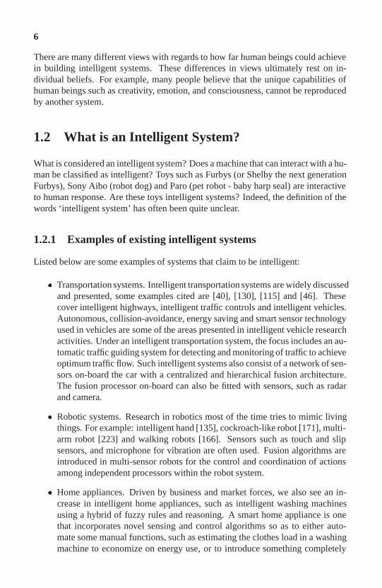
1.2.1 Examples of existing intelligent systems

Listed below are some examples of systems that claim to be intelligent:

� Transportation systems. Intelligent transportation systems are widely discussedand presented, some examples cited are [40], [130], [115] and [46]. Thesecover intelligent highways, intelligent traffic controls and intelligent vehicles.Autonomous, collision-avoidance, energy saving and smart sensor technologyused in vehicles are some of the areas presented in intelligent vehicle researchactivities. Under an intelligent transportation system, the focus includes an au-tomatic traffic guiding system for detecting and monitoring of traffic to achieveoptimum traffic flow. Such intelligent systems also consist of a network of sen-sors on-board the car with a centralized and hierarchical fusion architecture.The fusion processor on-board can also be fitted with sensors, such as radarand camera.

� Robotic systems. Research in robotics most of the time tries to mimic livingthings. For example: intelligent hand [135], cockroach-like robot [171], multi-arm robot [223] and walking robots [166]. Sensors such as touch and slipsensors, and microphone for vibration are often used. Fusion algorithms areintroduced in multi-sensor robots for the control and coordination of actionsamong independent processors within the robot system.

� Home appliances. Driven by business and market forces, we also see an in-crease in intelligent home appliances, such as intelligent washing machinesusing a hybrid of fuzzy rules and reasoning. A smart home appliance is onethat incorporates novel sensing and control algorithms so as to either auto-mate some manual functions, such as estimating the clothes load in a washingmachine to economize on energy use, or to introduce something completely

7

new, such as detecting boiling water on an electric cooktop [9]. The position-ing of an intelligent ventilator via acoustic feedback [162] for an intelligenthome system could reduce the noise from external sources, such as approach-ing aircraft or noisy vehicles. Algorithms considered for such intelligent homeappliances are: fuzzy logic, rule-based and knowledge-based controller.

� Diagnostic systems. These are intelligent online machine fault diagnostic sys-tems. These systems typically use algorithms such as data mining technique,neural network and rule-based reasoning or a combination of them. Data arenormally in textual form. An example of an intelligent diagnostic system canbe found in [80].

Beside the above listed examples, there are many more that have claimed to beintelligent systems in one way or another. And yet a lot more that do not use theword intelligent may also have a lot more intelligent capabilities than those claimed.

1.2.2 Learning from nature

There are groups of researchers that look to nature for inspiration on how to buildintelligent systems. Their research includes understanding and learning to engineerthe following:

� Swarm intelligence. Animals and insects are able to coordinate and groupthemselves for protection and to hunt for food. For example, ants are ableto coordinate with one another to carry heavy objects, a school of small fishis able to move as a large group for self-protection, bees are able to build abeehive in a cooperative way.

� Artificial immunology system. Our complex immune system is able to de-fend our body in a very intelligent way. Immune cells such as T-cells, areable to remember the pathogen (foreign objects such as viruses, bacteria, par-asites and other microbes) they have combated before, and are able to multiplythe ‘warrior’ cells very rapidly when they encounter the same pathogen again.Hence, learning from our immune system may provide some key answers to abetter way of building smart systems for particular applications, such as com-puter security systems. See Appendix A.5 for a short description of artificialimmunology systems.

� Intelligent sensory systems. Animals and insects have, in general, good sen-sory systems, which are effective and efficient. For examples, a dog’s noseis able to detect an object present even when the object is giving out a verylow odour signature, whereas the viper snake has a highly sensitive thermalsensing capability [118].

8

� Advanced locomotion. Animals and insects have highly advanced locomotionand control bio-mechanisms that enable the whole body or platform to movein a very stable and efficient manner within a specific environment.

1.2.3 How do we qualify a system as intelligent?

Dictionary definitions of intelligent include:

� Having or showing (usually a high degree of) understanding, clever, quicknessof mind.

� Endowed with the faculty of reason; having or showing highly developed men-tal faculties; well informed; knowing, aware (of).

� Having or showing powers of learning, reasoning, or understanding, especiallyto a high degree.

From the definitions and the examples given, the important attributes of an intel-ligent system would consist of words such as: learning, intuition, creativity, quick-ness of mind, clever, reasoning, understanding, autonomous behaviour or self gov-erning, adaptive, ability to self-organize, coordinate and possess knowledge. Otherthan human beings, no other living things or man-made machines could currentlyfulfil all the above requirements. However, if a system could fulfil a subset of theattributed words, the system would have to possess some form of intelligence (orsub-intelligence). This will include a system that could perform quickly with a cer-tain logical reasoning, and would be classified as ‘clever’ or ‘smart’.

One school of thought is that all intelligent systems must have the capability tolearn. In fact, the ability to learn dominated most of the studies in the late ’80s and’90s. Learning capabilities are often related to the study of artificial neural networks.Researchers unanimously agree that learning is an important attribute of intelligentsystems. However, that is not all what an intelligent system should have. Based onour human growth and development, we know that some of our functions are morethan just learnt. For example, the ability of a new born baby to suck the mother’sbreast milk is not taught but is innate. Hence, intelligent systems need to include adesigned element where knowledge already exist and not always need to be trainedor learnt.

The other school of thought is that biologically inspired algorithms, such asfuzzy logic, neural network and genetic algorithms, are non-optimal algorithms anddo not provide good solutions to a problem. Hence, it may not be the way to goin building intelligent systems. Mathematical modelling techniques or other statis-tical and probabilistic algorithms would be better than the so-called computationalintelligence algorithms.

However, it is clear that currently no single technique can solve all the attributeswe desire in building intelligent systems. Hence, a combination of various tech-

9

niques is the way to go.

Here we define an intelligent system as any system that could receive sensoryinformation and has the ability to process this information with a computationallyefficient and effective software, combined with one or more smart or intelligent algo-rithms (where the algorithm could be biologically inspired, mathematical modelled,statistical algorithms, etc.) for performing functions, such as control, managing re-sources, diagnostic and/or decision-making, to achieve multiple or single task/s orgoal/s.

The ultimate goal is for an intelligent system to be modelled after human intelli-gence. Figure 1.1 shows how a child in her early development would already possessthe ability to think and learn. Scientists are looking to the brain to enhance our cur-rent way of information processing. The ability to engineer such a system, that couldmatch the total functions of the brain in processing and controlling all the sensorysystems, plus managing the whole state of the body or platform in adapting and in-teracting with the dynamics of the environment, is a non-trivial task. In chapters 3and 5 the discussion on neural networks and cognitive intelligence are respectivelyrelated to the modelling and understanding of the brain.

Figure 1.1: A child can think and learn. The multiple sensory systems (suchas eyes and ears) will enable her to know the environment.

1.3 What Makes an Intelligent System

With the above definitions, the basic components of an intelligent system would be,but not limited to:

� sensor technology.

10

� computing technology.

� intelligent/smart algorithm.

� communication technology.

� platform.

This book, in particular, will concentrate on the intelligent or smart algorithmsused for developing intelligent systems and also focuses on fusion and control ofmultiple sensory system algorithms working in a network of fusion nodes.

The book does not present any work on communication technology and theplatforms that physically hold these technologies. However, it acknowledges thatthe development in both the communication and platform technology will certainlyplay an important role in building intelligent systems. Communication technologyhas been expanding rapidly. For example, optical transmission rates are hitting the100GHz and wireless communication, such as bluetooth 1, 802.11 2, ultrawideband3

and 3G/4G is continuously enhancing distributed networking structures. Hence, im-provements in communication technology will have a significant impact on buildingintelligent systems particularly in the arena of decentralized and distributed network-ing systems. Likewise, the platforms that carry these technologies have been improv-ing with the discovery of new material and new engineering designs. Our body isan example of the most beautifully designed platform where the human sensory sys-tems and the processing of sensory inputs from our brain enable us to function as anintelligent being.

1.3.1 How an intelligent system sees the world?

How does an intelligent system see the world or is aware of its environment? Sensortechnology plays an important role in helping an intelligent system see the world.This is well illustrated in our own sensory system. Without the eye, ear, skin, noseand tongue our brain will be totally useless even if it has the most powerful biologicalalgorithms.

Hence the growing importance of intelligent systems is in line with the increaseusage and improvement in sensory technology. Smart sensory technology that willmake sense of the information detected, and combines with intelligent algorithmsand fast processors will make the system better.

1Delivers data at speed of 700Kbps and range of about 10m.2802.11a delivers data at maximum speed of 54Mbps and range of about 30m.3Potential in delivering data up to 100Mbps and range of about 60m.

11

1.4 Challenges of Building Intelligent Systems

We will see more claims of intelligent systems research and development activitiesand even products with different applications. Each of these is indeed a part ofthe building blocks in making intelligent systems. They each have a synergy incontributing toward our quest of building the ultimate intelligent system. However,whether an intelligent system will ultimately match human creativity, flexibility, andhave consciousness is debatable.

This book discusses the challenges of building intelligent system into two parts.The first part will present the essential components that make an intelligent system.These are:

� Software design. Since the current building of intelligent systems relies heav-ily on software, a robust software design will play an important part. Softwareprogramming has moved from assembler and procedural style to object- andagent-oriented programming. The challenge of building good software to sup-port an intelligent system will be discussed. Agent-based software will also bediscussed and compared with object-oriented design.

� Biologically inspired algorithms. Intelligent systems will require smart soft-ware algorithms to provide all the support needed for control and decision-making in a dynamic and ever-changing environment. Many researchers havebeen involved in finding better and smarter algorithms for many centuries. To-day the challenge in this area continues, particularly in biologically inspiredalgorithms. These algorithms have a relationship to the way humans solveproblems and are seen as the right path in our quest to achieve the ultimateintelligent algorithms. Algorithms such as neural networks, genetic algorithmand fuzzy logic will be presented.

� Sensor systems. As discussed earlier, how the intelligent system sees the worldwill depend on the sensor systems built on it. Hence, knowing the types of sen-sor systems available and applying them appropriately will contribute towardbuilding robust intelligent systems.

The second part of the book will focus on data and information fusion, track-ing and sensor management. Fusion is one of the important aspects of an intelligentsystem. Fusion brings data from multiple sensors or multiple sources together toform useful information. High-level fusion processes also try to derive, predict andmake sense of information. This includes the process of understanding the situation,its impact and ultimately for implementing the decision-making process. Part of thehigh-level fusion, which is a larger part of the sensemaking process, resides in un-derstanding how our brain interprets information received from the sensory systems4. The understanding of information will form knowledge. How does an intelli-gent system understand the information to form a collection of knowledge and using

4Studies are on going in these areas at different research institutions. For example, the study on how

12

this knowledge with good judgment (or wisdom) for short-term and long-term needremains a challenging area of research.

the brain interprets the ears’ input has led to the discovery of virtual surrounding, in which two speakerssound like many more [129].

CHAPTER 2

Software Design for IntelligentSystems

Software is an essential engineering tool for intelligent system design.G. W. Ng

2.1 Introduction

In any software project, system analysis and design is an important process - moreso in the building of an intelligent system, which currently relies heavily on softwareprograms.

In this chapter, we aim to discuss the general software analysis and design issuesfor building intelligent software systems using UML (Unified Modelling Language).UML, in our opinion, is expressive enough to capture the design decisions requiredto design the software program used in intelligent systems. For example, there area lot of CASE (Computer Aided Software Engineering) tools developed for UMLthat could be used for building intelligent systems, such as expert systems. Fur-thermore, UML is extensible and very flexible, hence would be suitable for newertypes of smart software, such as intelligent software agents. Software design thatincludes the capability of agent technology may play an important role in futureintelligent systems. Hence, this chapter will also discuss software agent-based sys-tems, propose an agent-oriented software development methodology and discuss theobject-oriented versus agent-oriented software engineering issues.

This chapter is organized as follows: Section 2 presents the analysis and designusing UML. Section 3 presents the data structure and storage. Section 4 describeswhat is a software agent-based system. Section 5 proposes an agent-oriented soft-ware development methodology. Section 6 discusses on object versus agent-oriented

14

software engineering issues.

2.2 Analysis and Design Using UML

In any software project, software analysis and design phases are meant for definingthe architecture and help meet the needs of customers. They are achieved throughbuilding models. Models help us visualize a complex system under a controlledenvironment; it is a simplification of reality. There are a number of methodologiespushing software analysis and design. Of late, Object-Oriented Analysis and Design(OOAD) is particularly popular. Of these, Objectory (by Ivar Jacobson), the ObjectModelling Technique (OMT by James Rambaugh) and the Booch Methodology (byGrady Booch) are widely used and successful ones. More recently, a global effortpioneered by these 3 veterans, crystallized their expertize and experiences into astandard known as the Unified Modelling Language (UML) [37].

The UML is a standard language for visualizing, specifying, constructing anddocumenting a software product. It is methodology neutral and can be used to doc-ument a wide variety of software intelligent systems. A methodology will use thisexpressive language in producing a software blueprint. One example of such use isthe CommonKADS Methodology (a complete methodological framework for devel-oping knowledge-based systems). It uses UML notations.

2.2.1 Diagrams

Central to UML is a wide choice of diagrams, which are graphical presentations ofconnected elements and their inter-relationships. They are particularly useful for thevisualization and construction of software components. Table 2.1 shows the choiceof diagrams.

Note that the component and deployment diagrams exist in UML to help docu-ment the organization and dependencies of software components, and how the sys-tem is physically deployed. We find that they are not necessary in documentingagent-based systems per se but will be required to document the software implemen-tation of the system.

2.2.2 Relationships

There are basically 4 types of relationships in object-oriented modelling. These are:

� dependencies, which offer a loose coupling link within one class, using theservices of another.

� aggregation shows part-whole relationships.

15

Number Diagrams Descriptions1. Activity diagrams Activity diagrams show the flow of control within

a system or sub-system. They are particularlyeffective in showing concurrent activity. Usingswimlanes, ownership of an object can beclearly shown. Activity diagrams can be potentiallyused to show how various software agentsinteract concurrently with one another.

2. Sequence diagrams Sequence diagrams display how object interactsin a time sequence.

3. Collaboration diagrams Collaboration diagrams display objectinteractions organized around objects andtheir links to one another.

4. Class diagrams A class diagram is a collection of objectswith common structure, behaviour, relationshipand semantics. The class diagram is staticby nature. In agent-based systems, classescan be used to represent agents as well.Stereotypes can be used to markthe distinction for agent classes.

5. State transition A state transition diagram (STD) showsdiagrams the life history of a given class. It shows the

events that cause a class to transit fromone state to another. State transition diagramscan be nested; this allow us to effectivelymanage the complexity. In agent-basedsystems, the states of each agent couldbe represented by STD.

Table 2.1: Diagrams for software design.

� associations represent structural links among objects.

� generalization for the derivation of inheritance relationships.

2.2.2.1 Dependency

This is the relationship of one class depending on another class [37]. For example,when the object of a class appears in the argument list of a method of another class,the latter is using the former to do something. If the used class changes, there is ahigh chance that the user class is affected. So the user class depends on the usedclass. The example in Figure 2.1 shows that class A is dependent on class B toperform some services.

2.2.2.2 Aggregation

This relationship is useful to show that an object contains other objects, in what iswidely called the part-whole relationship. The container class, which is also calledthe owner class, typically creates and destroys the owned object. In Figure 2.2, the

16

B

A

Figure 2.1: Dependency relationship.

IAinNet class really is made up of an array of layers; each of these layers is itself anIAinObj. In UML notation, a diamond shape at the container end pointing towardsthe contained-object end shows an aggregation through reference. The multiplicityshown indicates that ‘1’ IAinNet object could contain 0 or more IAinObj objects.

The strong form of aggregation is known as composition. This is in cases whenthe owned object cannot be shared across different owners. Furthermore, the ownedobject forms an important component within the owner class. For example, a neuronclass is composed of an identification tag (could be an integer or string) and weights(could be floats or doubles) among other things. Figure 2.3 shows an example ofcomposition relationship.

2.2.2.3 Association

This is a structural relationship between 2 objects permitting the exchange of prede-fined messages between them (see Figure 2.4). The message flow can be unidirec-tional or bidirectional. For example, the Layer class could maintain a bidirectionalrelationship with a neuron class. This relationship offers a general relationship be-tween 2 classes, and is used whenever a class uses the services of another class. Anaggregation can be seen as an association.

2.2.2.4 Generalization

This is an inheritance relationship, where the derived class has all the characteristicsexposed by the parent classes. They are more widely called ‘is-a’ relationship. Forexample, an InputNeuron class may inherit from a Neuron class because the former‘is-a’ neuron with more specific roles serving within the input layer. In Figure 2.5,the class ‘Vehicle’ is a root class; derived from it are the car, bus or van classes. Thisrelationship is particularly useful for extending software capabilities. A class hier-

17

+<<virtual>> set(const int param, const int value):bool

+<<virtual>> get(cont IAinObj*, IAinObj*):bool

+<<virtual>> get(const int param, int &value):bool

+<<virtual>> IterateOneEpoch():bool

+<<virtual>> Propagate():bool

-Layers:IAinObj*

-NumLayers:int

+<<virtual>> set(const int param, IAinObj*):bool

+<<virtual>> get(const int param, IAinObj*):bool

IAinNet

IAinObj

AinLayer

-NumNeurons:int

-Neurons: AinNeuron*

+<<virtual>> set(const IAinObj*, IAinObj*):bool

0..*

1

Figure 2.2: Aggregation relationship.

archy almost always leverages on polymorphism to extend the behaviour of derivedclasses. In the example, the vehicle may provide a default drive method, which ispolymorphic (using keyword virtual). But in reality, driving a car may be slightlydifferent from driving a bus. So the drive method in the bus is defined so as to over-ride the default operation defined in the vehicle class. The power of a class hierarchyand polymorphism are further explored in a number of design pattern books.

2.3 Data Structure and Storage

Quite often, in building intelligent systems, the data structure and storage could becomplex. Traditionally, arrays and lists have been used for quick random or se-quential access, however, other data structures can be better explored. UML can beeffectively used in describing the software design of data structure and storage.

18

Sensor system

Locomotion system

Robot Data process system

Figure 2.3: Composition relationship.

2.3.1 Data structure

There are many data structures. A good software design generally has a good datastructure serving as the backbone. They are important because they ensure data areorganized properly. When the correct structure is used, the storage becomes scalable.Common structures are: lists, queues, stacks, trees, arrays, sets and maps.

In deciding the correct data structure to adopt in an intelligent application, onehas to study the following factors:

� How are data represented in the application? Certain data are, by nature, hier-archical. For example, in representing a graphical model in a 3D application,an obvious choice would be using a tree to organize the model.

� How should data be retrieved from the structure? In a neural network back-propagator application, trees seem a good choice. For example, we could havea layer as a branch, and under that branch we could have a number of nodes,each representing a neuron. The propagation is from one branch to the next,

19

B

A

Figure 2.4: Association between 2 classes.

in a lateral traversing manner. An alternative is to use a map data structure toorganize a neural network. A map relies on a key to look up some content. Anumber can identify the layer, and this is used as a key to obtain informationon a particular layer.

Usually, the choice of a data structure will depend on three issues:

� Ease of programming. Does the choice of a data structure make implementingthe system easier?

� Time efficiency. Various data structures offer different performance in termsof insertion, deletion and retrieval.

� Space efficiency. How much physical space a data structure occupies is alsoimportant. This is especially so in memory constrained systems.

2.4 What is a Software Agent-based System?

Rapid advances in information and communication technologies, notably Internetnetworking and wireless communications, are providing a new infrastructural andcommunications means to achieve higher levels of automation, flexibility and inte-gration in the development of distributed software applications. To mutually refineand exploit these technologies, multiagent systems (i.e. systems of multiple agents),according to Jennings et al. [112], are being advocated as a next generation modelsfor engineering complex, distributed systems [242, 113].

Agent-based systems could potentially represent a new way of analyzing, de-signing, and implementing complex software systems in a network-centric infras-tructure. It is claimed as a possible basis framework to bring together and extend thevast body of knowledge from artificial intelligence, computer and control sciences,operations research and related fields, such as economics and the social sciences

20

Car

Vehicle

is_a

is_a

is_a

Bus

Van

Figure 2.5: Generalisation relationship.

(reference Proceedings of the ICMAS’ 2000 1). Examples of potential agent-basedsystems are: personalized email filters, air-traffic control systems and command andcontrol systems. The potential applications of agents in many small and complexsystems are on hand. However, there are also concerns that certain aspects of agentsare being dangerously over-hyped and if not controlled, may suffer the same back-lashes as artificial intelligence (AI) in the 1980s.

2.4.1 What is an agent?

There is no universally agreed definition of the term agent. According to [243], anagent is defined as ‘a computer system that is situated in some environment and iscapable of autonomous action in this environment in order to meet its design ob-jectives’. In this chapter, we will mainly focus the discussion on software agents.Software agents can occupy many different environments, such as in the Internet orwithin a core local area network. The autonomous action of an agent is its abilityto control its own state and also can interact with humans, other systems or otheragents. Agents are flexible in the sense that they are [242]:

� responsive: agents should perceive their environment and respond in a timelyfashion to changes that occur in it;

1ICMAS: International Conference on MultiAgent Systems.

21

� proactive: agents should not simply act in response to their environment, theyshould be able to exhibit opportunistic, goal-directed behaviour and take theinitiative where appropriate;

� social: agents should be able to interact, when appropriate, with other artificialagents and humans in order to complete their own problem solving and to helpothers with their activities.

Hence, an agent that has all the attributes of these flexibility parameters, is alsoknown as an intelligent agent 2.

2.4.2 What is a multi-agent system?

Multi-agent systems refer to systems with multiple agents. In general, the study ofmulti-agent systems [236] involves three mutually dependent areas, namely: agentmodel and architecture, communication languages and interaction protocols. Anagent model refers to its internal architecture of integrated data structures and func-tionalities that should ideally support planning, reacting and learning, while a multi-agent architecture, in general, specifies an infrastructure for coordination or collabo-ration among the agents. Communication languages enable agents to describe theirmessages meaningfully for knowledge exchange, while interaction protocols enablethe agents to carry out structured exchanges of messages.

2.4.2.1 Multi-agent approach to distributed problem solving

When adopting an agent-based approach to distributed problem solving (DPS), it isclear that most problems will require multiple agents to represent the decentralized(or distributed) nature of the problem. Moreover, these agents will need to interactwith one another, to achieve their common or individual goals and to manage, so asto ensure a proper temporal order 3 among dependencies that may arise from beingsituated in a common environment [236, Chapter 2].

2.4.2.2 Multi-agent negotiation

One means of interaction is negotiation. By negotiation, we mean that agents workout, communicatively, an agreement that is acceptable by all agents. In distributedproblem solving, negotiation is one way that agents use in cooperation to solve theproblem. Generally, an automated means (or reasoning mechanism) of negotiation

2An intelligent agent is a software entity capable of flexible autonomous actions to meet their designobjectives (goals); autonomous in that it requires minimal or no human intervention and flexible (or in-telligent) in that each agent can react to perceived changes in a common environment, interact with otheragents when necessary, and take proactive steps towards its design goals agent [236, Chapter 1]

3In our view, what is proper is domain dependent, and is decidedly a subjective opinion of the agentdesigner/analyst.

22

for an agent can be implemented as a negotiation protocol within which a decision-making model (or logic) over the objects of negotiation resides.

In the literature on general negotiation frameworks, agents that can negotiatewith exact knowledge of each other’s cost and utility functions, or such knowledgelearnt in the initial step of interaction, have been proposed [131]. There are agentsthat negotiate using the unified negotiation protocol in worth-, state-, and task-drivendomains, where agents look for mutually beneficial deals to perform task distribution[198, 251]. In negotiation via argumentation (NVA), the agents negotiate by send-ing each other proposals and counter-proposals. In one NVA approach [132], theseproposals are accompanied by supporting arguments (explicit justifications) formu-lated as logical models. In another NVA approach [116], the distributed constraintsatisfaction problem (DCSP) algorithm [247] provides the computational model, ex-tended with the supporting arguments (accompanying the proposals) formulated aslocal constraints. In yet another approach [208], agents can conduct NVA in whichan agent sends over its inference rules to its neighbour to demonstrate the soundnessof its arguments. Finally, there are also negotiating agents that incorporate AI tech-niques (e.g. auction mechanisms and metaphor-based mechanisms that attempt tomimic human practical reasoning in some specific ways).

For a complete review of agent negotiation, readers may refer to Jennings et al.[112].

2.5 An Agent-Oriented Software Development Method-ology

Like object-oriented software development, we believe that an iterative approach todeveloping an agent-based software systems holds the best promise of successfullydeveloping such systems. An iterative approach allows important requirements ofthe system to be validated early and also serve to clarify unclear requirements. Theconcepts covered here do not represent a fully functional agent-based developmentmethodology but rather provide several suggestions on what to focus on during anal-ysis, design, coding and testing of multi-agent systems.

Typically, an iterative development has the following characteristics, as illus-trated in Figure 2.6.

In an iterative development approach, several phases of the system are createdto provide early feedback on the usability and performance of the system. Also,analysis, design, coding and testing can take place almost simultaneously. Note,however, that the effort expanded in analysis, design, coding or testing is different ineach time quantum. For example, during the initial development to the system, mostof the effort would focus on analysis. Towards the end of the development, most ofthe effort would be spent on testing. Various formal reviews are also planned duringthe development in order to track and monitor the progress of the project (i.e. we

23

: effort

Legend

Phases Iteration 1 Iteration 2 Iteration 3

Test ReadinessReview

DesignReviewReview

Analysis

System Integration &Testing

Design

Coding & Testing

Analysis

Time

1st runningsystem system

2nd runningsystem

Fully running

Figure 2.6: Example of an iterative approach to agent software development.

develop iteratively but manage it sequentially). These reviews also serve as ‘exitpoints’ to the project. For example, if the project cannot meet its expectation, theproject management team can choose to terminate the project.

Note that for more exploratory systems, a spiral development methodology canbe followed. Figure 2.7 shows a typical spiral development process. However, it willnot be discussed in this section.

In the discussion that follows, we will assume that the development of the agent-based system will be built on top of an agent-based infrastructure. Also, we will sug-gest appropriate UML diagrams suitable for capturing analysis and design decisions.

24

Project entrypoint axis

CustomerCommunication

CustomerEvaluation

Risk Analysis

Engineering

Construction & Release

Planning

Product Maintenance Projects

Product Enhancement Projects

New Product Development Projects

Concept Development Projects

Figure 2.7: Spiral development process [193].

2.5.1 Analysis

During the analysis phase, the system requirements of the system are analysed andtranslated to unambiguous specifications. Use-cases and interactions diagrams canbe used to capture these requirements. From the use-case description, agents can beidentified.

Having defined the use-case model, the roles of the system need to be found.Four types of roles need to be determined. These are:

� Responsibilities. This represents the dos and don’ts of that role.

� Permissions. This represents the type of information the role can access.

� Activities. This represents the tasks that a role performs without interactingwith other roles.

� Protocol. This refers to the specific pattern of interaction between roles.

After the roles have been identified and documented, the other important aspect is theinteractions between roles. Note that this is done when analysing the system require-ments after the agents are identified. This step examines how the agents collaborateto accomplish certain roles.

25

2.5.2 Design

In the design phase, the roles are mapped into agent types. Agent instances arecreated from each type. This is analogous to the classes and objects in the object-oriented world. The class diagram can be extended to be an agent diagram by stereo-typing the class as << agent >>. The same idea can be applied to agent instancesby extending the object representation. The next step is to develop the service model.This model captures how each agent fulfil its role. The collaboration diagram canbe extended to serve as a service model. Finally, the acquaintance model is created.This model captures the communication between agents. The interaction diagramcan be extended to represent the acquaintance model.

In detail design, we then decide what type of agents will best implement thesystem requirements. Here, the software designer will need to decide if an agentwill be a BDI (belief, desire, and intention), Reactive, Planning, Knowledge-basedor some other new user-defined agent architecture. In addition, in situations wherenon-agent based entities are required to be incorporated into the system, they shouldbe wrapped up as agents so that the entire design view of the system can be/havean agent-based view. Concepts on agent-based design pattern can also be appliedduring detail design.

2.5.3 Coding

In coding, the facilities provided by the agent-based infrastructure will be used tocode the system. For example, in the JACK agent infrastructure, the system is essen-tially Java codes. However, extensions incorporated into the Java language to provideagent-related facilities are used to implement agent behaviours and functions.

2.5.4 Testing

Testing of agent systems follows testing of traditional software system. The testcases should be derived from the use-case model. If certain agent behaviours need tobe verified, specific scenarios should be created to make verification possible. Thesystem can then be tested.

2.6 Object- and Agent-Oriented Software Engineer-ing Issues

Table 2.2 shows the functionality and feature differences between an object and anagent.

In most of the cases, agent-oriented designs are adapted from an existing object-oriented design methodology. Some even treat an agent as an active object. Agent-

26

Function/ Object Agent CommentsFeature

Method of By invoking other By requesting other Agents do itexecution objects. agents, it does not invoke because they

other agents. In other decide to do so.words, a request maynot be carried outas all agents haveautonomy to decide.

System goal Objects in a system In a multi-agent system,may share a common we cannot assume thatgoal. all agent will share

a common goal.Communication Communicate by Communication means is Object-oriented

message passing. more complicated than just communication structuremessage passing. Needs is well structured andcomplex protocols that studied. Agent-basedinvolves coordination and system protocols areinteraction with each other. still a research topic.

Encapsulation Objects encapsulate Agents encapsulatesome state and may some state and are notbe accessible to other accessible to other agentsobjects (unless it is It makes decisions aboutdeclared as private). what to do based onIt does not make this state withoutdecisions but simply direct interventionexecutes after the direct of human orintervention of human other agents.or other agents.

Behaviour Object-oriented design Agent-oriented designsfactor does not consider have to take into account

object flexible flexible behaviour such asbehaviour. reactive and pro-active

behaviour of an agent.Thread of Objects are quiescent Agents are continually Note that concurrencycontrol most of the time, active and typically are in object-oriented

becoming active only engaged in an infinite approach doeswhen another object loop of observing attempt to fufil somerequires their services. their environment, updating active role of an object

their internal state and but it does not captureselecting and executing the full autonomousan action. characteristics of an

agent.UML UML is defacto Some agent researchers Note that adapting

standard for are attempting to from UML may be oneobject-oriented adapt the UML notation of the best approachesapproaches. for agent-oriented for agent-oriented design.

approaches.

Table 2.2: Object versus agent software engineering issues

oriented software engineering is at an infancy stage of research and development.There are still many issues with regard to multi-agent system software engineering

27

design. Issues such as:

� Software design methodology of agents. These are currently under intensiveresearch. Adapting from UML may be one of the best approaches for agent-oriented design. However, it is also noted that the extension of UML for agent-oriented design would still need significant work particularly the problem ofthe relationship between agents and objects.

� Relationship of agents with other software paradigms. It is not clear how thedevelopment of agents systems will coexist with other software paradigms.This point also makes adapting the UML for agent-orientated software engi-neering important. Currently, most of the object-oriented software systems areanalysed and designed using UML.

� System robustness. With the massive number of agents dynamically interact-ing with one another in order to achieve their goals, it is not completely clearwhat happens to system stability and behaviour (chaotic behaviour). Someform of agent structure or organization may be necessary depending on theapplication domain.

CHAPTER 3

Biologically InspiredAlgorithms

Nature provides the main inspiration in designing intelligent systems.G. W. Ng

3.1 Introduction

Biologically inspired algorithms provide one of the essential tools in building in-telligent systems. As the name implies, these algorithms are developed or inventedthrough modelling and understanding of biological systems or nature’s own intelli-gence, such as the immune system, the human brain, the evolutionary of gene and thecollective intelligence of the insects or animals. The biologically inspired algorithmspresented here are genetic algorithms, neural networks and fuzzy logic. This chapterwill give an overview of these algorithms and also discuss some of the benefits anddrawbacks of each algorithm. Included in this chapter is a brief introduction on thetraditional expert system 1. Lastly, we also present the notion of fusing these algo-rithms to leverage on their strength and offset their weakness. The chapter providessufficient details to those engineers interested in utilizing these biologically inspiredalgorithms for various applications.

The chapter is arranged as follows: Section 2 presents the genetic algorithms.Section 3 presents the neural network. Section 4 presents the fuzzy logic algorithm.Section 5 presents the expert system. Section 6 briefly discusses the fusion of thevarious biologically inspired algorithms. Note that a brief description of the artificialimmunological system is presented in the appendix and the cooperative intelligenceis covered in chapter 8.

1Fuzzy logic, neural networks and genetic algorithms could also be viewed as part of the modernexpert system or knowledge-based information management system.

30

3.2 Evolutionary Computing

Evolutionary computing refers to algorithms that are based on the evolution of apopulation toward a solution of a certain problem. The population of possible so-lutions evolves from one generation to another, ultimately arriving at a satisfactorysolution of the problem. The collection of evolutionary computing algorithms canbe categorized into 4 methodologies, namely:

� Genetic algorithms.

� Genetic programming.

� Evolutionary strategies.

� Evolutionary programming.

These algorithms have been used successfully in many applications requiring theoptimization of multi-dimensional functions. The differences among the variousevolutionary computing algorithms are in their:

� Method of generating the evolving population; and

� Method of representing the population within the algorithm.

3.2.1 Biological inspiration

All living organisms consist of cells. In each cell there is the same set of chro-mosomes. Chromosomes are strings of DNA and serves as a model for the wholeorganism. DNA is shaped as a double spiral with linking bars, like a twisted ropeladder.

A chromosome consists of genes, blocks of DNA. Genes are the body’s chemicalinstructions. Each gene is an instruction to make a particular protein. Genes makeus unique, such as colour of eyes, hair, etc. Each gene has its own position in thechromosome. This position is called locus.

A complete set of genetic material (all the chromosomes) is called a genome.A particular set of genes in a genome is called a genotype. The genotype is, withlater development after birth, the base for the organism’s phenotype, its physical andmental characteristics, such as eye colour, intelligence, etc.

There are 46 chromosomes in each of our body cells, divided into 23 pairs. Onehalf of each chromosome pair came from the mother and the father.

During reproduction, genes from parents form, in some way, a whole new chro-mosome (also known as recombination or crossover). The newly created offspringcan then be mutated. Mutation means, that the elements of the DNA are slightlychanged. These changes are mainly caused by errors in copying genes from parents.

31

The fitness of an organism is measured by the success of the organism during itslife.

3.2.2 Historical perspectives

Evolutionary computing was inspired by Darwin’s theory of evolution. The idea ofevolutionary computing was introduced in the mid ’60s by Ingo Rechenberg in hiswork ‘Evolution Strategies’ [204]. Then the evolution strategies were evolution pro-grams with the objective of finding floating point solutions in optimization problems.Hence, floating point number representation was used.

In the late ’60s, Larry J. Fogel [79] and his colleagues developed what theycalled evolutionary programming. Evolutionary programming uses the selection ofthe fittest where the only structure modification allowed is the mutation process.There is no crossover and each point in the population represents the entire species.

Genetic algorithms (GAs) were developed by John Holland in 1975 [101]. In1992 John Koza of Stanford University used genetic algorithms to develop programsto perform certain tasks. He called his method ‘genetic programming’ (GP). HenceGP is a special implementation of GAs. LISP (LIst PRocessing) programs were thenused, because programs in this language can be expressed in the form of a ‘parsetree’, which is the concept the GA works on.

Of all the 4 methodologies, more work has been done with genetic algorithmsand their various applications. Hence, in the following subsection, we will presentthese genetic algorithms in more detail.

3.2.3 Genetic algorithms

GA is among the most popular and rapidly growing area in evolutionary computa-tion. GAs consider many points in the search space simultaneously, and have beenfound to provide rapid convergence to a near-optimum solution in many types ofproblems. GA will generally include the four fundamental genetic operations of:selection, crossover, mutation, and competition. GAs show much promise, but suf-fer from the problem of excessive complexity if used on problems that are too large.GAs are most appropriate for optimization-type problems and have been applied suc-cessfully in a number of applications such as control [88], weapon management andscheduling problems.

3.2.3.1 Introduction to GAs

GA starts with a set of solutions (represented by chromosomes) called a population.Solutions from one population are taken and used to form a new population. Thisis motivated by the hope that the new population will be better than the old one.Solutions which are selected to form new solutions (offspring) are selected according

32

to their fitness - the more suitable they are the more chances they have to reproduce.This reproduction circle (or evolving process) will be repeated continuously untilthe stop criteria are satisfied. The stop criteria could be that the number of evolvinggenerations or the expected performances are met.

The formation of GAs can be summarized by the following steps:

� Step 1 - Generate a random population of n chromosomes (suitable solutionsfor the problem).

� Step 2 - Evaluate the fitness f(x) of each chromosome x in the population.

� Step 3 - New population. Create a new population by repeating the followingsteps until the new population is completed.

� Step 4 - Selection. Select two parent chromosomes from a population accord-ing to their fitness (the better the fitness, the bigger the chance to be selected).

� Step 5 - Crossover. With a crossover probability cross over the parents to forma new offspring (children). If no crossover was performed, the offspring is anexact copy of parents.

� Step 6 - Mutation. With a mutation probability mutate new offspring at eachlocus (position in chromosome).

� Step 7 - Accepting. Place new offspring in a new population.

� Step 8 - Replace. Use new generated population for a further run of the algo-rithm.

� Step 9 - Test. If the stop criteria is met, stop, and return the best solution incurrent population, else go to step 2.

The basic GA steps are very general. There are many variations or modificationto these general GA steps in solving different problems.

The fundamental questions are:

� What types of encoding are suitable to create chromosomes? Or how to repre-sent the population?

� What operators are effective for crossover and mutation?

� How to select the parents for crossover?

� How to formulate the fitness evaluation function?

All the above questions could be answered in many different ways. For example,there are many possible ways of encoding the chromosomes, typically used are bi-nary strings (this will be illustrated in the next subsection of this chapter). However,depending on the problem to be solved, integers or real numbers could also be used.

33

3.2.3.2 Operator

As you can see from the genetic algorithm outline, the crossover and mutation are themost important parts of the genetic algorithm. The performance is influenced mainlyby these two operators. Before we explain more about crossover and mutation, someinformation about encoding the chromosomes is necessary.

How do we encode the chromosome? The chromosome should in some waycontain information about the solution that it represents. The chromosomes encodedby a binary string (commonly used) could then look like this:

Chromosome 1 1001100100110110Chromosome 2 1001111000011110

Each chromosome has one binary string. Each bit in this string can representsome characteristic of the solution. Or the whole string can represent a number.

Crossover

After we have decided what encoding we will use, we can implement the crossover.Crossover selects genes from parent chromosomes and creates a new offspring. Thesimplest way is to choose randomly some crossover point where everything beforethis point is copied from a first parent, and then everything after the crossover pointis copied from the second parent.

Crossover can then look like this (where ‘ — ’ is the crossover point):

Chromosome 1 10011 — 00100110110Chromosome 2 10011 — 11000011110

Offspring 1 10011 — 11000011110Offspring 2 10011 — 00100110110

There are other ways on how to make a crossover. For example, we can choosemore crossover points. Specific crossovers made for a specific problem can improveperformance of the genetic algorithm.

Mutation

After a crossover is performed, mutation takes place. The mutation process helpsprevent solutions in the population from falling into a local optimum. Mutationchanges randomly the new offspring. For binary encoding we can switch a fewrandomly - chosen bits from 1 to 0 or from 0 to 1. Mutation can then be as follow:

34

Original offspring 1 1001111000011110Original offspring 2 1001100100110110

Mutated offspring 1 1000111000011110Mutated offspring 2 1001101100110110

Mutation means different things for different data types. In the above example,which uses a binary string, mutation involves flipping the bits in the string witha given probability. A typical mutator for a tree, on the other hand, would swapsubtrees with a given probability.

The mutation depends on the encoding as well as the crossover. For example,when we are encoding permutations, mutation could be exchanging two genes.

3.2.3.3 Parameters of GAs

Here, we cover three GA parameters namely: the crossover probability, mutationprobability and the population size.

Crossover and Mutation Probability

There are two basic parameters of GAs - crossover probability and mutation prob-ability. Crossover probability determines how often crossover will be performed.If there is no crossover, the offspring is an exact copy of the parents. If there isa crossover, the offspring is made from parts of the parents’ chromosome. If thecrossover probability is 100%, then all offsprings are made by the crossover. If itis 0%, the whole new generation is made from exact copies of chromosomes fromthe old population (but this does not mean that the new generation is the same!).Crossover is made in the hope that new chromosomes will have good parts of oldchromosomes and maybe the new chromosomes will be better. However, it is goodto leave some part of the population to survive into the next generation.

Mutation probability says how often the gene in the chromosome will mutate.If there is no mutation, the offspring is taken (or copied) after the crossover withoutany change. If mutation is performed, part of the chromosome is changed. If themutation probability is 100%, the whole chromosome is changed - if it is 0%, nothingis changed. Mutation is made to prevent GAs from falling into local extreme, but thisshould not occur very often because then the GAs will in fact change to a randomsearch.

Population size

Population size determines how many chromosomes are in a population (in one gen-eration). If there are too few chromosomes, GAs have fewer possibilities to performa crossover and only a small part of the search space is explored. On the other hand,

35

if there are too many chromosomes, the GA slows down. Research shows that af-ter some limit values (which depend mainly on encoding and the problem), it is notuseful to increase the population size, because it does not solve the problem anyfaster.

3.2.3.4 Selection

As you already know from the GA outline, chromosomes are selected from the pop-ulation to be parents for crossover and mutation. The problem is how to select thesechromosomes. According to Darwin’s evolution theory the best ones should surviveand create new offsprings. There are many methods of selecting the best chromo-somes, for example, roulette wheel selection, Boltzman selection, tournament selec-tion, rank selection, steady state selection, elitism and others. Two of them will bedescribed in this section.

Roulette Wheel Selection

The Roulette wheel selection method provides a mechanism where the parents areselected according to their fitness. The better the chromosomes are, the more chancesthey will be selected. Imagine a roulette wheel where all the chromosomes in thepopulation are placed. The space the chromosomes occupy in the wheel determinehow good are the chromosomes. The ‘goodness’ of the chromosome is measured bythe probability of the reproduction. The probability of the reproduction is computedby P (Xi) =

f(Xi)Ppj=1 f(Xj )

where Xi is the i chromosomes.

Elitism

When creating a new population by crossover and mutation, we run the risk that wewill lose the best chromosome. The elitism method overcomes this by keeping thebest-fit chromosome. The method transfers the best chromosome (or a few best chro-mosomes) to the new population. The rest of the steps are carried out as discussed.Elitism can very rapidly increase the performance of the GA, because it preventslosing the best found solution.

3.2.3.5 Further information on crossover and mutation operators

Crossover and mutation are two basic operators of GAs. The performance of GAsis affected by how the operators are implemented. Listed below are some possibleways of how a crossover and mutation operator could be performed:

36

Crossover

1. Single point crossover - one crossover point is selected. Example: 10010111+ 11010010 = 10010010

2. Two point crossover - where two crossover points are selected, the binarystring from the beginning of the chromosome to the first crossover point iscopied from one parent, the part from the first to the second crossover point iscopied from the second parent and the rest is copied from the first parent.

3. Uniform crossover - bits are randomly copied from the first or from the secondparent. Example: 11001011 + 11011101 = 11011111

4. Arithmetic crossover - some arithmetic operation is performed to make a newoffspring. Example: 11001011 + 11011111 = 11001001 (AND)

Mutation

1. Bit inversion - selected bits are inverted. Example 11001001 = 10001001

2. Add a small number (for real value encoding) - the selected values are added(or subtracted) with a small number. Example: (1.29 5.68 2.86 4.11 5.55) =(1.29 5.68 2.73 4.22 5.55).

Some drawbacks of genetic algorithms

The first drawback of a GA is that it has no concept of an ‘optimal solution’. Itcannot be proven that the solution is optimal. The second drawback of the GA is thatit does not address when to stop evolving in terms of the length of time, number ofiterations and the population size you would like to explore during the search for thebest solution.

3.3 Neural Networks


The human brain is made up of more than 100 billion nerve cells. Each of thesenerve cells is known as a neuron. Neurons are spider-shaped cells (Figure 3.1) andhave three basic elements namely: the dendrites, the soma and the axon.

The dendrites receive signals from other neurons. These signals are electricimpulses that are transmitted across a synaptic gap by means of a chemical process.

The soma, or cell body, sums the incoming signals. When a sufficient input isreceived, the cell fires; that is, it transmits a signal over its axon to other neurons.

37

Figure 3.1: The nerve cell.

An axon is the winding tail of the neuron. Its length could be up to 1 meterlong. Fatty covering called a myelin sheath often surrounds axons. Myelin acts likeinsulation around an electric wire and helps speed nerve messages. Axons of oneneuron are linked to the dendrites of other neurons. Using this link, each neuronis connected to as many as 25,000 other neurons. The brain has trillions of theseinterconnections and different pathways for nerve signals to flow through.

The study of artificial neural networks is trying to model or mimic the biologicalinterconnections of the neurons.

3.3.2 Historical perspective

The concept of using neural networks (NNs) came into existence in the mid 1940s.In 1943, McCulloch and Pitts designed boolean logic by combining many simpleunits. The weights on a McCulloch-Pitts network are set so that each unit performsa particular logic function [155]. These logic functions are combined to produce thedesired network output. The McCulloch-Pitts network was generally regarded as thefirst NN. Then came Hebb [96], a psychologist at McGill University, who published abiologically plausible learning rule. Hebb’s work formed some important theoreticalaspects of the learning algorithms for NNs. In around 1954, Minsky introduced thereinforcement learning (RL), a term borrowed from animal learning literature. RLwas also independently introduced and applied in control theory by Waltz [228] andMichie [159]. In 1957, Bellman created dynamic programming (DP). DP providesan efficient mechanism for sequential-decision making which was found to be usefulin reinforcement learning in the 90s. In 1958, Frank Rosenblatt coined the termperceptron, which became a popular word used in the NNs for the 80s and 90s.

38

Perceptron is a single layer NN, hence it has no hidden layer.

Then came the least mean square (LMS) algorithm, also known as the Widrow-Hoff rule or delta rule, developed by Bernard Widrow and Marcian Hoff of StanfordUniversity. This algorithm was applied to a simple adaptive linear neuron (Adaline).

In the 70s, much attention was directed towards the field of artificial intelligence(AI). This shift in focus was partly due to the Minsky and Papert analysis whichchallenged the incipient neural theory by establishing criteria for what a particularnetwork could and could not do [52]. However, during these silent years, threepioneering works on NNs were done. These are listed below:

� Werbos [237] proposed the concept of backpropagation (BP) for forecastinganalysis.

� Grossberg [89] proposed a learning algorithm for the instar and outstar net-work configuration.

� Willshaw and Ver Der Malsburg [241] proposed a self-organizing feature mapon biological grounds to explain the problem of retinotopic mapping from theretina to the visual cortex.

It is interesting to observe that what happened in the 70s is repeated in the early80s by independent researchers. To begin with, we have Hopfield [102], who intro-duced the network architecture that has come to be known as the Hopfield network.The Hopfield network has great similarity to the ‘Brain-State-in-a-Box’ (BSB). Boththe networks are fully interconnected. Therefore, each unit is connected to everyother unit. The only difference is that BSB network has self-connections while theHopfield network does not have. At about the same time, Kohonen independentlyintroduced self-organizing feature mapping to capture the essential features of com-putational maps in the brain [123]. The Kohonen network is quite similar to the Will-shaw and Ver Der Malsburg self-organizing feature map. In the same year, Parker[182] independently discussed the BP algorithm. The BP algorithm, sometimes alsoknown as the generalized delta learning rule, was later reinvented and made popularby Rumelhart and McClelland in 1986 [202].

In the mid 80s, there was the development of thermodynamic models. Twoexamples of such models are harmony theory [211] and the Boltzmann machine.Ackley et al. [1] developed a learning rule using the Boltzmann machine. Theseapproaches have much in common. Both employ binary units whose values aredetermined probabilistically according to the Boltzmann equation.

A sudden upsurge of interest in NNs occurred after the publication of the book byRumelhart and McClelland [202]. The following year, the IEEE conducted the firstconference on neural networks. The International Neural Network Society (INNS)was also formed in the same year and the first issue of its journal, Neural Networks,appeared early in 1988. Thereafter the IEEE Control Systems Magazine devoted atleast three special issues to the use of NNs for control (April 1988, 1990 and 1992).

39

In the late 80s to early 90s, we have seen many developments in NNs. New NNstructures such as: the radial basis function network [41], bidirectional associativememories [126], B-splines network [164], digital neurocomputer [97], functional-link networks [181], knapsack packing networks [98] and wavelet networks [248]were proposed. Different combinations of network topologies to improve the rep-resentational structure, such as recurrent backpropagation which combines feedbackand feedforward topologies, were explored [3, 188, 240].

During this period a number of papers were published seeking to improve the BPalgorithm. For examples, backpropagation with momentum, delta-bar-delta [110],Quickprop [76], decoupled momentum [160] and adaptive backpropagation [183].The number of books published on NNs have also increased manyfold [22, 36, 27,45, 52, 65, 69, 84, 99, 77, 125, 95, 158, 172, 214, 219, 224, 232, 231, 244].

3.3.3 Neural network structures

3.3.3.1 Basic units

The basic processing element of NNs is often called a neuron (analogy with neu-rophysiology), unit, node, or sometimes cell. In this book, we will simply call thisbasic element a unit. Each unit has multiple inputs and a single output, as shown inFigure 3.2. Many of these basic processing elements may be considered to have twobasic components, namely the summer and the activation function.

X

X

X

X

1

1

2

3

q

ΣS O

f(S)

Figure 3.2: The basic elements of neural networks.

Summer

The summer (or also known as adder) sums up the input signals. The respective inputsignals, before being summed up by the summer, are weighted by the respective linkor synapses of the neuron. In other ways, the summer is doing a linear combinationof the weighted input signals.

40

Activation function

The activation function transforms the summer output to neuron output through anon-linear function. This transformation squashes (or limits) the amplitude of theoutput neuron to some finite values. There are a number of different activation func-tions. These activation functions could be classified as:

1. Differentiable/non-differentiable.

2. Pulse-like/step-like.

3. Positive/zero-mean.

Each of the above classifications are briefly described and examples given:

� Classification 1 distinguishes smooth from sharp functions. Smooth functionsare needed for some adaptation algorithms, such as backpropagation, whereasdiscontinuous functions are needed to give a true binary output. Examplesof smooth functions are: sigmoid function, hyperbolic tangent function andradial basis function (RBF). An example of a sharp function is the hard-limiteror threshold transfer function.

� Classification 2 distinguishes functions which only have a significant outputvalue for inputs near to zero from functions which only change significantlyaround zero. For examples, the RBF can be pulse-like and the hard-limiterstep-like.

� Classification 3 refers to step-like functions. Positive functions change from 0at �1 to 1 at 1; zero-mean changes from -1 at �1 to 1 at 1. The sigmoidfunction is a positive function and the hyperbolic tangent function is zero-mean. A hard-limiter function can either be positive or zero-mean functiondepending on how the limit is defined.

There are cases where the network topology consists of rule units; each of theunits corresponds to a specific fuzzy rule. Therefore, all the units form a generalfuzzy rule [218].

3.3.3.2 Network topology

There are basically two network topologies, namely feedforward neural network(FNN) and recurrent neural network (RNN). Figure 3.3 shows the basic structures ofFNN and RNN. Both of these networks can have either fully connected or partiallyconnected structures; and either single layer or multilayer. A single layer neuralnetwork (SNN) has no hidden layer, hence it has only an input layer and an outputlayer (sometimes also known as a two layers network). A multilayer neural network(MNN) has at least one hidden layer.

41

Feedforward Neural Network

Recurrent Neural Network

Inputs Outputs

neuron or unit

OutputsInputs

Figure 3.3: Difference between feedforward and recurrent neural networks.

Feedforward neural networks

A FNN is completely feedforward with no past state of the network feeding back toany of its units. FNN is classified as fully connected, if every unit in the layer ofthe network is connected to every other unit in the adjacent forward layer. However,if some of the communication links (or sometimes called synaptic connections) aremissing from the network, we say that the network is partially connected.

FNN is static mapping, so theoretically it is not feasible to control or identifydynamic systems. To extend this essentially steady state mapping to the dynamicdomain would mean to adopt an approach similar to the linear theory of ARMA(autoregression moving average) modelling. Here, a time series of past real plantinputs and outputs values are used as inputs to the FNN with the help of tappeddelay lines (TDL). The nonlinear dynamic plant in discrete time is

yp(k) = f(yp(k � 1); : : : ; yp(k � ny); u(k � 2); : : : ; u(k � nu)) (3.1)

where f(:) is the unknown nonlinear function, yp is the plant output, u is the controlsignal, ny and nu are the number of past outputs and inputs of the plant dependingon the plant order. To represent this plant, the NN model is fed with the past outputand input values of the plant as follows (see Figure 3.4):

ym(k) = NN(yp(k � 1); : : : ; yp(k � ny); u(k � 2); : : : ; u(k � nu)) (3.2)

42

This assumes that the plant order is known and its states are measurable.

According to Levin [140], to represent the dynamics of the system sufficiently,at least l past measurements of the real plant output and input feeding back to theFNN input are required, where l � ny + nu + 1.

The assumptions that all the plant outputs and inputs are measurable and avail-able for feedback is sometimes unrealistic; for instance some plant outputs may notbe accessible for sensors (such as rotor currents in a squirrel cage induction motor)or the required sensors may be too expensive or unreliable. Hence for such a system,the FNN may not be suitable and a RNN may be preferred. This will be discussed inthe next subsection.

Recurrent neural networks

A RNN distinguishes itself from a FNN in that it has at least one feedback loop. Itis claimed that the presence of feedback loops has a profound impact on the learningcapability of the network and on its performance [188, 185, 240, 133]. In the senseof control theory, the feedback loop makes a RNN a nonlinear dynamic system. Thefeedback loops commonly involve unit delays if dealing with discrete-time systems,or integrators in the continuous-time case. RNNs may be preferred to FNNs when:

� The measured plant outputs are highly corrupted by noise.

� The dynamics of the nonlinear process are complex and unknown.

� Direct state feedback is impossible and only partial measurement is availablefrom the plant.

There are apparently many structures of RNN using different combinations offeeding back the states to the units in each layer. In RNN, the more general isthe structure, therefore more feedback interconnections (or fully-connected recurrentneural network (FRNN)), the ‘richer’ is the dynamic representation. Hence, FRNNsare sometimes said to have global dynamic representation. The more general typesare the Jordan, Elman and Williams-Zipser networks. In a Jordan network, the pastoutput values of the network are fed back into the hidden units or the input layer. Inthe Elman network, the past values of the hidden units are fed back into themselves[75, 134].

One of the problems in using FRNNs is the stability issue [127, 222]. Here, thetopic is addressed by looking at the recurrent weights. FRNNs are normally trainedby using the BP algorithm. To improve the stability of FRNNs, it is proposed herethat the total dynamic feeding back has to be less than 1. Hence, by considering theFRNN of an Elman network trained by a BP algorithm,

0 <

pXj=1

wrij(k)f0

hj(Shj(k � 1)) < 1 (3.3)

43

where wrij(k) is the recurrent weight at time step k, p is the number of hidden unitsand fhj is the activation function of the jth hidden unit, where usually the sigmoid orhyperbolic tangent function is used. Since j f 0

hj;max j = 1, wrij has to be boundedas follows to ensure FRNN stability:

0 < wrij <1

p(3.4)

Single layer and multilayer neural networks

NNs in feedforward or recurrent structures can be connected in a single layer neuralnetworks (SNNs) or multilayer neural networks (MNNs). The radial basis functionnetwork (RBFN), B-spline network, functional-link network (FLN), CMAC, latticeassociative memory network, Adaline and perceptron are feedforward SNNs. Mul-tilayer perceptron (MLP) is a feedforward MNN. Boltzmann machine and bidirec-tional associative memories (BAM) could be classified as recurrent MNNs. Adaptiveresonance theory (ART), Kohonen and Hopfield networks could be classified as re-current SNNs.

Both the MNN and SNN are universal approximators. A MNN with one hiddenlayer and sufficient hidden units can approximate any arbitrary nonlinear function[86, 62, 103, 190, 104, 87, 114]. Although a MNN with two hidden layers may givea better approximation for some specific problems [213], DeVilliers and Barnard[68] have demonstrated that a MNN with 2 hidden layers are more prone to fall intolocal minima.

A SNN is sometimes categorized as locally generalizing [6]. The network isconsidered local since only a small subset of adaptable parameters can potentiallyaffect the network output in a local region of the input space. The MNN is some-times categorized as globally generalizing. This is because one or more adaptableparameters in the network can potentially affect the network output at every point inthe input space.

3.3.4 Learning algorithms

Basically, there are three types of neural network learning algorithms. These are:supervized learning, reinforcement learning and unsupervized learning.

3.3.4.1 Supervized learning

Early learning algorithms

The early learning algorithms are designed for single layer neural networks. Theyare generally more limited in their applicability. Some of the early algorithms areperceptron learning, LMS learning and Grossberg learning.

44

Perceptron learning

Rosenblatt’s single layer perceptron is trained as follows:

1. Randomly initialize all the networks weights.

2. Apply the inputs x and calculate the sum of each unitS j(k) =Pq

i=1 xi(k)wij(k).

3. The outputs from each unit are

Oj(k) =

�1 Sj(k) > threshold0 otherwise

4. Compute the errors ej(k) = Odj(k) � Oj(k) where Odj(k) is the knowndesired output value.

5. Update each weight as wij(k + 1) = wij(k) + �xi(k)ej(k).

6. Repeat steps 2 to 4 until the errors reach the satisfactory level.

LMS or Widrow-Hoff learning

The least mean square (LMS) learning algorithm, sometimes known as Widrow-Hoff learning or delta rule, is quite similar to the perceptron learning algorithm. Thedifferences are:

1. The error is based on the sum of inputs to the unit S rather than the outputbinary value from the unit O. Therefore

ej(k) = Odj(k)� Sj(k)

2. The linear sum of the inputs S are passed through bipolar sigmoidal functions,which produces the output +1 or -1, depending on the polarity of the sum.

Grossberg learning

The Grossberg learning algorithm, sometimes known as instar and outstar training,is updated as follows [231]:

wi(k + 1) = wi(k) + �[xi(k)� wi(k)]

where xi could be the desired input values (instar training) or the desired outputvalues (outstar training) depending on the network structure.

45

3.3.4.2 First order gradient methods

Backpropagation

The backpropagation (BP) algorithm is the most well known and widely used amongother learning algorithms described in the literature. It is based on steepest-descenttechniques extended to each of the layer in the network by the chain rule. Hence,the algorithm computes the partial derivative @E(k)

@W (k�1) , of the error function withrespect to the weights. Suppose we want to model a nonlinear plant using a NN

y

e

NN m

Plantu

TDL

TDL

TDL

ym

p

Figure 3.4: Multilayer feedforward neural network modelling a nonlineardynamic plant.

(see Figure 3.4). The NN model output is ym. The error function is defined asE(k) = 1

2 [yp(k)�ym(k)]2 where yp is the plant output and em(k) = yp(k)�ym(k).The objective is to minimize the error functionE(k) by taking the error gradient withrespect to the parameters or weight vector, say W , that is to be adapted. The weightsare then updated by using

W (k) =W (k � 1) + �(� @E(k)

@W (k � 1)) (3.5)

where � is the learning rate and

@E(k)

@W (k � 1)= �em(k) @ym(k)

@W (k � 1)

46

= �em(k) @Oo(k)

@W (k � 1)

The network output is Oo(k) = ym(k), in this example.

This standard BP algorithm is simple to implement and computationally lesscomplex than other modified forms of BP algorithms. Nevertheless, it has somedisadvantages such as:

1. Slow convergence speed.

2. Sensitivity to initial conditions [124].

3. Trapping in local minima.

4. Instability if learning rate is too large.

Despite the above disadvantages, it is popularly used. There are numerous extensionsto improve the BP algorithm. Some of the more common techniques are as follows.

Backpropagation with momentum

The basic improvement to a BP algorithm is to introduce a momentum term in theweights updating equation [201]. Hence, the weights updated by backpropagationwith momentum (BPM) are

W (k) =W (k � 1) + (�� @E(k)

@W (k � 1)) + ��W (k � 1) (3.6)

where the momentum factor � is commonly selected between 0 < � < 1. Addingthe momentum term improves the convergence speed and helps the network frombeing trapped in a local minimum.

A modification to equation (3.6), such as

W (k) =W (k � 1) + (�� @E(k)

@W (k � 1)) + ��W (k � 1) + ��W (k � 2) (3.7)

was proposed by Nagata et al. [168], where � is a constant value decided by theuser. Nagata et al. [168] claimed that the � term reduces the possibility of thenetwork being trapped in the local minimum. However, this seems to be repeatingthe role of the � term. Hence, the advantage of adding the � term is not clear at themoment.

Delta-bar-delta

The delta-bar-delta (DBD) learning rules use an adaptive learning rate to speed upthe convergence. The adaptive learning rate adopted is based on a local optimization

47

method. It is an improvement from the delta-delta learning rule. This techniqueuses gradient descent for the search direction, and then applies individual step sizesfor each weight. This means that the actual direction taken in weight space is notnecessarily along the line of the steepest gradient [110].

If the weight updates between consecutive iterations are in opposite directions,the step size is decreased, otherwise it is increased. This is prompted by the idea thatif the weight changes are oscillating, the minimum is between the oscillations, anda smaller step size might find that minimum. The step size may be increased againonce the error has stopped oscillating.

Let �ij(k) denote the learning rate for the weight w ij(k), then

�ij(k + 1) = �ij(k) + ��ij(k) (3.8)

and ��ij(k) is as follows:

��ij(k) =

8<:

� � ij(k � 1) ij(k) > 0��ij(k) � ij(k � 1) ij(k) < 00 otherwise

(3.9)

where ij(k) =@E(k)@wij

and � ij(k) = (1 � ") ij(k � 1) + " � ij(k � 1). The " isa positive constant. �; � and " are parameters specified by the user. The quantity� ij(k) is basically an exponentially decaying trace of gradient values. When the �and � are set to zero, the learning rates assume a constant value as in a standard BPalgorithm.

Results cited by Jacobs [110] indicate that using momentum along with the DBDalgorithm can enhance performance considerably. However, it can also make thesearch diverge wildly; especially if � is moderately large. The reason is that mo-mentum ‘magnifies’ learning rate increments and quickly leads to inordinately largelearning steps. One possible solution is to keep the � factor very small, but this caneasily lead to slow increase in � and little speedup.

Simulations have also shown that the DBD algorithm is very sensitive to smallvariations in the value of its parameters, especially �. To overcome these problemsthe decoupled momentum is suggested.

Second order gradient methods

Second order gradient methods make use of second derivatives of the error in theweight space. The key to second order gradient methods is the Hessian matrix H .The Hessian matrix is a matrix of second derivatives ofE with respect to the weightsW .

H(k) =@2E(k)

@W (k � 1)2(3.10)

48

The Hessian matrix contains information about how the gradient changes in differentdirections in weight space. It answers the question: ‘How does the gradient changeif I move off from this point in that direction?’.

Newton

The Newton method weights update are [58]

W (k) =W (k � 1) + �[H(k)]�1@E(k)

@W (k � 1)(3.11)

However, the Newton method is not commonly used because calculating the Hessianmatrix is computationally expensive. Furthermore an Hessian matrix may not bepositive definite at every point in the error surface. To overcome the problem, severalmethods have being proposed to approximate the Hessian matrix.

Gauss-Newton

The Gauss-Newton method produces an n� n matrix which is an approximation tothe Hessian matrix, having elements represented by

H(k) = T (k) (k) (3.12)

where (k) = @e(k)@W (k�1) [145]. However, the Gauss-Newton method may still have

ill-conditioning if H(k) is close to or is singular.

Levenberg-Marquardt

The Levenberg-Marquardt (LM) method overcomes this difficulty by including anadditional term � which is added to the Gauss-Newton approximation of the Hessianmatrix giving

H(k) = T (k) (k) + �I (3.13)

where � is a small positive value and I is the identity matrix. � could also be madeadaptive by having

� =

�� Ec(k) > Ec(k � 1)�� Ec(k) < Ec(k � 1)

where � is a value decided by the user. Notice that when � is large, the algorithmbecomes a backpropagation algorithm with learning rate 1

� , and when � is small, thealgorithm becomes Gauss-Newton.

49

Quickprop

Fahlman [76] proposed the Quickprop method using heuristics based loosely on theNewton method. Fahlman highlighted that the Quickprop algorithm is based on tworisky assumptions:

� The error vs weight curve for each weight can be approximated by a parabola.

� The change in the shape of the error curve, as seen by each weight, is notaffected by all the other weights that are changing at the same time.

Hence, Quickprop implicitly assumes that the Hessian matrix is diagonal. Theweights update of the Quickprop algorithm, �W (k), is as follows:

�W (k) =(k)

(k � 1)�(k)�W (k � 1)

where (k) = @E(k)@W (k�1) . Fahlman claimed that when applied iteratively Quickprop

is very efficient.

Conjugate gradient decent

The idea behind conjugate gradient decent (CGD) is to choose search directions thatcomplement one another. This is to avoid the possibility of ‘undoing’ the minimiza-tion of previous iterations, by choosing appropriate search directions.

Assume that the error surface is quadratic in weight space.

E(k) = CTW (k � 1) +1

2W T (k � 1)H(k)W (k � 1) (3.14)

where C is a constant matrix and H is a Hessian matrix, constant throughout theweight space. The search direction at iteration k is denoted by v(k).

Set the first direction, v(1), to minus the gradient � @E(1)@W (0) . Set subsequent di-

rections using:

v(k) = � @E(k)

@W (k � 1)+ �(k)v(k � 1) (3.15)

where �(k) is a scalar value like an adaptive momentum term. � may be defined ina number of ways, each of which produces conjugate directions. The Polak-Ribiererule for � is [99]

�(k) =[(k)�(k � 1)]T [(k)]

[(k � 1)]T [(k � 1)](3.16)

50

The Hestenes-Stiefel rule for � is [163]

�(k) =[(k � 1)�(k)]T [(k)]

v(k)T [(k � 1)](3.17)

CGD will reach the minimum of a quadratic error surface in, at most, as manysteps as there are dimensions of the weight space. For non-quadratic error surfaces,the minimum may not have been reached after this number of steps. Instead, thealgorithm is restarted by setting � to zero for a step, and the procedure continues asbefore.

Conjugate gradients give only a search direction, not a step size. Furthermore,the power of conjugate gradients is only apparent if the error is minimized along thecurrent search direction.

3.3.4.3 Reinforcement learning

Thus far, we have assumed that the correct ‘target’ or the desired output values areknown for each time step or each input pattern. But, in some situations, there isless detailed information available. In the extreme case there is only a single bit ofinformation, saying whether the output is right or wrong. Reinforcement learning(RL) procedures are applicable to this extreme case. Hence, RL is sometimes called‘learning with a critic’. One advantage of RL is that it does not need to computederivatives. This makes it suitable for some complex systems where derivatives aredifficult to obtain. The major disadvantage of RL is its slow (inefficient) learningprocess [85, 141]. Some of the classifications of RL are: delay and immediate RL[119]; associative and nonassociative RL [95].

In delay RL, the environment only gives a single scalar reinforcement evaluationafter a sequence of input state vectors during the system operation. For immediateRL, the environment immediately returns a scalar reinforcement evaluation of theinput state vectors.

In nonassociative RL, the reinforcement is the only input that the learning sys-tem receives from its environment. In associative RL, the environment providesadditional forms of information other than the reinforcement. The combination ofadaptive critic element (ACE) and associative search element (ASE) controller de-scribed in Barto et al. [21] is an example of learning by delay and associative RL.

Three basic RL algorithms are presented here. Other developments in RL al-gorithms not discussed here are Temporal Difference (TD) [217], Q-learning [233],Heuristic dynamic programming [238] and TD-Gammon [220].

51

Linear reward-penalty learning

Linear reward-penalty learning was proposed by Narendra and Thathachar [170].When the reinforcement signal is positive (+1), the learning rule is

Pi(k + 1) = Pi(k) + a[1� Pi(k)]

Pj(k + 1) = (1� a)Pj(k) for j 6= i

If the reinforcement signal is negative (-1), the learning rule is

Pi(k + 1) = (1� b)Pj(k)Pi(k)

Pj(k + 1) =b

r � 1+ (1� b)Pj(k) for j 6= i

where a and b are learning rates, Pi(k) denotes the probability at iteration k and ris the number of actions taken. For positive reinforcement, the probability of thecurrent action is increased with relative decrease in the probabilities of the otheractions. The adjustment is reversed in the case of negative reinforcement.

Associative search learning

In the associative search learning the weights are updated as follows [21]:

wi(k + 1) = wi(k) + �r(k)ei(k) (3.18)

where r(k) is the reinforcement signal and e is eligibility. Positive r indicates the oc-currence of a rewarding event and negative r indicates the occurence of a punishingevent. It can be regarded as a measure of the change in the value of a performancecriterion. Eligibility reflects the extent of activity in the pathway or connection link.Barto et al. [21] generated exponentially decaying eligibility traces e i using the fol-lowing linear differential equation

ei(k + 1) = Æei(k) + (1� Æ)y(k)xi(k) (3.19)

where Æ, 0 � Æ < 1 determines the trace decay rate, x is the input and y is the output.

Adaptive critic learning

The weights update in a critic network is as follows [21]:

wi(k + 1) = wi(k) + �[r(k) + �(k)� �(k � 1)] �xi(k) (3.20)

where , 0 � < 1, is a constant discount factor, r(k) is the reinforcement signalfrom the environment and �xi is the trace of the input variable xi. �(k) is the predic-tion at time k of eventual reinforcement which can be described as a linear functionof �(k) =

Pi wi(k)xi(k). The adaptive critic network output (ro), the improved or

internal reinforcement signal, is computed from the predictions as follows:

ro(k) = r(k) + �(k)� �(k � 1) (3.21)

52

3.3.4.4 Unsupervized learning

In this section, three important unsupervized learning algorithms are discussed, namely:Hebbian learning (and its derivatives), Boltzmann machines learning and Kohonenself-organizing learning.

Hebbian learning

Hebbian learning is sometimes called correlation learning. The weights are updatedas follows:

wij(k + 1) = wij(k) + Si(k)Sj(k)

Sj(k) =Xi

(Oi(k)wij (k))

wherewij(k) is the weight from ith unit to jth unit at time step k, Sj is the excitationlevel of the source unit or jth unit and O i is the excitation level of the destinationunit or the ith output unit.

Hebb’s concept involves no ‘teacher’. In the Hebbian system, learning is a purelylocal phenomenon, involving only two units and a synapse; no global feedback sys-tem is required for the neural pattern to develop.

Since Hebb introduced his learning rule, the rule has been modified and im-proved by several researchers.

Signal Hebbian learning

A network using the sigmoidal activation function with Hebbian learning is said toemploy signal Hebbian learning. In this case, Hebbian equations are modified to thefollowing form:

Oi(k) = f(Si(k)) =1

1 + e�Si(k)

wij(k + 1) = wij(k) +Oi(k)Oj(k)

Differential Hebbian learning

A variant of signal Hebbian learning is to calculate the product of the previouschanges of the outputs to determine the weight change. This method is called differ-ential Hebbian learning, and the equation is as follows:

wij(k + 1) = wij(k) + [Oi(k)Oi(k � 1)][Oj(k)Oj(k � 1)]

53

Modified Hebbian learning or Oja learning

The Oja learning rule is [77]

wij(k + 1) = wij(k) + �Oj(k)[Oi(k)�Oj(k)wij (k)]

Hertz et al. [99] proved that the weights have the desired properties and pointedout that the weight updates depend on the difference between the input O i and thebackpropagated output Ojwij . Note that Oja’s rule maximizes the average squaredoutput.

Boltzmann machines learning

The Boltzmann machine training algorithm uses a kind of stochastic technique knownas simulated annealing to avoid being trapped in the local minima of the network en-ergy function. The Boltzmann machines architecture has interconnections among theinput units, the hidden units and the output units. The Boltzmann machine algorithmis as follows:

1. Initialize weights.

2. Calculate the activation as follows:

� Select an initial temperature.

� Until thermal equilibrium, repeatedly calculate the probability that j isactive by

Pj =1

1 + e��Ej=T

where T is the temperature, �Ej is the total input received by jth unitand the activation level of unit j is set according to this probability.

� Exit when the lowest temperature is reached. The pattern of activationsupon equilibrium represents the optimized solution. Otherwise, reducethe temperature by a certain annealing schedule and repeat step 2.

3. Update weights by �wij = c(P+ij � P�

ij ), where c is constant.

Kohonen self-organizing learning

The Kohonen self-organizing learning algorithm is based on unsupervized learningtechniques. The network is trained according to the following algorithms:

1. Apply an input vectorX .

54

2. Calculate the distance Dj (in n dimensional space) betweenX and the weightvectors Wj of each unit. In Euclidean space, this is calculated as follows:

Dij(k) = k(xi(k)� wij(k))k (3.22)

3. The unit that has the weight vector closest to x is declared the winner. Thisweight vector, called Ww, becomes the centre of a group of weight vectorsthat lie within a distance D from Ww.

4. Train this group of nearby weight vectors according to the formula that fol-lows:

wij(k + 1) = wij(k) + �[x(k) � wij(k)]

for all weight vectors within a distance D of Ww.

5. Perform steps 1 through 4, cycling through each input vector until conver-gence.

3.3.5 Training of neural networks

To train the neural networks, first we must have a collected set of data with knowninput and output (or result). Partition these data into two groups, one for trainingand the other for validation. Note that the validation set could be a small subsetof the collected data. The validation set is essential in order to test that the neuralnetworks are correctly trained. The neural network training process could then beimplemented as follows:

1. Set the number of the hidden layer and the number of neurons for the hiddenlayer, input layer and output layer. Initiate the weights and bias. Decide thelearning rate value.

2. Train the networks by performing the following steps:

� Feed the input data to the input layer of the neural network.

� Compute the neural network output values.

� Obtain the error em(k) and calculate eo.

� Update the weights and the bias using the updating rule.

� Check if the stopping criteria are met, else repeat the training step.

3. Validate the trained neural network using the validation data.

Note that the stopping criteria could be:

� The error is less than the desired value.

� The number of epoch is reached.

55

Recommendation

It is recommended that the weights and the learning rate be set between 0 and 1.Learning rate that is very small may take a long time to converge, and a learningrate that is too big may result in system stability problem. If backpropagation withmomentum is used, the momentum value could be set at about 0.5. For the activationfunction, use the tanh(x) as it provides more flexibility than the sigmoid function.This is because tanh(x) provides wider values ranges between 1 and -1, whereas thesigmoid function is between 0 and 1.

In general, one hidden layer is sufficient to model or map all non-linear dynamicsystems with sufficient hidden neurons. The number of hidden neurons could beapproximated based on the order of the dynamic systems, if the order of the dynamicsystem could be estimated.

3.4 Fuzzy Logic

The fuzzy logic technique has emerged as one of the most successful techniques inthe growing field of intelligent systems as far as applications is concerned. It wassuccessfully implemented in both civilian and defence industry for real applications.


In general, human beings are not able to describe certain actions in a precise and/orquantitative manner. All human controls are descriptive such as in the form of high,low or medium. For example, a driving instructor would teach his student on howmuch pressure he needs to apply to the acceleration and brake pedals by using wordsuch as press hard, press harder or press less.

3.4.2 Historical perspective

The concept of fuzzy logic was introduced by L.A. Zadeh in 1965. In the 60s and70s, fuzzy logic was not well received as a scientific approach of problem solving.However, in the early 1980s, thanks to the number of successful applications and theincrease in publicity of fuzzy logic as an alternative way of solving mathematicallydifficult model problems, the concept of fuzzy logic became an interest to manyresearchers and applied engineers.

3.4.3 Basic elements of fuzzy systems

The fuzzy logic system involves three primary processes: (1) Fuzzification, (2)Fuzzy linguistic inference and (3) Defuzzification, as depicted in Figure 3.5.

56

Input Output

Fuzzy

inference

DefuzzificationFuzzification Linguistic

Figure 3.5: Block diagram of a fuzzy system.

3.4.3.1 Fuzzification

Fuzzification is the process of decomposing the system inputs (X1; X2; :::) and out-puts (Y 1; Y 2; :::) into one or more fuzzy sets. The universe of discourse is parti-tioned into a number of fuzzy subsets and each subset is assigned a linguistic label,for example, Positive large, Positive small. A membership function �X1, �X2... etc.is then determined for each fuzzy subset.

NL

Membership of X1

0.0

1.0

5025

NS

X1

-25-50

PSZR

0-35

0.4(X1=NL)

0.6(X1=NS)

PL

Figure 3.6: Membership function for one (X1) of the three inputs.

Figure 3.6 depicts a system of fuzzy sets for input X1 with triangular member-

57

ship functions. The linguistic variables used, as shown in the above figure, include:NL-Negatively Large, NS-Negatively Small, ZR-Zero, PS-Positively Small and PL-Positively Large.

The degree to which the numerical input values belong to each of the appropriatefuzzy sets is determined via the membership functions. From the example shown inFigure 3.6, input X1 has a membership of 0.6 in NS and 0.4 in NL.

3.4.3.2 Fuzzy lingusitic inference

The fuzzy inference engine consists of the rule base, which is formed by assigningfuzzy relationships of the input’s fuzzy subsets to the output’s fuzzy subsets. Therules are generated such that the constructed inference system is complete, i.e. allcombinations of the inputs are formed in the rule base of the fuzzy system. Fig-ure 3.7 shows the rule-based matrix for a three-input fuzzy system, for the case ofX1=NL. The four other matrices for X1=NS, ZR, PS and PL are not shown here.

ZR

NLNLNLNL

NL

NLNLNL

NL NL NL

ZR

X2

X3

For X1 = NL

Rule will be firedif X1=NL, X2=PL AND X3=PL

NL

PS PS

PS PLZRNS

ZR

NL

ZR

PS

PL

NL ZR PS

NS

PS

NL ZR

NL PL

NL

Figure 3.7: Rule-based matrix defining rules of the fuzzy system.

Figure 3.8 shows how the output membership function contributed by each fuzzyrule can be determined using fuzzy approximate reasoning. From the rule-based ma-trix, one of the rules that would have been fired given such an input combination, is:

IF X1 is NL AND X2 is ZR AND X3 is PS THEN Y is ZR

58

of X3

Membership Membership

of Y

Membership

NLPL NS

of X1 of X2

NS

Membership

PS

X2 YX1

RULE 1

RULE N

ZRNL

X3

ZR

Figure 3.8: Fuzzy inference using fuzzy approximate reasoning.

The individual output (Y1, Y2, ..., Yn) recommended by each rule (1 to n) isthen aggregated (using the union operator) as shown in Figure 3.9 to form the com-bined fuzzy output.

3.4.3.3 Defuzzification

The output of the fuzzy inference process is an aggregated membership function foreach output variable. Defuzzification is thus required to convert such aggregates intoscalar/crisp values. There are various techniques for defuzzification, namely:

� Center-of-gravity.This method determines the center of the area below the combined member-ship function. The area of overlap (as shown in Figure 3.9) is only consideredonce. The defuzzified output for the discrete case is calculated by:

y� =Pl

i=1 yi�Y (yi)Pli=1 �Y (yi)

(3.23)

� Center-of-sums.The center-of-sums method is a faster method as compared to the center-of-

59

ZR

y

y*

NS

Membership of Y

0.0

1.0

Figure 3.9: Membership function of aggregated output y.

gravity, and the area of overlap is taken twice. The defuzzified output is:

y� =Pl

i=1 yiPn

k=1 �CLU(k)(yi)Pli=1

Pnk=1 �CLU(k)(yi)

(3.24)

where m is the number of clipped output fuzzy sets from each rule.

� First-of-maxima.This method takes the smallest value of the fuzzy domain with maximal mem-bership degree in the combined fuzzy output set. It is as depicted in Figure3.10.

3.5 Expert Systems

The view here is that an expert system has a role to play in modelling the humanintellect. Although such a system has been viewed as a conventional artificial intel-ligence approach, it still holds some key functions in modelling our brain. The brainis not just able to learn. But there are some functions that could be hardcoded. Forexample, the instinctive and reactive behaviour such as the instantaneous withdrawnof our hand when suddenly touching a hot object or the natural behaviour such as thebaby’s ability to take the first breath, suck milk and cry for attention. These func-tions or knowledge are normally not taught but are embedded in our gene such that

60

1.0

0.0 y

Membership of Y

First Maximum

y*

Figure 3.10: Graphical representation of First-maxima defuzzificationmethod.

the brain will activate the process naturally. Hence, an expert system that is based onpredefined knowledge may have some analogy to these functions.

Expert systems are software code that contains the knowledge and inference orreasoning capability, which imitate human reasoning in problem solving in a partic-ular domain.

Most expert systems are developed via specialized software tools called shells.Shells are normally equipped with inference or reasoning mechanisms, such as back-ward chaining or forward chaining (or both), tools for writing hypertext and con-structing user friendly interfaces, for manipulating lists, strings and objects and forinterfacing with external programs and databases.

Some of the expert systems’ inference or reasoning mechanisms are:

� Backward chaining mechanism. This mechanism starts with a statement anda set of rules leading to the statement and then works backward, matchingthe rules with information from a database of facts until the statement can beeither verified or proven wrong.

� Forward chaining mechanism. This mechanism starts with a set rules and adatabase of facts and works to a conclusion based on facts that match all thepremises set forth in the rules.

� Case-based reasoning. This reasoning mechanism relies on stored representa-tions of previously solved problems and their solutions. When a new problem

61

(or a new case) is presented, the reasoning mechanism will compare with allcases stored in the database. In most situations, there is no exact match to thestored cases. Hence, case-based systems usually need to include an adaptingmechanism to match the new cases.

� Rule-based reasoning. This reasoning mechanism is based on a set of ‘If-then’rules. These set of rules encode specific knowledge relevant to the domain ofoperation.

Note that in knowledge-based systems, the reasoning mechanism uses the informa-tion collected from specific human knowledge and uses it to reason and solve prob-lems within the knowledge domain. Knowledge-based systems use representation,such as rules and relationships between entities. In this discussion, we consider theknowledge-based system as part of the expert system.

3.5.1 Knowledge engineering

For expert systems and knowledge-based systems to work, knowledge needs to bestored and represented in a computer readable form. This involves knowledge engi-neering. Knowledge engineering is the process of eliciting expertise, organizing itinto a computational structure, and building knowledge bases [47]. Hence, knowl-edge engineering is a technique that is needed to build intelligent systems based onknowledge representation. In the areas of fusion systems with intelligent process-ing, ontological engineering2 could potentially emerge as a successor to traditionalknowledge engineering.

3.6 Fusion of Biologically Inspired Algorithms

In this section, we will introduce another aspect of improving the biologically in-spired algorithms by fusing or working coherently together. This feature will influ-ence the strength of each algorithm and offset their weakness. For example, NNsthat use gradient-based techniques often have problems in finding global optimumvalues in the weight updating process. On the other hand, GAs are particularly effec-tive at searching large complex spaces efficiently and are able to achieve near-globaloptima. Hence, the strength of GAs can be used first to find the right ‘hill’ or ‘valley’(maximum or minimum problems), while those NNs gradient-based techniques canthen take over to reach the ‘peak’ or the ‘valley’.

Biologically we observed that neuron networks have some form of evolving pro-cess. While it is not clear how this biologically evolutionary learning process takesplace, combining artificial NNs and GAs provide some form of evolutionary learning

2Ontological engineering is a process that facilitates construction of the knowledge base of a system[47].

62

mechanism. Further, combining of the evolutionary learning mechanism with expertand fuzzy systems may lead to a blueprint of the way the human brain works.

Some of the fusing areas are:

� Neural networks and genetic algorithms. For example, updating of NN weightsusing genetic algorithms.

� Fuzzy logic and neural networks. For example, using the neural network mod-elling capability to mimic part of the fuzzy logic process.

� Genetic algorithms and fuzzy logic. For example, using genetic algorithms toalter the membership functions of the fuzzy logic.

� Genetic algorithm, fuzzy logic and neural networks. For example, the fuzzi-fication, inference and defuzzification processes can be parallelized using theneural networks structure. Each neuron represents a fuzzy membership func-tion and each link between the layers represents the weight of a fuzzy rule. Theweights of the fuzzy rules could be optimized by genetic algorithms [120].

3.7 Conclusions

Improvement will continue to make biologically inspired algorithms more attrac-tive for use in intelligent systems. Fusing of the biologically inspired algorithmswith the traditional algorithms, such as mathematical modelling techniques, statisti-cal and probabilistic techniques, could be considered to improve the intelligence ofsoftcomputing.

More biologically related algorithms may be introduced in the near future as welearn more from the life sciences. One of the increasing research trends is to under-stand how our brain makes sense of information. Fusion of data and information isone of the important issues in these areas of research. In Chapter 5 onwards, we willdiscuss this in greater details.

CHAPTER 4

Sensing Systems for IntelligentProcessing

Nothing is in the understanding, which is not first in the senses.John Locke

4.1 Introduction

Sensor research and development is one of the important technologies that wouldaffect the design and building of intelligent systems. Without sensor/s, the intelli-gent system will be handicapped, just like a human loosing its sensory system, forexample. The ideal type of sensor should be able to see, hear and feel all targets atan infinite range and altitude, with perfect resolution and accuracy; should penetrateall obstacles such as foliage, smoke, building and terrain. Sensors are physicallylightweight, cheap, and can operate 24 hours a day without power constraint and un-der all weather conditions. Furthermore sensors are stealth, undetectable by target ofinterest; that is able to sense but not being sensed by what it intended to sense. How-ever, the fact is that such perfect sensor does not exist. These desired characteristicsof a sensor are often in conflict. For example:

� Lightweight cheap sensors, in general would have limited processing capabil-ity and operating endurance.

� Wide and long range coverage sensors, must often trade off against resolutionand accuracy.

New material discovery, processor advancement, and the studying of the lifesciences, such as the human and the animal sensory systems, have all helped to im-prove sensor technology. For example, chemical sensors based on liquid state and

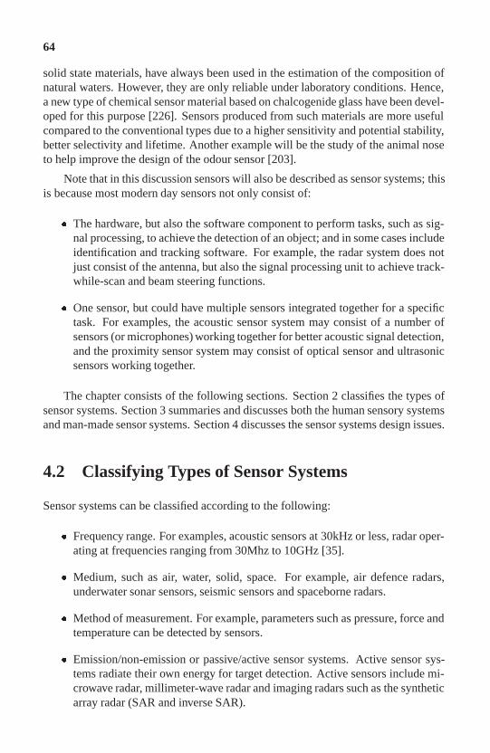
64

solid state materials, have always been used in the estimation of the composition ofnatural waters. However, they are only reliable under laboratory conditions. Hence,a new type of chemical sensor material based on chalcogenide glass have been devel-oped for this purpose [226]. Sensors produced from such materials are more usefulcompared to the conventional types due to a higher sensitivity and potential stability,better selectivity and lifetime. Another example will be the study of the animal noseto help improve the design of the odour sensor [203].

Note that in this discussion sensors will also be described as sensor systems; thisis because most modern day sensors not only consist of:

� The hardware, but also the software component to perform tasks, such as sig-nal processing, to achieve the detection of an object; and in some cases includeidentification and tracking software. For example, the radar system does notjust consist of the antenna, but also the signal processing unit to achieve track-while-scan and beam steering functions.

� One sensor, but could have multiple sensors integrated together for a specifictask. For examples, the acoustic sensor system may consist of a number ofsensors (or microphones) working together for better acoustic signal detection,and the proximity sensor system may consist of optical sensor and ultrasonicsensors working together.

The chapter consists of the following sections. Section 2 classifies the types ofsensor systems. Section 3 summaries and discusses both the human sensory systemsand man-made sensor systems. Section 4 discusses the sensor systems design issues.

4.2 Classifying Types of Sensor Systems

Sensor systems can be classified according to the following:

� Frequency range. For examples, acoustic sensors at 30kHz or less, radar oper-ating at frequencies ranging from 30Mhz to 10GHz [35].

� Medium, such as air, water, solid, space. For example, air defence radars,underwater sonar sensors, seismic sensors and spaceborne radars.

� Method of measurement. For example, parameters such as pressure, force andtemperature can be detected by sensors.

� Emission/non-emission or passive/active sensor systems. Active sensor sys-tems radiate their own energy for target detection. Active sensors include mi-crowave radar, millimeter-wave radar and imaging radars such as the syntheticarray radar (SAR and inverse SAR).

65

Passive sensor systems rely on natural or human-made radiation from thetarget for detection. Passive sensors cover acoustic sensors, thermal sensors(electro-optical systems, such as infrared search and track or forward-lookinginfrared sensors) and electronic support measure (ESM).

� Methods of intelligence information sources. For example, intelligence in-formation sources collected from radios are known as communication intel-ligence (COMINT) and information from human is known as human intelli-gence (HUMINT). The various intelligence1 sources are classified and shownin table 4.1.

Classification Source RemarkHUMINT Human Personal observation and reports.(Human Visual observation by pilots of targets.Intelligence) Human deduction or inferences from

conversation, etc.COMINT Communication sources Internal content of messages.(Communication such as UHF, VHF, HF External characteristics of theIntelligence) radio transmission such as rate and

number of transmission and interactionbetween communication nodes

ELINT Electronic passive Parameters such as pulse width,(Electronic receivers, such as pulse repetitive interval,Intelligence) electronic support frequency and

measure (ESM) system scan intervalIMINT Imagery sources Observation and(Image such as EO (e.g. discrimination of objectsIntelligence) CCD camera and IRST) Example: Two tanks observed

SAR and FOPEN at location XOSINT Internet, newspaper Key feature of interest(Open Source TV, radio, etc. collection of informationIntelligence)

Table 4.1: Classification based on intelligence sources

Note: COMINT and ELINT belong to the category of signal intelligence (SIG-INT) sensors.

4.3 Sensing Technology in Perspective

Table 4.2 shows the human sensory systems which are by nature passive, i.e. theydo not emit signals but receive them. The main sensory systems are: eyes for vision,ears for hearing, tongue for tasting, nose for smelling and the skin for the sense ofpressure and temperature. Of all the sensory systems, the brain processes a largepercentage of the information coming from the eyes.

1Note that the word intelligence in this paragraph refers to information or news collected by organisa-tions or agencies. Such information is normally classified data.

66

Sense Sense organs Physical interaction Sensed resultssensed

Vision eyes light colors(electromagneticwaves) high spectral resolution

Hearing ears sound waves tones

high temporal resolutionTouch,example of receptors pressure pressure, contacttemperature mainly (direct contact, vibration,and in the motion, etc.) temperature -pressure skin hot and cold,receptors thermal flux varying spatial

resolution throughoutthe body - highestin the finger tips

Smell receptors in chemical various scentsthe nasal substancespassages

Taste taste buds on chemical sweet, sour,the tongue substances bitter and salty

Balance semicircular gravity orientation with regardscanals of the to forcesinner ear

General throughout chemical hunger,sensations body balances thirst and control

Table 4.2: Human sensory systems

Table 4.3 shows an example of man-made sensor systems. Note that this list isby no means exhaustive. Man-made sensor systems are both passive and active types.The passive sensor systems are like the ears, the imagery active sensor systems arelike the eyes and the chemical sensor systems are like the nose to the informationprocessing unit of an intelligent system.

In the following subsection, we will briefly describe the man-made sensor sys-tems that are commonly used in civilian and military environments. These are:

� Radar systems;

� Electro-optic systems;

� Acoustic and sonar systems;

� Magnetic sensor systems;

� Chemical sensors;

� Microsensors.

67

Sense Sensor systems Physical Sensed results Applications Remarksinteraction

Vision Radar systems: image, range, air-defence� Imagery radar (SAR, range rate radar, airand FOPEN). electro- and bearing traffic active� MTI radar. magnetic range, control,� Laser radar. waves range rate airborne and� Doppler radar. and ground� MMW radar. bearing tracking radarElectro-opticalsensor systems: light waves images passive� Quantum detector video camera� Thermal detector Infrared scanner

Hearing Acoustic and sound waves range and detect air, passive/sonar sensor bearing surface and activesystems subsurface

objectsTouch Seismic, pressure, range and nuclear passive

temperature and temperature bearing detonation,pressure sensor and vibration object movementsystems on ground

Smell Chemical and chemical detection of passivebiological sensor substances gas compounds,systems and elements and

biological agents virusesOther Magnetic sensor magnetic signal target location altitude control passivesensory systems of staellitessystems Shear and stress fluid shear/stress fluid dynamic passive

sensor systems sensitivity monitoring

Table 4.3: Man-made sensor systems

68

4.3.1 Radar systems

The radar system is one of the most popular sensor used in military and civilian ap-plications. It was introduced in World War Two and since then the technology hasgrown and expanded rapidly. Radar is used in air (all commercial and military air-crafts are normally installed with a radar), on land (ground radar or radar on groundvehicles for air surveillance or detecting ground targets) and at sea (both surface(e.g. ship) and submerged (e.g. submarine)). Radar can detect both static and mov-ing targets. The probability of detection of a target is often a function of the radarcross section (RCS) of the target and the signal-to-noise ratio due to the backgroundnoise. There are many different types of radar systems. The following subsectionswill briefly describe some of these radar systems.

4.3.1.1 Imagery radar

There are two broad categories of imaging radar namely: the real array and syntheticarray. Both the real and synthetic arrays obtain the x-direction (or range resolu-tion) by controlling the transmitted pulsewidth. The real array radars obtain they-direction (or azimuth resolution) from the antenna beamwidth. Since the antennabeamwidth is inversely proportional to antenna length, the y-direction of the realarray radars could be improved by using long antennas (narrow beamwidth).

Synthetic aperture

The synthetic array radar is also known as the synthetic aperture radar (SAR). Thedevelopment of the SAR was motivated by the desire to use smaller airborne anten-nas while increasing the y-direction resolution for ground mapping. SAR use theincremental Doppler shift between adjacent points on the ground, rather than the an-tenna beamwidth, for the y-direction resolution. The SAR radar provides both fineand coarse resolution imagery in spot and strip modes.

Foliage penetrating (FOPEN)

The foliage penetrating radar operates on the principle that different radar frequen-cies passes through foliage with different degrees of easiness. The longer wave-lengths in the UHF section of the microwave spectrum penetrate the foliage moreeasily than the shorter wavelengths, or conversely are reflected less. It is thus possi-ble to create a true ground surface DEM, hence permitting the mapping of the earth’ssurface which is covered under a forest canopy.

69

4.3.1.2 Moving target indicator (MTI) radar

MTI radar is used to detect moving targets. Moving target’s echo pips (or returns)have a phase shift caused by the motion of the target. This echo pips can be obscuredby the other fixed target echoes. Hence, the moving target indicator (MTI) circuitryin a radar system can eliminate the fixed target clutter, and show the moving objects.The returns also enable the computation of the target speed and the target orientation.

4.3.1.3 Doppler radar

Doppler radars can be categorized as:

� Continuous wave (CW) Doppler radar.

� Pulse Doppler radar.

The Doppler radar typically operates at less than 15 GHz. The CW Doppler radartransmits a constant frequency signal that detects relative motion between targets,clutter and the radar through the Doppler principle. It is capable of detecting tar-gets that are masked by ground clutter, and are relatively easy to build and requireminimal transmitted signal bandwidth. The target range-rate is measured using spe-cialized techniques, e.g frequency modulation of the carrier frequency or multiplepulse repetition frequencies. However, a disadvantage of the Doppler radar lies inthe frequency stability of the transmitted signal and the subsequent signal-processingmechanization to maintain the frequency shift achieved between the transmit and re-ceive frequencies.

4.3.1.4 Millimeter-wave (MMW) radar

The MMW radar has a wide bandwidth which is necessary for fine range resolutionused in target imaging or reduction of clutter. For the detection of targets withinshort range (10Km), tactical MMW are produced. Such MMW radars are able todetect stationary targets. MMW radars are produced at higher frequencies, from 35to 230 GHz, due to the low atmospheric attenuation at such frequencies. As such,the angular position resolution of targets can be increased.

4.3.1.5 Laser radar

Laser radars2 use narrow beamwidths. Laser radars are not suitable for searchingcapability. However, they are able to detect range fairly accurately and are oftenused in conjunction with passive infrared search and tracking (IRST) systems andthermal imaging systems. In these applications IRST or thermal imagers locate the

2Laser radar is also categorized under the electro-optical sensor system.

70

potential targets in large volume and the laser radar system is pointed in the directionof the target to obtain the range. The laser radar could also be used to confirm theexistence of a target.

4.3.2 Electro-optic systems

Electro-optic systems typically interact with optical fields. They provide still imagesand videos. Most of the electro-optic systems are passive devices. These systemsnormally consist of the fonts (mirrors, lenses, filters), detectors, scanning circuitry,signal processing and display. Electro-optical systems can be classified into twotypes, namely, the quantum detector and thermal detector [189].

4.3.2.1 Quantum detector

Quantum detectors use semiconducting materials to collect the energy of photons.As the electrical properties of the semiconductor are changed by the absorbed pho-tons, an optical signal is detected. Products, such as digital camera, video camera,which use CCD array as image sensors, belong to this type.

4.3.2.2 Thermal detector

Thermal detectors absorb photons over a relatively broad band of optical wave-lengths. This absorbed energy causes a rise in the temperature of the detector mate-rial. The optical signal is detected by the change in temperature.

Infrared Search-Track sensors - IRST

Infrared (IR) sensors are passive sensors which depend on emitted energy, such assunlight, to distinguish targets from the background, by the IR radiation they emit.IRST sensors operate by scanning a single or an array of detectors over a surveillencevolume for infrared point sources intersected by the targets. Target tracks are thenformed as the detections are measured. IR sensors that are mounted on aircraft fordetecting ground targets are also know as forward looking infrared (FLIR).

4.3.3 Acoustic and sonar sensor systems

Acoustic sensors detect, track and classify targets using acoustic signals which arepropagated through water, solids or the air. Examples of such sensors are: sonarsensors for ships and submarines, microphonic sensors for aircraft and vehicles onthe ground, and seismometers for nuclear detonation and movement of troops. Inparticular, the sonar system consists of various stages: detection of the planar wave-front from a point source using an hydrophones array, beam forming to provide an

71

integrated signal for further processing, null steering for the forming of multipletarget-observing beams to track and search for targets, noise cancellation of additivenoise, and removal of noise and detection of targets through spectral analysis.

4.3.4 Magnetic sensor systems

The application of such sensors is very wide and can be classified into two levels.The first level is the direct determination of the magnetic field itself. The second levelis the indirect method. Each one of these applications can be used as a componentin a system or equipment, such as a process controller in a submarine or satellitenavigation system.

4.3.4.1 Direct measurement of the magnetic field

The purpose of direct measurements is to gather information about the direction andmagnitude of the magnetic vector itself. It includes:

1. Altitude control of satellites, submarines, balloons and aircrafts;

2. Geophysical and geological investigations;

3. Classical and electronic compasses;

4. Prediction of volcanic eruptions and earthquakes;

5. Retrieval of data stored on magnetic tapes or disks;

6. Acceleration systems used in nuclear physics.

4.3.4.2 Indirect measurement

The indirect measurement is further classified into two areas. The first area is in themeasurement of electrical quantities, such as current and power. The second area isthe recording of non-electrical and non-magnetic quantities, whereby the informa-tion is magnetically encoded and the output sensor signal becomes the carrier of theoriginal quantities, such as linear and angular position, stress, force and weight. Theapplication of indirect measurements includes:

1. Contactless keys and DC motors, remote-control values and door locks;

2. Transducers for linear detection, such as proximity keys and position sensors;

3. Traffic detection, such as determination of submarine location and determina-tion of the spatial positions of ferromagnetic objects.

72

4.3.5 Chemical sensors

Chemical sensors are for detection of gas, odor, concentration, pH and ions. Theyare devices that convert a chemical state into an electrical signal. A chemical state isdetermined by the different concentrations of elements such as atoms or moleculesto be detected. Thus, a chemical sensor gives a signal that in some way is related tothe chemical state it is exposed to.

The NASA Lewis Chemical Species Gas Sensors Team are developing hydro-gen, hydrocarbon and nitrogen oxide sensors for aeronautics and aerospace appli-cations [225]. For example, a hydrogen sensor is used to detect the presence ofhydrogen. Presence of hydrogen may potentially indicate that the environments areexplosive or dangerous.

4.3.5.1 Gas sensors

A gas sensor is a chemical sensor operated in the gas phase. The response, x, from agas sensor to a single gas can be described as:

x = fgas(Cgas) (4.1)

where fgas is a (usually non-linear) function and Cgas is the concentration of thegas. The response is in most cases the difference or ratio between the steady-statevalue when the sensor is exposed to the test gas and the value from the sensor, suchas derivatives or integrals over certain time intervals. Two important parameterswhen describing the response from a sensor are the sensitivity and selectivity. Theseparameters are easy to define and interpret for a sensor sensitive mainly to one gas.The sensitivity, Ygas, for the sensor towards this gas is then defined as:

Ygas =@x

@Cgas(4.2)

In general, the sensitivity is a non-linear function of concentration. The selectivity,E, of a single sensor is usually defined as the ratio of the sensitivity related to thegas to be monitored and the maximal sensitivity to all other interfering components.

E =YgasP

allothergases(Y )(4.3)

One main target of chemical sensor research is to enhance the sensitivity and selec-tivity of the sensor for a specific compound.

A gas sensor usually consists of two parts: the sensing material and the trans-ducer. The sensing material interacts with the analyte, e.g. by absorption/desorptionor chemical reactions on the surface and/or in the bulk of the sensor material. Theinteraction changes some physical properties of the sensing material, for instance themass or the electrical conductivity, which can be detected. The transducer converts

73

the chemical information into an electrical signal. A number of possible transducerprinciples can be used in chemical sensors, e.g. changes in conductivity as detectedby voltage drop over a series resistor.

4.3.6 Microsensors

Most chemically related sensors are relatively small. A number of temperature andcorrosion detection sensors are also available in miniature size and could be builton top of silicon chips. An example of micro sensors includes a single photodetec-tor. Photodetectors, sometimes also known as photosensors, are simple sensors thatdetect a single source of energy and produce an output (normally the output is anelectrical signal to indicate the presence of an energy source).

Oak Ridge National Laboratory has developed a micro wireless sensor contain-ing an IR LED for signal transmission of up to 1 km. The sensor is sufficiently lightand small to be carried on top of a bee [149].

4.4 Sensor System Design Issues

While the eye cannot hear, so is the ear that cannot see. Every designer of sensortechnology would want to achieve a single all-mighty and intelligent sensor system.But it is difficult, if not impossible to achieve. The physical law of nature alwayslimits our design of sensor capabilities.

Sensor system design issues include:

� Power management. Management of power is particularly critical for stan-dalone sensor systems. The ability to design low power consumption technol-ogy and the ability to turn on the sensor only when it is necessary, will helppower management. The quest to design a better standalone power source is acontinuous research area.

� Physical constraint. The size of the sensor system and the material it needs tobe used will be affected by the kind of physical applications.

� Operational environment. Where the sensor systems will be operated will af-fect their physical design. There are always great differences in design speci-fication for a sensor system built for indoor compared with one for outdoor.

� Specification. This affects the resolution, accuracy and coverage of the sensorsystems during design phase.

� Cost constraint. The uses of sensors are frequently affected by cost. Cost willdrive the market on how a sensor will be used.

74

� Integration with other sensors. Integration of sensors will be an increasinglyimportant design issue. This will be further discussed in the next subsection.

4.4.1 Multiple sensor integration

Every sensor system has a specific ability to detect, identify and track specific ob-ject/s in a certain environment. The integration of every sensor or sensor systems,by harnessing and controlling their individual strengths and capabilities, could leadto the development of very powerful and/or intelligent sensor systems. Such an inte-gration process would involve multiple sensor data fusion technology. This will bediscussed in part 2 of this book.

4.4.2 Sensing platforms

Sensors can be placed on different platforms that could be mobile, static and di-versified structures. Here, we will consider sensors located on a single or multipleplatforms.

� Single platform with multiple sensing devices. The major reasons to employmultiple sensors on a single platform are that the various sensors providedifferent, often synergistic, information; search different locations in space;provide redundancy in a target-rich environment and/or under high reliabilityrequirements; and provide increasingly accurate information (e.g., warning,general location, specific location) [43]. A typical example of such system is afighter plane that carries radar systems and infrared search-and-track sensors.

An example of a single platform with multiple sensing devices is the head ofan animal, where the various sensors (eyes, nose, ears) are positioned in sucha way that a movement of the head will effect one of the sensors, but willalso help the other sensors to provide a more comprehensive picture of thesurrounding environment.

� Multiple platforms with multiple sensing devices. In most modern militarysystems, several different platforms are usually involved to aid the data fusionprocess to produce a more conclusive situational picture. This type of systemmay also be thought of as a combination of several single platforms that aresimilar if not the same. Example, the DARPA’s Unmanned Ground Vehicleprogram, see [61], with a unit of autonomous vehicles equipped with cameras.A major problem associated with such multiple platforms, as pointed out in[43], is the transformation of sensor estimates from the coordinate system ofone platform to that of another. If the transformation is sufficiently inaccu-rate, targets common to both sensors cannot be recognized (i.e. associated)and false targets are generated. Hence accurate coordinate transformation isimportant. This is part of the data fusion process. The data and informationfusion will be discussed in Chapter 5.

Part II

CHAPTER 5

Fusion Systems for IntelligentProcessing

Data fusion is deceptively simple in concept but enormously complex inimplementation.

US Department of Defense, 1990.

5.1 Data and Information Fusion System - What andWhy

Fusion involves the combination of data and information from more than one source.Data and information fusion is becoming an important field of study due to an in-crease in data and information flow, and the continuous improvement in communi-cation, computing and sensor technology. This increase is shown in the followingareas:

� research and publication of data fusion work.

� military and civilian interest in integrated/networked systems that need dataand information fusion, such as network centric warfare and e-commerce.

Fusion systems are applied to the medical field, earth resources monitoring, weatherforecasting, vehicular traffic control, robotic navigation, financial analysis, and mili-tary command and control (C2) systems. The sources of data could be from sensorsor textual1 reports. Textual data are sometime known as information, whereas thesensor observations are data. Hence, the term sensor fusion or information fusion isused interchangeably, depending on the data sources. In this book, the general term

1Textual refers to data with assigned attributes that is represented in text form.

80

data and information fusion are used. Figure 5.1 illustrates the difference betweendata, information and knowledge. Knowledge is the ability to use information. Itinvolves understanding the information and is derived from the information process.Knowledge is situation dependent and requires intelligent process of information.Information and knowledge are an integral part of cognition 2. The ability to fusedata and information for meaningful use as a form of knowledge in machine is anessential fusion process.

Logic

and intelligence

Storage and organizationof information

Dynamicsituation

Assigned attributeswith limited logical

Intelligent process

relationship between data

Limited prefined attributes

update

Knowledge

Logic

Data

Information

Figure 5.1: Data, information and knowledge.

Why data and information fusion systems? Fused data/information are muchmore enriched in information than data from a single source, else the data/informationwould not be fused. Hence, fusing data from multiple sources is an intelligent pro-cess. This intelligent fusion process is well illustrated in how our brain fuses datafrom our body’s sensory systems such as eye, ear, nose, tongue and skin. Our body’ssensory systems provide sense data from our environment via the nervous system tothe brain. The brain fuses this information to achieve the awareness of our surround-ing environment and attempts to derive knowledge, draw conclusions or inferencesfrom the fused information. Figure 5.2 shows an analog view of an intelligent fusionsystem as that of a brain using multiple sensory information sources.

Other reasons on why we need data and information fusion systems are:

� Robust System. A system that depends on a single source of input is not robustin the sense that if the single source fails to function properly, the whole systemin operation will be affected. However, the system fusing several data sourcesis more robust while in operation or has a higher fault-tolerance rate since

2Cognition is defined as the process of knowing, perceiving and conceiving. Cognition involves theintellect and the mental process in obtaining and processing of knowledge and information.

81

Figure 5.2: Intelligent fusion process.

other sensors in working order are able to provide similar, if not better data forprocessing.

� Better situation awareness and inference, hence faster reaction time. By takingadvantage of different sources or sensors’ accuracy, the combined and fusedresults would give a better picture of the situation and hence improve infer-ence, which in turn, would lead to better decision making. This is particularlytrue in military scenarios where increases in the accuracy of weapons and tar-gets mobility require quicker responsive detection and countermeasure reac-tions. More sensors are able to provide additional information on the targetand hence better tracking and faster reaction time for countermeasures.

� Improve data accuracy and reduce data uncertainty and ambiguity. Multipleindependent sources of data collectors can help improve data accuracy andreduce uncertainty after intelligently fusing and removing the ambiguity ofthe data.

� Extended coverage. More data sources will provide extended coverage of in-formation on an observed object or event. Extended coverage can be applied

82

to both spatial and temporal environments.

� Cost effectiveness. With the reduced cost of computing, communication andnetwork resources, it is, in general, more cost effective to depend on multi-ple sources of data input, than relying on a single source to provide all thenecessary information. For example, to build a single sensor that can performmultiple functions is much more expensive than to integrate several simple andcheap sensors with specific functions. This is also related to the next point onno single perfect source.

� No single perfect source. Most sources of data collector, such as sensors, areonly useful in certain environments. Information gathered by a single sourcecan be very limited and may not be fully reliable and complete. For examples,contact sensors can only detect an object on contact, acoustic sensors can onlydetect objects that emit acoustic signals, vision sensors are critically dependenton the ambient lighting conditions and electronic surveillance sensor can onlydetect objects that emit electro-magnetic waves. Hence, it is difficult for onesource to meet all the needs.

This chapter is arranged as follows: Section 2 will discuss the multiple levelsof data and information fusion process. Section 3 will present the issues in fusingdata. Section 4 will discuss the cognitive intelligence for intelligent fusion systems.Section 5 will present the fusion system architecture. Section 6 will briefly discussthe possible techniques and algorithms for fusing data and information. Section 7will discuss the complementary and competitive data. We conclude with section 8.

5.2 What are the Different Levels of Fusion Process?

The Joint Directors of Laboratories (JDL) Data Fusion Subpanel of the US Depart-ment of Defense (DOD), defined data fusion as a multilevel, multifaceted processdealing with the association, correlation, estimation, and combination of data andinformation from multiple sources to achieve refined entity position and identity es-timates, and complete and timely assessments of resulting situations and threats andtheir significance [121]. This section expands on this definition. The multilevel datafusion process could be broadly divided into 5 levels. We categorized these 5 lev-els into the two stages of processes, namely low-level fusion process and high-levelfusion process, as shown in Figure 5.3.

� Low-level fusion process.

– Level 0 - Source pre-processing. This is the lowest level of the data fu-sion process. The kinds of fusion work include signal processing fusion(fusion at signal level after a signal conditioning process) and imageryfusion at pixel level (also known as pixel level fusion). Hence, most of

83

Fusion Process

Low−level Fusion Processes

High−level Fusion Processes

Level 2 (Situation Assessment)

Level 3 (Impact Assessment)

Level 4 (Refinement Process)

Level 0 (Sources Pre−Processing)

Level 1 (Object Assessment)

Man−in−the−loop) (Automatic and/or with

Figure 5.3: 5 levels fusion process.

these sources involve individual sensor’s multiple detection inputs to thesignal-processing engine. If the sources are textual, such as from pressor Internet, this stage also includes information extraction. This level offusion also looks at reducing the quantity of data and retaining usefulinformation for the higher-level fusion processes.

– Level 1 - Object assessment. This level of fusion uses the processed dataobtained at level 0. The common processing needed at this stage are dataand time alignment, association and correlation, grouping or clusteringtechniques, state estimation and state vector fusion, deghosting of falsetarget (for passive sensors), identity fusion and combining of feature ex-tracted from images (also known as feature-level fusion). The end resultsof this fusion process are object discrimination (object classification andidentification) and object tracking (object state and orientation).

� High-level fusion process. High-level fusion normally starts at the point wherethe objects are known i.e. the type, location and movement (orientation andhistory points), and quantity of these objects. Decision-level fusion, com-

84

monly discussed in the fusion community, could be said as belonging to thehigh-level fusion process. In most cases, fusion at levels 2, 3, 4 will ultimatelycontribute to decision making.

– Level 2 - Situation assessment. Level 2 processing seeks for a higherlevel of inference above level 1 processing. According to the JDL (US,DOD), situation assessment identifies the probable situation using theobserved data and events. Basically, it establishes a relationship amongobjects. Relationships (such as proximity, temporal and communica-tion from content and non-content sources) are assessed to determinethe meaning of entities or objects in a specific environment (such as ter-rain, surrounding media, weather, vegetation and area of interest). Thegoal at this level includes: deriving higher-order inference and identify-ing meaningful events and activities (or pattern, in general). An exampleof higher-order inference for classification of organization structure isthe clustering of platoons to infer a company. And examples of activitiesare coastal surveillance operations, military training exercises, defensiveoperation and illegal animal hunting. An example of an event is an air-craft crossing the border between two countries. Hence the output ofsituation assessment is a collection of higher-order inferences in chrono-logical order, which provides a view of what is happening in the world.

– Level 3 - Impact assessment. This level is classified as impact assess-ment. Note that the revised JDL model (1998) has also used impactassessment in place of the threat assessment. As the name implies, thislevel is to assess the impact of the activities and events derived at level 2to own perspectives or in military strategic planning perspectives. Thisincludes:

� Assessing the level of threat or danger. For example:

� The activity of coastal surveillance operations - is this a highthreat due to our important assets near the surveillance area, or

� Assessing the capabilities of the adversary’s forces with respectto own forces’ strength. What are the adversary’s defensive andoffensive capabilities?

� Predicting the possible outcome. For example, predicting the possi-ble adversary’s intentions and predicting the impact of illegal animalhunting on the region’s ecology. If unable to predict the intentions,what are the different possibilities?

� Assessing the vulnerabilities of our assets. What are the risks to ownassets and forces?

� Possible own forces’ cause of actions. What are the actions to taketo ensure own survivability or minimise the risk?

– Level 4 - Refinement of fusion process. The last fusion process is therefinement process. The refinement process is to improve the data fusion

85

from level 0 to level 3. This level is performing resource management,in particular, of the sensor resources (as the sensor is the main focus,this level is also known as sensor management). The common aim is toachieve an effective resource management by performing: task priority,cueing, scheduling, allocation and control of resources. These will formpart of the sensor management process that serves as a feedback loop forthe complete sensor fusion process.

Figure 5.4 shows the idealized flow of the 5 levels data fusion process.

Resources

(e.g. resource

selection,

detection

threshold,

Controllable

Detection

Signals / FeaturesSignal

modes,etc)

Level 0Source Preprocessing

Resources

Level 2Situation Assessment

Level 1

Impact Assessment

Situations/ Plans

Level 3

Object Assessment

Level 4

Process

Refinement

(Resourse

Management)

Measurements

Activities

&Events

Information

Object

(Processed data)

Figure 5.4: Possible logical flow of the 5 levels fusion process.

86

5.2.1 Fusion complexity

The complete JDL data fusion model encompassed the complex integral of multiplesensory systems and the interpretation of the complete chain of data and informationfor situation and impact awareness. At the low-level fusion process, it is an immedi-ate or short-term demand for situation awareness. At the high-level fusion process,it is toward the projection or long-term demand for situation and impact awareness.The refinement process will then assist to manage the multiple sensory systems (orsources) to meet the short-term and long-term demand.

The complete fusion process is a complex task. The low-level fusion will needto address the complexity of association, short-term history process and structuralissues. While high-level fusion needs to handle the intelligent integration of currentinformation with long-term memory information and information recall issues.

In military perspective, how close are data and information fusion processes infulfilling the principle found in Sun Tzu’s Art of War [235], is for one to find out. Apartial quote from Sun Tzu’s works regarding this principle is as follows:

He who has a thorough knowledge of himself and the enemy is bound to win in all battles. Hewho knows himself but not the enemy has only an even chance of winning. He who knows not

himself and the enemy is bound to perish in all battles.

Know your enemy, know yourself, and your victory will not be threatened. Know the terrain,know the weather, and your victory will be complete. [235]

5.3 Issues on Fusing Multiple Sources

Data and information fusion are a multi-disciplinary subject. Data could come fromdiverse sources where information of the data could be ambiguous, noisy and thequantity could be substantial. Hence, it is not a trivial matter to solve data andinformation fusion problems.

Listed below are some of the common issues one will face in fusing multiplesources of data:

� Data dimensionality and alignment. Different sensors have different measure-ment data and hence different dimensionalities and features. Data alignmentand transformation would be needed to achieve common format and standards.Note that the registration process is considered as part of data alignment. Forexample, different sensor systems may have different:

– Coordinate systems such as Cartesian, spherical and polar coordinates,latitude-longitude-altitude (or LGZ), North-East-Down (or North-East-Up) and Military Grid Reference System (MGRS) representation.

– Measurement units such as mile, meter, feet and inch.

87

– Size of data (object state observable) such as different dimensional space.

– Features such as frequency, amplitude, imagery and non imagery.

– Data resolution and accuracy.

– Common reference. Sensors in same or different platforms need to bealigned into a common spatial reference.

Hence techniques are required to perform data transformation and normaliza-tion to a common format and standard that are appropriate for data fusionprocesses.

Data alignment is required to transform observed data from many differentsources to a common format. Data alignment is part of the registration process.

� Data incest and reliability. Distributed and decentralized data fusion need tohandle the problem of data incest and reliability issues. Figure 5.5 illustratesthe problem of data incest. Ideally each fused data should contain informationon whom is contributing it (this is related to indicating the data dependencyand independency factors) and its source’s reliability. However, tagging suchinformation across many nodes is a complicated task and may not be easy toimplement in practice.

� Time alignments. The synchronization of the data time is important. Thisis because only data that are ‘close’ in time can be integrated, if meaningfulresults are desired. This is particularly important for competitive data. Thecloseness of time or the window period where the data can be fused dependson the types of fusion system. Time-critical fusion systems such as fusionsystem on-board air platform, the time window is typically in micro or minisecond; whereas fusion systems for non-real time analysis that depend on re-port sources that may take minutes or hours to arrive, the time window ofcloseness could be in the order of minutes or hours.

However, for complementary data, the closeness of time may be relaxed. Thisis because complementary data may still provide useful information to thefusion system even if the data sources are not sufficiently close in time. Formore discussion on competitive and complementary data, please see section5.6.

Time alignments are complicated by:

– Sensors located at geographically different areas and at different plat-forms.

– Time difference of arrival due to different signal propagation speeds e.g.acoustic signal vs electromagnetic signal vs seismic signal.

– Data source update rate.

– Sampling rate. Sampling rate of the sensor measurement data for mostintegration algorithms need to be the same.

88

Node 2Node 1

Node 1

Node 2 Node 3

Node 3

No target detected but if Node 1detects a target, then thereprobably is a target.

Probably a targetover there.

detects a target, then thereprobably is a target.

No target detected but if Node 2

Probably a targetover there.

Node 3 detects a target

Target detected (50% confidence)

must be a target. (90% confidence)as well. Therefore, there

Figure 5.5: Example of data incest. Node 1 communicates its detection tonode 2. Node 2 passes the message to node 3. Node 3 broadcaststhe message and node 1 receives. Node 1 assumes that node 3has the same detection and hence increases its confidence of thedetected target.

Time stamping and a common clock for synchronization will have to be es-tablished. Techniques are required to resolve the time delay due to signalpropagation and sensor detection. Alignment to ensure common time framemay be needed.

� Sensor operation platforms.

– Single or multiple platforms. Sensors in a single or multiple platformhave their own unique time synchronization problems.

– Static or moving platforms. Sensors are in moving or stationary plat-forms. It is certainly not a trivial problem when the sensors are in differ-ent moving platforms e.g. it may not be feasible to achieve any meaning-ful results having acoustic sensor on a continuous fast moving platform.

89

Speed of the moving platform is a factor that needs to be considered.

� Quantities of sensors used. The increase in the number of sensors availablemay result in an exponential increase of:

– Fusion engine design complexity.

– Data storage structural complexity.

– Communication costs [109].

It is common belief that with more sensors, hence more data, is never theoreti-cally bad for decision making. However, as pointed out by Treece [221], moredata or information is damaging to the final answer under certain conditions.Some of these conditions are related to data reliability and the environmentthe sources are operating on. More studies and investigations are needed toidentify the conditions that could be damaging for adding more data.

� Sensor selection strategies. Luo and Kay [146] pointed out that the sensorselection is one of the integration functions that can enable a multi-sensorsystem to select the most appropriate configuration of sensors from amongthe sensors available. Therefore, proper sensor selection strategies need to bestudied. Factors affecting the sensor selection include:

– Target dynamics.

– Target densities (e.g. closely-spaced targets).

– Background noise sources (e.g. high clutter background due to multipathreflection).

– Sensor performance (e.g. probability of detection).

� Concepts of operation. The high-level fusion process would need to takeinto consideration the concepts of operation, particularly in a military con-text. With increasing complexity of the battlefield, meaningful integration andfusion can only be established if the operational doctrine is well understoodand the goals are clear.

� Organizational structure and workflow. In order to provide meaningful fu-sion results, some understanding of the organizational structure and workflowwould be useful. Different groups of people in the organization look for dif-ferent information, hence fusion system would need to fuse the correct set ofdata and information that the people are looking for.

� Physical and operational constraints. The choice of fusion architecture andtechniques are sometime affected by the physical and operational constraints.

The solutions to the above issues are non-trivial. The degrees of difficulty alsodepend on the level of the fusion process and fusion architecture used. To derive

90

higher intelligence inference, such as the human brain intelligence, the cognitiveintelligence process will need to be studied. The next section will cover a brief de-scription of the cognitive intelligence. And since the fusion architecture will alsoaffect the fusion system design (system engineering design perspective) and the fu-sion algorithms (in term of efficiency and effectiveness), the section after cognitiveintelligence will discuss the fusion architecture.

5.4 Cognitive Intelligence

The fusion issue at high level involves understanding of information to perceive andconceive for situation and impact assessment and ultimately awareness. Today, thereis no known machine that could do that as well as the human brain can. Hence to en-gineer this fusion process, the understanding of how our brain processes informationand knowledge will be important - specifically the aspect of intelligence pertainingto cognitive processes, i.e. perception, learning, information retrieval from memoryand inference, more commonly known as cognitive intelligence. The study of cog-nitive intelligence includes: understanding the complex human brain in coping withlife situations, such as its ability to adapt to new conditions, learn new things, recallinformation and apply knowledge to solve problems.

5.4.1 How to make sense of information?

What is the cognitive process that enables one to decide which pieces of informationare more relevant than others? And how to obtain meaning from data that is other-wise difficult to draw any useful conclusions from? How to recall information at theright time for a useful process? How to understand what others think?

The attempt to engineer the cognitive process has led to cognitive psychology 3,knowledge engineering, ontological engineering, memory engineering, computa-tional intelligence (e.g. biologically-inspired algorithms), human factor study andmany more. More recently, the term cognitive informatics was coined for the studyof natural intelligence. Cognitive informatics study the internal information pro-cessing mechanisms and natural intelligence of the brain [229] and has originatedfrom information theory and contemporary informatics 4. Cognitive informatics lookinto how human beings acquire, process, interpret, and express information by us-ing the brain and how we understand the mind of different individuals. This newinterest has led to the First IEEE International Conference on Cognitive Infomatics(ICCI’02) held in 2002.

3Cognitive psychology includes studies of perception, memory concept formation and problem solv-ing.

4Informatics refers to the science of information. It involves the studies of the nature of information,it’s processes, and ways of transformation between information, matter and energy.

91

The other aspect of the cognitive process is in attempting to make sense of infor-mation or also known as sensemaking. In the general sense, the word ‘sensemaking’refers to the derivation of an understanding of a problem given a large set of datathat is complex and sometimes even self-conflicting. Sensemaking is a complicatedprocess and is described as a cognitive task model [53, 184]. As such, it is subjectiveand is dependent on many factors, such as the point-of-view of the people performingit and diversity of the group. Sensemaking is used in situations where informationis often vague and ambiguous. For more information on sensemaking, reader mayrefer to the publication by Leedom [136, 137].

The transformation from information to knowledge is situation dependent [54]and involves smart algorithms. Figure 5.6 shows a possible engineering flow of anattempt to model cognition and high-level fusion to achieve situation and impactawareness.

(Information presentation)Display

Retrievalstrategy

Intelligent process

(Situation & Impact)Awareness state

Decision making

Long-term memory

Short-term memory

InformationData

High-level fusion process

Data/Informationcollection

Sensemaking

Interface design

Knowledge derivation with organized information

Low-level fusion process

(Action)

Other influence factors

Sensory systems

managementResource

stateawareness

ofupdate

Continuous

Human awareness state

Work flow

Organization structure

Culture

Figure 5.6: Possible engineering flow of cognitive and high-level fusion pro-cess.

92

The awareness state is continuously updated within the closed-loop process ofmemory and the intelligent algorithms. The memory engineering process will needto handle the storage and organization of useful information and with the ability torecall or retrieve information to enhance the awareness state. Memory engineeringprocess and intelligent process work hand-in-hand to derive knowledge and updatethe awareness state. The awareness state will continue to evolve from a perceivestate to a comprehension state and finally to a projection state (see Figure 5.7). Theawareness state will be updated with more data and information input.

Perceive state Comprehensionstate

Projectionstate

Awareness stateData & information

Figure 5.7: Possible evolving process of the awareness state.

The intelligent process will involve decision support tools such as the biologi-cally inspired algorithms (or the descriptive techniques), information-theoretic ap-proach, statistical and probabilistic techniques, mathematical modelling and cogni-tive informatics approaches. The iteration between the intelligent process, awarenessstate, memory engineering process and the resource management form the high-levelfusion process.

Sensemaking will encompass the awareness state, the interface design and un-derstanding of the way human make decision. The interface design include howinformation can be best presented so that a human can interpret it correctly and com-fortably. Hence, the interface design will consider human factors such as stress,workload, expectation, cognition, expertise, personality and culture.

5.4.2 Memory structure for cognitive intelligence processing

Memory is an important component in the study of cognitive intelligence. Memory isthe foundation for maintaining a stable state of an animate system. It is also the foun-dation of any natural intelligence [230]. The cognitive memory map plays a role inunderstanding how the brain processes information.The human brain typically can bemapped into the following 4 memory types namely; the sensory memory, short-termmemory, long-term memory and action buffer memory [230]. Figure 5.8 shows thememory structure. Cognitive engineering views the learning as a process in whichinformation is obtained, stored in the long-term memory and able to successfullyrecall it when needed [94].

93

SensoryBufferMemory

Long−TermMemory

Short−TermMemory

ActionBufferMemory

Action

Figure 5.8: The memory structure.

5.5 Fusion System Architecture

There are several ways of classifying data and information fusion system architec-ture. From literature survey and studies, we could classify them into the following 4types of fusion architecture, namely:

� Centralized fusion architecture.

� Decentralized fusion architecture.

� Distributed fusion architecture.

� Hierarchical and hybrid fusion architecture.

5.5.1 Centralized fusion architecture

In a centralized fusion architecture, the fusion unit is located at a central processorthat collects all information from the different sources (Figure 5.9). All decisions aremade at the central processor.

94

Legend:

:measurementsinput - sensor

Central Processor

TrackingFiltering

Processes: Asociation

Figure 5.9: Centralized architecture with a central processor.

5.5.2 Decentralized fusion architecture

A decentralized fusion architecture consists of a network of nodes, where each nodehas its own processing facility. There is no need for a central fusion or central com-munication facility, as a common place does not exist where fusion or global deci-sions are made as fusion occurs at each node, on the basis of local information andinformation from neighbouring nodes [74].

Three characteristics of a decentralized fusion architecture are:

1. No single central fusion centre.

2. No common communication facility.

3. Nodes have no global knowledge of the network topology.

Decentralized fusion architecture could be further categorized as fully connecteddecentralized fusion architecture or partially connected decentralized fusion archi-tecture. Figure 5.10 shows a fully connected decentralized fusion architecture.

5.5.3 Distributed fusion architecture

Distributed fusion architecture is shown in Figure 5.11. Distributed fusion architec-ture is where each sensor’s measurements are processed independently (e.g. performdata association and state estimation) before sending the object (e.g tracks) to a cen-tral processor for further fusion with other distributed sources input. Distributedfusion architecture could be viewed as an extension of the centralized fusion archi-tecture.

5.5.4 Hierarchical fusion and hybrid fusion architecture

The other possible architectures in the literature are a combination of centralized,distributed and decentralized architectures. Here, we classify two types of mixed

95

input - sensor measurements:

where association, filtering and fusion occurs

:

Legend:

Figure 5.10: Decentralized fusion architecture.

architectures, namely hierarchical fusion architecture (see Figure 5.12) and hybridfusion architecture (see Figure 5.13).

5.5.5 Is there a difference between decentralized and distributedfusion?

Although the terms decentralized and distributed fusions are used interchangeably inmost of the literature, there is a slight difference between the two terms.

In a decentralized case, the various decision makers (or estimators or controllers)do not all share the same information at a given time and there are no central facil-ities. In a distributed case, there still exists the notion of central processing. Dis-tributed networks reduce computation and communication by dispersing the workamong a number of hierarchical processors which ‘report’ to a central processor[23].

The difference between decentralized and distributed fusion architecture is shownin Figures 5.10 and 5.11 respectively. However, one common similarity is that boththe distributed and decentralized fusion are able to work in a multiple sensors envi-ronment.

96

CentralProcessor

State VectorFusion

: input - sensor measurements

: single sensor tracking

Legend:

Figure 5.11: Distributed fusion architecture.

5.5.6 Is there a single best architecture?

The answer to the above question is an obvious NO. This is because architectureselection is a function of need, demand, existing connection, data exploitation level,data availability, strategic planning scheme, and the organisational structure usingthe fusion system.

However, centralized architecture is, in general, better discussed, implementedand used than decentralized architecture. Most of the existing fusion systems, in oneway or another adopt centralized architecture. Decentralized architecture is difficultto implement partly due to communication and computing constraints, cost, spatialand temporal issues. Robust decentralized algorithms that could solve these issuesare currently being investigated. For example, using an information filter (IF), ratherthan decentralized Kalman filter (KF), in a decentralized architecture’s state estima-tion process. This is because the information filter is computationally less complexand claims to occupy less bandwidth than the Kalman filter. This will help reducethe computational load and communication costs.

As systems become more interconnected, mixed architectures will prove increas-ingly more popular. For example, building a fusion system where the current sensorsystems have already performed fusion at level 1 process.

Most of the stand-alone platforms (e.g. car, aircraft, ship, tank and single liftsystems) will remain working in a centralized architecture. We refer to a stand-aloneplatform as a system with only one central processor. Transforming multiple stand-alone platforms to decentralized fusion architecture will depend very much on howthe constraints (as stated earlier) could be resolved.

97

LocalFusion Centre

LocalFusion Centre

Legend:

: Input - SensorMeasurements

LocalFusion Centre

Centre

Global

Data Fusion

Figure 5.12: Hierarchical architecture.

5.6 Techniques for Data and Information Fusion

Data and Information fusion techniques are drawn from many disciplines. Figure5.14 shows that the building of data and information fusion systems often involvesmulti-discipline subjects and techniques. These multiple techniques are often appliedjointly or sequentially [92].

5.6.1 Level 1 - Object assessment

At the level 1 fusion process (object assessment), the analysis is more at individualobject. Each object is studied and characterized with regard to its class, position andorientation. The techniques required include data association, state estimation andclassification.

5.6.1.1 Data association and correlation

Data association is the problem of attempting to determine the set of data that re-ferred to the same entity (where entity could be the desired object or event). Is therea difference between association and correlation? Hall [92] defined data associationand correlation as follows:

� Association - The process of assigning and computing weight that relate obser-vations or tracks from one set of data to observations or tracks to another setof data. For example, frame to frame association, observation to observationassociation, observation to track association, and track to track association.

98

Processor

association, filtering and fusion occurs

Processor - where

Processor

:

Processor

Legend:

: Single Sensor Tracking

: Input - sensor measurements

Processor

Processor

Figure 5.13: Hybrid architecture.

� Correlation - The structural, functional or qualitative correspondence betweencomparable entities; a decision making process which employs an associationmetric as a basis for allocating or assigning sensor measurement and/or reportto the hypothesis entities of interest.

Another definition of the term correlation is: Correlation is a bivariate mea-sure of association (strength) of the relationship between two variables.

In simple terms, association involves an action of finding the joint relationship amonga set of data. The findings of this relationship could be used for clustering purposesor identifying data or information that are referring to the same object or subjectmatter. On the other hand, correlation involves understanding the shared relation-ship, or connection of cause and effect between two data or two set of data. Hence,correlation is naturally part of the association process.

99

Signal

Theory

BiologicalScience

Processing

Statistics & Probability

Engineering

PsychologyComputing

Engineering

Data and Information

Fusion System

Science

TheoryControl

Information

Software

IntelligenceComputational

Cognitive

Figure 5.14: Data and information fusion system - multi-disciplinary sub-ject.

Figure 5.15 shows the possible algorithms for performing data association. InChapter 6, we will further discuss the issues and some of the techniques used fordata association.

5.6.1.2 State estimation

State estimation is the problem of attempting to determine the value of an object’sstate, given the observations or measurements of the object (commonly the termsystem is used rather than object for state estimation). Figure 5.16 shows the variousfilters that could be used for state estimation. It is noted that for state estimation, theIMM (Interactive multiple models) algorithm is well accepted as the best method. InChapter 7, we will further discuss the tracking algorithms.

100

MultipleHypothesis

Hypothesis TestingMultiple

(MHT)

Hypothesis TestingProbabilistic Multiple

(PMHT)

Graph-based

GraphAssociation

K-mean

Data

Association

AllNeighbours

ProbabilisticData Association

(PDA)

Joint ProbabilisticData Association

(JPDA)

NearestNeighbour

StrongestNearest

Neighbour

Figure 5.15: Data association techniques.

5.6.1.3 Classification, identification and identity

Classification is the problem of attempting to determine the class of objects or gen-eral platform types. For example, car, ship, tank, and aircraft are general platformclassification. Identification is the next level of classification or the platform specifictypes. For example, under the class of car, we could have Toyota car, Honda car andMazda car. The identification of specific platform types may also include identity.The identity of object or target, in military context, refers to friend, hostile, neutral orunknown. The techniques that have been considered and could potentially be usedare shown in Figure 5.17. Note that Figure 5.17 is partially adopted from [122].The probabilistic classifier, namely the Bayesian and Dempster-Shafer classifiers aredescribed in the appendix.

5.6.2 Level 2 and 3 - Situation and impact assessment

At the level 2 fusion process (situation assessment), the techniques commonly in-volve building the relationship between objects and clustering of objects 5. The ob-jective is to derive higher-level inference, such as activities and events.

Level 3 involves an impact assessment, which includes determining the threatlevel, estimating the opposing force capabilities, predicting the intent at certain spe-cific times (possible course of action) and estimate the impact on its own forces.

5This includes activities/events aggregation

101

Monte Carlo Filter

Condensation Algorithm

(SIR) Sampling Importance Resampling

Fixed Gain Filters

Adaptive Gain Filter

Speed Dependent Gain

Filterα−β−γ

Filterα−βKalman Filter Approach

Single Model

Extended Kalman Filter

Adaptive Kalman Filter

Modified GainKalman Filter

Fuzzy Logic(Particle Filter)

Kalman Filter

Unscented Kalman Filter

Variable EstimationKalman Filter

State

Estimation

Multiple ModelKalman Filter Approach

Interactive Multiple Model(IMM)

Multi Mode with feedback

Separate-Bias Kalman Filter

Interacting AcceleratingCompensation (IAC)

Single Model SwitchingApproach

Monte Carlo BayesianState Estimator

Figure 5.16: Filters that are used for state estimation methods.

5.6.2.1 Clustering and aggregation

Clustering and aggregation algorithms are needed to group or aggregate related ob-jects and activities together to obtain part of higher-order inference process. For ex-ample, in a military organization a group of infantry platoons will form a companyand a combination of infantry, logistics and support companies will form a battalion.Figure 5.18 shows a framework for force aggregation commonly applied to militarypurposes. Clustering and aggregation algorithms normally depend on factors suchas:

� time relationship;

� geometrical proximity;

� equipment types;

� quantities (or in military the unit size);

� communication means;

� environment (terrain, weather and foliage);

� doctrine and governing roles;

102

Analysis Technique

Networks

Principal Component

Classification

and Identification

ModelsCognitive-based

InformationTheoretic

Figures of Merit

Cluster Algorithms

Voting Methods

Entropy Methods

ModelsPhysical

ProbabilisticStatistical and

Knowledge-basedSystems

Logical Templates

Fuzzy Set Theory

Artificial NeuralBayesian

Dempster-Shafer

Generalized EvidenceProcessing

Figure 5.17: Classification and identification techniques.

� social and cultural behaviour and

� other functional dependence factors.

5.6.2.2 Learning, reasoning and knowledge embedding and retrieval strate-gies

Various learning, reasoning and knowledge embedding and retrieval strategies willbe needed for level 2 and 3 assessments. These include:

� Probabilistic networks. Probabilistic networks, such as Bayesian networks areseen as having a high potential in capturing the complex relationship betweenvarious objects, activities and events. This is essential for pattern recogni-tion and trend recognition6. Other statistical decision, evidence combinationand hypothesis generation methods may also be used to map the network offeatures and functional dependency between objects or activities.

� Decision trees and graph-based inference. Decision trees and graph-based in-ference approaches are used to map complex and dynamic environments. De-cision trees and graph-based inference have similar characteristics as a proba-bilistic network. They extract statistically-based information or decision rulesunsupervized from a given set of data. An example of decision tree approach is

6Trend recognition will be essential for projection and prediction of possible outcomes.

103

Clustering ofBattalion

Classification ofBrigade/Division

Classification ofBattalion

Clustering ofPlatoon/Company

Clustering ofEquipment

Classification ofPlatoon/Company

Classification ofEquipment

IntelligenceReportCluster

IntelligenceReport

Figure 5.18: An example of force aggregation.

the fuzzy decision tree and an example of graph-based approach is goal latticetechniques.

� Computational intelligence. Computational intelligence techniques, such asfuzzy logic, neural networks and genetic algorithm, will be combined to de-rive higher-order inference for intelligent systems to assess the situation andimpact. These include enhancing existing knowledge-based and case-basedsystems with real-time updating and adaptive correction of the system knowl-edge.

� Cognitive intelligence. The understanding of the human brain and how itworks may lead to better engineering of the natural intelligence-thinking ma-chine. Classical information theory will remain useful in engineering cognitiveintelligence for fusion processes. Others include: the study of the natural flowprocess of how a brain will react such as:

1. When there is lack of information, the natural response is to seek moreinformation.

2. When this is impossible (as for example, when the staff tries to under-stand the enemy commander’s intent), the most common tactic is to rea-son based on assumptions.

3. When neither of these work, the most common response is to find waysof coping with possible adverse outcomes.

(Naturalistic decision making process - courtesy of Professor Martin G.Helander, Nanyang Technological University)

104

The quest to understand this natural flow of decision making is known as nat-uralistic decision making.

The techniques used for the level 4 refinement process will be covered in Chapter9.

...unless I can read your mind I won’t know what’s going to happen on Wall Streetexcept probabilistically.

Sloan’s Jesse Ausubel (The Wall Street Journal Europe, May 2003)

5.6.3 Remark on blending and fusing

Fusing is a stronger term than blending when used in combining data. Blendinggenerally means mixing two or more sources together. An example: blend flour andsugar. In data and information fusion, blending could simply mean combining dif-ferent data sources by weighting these sources of data. However, fusing could meanmore than just blending. Fusion involves tighter joining of two or more sources. Ex-amples include melting of two or more metals to form a new metal. However, in thisbook, we do not seek to differentiate the use of blending and fusing of data. We seeboth words as contributing towards the combining of data.

5.7 Complementary and Competitive Data

Data from multiple sources observing the same object or event generally can con-tribute to either complementary or competitive information. Data sources are said toprovide complementary or competitive information when the observed data fulfil thefollowing criteria:

� Independent data source. The data are collected by independent sources.

� Same object or common event/space. The data collected by the sources areobserving the same object or common event.

To qualify that the data collected by the sources are observing the same object orcommon event, data association is required. In that perspective, sensor systems areeither strategically placed to spot certain common areas (minimum or no associationprocess needed) or there are some common features that the sensor systems coulduse to associate and confirm that they are looking at the same object or event. Forexample two sensor systems may use the closeness of the geolocation to determinethe object being associated. More discussion of the data association will be presentedin Chapter 6.

105

5.7.1 Complementary data

Complementary data will lead to a wider awareness of the situation and a more com-prehensive picture. Complementary data supplement one another to make the partmore than the whole. What one sensor lacks will be provided by another sensor -when considering fusion in complementary data. Hence, complementary data willlead to an increase in information space.

Examples of complementary data are:

� Two video cameras positioned at different angles. The two cameras providecomplementary information as each camera sees a different perspective of thesame object due to the angle each camera is viewing. With the two set ofinformation put together, it may be possible to construct the 3-D picture of theobject.

� Laser radar and the forward looking infrared (FLIR). The laser radar can pro-vide the range information and the infrared image can show special featuresof the same object.

� Low-resolution vision camera and ultrasonic range finder. The low-resolutionvision camera locates the direction, such as the direction of an obstacle. Theultrasonic range finder will determine the obstacle’s depth and shape.

5.7.2 Competitive data

Competitive data will help to enhance the reliability, accuracy and fault tolerance ofsystems by presenting independent measurements of the same object feature or event.For example, two acoustic sensor systems measuring independently the same objectemitting an acoustic frequency. Using these two sources of competitive data, fusiontechniques will attempt to reduce the overall uncertainty and increase the accuracyof the data.

5.8 Summary

This chapter has presented the motivation for data and information fusion. It high-lighted the various issues and techniques for fusing data and information. Data andinformation fusion with regards to cognitive intelligence and architectures were dis-cussed. Given the above explanations and discussions, it is hoped that fusion systemswill increasingly play an important role in both civilian and military systems.

There are many possible research areas in building intelligent data and informa-tion fusion systems. Listed below are some possible areas:

106

� Theory. Proving of particular fusion techniques will lead to optimal results,such as proving that the various state vector fusion techniques or covarianceintersection methods are optimal in performance.

� Systems. Systems can be divided into two categories, i.e. those with multiplesubsystems or single system with one central processor.

– A system with multiple subsystems where each subsystem has its ownprocessor. These include large-scale and small-scale systems. Examplesof large-scale systems are space stations (e.g. the Russian Mir station),military command and control systems, space shuttle and urban trafficcontrol system. A small-scale system may include medium to minia-ture modular robotics. Various interesting research and studies are on-going on how data fusion could enhance such systems where multiplesensors are used in different subsystems. Studies include a network ofsensors (for example a network of unattended sensors where the sensorsare normally cheap, small and easily transportable), a network of plat-forms (both static and mobile platforms, trying to fulfill network centricwarfare), cooperative capabilities among platforms or subsystems andagent-based negotiation among platforms.

– A system with a central processor. This includes the so-called platform-centric types. Research in this area includes optimal resource allocationof the multiple sensors, improved tracking and classification, particularlyfor mission critical platforms such as fighter aircraft.

� Algorithm. There are many areas of research for improving algorithms. Someof which are:

– State estimation, such as IMM algorithm with feedback, non-linear stateestimation techniques and information filter for decentralized state esti-mation.

– Association, such as improving probabilistic multiple hypotheses track-ing (PMHT) algorithms and combining of various association algorithmswith probabilistic techniques such as MHT with Bayesian networks.

– Deghosting - continuous research has been on going to solve some of thisNP-complete problem of fusing multiple input data from passive sensors.

– Low-level fusion, such as image fusion, better hybrid approach for objectdiscrimination.

– Fusion of different sensors using computational intelligence methods,some of which are attempting to achieve adaptive data and informationfusion (this include doing away with some classical fix threshold setting).

� High-level fusion processes. Research into better learning, reasoning andknowledge embedding and retrieval strategies. These include:

107

– Research into better situation and impact assessment. Improved smartor intelligent techniques of inferring activities and events. Research intothe cognitive informatics area for better pattern recognition, trend recog-nition, military plan recognition and activities/events aggregation.

– Research into better resource allocation approaches such as using a com-bination of computational intelligence methods with traditional resourceoptimization approaches.

– Research into ontological engineering to represent knowledge and cap-turing the sensor systems capabilities. This will enable fusion systemsinteroperability and also facilitate working with different sensor systems.Readers may refer to the appendix for an introduction to ontology.

As you fuse, remember the source.The fusion of a human egg and sperm does produce intelligent beings.

G.W. Ng

CHAPTER 6

How to Associate Data?

It is better not to say anything than to say the wrong thing.Common words of wisdom

6.1 Why Data Association

Data association is one of the important steps in the chain of a data fusion process.Data associations are also important in many other fields of studies. Data associationaddresses the problem of how to differentiate, identify and associate the correct datato the right object, given a set of data. These include clustering of data, data miningand correlating the data. Irrespective of how good the backend algorithm maybe,such as tracking algorithm or classification algorithm, the fusion process will failwithout a good association of data from multiple sources.

Data association is needed across the data fusion level, so long as the fusion ateach of the levels has different data being sent or considered. At each of the fusionprocesses, data association problems could be defined and handled differently. Thisis mainly due to the difference in data features, data density and the different needof the fusion process (such as tracking, identification or situation/impact assessmentneeds).

For example, the need of tracking in the level 1 fusion process, data association isdefined as the process of assigning a new measurement to a target in order to performthe filtering operation. The wrong association of data will result in poor trackingperformance. The association algorithm may be different in different environments.By environment, we refer to:

� Target densities. In a multitarget tracking environment many targets are ob-served simultaneously.

� Clutter densities. The problem in a cluttered environment is too many false

110

returns within the correlation gate. The difficulty of tracking a manoeuvringtarget through a cloud of spurious returns generated by clutter, false measure-ment, or man-made interference, arises from the uncertainty in plot-to-trackassociation. The problem is even more difficult when there are multiple ma-noeuvring targets.

Hence, it is important to have reliable data association techniques in order to properlytrack the targets in view. This general problem is discussed in detail in seven books[16, 12, 31, 227, 18, 93, 30]. The content in this chapter draw information from theseseven books, particularly in the perspective of tracking system.

6.2 Methods of Data Association

Data association methods could be classified into various groups. One of the com-mon grouping is shown in Figure 5.15 (see chapter 5.5). In the context of trackingtargets, data association can be classified into:

� Target-oriented approach. This approach assumes that each measurement hasoriginated from either a known target or clutter.

� Track-oriented approach. This approach hypothesizes that each track is eitherundetected, terminated, associated with a measurement, or linked to the startof a manoeuvre.

� Measurement-oriented approach. This approach generates a number of can-didate hypotheses based on the measurement received and evaluates these hy-potheses as more measurement data are received.

Association algorithms specifically used for track formation are:

� Joint likelihood function method.

� Logic-based multitarget track initiation. The Hough transform is the well-known method for initiating multiple target tracks.

� Roecker’s two-dimensional passive sensors method [197]. This method mon-itors the residual sequence produced by the Kalman filter and the differencesin the inclination or hinge angles between sensors. Utilizing both monitoringprocesses, incorrect return-to-track data association, incorrect track-to-trackdata association (ghosting), and target manoeuvres can be detected. This mon-itoring method is claimed to be much faster than the multiple hypotheses track-ing (MHT) and joint probabilistic data association filter (JPDAF) approaches.

Another method of classifying the data association algorithms is the non-Bayesianand Bayesian association techniques. Examples are:

111

� Non-Bayesian association techniques:

– Nearest neighbour standard filter (NNSF)

– Strongest neighbour standard filter (SNSF)

– Generalized nearest neighbour filter (GNN) [4]

– Joint likelihood function method (track formation)

– Logic-based multitarget track initiation

� Bayesian association techniques:

– Probabilistic data association filter (PDAF)

– Multiple model probabilistic data association filter (MMPDAF)

– Interacting multiple model probabilistic data association filter (IMM-PDAF)

– Joint probabilistic data association filter (JPDAF)

– Joint probabilistic data association coupled filter (JPDACF)

– Multiple manoeuvre model JPDA (M 3-JPDA) [128]

– Interacting multiple model with joint probabilistic data association filter(IMMJPDAF)

– Multiple hypotheses tracking (MHT)

Here, data association will be discussed based on the following 4 groups namely:

� Nearest neighbour.

� Multiple hypotheses.

� Probabilistic data association (also known as All Neighbour Association).

� Graph-based data association

6.2.1 Two-stage data association process

In practise, data association is normally implemented in two stages, namely thecoarse and fine data association stages. The coarse data association stage servesas a first step1in removing data that are clearly not associated to one another. Forexample, a different classification type or different frequencies range or a sensordetectable angle and range, such that the difference is greater than a certain thresh-old. Coarse data association could generally use the nearest neighbour algorithms.Gating criteria used in most correlation and association algorithms are basically per-forming coarse association step. This is the step that will help prune the unnecessary

1Or first cut iteration by discarding unwanted data and cluster essential data.

112

data or information to make the next stage of association more effective in term ofcomputational process and accuracy of results.

After the coarse data association, the association process will then proceed tothe fine association stage. The fine data association process will further refine theassociation process and involves a lot more information, such as the error density,the probabilistic of the uncertainty and the relationship between data sources or thecorrelation 2. An important point to note is that the fine data association process mayalso be closely related to the fusing of data. Hence, fine association for target track-ing is also linked to the state estimator. It provides a closed loop path for the stateestimator, and both the algorithms (namely the state estimator and the data associa-tor) work iteratively in improving the tracking process. For example, the IMMPDAF(interactive multiple model probabilistic data association filter), where the state es-timation performed by the IMM is with the PDAF algorithm, jointly working handin hand, in an iterative manner. The probabilistic approach of implementing the finedata association for target tracking will be discussed in section 6.5. Some of the al-gorithms used in the fine association process are probabilistic association methods,bio-inspired methods and graph-based competitive methods.

6.3 Nearest Neighbour

This is the simplest data association technique and is often used as a coarse data as-sociation stage. This method clusters or selects the data that is nearest to one another.How near is near is a factor that is argueable and is most often decided by a thresholdvalue that is implemented by the designer. The threshold is either computed, basedon the worst case situation, or a sensible value chosen by the expert. In tracking,the nearest neighbour method selects the measurement nearest to a predicted targetposition.

The nearest measurement criteria can be based on:

� Absolute distance. Example jx1�x2j = D where x1 and x2 are the measure-able state.

� Euclidean distance. Example kx1 � x2k = D or

� Statistical distance function. Example of the nearest measurement criteria ac-cording to distance measurement is

D = [zi(k + 1)� zi(k + 1jk)]S(k + 1)�1[zi(k + 1)� zi(k + 1jk)]T

where S is the covariance matrix of the innovation and z is the true measure-ment and z is the predicted value.

2The computed values are also known as correlation strength.

113

Improvement to the nearest neighbour method, such as the generalized nearest neigh-bour filter [4], which uses a combination of the theories in nearest neighbour and theprobabilistic data association filter (PDAF), is also reported in the literature.

The strongest neighbour standard filter (SNSF) selects the strongest measure-ment in terms of signal intensity among the validated ones. This assumes that signalsintensity information is available. A theoretical analysis and performance predictionof tracking in clutter with strongest neighbour filters is found in [143].

However, the nearest neighbour approach may lead to very poor performance inan environment where spurious measurements occur frequently.

6.4 Multiple Hypotheses

The multiple hypotheses method performs both the coarse and fine association stagetogether. It generally start off by associating all the possible data generated at thesame instant of time - thereafter it will start to prune the wrong association. Depend-ing on the pruning process, it will determine how close the association will be. Thereare generally two types of multiple hypotheses methods. These are:

� MHT (Multiple hypotheses tracking) or sometimes also known as multiplehypotheses testing.

� PMHT (Probabilistic multiple hypothesis tracking).

6.4.1 Multiple hypothesis tracking

MHT was developed for tracking multiple targets in a cluttered environment, thus ittreats the combined problem of target detection and tracking in an integrated frame-work. The MHT hypothesis computation normally use Bayes rule or Bayesian net-work.

Generally, researchers have claimed that MHT is better than JPDAF for lowerfalse target densities. The main limitation of MHT is the increase in computationalload when the target or false return density increases. This limitation is normallyovercome by means of pruning or fixed length windowing techniques. For a trackingsystem, the MHT technique can be considered into the following two approaches:

� Measurement-oriented approach and

� Track-oriented approach.

114

6.4.1.1 Measurement-oriented approach

The measurement-oriented approach was pioneered by Reid [196]. Reid’s trackingalgorithm is known as the standard multiple hypotheses tracking (MHT) algorithm.MHT is one of the more suitable methods for tracking multiple targets in a clutterenvironment.

The MHT generates a number of candidate hypotheses based on the measure-ments received and evaluates these hypotheses as more measurement data are re-ceived. If the hypothesis at time k is represented by H(k) = [h l(k); l = 1; :::; n],then the probability of a hypothesis h l(k) can be expressed recursively using theBayes’ rule

P (hl(k)jZ(k)) = P (hg(k � 1); ai(k)jZ(k))=

1

cP (Z(k)jhg(k � 1); ai(k))

�P (ai(k)jhg(k � 1)) � P (hg(k � 1)) (6.1)

where hg(k�1) is the gth hypothesis of the set of hypotheses up to time k�1; a i(k)is the ith possible detection-to-target assignment in the current scan; Z(k) is the setof detections in the current frame; c is the normalization constant. Note that the firstterm on the r.h.s. of equation (6.1) is the likelihood function of the measurementset Z(k), given the joint prior and the current hypotheses. The second term is theprobability of the current data association hypothesis, given prior hypothesis h g(k�1). The third term is the probability of the prior hypothesis from which the currenthypothesis is derived from.

The MHT algorithm has the ability to detect a new track through maintaining thehypothesis tree structure. The probability of a true track is given through the Bayesdecision model as

P (�jZ) = P (Zj�) � Po(�)P (Z)

where P (Zj�) is the probability of receiving the measurement data set Z given thata true signal source � is present; Po(�) is the a priori probability of a true signalsource appearing with surveillance volume; and P (Z) is the probability of receivingthe set of detections Z. The details of the MHT algorithm can be found in [31].

MHT considers all the possibilities of not only track maintenance but also trackinitiation and deletion in an integrated framework. It evaluates the probabilities thatthere is a target from which a sequence of measurements originated. It does notassume a known number of targets. The MHT considers all branching hypotheses(including new tracks), hence it is a good method of insuring proper return-to-trackdata association. However, as the number of cluster tracks and observations growas time elapses, the computational complexity will grow exponentially. Hence, itspractical implementability could be limited, especially for some processors-limitedapplications [197, 64].

115

In summary, the MHT seeks to find the most probable hypothesis through anexhaustive search over all the hypotheses. The application of MHT to the infraredsurveillance system problem can be found in [29].

6.4.1.2 Track-oriented approach

The track-oriented approach is proposed in [10] to deal with data association problemin multitarget tracking. This approach hypothesized that each track is undetected, ter-minated, associated with a measurement, or linked to the start of a manoeuvre. In thisapproach, the number of data association hypotheses could increase rapidly, with theincrease in the number of targets and the number of measurements. Therefore, in amultitarget tracking algorithm, the computational cost for data association hypothe-ses would be excessive when the number of targets and the number of measurementsare large.

However, it is claimed that a track-oriented MHT is computationally more ef-ficient. All associations with a sufficiently high quality, based on the closeness ofmeasurements and tracks, such as those measured by a logarithmic probability quo-tient, are retained to form new alternative tracks. The probabilities that each alterna-tive track is correct, based on the assumption that there is only one target, are thencomputed recursively using Bayesian techniques.

6.4.2 PMHT

PMHT was introduced by Streit and Luginbuh in 1994 and subsequently being stud-ied and enhanced by a number of researchers [239, 200]. PMHT addresses the prob-lem of origin uncertainty in multitarget tracking when multiple measurements arereceived without target labels; that is, the target of origin of a measurement is un-known.

PMHT is derived by formulating a joint meaurement-assignment density, wherethe measurement-to-track assignments are modeled by a discrete but unknown ran-dom variable. The joint density is marginalized over the assignments, and the Expectation-Maximization (EM) method is used to estimate a set of measurement-to-track prob-abilities for each measurement and each target model. The PMHT method assumethe number of target models and the synthetic measurements are known. For a moredetailed discussion of this method, reader may refer to [239, 200].

6.5 Probabilistic Data Association

Probabilistic data association is also known as the all neighbour method. This methodmost often handles the data association at the fine stage.

116

6.5.1 Probabilistic data association filter (PDAF)

The PDAF was first proposed by Bar-Shalom and Tse [20]. The algorithm assigns aprobability, called the association probability, to every hypothesis associating a val-idated measurement to a target. The validated measurements refer to measurementsthat lie in the validation gate of a target at the current time. A validation gate centredaround the predicted measurement of the target set up to select the set of validatedmeasurements is

(z(k)� z(kjk � 1))TS�1(k)(z(k)� z(kjk � 1)) � (6.2)

where S(k) is the covariance of the innovation and determines the size of the gate.The set of validated measurements at time k is

Z(k) = zi(k); i = 1; :::;mk (6.3)

where zi(k) is the ith measurement in the validation region at time k. This is alsoknown as the ‘all neighbour’ modified filter.

The standard PDAF equations are as follows [195]:

State prediction

x(kjk � 1) = F x(k � 1jk � 1) (6.4)

Measurement prediction

z(kjk � 1) = Hx(kjk � 1) (6.5)

Innovation of ith measurement

�i(k) = zi(k)� z(kjk � 1) (6.6)

Covariance prediction

P (kjk � 1) = FP (k � 1jk � 1)F T +GQGT (6.7)

Innovation covariance and Kalman gain

S(k) = HP (kjk � 1)HT +R (6.8)

K(k) = P (kjk � 1)HTS(k)�1 (6.9)

Updated covariance if target originated measurements were known

P o(kjk) = P (kjk � 1)�K(k)S(k)K(k)T (6.10)

117

Overall covariance update

�(k) =

mkXi=1

�i(k)�i(k) (6.11)

P (kjk) = P o(kjk) +K(k)[�o(k)S(k) +

mkXi=1

[�i(k)�i(k)�i(k)T ]

� �(k)�(k)T ]KT (k) (6.12)

where mk is the number of validated returns at kth instant. Updated state estimate

x(kjk) = x(kjk � 1) +K(k)�(k) (6.13)

The PDAF association probabilities are [205, 50]

�i(k) =pi(k)Pm(k)

i=0 pi(k)

where

pi(k) =

8<:

�(1� PdPg) if i = 0Pd

(2�)M=2jS(k)j1=2exp[� 1

2ri(k)2] if [(k)] = 1; i 6= 0

0 otherwise

and � = mk

V (k) , V (k) = �M=2

�(M=2+1) M jS(k)j1=2,[205]

(k) =

�1 if the return belongs to the validation gate of the target0 otherwise

M is the dimension of the state vector and � is the clutter density. Pd is the proba-bility of detecting the correct return and Pg is the probability of validating a detectedreturn.

A weighted average of the state, estimated under all the hypotheses associatingdifferent measurements (returns) to a particular target serves as the PDAF estimateof the state of that target. The associating of different measurements to a particulartarget serves as the PDAF estimate of the state of that target. Hence, the associationprobabilities are used as weights.

The disadvantages of the PDAF are:

� Miss-tracking. Since the PDAF ignores the interference from other targets, itmay, sometimes, result in miss-tracking of closely-spaced targets [82]. Hence,may perform poorly while tracking is crossing targets or when the targets areclose to each other.

� Suboptimal Bayesian approach. The PDAF is a suboptimal Bayesian approachto the problem of tracking when the source of measurement data is uncertain,due to clutter and missed detections.

118

� Single target only. The PDAF is designed for the association of a single targetin a clutter. The number of false alarms is usually modelled by a Poissondensity and false alarms are assumed to be distributed uniformly in space.When there are multiple targets in a surveillance area, the PDAF does notperform well, because the false alarm model is no longer valid. It is due to thepersistent returns generated by interfering targets.

� Need to provide separate track initiation and deletion algorithms. PDAF as-sumes that a track has been established and, therefore, track initiation anddeletion algorithms have to be provided separately.

� Mainly good for tracking non-manoeuvring targets in cluttered environments.If the target undertakes a manoeuvre, it is highly likely that the PDAF will losethe target track [153].

Various modifications to combine and improve the PDAF with the state estima-tion are suggested. Most of these algorithms are discussed in Bar-Shalom and Li[18]. Here, we will just state the algorithms, their assumptions and advantages.

� Multiple model probabilistic data association filter (MMPDAF). This is a com-bination of the non-switching multiple model and the PDAF. The result is anadaptive estimator that can adjust itself to the ‘true model’ of the target whilein a cluttered environment. The assumptions of the MMPDAF are:

– The system obeys one out of N models.

– The models do not switch in time.

– The models differ only in the process and/or measurement noise levels.

The MMPDAF can track a manoeuvring target in clutter with a number ofPDAFs, based on different models, that are running in parallel [18].

� IMM combined with PDAF (IMMPDAF). The IMMPDAF can be used to

– Initiate tracks.

– Carry out track maintenance for manoeuvring targets.

– Terminate tracks.

This is accomplished with the following set of models:

– Model 1: Undetectable target (no target).

– Model 2: True target moving with nearly constant velocity.

– Model 3: Motion with large acceleration increments.

– Model 4: Nearly constant acceleration motion.

119

This approach assumes that the modelling assumptions are correct.

In [194], it is claimed that the IMMPDAF is incapable of performing trackdetection when the signal-to-noise ratio (SNR) is low [194]. Hence, this tech-nique may not recover from a track loss situation.

One improvement in a IMMPDAF is to use the amplitude information. Hence,the technique is known as the IMMPDAFAI. IMMPDAFAI uses the statisticalinformation of the detector output for target returns and clutter to improvetrack maintenance for low SNR targets in a dense cluttered environment [138].The amplitude likelihood ratio

�i =p�1(ai(k))

p�o(ai(k))(6.14)

is used to modify the standard PDAF association probabilities to include am-plitude discrimination. po(a) and p1(a) are probability density functions ofthe amplitude if it is due to noise only and if it is originated from a target,respectively. The amplitude likelihood ratio term affects the association prob-abilities by favouring a high amplitude measurement.

� Directional probability data association (DPDA) [50]. The DPDA incorpo-rates the directional information and the association probabilities which areestimated using both the Mahalanobis distance and the track direction.

� Exponentially weighted probabilistic data association filter (EWPDA) [153].In [153], it is claimed that the algorithm can track a manoeuvring target in acluttered environment.

6.5.2 Joint probabilistic data association filter (JPDAF)

JPDAF is designed for tracking multiple targets in a clutter environment. The JPDAFis the same as the PDAF, except that the association probabilities are computed usingall observations and all tracks [82]. It seeks to determine the probability � t

i thatmeasurement i originated from target t. Hence, for a known number of targets itevaluates the measurement-to-target association probabilities (for the latest set ofmeasurements) and combines them into the corresponding state estimates.

If the association probability � ti (k) is known, the Kalman filter update equationtrack t can be written as:

xt(kjk) = xt(kjk � 1) +K(k)��t(k)

where xt(kjk) and xt(kjk � 1) are the estimate and prediction of the state of targett respectively. K(k) is the filter gain and a weighted sum of the residuals associatedwith the m(k) observation to target t is

��t(k) =

m(k)Xi=1

�ti (k)�ti (k)

120

where �ti (k) = zi(k) � Hxt(kjk � 1). Therefore, it incorporates all observationswithin the neighbourhood of the predicted target position to update the position esti-mate using an a posteriori probability weighted sum of residuals. Targets are dividedinto clusters.

In the JPDAF the joint probability is calculated over all targets and measure-ments (or sometimes known as hits). The joint probability is the probability of allthe individual events combined as a joint event. The JPDAF includes the possibil-ity of multiple measurements in one-track extension gate coming from other targets.Similar to the PDAF, the JPDAF algorithm performs associations only on the lastframe using established tracks and is, therefore, unsuitable for track initiation [186].

The constraints of the JPDAF are:

� No measurement can come from two targets.

� No two measurements can come from the same target.

� Pm(k)i=0 �ti (k) = 1.

� �ti (k) should be large if �ti is large.

� �ti is allowed to be large when � ti is small for all T 6= t.

The JPDAF is reported to be better than MHT when the false target densities arehigh, such as in sonar or radar air-to-ground tracking applications [31].

The disadvantages of the JPDAF are:

� Lack of an explicit mechanism for track initiation. A JPDAF assumes thattracks have been established and the number of targets are known.

� Computationally intensive in multitarget and dense clutter environments. Thisis because the number of possible hypotheses associating different returns totargets under consideration increases rapidly with the number of returns - thepresence of clutters increases the complexity further. This may limit its prac-tical application.

Various algorithms are discussed to modify and improve the JPDAF. These aregiven below:

� Nearest neighbour joint probabilistic data association filter (NNJPDAF) ap-proach. This approach differs only slightly from the conventional method ofrecursive track-to-measurement association. Conventionally, the tracks are ex-tended and the statistical distance from the predicted position to the measure-ments in the extension gates are calculated. A two-dimensional assignmentis made to determine which individual measurement is to be used to updatea track. The simplest two-dimensional assignment is the nearest neighbouralgorithm.

121

� Joint probabilistic data association fixed-lag smoother (JPDAS) is proposed in[147] to improve the tracking accuracy. This algorithm combine the JPDAFand the augmentation approach in [28]. This method shows that a significantimprovement in the accuracy of track estimation of both non-manoeuvring andmanoeuvring targets can be achieved by introducing a time lag of one or twosampling periods between the instants of estimation and latest measurement.

� IMMJPDAF [14, 11]. IMMJPDAF refers to IMM combined with a JPDAF toform a new algorithm that claims to be able to track a target that ‘splits’ intotwo targets in a clutter environment. This algorithm evaluates the split-trackprobability. It is a generalization of the IMMPDAF algorithm.

To incorporate the splitting into two targets, two new models are added on topof those discussed in the IMMPDAF approach, namely the ‘Just split’ targetand the ‘Split target’ models.

� Nearest neigbour probabilistic data association (NNPDA) [78]. This is a mod-ification of the JPDAF in which the probabilities of association are used toassociate observations with track files directly on a one-to-one basis.

The JPDAF method has been extensively used in sonar and other surveillancesystems. The reported applications include: observations having random arrivaltimes [19], adaptive thresholding [81], unresolved measurements [49], and manoeu-vre detection and tracking in a clutter [26].

6.6 Graph-Based Data Association

Graph theory is an old subject and has been used for many applications. One of theapplications is the task assignment problem, which is closely related to data asso-ciation we discussed here. The association process for graph-based technique willinvolve ploting the association graph3. Association graph consists a set of verticesor points and a set of edges or links between vertices.

We will illustrate the construction of the association graph for removing falsetarget or deghosting 4. This application is particularly useful for fusion systems thatneed to consider passive sensor system information. Most passive sensors, such asESM and acoustic sensor can only detect and process the direction of arrival (DOA)or bearing of the target. The target location is then obtained by the triangulation ofthe multiple bearings that are associated to the same target. However, associatingthe correct bearings from multiple passive sensor systems to the right targets is not atrivial problem.

3Note the term association graph was also used by Yen and Chen [246] for data mining algorithms.4The false targets are also known as ghost targets. Hence, the word deghosting means removing of the

false target.

122

6.6.1 Association graph

Each vertex of the association graph represents a bearing, and the edge between twovertices represents the association strength between the two bearings. Only bearingsfrom different sensors have edges. The coarse data association will remove or cutthe edge that does not meet the criteria. For example, the criteria could include:

� Triangulated location is within the sensor system detection range.

� Bearings are not in parallel or more than 90 degrees apart.

� The bearings are referring to the same target type.

Figure 6.1 shows the association graph of a simple scenario.

BT1

BT2 BT3

BT4

Sensor 1 Sensor 2

BT1

BT3 BT2

BT4

Figure 6.1: A simple scenario and its association graph.

The vertices are fBT1; BT2; BT3; BT4g, and the edges are fBT1�BT3; BT3�BT2; BT2�BT4; BT4�BT1g.

6.6.1.1 Association strength

The association strength 5 on each edge is a critical part to decide whether twolinked vertices should be associated together. The computation method of associa-tion strength may be different on different types of sensor systems. Here we assumethat sensor systems have three measurements that can be used to compute the as-sociation strength. For example, in the electronic support measure (ESM) the three

5Sometime also known as correlation strength.

123

measurements could be the frequency, pulse repetitive interval and the pulse width.The association strength s is computed by:

s =w1s1 + w2s2 + w3s3

w1 + w2 + w3(6.15)

where s1; s2; s3 are three measurements, and w1; w2; w3 are the three weights ofs1; s2 and s3 respectively.

6.6.2 Competing edges

The term competing edge in an association graph comes from the concept of compe-tition. We view two vertices, 1 and 2, as competing to associate with another vertex3, if the two vertices 1 and 2 are not compatible, but each of them could be compat-ible with vertex 3. The edge between vertex 1 and 3 and the edge between vertex 2and 3 are defined as competing edges.

In Figure 6.2, on the left graph, vertex 1 and vertex 2 are not compatible due tothe weak association strength between them (0:1), but both of them are compatiblewith vertex 3. Therefore, we define edge 1� 3 and edge 2� 3 as competing edges.However, on the right graph, edge 1� 3 and edge 2� 3 are not the competing edges.This is because vertex 1 and vertex 2 has strong association strength of 0.7.

3

1 2

0.9 0.8

0.1

3

1 2

0.9 0.8

0.7

Figure 6.2: Competing edges

6.6.2.1 The reduction algorithms

After computing the association strength on all the edges, the edges on the associ-ation graph can be further cut. There are two important values to be assessed: Thefirst is the local strength of a edge between two vertices, which is simply the raw as-sociation strength, as computed in equation 6.15. The second is the global strength

124

of an edge. The global association strength is computed by taking the local strengthand subtracting the maximum of all the local strengths of the competing edges. Thisindicates the relative strength of the edge under competition from other edges.

There are two steps to cut edges. We use the example in Figure 6.1 to illustratethe steps. Its association graph with local association strengths is shown in Figure6.3.

BT1

BT3 BT2

BT4

0.9 0.8

0.4

0.2

Figure 6.3: Association graph with local association strength.

Step 1: Cut edges by the local association strength. The edges will be cut if theirlocal association strengths are less than a predefined threshold. Assume the thresholdis defined as 0.3, then the edge BT2�BT3 is cut.

Step 2: Cut edges by the global association strength. The global associationstrength will be computed for the remaining edges. If the global association strengthis greater than a predefined threshold, then the edge is not to be cut, but all its compet-ing edges are cut. If the global association strength is not greater than the threshold,the edge is to be cut. For example, in Figure 6.4 (left graph) we assume the thresholdis defined as 0:2. The global association strength of edge BT1�BT3 is 0:5, whichis greater than the threshold. The edgeBT1�BT3 is not to be cut, but its competingedge BT1� BT4 is cut. The process iterates till all remaining edges are checked.The final result is shown on the right graph of Figure 6.4.

The association graph algorithms can be summarized as follows:

1. Construct the association graph.

2. Prune the edges by coarse association.

3. Calculate the local association strength for the remaining edges.

4. Cut the edges by thresholding the local association strength.

125

BT1

BT3 BT2

BT4

0.5 0.4

−0.5 BT1

BT3 BT2

BT4

0.5 0.4

Figure 6.4: Association graph with global association strength

5. Compute the global association strength.

6. Cut the edges by thresholding the global association strength.

6.7 Data Association using Bio-inspired Algorithms

There may be potential new ways we could learn and engineer by understandinghow nature associates entities. One of these key areas is understanding how ourbrain could seamlessly associate large volumes of data and information. This couldbe one of the most interesting research areas.

Although we are far from achieving the way nature associates the multitude ofdata and information coming from our sensory systems, some researchers have triedusing biologically inspired (bio-inspired) techniques, such as neural network andfuzzy logic, to enhance existing data association algorithms. These methods will bebriefly discussed in the next subsection.

6.7.1 Neural data association methods

The central feature of the PDAF and JPDAF is the determination of association prob-abilities �ti . Since the computation of association probabilities is complex, especiallywith the presence of clutter, the neural network approach is suggested to improve thecomputational efficiency of � ti .

The main motivation for using a neural network is the claim that the complexityof computing the association probabilities is reduced. As far as we know, literaturesurvey reviewed that there are 2 types of neural networks used for data association,namely:

126

� Boltzmann machine networks [107, 108].

� Hopfield neural networks [205, 139].

In [107], Iltis and Ting show that the Boltzmann machine network, with simplebinary computing elements, can estimate the association probabilities. The resultsare similar to the JPDAF, however with less computational load. Iltis and Ting havealso shown in [108] that by using sufficient parallel Boltzmann machines the associ-ation probabilities can be computed with arbitrarily small errors.

The Hopfield’s neural network for computing the association probabilities isviewed as a constrained optimization problem. The constraints are obtained by acareful evaluation of the properties of the JPDA association rule. The problem isformulated in the same manner as the Hopfield’s travelling salesman problem (TSP).That is, the energy function of the data association problem is similar to the energyfunction of the TSP. In the data association, by minimizing the energy function, it ishoped that the association probabilities � ti from the likelihoods could be computedaccurately with minimum computational load.

The use of the Hopfield neural network to compute � ti (k) was first demonstratedin [205]. The distance is measured from track to measurement. The energy functionof the data association problem (DAP), using the Hopfield neural network, is givenas follows [205]:

EDAP =A

2

m(k)Xi=0

TXt=1

TXr 6=t r=1

V ti V

ri +

B

2

m(k)Xl=0

TXt=1

TXj 6=l j=1

V ti V

tj

+C

2

TXt=1

fm(k)Xi=0

V ti � 1g2 + D

2

m(k)Xi=0

TXt=1

(V ti � �ti)

2

+E

2

m(k)Xi=0

TXt=1

TXr 6=t

0@V t

i �m(k)X

j 6=l j=1

�rj

1A2

where �ti =pti(k)Pm(k)

j=0 ptj (k)is the normalized version of the likelihood function p ti(k).

Taking the derivative of EDAP with respect to V ti and obtaining the neuron dynam-

ics:

dutidt

= �auti �A

TXr 6=t r=1

V ri �B

m(k)Xj 6=i j=0

V tj � C

0@m(k)X

j=0

V tj � 1

1A

�[D +E(T � 1)]V ti + (D +E)�ti

+E

T � 1�

TXr=1

�ri

!: (6.16)

127

The solution from equation (6.16) is calculated using the neuron input-output transferfunction to obtain the neuron output voltage (association probability) [55]:

�ti (k) = V ti = f(uti) =

1

2(1 + tanh(uti)) (6.17)

�ti is approximated from the output voltage of V ti of a neuron in an (m+1)�n

array of neurons, where m is the number of measurements and n is the number oftargets.

The connection weights are given as:

Txi;yi = �AÆxy(1� Æij)�BÆij(1� Æxy)

�C �Ddxy(Æjj+1 + Æjj+1)

Ixi = Cn

In [139], a modified Hopfield network is used to approximately compute � ti .

This modified Hopfield network uses the Runge-Kutta method and the Aiyer net-work’s structure [2]. Using the Aiyer network structure, the new connection weightsare given as:

Txi;yi = �AÆxy(1� Æij)�BÆij(1� Æxy)� 2A1ÆxyÆij

�C + 2(An�A+Ai)=n2 �D(1� Æij)(1� Æxy)(dxi + dyj)

Ixi = Cn

and with the following recommended choice of choosing the parameters (A;B;C;D;A 1):B = A and A1 =

3132A and C = A

10 .

The performance of the neural data association depends mainly upon the selec-tion of these five parameters. The modified Hopfield neural network is shown tohave a much better performance in the sense that it follows the correct path closer,especially in the manoeuvre region.

It is claimed that the advantage of using the Hopfield neural network is thatit reduces the complexity of computing the association probabilities. For a largenumber of targets, it only requires a larger array of neurons as opposed to the digitalapproach, which requires an exponential increase of computer resources.

The Hopfield neural network is also used to reduce a likelihood matrix, properlydefined, to the assignment matrix [209]. The neural network processes the elementsof the likelihood matrix to produce an assignment matrix.

6.7.2 Fuzzy logic and knowledge-based data association methods

Fuzzy logic and knowledge-based techniques are potentially possible techniques fordata association. Fuzzy logic has been applied to data fusion in a number of ways.

128

Stover et al. [215] have developed a general purpose fuzzy logic architecture. How-ever, using fuzzy membership functions for data association is a new untested area.

Using a knowledge-based approach is proposed by [249]. The function of thefilter is to classify the radar measurements within the gate into two groups, namelythe true returns and false returns. When the returns (measurements) are received,the respective aligned radar attributes to these returns are sent to the expert system.According to the rules stored a priori, a probability mass m(a i) is assigned to eachreturn, where i = 1; 2 indicate whether the return is true or false, respectively.

Fusion systems should make as little mistakes as possible. Hence, the fused resultsshould be of high certainty, if not, it is better to return the unprocessed data to the

human operator for interpretation.

CHAPTER 7

Aspects of Target Tracking

7.1 Introduction

This chapter will cover the essential components needed for understanding trackingsystems, and particularly the algorithms used for target tracking. It does not intendto cover all the fundamental theory, derivation and proof of the tracking algorithmsand the various equations used. Readers who would like to know such details canrefer to the references quoted.

Tracking is defined as the estimation of the state of a moving target [18]. Exam-ples of the state of a moving target are:

� bearing and rate of change of bearing (for one-dimensional measurement data).

� position, velocity, acceleration (for two or three-dimensional measurementdata).

The moving targets described here refer to any man-made moving objects such astrucks, missiles, planes, submarines, ships and other engine or non-engine drivenvehicles.

The heart of the tracking system consists of two main components, namely: thedata association module and the kinematics state estimation module. The focus ofthis chapter is the kinematics state estimation module. The core part of the kinemat-ics state estimation is the filtering and prediction algorithm. There are many differenttypes of filters, such as the fixed-gain filter (also called the fixed-coefficient filter, ormore commonly, it is known as the �-� and �-�- trackers), the Kalman filter and,more recently, the adaption of the Kalman filter in the multiple-model form such asinteractive multiple model (IMM). Other filters, such as particle filter and condensa-tion algorithm, could also be used for state estimation. However, the Kalman filterand its various adaptations have been the main workhorse and more popularly used

130

for the estimation of states. Note that early tracking algorithms, such as the fixed-gain filter (e.g. �-� and �-�- filters), can also be viewed as a form of Kalman filteronly that its ‘Kalman’ gain is fixed.

Though the Kalman filter provides good performance and is efficient in tracking,it has limitations in handling highly non-linear and manoeuvring targets. To solvethe problem, some Kalman filter-related approaches were developed. They are:

� Extended Kalman filter: It uses the first-order approximation to solve the non-linear problem.

� Varies adaptive Kalman filters: It turns the Kalman filter parameters on realtime to reduce manoeuvring effects. The parameter turning can be based onfuzzy logic, neural networks or other parametric algorithms.

� Separate-bias Kalman estimator: Uses two parallel filters. The first filter, thebias-free filter, is based on the assumption that bias is non-existent. The secondfilter, the bias filter, produces an estimate of the bias vector. The final outputis from the first filter corrected by the second filter [106].

� Single model switching approach: A manoeuvring detector and several modelsexist in the tracking system. Only one model is active at a given time, and themanoeuvring detector decides the model selection.

� Interactive multiple model (IMM) filter: Multiple models run in a parallelmanner, where the final target state is the combined state based on mode prob-ability. The mode probability is computed using the residual of measurement[11].

� Interacting acceleration compensation (IAC) filter: It is a hybrid approachcombining the IMM with the separate-bias Kalman estimator. However, theperformance is not better than the IMM [234].

� Multiple model with feedback: It also uses parallel multiple models, as theIMM, but the state combination is based on the covariance of state in eachmodel [5].

In recent years, many researchers introduced the sequential Monte Carlo meth-ods in tracking systems, and proposed particle filters to solve non-linear non-Gaussianproblems. There are several methods in particle filters, such as, bootstrap filter,Monte Calro filter, and conditional density propagation (CONDENSATION) from afield of computer vision. Some hybrid algorithms, combining Kalman filters withparticle filters, also appeared recently.

131

7.2 Basics of a Tracking Process

Target tracking is part of the data processing and can be implemented on a general-purpose processor in a software form or burnt-in a processor card. Figure 7.1 showshow the tracking system will receive data from a typical sensor system.

Environment

Receiver

Aperture/

Processing

Targets

Data Processing

Tracking Systemother signals

Background and Signal

Sensor

Figure 7.1: Concepts of sensor-to-tracking system.

Figure 7.2 shows the basic block diagram and the flow of the sensor data in atracking system.

A track formation stage involves two important parts. These are:

� Association - Clustering data that refer to the same target.

� Initiation of track - This involves starting up a tentative track and confirmingthe track. A tentative track is created for any new data detected that is notassociated to any existing tracks. A detection ratio is then normally used toconfirm the tentative track and is computed based on a number of detectionsover the number of scans; where scan refers to the update rate of the sensor.

Track maintenance is the process of maintaining a confirmed track. Filtering ofthe sensor measurement data play the key role in this process. The steps of a typicalfilter at time k are:

1. Receive input measurements at kth scan.

2. Compute the estimated state using the computed gain, the predicted state andthe measured state (smoothing process).

3. Output the estimated state.

4. Compute the next predicted state (k + 1)(prediction process).

This filtering process is also known as state estimation. In this context, the fixed-gainfilter and the Kalman filter will be introduced at an elementary level. The concepts

132

State Estimation - Filtering

Association and Track Initiation

Maintenance

Track

Formation

Data

State

EstimatedOutput

Input

Sensor

Track

Measurement

Figure 7.2: Basic tracking stages in a typical tracking system.

behind the multiple model, which is the current state-of-the-art technology for targettracking, will also be presented.

Part of the track maintenance process is to check for deleting track that does notfulfil the updating criteria. The updating criteria depend on the number of scans orupdate of measurement data on the same target. A simple form of updating criteriais: if no measurement is received for over N scans, then the track will be deleted.

7.3 Problem Formulation

The dynamics of a system model of a manoeuvring target in a tracking system isgiven by

_x = f(x; u; w) (7.1)

z(k) = h(x(k); v(k)) (7.2)

where x is the state vector, u is the control vector, w is the process noise vector rep-resenting possible deviations in f(:). z(k) is the discrete-time measurement vectorat time k, and v(k) is the measurement noise vector.

The dynamics of the target is a continuous-time process as indicated by equation(A.17). f(:) defines the motion for the target in a form of a differential equation.

133

The measurement process is in discrete-time because most sensors used for targettracking record the position and velocity at a given instance of time. Hence, themeasurement equation (A.18) in discrete form is

z(k) = H(k)x(k) + v(k) (7.3)

The function f(:) is usually unknown to the tracking system. Hence, the tar-get dynamics are commonly modelled by a deterministic linear dynamic system indiscrete time, as follows:

x(k + 1) = F (k)x(k) +G(k)u(k) + w(k): (7.4)

At time k, x(k) (assumed to be a vector of dimension nx) is the state of the systemnormally containing the position and velocity of the target. F (k) is the transitionmatrix of dimension (nx�nx) and it defines a linear constraint on the target dynam-ics, u(k) is the unknown input control, a vector of dimension nu, G(k) is the inputgain (or noise matrix) (nx�nu matrix) and w(k) � N(0; Q(k)) is the process noisewhich is usually assumed to be white Gaussian noise with variance Q.

In tracking manoeuvring targets, the control vector is not directly observable bythe tracking system. Since the input control is unknown, the dynamics model that isassumed for a target in a tracking system is further simplified as follows:

x(k + 1) = F (k)x(k) + w(k) (7.5)

The process noise w(k) can be used to model the unknown target acceleration.The unknown acceleration term can also be included in x to form a third-order model.However, the acceleration most often varies with time in such a manner that a modelcannot be clearly identified during tracking.

Furthermore, target manoeuvres are generally neither a stochastic process norhave a predictable motion. For example, modern weapon systems equipped withadvance technology, such as a missile guidance program, may produce target ofuncertain and highly manoeuvring behaviour. This results in a bias or lag in thetarget state estimation.

The following section describes the various tracking algorithms.

7.4 Fixed-gain Filter

Fixed-gain filters, such as the �-� and �-�- filters, are among the early trackingalgorithms. The gains of such filters are precalculated and remain fixed throughoutthe entire tracking process.

The standard�-� filter can be used to track non-manoeuvring targets. The exten-sion of the �-� filter is the �-�- filter. The �-�- filter is designed for manoeuvring

134

targets with constant acceleration. The relationship can sometime be expressed as = �2

2� [117]. This filter will be biased if the acceleration varies with time through-out the manoeuvre.

The �� filter is defined by the following equations:

xs(k) = xp(k) + �[xo(k)� xp(k)]

v(k) = v(k � 1) +�

T[xo(k)� xp(k)]

a(k) = a(k � 1) +

T 2[xo(k)� xp(k)]

and prediction process is described by

xp(k + 1) = xs(k) + Tv(k)

where x0(k) is the target’s observed position (or measured position) at the kth scan,xp(k) is the target’s predicted position using information at the (k�1)th scan, x s(k)is the smoothed target position, v(k) is the target velocity, a(k) is the target acceler-ation, T is the radar scan time and �, � and are the fixed-gain filter parameters.

The �-� filter and �-�- filter are explained in a number of books and literaturesuch as [17, 31, 117].

The advantages of fixed-gain filters are its simplicity and low computationalcost. The disadvantages include:

1. Gains selected are fixed, hence it can represent only one form of target motion.

2. Limited ability in clutter environment.

3. May have stability problem under extreme circumstances due to decoupling(independent of �; � and values).

We can overcome this filtering dilemma by initially starting with a small � untilthe manoeuvre is detected, then increase � for tracking manoeuvring targets. But theproblems are:

� the response of the filter is significantly delayed because the gains are notincreased until a manoeuvre is detected.

� the � gain must be set artificially high for �� tracker in order to account forthe absence of acceleration from the motion model.

� after the target goes back to constant velocity following a manoeuvre, the de-cision to reduce � is often delayed.

135

Despite such disadvantages, fixed-gain filters are still in use for tracking appli-cations, particularly for system using a burnt-in tracking processor. This is partlybecause the filters have low computational costs, simple to implement and a numberof modifications have been done to improve it. Some of these modifications are:

� Variable update time �-� filter [59]. This filter has the update time chosenaccording to the magnitude of the difference between the measured and thepredicted positions.

� Speed-dependent gain

� = k1 � speed+ k2

� = k3 � speed+ k4

� and � are dependent on the speed. k1; k2; k3 and k4 are fixed values and aredecided by the designer or user.

� Gain adjustments based on residuals [44]. This approach works by reducing� and � if the measurement errors are unbiased (speed and headings are ac-curate); as soon as a bias appears, � and � begin to increase. To compute the� and � values, the filter needs to recursively estimate the variances of themeasurement noise (x, y, z for Cartesian and range and azimuth in polar coor-dinates) and the covariance of the successive measurement errors (a measureof how the variance is changing).

The measurement error here is the residual. This has some similarity to theKalman filter in that both are using the residual to adjust its gain.

� Fuzzy rule to tune the �-�- values [48].

7.4.1 What are the criteria for selecting the fixed gain?

The first problem is to find a means to optimally select a value for � and �. Anoptimal relationship of � and � is

� =�2

2� �(7.6)

The relationship of � and � is plotted as ‘*’, as shown in Figure 7.3. The importantpoint to note in this relationship is that good noise reduction requires a small �(hence, small �), and good tracking through manoeuvres requires a large �.

A means for selecting � was introduced by Kalata [117], who defined a variableknown as the tracking index �, where

�(k) =�vT

2

�w=

�p1� �

:

136

He also suggested the relationship:

� = 2(2� �)� 4p1� � (7.7)

This relationship is more useful in steady state conditions. The � and � relationshipis as shown in Figure 7.3.

In general, the recommended fixed values for � and � at the start are:

� = 0:5

� = 0:167

0 0.1 0.2 0.3 0.4 0.5 0.6 0.7 0.8 0.9 10

0.2

0.4

0.6

0.8

1

1.2

1.4

1.6

1.8

2

alpha

beta

Figure 7.3: Relationship between � and � values. Solid line is plotted fromequation (7.7) and ‘*’ is plotted from equation (7.6).

7.5 Kalman Filter

Kalman filtering is an optimal state estimation process applied to a dynamic systemthat involves random perturbations. More precisely, the Kalman filter gives a lin-ear, unbiased, and minimum error variance recursive algorithm to optimally estimatethe unknown state of a dynamic system from noisy data taken at discrete real-timeintervals [57].

137

The study of Kalman filtering alone has resulted in the publication of a num-ber of books and many journal articles. The advantages of using the Kalman filterinclude [30]:

1. The gain sequence is chosen automatically, based on the assumed target ma-noeuvre and measurement noise models. This means that the same filter canbe used for varying targets and measurement environments by changing a fewkey parameters. For example, as a target closes in range, its intensity increases,so angular measurement accuracy usually improves.

2. The Kalman gain sequence automatically adapts to changing detection histo-ries. This includes a varying sampling interval as well as missed detection.

3. The Kalman filter provides a convenient measurement of the estimation accu-racy through the covariance matrix. This measure is required to perform thedata association functions.

4. Having a measure of the expected prediction error variance is useful for ma-noeuvre detection.

5. Upon detection of a manoeuvre, the Kalman filter model provides a convenientway to adjust for varying target dynamics.

6. Through use of the Kalman filter it is possible to, at least, partially compensatefor the effects of misassociation in the dense multiple target tracking environ-ment. For example, an increase in the Kalman covariance matrix elements toreflect the expected error associated with uncertain data association.

However, there are a few disadvantages. These include:

1. Target probability density function (pdf) is assumed Gaussian. But in manyapplications this assumption is inappropriate.

2. Higher computational load than the fixed-gain filter.

The Kalman filter equations are expressed as

x(kjk) = x(kjk � 1) +K(k)[~z(k)] (7.8)

P (kjk) = [I �K(k)H ]P (kjk � 1) (7.9)

where

K(k) = P (kjk � 1)HT (S(k))�1

S(k) = HP (kjk � 1)HT +R

~z(k) = z(k)�H(k)x(kjk � 1)

138

and z(k) is the measurement value, ~z(k) is the residual (or innovations) vector (dif-ference between the observed and predicted values), P is the Kalman filter covari-ance matrix. S(k) is the residual covariance matrix and R is the measurement errorcovariance matrix. R elements are normally fixed. For a one-dimensional measure-ment, R becomes a scalar measurement, the noise variance � 2. H is the measurementtransition matrix

Prediction of the next stage:

x(k + 1jk) = F x(kjk) +G(k)u(k)

P (k + 1jk) = FP (kjk)F T +Q

whereG(k)u(k) = f(k+1jk) is assumed to be a known deterministic input, such asthe relative position change associated with ownship motion. Q is the process noisecovariance matrix, is assumed known and Gaussian. P (k + 1jk) is the predictionerror covariance matrix.

The error covariance matrix is defined in terms of the zero-mean Gaussian esti-mation error vector:

P (k) = E[x(k) � x(k)][x(k) � x(k)]T

The Kalman filter can also be explained as consisting of a low gain filter (forthe nearly uniform motion) and a high gain filter (for the manoeuvring situation)[142]. Increasing Q will make the Kalman filter more responsive to future targetdynamics. Hence, the first method to overcome the manoeuvring problem is to makethe Kalman filter more responsive by varying the process noise.

If a target is manoeuvring, then one motion model will be inadequate to describethe full range of possibilities. Hence, multiple model approach are used for trackingmanoeuvring targets.

7.6 Multiple Model Approach

The basic idea of all multiple model approaches, as applied to tracking manoeu-vring targets, is that manoeuvres are typically abrupt deviations from basically astraight-line target motion. As this process is very difficult to represent with a singlemanoeuvre model, multiple models, representing different potential target manoeu-vre states, run in parallel and are continuously evaluated by using the history of thefilters’ residuals.

The multiple model approach, particularly the IMM method, is currently themost widely accepted method for difficult manoeuvring target conditions.

Bayes’s rule and the residuals are used to determine the relative probabilitiesof validity of the models. The output is typically a probability-weighted composite

139

of the individual filters, otherwise, it may prove to be more accurate to output theestimates from the filter with the highest probability.

Referring to equation (A.21), for the multiple model approach, the ith dynamicsmodel is denoted by

xi(k + 1) = Fi(k)xi(k) + wi(k) (7.10)

7.6.1 IMM

The design of an IMM estimator consists of the following [18]:

� selection of the models for the various modes of behaviour of the system.

� selection of the Markov chain transition probabilities among the modes.

� selection of the parameters of the various models - typically the process noiselevels.

The IMM algorithm can be divided into the following four parts, namely:

� An input mixer (Interaction).

� A filter for each model (Updates).

� A model probability evaluator.

� An output mixer.

The flow diagram of an IMM filter with N models is given in Figure 7.4.

7.6.1.1 Input mixer (Interaction)

The input state estimate mixer merges the previous cycles mode-conditioned stateestimates and covariance, using the mixing probabilities, to initialize the currentcycle of each mode-conditioned filter.

The filtering process starts with the a priori state estimates x0j (k�1jk�1), stateerror covariance Pj(k�1jk�1), and the associated probabilities �j(k�1) for eachmodel. The initial state estimate and covariance for model j at time k, M j(k), iscomputed as:

xoj (k � 1jk � 1) =

NXi=1

xi(k � 1jk � 1)�ijj(k � 1jk � 1)

P oj (k � 1jk � 1) =

NXi=1

�ijj(k � 1jk � 1)fPi(k � 1jk � 1) +

140

1 NMM

^

(k-1|k-1)

Outputmixer

Filter Filter

X(k|k)

µ

^

evaluator

probability

NX (k-1|k-1)

z(k)

N

^

X (k-1|k-1)

X (k|k)

1

1 X (k|k)

Model

Input mixer (Interaction)

Figure 7.4: The IMM filter.

[xi(k � 1jk � 1)� xoj (k � 1jk � 1)][xi(k � 1jk � 1)

�xoj (k � 1jk � 1)]T gwhere

�ijj(k � 1jk � 1) =1

�cjpij�j(k � 1)

�cj =

NXi=1

pij�i(k � 1)

and pij is the assumed transition probability for switching from model i to model j,and �cj is a normalization constant.

7.6.1.2 Filtering updates

The updates for each subfilter or model are performed using the Kalman filter orextended Kalman filter equations. Different models are used and usually there isa second-order model with a few third order models. The second-order model isdominating when the target is in non-manoeuvring state and the third-order modelfor the manoeuvring state with different process noise levels.

An example of a set of Kalman filtering equations providing the model updates

141

for Mj(k) is as follows:

xj(kjk � 1) = Fj(k � 1)x0j (k � 1jk � 1) +G(k � 1)U(k � 1)

Pj(kjk � 1) = Fj(k � 1)P 0j (k � 1jk � 1)(Fj(k � 1))T +Qj(k)

Sj(k) = Hj(k)Pj(kjk � 1)(Hj(k))T +R(k)

Kj(k) = Pj(kjk � 1)(Hj(k))T (Sj(k))

�1

~zj(k) = zj(k)�Hj(k)xj(kjk � 1)

xj(kjk) = xj(kjk � 1) +Kj(k)[~zj(k)]

Pj(kjk) = [I �Kj(k)Hj(k)]Pj(kjk � 1)

It can also be explained as consisting of a low gain filter (for the nearly uniformmotion) and a high gain filter (for the manoeuvring situation) [142].

7.6.1.3 Model probability evaluator

The likelihood of Mj(k) is computed with the filter residuals ~zj(k), the covarianceof the filter residuals S(k)j , and the assumption of a Gaussian distribution. Thelikelihood of Mj(k) is given by

�j(k) =1p

2�jS(k)jexp[�0:5(~zj(k)T (Sj(k))

�1~zj(k)]

The model probabilities update is

�j(k) =1

c�j(k)�cj (7.11)

c =

rXj=1

�j(k)�cj (7.12)

7.6.1.4 Output mixer

The output mixer combines all the state estimates and covariances from individualfilter outputs as follows:

x(kjk) =

NXj=1

xj(kjk)�j(k)

P (kjk) =

NXj=1

�j(k)fPj(kjk) + [xj(kjk)� x(kjk)][xj(kjk)� x(kjk)]T g

The IMM filter is built from a number of different dynamic motion models that de-scribe different aspects of target motion. For a particular target manoeuvre, the filter

142

will automatically choose the ideal mix of models. An IMM filter with constant ve-locity and mean-jerk models is reported to have the ability to track manoeuvring tar-gets in spherical coordinates [33]. The mean-jerk model used is a standard constantacceleration model with time-correlated acceleration errors instead of the standard‘white’ acceleration errors. Time-correlated acceleration errors means that the accel-eration modelling error at time k is influenced by the acceleration modelling error attime k � 1.

It is reported that the performance of the IMM algorithm is not very sensitive tothe choice of the transition probabilities [17]. The choice of transition probabilitiesprovides, to a certain degree, the trade-off between the peak estimation errors at theonset of the manoeuvre and the maximum reduction of the estimation errors duringthe uniform motion. The IMM algorithm could also be readily combined with theprobabilistic data association (PDA) technique.

However, there are several shortcomings in the IMM approach to multiple targetstracking. These shortcomings are:

� existence of severe bias if the models do not match the dynamic target ma-noeuvres, such as unpredicted non-linear manoeuvres.

� heavy computational load which may be critical in real-time applications [144,8]. This is because in order to operate well, the IMM requires a large numberof filters to cover the different possible manoeuvres and number of targets.

� mainly suitable for constant velocity and constant acceleration.

� the accuracy of IMM is governed by the transition probabilities of the Markovchain. The tuning of the Markov chain transition matrix, that is, the a prioriinformation, is then crucial to obtaining the correct ordering of the a posterioriregime probabilities [12].

� if the observation noise is non-Gaussian, the IMM method degrades. Thisdegradation is due to the non-optimal Kalman filter used in the IMM and themiscalculation of the model probabilities [245].

� the weight probabilities perform badly when the measurement noise is highand the targets move with high manoeuvring acceleration [180].

There are various modifications to improve the IMM algorithm. Some of theseare as follows:

� Auto-tuning interactive multiple models [173]. This method enhances theIMM algorithm by automatically tuning the process noise covariance valueusing the fuzzy and exponential decaying techniques.

� The IMM filter contains correlated acceleration models. In this approach, theIMM filter has been formulated using a constant velocity and two correlated

143

acceleration models. It is claimed that this method provides improved track-ing performance over an IMM filter containing constant velocity and constantacceleration models [34].

� The interacting multiple bias model (IMBM) [32]. The IMBM algorithm uti-lizes the IMM algorithm and the two-stage state estimation. It consists of afilter for the bias-free portion of the state model, a filter for each bias model 1,a model probability evaluator for each bias model, an estimate mixer at the in-put of the bias filters and an estimate combiner at the output of the bias filters.The flow diagram of an IMBM algorithm with two bias models is given inFigure 7.5, where x(kjk) is the state estimate based on both models, b j(kjk)is the bias estimate for the time k based on model j, �j(k) is the likelihoodof model j at time k. The IMBM algorithm is claimed to be able to trackmanoeuvring targets.

z(k)z(k)~ _

(k)b (k|k),

(k-1|k-1)µ

X(k|k)

b(k|k)

ΛBias Filter

+

X(k|k)+

+_

1

2

Λ (k)

2

b (k-1|k-1)2 2

b (k|k),

V (k)

1

1M (k)

1

b (k-1|k-1)

2M (k)

V (k)

1

Probability Update

Interaction

(Mixing)EstimatesCombine Bias

Bias Filter

Bias-Free Filter

Figure 7.5: The IMBM algorithm.

� Selected filter interacting multiple model (SFIMM) [144]. This algorithm is amodified form of the IMM algorithm. Two additional procedures, namely dataselection and decision procedures, are added to the standard IMM procedure.

1The target acceleration is modelled as a system bias.

144

The decision rules are used to choose a specific subset of filters close to thetarget acceleration.

At each scan the decision procedure checks the likelihood function or theweighting factor for each model, and makes a decision as to whether a subsetshift is necessary or not. This information is then passed to the data selec-tion block, which then activates the required filters. By doing so, only limitedfilters are computed in each cycle. Hence, a saving in the computation loadcompared with the IMM algorithm.

� Adaptive interacting multiple model (AIMM) [165]. The AIMM algorithm in-troduces a two-stage Kalman filter to the standard IIMM algorithm. The two-stage Kalman filter consists of a bias-free filter and a biased filter to estimatethe acceleration value, a. Then using a limited number of filters, accelerationsnear to the estimated acceleration are formed. For example, if five filters areused, then the acceleration for the five filters is as follows:

a; a(1� �1); a(1� �2)

where � is a preselected value. The AIMM algorithm is proposed mainly toimprove the computational efficiency of the standard IMM algorithm.

� Non-linear interactive multiple model (NIMM) [245]. The NIMM algorithmuses a non-linear filter known as the Masreliez filter [152] in place of theKalman filter. The Masreliez filter employs a non-linear score functions asthe correction term in the state estimate equation, while retaining the compu-tationally appealing structure of the Kalman filter. Using the Masreliez filterin the IMM, it is claimed that the calculation for the model probabilities isimproved. This results in a non-linear IMM (NIMM) which claims to signifi-cantly improve the tracking performance, particularly in the glint environment.

However, Wu and Cheng’s method has avoided the convolution operationand simplified the evaluation of the non-linear score function by applying anormal expansion for the distribution of the measurement prediction [245].Daeipour and Bar-Shalom [63] have shown that the use of the IMM withthe extended Kalman filter has a better performance than the non-linear scorefunction method for target tracking with glint noise.

� Innovation filter IMM adaptive algorithm (IF-IMMA) [180]. This algorithmproposes to reduce the effect on the weight probabilities of the measurementnoise. The IF-IMMA is a modification of the IMM algorithm. Instead of usingthe normal constant velocity and constant acceleration model, it replaces themodel with a Zhou model for tracking manoeuvring targets.

� Parallelization of the IMM algorithm [192]. This approach suggests that, in asituation with multiple targets, a coarse grained parallelization across IMMs isa good strategy to reduce the computational burden of the IMM algorithm.

145

7.6.2 Comparison between IMM and Kalman filters

7.6.2.1 Scenario

Figure 7.6 depicts a target moving from east to west, then turns south, followed bya turn to the west again. The target speed was set to be 100m/s, and the two turningrates to be both 2 deg/s. The true path of the target is shown as a solid line. The sensormeasures the target’s range and the bearing every second. The measurement noisein range has a standard deviation of 100m, while the bearing noise has a standarddeviation of 2 deg. The measurements are shown as dots. The RMS error of themeasurement noise was 384.27m.

Figure 7.6: Scenario for testing.

7.6.2.2 Filters

The setting of the filters are as follows:

� Kalman Filter - A constant velocity model with acceleration process noise isused.

� IMM Filter - Two models are used.

146

Process noise standard deviation RMS error (m)1.0 374.352.0 234.333.0 217.924.0 210.515.0 207.336.0 206.217.0 210.628.0 212.03

Table 7.1: RMS errors with different process noise values for the Kalmanfilter.

Model 1 Model 2process noise process noise RMS error

standard deviation standard deviation0.1 2.0 204.960.1 3.0 221.350.1 4.0 211.520.1 5.0 206.520.1 6.0 203.510.1 7.0 202.390.1 8.0 206.04

Table 7.2: RMS errors with different process noise values for the IMM filterwith two models.

– Model 1: Constant velocity with a small acceleration process noise. It isused to model straight movements.

– Model 2: Constant velocity with a large acceleration process noise. It isused to model target turning.

7.6.2.3 Results and analysis

The result of the RMS error of the Kalman and IMM filters are shown in table 7.1and table 7.2 respectively.

From the test results, we see that IMM filter produces a better result than theKalman filter in terms of RMS error. This is because when the target is movingwith a constant velocity, the IMM low process noise model becomes dominant, asits mode probability is higher. Once the target manoeuvres, the IMM high processnoise model takes over. The mode probability of the high process noise model thusbecomes higher. This is shown in Figure 7.7 between time steps 200 and 300.

The IMM filter is also less sensitive to the process noise changes than the Kalman

147

filter. This is mainly because of the multiple models used in the IMM filter.

Figures 7.7, 7.8 and 7.9 are generated using IMM filter models with the follow-ing process noise:

� Model 1 with standard deviation of process noise at 0:1m=s2;

� Model 2 with standard deviation of process noise set at 7:0m=s2.

The Kalman filter used in figures 7.8 and 7.9 is set with Q = 1m=s2.

0 50 100 150 200 250 300 350 400 450 5000

0.1

0.2

0.3

0.4

0.5

0.6

0.7

0.8

0.9

1mode prob. for model 2mode prob. for model 1

Figure 7.7: Mode probability of two models.

Figure 7.8 depicts the position error vs. time when the Kalman filter and IMMfilter are used. From the graph, it can be seen that the position error of the Kalmanfilter is much higher than the IMM filter when target is turning.

7.6.2.4 Summary

In summary, the overall performance of the IMM filter is observed to be better thanthat of the Kalman filter. However, the performances of both filters can be improvedwith careful tuning of their parameters. In general, the IMM filter with multiplemodels have an edge over the Kalman filter, which only depends on a single model.

148

290 300 310 320 330 340 3500

100

200

300

400

500

600

position err. of noiseposition err. of IMM position err. of Kalman

The second turning

Figure 7.8: Position error obtained from Kalman (Q = 1m=s2) and IMMfilters mode.

7.6.3 Comparison between IMM and the generic particle filter

Using the same scenario as in Figure 7.6, the IMM filter and the generic particlefilters are compared. Figure 7.10 and table 7.3 show the results of the RMS error vstime. Details of the generic particle filter algorithm are in the appendix.

Type of Filter Tuned parameters RMS errorIMM Model 1: 0:1m=s2 193.94

Model 2: 7:0m=s2

PF-Gaussian Noise Deviation: 139 197.48PF-Cauchy Noise Deviation: 139 209.90

Table 7.3: Results of the generic particle filters and the IMM filter

In this scenario - where the target does not perform highly non-linear behaviour- the IMM filter is comparatively better than the generic particle filter. Particle filtersalso have a much higher computational load due to the need to perform multiplesampling processes. This may constraint its application for real time processes.

149

0 50 100 150 200 250 300 350 400 450 500200

300

400

500

600

700

800

900IMMKalman

Figure 7.9: RMS error obtained from Kalman (Q = 1m=s2) and IMM fil-ters Mode

7.7 Issues Affecting Tracking Systems

This section will highlight some of the issues faced in implementing tracking sys-tems. The issues covered are:

� Coordinates.

� Gating issues.

7.7.1 Coordinates

Tracking is normally done in Cartesian coordinates. Cartesian coordinates have theadvantage of allowing the use of linear target dynamic models for extrapolation -meaning the predicting and updating of states.

However, sensors normally obtain measurements in azimuth coordinates or acombination of range, azimuths and elevation - for example, most radar sensors willgive range and azimuth. A non-linear transformation is required to relate the mea-surements to the Cartesian state variables. For unbiased non-linear transformations,reader may refer to [161]. However, we may also leave the measurements in the

150

0 50 100 150 200 250 300 350 400 450 500

200

300

400

500

600

700

800

Time

RM

S E

rror

PF−CauchyPF−GaussianIMM

Figure 7.10: RMS error obtained from generic particle filters and IMM filter.

original form and input them through the use of the non-linear measurement form ofthe extended Kalman filter.

7.7.2 Gating issues

Gating is a technique used for eliminating unlikely observation-to-track pairings.A gate is formed about the predicted measurement and all observations that sat-isfy the gating relationship (falling within the gate) are considered for track updates.The manner in which the observations are actually chosen to update the track de-pends on the method of data association. For example the nearest neighbour method,global nearest neighbour, probabilistic data association method or multiple hypothe-ses method. These association methods are discussed in Chapter 6.

The possible gating techniques are:

1. Rectangular gates - Simplest gating technique. It is defined as: an observation(z(k), with elements zi(k)) is said to satisfy the gates of a given track if allelements, zi, of the residual vector ~z satisfy the relationship:

j ~z j � Kg�r

151

where �r =q�2o + �2p , �o is the measurement variance and �p is the predic-

tion variance when Kg � 3.

2. Ellipsoidal gates - A gate (G) is defined such that association is allowed if thefollowing relationship is satisfied by the norm (d2) of the residual vector:

d2 = ~zTS�1~z � G (7.13)

3. Multiple gating concepts. Where the starting gate is relatively big and subse-quently reduced, such as:

� first gate - large gate, can consider the worst-case target manoeuvre con-ditions normally 3 times the size of the target maximum speed.

� second gate - small gate, using the maximum speed of the target or thelargest eigenvalue of the covariance matrix size.

After gating is the fusion process. Data or measurement plots that fall within thegate will be fused into a single plot and updated during the state estimation process.

7.8 Conclusions

The chapter has presented the basic aspects of tracking systems, particularly in thearea of kinematics state estimation. The algorithms used for state estimation werealso discussed. The advantages and disadvantages of the state estimators (filters)were presented.

A comparison between the IMM filter and Kalman filter was made and showedthat the IMM filter is well known for its good performance in estimating the stateof a moving target. The IMM filter has been in use in most modern tracking sys-tem. However, for fast computational requirements, such as airborne platforms, theadapted fixed gain filters are also used, particularly in burnt-in processors. This typeof tracking algorithm is usually embedded or burnt-in in the processor.

CHAPTER 8

Cooperative Intelligence

8.1 What is Cooperative Intelligence

Cooperative intelligence refers to a network of nodes 1 working jointly to achieve thedesired tasks in the most effective and efficient manner. Each node has the capabilityto:

� exchange information with other nodes.

� perform information processing.

� manage its resources.

� team with other nodes to achieve its goals.

Cooperative intelligence has been observed in animals and inserts behaviour. Forexamples, ants are able to work cooperatively in carrying heavy objects and wolvesare able to cooperate with each other in hunting for food. Cooperative intelligencecould be seen as consisting of two classes, namely:

� Lower-order cooperative intelligence or commonly known as swarm intelli-gence. Studies on swarm intelligence attempt to learn from insects, such asants and bees, to obtain cooperative intelligent behaviour. These insects mayseem to be primitive, however, by working together, they are able to displaysome kind of evolved intelligent behaviour.

1A node may exist in a platform, such as ship, aircraft, land vehicle, mobile and static C2 system,robot, personal digital assistant (PDA) or directly within the sensor system. Each node has some formof processing unit to process the data and information. Nodes are sometime also called fusion nodes orsensor nodes.

154

Swarm intelligence is a shift in mindset: from centralised control todecentralised control and distributed intelligence.

Eric Bonabeau, Icosystem Corp.

� Higher-order cooperative intelligence. Human beings are able to cooperatewith one another to achieve multiple desired tasks or goals.

8.1.1 Characteristics of cooperative intelligence

Some of the key characteristics of cooperative intelligence are:

� Decentralized control. Nodes are not centrally controlled. Each node has itsown ‘brain’ to process information and makes a decision based on its goals ormission objectives.

� Emergent intelligence. Each node has its own level of intelligence, however,it is often limited. By working together, a network of nodes will have enoughemergent intelligence to undertake bigger and more complex tasks that an indi-vidual node may not be able to solve. Note that the term collective intelligencehas also been used for the same type of behaviour.

� Adaptability. The nodes will have to adapt to the dynamic environment. Theydo not possess an explicit or complete model of the environment.

� Self-organizing behaviour. Adaptability will also include the characteristicof organizing itself and with other nodes. Individual nodes may be detachedfrom the group due to a communication breakdown or by being destroyed.The remaining nodes can then self-organize to achieve the desired goals. Self-organizing behaviour includes coalition or dynamic teaming among the nodes.

� Reactive behaviour. Each node will exhibit its own reactive behaviour. Al-though by working together they have a collective intelligence, individualnodes will also have their own local reactive behaviour to counter any im-mediate threat or time-critical response.

This chapter will focus on the discussion of cooperative intelligence in the areasof cooperative tracking. Section 2 will briefly explain what is cooperative sensingand tracking. Sections 3 and 4 will further explain some of the techniques used forcooperative tracking. Section 5 presents some experiments and findings.

155

8.2 Cooperative Sensing and Tracking

8.2.1 Network of nodes

Here, we would like to engineer a system of cooperative intelligence within a net-work of nodes where each of the nodes will have:

� a power source.

� a communication link.

� smart/intelligent algorithms.

� direct links to one or more sensor systems (both homogeneous and heteroge-neous sensor systems).

� a processor to process the data and information (e.g. handling of data fromother nodes and able to perform fusion processes).

With multiple sources of information, each node will perform a fusion process,such as classifying and identifying objects, associating and correlating objects, track-ing, monitoring and deriving events or activities (situation assessment), predictingand assessing the threat or intention, and last but not least managing its suite of re-sources (resource management). Each node will also share its information with othernodes in order to achieve a global picture of the situation under its consideration.

Software agent technology could also be used to improve information processingin the nodes. For example, software agents’ negotiation techniques could be used for:

� dynamic allocation of the limited resources in the node.

� coalition of nodes for achieving better global goals.

� managing the data and information to be exchanged about the nodes so as toreduce communication and computing costs.

A network of nodes working cooperatively for sensing and tracking have, butare not limited to, the following advantages:

� Fault tolerance and robustness: failure of one node does not mean the failureof the entire network. The network of nodes is still able to sense and track thedesired target.

� Improved situation awareness: networked nodes (indirectly they can also beseen as a network of sensor systems) can provide better coverage and give dif-ferent perspectives of information, which results in enhancing situation aware-ness.

156

� Scalability: the number of nodes in the network can easily be scaled up forwider and improved coverage. This means that other nodes can join the net-work seamlessly without loading the individual node’s processing capability.

Figure 8.1 shows 4 robots working cooperatively to search and detect the lightsource. Each of the robots is a node, with PDA as its processing brain, ah-hocnetwork communication mode and sensors connected to its body. The robots workedcooperatively to perform localization, mapping, tracking and derive awareness of theenvironment via its sensors and shared information from other robots to achieve thedesired tasks in a shorter time.

Figure 8.1: Cooperative robots searching for the light source.

Networked nodes naturally are connected in a decentralized architecture. Hence,in tracking, the decentralized tracking algorithms, which enable some form of scal-ability and methods of improving tracking through sharing of data, will have to beconsidered.

8.2.2 Decentralized tracking

There are 3 approaches for decentralized target tracking. These are:

157

� Measurement fusion. The state estimation process uses the combination ofsensor measurements, or observations directly from sensors, to form targettracks.

� Information fusion. The state estimation process uses the combination of in-formation, where information is data converted from sensor measurements, toform target tracks.

� Track or state vector fusion. The state estimation process uses a combina-tion of individual states, estimated on the same target from each of the sensorsystems or nodes, to form target tracks.

We will attempt to discuss in greater detail each of these approaches in the nexttwo sections. However, before we proceed further, we will first standardize somenotations and equations that we will be using throughout the chapter.

The standard linear process equation (A.20) describing the target motion at timek is given by

x(k + 1) = F (k)x(k) +G(k)u(k) + w(k): (8.1)

For simplicity, we shall consider the following process equation that omits theinput gain:

x(k + 1) = F (k)x(k) + w(k) (8.2)

In addition, the measurement equation is given by

z(k + 1) = H(k + 1)x(k + 1) + v(k + 1) (8.3)

where z(k) is the measurement vector, H(k) is the measurement model or observa-tion matrix and v(k) is the measurement noise.

Note the properties of w(k) and v(k) are:

E[w(k)] = 0

E[v(k)] = 0

E[w(k)wT (j)] = Q(k)Ækj

E[v(k)vT (j)] = R(k)Ækj

E[w(k)vT (j)] = 0

8.3 Measurement and Information Fusion

Theoretically, measurement and information fusion are the same concept. A Kalmanfilter (KF) is used by both approaches. The Kalman filter is also one of the important

158

components in tracking algorithms for both centralized and decentralized architec-tures. Hence, we will start by describing the KF algorithm.

The KF gives the minimum mean square error (MMSE) state estimate if we wereto assume a Gaussian distribution for the initial error in the state vector and the noisein the system [18].

At time k, the estimate of the state vector x(k) based on observations up to timej is

x(kjj) � E[x(k)jz(1); : : : ; z(j)] k � j (8.4)

with the mean squared error (MSE) of the estimate as

P (kjj) � E[(x(k) � x(kjj))(x(k) � x(kjj))T jz(1); : : : ; z(j)]: (8.5)

For a system described by equations (8.2) and (8.3), the KF provides a two stage(prediction and update) recursive solution for the estimate x(k+1jk+1) of the statex(k + 1), in terms of the estimate x(kjk) and the new observation z(k + 1).

Prediction:

x(k + 1jk) = F (k)x(kjk) (8.6)

P (k + 1jk) = F (k)P (kjk)F T (k) +Q(k) (8.7)

Update:

x(k + 1jk + 1) = x(k + 1jk)+ K(k + 1)[z(k + 1)�H(k + 1)x(k + 1jk)] (8.8)

P�1(k + 1jk + 1) = P�1(k + 1jk) +HT (k + 1)R�1(k + 1)H(k + 1)(8.9)

where

K(k + 1) = P (k + 1jk + 1)HT (k + 1)R�1(k + 1) (8.10)

is the Kalman gain matrix.

Note that equation (8.9) gives the information form of the variance. This set ofKF equations is similar to the one for the KF used in centralized tracking algorithms.

8.3.1 Decentralized Kalman filter

The idea behind the decentralized Kalman Filter is to compute a partial state estimateat each of the nodes in the system, then integrate the various state estimates togetherto form a global state estimate, via communication with the other nodes. Consider asystem with m sensors. The measurement vector

z(k) = [zT1 (k); : : : ; zTm(k)]

T

is partitioned into m subvectors, corresponding to the measurements of each in-dividual sensor, each with dimension mi. Similarly, the measurement matrix and

159

measurement noise vectors are partitioned as follows:

H(k) = [HT1 (k); : : : ; H

Tm(k)]

T

v(k) = [vT1 (k); : : : ; vTm(k)]

T ;

with the assumption that the partitions are uncorrelated, that is

E[v(k)vT (k)] = blockdiagfR1; : : : ; Rm(k)g:

Decentralization of the KF algorithm is equivalent to a duplicate of the KF algo-rithm being placed at each of the nodes (or sensor nodes). Thus, the local estimatesfrom the individual nodes in the decentralized KF algorithm are equivalent to theresults obtained from a centralized algorithm.

Thus, equations (8.2) and (8.3) become respectively:

xi(k + 1) = Fi(k)xi(k) + wi(k) (8.11)

zi(k + 1) = Hi(k + 1)xi(k + 1) + vi(k + 1); (8.12)

where Fi(k) is the local system model and the xi(k)’s are states associated with thesystem.

Then, the prediction and update equations are:

Prediction:

xi(k + 1jk) = Fi(k)xi(kjk) (8.13)

Pi(k + 1jk) = Fi(k)Pi(kjk)F Ti (k) +Qi(k) (8.14)

Update:

~xi(k + 1jk + 1) = xi(k + 1jk)+ Ki(k + 1)[zi(k + 1)�Hi(k + 1)xi(k + 1jk)] (8.15)

~P�1i (k + 1jk + 1)=P�1

i (k + 1jk) +HTi (k + 1)R�1

i (k + 1)Hi(k + 1)(8.16)

where

Ki(k + 1) = ~Pi(k + 1jk + 1)HTi (k + 1)R�1

i (k + 1) (8.17)

with the tilde denoting a partial estimate based only on the observation of the ithsensor node.

Thus, each of the nodes makes an observation and computes a partial (local) stateestimate according to equations (8.13 - 8.17). Then, how do we achieve a global stateestimate?

8.3.1.1 Formulation of a global state estimate

As each node computes the partial estimate ~xi(k + 1jk + 1), this information iscommunicated to the other nodes and it also integrates the information that it receives[73].

160

There are two parts to the decentralized Kalman filter - the integration of thevariance matrix and the state vector.

Through the partition of the observation model and the observation noise, wehave

HT (k)R�1(k)H(k) =

mXi=1

HTi (k)R

�1i (k)Hi(k): (8.18)

Rearranging equations (8.9) and (8.16) and substituting the results into (8.18),we obtain the integration equation

P�1(k + 1jk + 1) = P�1(k + 1jk) +mXj=1

[ ~P�1j (k + 1jk + 1)

� P�1j (k + 1jk)] (8.19)

which is placed at the individual nodes to obtain

P�1i (k + 1jk + 1) = P�1

i (k + 1jk) +mXj=1

[ ~P�1j (k + 1jk + 1)

� P�1j (k + 1jk)]: (8.20)

Similarly, through the partition of the observation vector and model, we have

HT (k)R�1(k)z(k) =

mXi=1

HTi (k)R

�1i (k)zi(k): (8.21)

Next, we premultiply the rearranged version of (8.9) by P (k+1jk+1) and substitutethe result into equation (8.10) to obtain

I �K(k + 1)H(k + 1) = P (k + 1jk + 1)P�1(k + 1jk): (8.22)

We also have

I �Ki(k + 1)Hi(k + 1) = ~Pi(k + 1jk + 1)P�1i (k + 1jk); (8.23)

which is obtained by performing similar operations, as above, on equations (8.16)and (8.17).

Our next step includes premultiply equation (8.8) (respectively equation (8.15))by P�1(k + 1jk + 1) (respectively ~Pi(k + 1jk + 1)) and applying equation (8.10)(respectively equation (8.17)) to obtain the following pair of equations:

HT (k + 1)R�1(k + 1)z(k + 1) = P�1(k + 1jk + 1)x(k + 1jk + 1)

� P�1(k + 1jk)x(k + 1jk): (8.24)

HTi (k + 1)R�1

i (k + 1)zi(k + 1) = ~P�1i (k + 1jk + 1)~xi(k + 1jk + 1)

� P�1i (k + 1jk)~xi(k + 1jk): (8.25)

161

These two equations are next substituted into equation (8.21) to obtain the stateintegration equation

x(k + 1jk + 1) = P (k + 1jk + 1)[P�1(k + 1jk)x(k + 1jk)

+

mXj=1

f ~P�1j (k + 1jk + 1)~xj(k + 1jk + 1)

� P�1j (k + 1jk)xj(k + 1jk)g] (8.26)

which is placed at each node in the decentralized network to obtain

xi(k + 1jk + 1) = Pi(k + 1jk + 1)[P�1i (k + 1jk)xi(k + 1jk)

+

mXj=1

f ~P�1j (k + 1jk + 1)~xj(k + 1jk + 1)

� P�1j (k + 1jk)xj(k + 1jk)g] (8.27)

Note that the state error information,

~P�1j (k + 1jk + 1)~xj(k + 1jk + 1)� P�1

j (k + 1jk)xj(k + 1jk)and the variance error information,

~P�1j (k + 1jk + 1)� P�1

j (k + 1jk)are transmitted by each node to the other nodes.

8.3.2 Information filter

The information version of the Kalman filter (which is mathematically equivalent tothe Kalman filter) allows for the decentralization of the standard continuous estima-tion and control functions [71] [178].

Given a set of multiple sensor observations,

zi(k) = Hi(k)x(k) + vi(k); i = 1; : : : ; N (8.28)

the global state estimate cannot be obtained by simply summing the weighted inno-vations that are communicated from other nodes, that is,

x(kjk) 6= x(kjk � 1) +NXi=1

Ki(k)[zi(k)�Hi(k)x(kjk � 1)]; (8.29)

This is because of the correlation of the innovation z i(k) �Hi(k)x(kjk � 1), gen-erated from each sensor as common information, is shared through the predictionx(kjk � 1). However, expressing in the information form, due to the uncorrelation

162

of each sensor’s information variables i i(k) = HTi (k)R

�1(k)z(k), estimates can beconstructed from linear combinations of the observation information

y(kjk) = y(kjk � 1) +

NXi=1

ii(k): (8.30)

Note that i(k) is the new information about x(k) contained in z(k) with its as-sociated Fisher information matrix I(k), where i(k) and I(k) are defined as follows:

i(k) = HT (k)R�1(k)z(k) (8.31)

I(k) = HT (k)R�1(k)H(k) (8.32)

Rewriting the state estimate and covariance in terms of the new variables, wehave

y(ijj) = P�1(ijj)x(ijj) (8.33)

Y (ijj) = P�1(ijj): (8.34)

Hence, the information filter can be summarized as follows [72]:

Prediction:

Y �1(kjk � 1) = F (k)Y �1(k � 1jk � 1)F (k)T +Q(k) (8.35)

y(kjk � 1) = Y (kjk � 1)F (k)Y �1(k � 1jk � 1)y(k � 1jk � 1)(8.36)

Estimate:

y(kjk) = y(kjk � 1) + i(k) (8.37)

Y (kjk) = Y (kjk � 1) + I(k): (8.38)

Finally, the estimated state is obtained as

x(kjk) = Y �1(kjk)y(kjk): (8.39)

We now make a brief deviation to discuss the advantages and disadvantages ofthe information filter (IF).

163

Advantages Disadvantages� The equations (8.37) and (8.38) of the IFare computationally simpler as oppposedto the update equations of the KF (Equa-tions (8.8) and (8.9));

� Loss of ‘transparency’ ofthe representation as it ismore difficult to interpret thephysical significance of in-formation;

� Using the information matrix Y , an es-timation process may start with no a pri-ori information, that is, Y0 is a zero matrix.Such a condition will have no bias towardsthe a priori estimate. (Note that this is notpossible if the covariance matrixP was ini-tialized as a zero matrix.);

� Loss of physical signifi-cance of the associated statevector components. Thisis because the coefficientsof the linear combinationschange with the state of in-formation/uncertainty in theestimates.

� The observational update of Y is morerobust against roundoff errors.

In order to decentralize the information filter, as with the Kalman filter, the cen-tral IF algorithm needs to be reproduced at each node and the results simplified. Lo-cal estimates are first generated at each node by fusing locally available observationinformation ii(k) with locally available prior information y i(kjk�1), to yield a localinformation estimate ~yi(kjk). The difference between this local estimate and predic-tion (corresponding to new information gained) is then transmitted to other nodes inthe network. If the network is fully connected, each of the other nodes receives thenew information. The communicated information is then integrated with the localinformation. As with the decentralized KF algorithms, the local estimates obtainedusing the IF algorithms are exactly the same as if the data fusion problem has beensolved on a single central processor using the conventional information filter.

8.3.2.1 Implementation of the decentralized information filter equation

The derivation of the decentralized information filter equations will not be discussedin this book 2; instead, we will just provide a summary of the steps required toimplement the information filter algorithm.

At each node i, the global information state vector is obtained as

yi(kjk) = yi(kjk � 1) +Xj

Hj(k)TR�1

j (k)z0j(k); (8.40)

where z0j(k) = zj(k) for the linear filter. For the non-linear filter, the expression forz is

z0j(k) = zj(k)� (hj [k; xj(kjk � 1)]�rxhj [k; xj(kjk � 1)]xj(kjk � 1)): (8.41)

2Interested readers may refer to [73].

164

The information matrix is given by

P�1i (kjk) = P�1

i (kjk � 1) +Xj

Hj(k)TR�1

j (k)Hj(k): (8.42)

The partial information state vector is given by

~yi(kjk) = yi(kjk � 1) +Hi(k)TR�1

i (k)z0i(k); (8.43)

and the partial information matrix by

~Pi(kjk)�1 = P�1i (kjk � 1) +Hi(k)

TR�1i (k)Hi(k): (8.44)

The prediction equations are

Pi(kjk � 1) = Fi(k)Pi(k � 1jk � 1)Fi(k)T +Qi(k); (8.45)

and

yi(kjk � 1) = P�1i (kjk � 1)Fi(k)Pi(k � 1jk � 1)yi(k � 1jk � 1): (8.46)

Finally, we have the partial state estimate

~xi(kjk) = ~Pi(kjk)~yi(kjk); (8.47)

and the global estimate

xi(kjk) = Pi(kjk)yi(kjk): (8.48)

8.3.3 Measurement Fusion

The measurement fusion algorithm is suitable for the centralized architecture. It isalso possible to be used in a decentralized architecture when network transmissioncosts can be reduced by other technologies. In the measurement fusion algorithm,the sensors’ measurements are fused to obtain a combined measurement, and then toestimate the target state by the combined measurement. Here, we use Kalman filterto illustrate the measurement fusion algorithm.

The tracking is modeled by the following transition equation and measurementequation:

x(k + 1) = F (k)x(k) + w(k) (8.49)

zi(k + 1) = Hi(k + 1)x(k + 1) + vi(k + 1) (8.50)

where i is the sensor index, v(k) andwi(k) are white Gaussian noise with covarianceQ and Ri respectively.

165

Assume there are N independent measurements from N sensors associated tothe same target. The combined measurement z and its error covariance R are givenby:

z(k) = R(k)

NXi=1

R�1i (k)zi(k) (8.51)

R(k) = [

NXi=1

R�1i (k)]�1 (8.52)

and the combined measurement matrix H is:

H(k) = R(k)

NXi=1

R�1i (k)Hi(k) (8.53)

The Kalman filter prediction and estimation by the combined measurement areshown as follows:

Prediction:x(k + 1jk) = F (k)x(kjk) (8.54)

P (k + 1jk) = F (k)P (kjk)F T (k) +Q(k) (8.55)

Innovation covariance:

S(k + 1) = H(k + 1)P (k + 1jk)HT (k + 1)+R(k + 1)

(8.56)

Kalman gain:

W (k + 1) = P (k + 1jk)HT (k + 1)S(k + 1)�1 (8.57)

Estimation:

x(k + 1jk + 1) = x(k + 1jk)+W (k + 1)(z(k + 1)�H(k + 1)x(k + 1jk))

(8.58)

P (k + 1jk + 1) = [I �W (k + 1)H(k + 1)]P (k + 1jk) (8.59)

8.4 Track or State Vector Fusion

The track fusion approach combines tracks, where a track is the state vector of atarget. Hence, track fusion is also commonly known as state vector fusion. In thefollowing subsections, we will provide descriptions of the main approaches to trackfusion and their underlying assumptions. The primary methods are [56]:

166

� Convex combination (CC).

� Covariance intersection (CI).

� Bar-Shalom and Campo’s combination (BC).

� Information de-correlation.

� Best linear unbiased estimate (BLUE) or also known as linear minimum vari-ance estimate.

We consider the state to be estimated as a finite dimensional random vector x withmean �x and covariance �P .

8.4.1 Convex combination

The convex combination (CC) method assumes that the cross covariance betweentwo state estimates, xi and xj , can be ignored. The equations to combine two statevectors and its covariance are as follows:

Error Covariance: P = (P �1i + P�1

j )�1 (8.60)

State Estimate: x = P (P�1i xi + P�1

j xj) (8.61)

The general equations for n state estimates are:

Error Covariance: P = (

nXk=1

P�1k )�1 (8.62)

State Estimate: x = P (nX

k=1

P�1k xk) (8.63)

The convex combination method is simple to implement, hence it is also com-monly known as simple convex combination. However, this method is optimal onlyif the assumption is true, meaning the cross covariance P ij = 0 and Rij = 0; elsethe method is sub-optimal.

If the same Kalman filter is applied to all the local tracks in track fusion, and alllocal kalman filters use the same process noise covarianceQ and the same measure-ment noise covarianceR, then, this implementation, will result in all the local tracksto generate the same state error covariance P , after the Kalman filter is stable. Thismeans that a set of individual tracks with identical error covariance are going to befused together in track fusion. The combined state vector becomes the average of allthe individual state vectors. This result is that good and bad tracks (based on trackquality) make an equal contribution to the combined track. Thus, it is necessary todevelop a track selection algorithm to eliminate tracks with poor track quality.

167

The track quality can be computed based on the normalized distance function[111]:

d2(k + 1) = vT (k + 1)S(k + 1)�1v(k + 1) (8.64)

where the measurement residual v(k + 1) is:

v(k + 1) = z(k + 1)�H(k + 1)F (k)x(kjk) (8.65)

and the innovation covariance S(k + 1) is:

S(k + 1) = H(k + 1)P (k + 1jk)HT (k + 1) +R(k) (8.66)

Then, the track quality U(k + 1) is computed by:

U(k + 1) = �U(k) + (1� �)d2(k + 1) (8.67)

where � is the weight on the history. � can be chosen from 0 to 1. The value ofU represents the track quality. The smaller the U, the better the quality.

Next step is to eliminate those tracks whose qualities are relatively poor. Thesmallest Umin (the best quality) is selected among the individual tracks, and therelative quality Ai of the track i is computed by:

Ai(k + 1) =Ui(k + 1)

Umin(k + 1)(8.68)

Only tracks that meet the following condition are selected to fuse:

Ai(k + 1) < Ta (8.69)

where Ta is the threshold. Ta is a number greater than 1.

8.4.2 Covariance intersection

The covariance intersection (CI) algorithm can be viewed as a weighted form ofconvex combination in a state estimation. It is suitable for track fusion when thetracks have an unknown correlation. The CI algorithm consists of the following:

Error Covariance: P = [!P �1i + (1� !)P�1

j ]�1 (8.70)

State Estimate:x = P [!P�1i xi + (1� !)P�1

j xj ] (8.71)

where 0 � ! � 1.

The parameter ! represents the weight that is assigned to the estimates x i. It isoften chosen such that the determinant or trace of P is minimal. Since the trace of

168

the covariance matrix P provides a scalar measure of the estimation uncertainty of x,tr(Pj)=tr(Pi)! 0 implies ! ! 0. When Pi = Pj , the parameter ! is independentof P , the ! can be chosen as 0.5 [179].

There is an alternative method to find the !. If we assume that the performanceof the sensor improves when the target is nearer to the sensor, then one method forcomputing the! is the relationship between target and sensor distance. This is shownas follows:

!i = dj=(di + dj) (8.72)

!j = di=(di + dj) (8.73)

where di is the distance from the target to sensor i and dj is the distance from thetarget to the sensor j.

In order to extend the CI algorithm to the fusion of an arbitrary n state estimates,where n > 2, we can either recursively apply equations (8.70) and (8.71) to theestimates or apply the following directly:

Error Covariance: P = [nXi=1

!iP�1i ]�1 (8.74)

State Estimate: x = P [

nXi=1

!iP�1i xi] (8.75)

wherePn

i=1 !i = 1. The CI method is simple to implement if the ! can be com-puted.

8.4.3 Best linear unbiased estimate

The best linear unbiased estimate (BLUE) is given by:

Error Covariance: P = �P � VxzV�1zz V

Txz (8.76)

State Estimate:x = �x+W1(xi � �x) +W2(xj � �x) (8.77)

where

z =�xT1 xT2

��W1 W2

�= VxzV

�1zz

Vxz = covariance betwen x and z

Vzz = covariance of z:

8.4.4 Bar-Shalom and Campo combination

Bar-Shalom and Campo combination method is a special case of BLUE. It combinesthe filtered state vectors (derived from sensors’ measurements) from other nodes in

169

order to form a new estimate. This method is based on the track correlation on thesame process noise [13]. The multiple tracks can be combined as follows [15]:

Error Covariance:P =Pi � (Pi � Pij)(Pi + Pj � Pij � Pji)�1(Pi � Pji) (8.78)

State Estimate:x= xi + (Pi � Pij)(Pi + Pj � Pij � Pji)�1(xj � xi) (8.79)

where the cross covariances Pij is given by

Pij(kjk) = [I �Ki(k)Hi(k)][F (k � 1)Pij(k � 1jk � 1)F T (k � 1) (8.80)

+Q(k � 1)][I �Kj(k)Hj(k)]T

Let us consider fusion of estimates from N sensors [15]. We denote the stateestimates and error covariance from sensor i respectively as x i and Pi and the crosscovariance between sensors i and j as Pij . The state estimate and error covarianceare thus

Error Covariance: P = (ITP�1I)�1 (8.81)

State Estimate: x = (ITP�1I)�1ITP�1

X (8.82)

whereI : n � n identity matrix, with n the length of each state

vector;I : [I; I; : : : ; I ]T (Nn� n matrix)X : [x1; x2 : : : ; xN ]

T .P : Nn�Nn covariance matrix with blocks

P =

26664

P11 P12 : : : P1NP21 P22 : : : P2N

: : : : : :. . . : : :

PN1 PN2 : : : PNN

37775

.

8.4.5 Information de-correlation

Assuming that Rij = 0 but �P�1 6= 0, the error covariance and the state estimateobtained from the fusion of two state estimates are given respectively by

Error Covariance: P = (P �1i � �P�1 + P�1

j )�1 (8.83)

State Estimate: x = P (P�1i xi � �P�1�x+ P�1

j xj) (8.84)

where �x is the common prior information shared by the estimates, if x i and xj areany two arbitrary estimates that are to be fused.

170

Note that this method can be extended to arbitrary fusion architectures if thecommunication history is known and correlation in the estimation errors is due toprior information.

8.5 Experiments on Decentralized Tracking

This section describes the experiment to test the decentralized tracking algorithms ina network of nodes. The experiment is carried out with the objective of comparingthe various decentralized tracking algorithms’ performance in a network of nodes.

8.5.1 Target and sensor modelling

The target is generated using the 2-D constant velocity model, and the measurementsin range and azimuth are converted to Cartesian coordinates unbiased using [161]:

xm = ��1b rmcosbm (8.85)

ym = ��1b rmsinbm (8.86)

�b = e��2b=2 (8.87)

where �b is the bias compensation factor, rm is the measured range, bm is the mea-sured azimuth or bearing, and �2b is the error variance of the measured azimuth,which is set to 4 in these experiments. .

The state vector x in the simulation is defined as [x; y; _x; _y]T , and measurementvector z is [x; y]T . The state transition equation and the measurement equation aregiven by:

x(k + 1) =

2664

1 0 T 00 1 0 T0 0 1 00 0 0 1

3775x(k) +

2664T 2=2 00 T 2=2T 00 T

3775 a(k) (8.88)

z(k + 1) =

�1 0 0 00 1 0 0

�x(k + 1) + v(k + 1) (8.89)

where a(k) is [�x; �y]T at time k. It is the process noise used to handle uncertainacceleration in the constant velocity transition model. In our simulation, a(k) is setto [10; 10]T . w(k) is the measurement noise, and its covariance R is set to 160000.

171

8.5.2 Scenario and simulation test

The target flight profile and the nodes placement for the experiment are shown onFigure 8.2. The target moves from northwest to the southeast, and then makes a rightturn, and moves from north to south, and finally moves from northwest to southeastagain after a left turn. The target speed is 100m/s, and turning rate is 5 o/s. Theradar measurement noises are simulated by white Gaussian distribution with standarddeviation of 100m and 2o for range and azimuth, respectively.

−1.5 −1 −0.5 0 0.5 1 1.5

x 104

−2

−1.5

−1

−0.5

0

0.5

1

1.5

2x 10

4

N1 N2 N3

N4 N5

N6 N7 N8

Figure 8.2: Target flight profile and the nodes placement for the experiment.

Four simulation tests were carried out. These tests are:

1) Two nodes sharing data, namely node N1 and N8.2) Four nodes sharing data, namely node N1, N3, N6 and N8.3) Six nodes sharing data, namely N1, N2, N3, N6, N7 and N8.4) Eight nodes sharing data, namely N1, N2, N3, N4, N5, N6, N7 and N8.

8.5.3 Experiment results

Table 8.1 shows the RMS position errors for five decentralized tracking algorithmsfor 100 runs. Figures 8.3, 8.4, 8.5 and 8.6 show the RMS position errors versus time.It is quite obvious that the sharing of data among the nodes for the combined trackinggives less RMS errors compared to an individual node tracker.

172

Node Algorithm RMS error Noise(m) reduction(%)

2 nodes - 654.78 NoiseCC 193.92 70%BC 193.92 70%CI 122.95 81%IF 202.55 69%

MF 202.30 69%4 nodes - 660.93 Noise

CC 147.08 78%BC 147.08 78%CI 106.63 84%IF 157.75 76%

MF 157.80 76%6 nodes - 623.32 Noise

CC 119.64 81%BC 119.64 81%CI 87.38 86%IF 128.06 79%

MF 128.24 79%8 nodes - 605.45 Noise

CC 105.57 83%BC 105.57 83%CI 82.79 86%IF 111.51 82%

MF 111.52 82%

Table 8.1: Comparison of decentralized tracking algorithms

173

300 350 400 4500

50

100

150

200

250

300

350

400

450

500

Time

RM

S E

rror

RMS vs Time [Number of node =2]

Local KFSimple ConvexBar−Shalom/CampoCIInformationMeasurement

Figure 8.3: Position error vs time in two nodes.

300 350 400 4500

50

100

150

200

250

300

350

400

450

500

Time

RM

S E

rror



Figure 8.4: RMS error vs time in 4 nodes.

174

300 350 400 4500

50

100

150

200

250

300

350

400

450

500

Time

RM

S E

rror




300 350 400 4500

50

100

150

200

250

300

350

400

450

500

Time

RM

S E

rror


Local KFSimple ConvexBarshalomCIInformationMeasurement


175

Node Track RMS error Noiseselection (m) reduction(%)(Yes/No)

2 nodes - 654.87 NoiseNo 193.92 70%Yes 141.99 78%




Table 8.2: Track selection method test result

We also test our track selection method on the simple convex combination algo-rithm for 100 runs. The test results are shown on Table 8.2. We can see that the RMSposition errors are further reduced by the track selection algorithm.

The experiment shows that the network of nodes can improve the tracking per-formance using decentralized tracking algorithms. Use of information from othernodes helps to improve the tracking performance compared with a node that onlyuses its own local sensor information. However, the RMS error cannot be reducedinfinitely by increacing the number of nodes. The saturating state is not investigatedin our simulation. The measurement and information fusion performance results areabout the same. The covariance intersection algorithm has less RMS error when rea-sonable ! values are chosen. The ! values are approximated, based on the distanceof the sensor to the target.

The issue of selecting tracks for combination, presents a track selection methodbased on the track quality. Simulation results show the method could further reducethe RMS error.

8.6 Summary

This chapter briefly introduces the concepts of cooperative intelligence. The uses ofcooperative intelligence in decentralized tracking were discussed in detail. Variousdecentralized state estimation fusion algorithms were also presented. A number ofthese algorithms are currently still undergoing testing and verification with regard totheir usefulness in decentralized fusion. The investigations include:

176

� Bandwidth. How much reduction in bandwidth or amount of communicationmessages needs to be sent across the node to achieve good track fusion.

� Computational complexity. A node may be a small electronic gadget on boarda moving platform and hence has limited processing power due to space andbattery constraints.

� Selective fusion. This concern issues such as when to fuse and when not tofuse, to obtain the best track accuracy.

CHAPTER 9

Sensor Management andControl

9.1 Introduction

Sensor management is an important area of technology for modern tactical sensorsystems and multisensor fusion systems. Sensor management and controlling ofsensors are discussed in [43, 67, 100, 156, 177, 174, 175, 176, 191] and are alsoconsidered as part of the multisensor fusion process.

The task of sensor management work is challenging due to [169, 156]:

� Insufficient resources.

� Limited sensor capabilities.

� Highly dynamic environment.

� Varied sensor capabilities and performance.

� Limited processing capabilities.

� Unplanned sensor failures.

� Data and information fusion requirement.

In [216, 187], the authors highlighted the need for the pilot to be occupied withother activities and leave the control of sensors to a machine. Thus, the aircraftmust have a sensor manager that is able to select, prioritize, specify, distribute andschedule tasks for the sensor suites mounted in the flying platform. In addition tothis scenario, we also see many other examples, such as sensors on land vehicle [61]

178

or multi-site sensor systems, where there is need for a sensor management system(SMS) to aid the complete operation of the sensors.

We view the SMS working hand in hand with the data and information fusionprocess and the sensor systems (or the generic term sensing sources). The followingdiagram shows the complete closed-loop sensing system framework (see Figure 9.1).

HeterogeneousSensing Sources

Source 1

Source 2

Source n

Redeployment(Mobile Sources)

SensorManagement

Data & InformationFusion

Multiple Sensing Sources

Operator / UserInteraction

Display

Homogeneous /

(Man Machine Interface)

Tasking / Control / Cue

Update

Request

Figure 9.1: A closed-loop sensing system framework.

The goal of SMS can be defined as to manage, coordinate and integrate the sen-sor usage to accomplish specific and often dynamic mission objectives. The word‘manage’ gives a sense of control over the sensors, ‘coordinate’ brings out the effi-cient use of the sensors and ‘integrate’ brings together all the sensors into one familyor combining all the sensor systems. The ultimate goals of the SMS are to optimizethe overall performance of the fusion systems. This includes the tracking system [30]and the classification/identification system. Examples of mission objectives are:

� to identify a low flying target in area A.

� to track a target in area B.

The mission objectives could be predefined or entered dynamically in real time. Infulfilling these goals, the sensor management in effect will help to improve the pro-cess of data and information fusion.

The basic of the sensor manager’s job [60, 167] is to ‘select the right sensor toperform the right service on the right object at the right time’. In other words, itseeks to answer the following questions [67]:

179

� What sensor or what group of sensors?

� Which service or which mode or task?

� Where to point or how to control the sensor?

� When to start?

While it is true that sensor management was borne from the task of performingresource allocation and scheduling of tasks, with the current advances in sensor tech-nology, its role and function have expanded. We can classify its role and function ina more systematic and well-defined structure.

The chapter is organized as follows. Section 2 discusses the roles and function ofsensor management in a multi-level approach. Section 3 presents the sensor manage-ment techniques. Section 4 discusses the sensor management in the control aspect.Section 5 demonstrates sensor management using a fuzzy controller and a cueingprocess. Section 6 briefly introduces the use of software agents for decentralizedsensor management. We conclude at section 7.

9.2 Multi-level Sensor Management Based on Func-tionality

The sensor management can be classified based on its functionality [191, 30]. Mostof the discussions on sensor management have been centred on the architecturaldesign such as centralized, decentralized and hierarchical (micro and macro) design[227]. However, the discussion on this design can be further improved or betterunderstood if we can breakdown the different levels of sensor management based onfunctionality. As in the data and information fusion process, sensor management canbe classified into the following 3 levels:

� Level 1 - This is the lowest level of work in sensor management involving indi-vidual control of each sensor, such as direction, pointing, change in frequencyand power level. For example, in a directed radar where the tracking of thetarget can be guided by a SMS. The SMS is then a controller to the sensorsystem. Such SMS can be built closely coupled with the sensor system andthe fusion process. The goal of this SMS controller is to reduce the trackingerror, based on the fusion input. We will discuss this in greater detail in thesubsequent section.

� Level 2 - This is the medium level sensor management. At this level the SMSfocuses more on the sensor tasks and different modes of the sensor with re-spect to the operational needs. SMS will work out the method to prioritize thetasks and determine when and how a mode should be activated. Besides these,

180

the SMS can also look at some basic functions of sensor to sensor switching.Hence, at this stage we look at:

– Sensor task scheduling.

– Sensors cueing (sensor handing over, target acquisition by another sensoraiding).

– Sensor modes/functions (sensor’s own modes changing process).

� Level 3 - This can be seen as the higher-level of sensor management. Eachsensor can only detect a limited amount of information. However, the sensormanager can direct several sensors in an integrated fashion or sensor mix tosupply information to the fusion process. The total information will providegreater content than the information from a single sensor. Examples of thetasks at this level are:

– Dynamic sensor placement or deployment (e.g. to provide good cover-age).

– Effective/optimal sensor mix (e.g. to minimize the emission).

Sensors can be placed on a moving platform, such as ground vehicle or aircraft.A SMS can coordinate, manage or suggest positions for the sensor and itsplatform to best view the target of interest, provide better coverage space fordetection and avoid being seen. The management of sensors will take intoaccount the operating environment, such as the terrain.

Sensor low level control

(e.g. power, frequency and

direction management)

Sensor

Sensor to sensor interaction/cooperation

Sensor high level process

medium level control(e.g. sensor modes management)

Level 3

Level 2

Level 1

Figure 9.2: Sensor management levels based on functionality.

Figure 9.2 shows the concept of the various sensor management levels. We maynot have exhausted all possible tasks within each level. Note that the discussion of

181

the sensor management levels are intended only for better understanding and conve-nient categorization of the SMS’s functionality. It is not intended as a prescriptionfor designing a system.

Figure 9.3 shows a general breakdown of the various sensor management func-tional modules.

MonitoringTask

GenerationTask

Prioritization

TaskTriggeringMechanism

Event

Sensor type/control

SensorAssignment

SensorState/Status

Inputfrom

processfusion

task(s)

Figure 9.3: Sensor management functional modules.

9.3 Sensor Management Techniques

A variety of sensor management techniques have been proposed or applied throughthe last decade, where researchers and engineers tried to seek better ways of solvingthe illusive sensor management work. However, the implementation of sensor man-agement techniques is viewed by most researchers as solving either, if not both, ofthe following problems:

� Decision-making.

� Scheduling.

Decision-making techniques for SMS aim at answering the question: Which sensortasks are the most important to schedule or carry out, that is, to prioritize the tasks.On the other hand, scheduling techniques are used to generate a list or sequenceof tasks to be assigned to the sensors, placing emphasis on the time line of eachsensor. Note that the resource allocation techniques such as assignment methods anddeployment strategies are also part of sensor management process. However, thesetechniques are not discussed in this chapter.

182

Figure 9.4 classifies the various techniques used for sensor management. In each

Utility theory

Decision-making

Descriptive Normative

Mathematic Programming

Random search

techniques

Decision-theoretic approach

Information-theoretic approach

Numerical

Hybrid

Descriptive/Normative

techniquesSensor Management

Fuzzy decision tree

ProcessingProcessingSymbolic

Knowledge-based system

Expert/fuzzy system

Greedy algorithm

Schedulingtechniques

Genetic algorithm

Figure 9.4: Sensor management techniques.

of the following two subsections, we will present and discuss the main ideas of thetechniques described and proposed in the published literature.

9.3.1 Scheduling techniques

In [191], two general approaches for scheduling sensor tasks are discussed. Tasksare described as time critical ‘hard deadline tasks’ (tasks that are of value only ifperformed within a small window of opportunity), ‘fluid deadline tasks’ that are nottime critical but have weak constraints, and also tasks with different priority. Anexample of each of the above tasks is presented below:

� Brick packing approach. The basic idea is to break the scheduling time line, T ,into smaller tasking intervals �T . This time interval is then packed accordingto some measure of optimality that involves the solving of epoch goals byexhaustive tree searching. It is applied to find the schedule that contains themost tasks or by a sub-optimal approach that uses a heuristically guided depth-first tree search to select specific tasks.

� Best first approach. As the name suggests, this approach produces a queueof priority-ordered fluid tasks in every �T and a separate list of time-ordered

183

hard deadline tasks. This approach is preferred for solving macro-level sensormanagement tasks.

In [25], the authors describe a greedy service algorithm (GSA) that assigns ser-vices to sensors. This algorithm assumes that services are greedy in the sense thatthe highest priority service will always demand to be assigned to the ‘best’ availablesensor to perform the service. It is essentially a depth-first search of a subset of allpossible sensor assignments. The GSA approach has two significant advantages overother algorithms for the creation of sensor task schedules. First, only those nodes forsensors and services that can be allocated are expanded. Second, since the search isdepth first, no backtracking is ever performed; resulting in a significant reduction insearch time and memory requirements.

Rothman and Bier [199] describe two techniques. These are:

� Random allocation. Selections are made from a list randomly, assuming thatthe set of tasks that the sensor manager can perform during a given cycle isavailable in this list, and randomly allocated to sensors which can perform theservices. This is a very basic algorithm, easily outperformed by any other.

� Shortest job-first allocator. Allocates the jobs that will take the least amount oftime on any available sensor first. An important characteristic of this approachis that it can be shown to provide the minimum turnaround time of any resourcealgorithm.

Musick and Malhotra [167] give an in-depth comparison of two techniques:

� Random search algorithm. An undirected process that attempts to find sched-ules using the Monte Carlo method. Generates a schedule as a list of jobs.Thestrength of this approach is its simplicity. The random scheduler has no mem-ory of previous schedules. It is very robust.

� Genetic search algorithm. Similar to the random scheduler, except that thegenetic algorithm remembers its successes and failures. While random searchis a blind search, the genetic algorithm is a heuristically guided search. Thisalgorithm’s strength is that it uses reliable schedules to produce better ones. Itis also robust.

In [250, 157], a dynamic sensor scheduling algorithm called the on-line, greedy,urgency-driven, pre-emptive scheduling algorithm (OGUPSA), is introduced. Thisalgorithm uses three policies successively to dynamically allocate and schedule anddistribute a set of arriving tasks among a set of sensors. These three policies are:

� Most-Urgent-First to pick a task.

� Earliest-Completed-First to select a sensor, and

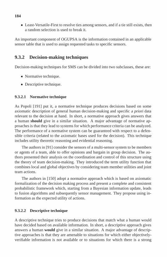
184

� Least-Versatile-First to resolve ties among sensors, and if a tie still exists, thena random selection is used to break it.

An important component of OGUPSA is the information contained in an applicablesensor table that is used to assign requested tasks to specific sensors.

9.3.2 Decision-making techniques

Decision-making techniques for SMS can be divided into two subclasses, these are:

� Normative technique.

� Descriptive technique.

9.3.2.1 Normative technique

As Popoli [191] put it, a normative technique produces decisions based on someaxiomatic description of general human decision-making and specific a priori datarelevant to the decision at hand. In short, a normative approach gives answers thata human should give in a similar situation. A major advantage of normative ap-proaches is that they lead to systems for which performance criteria can be analyzed.The performance of a normative system can be guaranteed with respect to a defen-sible criteria (related to the axiomatic bases used for the decision). This techniqueincludes utility theoretic reasoning and evidential reasoning.

The authors in [91] consider the sensors of a multi-sensor system to be membersor agents of a team, able to offer opinions and bargain in group decision. The au-thors presented their analysis on the coordination and control of this structure usingthe theory of team decision-making. They introduced the term utility function thatcombines local and global objectives by considering team member utilities and jointteam actions.

The authors in [150] adopt a normative approach which is based on axiomaticformalization of the decision making process and present a complete and consistentprobabilistic framework which, starting from a Bayesian information update, leadsto fusion algorithms and subsequently sensor management. They propose using in-formation as the expected utility of actions.

9.3.2.2 Descriptive technique

A descriptive technique tries to produce decisions that match what a human wouldhave decided based on available information. In short, a descriptive approach givesanswers a human would give in a similar situation. A major advantage of descrip-tive approaches is that they are amenable to situations for which either objectively-verifiable information is not available or to situations for which there is a strong

185

motive to make use of information that clearly is subjective. This technique includesfuzzy reasoning, fuzzy decision tree [191, 216] and knowledge-based approaches.

The essence of a descriptive approach is that the goal generally is to mimicexpert human behaviour for a particular problem domain. We simply hope to cap-ture the behaviour of a human faced with the same problem. The approaches differprimarily in their definition of how a problem should be solved rather than in theinformation used to solve it.

The thrust of normative approaches is to establish a formal decision-making cri-terion and remain faithful to it; the thrust of descriptive approaches is to provide asystem by which any human decision-making behaviour (whether or not it is for-mally consistent) can be easily codified. Descriptive approaches can be constructedon a weaker problem domain description than is required by a normative approach.

9.3.2.3 Hybrids of normative and descriptive techniques

As Denton et al. [67] put it, there is no single mathematical formalism that can beeffectively used to implement all of the required sensor management functions.

The authors in [25] discuss the issue that the choice of the algorithm used inthe determination of the ‘best’ sensor to perform a given service depends upon theservice in question. For example, the selection of the best sensor to perform a kine-matics track update employs a utility theory approach in which a numerical utility foreach sensor able to perform the update is computed, and the sensor with the highestutility is selected to perform the service. On the other hand, the selection of the bestsensor for the identification of services is performed by using a series of ‘If ... Then’rules.

9.3.2.4 Other decision-making tools

The author in [42] discusses the use of a neural network for sensor management. Thetask of the neural network is to predict the condition of the plant. This informationcan then be used to estimate the sensed data tolerance ranges at each operating con-dition for improved fault detection and isolation, hence help to improve the modelestimation of sensor values. The study has shown that a neural network is effective atboth recognizing the plant condition and in exploiting data redundancy, an intrinsicchallenge in the interdependencies of the sensed plant variables.

Hintz and McIntyre [100] present a methodology for quantifying the relativecontribution of specific sensor actions to a set of mission goals. They call the ap-proach goal lattices, since the mission goals and the ordering relationship applied toit can be represented as a lattice.

186

9.4 Sensor Management - Controller and Cueing

As highlighted in section 2, level 1 of the sensor management process involves con-trolling of the sensor action. Hence, conventional and advance control techniquesmay play a part in sensor management’s work at this level.

However, the process of control in SMS is not trivial [148]. Depending on thesystem involved, the SMS can be complicated by many factors, such as:

� Moving platforms.

� Geographical differences in sensor locations.

� Complexity in the fusion process.

� Complexity and different types of sensor systems.

The task of the controller can have many different functions or roles, such ascontrolling the:

� Sensor directions/pointing to best locate/identify the moving target.

� Sensor mode and when to switch mode.

� Sensor power level.

All the control tasks have the same objective, namely to improve the fusion process,such as in tracking and identifying the target. Figure 9.8 shows an example of apossible SMS behaving as a controller in a closed-loop form with the sensor systemand the fusion process.

With sensor manager providing command and control to the sensors, the sensorsystem will provide the fusion system with measurements, such as track data, and inturn the data fusion algorithm will provide the sensor manager with fused data.

However, the SMS is certainly more than just a controller. As discussed insection 2, there are different levels of processes in the SMS. One of this is the sensorcueing process.

Here, we define sensor cueing as taking the following two forms, namely:

� sensor hand-over and

� target acquisition with another sensor aiding.

The SMS may cue a sensor to hand over its current tracking target to anothersensor due to, say,

� another higher priority target entering its trackable region, or

187

� when the target is about to leave its trackable region.

The issue here is that SMS has to coordinate the handing over to ensure a smoothtransition and to reduce tracking or identification errors. On the other hand, a cuedtarget acquisition [30] process involves the SMS selecting which sensor to acquirethe target from and disseminating to that sensor the information required for suchacquisition. For example, the SMS may cue one of its radars to acquire range in-formation of a target that is being maintained primarily by an EO sensor (bearingonly).

Sensors vary greatly in their ability to detect the presence of targets or the onsetof a particular target behaviour. Therefore, sensor management may improve theresponse time of a sensor by a proper cueing process, hence obtaining informationfrom another sensor. Multiple sensors performance modelling or some expert rulescan be used for cueing to ensure no lost of target information.

In the next section, we demonstrate the SMS as a complete system based onwhat we have discussed in this section.

9.5 Simulation Results

In this experiment, we considered a 20km range (probability of detection 0:90)ground-based EO sensor with a field of view (FOV) of 15 degrees, and capable of apanning movement of 120 degrees. The tracking process takes place over a periodof 90 seconds.

Without the SMS, a normal EO sensor tracking a target will probably move at afixed panning rate, following the heading of the target.

In this simulation, the target moves at a constant velocity (20m=s) within thefirst 20 seconds, accelerates (5m=s2) between 21 and 50 seconds and decelerates(�5m=s2) from 51 and 90 seconds. Mid-way through the deceleration process, thetarget makes a right turn (time interval 65 to 73 seconds). An IMM filter is used inthe fusion process to track the target. The estimated target state is then sent to thesensor management system.

9.5.1 Fuzzy controller

The fuzzy controller used in the SMS has two inputs, namely error (k) and error (k�1), where error (k) represents the bearing error, in degrees, of the sensor boresightto the target at the kth time step. Note that this error(k) is obtained by taking theestimated bearing of the target minus the sensor boresight bearing.

The choice of error (k) as one of the input variables is intuitive. Nonetheless,most similar fuzzy control systems might use the rate of change of error or � error(k) as the second input variable, where � error(k) = error (k) - error (k � 1). The

188

time change in this simulation from k to k-1 is 1 second. From the above equation, itis clear that both pairs of error (k)/ � error(k) and error (k)/error (k�1) contain thesame amount of information and thus will provide equivalent inputs to the system.Our choice is based on simplification reasoning.

The crisp value of error (k) and error (k � 1) are mapped into five fuzzy sets,labelled in linguistic terms of: V L(very low), L (low), M (medium), H (high), andV H (very high).

The meaning of each linguistic term is determined by the specific membershipfunctions, which are defined by triangular functions on the universe of discourse oferror (k) and error (k � 1) respectively. Figures 9.5 and 9.6 show the input universeof discourse and the specific membership function.

The output of this fuzzy system is the panning rate (degree/sec) for the sensor,and its universe of discourse is divided into thirteen fuzzy sets labelled in the lin-guistic terms of: V L (very low), MVL (mid-very low), L (low), ML (mid-low),M (medium),MH (mid-high),H (high), MVH (mid-very high), V H (very high),MV VH (mid-very very high), V V H (very very high), MV V V H (mid-very veryvery high), and V V V H (very very very high). The membership functions are alsotriangular.

Figure 9.7 shows the output universe of discourse and the specific membershipfunctions.

The fuzzy system has a total of 25 IF-THEN rules, as summarized in table 9.1.A sample of these rules is given below.

� IF error(k � 1) is L AND error(k) is M THEN panning rate = VH.

� IF error(k � 1) is H AND error(k) is L THEN panning rate = ML.

� IF error(k � 1) is M AND error(k) is VL THEN panning rate = MVL.

e(k � 1)ne(k) VL L M H VHVL MVL ML MVVH MVVVH VVVHL MVL ML VH VVH VVVHM MVL ML VH VVH MVVHH MVL ML MVH MVVH MVVVH

VH MVL L H VH VVH

Table 9.1: The 25 fuzzy rules

where e(k) and e(k � 1) are the error(k) and error(k � 1) respectively. We usethe centre of gravity approach for the defuzzification process.

The complete closed-loop diagram is shown in Figure 9.8. The desired goal orthe set point of the SMS is to achieve zero error.

189

9.5.2 Example 1

In the first simulation, we considered one sensor. Figure 9.9 shows the target movingprofile, the sensor position and FOV. Figure 9.10 shows the results of the sensortracking error with respect to the target track with and without the sensor managedby the SMS.

With a fixed panning rate of about 1 degree per second, the sensor lost track ofthe target by the 11th time step and only managed to pick it up again on the 42nd,before losing it totally after the 51st. On the other hand, with a SMS, the sensormanaged to keep track of the target throughout the first 76 time steps. Note that dueto the limited panning angles of the EO sensor, regardless of whether the SMS is inuse, the sensor will not be able to sense the target beyond the 76th time step. Thisled us to the next example where 2 EO sensors are used for a better coverage.

9.5.3 Example 2

In this example, we introduce an additional EO sensor to the previous example. Acueing process is added to the SMS on top of the fuzzy controller. The position andcoverage of the two sensors are as shown in Figure 9.11.

Theoretically the sensor management cueing modules will command the nextsensor to take over when the target is within the sensor’s FOV. The cueing process isbased on a simple rule statement, as follows:

IFsensor 1 is within 10 degrees of its panning limits and target is withinsensor 2’s FOV,THENcue sensor 2 to take over the tracking process from sensor 1.

Alternatively,

IFanother target is entering the trackable region of Sensor 1, and Sensor1’s current target is within Sensor 2’s trackable region,THENcue Sensor 2 to take over the tracking process from Sensor 1.

Figure 9.12 shows the error output of the two sensors controlled by the SMS.The switch over occurred at the 62nd time step. Note that the errors correspond tothe target moving pattern.

190

9.6 Software Agents for Decentralized Sensor Man-agement

More recently, investigations are carried out using software agents to facilitate re-source allocation in a decentralized environment such as decentralized sensor net-work. The studies seek to use intelligent agents for the control of sensors in perform-ing various tasks, such as the tracking of a moving target, improve fusion processesthrough dynamic team formation and task allocation in a distributed/decentralizedenvironment.

Br�annstr�om [39] proposed an agent architecture, with mobile agents for a dy-namic sensor network. Agents were divided into different types according to theirroles and they communicated and cooperated closely with each other to ensure theproper functioning of the sensor network. In [206], an algorithm was proposed,using the metaphor of Belief-Desire-Intention (BDI), for the allocation of tasks toresources in a decentralized network, such that a task was assigned to a unique re-source. Each task has an agent attempting to bidding for the resources using the BDImetaphor. An arbitration agent or arbitrator, was used in the algorithm to determinethe agent’s intention that should be executed. In [212], the distributed task alloca-tion algorithm using computational geometry techniques were used. Soh et al. alsoprovided important insights into coalition formation for a time-critical and resource-constrained environment. It was acknowledged that in a multiagent system, whereagents have only local knowledge of the environment in which they are situated,optimal coalition formation is difficult. Thus, in such a time-critical system involv-ing the use of agents, it was more appropriate to trade-off sub-optimal solutions thatmet minimum requirements (satisfying coalitions) than seek to form coalitions thatachieved maximum performance.

However, there are also issues in using software agents for decentralized sensormanagement. For example, Howard et al. [105] raised the concern of negotiationamongst agents in a distributed sensor network may take too long for the coalition ofsensor agents to be useful in performing tasks. Hence, it may not be suitable for timecritical systems. Investigations are currently on-going in addressing some of theseissues.

9.7 Conclusions

We have presented the various classification and roles of sensor management. Theroles of sensor management as a controller were also discussed and demonstrated inthe simulation studies.

The sensor movement with the fixed panning rate will not be able to adapt totarget changes in direction and neither could they do a proper switching betweensensors. However, the sensor controlled by a properly designed SMS, such as the

191

fuzzy controller and the cue process, can adapt to a change in target movement anddetect the target.

There are, in general, more management issues for active sensors, such as thecontrol of the various active modes. Some examples of the active modes are burn-through modes, very high resolution modes, search mode and track mode. For pas-sive sensors, the management issues could be unique to each of the sensors. Ex-ample: sensor management could act as a feedback controller to control the passivesensor direction (e.g. adaptive scan rate), control the detection threshold or the timeintegration of the sensor’s data processing.

Lastly we discussed the use of software agents for decentralized sensor manage-ment.

192

0 0.5 1 1.5 2 2.5 3

0

0.2

0.4

0.6

0.8

1

Error(K−1)

Deg

ree

of m

embe

rshi

pVL L M H VH

Figure 9.5: Partition of the input universe of discourse for error (k).

0 0.5 1 1.5 2 2.5 3

0

0.2

0.4

0.6

0.8

1

Error(K)

Deg

ree

of m

embe

rshi

p

VL L M H VH

Figure 9.6: Partition of the input universe of discourse for error (k-1) .

193

0 0.5 1 1.5 2 2.5 3 3.5 4 4.5

0

0.2

0.4

0.6

0.8

1

Output

Deg

ree

of m

embe

rshi

p

VL MVL L ML M MH H MVH VH VVHMVVH VVVHMVVVH

Figure 9.7: Partition of the output universe of discourse.

signalcontrol

Sensor Manager

(controller + cue)Output (bearing)

estimated bearing

sensor boresight

data

+

-

bearing

error

(set point)

Desired goals

-

+

(IMM tracker)Fusion System

(EO sensors)

Sensor System

Figure 9.8: The complete closed-loop diagram.

194

0 1000 2000 3000 4000 5000 6000

−1000

−500

0

500

1000

1500

2000

2500

3000

3500

4000Flight Profile & Sensor FOV (Single Sensor)

Y P

ositi

on (

m)

X Position (m)

Target Moving PatternSensor Position Panning Angle Limits Center Axis FOV

Land Mass

Figure 9.9: Target moving profile and the sensor field of view (FOV).

0 10 20 30 40 50 60 70 80 90 100−25

−20

−15

−10

−5

0

5

10

15

20

25Graph of Bearing Error against Timestep (One Sensor)

Bea

ring

Err

or (

o )

Timestep (s)

Fixed Rate SMS−Fuzzy Controller

Figure 9.10: Error results of one sensor.

195

0 1000 2000 3000 4000 5000 6000

−1000

−500

0

500

1000

1500

2000

2500

3000

3500

4000Flight Profile & Sensor FOV (Two Sensors)

Y P

ositi

on (

m)

X Position (m)

Target Moving Pattern Sensor Positions Panning Angle Limits (Sensor 1)Panning Angle Limits (Sensor 2)

Land Mass

Figure 9.11: Position and coverage of the two sensors.

0 10 20 30 40 50 60 70 80 90 100−0.5

0

0.5

1

1.5

2

2.5Graph of Bearing Error against Timestep (Two Sensors)

Bea

ring

Err

or (

o )

Timestep (s)

Sensor 1Sensor 2

Switch Over

Figure 9.12: The error results of the two sensors with SMS.

Appendix A

A.1 Filter Models

A.1.1 Stationary model

� 1-D stationary model. For estimating the bearing of a target hovering or mov-ing at a constant bearing towards a sensor with zero mean random bearingvelocity. The following can be applied.

Xk+1 = Xk + Twk (A.1)

where: Xk = [xk], wk = [ _xk], and T is the sampling interval.

� 2-D stationary model. For estimating the position of a target at a stationary po-sition with zero mean random velocity. The model equation can be describedas:

Xk+1 = Xk + Twk (A.2)

where: Xk =

�xkyk

�, wk =

�_xk_yk

�, and T is the sampling interval.

A.1.2 Constant velocity model

� 1-D constant velocity model. For estimating the position of a target moving atconstant velocity with zero mean process noise.

Xk+1 =

�1 T0 1

�Xk +

�T 2

2T

�wk (A.3)

where: Xk =

�xk_xk

�

198

� 2-D constant velocity model. For estimating the position of a target movingat constant velocity motion with zero mean random acceleration. The modelequation can be described as:

Xk+1 =

2641 0 T 00 1 0 T0 0 1 00 0 0 1

375Xk +

2664

T 2

2 0

0 T 2

2T 00 T

3775wk (A.4)

where: Xk =

264xkyk_xk_yk

375.

A.1.3 Acceleration models

� 1-D acceleration model (Ramachandra’s model I). For estimating the positionof a vehicle moving at constant acceleration to a sensor with zero mean processnoise. The model equation is described as:

Xk+1 =

24 1 T T 2

20 1 T0 0 1

35Xk +

24 0

0ak

35 (A.5)

where: Xk =

24xk_xk

�xk

35.

And T is the sampling interval and ak is the process noise that disturbs theacceleration of the vehicle. It accounts for both maneuvering and other mod-eling errors, and is assumed to have zero mean and constant variance � 2

a:

The covariance matrix Q for the process noise is thus given by:

Q =

24 0 0 00 0 00 0 �2a

35 (A.6)

� 1-D acceleration model (Ramanchandra’s model II). The model can be definedby:

199

Xk+1 =

24 1 T T 2

20 1 T0 0 1

35Xk +

24 T 3

6T 2

2T

35wk (A.7)

where: Xk =

24xk_xk

�xk

35

� 2-D acceleration model (extension of Ramachandra’s model I).

Xk+1 =

26666664

1 0 T 0 T 2

2 0

0 1 0 T 0 T 2

20 0 1 0 T 00 0 0 1 0 T0 0 0 0 1 00 0 0 0 0 1

37777775Xk +

2666664

0 00 00 00 01 00 1

3777775wk (A.8)

where: Xk =

2666664

xkyk_xk_yk�xk�yk

3777775

A.1.4 Exponentially correlated velocity (ECV) model

In this model, it was assumed that the target velocity decays exponentially betweenmeasurements with no continuous process noise and undergoes an instantaneouschange at each sampling time.

Xk+1 =

�1 �(1� e��)0 e��

�Xk + Uk (A.9)

where: Xk =

�xk_xk

�.

Covariance of Uk is:

Q =

��2�2v [4e� 3� e�2� + 2�] ��2v [1� e��]2

��2v [1� e��]2 �2v [1� e�2�]

�(A.10)

where: � = T� , T is the sampling time and �2v is variance of the target velocity,

� is the target time.

200

The measurement model is:

Zk+1 = [ 1 0 ]Xk+1 + vk+1 (A.11)

where variance of vk is R = �2v .

A.1.5 Exponentially correlated acceleration (ECA) model

This model is applied to a vehicle moving with a random exponentially correlatedacceleration with a white noise process.

The model equation is:

Xk+1 =

24 1 T �2(� + e�� 1)0 1 �(1� e��)0 0 e��

35Xk + Uk (A.12)

where: Xk =

24xk_xk

�xk

35 and

T is the sampling time, � is the correlation time of the vehicle acceleration and� = T

� . The process noise covarianceQ is expressed as:

Q =

24 q11 q12 q13q12 q22 q23q13 q23 q33

35 (A.13)

where:q11 = �4�2a[1� e�2� + 2�(1� 2e�� + �2

3 )]q12 = �3�2a(1� e�� )2

q13 = �2�2a(1� e�2� � 2�e��)q22 = �2�2a[(1 + 2�)� (2� e��)2]q23 = ��2a(1� e��)2

q33 = �2a(1� e�2�)

and �2a is the variance of the target’s acceleration.

201

A.1.6 The coordinated turning model

Applicable to vehicle motion with a constant turn rate and constant speed.

Xk+1 =

2666641 sin!(k)T

!(k) 0 � 1�cos!(k)T!(k) 0

0 cos!(k)T 0 �sin!(k)T 0

0 1�cos!(k)T!(k) 1 sin!(k)T

!(k) 0

0 sin!(k)T 0 cos!(k)T 00 0 0 0 1

377775Xk +

266664

T 2

2 0 0T 0 00 T 2

2 00 T 00 0 T

377775 vk(A.14)

The measurement equation is thus:

Zk+1 =

�1 0 0 0 00 0 1 0 0

�Xk+1 +

�vx(k + 1)vy(k + 1)

�(A.15)

where: Xk =

26664x_xy_y!

37775

A.1.7 The measurement equation

The measurement equation converts state vector X to the measurement vector Z.For example, in 2-D constant velocity model, the measurement equation is:

Zk+1 =

�1 0 0 00 1 0 0

�Xk+1 +

�vx(k + 1)vy(k + 1)

�(A.16)

where:Zk+1 =

�xm(k + 1)ym(k + 1)

�.

And:xm(k + 1) = measured x coordinate at scan k + 1.ym(k + 1) = measured y coordinate at scan k + 1.vx(k + 1) = random noise on x measurement at scan k + 1.vy(k + 1) = random noise on y measurement at scan k + 1.

A.2 Generic Particle Filter

The dynamics system model of a manoeuvring target in a tracking system is givenby

_x = f(x; u; w) (A.17)

202

z(k) = h(x(k); v(k)) (A.18)

where x is the state vector, u is the control vector, w is the process noise vector rep-resenting possible deviations in f(:). z(k) is the discrete-time measurement vectorat time k, and v(k) is the measurement noise vector.

The dynamics of the target is a continuous-time process, as indicated by equationA.17. f(:) defines the motion for the target in a form of a differential equation. Themeasurement process is in discrete time because most sensors used for target trackingrecord the position and velocity at a given instance of time. Hence, the measurementequation A.18 in discrete form is

z(k) = H(k)x(k) + v(k) (A.19)

The function f(:) is usually unknown to the tracking system. Hence, the tar-get dynamics are commonly modelled by a deterministic linear dynamic system indiscrete time as follows:

x(k + 1) = F (k)x(k) +G(k)u(k) + w(k): (A.20)

At time k, x(k) (assumed to be a vector of dimension nx) is the state of the systemnormally containing the position and velocity of the target. F (k) is the transitionmatrix of dimensions (nx � nx) and it defines a linear constraint on the target dy-namics, u(k) is the unknown input control, a vector of dimension n u, G(k) is theinput gain (or noise matrix) (nx�nu matrix) and w(k) � N(0; Q(k)) is the processnoise which is usually assumed to be white Gaussian noise with variance Q.

In tracking manoeuvring targets, the control vector is not directly observable bythe tracking system. Since the input control is unknown, the dynamics model that isassumed for a target in a tracking system is further simplified as follows:

x(k + 1) = F (k)x(k) + w(k) (A.21)

The process noise w(k) can be used to model the unknown target acceleration.The unknown acceleration term can also be included in x to form a third-order model.However, the acceleration most often varies with time in such a manner that a modelcannot be clearly identified during tracking.

A.2.1 Generic particle filter algorithm

The following steps show the algorithm of the generic particle filter:

1. Initialization

� N = Number of particles.

� X(i)(1) = [x(1); y(1); 0; 0]T for i = 1; : : : ; N:

203

2. Prediction step

� For each particle i = 1; : : : ; N , evaluate the (k+1jk) state of the processsystem using the state at time k with the process noise at time k.

X(i)(k + 1jk) = F (k)X(i)(k) +

�Cauchy DistributedProcess Noise

�(k)

3. Evaluate importance weights

For each particle i = 1; : : : ; N ,

� Find the predicted observation state of the measurement system using thepredicted current state of the system and the measurement noise at timek.

z(i)(k + 1jk)=H(k + 1)X(i)(k + 1jk) +�Gaussian DistributedMeasurement Noise

�(k+1)

� Calculate the likelihood (importance weights) according to the distribu-tion given.

likelihood(i) = N (z(i)(k + 1jk); z(i)(k + 1); var) (A.22)

� Normalize the importance weights.

~w(i) =likelihood(i)PNj=1 likelihood

(j)(A.23)

4. Resampling/Selection

Resample using multinomial sampling techniques by multiplying the particleswith higher importance weights and suppressing the particles with lower im-portance weights. Modify the current state using the new indexed weightscalculated.

� Compute cumulative weights,

CumWt(i) =

iXj=1

~w(j) (A.24)

� Generate random variables uniformly distributed in U (i) � U(0; 1) withthe number of steps according to the number of particles.

204

� Determine which particle to multiply and which to suppress (see FigureA.1):For every particle inIndex i, where i = 1; : : : ; N

Case(1) : If 0 < U (i) < CumWt(1)

or

Case(2) : If CumWt(j) < U (i) < CumWt(j+1)

for j = 1; : : : ; N � 1. Replace the old inIndex of that particular particlei with the new outIndex of the CumWt, i.e. 1 for Case(1) or j + 1 forCase(2) and repeat for the next inIndex i = i+ 1.

resampled index

CumWt(i)

U(i)

(j)w(t)

j

i

N-1

Figure A.1: Resampling process.

5. Propagation step

� Incorporate the new state values after resampling of time step k for thecalculation of time step k + 1.

x(1:N)(k + 1jk + 1) = x(outIndex)(k + 1jk) (A.25)

� Compute posterior mean

x(k + 1) = mean[xi(k + 1jk + 1)]; for i = 1; : : : ; N (A.26)

� Repeat Step 2 to Step 5 for each time step.

205

A.3 Bayesian Classifier

The Bayesian classifier uses a probabilistic approach of updating the likelihood of ahypothesis given a previous likelihood estimate and new observation of the target ofinterest. An example of a classification hypothesis is ‘The target is of Type X’. Thewhole updating process is summarized by the following equation:

P (HijE) = P (EjHi)P (Hi)Pnj=1 P (EjHj)P (Hj)

for i = 1 : n (A.27)

whereP (HijE) : posterior probability of hypothesis H i being true, given the new

observationE, also known as the a posteriori probability.P (EjHi) : conditional probability of making observation E given that the

Hi is true, and it is also called the transitional probability; andP (Hi) : a priori probability of hypothesisHi being true.

Note that the n hypotheses H1; H2; : : : ; Hn must be mutually exclusive andexhaustive and

Pnj=1 P (Hj) = 1:

By the end of the updating process given an observation E, we obtain a set ofposterior probabilities of all the hypotheses. Commonly used decision logic will beto select the hypothesis with the largest posterior probability as the true hypothesis- this approach is known as the MAP (Maximum A Posteriori) method. In addition,most decision logic also requires this maximum posterior probability to exceed apredefined threshold before a declaration on the target’s classification is done.

However, in practical applications, a single observation usually will not lead tothe maximum posterior probability to exceed the given threshold, and usually severalobservational updates are needed to confirm the target classification.

The following equation is used instead of equation (A.27) given a sequential up-date of observations fE1; E2; : : : ; Ek�1; Ek; : : :g to update the posterior probabilityof each hypothesis at time step k:

P (HijEk) = P (Ek jHi)P (HijEk�1)Pnj=1 P (EkjHj)P (Hj jEk�1) for i = 1 : n: (A.28)

An important assumption here is that the observations are independent condi-tioned upon the same hypothesis. That is,

P (Ek; Ek�1jHi) = P (EkjHi)P (Ek�1jHi) 8k; i = 1 : n; (A.29)

although the observations are in general not independent, that is,

P (Ek; Ek�1) 6= P (Ek)P (Ek�1): (A.30)

206

{E1, E2, ... , Ek−1, Ek ...}Obervation Data

P(E k | Hi)

TransitionalProbabilities

P(H i)

PriorProbabilities

BayesianUpdate

P(H i) = P(H i | Ek)Update Prior Probabilites:

Decision Logic(MAP) + Threshold

Target Classification

Figure A.2: Sequential updating process of Bayesian classifier.

Figure A.2 depicts the sequential updating process of the Bayesian classifier.

Next, we consider the case of two sensors making a sequences of observa-tions fX1; X2; : : : ; Xk; : : :g and fY1; Y2; : : : ; Yk; : : :g, respectively. In this case,the Bayesian equation for the posterior probabilities updating becomes:

P (HijXk; Yk) =P (XkjHi)P (YkjHi)P (HijXk�1; Yk�1)Pnj=1 P (XkjHj)P (Yk jHj)P (Hj jXk�1; Yk�1)

for i = 1 : n:

(A.31)

As in equation (A.28), the assumption of independent observations being madeby Sensor 1 and Sensor 2 is in place. That is,

P (Xk; YkjHi) = P (XkjHi)P (Yk jHi) 8k; i = 1 : n: (A.32)

By applying equation (A.29), the classifier is effectively a joint classifier/fuserof two individual local classification processes, as depicted in Figure A.3.

Equation (A.29) can be easily generalized to handle cases of more than two

207

function

Sensor 2

m2 mass

LocalClassifier:

Sensor 1

m1 massfunction

LocalClassifier:

DS JointClassificationProcess:

Dempster Ruleof Combination

CombinedDeclarationof Target’sClassification

1 2 k ...}{Y , Y , ..., YObservationsSensor 2

{X1, X2, ..., Xk ...}

Sensor 1Observations

Figure A.3: Joint classification.

sensors.

A.4 Dempster-Shafer Classifier

The Dempster-Shafer classifier carries out evidential reasoning process using theDempster-Shafer theory developed by Shafer [207] and originally initiated by Demp-ster [207]. The Dempster-Shafer (DS) theory starts with a universal set:

� = fH1; H2; : : : ; Hng (A.33)

whose elements Hi are mutually exclusive and exhaustive. The set � is called theFrame of Discernment. In the case of classification application, the H i defined herecould be identical to those defined in the above Bayesian Classifier. However, thedifference here is that the attention is drawn onto the power set (the set of all subsets)of �, denoted by 2�, instead of the individualHi.

Ignorance

p(A) Pl(A)Bel(A)

Figure A.4: Belief and plausibility functions.

Let A be an element of 2�. We call A a proposition, where it is possibly a unionof some of the hypothesesHi.

208

Examples of A 2 2�:

A = fH2; H5g;A = fH3g;A = fH2; H3; H4; H6g;A = fH4; H5; H6g:

The DS reasoning consists of a basic probability mass assignment, which is afunction acting on the elements of the power set of �, m : 2� ! [0; 1], such that

m(�) = 0;XA��

m(A) = 1: (A.34)

A ‘belief function’ and a ‘plausibility function’ are associated with m, are de-fined as

Bel(A) =XB�A

m(b)

P l(A) =X

A\B 6=�

m(B) = a�Bel(A) (A.35)

respectively, for all A � � (Figure A.4).

The belief function provides a global measure of the belief that a proposition Ais true. On the other hand, the plausibility measure of proposition A is the amountof belief that could possibly be put on A if further evidence that support A arrives.Note thatBel(A) � P l(A), and the true probability ofA lies between them. The gapbetweenBel(A) and P l(A) denotes the classifier’s ignorance aboutA. In summary,the DS method distributes the total mass of uncertainty over all the subsets of �instead of over the individualHi.

The DS theory provides a rule called the Dempster’s Rule of Combination (alsocalled the orthogonal sum) to combine two mass functionsm1 andm2 and is definedas:

m1�m2(A) =

PB\C=Am1(B)m2(C)

1�K

K =X

B\C=�

m1(B)m2(C): (A.36)

The term K indicates the amount of conflicts between the two mass functions,and 1 � K is the re-normalizing term to ensure that the combined mass functionsatisfies condition (A.34). The orthogonal sum is associative and commutative.

209

{E1, E2, ... , Ek−1, Ek ...}Obervation Data

Assignm(A) base onnew evidence

ApplyDempster’s Ruleof Combination

PosteriorMassesm(A)

Pl(A) from updatedmasses

Compute Bel(A) and

Decision Logic(MAP) + Threshold

Massfunctions

Target Classification

Update

Figure A.5: DS classification process. Note that the update equation is givenby m(A) = (m(A)jEk)� (m(A)jEk�1)

The classification process of the individual sensor DS classifier is shown in Fig-ure A.5.

For a DS classifier, the choice of the decision logic is not as straight forwardas in the case of the Bayesian classifier. But the concept is still similar, as in itwe wish to select a proposition with the highest probability and check it against theclassification declaration threshold. What is tricky in this case is that:

� Firstly, we may want to decide on a single hypothesis and the set of proposi-tions consists of not only the singletons of the individual hypothesis, which isof the classifier’s main interest, but also all possible unions of them.

� Secondly, should the belief measure or the plausibility measure be used inthe judgement? In the literature, most researchers use the belief measure formaking decisions since it directly represents the amount of support given byall evidences available.

210

Smets [210] proposed an alternative approach as he introduced the Pignistic(from Latin pignus, meaning a bet) probability that transformed the belief functioninto a probability function for decision-making, and is defined as

BetP (Hi) =XHi2A

m(A)

jAj 8Hi 2 �: (A.37)

The idea is to distribute the ambiguous mass of a proposition equally over itselements.

The existence of the Dempster’s rule of combination also readily puts the DSclassifier as a suitable candidate to take on the role of the Joint Classifier, especiallywhen local classifiers output soft decisions that contain probabilistic measures of theconfidences of the hypotheses or propositions in question.

A.5 Artificial Immunology System

Biologists had studied the immune system, particularly the human immune system,for century. Recently, engineering researchers have been looking at the amazingand complex immunological defense mechanisms that make up the immune system.They are aiming at modeling or mimicking these mechanisms for practical appli-cations, such as: intelligent computer and network security systems, smart defensesystems, identification and pattern recognition systems, and general optimizationproblems.

Without the immune system the body would not be able to defend itself againstdisease and illness. The immune system consists of monocytes, which act as sen-tinels; helper and suppressor T-cells which sound the alarm; antibodies, killer cellsand cytotoxic T-cells which acts like an artillery; and macrophages which clean upthe battlefield [51]. The body is like a large battlefield where the immune system hasto ensure that it wins the battle 100% when invaded. When the immune system isfunctioning properly, we hardly notice the constant battles that rage within us.

The components of the human immune system are many and varied. The majorconstituents include the bone marrow, thymus, lymph nodes, spleen, tonsils, ap-pendix, Peyer’s patches and lymphatic vessels. These all protect the body againstdangerous toxins and invading microorganisms. Readers who are interested to knowmore about the artificial immune systems may refer to the book by Leandro N. deCastro and Jonathan Timmis [66].

A.5.1 B-cells or B- lymphocytes

B-cells or B-lymphocytes provide the antibodies or immunoglobulins to the body.They are precursors to the powerful plasma cells, which provide the body with valu-able antibodies or immunoglobulins. Antibodies constitute the immune system’s

211

single most powerful weapons. B-cells use antibodies as ammunition. For example,when a virus appears that is too strong for even the mighty macrophages, plasmacells launch antibodies, which, with the help of other immune cells, break the enemyto pieces.

Specialized training ensures that the B-cells have specific immunity to antigens.Antigens are foreign makers. It helps all immune cells differentiate invaders frombody cells. Approximately one billion B-cells in the body are sent for ‘training’ anddivided into groups. Depending on the group a B-cell is placed in, it will learn howto identify and kill one of a million different kinds of antigens that it may come intocontact with. This is the cell’s specific purpose, or its specificity. The B-cell will onlybe able to identify and confront that one specific antigen it specialized in. A healthybody produces enough B-cells to make the entire trained force a very effective armyagainst invaders that enter the body.

A.5.2 T-cell or T-lymphocytes

About 75% of the lymphocytes are trained in the thymus gland and are called T-cellsor T-lymphocytes. The T-cells do not use antibodies. Mature activated T-cells willevolve into one of the following kinds of cells: helper cells, suppressor cells, killercells, cytotoxic cells or memory cells.

Helper cells are responsible for prompting many of the immune system cellsinto action. It identifies an invader and rush to the spleen and lymph nodes where itsends chemical signals that stimulate other cells. By way of chemical signals calledlymphokines, the helper cells transmit messages that rally B-cells and macrophagesinto battle.

Suppressor cells suppress the activator messages sent out by the helper cells.This keeps the immune system from working too hard and killing many of its ownmembers.

Killer cells destroy cells which have penetrated the system and have been takenover by antigens. For example, when cancer takes over cells, the killer cell’s re-sponsibility is to destroy the occupied cell. Normally killer cells reside in the lymphnodes, but when antigens are present the killer cells swarm out to find the antigen oftheir specificity.

Cytotoxic cells also use poisons to kill the enemy. When cytotoxic cells comein contact with their target antigen, the cytotoxic cells release a cytotoxic substancethat either kills or renders the invader helpless.

Memory cells. Each time a B- or T-cell meets an invader, it memorizes its spe-cific qualities or makeup. This information is stored in the immune system, andnew lymphocytes recruits are trained to recognize this agent as an enemy. The nexttime the invader appears in the body, these memory cells identify it and begin theimmediate production of antibodies against it.

212

Lymph organs, such as lymph vessels and lymph nodes, aid the immune functionby cleansing the blood and organisms that are floating in the bloodstream.

A.5.3 What can we learn from the immune system?

Listed below are some possible areas where we can learn and attempt to engineerpossible algorithms for intelligent systems:

� Multi-layer defense mechanism. The complete immune system is a multi-layer defense mechanism. The first layer of defense in an immune system isthe physical barrier, namely the skin, nasal hairs and mucous tissues. Itchingeffects that cause coughing and sneezing help to expel the invader. The sec-ond layer of defense is the biochemical barrier, such as fluids (saliva, sweatand tears), that contain destructive enzymes. Stomach acids will kill mostmicroorganisms ingested in food and drinks. The third layer of defense areorgans such as the lymph node and spleen (also see the adaptive immune sys-tem). These contain a system of passages through which lymph and bloodcirculate constantly. In this way harmful elements can be removed from theblood and lymphs before they have the opportunity to multiply. The completeimmune systems are on constant ‘seek and destroy’ mission.

� Attack mechanism. The immune system’s strategic attack may be divided intothree phases. These are: recognition of the antigen, activation of lymphocytesand effector phase.

� Pattern recognition mechanism. By direct matching of pattern. New patternwill be learnt and adaptively modeled for future matching.

� Specialized function. The B-cell and the several groups of T-cells have spe-cialized functions. Each plays a role in destroying a particular invader.

� Working cooperatively. The complete immune system works together to battleagainst a multitude of pathogens. For example, one can see helper cells asthe ‘bugler’ giving call to arm for battle. Protein emissions from helper cellsactually tell B-cells to begin transformation into plasma cells. The plasmacells, together with other immune cells, break the pathogen. This complexcollaboration process continues until all the foreign invaders are destroyed.

� Decentralized control. The components of the immune system are decentral-ized and spread across the entire body. It is not controlled by a central organ.Each component of the immune system act autonomously in identifying andeliminating the pathogens. The lymphoid organs are distributed throughoutthe body. These are subjected to decentralized ‘training’ in the ‘instructioncenter’, such as the thymus gland and lymphoid tissues.

213

� Adaptation mechanism. The immune system can adapt itself structurally andin numbers to the invaders’ challenges. It has the capabilities to learn andremember the identification of the invaders, and to clone itself in large numberswhen challenged.

A.6 Introduction To Ontology

Lately, there has been a lot of interest in ontologies, partly due to the interest inthe semantic web and partly because ontologies promise to be a means of achievingsemantic interoperability between different systems. In this section, we examine thebackground and the components of an ontology and also highlight aspects of theirdevelopment and reasoning processes.

A.6.1 Introduction

In May 2001, Tim Berners-Lee (the founder of the Web) shared his vision of thefuture in a Scientific American article entitled ‘The Semantic Web’ [24]. His vi-sion was ‘an extension of the current web in which information is given well-definedmeaning’ that computers or software agents can understand and utilize in performingcomplex tasks. For instance, an agent can arrange on behalf of its user an appoint-ment with a specialist by understanding the meaning of the various information itis presented with; like medical condition, doctor’s schedule and location of clinics.The well-defined meaning or semantic is provided by ontologies, leading some re-searchers to conclude ‘ontologies are the basic infrastructure for the Semantic Web’[151].

An ontology is an artifact built using formal languages that allows the inten-sion of the words used by a community, when they communicate, to be defined asprecisely as possible. When the community speaks of a certain object or a certainthought, they hold in their mind certain concepts that are not expressed in the utter-ances they make. For instance the concept of ‘ABOVE’ encompasses many differentconfiguration of objects, all of which is understood to exhibit the ‘ABOVE’ relation-ship as shown in Figure A.6. For an ‘ABOVE’ relation, definitions can include thenotion of contact or lack of contact as well as the extent of area being encompassed.An ontology seeks to make these hidden concepts explicit, necessitating its users andbuilders to provide definitions that are unambiguous and as close to the intension ofthe concepts as possibly allowed by the limitations of the formal language.

A.6.2 Components of ontologies

An ontology has four elements: concept, instance, relation and axiom. Each ontol-ogy talks about concepts and their instantiations. Concepts can be seen as a cate-

214

(a) (b) (c)

Object

Table

Figure A.6: Different interpretations of the ‘ABOVE’ relation.

gorization of the domain into different categories that may or may not overlap. Anindividual or instance is said to belong to a concept if it embodies the characteristicsof the concept. In our simple ontology (see Figure A.7), we have four concepts:human beings, male human beings, female human beings and apples. We also havetwo individuals, John who is a male human being and Mary who is a female humanbeing.

AppleHuman

Female_HumanMale_Human

John Mary

Axiom − Male_Humandisjoint_with Female_Human

Instance_of

Is_A Is_A

Instance_of

Eats

Sells

Figure A.7: Simple Ontology.

Relations and axioms differentiate an ontology from a simple lexicon. A rela-tion describes how concepts and instances are associated. In our simple ontology,human beings is related to male human beings and female human beings by the Is Aor subsumption relation. This means that instances of male human beings share allthe characteristics on human beings and, similarly, instances of female human beingsshare all the characteristics of the parent concept. Human beings are related to apples

215

via the EAT relationship denoting the idea that apples function as food for human be-ings as well as via the SELLS relationship. There can be any number of relationshipsdefined between any pair of concepts. An axiom is also included in this ontology.The concept of male human beings is disjoint from the concept of female human be-ings showing that these two concepts do not share common instances. Every axiomshapes an ontology closer to the intended expression of the conceptualisation. In thisparticular example, we are excluding from consideration androgynous human beings(i.e. human beings born with either both male and female sex organs).

A.6.3 Classification of ontologies

An ontology can be classified into one of three roles: top-level, domain and applica-tion. These is not static classification, as a top-level ontology for a group of systemsmay be an application ontology of a different group of systems. In general, a top-level ontology provides broad definitions that can be used across several domains.An application ontology is a specific ontology that may be irrelevant to another ap-plication as it describes constraints that applies to the application.

The choice of the language used to encode the ontology, as well as the targetlevel of the ontology, determines its expressiveness. In general, the more expressiveis an ontology, the harder and longer it is to reason with the ontology. Borgida andPatel-Schneider illustrated the difficulty with an example [38]. In the application,ontologies are used as terminological services, allowing constraints between terms tobe checked during its execution. These ontologies would have limited expressivenessso as to reduce the computational requirements for the reasoning task. Ontologiesused as references for a discourse are much more expressive since the requirementsfor reasoning tasks are fewer, i.e. the ontologies are used to establish consensusabout the semantics of the terms used and not to infer new knowledge.

A.6.4 Principles of ontology design

Gruber articulated five design principles for good ontology design [90] that we candistill into two: clarity and modularity. A good ontology would be clear to its de-signers, users and also to the machines. The purpose of the ontology would bedocumented and the ontological entities described in a clear way that it is obvi-ous, i.e. what and how each term is used. Each term is defined concisely andcomprehensively. Any ambiguous term should be renamed so that the ambiguitycan be resolved. For instance, BANK can be interpreted as a financial institutionor as a geographic feature. In this case, we should name the term so that thesecharacteristics are clear in the names (e.g. BANK-FINANCIAL-INSTITUTION,BANK-GEOGRAPHIC-FEATURE). Relationships and formal semantic should alsobe stated, if possible, in order to provide further clarity to the terms.

Like good software engineering practice, an ontology should also be developed

216

as smaller, internally coherent components (or modules). A smaller ontology tendsto be self-contained and easier to reuse than a larger, more monolithic ontology sinceit has less ontological commitments. The complexity of building an ontology is alsomanaged by focusing on the development of smaller modules and the integration ofthe modules into the desired ontology.

A closely-related concept to modularity is extensibility. While developing theontology, we should bear in mind its future extensions. An ontology should not betoo generic nor should it be overly specific. In other words, it should be well tailoredto its purpose and domain.

An ontology can be represented in different languages (e.g. frame, first-orderlogic, etc.) The chosen ontology representation language should be flexible enoughthat the ontology can be readily translated to a different application implementationlanguage (e.g. C++/Java classes, production rules). This would allow the designedontology to have minimal encoding bias. The DARPA Agent Markup Languagewith the Ontology Inference Layer (DAML+OIL) is based on a family of restrictedfirst-order logics known as Description Logics that provides the formal foundation.We are able to perform reasoning through a variety of tools like the Java TheoremProver (JTP) [83], Jena API [154] and Z/Eves with DAML+OIL semantic library[70]. Using this language also has an advantage - as a migration path from theUniversity of Maryland (http://www.mindswap.org) exists to transform ontologieswritten in DAML+OIL to the upcoming standard W3C Web Ontology Language.

A.6.5 Conclusion

In summary, an ontology encodes knowledge in a formal language that can be usedto establish consensus among a community of users, as well as to be processed by acomputer or software agent in its reasoning task. An ontology consists of concepts,instances, relations and axioms, whose development are guided by two principles:clarity and modularity.

Bibliography

[1] D. H. Ackley, G. E. Hinton, and T. J. Sejnowski. A learning algorithm forboltzmann machines. Cognitive Science, 9:147–169, 1985.

[2] S. V. B. Aiyer, M. Niranjan, and F. Fallside. A theoretical investigation into theperformance of the Hopfield model. IEEE Transactions on Neural Networks,1(2):204–215, June 1990.

[3] L. B. Almeidal. A learning rule for asynchronous perceptron with feedbackin a combinatorial environment. Proceedings of the IEEE First InternationalConference on Neural Networks, 2:609–618, 1987.

[4] A. T. Alouani, N. Auger, and T. R. Rice. On the generalized nearest neighborfilter. In 22nd Southeastern Symposium on System Theory, pages 261–264.IEEE Computer Society Press, 11-13 March 1990.

[5] A. T. Alouani and T. R. Rice. Multiple model tracking with feedback. SignalProcessing, Sensor Fusion, and Target Recognition X, Proceedings of SPIE,4380:13–24, April 2001.

[6] P. E. An and C. J. Harris. Multi-dimensional locally generalizing neural net-works for real time control. In H. B. Verbruggen and M. G. Rodd, editors, Ar-tificial Intelligence in Real-Time Control 1992 IFAC Symposia Series, pages87–91. Pergamon Press, Delft, The Netherlands, 1993.

[7] S. L. Andresen. Herbert A. Simon: AI Pioneer. IEEE Intelligent Systems,16(4):71–74, July/August 2001.

[8] A. Averbuch, S. Itzikowitz, and T. Kapon. Radar target tracking - Viterbiversus IMM. IEEE Transactions on Aerospace and Electronic Systems,27(3):550–563, May 1991.

[9] V. V. Badami and N. W. Chbat. Home appliances get smart. IEEE Spectrum,pages 36–43, August 1998.

[10] Y. Bar-Shalom. Multitarget-Multisensor Tracking: Advanced Applications.Artech House, Inc, 1990.

218

[11] Y. Bar-Shalom. Tracking of splitting targets in clutter using an interactingmultiple model joint probabilistic data association filter. In Proceeding of the30th Conference on Decision and Control, pages 2043–2048. IEEE, Brighton,England, December 1991.

[12] Y. Bar-Shalom. Multitarget-Multisensor Tracking: Applications and Ad-vances, volume 2. Artech House, Inc, 1992.

[13] Y. Bar-Shalom and L. Campo. The effect of common process noise on thetwo-sensor fused track covariance. IEEE Transactions on Aerospace andElectronic Systems, AES-22:803–805, Nov 1986.

[14] Y. Bar-Shalom, K. C. Chang, and H. A. P. Blom. Tracking of splitting targetsin clutter using an interacting multiple model joint probabilistic data associa-tion filter. In Multitarget-Multisensor Tracking: Applications and Advances,chapter 4, pages 93–110. Artech House, 1992.

[15] Y. Bar-Shalom, H. Chen, and T. Kirubarajan. Performance limits of track-to-track fusion vs. centralized estimation: Theory and application. Fusion 2001,1, August 2001.

[16] Y. Bar-Shalom and T. E. Fortmann. Tracking and Data Association, volume179 of Mathematics in Science and Engineering. Academic Press, Orlando,Florida, 1988.

[17] Y. Bar-Shalom and X. R. Li. Estimation and tracking: Principles, Techniquesand Software. Artech House, Inc, 1993.

[18] Y. Bar-Shalom and X. R. Li. Multitarget-Multisensor Tracking: Principlesand Techniques. Lecture Notes. YBS Publishing, Storrs (CT 06269-3157),1995.

[19] Y. Bar-Shalom and G. D. Marcus. Tracking with measurements of uncertainorigin and random arrival times. IEEE Transactions on Automatic Control,25:802–807, August 1980.

[20] Y. Bar-Shalom and E. Tse. Tracking in a cluttered environment with proba-bilistic data association. Automatica, 11:451–460, September 1975.

[21] A. G. Barto, R. S. Sutton, and C. W. Anderson. Neuronlike adaptive ele-ments that can solve difficult learning control problems. IEEE Transactionson Systems Man and Cybernetics, 13(5):834–846, September/October 1983.

[22] R. Beale and T. Jackson. Neural Computing: an introduction. Institute ofPhysics Publishing, 1990.

[23] T.M. Berg and H. Durrant-Whyte. Distributed and decentralized estimation.Proceedings of the International Conference on Intelligent Control and In-strumentation, 2:1118–1123, Feb 1992.

219

[24] T. Berners-Lee, J. Hendler, and O. Lassila. The semantic web. ScientificAmerican, pages 34–43, 2001.

[25] S. G. Bier, P. L. Rothman, and R. A. Manske. Intelligent sensor managementfor beyond visual range air to air combat. Proceedings of the IEEE 1988National Aerospace and Electronics, 1:264–269, May 1988.

[26] K. Birmiwal and Y. Bar-Shalom. On tracking a maneuvering target in clutter.IEEE Transactions on Aerospace and Electronic Systems, 20:635–644, Sept1984.

[27] H. Bischof. Pyramidal Neural Networks. Lawrence Erlbaum Associate Inc.,1995.

[28] K. K. Biswas and A. K. Mahalanabis. Optimal fixed-lag smoothing for timedelayed system with colored noise. IEEE Transactions on Automatic Control,17:387–388, 1972.

[29] S. Blackman, R. Dempster, and T. Broida. Multiple hypothesis track confir-mation for infrared surveillance systems. IEEE Transactions on Aerospaceand Electronic Systems, 29(3):810–824, July 1993.

[30] S. Blackman and R. Popoli. Design and Analysis of Modern Tracking Systems.Artech House, 1999.

[31] S. S. Blackman. Multiple-target tracking with radar applications. ArtechHouse, 1986.

[32] W. D. Blair and G. A. Watson. Interacting multiple bias model algorithm withapplication to tracking maneuvering targets. In Proceedings of the 31st Con-ference on Decision and Control, pages 3790–3795. IEEE, 16-18 December1992.

[33] W. D. Blair, G. A. Watson, and T. R. Rice. Interacting multiple model filter fortracking maneuvering targets in spherical coordinates. In IEEE proceedingsof the SOUTHEASTCON’91, volume 2, pages 1055–1059. IEEE, 7-10 April1991.

[34] W. D. Blair, G. A. Watson, and T. R. Rice. Tracking maneuvering targetswith an interacting multiple model filter containing exponentially-correlatedacceleration models. In System Theory, Proceedings, pages 224–228. IEEEComputer Society Press, 10-12 March 1991.

[35] B. Blake. Jane’s Radar and electronic Warfare systems. An InternationalThomson Publishing Company, 1995-96.

[36] A. Blum. Neural Networks in C plus plus: An object-oriented framework forbuilding connectionist systems. New York: Wiley, 1992.

220

[37] G. Booch, J. Rumbaugh, and I. Jacobson. The Unified Modeling LanguageUser Guide. Addison Welsey, 1998.

[38] A. Borgida and P. F. Patel-Schneider. A semantics and complete algorithm forsubsumption in the classic description logic. Journal of Artificial IntelligenceResearch, 1:277–308, 1994.

[39] M. Br�annstr�om and E. Jungert. A scalable agent architecture for a dynamicsensor network. Fundamenta Informaticae, XXI:1–13, 2002.

[40] E. A. Bretz. Transportation. IEEE Spectrum, 36(1):98–103, Jan 1999.

[41] D. S. Broomhead and D. Lowe. Multivariable functional interpolation andadaptive networks. Complex System, 2:321–355, 1988.

[42] T. A. Brownell. Neural networks for sensor management and diagnostics. Pro-ceedings of the IEEE 1992 National Aerospace and Electronics Conference,3:923–929, May 1992.

[43] D. M. Buede and E. L. Waltz. Issues in sensor management. In Proceedingsof the 5th IEEE International Symposium on Intelligent Control, volume 2,pages 839–842. IEEE Computer Society Press, September 1990.

[44] B. H. Cantrell, G. V. Trunk, F. D. Queen, J. D. Wilson, and J. J. Alter. Au-tomatic detection and integrated tracking. IEEE International Radar Confer-ence, pages 391–395, 1975.

[45] A. Carling. Introducing Neural Networks. John Wiley and Sons, 1992.

[46] M. Cellario. Human-centered intelligent vehicles: Toward multimodal inter-face integration. IEEE Intelligent Systems, 16(4):78–81, July/August 2001.

[47] C. W. Chan. Cognitive informatics: a knowledge engineering perspective.Proceedings of the First International Conference on Cognitive Informatics,2002.

[48] K. C. C. Chan, V. Lee, and H. Leung. Robust target tracking using a fuzzy fil-ter. IEEE International Conference on System, Man and Cybernetics, 5:4464–4467, 1995.

[49] K. C. Chang and Y. Bar-Shalom. Joint probabilistic data association for multi-target tracking with possibly unresolved measurements and maneuvers. IEEETransactions on Automatic Control, 29:585–594, July 1984.

[50] J. Chen, H. Leung, T. Lo, J. Litva, and M. Blanchette. A modified probabilis-tic data association filter in real clutter environment. IEEE Transactions onAerospace and Electronic Systems, 32:300–313, 1996.

[51] J. F. Chen. Plant Foods and Nutritional Immunology: A Scientific Approach.Bright Ideas Press, Provo, UTAH, USA, 1996.

221

[52] M. Chester. Neural Networks - A Tutorial. Prentice Hall International, 1993.

[53] E. H. Chi and S. K. Card. Sensemaking of evolving web sites using visualiza-tion spreadsheets. IEEE, pages 18–25, 1999.

[54] V. Chiew. A software engineering cognitive knowledge discovery framework.Proceedings of the First IEEE International Conference on Cognitive Infor-matics, 2002.

[55] L. Chin. Application of neural networks in target tracking. IEEE Transactionson Aerospace and Electronic Systems, 30(1):281–287, January 1994.

[56] C. Y. Chong and S. Mori. Convex combination and covariance intersectionalgorithms in distributed fusion. Fusion 2001, 1, August 2001.

[57] C. K. Chui and G. Chen. Kalman Filtering. Springer Series in InformationSciences. Springer-Verlag, 1987.

[58] A. Cichocki and R. Unbehauen. Neural Networks for Optimization and SignalProcessing. John Wiley and Sons, 1993.

[59] S. A. Cohen. Adaptive variable update rate algorithm for tracking targets witha phased array radar. IEE Proceedings, Pt F, 133(3):277–280, June 1986.

[60] M. L. Cone and S. Musick. Scheduling for sensor management using geneticsearch. Proceedings of the IEEE 1996 National Aerospace and ElectronicsConference, NAECON 1996, 1:150–156, May 1996.

[61] D. J. Cook, P. Gmytrasiewicz, and L. B. Holder. Decision-theoretic cooper-ative sensor planning. IEEE Transactions on Pattern Analysis and MachineIntelligence, 18(10):1013–1023, October 1996.

[62] G. Cybenko. Approximation by superposition of a sigmoidal function. Math-ematical Control, Signal and Systems, 2:303–314, 1989.

[63] E. Daeipour and Y. Bar-Shalom. An interacting multiple model approachfor target tracking with glint noise. IEEE Transactions on Aerospace andElectronic Systems, 31(2):706–715, April 1995.

[64] R. Danchick and G. E. Newnam. A fast method for finding the exact N-besthypotheses for multitarget tracking. IEEE Transactions on Aerospace andElectronic Systems, 29(2):555–560, April 1993.

[65] J. E. Dayhoff. Neural Network Architectures. Van Nostrand Reinhold, 1990.

[66] L. N. de Castro and Jonathan Timmis. Artificial Immune Systems: A newcomputational intelligence approach. Springer-Verlag, 2002.

[67] R. V. Denton, E. I. Alcaraz, J. Llinas, and K. J. Hintz. Towards modern sensormanagement systems. Science of Command and Control, Part 3 Coping withChange:119–134, 1994. AFCEA International Press.

222

[68] J. DeVilliers and E. Barnard. Backpropagation neural nets with one and twohidden layers. IEEE Transactions on Neural Networks, 4(1):136–141, January1993.

[69] P. DeWilde. Neural Networks Models: An Analysis. London: Springer, 1996.

[70] J. S. Dong, J. Sun, and H. Z. Wang. Approach to semantic web. Proceedings ofthe International Conference on Formal Engineering Methods (ICFEM’02),pages 156–167, 2002.

[71] H. Durrant-Whyte, B. Grocholsky, and P. Gibbons. An information theoreticapproach to decentralized control of multiple autonomous flight vehicles. Sen-sor Fusion and Decentralised Control in Robotic Systems III, Proceedings ofSPIE, 4196:337–347, 2000.

[72] H. Durrant-Whyte and J. Manyika. Data Fusion and Sensor Management: adecentralized information theoretic approach. Ellis Horwood Limited, 1994.

[73] H. Durrant-Whyte, B.S.Y. Rao, and H. Hu. Towards a Fully DecentralizedArchitecture for Multisensor Data Fusion. University of Oxford Departmentof Engineering Science, 1991.

[74] H. Durrant-Whyte and M. Stevens. Data fusion in decentralized sensing net-works. Fusion 2001, 1, August 2001.

[75] J. L. Elman. Finding structure in time. Cognitive Science, 14:179–211, 1990.

[76] S. E. Fahlman. Faster-learning variations on back-propagation: An empiricalstudy. In D. S. Touretzky, editor, Proceedings 1988 Connectionist ModelsSummer School, pages 38–51. Morgan-Kaufman, Pittsburgh, 1988.

[77] L. Fausett. Fundamentals of Neural Networks. Prentice-Hall International,1994.

[78] R. Fitzgerald. Development of practical JPDA logic for multitarget trackingby microprocessor. In Multitarget-Multisensor tracking: Advanced Applica-tions, pages 1–23. Artech House, 1990.

[79] L. J. Fogel, A. J. Owen, and M. J. Walsh. Artificial Intelligence throughSimulated Evolution. John Wiley, 1966.

[80] A. C. M. Fong and S. C. Hui. An intelligent online machine fault diagnosissystem. Computing and Control Engineering Journal, 12(5):217–223, Octo-ber 2001.

[81] T. E. Fortmann. Detection thresholds for multi-target tracking in clutter. InProceedings of the 1981 IEEE Conference on Decision and Control, pages1401–1408, 16-18 December 1981.

223

[82] T. E. Fortmann, Y. Bar-Shalom, and M. Scheffe. Sonar tracking of multipletargets using joint probabilistic data association. IEEE Transactions on OceanEnvironments, 8:173–184, July 1983.

[83] G. Frank. A general interface for interaction of special-purpose reasonerswithin a modular reasoning system. Proceedings of the AAAI Fall Symposium,pages 57–62, 1999.

[84] J. A. Freeman and D. M. Skapura. Neural Networks Algorithms, Applications,and Programming Techniques. Addison-Wesley, 1992.

[85] L. M. Fu. Neural Networks in Computer Intelligence. London:McGraw-Hill,1994.

[86] K. Funahashi. On the approximation realization of continuous mappings byneural networks. Neural Networks, 2:183–192, 1989.

[87] K. Funahashi and Y. Nakamura. Approximation of dynamical systems by con-tinuous time recurrent neural networks. Neural Networks, 6:801–806, 1993.

[88] J. J. Grefenstette. Optimization of control parameters for genetic algorithms.IEEE Transactions on systems, Man and Cybernetics, 16(1):122–128, 1986.

[89] S. Grossberg. Classical and instrumental learning by neural networks. InProgress in theoretical biology, volume 3, pages 51–141. New York, Aca-demic Press, 1974.

[90] T. R. Gruber. A translation approach to portable ontology specifications.Knowledge Acquisition, 5:199–220, 1993.

[91] G. Hager and H. F. Durrant-Whyte. Information and multi-sensor coordina-tion. Uncertainty in Artificial Intelligence, 2(381-394), 1988.

[92] D. Hall. An introduction to multisensor data fusion. TechReach Inc, 1998.

[93] D. L. Hall. Mathematical Techniques in Multisensor Data Fusion. ArtechHouse, 1992.

[94] K. M. Harmeyer and K. C. Wetzel. Brain research and implications for engi-neering education. IEEE, FIE’96 Proceedings, pages 466–470, 1996.

[95] S. Haykin. Neural Networks - A comprehensive foundation. Macmillan Col-lege Publishing Company, Inc., 1994.

[96] D. O. Hebb. The organisation of behavior. Wiley, New York, 1949.

[97] R. Hecht-Nielsen. Neurocomputing. Addison-Wesley, 1990.

[98] B. J. Hellstrom and L. N. Kanal. Knapsack packing networks. IEEE Transac-tions on Neural Networks, 3(2):302–307, March 1992.

224

[99] J. Hertz, A. Krogh, and R. G. Palmer. Introduction to the Theory of NeuralComputation. Addison-Wesley, 1991.

[100] K. J. Hintz and G. McIntyre. Goal lattices for sensor management. Proceed-ings of SPIE, Signal Processing, Sensor Fusion, and Target Recognition VIII,3720-25:249–255, April 1999.

[101] J. H. Holland. Adaptation in natural and artificial systems. Ann Ar-bor:University of Michigan press, 1975.

[102] J. J. Hopfield. Neural networks and physical systems with emergent collectivecomputational abilities. Proceedings National Academy of Sciences, 79:2554–2558, 1982.

[103] K. Hornik. Multilayer feedforward networks are universal approximators.Neural Networks, 2(5):359–366, 1989.

[104] K. Hornik. Approximation capabilities of multilayer feedforward networks.Neural Networks, 4(2):251–257, 1991.

[105] M. Howard, D. Payton, and R. Estkowski. Coalitions for distributed sensorfusion. Proceedings of 5th Annual Conference on Information Fusion, 2002.

[106] M. B. Ignagni. Separate-bias kalman estimator with bias state noise. IEEETransactions on Automatic Control, 35(3):338–341, December 1990.

[107] R. A. Iltis and P. Y. Ting. Data association in multi-target tracking: A solutionusing a layered Boltzmann machine. In Proceeding IJCNN’91, volume 1,pages 31–36. IEEE, 1991.

[108] R. A. Iltis and P. Y. Ting. Computing association probabilities using parallelboltzmann machines. IEEE Transactions on Neural Networks, 4(2):221–233,March 1993.

[109] S. S. Iyengar, D. N. Jayasimha, and D. Nadig. A versatile architecture forthe distributed sensor integration problem. IEEE Transaction on Computer,43(2):175–185, February 1994.

[110] R. A. Jacobs. Increased rates of convergence through learning rate adaptation.Neural Networks, 1:295–307, 1988.

[111] T. W. Jeffrey. Track quality estimation for multiple-target tracking radars. InProceedings of the 1989 IEEE Radar Conference, pages 76–79. IEEE, Mar1989.

[112] N. R. Jennings, P. Faratin, A. R. Lomuscio, S. Parsons, C. Sierra, andM. Wooldridge. Automated negotiation : Prospect, methods and challenges.International Journal of Group Decision and Negotiation, 10(2):199–215,2001.

225

[113] N. R. Jennings, K. Sycara, and M. Wooldridge. On agent-based softwareengineering. Artificial Intelligence, 117(2):277–296, 2000.

[114] L. Jin, P. N. Nikiforuk, and M. M. Gupta. Approximation of discrete-timestate-space trajectories using dynamical recurrent neural networks. IEEETransactions on Automatic Control, 40(7):1266–1270, July 1995.

[115] W. D. Jones. Keeping cars from crashing. IEEE Spectrum, September 2001.

[116] H. Jung, M. Tambe, and S. Kulkarni. Argumentation as distributed constraintsatisfaction : Applications and results. Proceedings of the 5th InternationalConference on Autonomous Agents, July 2001.

[117] P. R. Kalata. The tracking index: A generalized parameter for �-� and �-�- target trackers. IEEE Transactions on Aerospace and Electronic Systems,20(2):174–182, March 1984.

[118] G. Kaufman. Sensitive snakes offer thermal expertise. DefenseNews, page 4,May 27 - June 2 2002.

[119] S. S. Keerthi and B. Ravindran. A tutorial survey of reinforcement learn-ing. Sadhana Academy Proceedings in Engineering Sciences, 19(6):851–889,1994.

[120] J. Kim, Y. Moon, and B. P. Zeigler. Designing fuzzy net controllers usinggenetic algorithms. IEEE Control Systems, 15(3):66–72, June 1995.

[121] L. A. Klein. Sensor and Data Fusion Concepts and Applications. SPIE Opti-cal Engineering Press, 1993.

[122] L. A. Klein. Sensor and Data Fusion Concepts and Applications. SPIE Opti-cal Engineering Press, 1999. Second Edition.

[123] T. Kohonen. Self-organised formation of topologically correct feature maps.Biological Cybernetics, 43:59–69, 1982.

[124] J. F. Kolen and J. B. Pollack. Back propagation is sensitive to initial condi-tions. In R. P. Lippmann, S. E. Moody, and D. S. Touretzky, editors, Advancesin Neural Information Processing Systems Volume 3, pages 860–866. San Ma-teo: Morgan Kaufmann, 1990.

[125] G. A. Korn. Neural Networks and fuzzy-logic control on personal computerand workstation. The MIT Press, London, 1995.

[126] B. Kosko. Bidirectional associative memories. IEEE Transactions on SystemsMan and Cybernetics, 18(1):49–60, January/February 1988.

[127] E. B. Kosmatopoulos, M. M. Polycarpou, M. A. Christodoulou, and P. A.Ioannou. High-order neural network structures for identification of dynamicalsystems. IEEE Transactions on Neural Networks, 6(2):422–431, 1995.

226

[128] Y. Kosuge. Maneuvering target tracking using multiple maneuver modeljoint probabilistic data association. In Proceedings IECON’91. 1991 Inter-national Conference on Industrial Electronics, Control and Instrumentation,pages 2059–2064. IEEE, 28 October - 1 November 1991.

[129] A. Kraemer. Two speakers are better than 5.1. IEEE Spectrum, pages 71–74,May 2001.

[130] G. Kramer. Envisioning a radar-based automatic road transportation system.IEEE Intelligent System, 16(3):75–77, May/June 2001.

[131] S. Kraus. Beliefs, time and incomplete information in multiple encounternegotiations among autonomous agents. Annals of Mathematics and ArtificialIntelligence, 20(1-4):111–159, 1997.

[132] S. Kraus, K. Sycara, and A. Evenchik. Reaching agreements through ar-gumentation : a logical model and implementation. Artificial Intelligence,104(1-2):1–69, 1998.

[133] C. C. Ku and K. Y. Lee. Diagonal recurrent neural networks for dynami-cal systems control. IEEE Transactions on Neural Networks, 6(1):144–155,January 1995.

[134] C. M. Kuan, K. Hornik, and H. White. A convergence result for learning inrecurrent neural networks. Neural Computation, 6(3):420–440, 1994.

[135] P. Kyberd. The intelligent hand. IEE Review, pages 31–35, September 2000.

[136] D. K. Leedom. Final report on sensemaking symposium. Sensemaking Sym-posium, pages 1–31, 23-25 October 2001. Evidence Based Research, Inc.

[137] D. K. Leedom. Final report - sensemaking experts panel meeting. Com-mand and Control Research Program, pages 1–61, 25-26 June 2002. EvidenceBased Research, Inc.

[138] D. Lerro and Y. Bar-Shalom. Interacting multiple model tracking with targetamplitude feature. IEEE Transactions on Aerospace and Electronic Systems,29(2):494–509, April 1993.

[139] H. Leung. Neural network data association with application to multiple-targettracking. SPIE, 35(3):693–700, March 1996.

[140] A. U. Levin and K. Narendra. Recursive identification using feedforwardneural networks. International Journal of Control, 61(3):533–547, 1995.

[141] C. J. Li, L. Yan, and N. W. Chbat. Powell’s method applied to learning neuralcontrol of three unknown dynamic systems. Optimal Control Application andMethods, 16:251–262, 1995.

227

[142] X. R. Li and Y. Bar-Shalom. Design of an interacting multiple model algo-rithm for air traffic control tracking. IEEE Transactions on Control SystemsTechnology, 1(30):186–194, September 1993.

[143] X. R. Li and Y. Bar-Shalom. Theoretical analysis and performance predictionof tracking in clutter with strongest neighbor filters. In Proceedings of the34th IEEE Conference on Decision and Control, volume 3, pages 2758–2763.IEEE, 13-15 December 1995.

[144] H. J. Lin and D. P. Atherton. An investigation of the SFIMM algorithm fortracking manoeuvring targets. In Proceedings of the 32nd Conference on De-cision and Control, pages 930–935. IEEE, December 1993.

[145] L. Ljung. System Identification-theory for the user. Prentice-Hall Inc., 1987.

[146] R. C. Luo and M. G. Kay. Multisensor integration and fusion in intelligentsystems. IEEE Transactions on Systems Man and Cybernetics, 19(5):901–931, September/October 1989.

[147] A. K. Mahalanabis, B. Zhou, and N. K. Bose. Improved multi-target trackingin clutter by PDA smoothing. IEEE Transactions on Aerospace and ElectronicSystems, 26(1):113–121, January 1990.

[148] R. Malhotra. Temporal considerations in sensor management. Proceedings ofthe IEEE, NAECON 1995, 1:86–93, May 1995.

[149] W. W. Manges and G. O. Allgood. Wireless sensors - buyer beware. Sensors,18(4):18–30, April 2001.

[150] J. M. Manyika and H. F. Durrant-Whyte. On sensor management in decen-tralized data fusion. Proceedings of the 31th Conference on Decision andControl, FP4:3506–3507, 1992.

[151] C. Masolo. The wonderweb library of foundational ontologies preliminaryreport. WonderWeb Deliverable, 2002.

[152] D. J. Masreliez and R. D. Martin. Approximation non-gaussian filtering withlinear state and observation relations. IEEE Transactions on Automatic Con-trol, 20:107–110, 1975.

[153] M. A. Mayor. An exponentially weighted probabilistic data association filter.In First IEEE Conference on Control Applications, pages 1038–1043. IEEE,13-16 Sept 1992.

[154] B. J. McBride. Implementing the RDF model and syntax specification.Proceedings of the Second International Workshop on the Semantic Web -SemWeb 2001, 2001.

[155] W. McCulloch and W. Pitts. A logical calculus of the ideas immanent innervous activity. Bulletin of Mathematical Biophysics, 5:115–133, 1943.

228

[156] G. A. McIntyre and K. J. Hintz. An information theoretic approach to sensorscheduling. In Proceedings of the SPIE, Signal Processing, Sensor Fusion,and Target Recognition V., volume 2755, pages 304–312. SPIE, April 1996.Orlando, Florida.

[157] G. A. McIntyre and K. J. Hintz. Sensor meaurement scheduling: an enhanceddynamic, preemptive algorithm. Optical Engineering, 37(2):517–523, Febru-ary 1998.

[158] J. M. Mendel. A Prelude to Neural Networks: Adaptive and Learning Systems.Prentice Hall International, 1994.

[159] D. Michie and R. A. Chambers. Boxes: An experiment in adaptive control.In J. T. Tou and R. H. Wilcox, editors, Machine Intelligence, chapter 2, pages137–152. Edinburgh: Oliver and Boyd, 1968.

[160] A. A. Minai and R. D. Williams. Fast back propagation with adaptive decou-pled momentum. In B. Soucek, editor, Fast Learning and Invariant ObjectRecognition, chapter 2, pages 9–26. John Wiley and Sons Inc., 1992.

[161] L. Mo, X. Song, Y. Zhou, Z. K. Sun, and Y. Bar-Shalom. Unbiased convertedmeasurements for tracking. IEEE Transactions on Aerospace and ElectronicSystems, 34(3):1023–1027, July 1998.

[162] R. Mohajeri and F. R. Fricke. Nonlinear estimation with radar observations.IEEE Control Systems, 18(3):64–73, June 1998.

[163] M. F. Moller. A scaled conjugate gradient algorithm for fast supervised learn-ing. Neural Networks, 6:525–533, 1993.

[164] J. Moody. Fast-learning in multi-resolution hierarchies. In D. S. Touretzky,editor, Advances in Neural Information Processing Systems Volume 1, pages29–39. Morgan Kaufmann, 1989.

[165] A. Munir and D. P. Atherton. Adaptive interacting multiple model algorithmfor tracking a manoeuvring target. IEE Proceeding-Radar, Sonar Navigation,142(1):11–17, February 1995.

[166] G. Muscato. Soft computing techniques for control of walking robots. IEEComputing and Control Engineering Journal, pages 193–200, August 1998.

[167] S. Musick and R. Malhotra. Chasing the elusive sensor manager. Proceedingsof the IEEE, NAECON 1994, 1:606–613, May 1994.

[168] S. Nagata, M. Sekiguchi, and K. Asakawa. Mobile robot control by a struc-tured hierarchical neural network. IEEE Control Systems Magazine, 10(3):69–76, April 1990.

229

[169] P. G. Nagy and S. G. Bier. Intelligent internetted sensor management systemsfor tactical aircraft. In Proceedings of the IEEE 1988 National Aerospace andElectronics, volume 1, pages 321–327, May 1990.

[170] K. S. Narendra and M. A. L. Thathachar. Learning automata - a survey. IEEETransactions on Systems Man and Cybernetics, 4:323–334, 1974.

[171] G. M. Nelson and R. D. Quinn. Posture control of a cockroach-like robot.IEEE Control System, 19(2):9–14, 1998.

[172] G. W. Ng. Application of Neural Networks to Adaptive Control of NonlinearSystems. Research Studies Press Ltd and John Wiley & Sons Inc., 1997.

[173] G. W. Ng, A. Lau, and K. Y. How. Auto-tuning interactive multiple model. InProceedings of SPIE, Acquisition, Tracking, and Pointing XII, pages 131–138.SPIE, 15-16 April 1998.

[174] G. W. Ng and K. H. Ng. Sensor management - what, why and how. Inter-national Journal on Multi-Sensor, Multi-Source Information Fusion, 1:67–75,December 2000.

[175] G. W. Ng, K. H. Ng, and L. T. Wong. Sensor management-control and cue.Proceeding of the International Conference on Information Fusion, 2:WEB1–16, 10-13 July 2000. Fusion2000.

[176] G. W. Ng, K. H. Ng, Peter L. T. Wong, C. H. Tan, and E. L. Chia. Sensormanagement: Coverage versus survivability - a multiple objective optimiza-tion problem. In Proceedings of SPIE, Multisensor, Multisource InformationFusion: Architectures, Algorithms, and Applications 2003., pages 421–428.SPIE, April 2003. vol 5099.

[177] K. H. Ng and G. W. Ng. On the use of utility in decision-making for sensormanagement. DSO National Laboratories, Informatics Lab, Technical reportnumber: IFL/001178/99, 1999.

[178] D. Nicholson, S. J. Julier, and J. K. Uhlmann. DDF: An evaluation of covari-ance intersection. Fusion 2001, 1, August 2001.

[179] W. Niehsen and R. B. GmbH. Information fusion based on fast covarianceintersection filtering. Fusion 2002, 2:901–904, August 2002.

[180] Q. Pan, P. Wang, and H. Zhou. Innovation filter and its application to theIMM algorithm using Zhou model. International Conference on Circuits andSystems, pages 801–804, 1991.

[181] Y. H. Pao, M. P. Stephen, and J. S. Dejan. Neural-net computing and theintelligent control of systems. International Journal of Control, 56(2):263–289, 1992.

230

[182] D. Parker. Learning logic. Invention Report, pages 584–64, October 1982.Stanford University, Department of Electrical Engineering.

[183] A. G. Parlos, B. Fernandez, A. F. Atiya, J. Muthusami, and W. K. Tsai. An ac-celerated learning algorithm for multilayer perceptron networks. IEEE Trans-actions on Neural Networks, 5(3):493–497, 1994.

[184] D. L. Paul. Wicked decision problems in remote health care: Telemedicineas a tool for sensemaking. Proceedings of the 32nd Hawaii InternationalConference on System Sciences, pages 1–10, 1999.

[185] B. A. Pearlmutter. Learning state space trajectories in recurrent neural net-works. Neural Computation, 1:263–269, 1989.

[186] L. I. Perlovsky. Fuzzy tracking of multiple objects. In Proceedings of the 1991IEEE workshop on neural networks for signal processing, pages 589–592, 30Sept - 1 October 1991.

[187] G. Petterson, L. Axelsson, T. Jensen, M. Karlsson, and A. Malmberg. Multi-source integration and temporal situation assessment in air combat. In Pro-ceedings of Information, Decision and Control, IDC 99, pages 371–375, 1999.

[188] F. J. Pineda. Recurrent backpropagation and the dynamical approach to adap-tive neural computation. Neural Computation, 1(2):161–172, 1989.

[189] L. J. Pinson. Electo-Optics. John Wiley and Sons, Inc., 1985.

[190] T. Poggio and F. Girosi. Networks for approximation and learning. Proceed-ing IEEE, 78:1481–1497, 1990.

[191] R. Popoli. The sensor management imperative. In Multitarget-MultisensorTracking: Applications and Advances, volume 2, pages 325–392. ArtechHouse, 1992.

[192] R. L. Popp. Parallelization of a multiple model multitarget tracking algorithmwith superlinear speedups. IEEE Transactions on Aerospace and ElectronicSystems, 33(1):281–290, January 1997.

[193] R. S. Pressman. Software Engineering: A practitioner’s approach. SoftwareEngineering Series. McGraw-Hill International, 2000.

[194] T. Quach and M. Farooq. Application of the MHT to track formation of asingle maneuvering acoustic source in clutter. In Proceedings of the 36thMidwest Symposium on Circuits and Systems, volume 1, pages 684–687, 16-18 August 1993.

[195] V. Raghavan, K. R. Pattipati, and Y. Bar-Shalom. Efficient L-D factorizationalgorithms for PDA, IMM, and IMMPDAF filters. IEEE Transactions onAerospace and Electronic Systems, 29(4):1297–1310, October 1993.

231

[196] D. Reid. An algorithm for tracking multiple targets. IEEE Transactions onAutomatic Control, 24(6):843–854, December 1979.

[197] J. A. Roecker. Track monitoring when tracking with multiple 2-d passivesensors. IEEE Transactions on Aerospace and Electronic Systems, 27(6):872–876, November 1991.

[198] J. S. Rosenschein and G. Zlotkin. Designing conventions for automated ne-gotiation. AI Magazine, 15(3):29–46, 1994.

[199] P. L. Rothman and S. G. Bier. Evaluation of sensor management systems.Proceedings of the IEEE, NAECON 1989, pages 1747–1752, May 1989.

[200] Y. Ruan, P. Willet, and R. Streit. Assignment versus PMHT in multi-sensor/multi-target tracker. Proceedings of the IEE (Part B) conference onTarget Tracking: Algorithms and Applications, November 1999.

[201] D. E. Rumelhart, G. E. Hinton, and R. J. William. Learning internal repre-sentations by error propagation. In D. E. Rumelhart and J. L. McClelland,editors, Parallel Distributed Processing: explorations in the microstructure ofcognition, chapter 8, pages 318–362. London: MIT Press, Cambridge MA,1986. Vol. 1.

[202] D. E. Rumelhart and J. L. McClelland, editors. Parallel Distributed Process-ing: explorations in the microstructure of cognition, volume 1. London: MITPress, 1986.

[203] A. Schiffman. Electronic nose. IEEE Spectrum, 1998.

[204] H. P. Schwefel. Numerical optimization for computer models. Chichester:Wiley and Sons, UK, 1981.

[205] D. Sengupta and R. Iltis. Neural solution to the multitarget tracking data as-sociation problem. IEEE Transactions on Aerospace and Electronic Systems,25(1):96–108, January 1989.

[206] K. T. Seow and K. Y. How. Multi-agent negotiation for collaborative assign-ment using the metaphor of belief-desire-joint-intention. Proceedings of theFirst International Conference of Autonomous Agents and Multi-agent Sys-tems, 2002.

[207] G. Shafer. A Mathematical Theory of Evidence. Princeton University Press,1976.

[208] C. Sierra, N. R. Jennings, P. Noriega, and S. Parsons. A framework forargumentation-based negotiation. Proceedings of The Fourth InternationalWorkshop on Agent Theories, Architectures and Languages, pages 167–182,1997.

232

[209] S. Silven. A neural approach to the assignment algorithm for multiple-targettracking. IEEE Transactions on Ocean Environments, 17(4):326–332, Octo-ber 1992.

[210] P. Smets and R. Kennes. The transferable belief model. Artificial Intelligence,66:191–243, 1994.

[211] P. Smolensky. Harmony theory. In D. E. Rumelhart and J. L. McClelland,editors, Parallel Distributed Processing: explorations in the microstructure ofcognition, chapter 6, pages 194–281. London: MIT Press, Cambridge MA,1986. Vol. 1.

[212] L. K. Soh and C. Tsatsoulis. Satisficing coalition formation among agents.Proceedings of the First International Conference of Autonomous Agents andMulti-agent Systems, 2002.

[213] E. D. Sontag. Feedback stabilization using two-hidden-layer nets. TechnicalReport Report SYCON-90-11, Rutgers University, Department of Mathemat-ics, Rutgers Center for Systems and Control, October 1990.

[214] B. Soucek. Fast Learning and Invariant Object Recognition. John Wiley andSons, Inc., 1992.

[215] J. A. Stover, D. L. Hall, and R. E. Gibson. A fuzzy-logic architecture forautonomous multisensor data fusion. IEEE Transactions on Industrial Elec-tronics, 43(3):403–410, June 1996.

[216] D. Stromberg and G. Pettersson. Parse tree evaluation - a tool for sensormanagement. Fusion’98, 1998.

[217] R. Sutton. Learning to predict by the method of temporal differences. MachineLearning, 3(1):9–44, August 1988.

[218] W. Tao and H. Burkhardt. Application of fuzzy logic and neural networkto the control of a flame process. In Intelligent Systems Engineering, pages235–240. Institute of Electrical Engineers, London, September 1994. IEEConference publication No. 395.

[219] J. G. Taylor. Neural Networks and their Applications. John Wiley and Sons,1996.

[220] G. Tesauro. TD-Gammon, a self-teaching backgammon program, achievesmaster-level play. Neural Computation, 6(2):215–219, 1994.

[221] J. B. Treece. Adding measurememt dimension can decrease the probability ofcorrect correlation. SPIE, 3373:320–330, 1998.

[222] A. C. Tsoi and A. D. Back. Locally recurrent globally feedforward networks:A critical review of architectures. IEEE Transactions on Neural Networks,5(2):229–239, March 1994.

233

[223] T. Tsuji, A. Jazidie, and M. Kaneko. Cooperative multi-arm robots. IEEETransactions on Systems Man and Cybernetics, 27(5):862–867, October 1997.

[224] L. P. J. Veelenturf. Analysis and Applications of Artificial Neural Networks.Prentice Hall International(U.K.), 1995.

[225] S. vL Henkel. Research and developments. Sensors, 18(4):14, April 2001.

[226] Yu. G. Vlasov, A. V. Legin, E. A. Bychkov, and M. I. Ozernoy. Chemical sen-sors based multi-element system for sea environment monitoring and control.OCEANS 94’, 2:341–345, September 1994.

[227] E. Waltz and J. Llinas. Multisensor Data Fusion. Artech House, 1990.

[228] M. D. Waltz and K. S. Fu. A heuristic approach to reinforcement learningcontrol systems. IEEE Transactions on Automatic Control, AC-10(4):390–398, October 1965.

[229] Y. Wang. On cognitive informatics. Proceedings of the First IEEE Interna-tional Conference on Cognitive Informatics, 2002.

[230] Y. Wang and Y. Wang. Cognitive models of the brain. Proceedings of the FirstIEEE International Conference on Cognitive Informatics, 2002.

[231] P. D. Wasserman. Neural Computing - Theory and Practice. Van NostrandReinhold: New York, 1989.

[232] P. D. Wasserman. Advanced methods in neural computing. Van NostrandReinhold: New York, 1993.

[233] C. J. C. H. Watkins. Learning from Delayed Rewards. PhD thesis, CambridgeUniversity, Cambridge, England, 1989.

[234] G. A. Watson and W. D. Blair. Interacting acceleration compensation algo-rithm for tracking maneuvering targets. IEEE Transactions on Aerospace andElectronic Systems, 31(3):1152–1158, July 1995.

[235] C. H. Wee, K. S. Lee, and W. H. Bamband. Sun-Tzu War and Management.Addison-Wesley Publishing Company, 1996.

[236] G. Weiss. Multiagent System: A Modern Approach to Distributed ArtificialIntelligence. The MIT Press, London, U.K., 1999.

[237] P. J. Werbos. Beyond regression: new tools for prediction and analysis in thebehaviour sciences. PhD thesis, Harvard University, 1974.

[238] P. J. Werbos. Consistency of HDP applied to simple reinforcement learningproblem. Neural Networks, 3:179–189, 1990.

234

[239] P. Willet, Y. Ruan, and R. Streit. The PMHT: Its problems and some solu-tions. IEEE Transactions on Aerospace and Electronic Systems, 38(3):738–754, July 2002.

[240] R. J. Williams and D. Zipser. A learning algorithm for continually runningfully recurrent neural networks. Neural Computation, 1:270–280, 1989.

[241] D. J. Willshaw and C. Ver Der Malsburg. How patterned neural connectionscan be set up by self-organisation. Proceedings of the Royal Society London,B194:431–435, 1976.

[242] M. Wooldridge. Agent-based software engineering. IEE Proceedings on Soft-ware Engineering, 144(1):26–37, 1997.

[243] M. Wooldridge and N. R. Jennings. Intelligent agents:theory and practice.The knowledge Engineering Review, 10(2):115–152, 1995.

[244] J. K. Wu. Neural Networks and Simulation methods. New York: M. Dekker,1994.

[245] W. R. Wu and P. P. Cheng. A nonlinear IMM algorithm for maneuveringtarget tracking. IEEE Transactions on Aerospace and Electronic Systems,30(3):875–886, July 1994.

[246] S. J. Yen and A. L. P. Chen. A graph-based approach for discovering vari-ous types of association rules. IEEE Transactions on Knowledge and DataEngineering, 13(5):839–845, September/October 2001.

[247] M. Yokoo, E. H. Durfee, T. Ishida, and K. Kuwabara. The distributed con-straint satisfaction problem : Formalization and algorithms. Artificial Intelli-gence, 10(5):673–685, September/October 1998.

[248] Q. G. Zhang and A. Benveniste. Wavelet networks. IEEE Transactions onNeural Networks, 3(6):889–898, 1992.

[249] Y. Zhang and L. Lu. A knowledge-based data fusion strategies for airbornemultisensor surveillance system. In Proceedings of IEEE Systems, Man andCybernetics Conference, pages 646–649. IEEE, 17-20 October 1993.

[250] Z. Zhang and K. J. Hintz. OGUPSA sensor scheduling architecture and algo-rithm. In Proceedings of the SPIE 1996, Signal Processing, Sensor Fusion,and Target Recognition V., volume 2755, pages 296–303. SPIE, April 1996.Orlando, Florida.

[251] G. Zlotkin and J. S. Rosenschein. Mechanism design for automated nego-tiation and its application to task oriented domains. Artificial Intelligence,86(2):195–244, 1996.

235

INDEX A Acoustic sensor system 64-6, 70, 121 Active sensors 64 Activities 24 Adaptive backpropagation 39 critic learning 51

interacting multiple model (AIMM) 144

learning rate 46 linear neuron 38 resonance theory (ART) 43 Agents 20 proactive 21 social 21

for decentralized sensor management 190

Agent-oriented software development 22

Aggregation 15, 101, Algorithms biologically inspired 11, 29 Artificial

immunology system 7, 210 intelligence 38

Assignment matrix 127 Association

graph 121-4 probability 116

Associative search learning 51 Awareness state 92 B Backpropagation algorithm 45 with momentum 46, 55 Bar-Shalom and Campo combination

166, 168

Bayesian association techniques 111 classifier 205 network 102, 106, 113 Belief, desire and intention (BDI)

25, 190 Belief function 208 Bio-inspired algorithms 29,

data association 125 Blending of data 104 Best linear unbiased estimate

(BLUE) 166, 168 Boltzmann machine 38 learning 53 network 126 Brain 9-11, 36-8, 90, 154 Brain-state-in-a-box (BSB) 38 C Case-based reasoning 60 Centralized

fusion architecture 93, 96 Chaining

backward 60 forward 60

Chemical sensor 72 Chromosomes 30-5 Classification 40, 100, 178, 205 Classifier see Bayesian Clustering 101 Cognitive

informatics 90 intelligence 90, 103

COMINT 65 Command and control (C2)

20, 79, 106 Competing edge 123-4 Competitive data 104-5, Complementary data 104-5 Computational intelligence 103 Conjugate gradient decent 49 Control 177 Convex combination 166, 175 Cooperative intelligence 153-5

236

Correlation 98 strength 112, 122 learning 52 Covariance intersection 166-7, 175 Crossover 33-6 Cueing 185 D Data alignment 86-7 association 109 fusion 74, 79, 82, 84 incest 87

structure 17-9 Decentralized

control 154, 212 fusion architecture 93-4 sensor management 190 tracking 170

Decision-making 181, 184-5 Decision tree 102 Defuzzification 58 Delta-bar-delta (DBD) 39, 46 Deghosting 83, 106, 121 Dempster-Shafer classifier 207 Deployment 14, 180-1 Descriptive technique 185 Diagrams software design 15 Distributed

fusion architecture 94 problem solving 21

Doppler see Radar Dynamic situation 80 E Electronic support measure (ESM)

65, 122 Electro-optic systems 66, 70 ELINT 65 Elitism 35 Evidence combination 102 Evolutionary

computing 30-1 programming 31

strategies 30 Euclidean distance 112 Expert system 59-61 F Fitness 31-2 Fixed-gain filter 133-5 Foliage penetrating (FOPEN) 68 Forward chaining 60 Frequency 64, 87, 105 Fusion algorithm 164 engine 89 of biologically inspired

algorithms 61 of multiple sources 86

process 82, 86, 89, 97 Fuzzy

logic 55, 62, 127 rule 40, 188 system 55, 188

G Gas sensor 72 Gating 111, 150-1 Gauss-Newton 48 Genetic algorithm 31, 33, 36, 62 Genome 30 Gradient methods

first order 45 second order 47

Graph-based data association 121 inference 102

Grossberg learning 44 H Hebbian 52-3 Hessian matrix 47-9 Hierarchical fusion architecture 94 High-level fusion process 82-4, 106 Human

sensory system 65 HUMINT 65

237

Hybrid architecture 98 I Identification 100 Identity 100 Imagery see radar IMINT 65 Immune system 210-13 Impact assessment 84, 90, 100 Inference fuzzy linguistic 57 Information fusion 97, 157 presentation 91

processing 153 theory 99 Intelligent

fusion process 80-1 system 5-11, 13, 212

Interactive multiple model 129-30 auto-tuning 142 non-linear 144 Infrared search-track sensors (IRST)

69-70 J Joint probabilistic data association filter (JPDAF) 111, 119-21 K Kalman filter 136-8, 145, 161 decentralized 158 Knowledge 80 Knowledge-based

data association method 127 system 14, 61

Knowledge engineering 61 Kohonen

network 38, 43 self organizing learning algorithm 53

L Large-scale systems 106 Laser see Radar

Learning algorithm 43-5 rate 45-8 Levenberg-Marquardt method 48 Likelihood function 110, 126 Liquid state materials 63 Locomotion 8 Logic 80 Low-level fusion process 82 M Man-made sensors 66 Magnetic field 71 sensor systems 71 Measurement fusion 157, 164 Measurement-oriented approach

114 Memory

cells 211 structure for cognitive intelligence processing 92

Microsensors 73 Millimeter-wave see Radar Moving target indicator 69 Multi-agent negotiation 21

systems 21-2 Multiple

hypotheses tracking (MHT) 110-1, 113-5, model approach 138 model probabilistic data association filter (MMPDAF) 118, 130 platform 74, 88 sensor integration 74

Mutation 30-6 N Nature 7, 125, Naturalistic decision making 103 Nearest neighbour 112-3 Negotiation see Multi-agent Nerve cell 37

238

Network centric warfare 79, 106 multilayer 43 single layer 40, 43 topology 40 Network of nodes 155, 175 Neural data association method 125 Neural networks

feedforward 40 recurrent 40

Newton method 48 Normative technique 184 Normalized distance function 167 O Object assessment 97 Object-oriented software engineering

26 Object oriented modelling 14 Ontology 213 Ontological engineering 61, 107 Operator 33, 35 OSINT 65 P Particle filter 129-30, 148, 201 Passive sensor systems 65-7, 110 Pattern recognition 102, 107 Perceptron learning 44 Physical models 102 Plan recognition 107 Probabilistic

data association 115 multiple hypothesis tracking (PMHT) 106 network 102

Probability 34, 116, Processor 93-5, 131 Q Quantum detector 70 Quickprop 39, 49

R Radar continuous Doppler 69 imagery 68 laser 69, 105

millimeter-wave 64, 69 pulse Doppler 69 Radial basis function 39-40, 43 Reinforcement learning 50 Resource

allocation 107 management 85, 92

Retrieval strategies 102 Robots 6, 156 Rule-based reasoning 7, 61 S Scheduling algorithm 183 Selection Boltzman 35 Self-organizing behavior 154 feature map 38 Semantic web 213 Sensemaking 91 Sensing platforms multiple 74

single 74 Sensor seismic systems 64-6, 73 Sensor management 177-81, 185 Situation

assessment 84, 100 awareness 155

Small-scale systems 106 Speed-dependent gain 135 Spiral development process 23 Software agent-based system 19

design for intelligent engineering 26 systems 13

Sonar sensor system 70

239

State estimation 99, 131, 157

vector fusion 157, 165 Statistical decision 102 Storage 17 Supervized learning 43 Sun Tzu 86 Swarm intelligence 7, 153 Synthetic aperture 68 T Target dynamics 89, 137 tracking 129, 131-3 Thermal detector 70 Time

alignment 87 difference 87

Track fusion 165-7 Track-oriented approach 115 Track

quality 167 selection 166 Trend recognition 102, 107 U Unified modelling language (UML) 14 Unsupervized learning 52 Utility function 184 W Widrow-Hoff learning 44 Work flow 91

intelligent systems fusion, tracking, and control - geewah ng

Documents

ver der malsburg

van nostrand reinhold

coastal surveillance operations

dso national laboratories

knapsack packing networks

hyperbolic tangent function

conjugate gradient decent

const int param