intelligibility of speech - troels...

Technical University of Denmark

Intelligibility of Speech

2nd semester project

DTU Electrical Engineering

Acoustic Technology

Spring semester 2008

Group 5

Troels Schmidt Lindgreen – s073081David Pelegrin Garcia – s070610

Eleftheria Georganti – s073203

Instructor

Thomas Ulrich Christiansen

DTU Electrical Engineering

Ørsteds Plads, Building 348

2800 Lyngby

Denmark

Telephone +45 4525 3800

http://www.elektro.dtu.dk

Technical University of Denmark

Title:

Intelligibility of Speech

Course:

31236 Auditory Signal Processingand PerceptionSpring semester 2008

Project group:

5

Participants:

Troels Schmidt LindgreenDavid Pelegrin GarciaEleftheria Georganti

Supervisor:

Torsten Dau

Instructor:

Thomas Ulrich Christiansen

Date of exercise: April 17th

Pages: 27

Copies: 4

Synopsis:

This report deals with the intelligibility

of speech and objective methods that can

be used to predict it. Three different

methods are used to estimate speech

intelligibility. Namely, Articulation Index

(AI), Speech Intelligibility Index (SII) and

Speech Transmission Index (STI).

It has been concluded that it is pos-

sible to determine the gender of the

speaker, but not the spoken language from

a long-term magnitude spectrum. The

main peak in the spectrum corresponds

to the fundamental frequency, which is

around 125 Hz for male speakers and

250 Hz for females. AI and SII are useful

estimators of speech intelligibility for

band-limited systems whereas STI can

only be calculated if the impulse response

is available and it is used mainly in room

acoustics measurements.

No part of this report may be published in any form without the consent of the writers.

Introduction

This exercise investigates the intelligibility of speech and three different methods to es-timate it are examined. Namely, the Articulation Index (AI), the Speech IntelligibilityIndex (SII) and the Speech Transmission Index (STI).

The magnitude spectrum of speech and speech shaped noise of four existing speech sam-ples is examined. It is investigated whether regional and gender characteristics can beobtained through these spectra.

A Matlab function is composed in order to calculate the Articulation Index (AI) andthe Speech Intelligibility Index (SII). Low-pass and high-pass transmission channels withdifferent cut-off frequencies are used. The predictions are plotted as a function of thecut-off frequency. Further investigation of the influence of the speech level on AI and SIIcalculation is carried out.

In the last part, the presence of non-linear distortions in the transmission channel isinvestigated and the concept of predicting the speech intelligibility with the Speech Trans-mission Index (STI) is used. Simulated impulse responses are used and the correspondingSTI is calculated.

Technical University of Denmark, April 25, 2008

Troels Schmidt Lindgreen David Pelegrin Garcia Eleftheria Georganti

Contents

1 Theory 1

1.1 Definition of speech intelligibility . . . . . . . . . . . . . . . . . . . . . . . . 21.2 Speech reception threshold . . . . . . . . . . . . . . . . . . . . . . . . . . . . 21.3 Speech shaped noise . . . . . . . . . . . . . . . . . . . . . . . . . . . . . . . 31.4 Articulation index . . . . . . . . . . . . . . . . . . . . . . . . . . . . . . . . 41.5 Speech intelligibility index . . . . . . . . . . . . . . . . . . . . . . . . . . . . 51.6 Speech transmission index . . . . . . . . . . . . . . . . . . . . . . . . . . . . 5

2 Results 9

2.1 Spectrum of speech . . . . . . . . . . . . . . . . . . . . . . . . . . . . . . . . 92.2 Speech shaped noise . . . . . . . . . . . . . . . . . . . . . . . . . . . . . . . 102.3 High-pass and low-pass filtered speech . . . . . . . . . . . . . . . . . . . . . 112.4 Speech intelligibility in simulated rooms . . . . . . . . . . . . . . . . . . . . 15

3 Discussion 17

3.1 Spectrum of speech . . . . . . . . . . . . . . . . . . . . . . . . . . . . . . . . 173.2 Speech shaped noise . . . . . . . . . . . . . . . . . . . . . . . . . . . . . . . 183.3 High-pass and low-pass filtered speech . . . . . . . . . . . . . . . . . . . . . 213.4 Comparison of AI, SII and STI . . . . . . . . . . . . . . . . . . . . . . . . . 21

4 Conclusion 25

Bibliography 27

A Matlab code A1

B Long-term average spectrum of speech A5

April 2008 Chapter 1. Theory

Chapter 1Theory

To get a better understanding in speech generation and perception, methods have beendeveloped in order to determine the speech intelligibility threshold. Speech intelligibilityindicates how many correct words the listener understands from speech in a given situa-tion. Speech is generated from a talker and is received by a listener, as illustrated in figure1.1.

Figure 1.1: Speech from one person to another. Inspired from [Poulsen, 2007, p. 3]

Page 1

Chapter 1. Theory Technical University of Denmark

1.1 Definition of speech intelligibility

Speech intelligibility is a number that indicates how much speech is understood correctlyin a certain situation. Speech intelligibility can be formulated as:

Speech intelligibility =100T· R (1.1)

Where:T is the number of speech units in the test.R is the number of correct speech units.

Speech intelligibility is defined as the percentage of speech units that are understoodcorrectly from a speech intelligibility test [Poulsen, 2005, p. 62]. These units can bewords (and equation (1.1) is referred to as word score), syllables, or other units. Speechintelligibility is typically drawn as a function of signal-to-noise ratio, as shown in figure1.2.

1.2 Speech reception threshold

The Speech Reception Threshold (SRT) is defined as the signal-to-noise ratio at which thepsychometric function that describes the speech intelligibility is equal to 0.5. Thus, theSRT depends on the test subject, the material and the score units used to determine theintelligibility.

40%50%60%70%80%90%

100%

ect a

nsw

ers

[%]

0%10%20%30%

-25 -20 -15 -10 -5 0

Corr

e

Speech relative to noise [dB]

Figure 1.2: Word score from Dantale as a function of signal-to-noise ratio. Redrawn from [Poulsen, 2005, p.67].

A typical speech intelligibility test consists of a number of words being read out aloud bya speaker. The listener writes what he/she hears, and the lists are compared afterwards

Page 2 Intelligibility of Speech


to find the speech intelligibility, see figure 1.3.

Text-in

Speaker Transmisson system Listener

Text-out

Comparing texts

Figure 1.3: Elements involved in speech intelligibility test. Inspired by [Poulsen, 2005].

There are a lot of factors to consider in speech communication systems. The transmissionsystem is an important part of speech intelligibility and it can be anything from the roomwhich is spoken in, a telephone line or the ears of the listener. It depends on the situation,where the transmission system can be influenced by reverberation, distortion or noise etc.

Figure 1.3 shows that the transmission system is only a small part of the system. Otherimportant factors are:Word material Could be sentences, words or numbers.Presentation method Single words presented or a small text/sentence.Open/closed response test Whether or not the words are known to the listener be-

forehand.Speaker Speed of talking, pronunciation and dialect. Normal

speech, raised voice or shouting.Listener Hearing ability, training, vocabulary, dialect, mother

tongue.Scoring method Scoring by exact word or phoneme. Oral or written an-

swers.

1.3 Speech shaped noise

Speech Shaped Noise (SSN) is defined as a random noise that has the same long-termspectrum as a given speech signal. There are many techniques to produce this kind ofnoise, e.g.:

• Gaussian noise can be equalized to have the same magnitude spectrum as a givenspeech signal.

Page 3


• The phase of a speech signal can be randomized. In this way, the signal will berandom noise but it will keep the magnitude spectrum of the original speech.

• Multiple replicas of the signal (reversed or not) can be delayed and added together.

However, these techniques do not preserve the intrinsic fluctuations of speech and thus themodulations are reduced. Nevertheless, it is possible to produce speech shaped noise thatkeeps the envelope spectrum of the speech. According to [Dau and Christiansen, 2008, p.4], one example of this kind of shaped noise is found in the so-called ICRA-noises, whichare created by the following stages, illustrated in figure 1.4:

1. Filtering of the speech signal in three adjacent bands covering the whole frequencyrange of the signal.

2. Randomly reversing the sign of the samples in each band. This process modifies thespectrum but keeps the envelope.

3. Filtering of each band with the same filters as in stage 1.

4. Add and normalise the contributions from the three bands.

Figure 1.4: Block diagram of the ICRA-noise generation for a given speech signal s(t). r1(t), r2(t) and r3(t)are uncorrelated random signals that take values −1 or 1 and have the same length as the original signal.

1.4 Articulation index

The Articulation Index (AI) was developed in order to evaluate how noise over a telephoneline affects speech intelligibility. AI estimates the physical signal-to-noise ratio as a cor-related internal representation in the listener by calculating an ”effective signal-to-noiseratio” for 20 frequency bands. Masking effects are taken into account in the calculationsuch that the noise may mask adjacent frequency bands. The effective contributions ofeach frequency band are weighted using a band importance function to yield an index valuefrom 0 to 1, where 1 marks maximum intelligibility and 0 marks no intelligibility. [Dau



and Christiansen, 2008, p. 4]

It must be notes that AI quantifies the degradations of the signal introduced by thetransmission channel only. In order to predict speech intelligibility, knowledge about thespecific task is required. It is then possible to read off the speech intelligibility from AIgraphs which are based on speech intelligibility measurements representing average pop-ulation responses of normal hearing talkers and listeners in stationary background noise.Such a graph can be seen on figure 1.5

Figure 1.5: Relation between speech intelligibility (in %) and AI. From [Poulsen, 2005, p. 76]

.

AI is standardized in ANSI S3.5-1969.

1.5 Speech intelligibility index

The speech intelligibility index (SII) is based on the AI principle. SII uses other weightingfunction and a number of modifications are implemented. One of the modifications is thecorrection for change in speech spectrum according to vocal effort.

SII in standardized in ANSI S3.5-1997.

1.6 Speech transmission index

An approach to quantify the speech intelligibility from the objective sound field datais based on the Modulation Transfer Function (MTF). MTF is a function m(Ω) (where

Page 5


Ω = i · ω) which can be calculated from the impulse response h of the transmission systemand equals to:

m(Ω) =

∫ ∞0 h2(t)e−iωtdt∫ ∞

0 h2(t)dt(1.2)

In other words equation 1.2 is the complex Fourier Transform of the squared impulse re-sponse divided by its total energy. The MTF quantifies the leveling effect of reverberationon the envelope of speech signals. [Houtgast and Steeneken, 1973] have developed a pro-cedure to convert MTF data measured in seven octave bands and at several modulationfrequencies into one single quantity, which they called “Speech Transmission Index (STI)”.This conversion involves averaging over a certain range of modulation frequencies andtakes into account the contribution of the various frequency bands to speech quality andthe masking effect between adjacent frequency bands that occurs in the hearing system.

The exact calculations needed to determine the STI requires firstly, the calculation ofthe complex MTF for the octave bands centered at 125 Hz, 250 Hz, 500 Hz, 1 kHz, 2 kHz,4 kHz, and 8 kHz, according to equation (1.2). Then a reduction of modulation mF,k forthe different 14 modulation frequencies (0.63 Hz, 0.8 Hz, 1 Hz, 1.25 Hz, 1.6 Hz, 2 Hz, 2.5Hz, 3.15 Hz, 4 Hz, 5 Hz, 6.3 Hz, 8 Hz, 10 Hz, and 12.5 Hz) is required, see figure 1.6. Thisequals to a transformation to a signal-to-noise ratio:

SNRF,k = 10 log10

(mF,k

1 − mF,k

)(1.3)

where S NRF,k is the signal-to-noise ratio in a given combination of an octave band F anda modulation frequency band k and mF,k is the modulation frequency of the correspondingcombination of bands.

The 14 values for each octave band are then averaged across modulation frequency yielding7 values that correspond to an octave band. These values are then multiplied by a factoraF :

SNRF = aF

14∑k=1

SNRF,k

14(1.4)

Afterwards, the 7 octave band values S NRF are limited to ±15 dB, averaged and thennormalized. This leads to the expression of the STI:

STI =SNRav + 15

30(1.5)

where SNRav corresponds the average value of the SNR over the 7 octave bands. STIscores are rated as seen in table 1.1.



Acoustic Communication T. Poulsen

80

modulation depth will be reduced at the receiving point if noise or reverberation has been present in the course from sender to receiver. The reduction of the modulation is described by the MTF, m(F), which is a function of the modulation frequency, F. MTF is the basis for the calculation of STI. A noise signal with the same long term spectrum as speech (speech shaped noise) is used in the measurement of STI. The noise signal is divided into 7 octave bands from 125 Hz to 8 kHz, see figure 11.2. Each octave band is separately modulated with 14 modulation frequencies (one at a time) from 0.63 Hz to 12.5 Hz. The modulation is sinusoidal and 100% and the signal is emitted from the sender (the speaker).

Figure 11-2. Overview of frequency bands and modulation frequencies in the STI calculation.

For each of the 98 combinations of octave band and modulation frequency the reduction in modulation is determined. This is the MTF as a function of octave band centre frequency, k, and modulation frequency, F. The reduction in modulation, m(F,k), is transformed to a signal-to-noise ratio by means of SNRF,k = 10 log (m / (1-m)) dB As in the AI method the SNR is truncated to a dynamic range of 30 dB but here the limits are ±15 dB (in AI the limits are +12 dB and –18 dB). If SNR is >15 dB then SNR is set to 15 dB and if SNR is < –15 dB then SNR is set to –15 dB.

Figure 1.6: Overview of frequency bands and modulation frequencies in the STI calculation. The graymarks are the 9 calculations used in RASTI (RApid STI method). From [Steeneken and Houtgast, 1985, p.14].

STI value < 0.30 0.30 – 0.45 0.45 – 0.60 0.60 – 0.75 > 0.75

STI rating Bad Poor Fair Good Excellent

Table 1.1: STI ratings. From [Houtgast and Steeneken, 1985].

Like in AI, the relation between STI and speech intelligibility score is not linear. It ispossible to read off the speech intelligibility from STI graphs like figure 1.7.

STI is standardized in IEC 286-16-1988, and has been revised in 2003.

Page 7


Acoustic Communication T. Poulsen

82

and in the STI procedure. It is seen that especially around 2 kHz the weights are different. The STI in itself is not enough to predict the speech intelligibility. In order to use the STI it is necessary to know the relation between speech intelligibility and STI. This is illustrated in figure 11.4 for some typical word materials.

Figure 11-4. Relation between intelligibility and STI for different word materials. Compare with Figure 10-6.

11.2 RASTI As seen in the STI section it is a somewhat complicated matter to calculate STI. This is not satisfying for an objective method that should replace the cumbersome subjective measuring methods. Therefore a simpler method, RASTI (= RApid STI) has been developed based on the same principles as in STI. In RASTI the number of combinations of octave bands and modulation frequencies are reduced from 98 to 9. In Figure 11-2 the combinations of frequency bands and modulation frequencies used in RASTI are shown in grey. Only the octave bands 500 Hz and 2 kHz are used and the modulation frequencies are selected so that they cover the most important range. Figure 11.5 show the envelopes curves for the 500 Hz and the 2 kHz noise bands. Figure 11.6 shows the calculation procedure. There are no weighting factors in the RASTI calculation but because of the 5 modulation frequencies used in the 2 kHz band and only 4 modulation frequencies in the 500 Hz band, there will be a slightly higher weight for the 2 kHz band in the average calculation.

Figure 1.7: Relation between intelligibility and STI for different word materials. From [Houtgast andSteeneken, 1985, p. 11].


April 2008 Chapter 2. Results

Chapter 2Results

2.1 Spectrum of speech

Four speech recordings are listened and their full bandwidth long-term magnitude spec-trum is calculated with the script provided in appendix A.

The long-term magnitude spectrum from 100 Hz to 10 kHz of the 4 speech signals and thecorresponding smoothed spectrum (using the supplied script Oct3Smooth.m) can be seenin figures 2.1, 2.2, 2.3 and 2.4.

Frequency [Hz]

Mag

nit

ude

[dB

]

Long term spectrum

1/3-octave smoothed spectrum

100 250 500 1000 2000 4000 8000-40

-20

0

20

40

60

Figure 2.1: Long-term magnitude spectrum from100 Hz to 10 kHz and the corresponding smoothedspectrum for a danish female speaker.

Frequency [Hz]

Mag

nit

ude

[dB

]

Long term spectrum


100 250 500 1000 2000 4000 8000-40

-20

0

20

40

60

Figure 2.2: Long-term magnitude spectrum from100 Hz to 10 kHz and the corresponding smoothedspectrum for a danish male speaker.

Page 9

Chapter 2. Results Technical University of Denmark

Frequency [Hz]

Mag

nit

ude

[dB

]

Long term spectrum


100 250 500 1000 2000 4000 8000-40

-20

0

20

40

60

Figure 2.3: Long-term magnitude spectrum from100 Hz to 10 kHz and the corresponding smoothedspectrum for an english female speaker.

Frequency [Hz]

Mag

nit

ude

[dB

]

Long term spectrum


100 250 500 1000 2000 4000 8000-40

-20

0

20

40

60

Figure 2.4: Long-term magnitude spectrum from100 Hz to 10 kHz and the corresponding smoothedspectrum for an english male speaker.

The sampling frequency ( fs), the number of samples (N), the bandwidth (B) and thefrequency resolution (Fres) of the above speech signals are related when performing anFFT. More precisely the frequency resolution (Fres) and the bandwidth of the transformedsignal (B) equal to:

Fres =1N

(2.1)

B =fs

2(2.2)


The script randomizePhase is used to generate speech shaped noise from the 4 speechsamples. This script assigns a random value to the phase of each frequency componentof the signal. As explained in section 1.3, this kind of procedure does not preserve themodulation of the signal. As an example, in figure 2.5 a speech signal and the speechshaped noise calculated with this method are shown, both in the time domain and themagnitude spectrum.



Time [s]

0 10 20 30 40 50-0.4

-0.2

0

0.2

0.4

(a)

Time [s]

0 10 20 30 40 50-0.4

-0.2

0

0.2

0.4

(b)

Frequency [Hz]

Magnitude

[dB

]

102 103 104

20

30

40

50

60

(c)

Frequency [Hz]

Magnitude

[dB

]

102 103 104

20

30

40

50

60

(d)

Figure 2.5: Speech signal (a) and its magnitude spectrum (c). The phase of the signal has been randomizedand results in a signal (b) with magnitude spectrum (d).

2.3 High-pass and low-pass filtered speech

In order to determine the importance of each frequency region for the intelligibility ofspeech, low-pass and high-pass transmission channels with different cut-off frequenciescan be used.

High-pass and low-pass filters with 20 different cut-off frequencies in the frequency rangebetween 100 Hz and 10 kHz were calculated using Matlab (see appendix A). The transferfunctions of the high-pass filters with different cut-off frequencies have been plotted andcan be seen in figure 2.6. Additionally, the transfer functions of the low-pass filters withdifferent cut-off frequencies have been plotted and can be seen in figure 2.7.

For the low-pass and high-pass filters the AI and SII are calculated using the Matlab codethat can be found in appendix A. The speech spectrum level is assumed to be “normal”,“raised”, “loud”or“shout”, corresponding to the SPL values shown in table 2.1. The resultsfor the high-pass and low-pass filters can be seen in figures 2.8 and 2.9 respectively.

Page 11


Mag

nit

ude

(lin

ear)

Frequency [Hz]

50 100 200 500 1000 2000 5000 100000

0.2

0.4

0.6

0.8

1

Figure 2.6: Transfer functions of high-pass filters with different cut-off frequencies in the frequency rangebetween 100 Hz and 10 kHz.

Voice level dB SPL

normal 63raised 68loud 75shout 82

Table 2.1: Overall speech sound pressure levels for a female speaker [Poulsen, 2005].



Mag

nit

ude

(lin

ear)

Frequency [Hz]

50 100 200 500 1000 2000 5000 100000

0.2

0.4

0.6

0.8

1

Figure 2.7: Transfer functions of low-pass filters with different cut-off frequencies in the frequency rangebetween 100 Hz and 10 kHz.

AI

or

SII

Filter cut-off frequency [Hz]

AI

SII

125 250 500 1000 2000 4000 80000

0.5

1

AI

or

SII


AI

SII

125 250 500 1000 2000 4000 80000

0.5

1

AI

or

SII


AI

SII

125 250 500 1000 2000 4000 80000

0.5

1

AI

or

SII


AI

SII

125 250 500 1000 2000 4000 80000

0.5

1

Figure 2.8: AI and SII for high-pass filters as a function of the cutoff frequency when the speech spectrumlevel is assumed to be (a) “normal”, (b) “raised”, (c) “loud” and (d) “shout”.

Page 13

Chapter 2. Results Technical University of DenmarkA

Ior

SII


AI

SII

125 250 500 1000 2000 4000 80000

0.5

1A

Ior

SII


AI

SII

125 250 500 1000 2000 4000 80000

0.5

1

AI

or

SII


AI

SII

125 250 500 1000 2000 4000 80000

0.5

1

AI

or

SII


AI

SII

125 250 500 1000 2000 4000 80000

0.5

1

Figure 2.9: AI and SII for low-pass filters as a function of the cutoff frequency when the speech spectrumlevel is assumed to be (a) “normal”, (b) “raised”, (c) “loud” and (d) “shout”.



2.4 Speech intelligibility in simulated rooms

The STI for four different impulse responses from different rooms was calculated withMatlab and the results can be seen in table 2.2. The code can be found in the appendixA.

Simulated impulse response STI

auditorium11J02.wav 0.62BostonSHJ01.wav 0.44GrundvigsJ03.wav 0.33Listen04J01.wav 0.78

Table 2.2: STI values for different rooms.

Page 15

April 2008 Chapter 3. Discussion

Chapter 3Discussion

3.1 Spectrum of speech

It is possible to determine the sex of from a long-term magnitude spectrum by looking atthe low frequencies of the long-term magnitude spectrum of the speech signals that appearin figures 2.1, 2.2, 2.3 and 2.4. Male have lower fundamental frequencies than females.Fundamental frequencies for males are around 125 Hz whereas females have fundamentalfrequencies around 250 Hz. [Poulsen, 2005, p. 47]. Figures 2.1 and 2.3 imply female speak-ers as a peak appears close to 200 Hz, that corresponds to their fundamental frequency.On the other hand, figures 2.2 and 2.4 imply male speakers as the fundamental frequencyappears to be around 100 Hz.

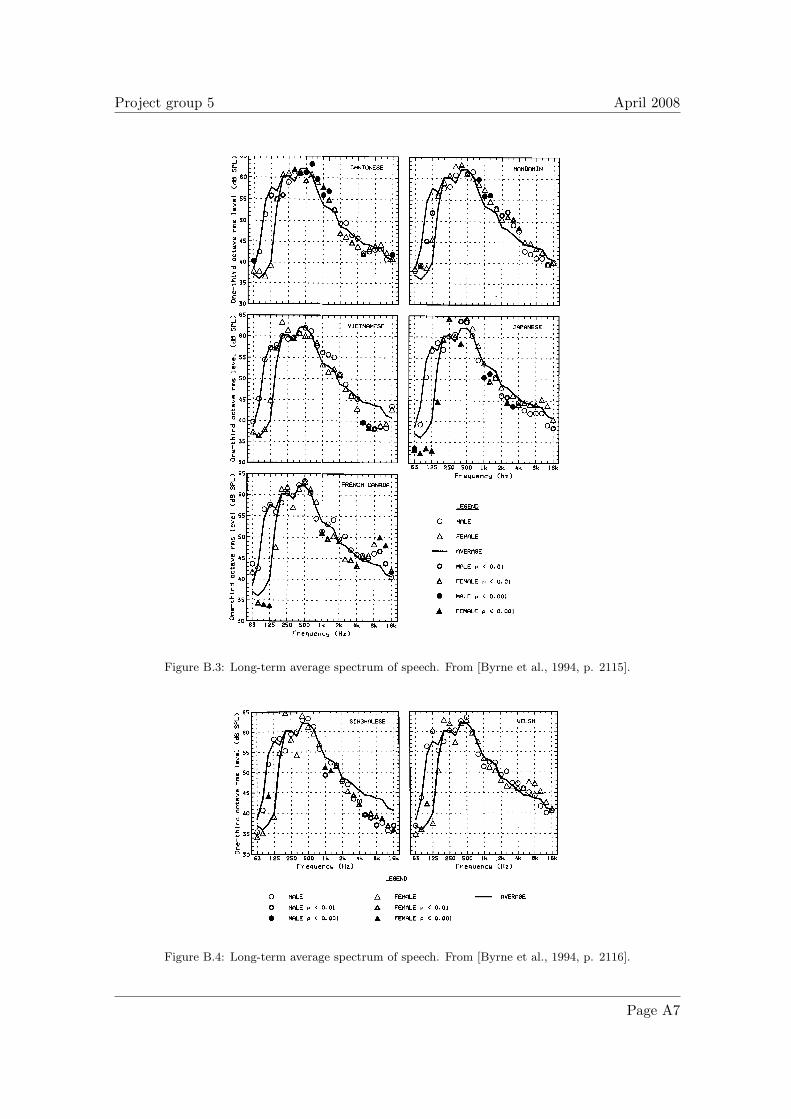
Is it very difficult though to determine the language used from a given long-term mag-nitude spectrum. This is because languages have similar long-term magnitude spectraeven though the languages are fundamentally different. This can be seen on the figuresappearing in appendix B, which show the long-term magnitude spectra for speakers ofboth genders and different languages.

There is a lot of research going on in the topic of speaker identification. Several tech-niques and strategies are used and most of them are based on the scheme shown in figure3.1.

Most of the systems use the dynamic properties of the speech signal rather than ana-lyzing the long-term spectrum. The latter requires a long signal acquisition time to betext-independent. According to figure 3.1, the different blocks can be implemented withdifferent strategies. The features extracted from the speech signal can be the cepstrumand different cepstral coefficients or the coefficients from a linear predictor (LP) based

Page 17

Chapter 3. Discussion Technical University of Denmark

’

Figure 3.1: Basic speaker identification system.

on different filter models. The length of the different speech segments is also dependingon the strategy. The output of the block after the A/D conversion is a set of vectors(describing different features of speech) that should be compared to the ones stored in adatabase, corresponding to different individuals, using the concept of distance measure-ment. Different strategies are used to determine this distance, such as pattern matchingbased on vector Euclidean distances or the use of Hidden Markov Models (HMM). Finally,a decision device has to determine the individual that provides the maximum likelihoodfor a given input signal [Campbell, 1997].


A speech shaped noise generated from a speech signal is shown in figure 2.5. The timefluctuations in the original signal (a), i.e. the envelope, disappear when the phase is ran-domized (b), while the magnitude spectrum remains unaffected by the process, (c) and (d).

In order to incorporate the fluctuations of the speech signal into the speech shaped noise,two methods are suggested, apart from the ICRA-noises generation described in section1.3. The first method, illustrated in figure 3.2, uses two inputs: random noise nI(t) anda speech signal s(t). The spectrum of the noise is equalized with the one of the speechsignal. Using the Hilbert transform, the envelope of the speech is extracted and appliedto the equalized noise. The last step is the normalization of the energy, extracted fromthe spectra of the signal and the modulated speech shaped noise.

Another method is designed to obtain speech shaped noise with modulation features usingonly a speech signal as shown in figure 3.3. Thus, the noise is obtained by making thephase of the speech random, while the magnitude spectrum is preserved. Then the enve-lope is applied and the energy is normalized in the same way as in the previous method.

The method shown in figure 3.2 has been implemented in Matlab (see Analysis_syn-



Figure 3.2: Block diagram of the used method to generate speech shaped noise with modulation features,based on the adaption of random noise to a given speech signal.

Figure 3.3: Block diagram of the used method to generate speech shaped noise with modulation features,based on the phase randomization of a given speech signal.

thesis.m function in appendix A) and it has been used to produce speech shaped noisewith speech envelope from a recorded sound file. The results are shown in figure 3.4. Itcan be seen that the amplitude of the noise (b) is higher than the amplitude of the speech(a). This is due to the fact that the fine structure of the noise is random noise and thefine structure of the speech is a periodic signal. This last signal carries the same energyas the noise with less amplitude, i.e. the speech has a lower crest factor. It can also benoted that the spectrum of the speech shaped noise is slightly different from the one ofthe speech signal (c). This is due to the convolution of the original spectrum with theenvelope spectrum, which has a reduced bandwidth as can be seen in figure 3.5.

The highest values of envelope magnitude appear at frequencies below 10 Hz, as shownin figure 3.5. It can also be seen that a secondary peak is present around 200 Hz. Thispeak represents the fundamental frequency of the speaker, in this case a female, whichhas also been observed in the long-term magnitude spectrum of the same signal in figure2.1. Therefore, it might be possible to use the envelope spectrum as a feature for speakerrecognition.

Page 19


Time [s]

0 10 20 30 40 50-0.4

-0.2

0

0.2

0.4

(a)

Time [s]

0 10 20 30 40 50-0.4

-0.2

0

0.2

0.4

(b)

Frequency [Hz]

Magnitude

[dB

]

Input noise

Speech

Output noise

102 103 104

20

25

30

35

40

45

50

55

(c)

Figure 3.4: Temporal waveforms of the speech signal (a) and the modulated speech shaped noise (b). Themagnitude spectra of both signals and the noise are used as input are shown in (c).

Envel

ope

magnit

ude

[dB

]

Modulation frequency [Hz]

1 10 100 100020

30

40

50

60

70

80

Figure 3.5: Envelope spectrum of the speech signal.



3.3 High-pass and low-pass filtered speech

In order to derive which frequency band is the most important for the intelligibility ofspeech one can convert the values of AI for the low-pass and high-pass filters, shown infigures 2.8 and 2.9, to the corresponding speech intelligibility values according to figure1.5 on page 5. The gradient of the resulting curves will be highest at the most impor-tant frequency bands for speech intelligibility. This is because, at these frequency regions,small changes in the passing bands of the filters give the highest improvements in speechintelligibility.

In figures 3.6 the dependence of AI and SII on the speech spectrum level can be seen.It can be seen that the AI increases with an increase of the speech level (figures 3.6 (a)and (b)), because the SNR increases. The slopes of the curves are rather similar amongstthem and at very low frequencies (125 Hz - 400 Hz) and very high frequencies (5 kHz -8 kHz) the values of AI, when the speech levels are “loud” and “shout” are identical. Onthe other hand, the SII presents a quite different behavior. For the low cut-off frequenciesof the high-pass filtering it can be seen that the higher the speech level the lower the SII,for cut-off frequencies up to 1.5 kHz. From that cut-off frequency and above the SII isimproving as the speech level is increasing. This behavior, which is different to the oneobserved for the AI concept, is due to the more sophisticated way that the SII procedure isimplemented. SII takes into account the different distribution of the energy in the speechspectrum at different levels and the effect of masking.

Thus, taking into consideration figure 3.6 it can be concluded that speech level affects ina different way the two indices.

3.4 Comparison of AI, SII and STI

The idea behind AI (and SII) is that background noise can influence intelligibility due tomasking and not all frequency components are equally important. STI is based on theassumption that the envelope of a speech signal must be perceived correctly in order thespeech to be understood correctly. This means that AI and SII are calculated directly fromthe magnitude response of the signals. On the other hand, the results given by STI arecorrelated with the preservation of the envelope. AI and SII are suited to estimate speechintelligibility of transmission channels in communication systems with limited bandwidth,whereas STI is calculated from the impulse response and is more suited for speech intelli-gibility in rooms.

Page 21



AI

NormalRaisedLoudShout

125 250 500 1000 2000 4000 80000

0.1

0.2

0.3

0.4

0.5

0.6

0.7

0.8

0.9

1

(a) AI - highpass


AI


125 250 500 1000 2000 4000 80000

0.1

0.2

0.3

0.4

0.5

0.6

0.7

0.8

0.9

1

(b) AI - lowpass


SII


125 250 500 1000 2000 4000 80000

0.1

0.2

0.3

0.4

0.5

0.6

0.7

0.8

0.9

1

(c) SII - highpass


SII


125 250 500 1000 2000 4000 80000

0.1

0.2

0.3

0.4

0.5

0.6

0.7

0.8

0.9

1

(d) SII - lowpass

Figure 3.6: Effect of different speech levels in the AI (a),(b) and SII (c), (d) for high-pass and low-passfiltering.



STI describes the degradation of intelligibility due to masking in the modulation domain.This correlates with the concept discussed in previous reports about the existence of amodulation filterbank that seems to play an important role in human perception. Theidea of a modulation filterbank supports the assumption that STI is based on.

Page 23

April 2008 Chapter 4. Conclusion

Chapter 4Conclusion

In this report, the intelligibility of speech has been discussed and the main conclusions arethe following:

• From the long-term magnitude spectrum, it is possible to determine the gender of thespeaker, but not the spoken language. The main peak in the spectrum correspondsto the fundamental frequency, which is around 125 Hz for male speakers and 250 Hzfor females.

• Speech-shaped noise is used as a masker for speech intelligibility tests. However, thespeech envelope is not always preserved, and some methods have been proposed togenerate speech shaped noise with the same speech envelope.

• AI and SII are affected in a different way by the change in the voice level. This isdue to the corrections on speech spectrum for different voice levels that SII applies.

• The STI is a useful parameter to assess speech intelligibility in different rooms andits calculation is based in the preservation of modulation in the speech signal. Thisseems to be in agreement with the way the auditory system perceives sounds andreinforces the assumptions of the existence of a modulation filterbank.

Page 25

Chapter 4. Conclusion Technical University of Denmark


April 2008 Bibliography

Bibliography

[Byrne et al., 1994] Byrne, D., Dillon, H., Tran, K., Arlinger, S., Wilbraham, K., Cox, R.,Hayerman, B., Hetu, R., Kei, J., Lui, C., Kiessling, J., Notby, M. N., Nasser, N. H. A.,Kholy, W. A. H. E., Nakanish, Y., Oyer, H., Powell, R., Stephens, D., Meredith, R.,Sirimanna, T., Tavartkiladze, G., Frolenkov, G. I., Westerman, S., and Ludvigsen, C.(1994). An international comparison of long-term average speech spectra. J. Acoust.Soc. Am, 96(4):2108–2120.

[Campbell, 1997] Campbell, J. (1997). Speaker recognition: A tutorial. Proceedings of theIEEE, 85(9):1437–1462.

[Dau and Christiansen, 2008] Dau, T. and Christiansen, T. U. (2008). Intelligibility ofspeech. 1.4.0 edition.

[Houtgast and Steeneken, 1973] Houtgast, T. and Steeneken, H. (1973). The modulationtransfer function in room acoustics as a predictor of speech intelligibility. Acustica,28(1):66–73.

[Houtgast and Steeneken, 1985] Houtgast, T. and Steeneken, H. (1985). The modulationtransfer function in room acoustics. B&K Technical Review, 3.

[Poulsen, 2005] Poulsen, T. (2005). Acoustic Communication, Hearing and Speech. 2.0edition. Only available from DTU campusnet.

[Poulsen, 2007] Poulsen, T. (2007). Speech. Only available from DTU campusnet.

[Steeneken and Houtgast, 1985] Steeneken, H. and Houtgast, T. (1985). Rasti: A tool forevaluating auditoria. B&K Technical Review, 3.

Page 27

Bibliography Technical University of Denmark


Project group 5 April 2008

Appendix AMatlab code

1 clc

2 clear a l l

3 close a l l

4

5 % Read wa v f i l e s

6 [y1 ,fs,Nbits]=wavread(’Speech sample 01. wav’); % Female , Eng l i sh

7 [y2 ,fs,Nbits]=wavread(’Speech sample 02. wav’); % Male , Eng l i sh

8 [y3 ,fs,Nbits]=wavread(’Speech sample 03. wav’); % Female , Danish

9 [y4 ,fs,Nbits]=wavread(’Speech sample 04. wav’); % Male , Danish

10

11 % Do something

12 N = length(y1);

13 fres=N ;%f s /N; % Reso lu t ion

14 f=fs/fres .*(0: fres /2-1); % Frequency ax i s

15

16 y1longterm =20* log10(abs( f f t (y1 ,fres)));




20

21 vLout1 = Oct3Smooth(f,y1longterm (1: fres /2),f_AI);




25

26 figure ;

27 semilogx(f,y1longterm (1: fres /2),’Color’ ,[.6 .6 .6])

28 hold on;

29 semilogx(f_AI ,vLout1 ,’k’,’LineWidth ’ ,2);

30 xlim ([100 10000])

31 ylim ([-40 70]);

32 set(gca,’XTick’ ,[100 250 500 1000 2000 4000 8000]);

33 nicefigure;

34 legend(’Long term spectrum ’,’1/3- octave smoothed spectrum ’,’Location ’,’SouthWest ’);

35 xlabel(’Frequency [Hz]’);

36 ylabel(’Magnitude [dB]’);

Page A1

APPENDIX

37 % pr i n t l a t e x ( ’ EnglishFemale ’ ,11 ,10 , ’ nof igcopy ’ ) ;

38

39 figure ;


41 hold on;


43 xlim ([100 10000])

44 ylim ([-40 70]);

45 set(gca,’XTick’ ,[100 250 500 1000 2000 4000 8000]);

46 nicefigure;




50 % pr i n t l a t e x ( ’ EnglishMale ’ ,11 ,10 , ’ nof igcopy ’ ) ;

51

52 figure ;


54 hold on;


56 xlim ([100 10000])

57 ylim ([-40 70]);

58 set(gca,’XTick’ ,[100 250 500 1000 2000 4000 8000]);

59 nicefigure;




63 % pr i n t l a t e x ( ’ DanishFemale ’ ,11 ,10 , ’ nof igcopy ’ ) ;

64

65 figure ;


67 hold on;


69 xlim ([100 10000])

70 ylim ([-40 70]);

71 set(gca,’XTick’ ,[100 250 500 1000 2000 4000 8000]);

72 nicefigure;




76 % pr i n t l a t e x ( ’ DanishMale ’ ,11 ,10 , ’ nof igcopy ’ ) ;

77

78 figure ;

79 semilogx(f_AI ,vLout1 ,’Color ’ ,[.5 .5 .5]);

80 hold on

81 semilogx(f_AI ,vLout2 ,’--’,’Color ’ ,[.5 .5 .5]);

82 semilogx(f_AI ,vLout3 ,’k’);

83 semilogx(f_AI ,vLout4 ,’--k’);

84 xlim ([100 10000])

85 ylim ([20 60]);

86 set(gca,’XTick’ ,[100 250 500 1000 2000 4000 8000]);

87 nicefigure;

88 legend(’English female ’,’English male’,’Danish female ’,’Danish male’,’Location ’,’

SouthWest ’);


Page A2 Intelligibility of Speech



91 % pr i n t l a t e x ( ’ SpecComparison ’ ,11 ,10 , ’ nof igcopy ’ ) ;

92

93 % r y1 = randomizePhase ( y1 ) ;



96 % r y4 = randomizePhase ( y4 ) ; 1 clc

2 close a l l ;

3 clear variables;

4

5 [y,fs,Nbits]=wavread(’Speech sample 01. wav’); % Female , Eng l i sh

6 N = length(y);

7 t=1/fs*(1:N);

8 f=fs/N.*(0:N/2-1); % Frequency ax i s

9 yfft= f f t (y);

10 ylongterm =20* log10(abs(yfft));

11 vLout = Oct3Smooth(f,ylongterm (1:N/2),f_AI);

12 y_energy = sum(10.^( vLout /10));

13

14 y_envelope = abs(hilbert(y));

15

16 % f i g u r e ;

17 % p l o t ( t , y , ’ Color ’ , [ . 5 .5 . 5 ] ) ;

18 % hold on

19 % p l o t ( t , y enve lope , ’ k ’ , ’ LineWidth ’ , 2 ) ;

20

21 x=rand(N,1);

22 % f i g u r e ; p l o t ( t , x , ’ Color ’ , [ . 5 .5 . 5 ] ) ;

23 % x=x .∗ y enve lope ;

24 % hold on ;

25 % p l o t ( t , x , ’ k ’ ) ;

26

27 xfft= f f t (x);

28 xlongterm =20* log10(abs(xfft));

29 xvLout = Oct3Smooth(f,xlongterm (1:N/2),f_AI);

30

31 figure (111);

32 semilogx(f_AI ,xvLout ,’--k’);

33 hold on

34

35 xfft=xfft.*abs(yfft)./abs(xfft);

36 x2longterm =20* log10(abs(xfft));

37 x2vLout = Oct3Smooth(f,x2longterm (1:N/2),f_AI);

38 semilogx(f_AI ,x2vLout ,’-k’);

39 x2= i f f t (xfft);

40

41 x2=x2.* y_envelope;

42 x2fft= f f t (x2);

43 x2longterm =20* log10(abs(x2fft));

44 x2vLout = Oct3Smooth(f,x2longterm (1:N/2),f_AI);

45 x2_energy = sum(10.^( x2vLout /10));

46 x2 = x2 * sqrt(y_energy/x2_energy);

Page A3

APPENDIX

47 figure ;

48 plot(t,x2,’k’);

49 xlabel(’Time [s]’);

50 xlim ([0 50]);

51 ylim ([-.4 .4]);

52 nicefigure;

53 printlatex(’noise2_time ’,7,8,’nofigcopy ’);

54

55

56 figure (111);

57 semilogx(f_AI ,x2vLout +10* log10(y_energy/x2_energy),’-’,’Color’ ,[.5 .5 .5]);

58 xlim ([100 10000]);


60 ylim ([20 55]);


62 nicefigure;

63 legend(’Input noise’,’Speech ’,’Output noise’,’Location ’,’SouthWest ’);

64 printlatex(’specs_mod_shape ’,9,8,’nofigcopy ’);



Appendix BLong-term average spectrum of speech

• s• ..................... I:" • •' •'"'"-" '•• '.'".. ': • • ' ' ':' ß : ' ' ' : : : : t' I'1 ...'.' •.•o.. ,, .. ..

--'i'" i--'i---::', 1 ',::::: :: , ,',','!11, ;!i ,;7!',',', ,

"'•1-'"'"'"'""'"'''"''" :,., ,,... •,•• .... .... ....,...,.._.: ,.

-"- ............... • :', O:

•"[•'1•i--•"'•---:".•'"! " "ß .... i: -,- _ .,.. _, - _ .,.

•,o [:• --•.- - ? - - -! ....... ::.-- i- ?-•,- • •'•1::'•,':- - ' :' ' ' -: ....... :"-':-".•"? -:•,•i'"!"-'i' ' ' :'":"":'".•'": ' "' • ....... ©,: I• 3• I , , I • I I • , I , • ! • • I • • I , • I • • I

• 12S 2S0 •00 lk 2k •k •k l•k

,.-, 65 . ,•-T•r1•'•r-• •. .• Frequency (Hz)

"øIi"'!, .... i"-!-"i-'-il ,-, LEGEND

'•"-o - ':---;-- -! •"•:-•'•";"':"'i o- "ør ;,o-/•---'r---i---!---i'"!- -': - •z_.-] , •,,•, • o. o, • f:v,• .., ,, . , ,, •"•"'"'""'"". ß . ß "'.... ,, ":• '•' •..' - •---i • . •. • o. oo,

63 !25 250 S00 ] ß 2k t•k 8k ]6k

Frequency

FIG. 1. Male and female long-term average speech sp:ctrum (LTASS) values for five samples of English. Solid line shows LTASS average across 17 speech samples (all samples except Arabic), males and femal :s separately for frequencies below 160 Hz, combined for higher frequencies.

no statistical examination of whether variability interacted with sample. For all samples combined, Fig. 8 shows the standard deviation of individual variations from the mean

value at each frequency for males and for females. The

analysis is based on data which had been normalized to a 70 dB overall level for each talker. The deviation values are

similar for both sexes and at all frequencies from 630 to 4000 Hz. Variability shows a small but consistent increase,

2113 J. Acoust. Soc. Am., Vol. 96, No. 4, October 1994 Byrne et aL: Long-term average speech spectra 2113

Figure B.1: Long-term average spectrum of speech. From [Byrne et al., 1994, p. 2113].

Page A5

APPENDIX

• ' •c'•) SUEDISH , •, l•li•) SUEDISH (• A• • , , STpCKHqLM , i • LINKOPINe

,,0 .... ,...,..., ...... .... ....................

•,, • ............................... •...•...•...•...?..•...•...• •30 I, , • , , • , , • , , • , , , , , • , , • , , I r• . . , , , • , , • . , • , F,. , , , . • , . •

.... .............. • ,o .•--i-•'• -'•/••' '•"":'"•'

• •o .•. •... •-..• -•• .•..-•- .y• ...................... • •'• ....... '•. J•...•..2_•.•.

•65•• Fr equenc• (Hz) • LEGEND

'•--•: 7-:---:-•L•':•-- :•--'•-•

::.. :.oo•... ;..-:• • AVERAGE

• 0 •LE • < O. O i

• •0 ...................... • FEMALE p ( O. O]

• •5 • •LE p < O. OOl

• .... •'' '• '' '%•• • FEMME p ( 0.00] 0 •0 6• ] 2S 250 •00 lk 2k 4k 8k 16k

Fr equenc• (Hz)

FIG. 2. Male and female LTASS values for Swedish (two samples), Danish, German, and Russian. Solid line shows LTASS average across 17 speech samples.

for both sexes, for bands above 4000 Hz. The only substantial increases in variability are in the bands 80 and 100 Hz for males and 125 and 160 Hz for females.

E. LTASS for Arabic

The LTASS values (dB) for Arabic, normalized to 70 dB overall level (linear), are shown in Fig. 9.

III. DISCUSSION

The overall finding of this study is that the LTASS is very similar over the wide range of languages that were ana- lyzed. Indeed, there is no single language or group of languages which could be regarded as being markedly different from the others. Therefore, it is feasible to propose a univer-

2114 J. Acoust. Soc. Am., Vol. 96, No. 4, October 1994 Byrne et aL: Long-term average speech spectra 2114




•'!'"•'T-•"•;'": .... :'";---:'• ,---•-- ,---,---•---•---,-

•,• .:.!.il..:: ...... ::...•..•...:• ; '1 •x •'"•"'•-" ;r '":' ' ' • - ": •t

030'1• • I, I Ill III I• I • • I •11i i I• • •1 I • • ' • • • • • I • • I • • I • • I • i I /

•o1: • :-••---•---:---•---• •' i ....

..... ',...;...:

• :, , , ', , ', ,, ',

•,•1-:•-•---::- ...... :• ..... •-• .... • , : : : : • , •,o1•__•___• ..... • +••

..,,,,,,,,.,,,,,,

• soE', -• ;-•-:•-;---:--- ;---;---:•

: • : : : :• ' ' ' b'" .... ',' ' ' • ' ' ':-:

......... •...•..•.

•,•[•./. J•..•...•... •...•.••..• : •o[•../...•...•... •...?...•...,:..• • •': • • : : : : : •'•F•'•---• .... , ..................... ••,, [,.[,.,,,,,,,.,,.,,

63 125 250 500 lk 2k •k 8k 16k

Frequenc•

FIG. 3. Male and female LTASS values for Canton.•se, Mandarin, Vietnamese, Japanese, and French. Solid line shows LTASS average across 17 speech samples.

sal LTASS that would be applicable to most (possibly all) languages and would be sufficiently prec se for many pur- poses. Nonetheless, there are small but (statistically) signifi- cant differences among languages and more substantial differences, at the low frequencies, between male and female talkers.

A. Male/female differences

Considering first the comparison between males and females, the most notable feature is that their spectra are vir- tually identical over the frequency range from 250 to 5000 Hz. Within this range, the normalized male and female lev-

2115 J. Acoust. Sec. Am., Vol. 96, No. 4, Octo3er 1994 Byrne et al.: Long-term average speech spectra 2115


---•65

L

,,0 L

o 3O 63 !2S 2S0 SO0 !k 2k •k $k lSk

Fr equencw (Hz)

LEOEND

MALE /• FEMALE

MALE p < 0.0! •, FEMALE p < 0.0l

MALE p < 0.001 ß FEMALE p < 0.00l

AVERROE

FIG. 4. Male and female LTASS values for Singhalese and Welsh. Solid line shows LTASS average across 17 speech samples.

TABLE II. Male, Female, and combined speech spectra, normalized for 70 dB SPL overall level and averaged across samples (excluding Arabic). Com- bined is equal to male for frequencies up to 160 Hz; it is average of male and females for other frequencies. The spectrum (combined male and female) recommended by Cox and Moore (1988) is also shown.

Frequency Cox and Moore (Hz) Male Female Combined (1988)

63 38.6 37.0 38.6 ...

80 43.5 36.0 43.5 --.

100 54.4 37.5 54.4 ...

125 57.7 40.1 57.7 ...

160 56.8 53.4 56.8 ...

200 58.2 62.2 60.2 '" 250 59.7 60.9 60.3 60.0

315 60.0 58.1 59.0 57.0 400 62.4 61.7 62.1 61.0 500 62.6 61.7 62.1 62.0

630 60.6 60.4 60.5 59.0 800 55.7 58.0 56.8 56.5

1000 53.1 54.3 53.7 55.0

1250 53.7 52.3 53.0 54.5 1600 52.3 51.7 52.0 52.0 2000 48.7 48.8 48.7 49.0

2500 48.9 47.3 48.1 48.0 3150 47.0 46.7 46.8 46.5 4000 46.0 45.3 45.6 46.0

5000 44.4 44.6 44.5 44.0 6300 43.3 45.2 44.3 45.5 8000 42.4 44.9 43.7 "'

10 000 41.9 45.0 43.4 ."

12 500 39.8 42.8 41.3 ... 16 000 40.4 41.1 40.7 ...

els, averaged over all languages, agree within 2 dB at all third-octave frequencies except 800 Hz, where the difference is 2.3 dB. (The non-normalized values agree almost as closely as there was little difference between the average overall male and female speech levels.) For frequencies of 160 Hz and below, male levels greatly exceeded female levels undoubtably because of the difference in the fundamental frequency ranges. These findings are consistent across languages and consistent with previous research (Benson and Hirsh, 1953; Tarnoczy and Fant, 1964; Tarnoczy, 1971; Ni- emoller et al., 1974; Byrne, 1977; Pearsons et al., 1977; Cox and Moore, 1988).

140

120

100 80 6O

40

2O

0

54 58 62 66 70 74 78 82 86

Long term rms level (rib $PL)

FIG. 5. Distribution of overall rms levels (measured at 20 cm from mouth). Curve shows normal distribution fitted to data.

2116 J. Acoust. Soc. Am., Vol. 96, No. 4, October 1994 Byrne et al.: Long-term average speech spectra 2116


Page A7

intelligibility of speech - troels...

Documents