inter-sectoral labor immobility, sectoral co-movement, and

Kyoto University, Graduate School of Economics Discussion Paper Series

Inter-sectoral Labor Immobility, Sectoral Co-movement, and News Shocks

Munechika Katayama and Kwang Hwan Kim

Discussion Paper No. E-15-011

Graduate School of Economics Kyoto University

Yoshida-Hommachi, Sakyo-ku Kyoto City, 606-8501, Japan

December, 2015

Inter-sectoral Labor Immobility, Sectoral Co-movement, and

News Shocks⇤

Munechika Katayama

Kyoto University

[email protected]

Kwang Hwan Kim

Yonsei University

[email protected]

December 2015

Abstract

The sectoral co-movement of output and hours worked is a prominent feature of business

cycle data. However, most two-sector neoclassical models fail to generate this sectoral co-

movement. We construct and estimate a two-sector neoclassical DSGE model that generates

the sectoral co-movement in response to both anticipated and unanticipated shocks. The key to

our model’s success is a significant degree of inter-sectoral labor immobility, which we estimate

using data on sectoral hours worked. Furthermore, we demonstrate that imperfect inter-sectoral

labor mobility provides a better explanation for the sectoral co-movement than some alternative

model emphasizing the role of labor-supply wealth e↵ects.

Keywords: Sectoral Co-movement; Labor Immobility; Non-separable Preferences; Unantici-

pated Shocks; News Shocks.

JEL Classification: E32; E13

⇤We would like to thank the following for their valuable comments and suggestions: Pablo Guerron-Quintana, JinillKim, Ryo Jinnai, Toshiaki Watanabe, seminar and conference participants at Yonsei University, the Bank of Japan, KyotoUniversity, Australian National University, Tohoku University, the 2011 Midwest Macroeconomics Meetings, the 2011Asian Meetings of the Econometric Society, the 2011 annual meetings of the Southern Economic Association, 2012 SpringMeeting of the Japanese Economic Association, and the International Conference “Frontiers in Macroeconometrics” atHitotsubashi University. This paper was previously circulated as “Costly Labor Reallocation, Non-Separable Preferences,and Expectation Driven Business Cycles.” A part of this study was financially supported by JSPS Grants-in-Aid forScientific Research 15K17020.

1

1 Introduction

Sectoral co-movement is an important characteristic of business cycles. Output, hours worked,

and investment tend to co-move across sectors over business cycles. Synchronization of sectoral

variables leads to the co-movement of aggregate macroeconomic variables, and it is crucial for

business cycle models to generate sectoral co-movement.

However, standard neoclassical business cycle models fail to generate sectoral co-movement

in response to contemporaneous (unanticipated) shocks. For example, Christiano and Fitzgerald

(1998) show that the two-sector neoclassical model driven by aggregate contemporaneous total

factor productivity (TFP) shocks cannot generate sectoral co-movement of hours worked across

industries that produce consumption and investment goods. Greenwood et al. (2000) show that

co-movement between the consumption and investment sectors is also di�cult to generate in the

two-sector model with contemporaneous investment-specific technology shocks.

Recently, there has been a resurgent interest in understanding the source of sectoral co-

movement. This has been stimulated by a revival of interest in the idea that changes in expectations

about future fundamentals, (i.e., news shocks or anticipated shocks) might be important drivers

of economic fluctuations. News shocks pose an additional challenge to business cycle models in

generating sectoral co-movement. As Beaudry and Portier (2004) and Jaimovich and Rebelo (2009)

demonstrate, it is di�cult for news shocks to generate the co-movement in output, hours worked,

and investment across sectors of the economy.

In this study, we construct and estimate a two-sector neoclassical business cycle model that can

generate sectoral co-movement in response to both contemporaneous and news shocks.1 We restrict

our attention to a neoclassical environment in order to better understand the nature of sectoral

co-movement with respect to contemporaneous and news shocks and to maintain comparability

with earlier studies, such as those by Christiano and Fitzgerald (1998), Greenwood et al. (2000), and

Jaimovich and Rebelo (2009).1There is a strand of literature on news shocks that has examined the co-movement of aggregate macroeconomic

variables in one-sector business cycle models. Several recent papers have proposed a one-sector model that produces theaggregate co-movement. Examples include Christiano, Ilut, Motto, and Rostagno (2008), Den Haan and Kaltenbrunner(2009), Dupor and Mehkari (2014), Eusepi and Preston (2009), Gunn and Johri (2011), Guo et al. (2015), Karnizova (2010),Pavlov and Weder (2013), and Wang (2012). However, we focus on the sectoral co-movement problem because aggregateco-movement does not necessarily imply sectoral co-movement in a two-sector setup. In contrast, once we generatesectoral co-movement, aggregate co-movement naturally follows.

2

In our model, imperfect inter-sectoral labor mobility and non-separable preferences between

consumption and leisure are key to generating sectoral co-movement. To show their importance,

we analytically illustrate a condition for sectoral co-movement. In fact, our co-movement condi-

tion is based on equilibrium conditions. Thus, our mechanism not only works for responses to

anticipated shocks, but also applies to contemporaneous shocks.2 We then estimate key model

parameters related to sectoral co-movement using Bayesian techniques. The data support our pro-

posed mechanism of generating sectoral co-movement. In particular, we find that imperfect labor

mobility across sectors plays a crucial role in sectoral co-movement. Although the estimated degree

of non-separability is moderate, non-separable preferences help generate the co-movement.

There is abundant empirical evidence supporting the main feature of our model, inflexible inter-

sectoral labor mobility. Davis and Haltiwanger (2001) find limited labor mobility across sectors in

response to monetary and oil shocks. Horvath (2000) reports a relatively low estimate for the

elasticity of substitution of labor across sectors, using sectoral U.S. labor hours data. Beaudry and

Portier (2011) present evidence of labor market segmentation through various panel estimations

based on PSID data. In particular, their results suggest that the mobility across sectors is not

su�cient to equate the returns to labor between individuals initially attached to di↵erent sectors.

This evidence is probably the closest to the spirit of the model considered in this paper. Non-

separable preferences also play an important role in the transmission of monetary policy shocks in

New Keynesian models (e.g., Guerron-Quintana, 2008; Kim and Katayama, 2013).

Another important contribution of this study is that our approach to generating sectoral co-

movement in response to contemporaneous and news shocks is more consistent with the data than

an alternative mechanism is. In particular, our study is closely related to a two-sector version of the

model by Jaimovich and Rebelo (2009), which is considered a leading mechanism for generating

sectoral co-movement in the literature. In their model, a very weak wealth e↵ect on the labor

supply is a source of sectoral co-movement. To show this, they introduce a new class of preferences,

featuring a parameter that governs the strength of the wealth e↵ect of labor supply. To compare

the empirical performance of our model with theirs, we also estimate their two-sector model. We

show that our model outperforms theirs in terms of the Bayes factor and matching business cycle2In this study, we use the terms contemporaneous shocks and unanticipated shocks interchangeably. Similarly, we use

news shocks and anticipated shocks interchangeably.

3

moments.

Why does the data support our model over that of Jaimovich and Rebelo (2009)? We find

that the estimated degree of the labor supply wealth e↵ect is very close to zero in their two-sector

model, so in principle, the model could deliver sectoral co-movement. Our estimate of the labor

supply wealth e↵ect is consistent with the results of Schmitt-Grohe and Uribe (2012), who estimate

the one-sector version of Jaimovich and Rebelo (2009). However, the estimated two-sector version

of the Jaimovich and Rebelo (2009) model does not generate the observed positive correlations of

output and hours worked across sectors even with the near-zero wealth e↵ect, and thus, the data

favor our model over theirs. We demonstrate that the ability of the Jaimovich and Rebelo (2009)

model to generate sectoral co-movement is in turn related to the marginal cost of varying capital

utilization, which is also crucial in their model. To support sectoral co-movement, the cost must be

small; however, this cost is estimated to be too high in the consumption sector, which prevents their

two-sector model from generating sectoral co-movement.

Although we restrict ourselves to a neoclassical environment, our finding has an implication

for sectoral co-movement in a New Keynesian setup.3 Khan and Tsoukalas (2012) estimate a one-

sector New Keynesian model featuring Jaimovich–Rebelo preferences. Unlike Schmitt-Grohe and

Uribe (2012), they find that the estimated size of the labor supply wealth e↵ect is non-negligible in a

one-sector New Keynesian setup. The findings in Khan and Tsoukalas (2012) and our study suggest

that it may be di�cult to rely on Jaimovich–Rebelo preferences to generate sectoral co-movement

in a two-sector New Keynesian model, and imperfect labor mobility across sectors may be a useful

device for this purpose.

There are several other studies on generating the sectoral co-movement to news shocks in multi-

sector neoclassical business cycle models as well.4 For example, Beaudry and Portier (2004) show

that strong complementarity between non-durable and durable goods in the momentary utility

function can overcome the sectoral co-movement problem. Beaudry and Portier (2007) identify the

cost complementarity among intermediate goods firms in a multi-sector setting (i.e., economies of

scope) as a key feature that generates co-movement. Beaudry et al. (2011) analyze a two-country3For example, Davis (2007), Fujiwara et al. (2011), and Khan and Tsoukalas (2012) use one-sector New Keynesian

models to assess the quantitative importance of news shocks.4See Beaudry and Portier (2013) for an exhaustive list of studies that may generate the sectoral co-movement in

response to news shocks.

4

two-sector model and discuss conditions for business cycle fluctuations driven by news shocks.

Although these mechanisms are interesting possible mechanisms of producing the sectoral co-

movement, prior studies explore only theoretical perspectives.5 Our study is di↵erent in that we

not only propose a potential explanation for the co-movement problem, but also show that it is

supported by the data.

We also evaluate the importance of news shocks in accounting for business cycle fluctuations.

Although existing studies typically use one-sector DSGE models to empirically evaluate the impor-

tance of news shocks, we tackle the same question through the lens of our two-sector model. As

in Khan and Tsoukalas (2012) and Schmitt-Grohe and Uribe (2012), we find that the news compo-

nents of wage markup shocks play an important role in explaining business cycle fluctuations. In

particular, variations in hours growth are largely attributed to news components in wage markup

shocks. Even though technology news shocks typically play negligible roles in Khan and Tsoukalas

(2012) and Schmitt-Grohe and Uribe (2012),6 we find that they are non-negligible. In fact, our

results are quantitatively similar to the findings in Fujiwara et al. (2011). However, the overall

contribution of technology news shocks is not so significant, relative to unanticipated counterparts

(contemporaneous technology shocks).

The remainder of the paper is organized as follows. Section 2 presents our two-sector neoclassi-

cal DSGE model. Section 3 characterizes the necessary condition for sectoral co-movement in hours

worked analytically, and provides numerical simulations to illustrate our model. Section 4 presents

the Bayesian estimation of the structural parameters of our model. Section 5 compares the empirical

performance of our model with that of a two-sector version of the model proposed by Jaimovich

and Rebelo (2009). Finally, Section 6 concludes the paper.5For example, existing empirical studies seem to suggest that the consumption of non-durable and of durable goods are

generally not complements. For instance, Ogaki and Reinhart (1998) estimate the intratemporal elasticity of substitutionbetween non-durable and durable goods consumption. They find that this elasticity is greater than one, implying that non-durable goods and consumer durable goods are substitutes. Piazzesi, Schneider, and Tuzel (2007) find that non-durablesand housing are substitutes.

6The exception is anticipated components in stationary investment-specific technology shocks in Schmitt-Grohe andUribe (2012) for investment growth.

5

2 The Model

Our model adopts the basic structure of the two-sector model of Jaimovich and Rebelo (2009), but

di↵ers from their model in two respects. Jaimovich and Rebelo (2009) use a new class of preferences

parameterizing the strength of wealth e↵ects on the labor supply. These preferences nest the class

of the utility functions proposed by King et al. (1988) (i.e., KPR preferences) and by Greenwood,

Hercowitz, and Hu↵man (1988) (i.e., GHH preferences), which eliminates the wealth e↵ects on the

labor supply, as special cases. In contrast, we restrict our focus to the standard King–Plosser–Rebelo

utility function to show that our model is capable of generating the business cycle sectoral co-

movement without assuming very low wealth e↵ects on the labor supply. In addition, we assume

that labor is not perfectly mobile across sectors and thus wages are not equalized across the sectors,

in contrast to Jaimovich and Rebelo (2009).

2.1 Households

The economy is populated by a constant number of identical and infinitely lived households. The

representative household receives utility from consumption and incurs disutility from providing

labor hours to the consumption and investment goods sectors. Let C

t

and N

t

denote the consumption

in period t and an aggregate labor index, respectively. Households maximize their expected lifetime

utility, given by

U0 = E0

26666641X

t=0

�t

b

t

U(Ct

� hC

t�1,Nt

)

3777775 , (1)

where � 2 (0, 1) is the subjective discount factor and h 2 [0, 1) governs the degree of internal habit

formation. The variable b

t

denotes an exogenous and stochastic preference shock in period t. This

type of disturbance has been found to be an important source of consumption fluctuations in most

existing econometric estimations of DSGE macroeconomic models (e.g., Smets and Wouters, 2007;

Justiniano et al., 2010).

In this study, we use the following specific form of the King–Plosser–Rebelo utility function:

U(Ct

� hC

t�1,Nt

) =(C

t

� hC

t�1)1� 1�

⇣1 +

⇣1� � 1

⌘v(N

t

)⌘ 1� � 1

1 � 1�

, � 1, (2)

6

where v(Nt

) = ' ⌘1+⌘N

t

⌘+1⌘ . This class of the King–Plosser–Rebelo utility function is also used in Basu

and Kimball (2002), Shimer (2009), Kim and Katayama (2013), and Katayama and Kim (2013). The

term v(Nt

) measures the disutility incurred from hours worked, with v

0> 0, v

00 > 0. The parameter

⌘ is the Frisch elasticity of aggregate labor supply in the absence of habit formation (i.e., h = 0),

measuring the intertemporal elasticity of aggregate labor supply.7 For lower values of ⌘, agents are

unwilling to substitute aggregate labor supply over time.

Our formulation of the momentary utility function nests the non-separable and separable

preferences in consumption and leisure. In (2), the degree of non-separability is controlled by the

parameter for intertemporal elasticity of substitution for consumption, �. The non-separable cases

arise when � < 1, which implies that consumption and leisure are substitutes, as predicted by theory

of time allocation (Becker, 1965). In other words, the marginal utility of consumption is decreasing

in leisure. Lower values for this parameter imply a larger substitutability between consumption

and leisure displayed by the utility function. The separable case corresponds to the limiting case

�! 1,

lim�!1

U(Ct

� hC

t�1,Nt

) = log(Ct

� hC

t�1) � v(Nt

).

This separable preference is used in most business cycle models.

We assume that the representative household is endowed with one unit of time in each period,

and that the aggregate leisure index, L

t

, takes the following form:

L

t

= 1 �N

t

= 1 �N

✓+1✓

c,t +N

✓+1✓

i,t

� ✓✓+1, ✓ � 0. (3)

Here N

t

is an aggregate labor hours index, and N

c,t and N

i,t denote labor hours devoted to the

consumption and the investment sector, respectively. This specification is considered by Hu↵man

and Wynne (1999) and Horvath (2000) to capture some degree of sector specificity to labor without

deviating from the representative worker assumption. The degree to which labor can move across

sectors is controlled by the elasticity of intratemporal substitution in labor supply, ✓. As ✓ ! 1,7It can be easily shown that the inverse Frisch elasticity of labor supply (i.e., the marginal utility of consumption (�)

constant elasticity) is @logW

@logN

!

�=const.

=hU

NN

� (UCN

)2/UCC

i/U

N

,

where � is the marginal utility of consumption and W is the real wage. After some algebra, one can show that the inverseFrisch elasticity reduces to 1/⌘.

7

labor hours become perfect substitutes for the worker, implying that the worker would devote all

time to the sector paying the highest wage. Hence, at the margin, all sectors pay the same hourly

wage. For ✓ < 1, hours worked are not perfect substitutes for the worker. The worker has a

preference for diversity of labor, and hence would prefer working positive hours in each sector,

even when the wages are di↵erent among sectors. As ✓ ! 0, it becomes impossible to alter the

composition of labor hours. In other words, there is an infinite cost of doing so and, consequently,

the labor hours in two di↵erent sectors will be perfectly correlated. Below, we will derive the

threshold level of ✓ needed to produce the sectoral co-movement of hours worked.

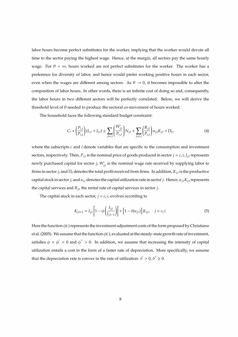
The household faces the following standard budget constraint:

C

t

+

P

i,t

P

c,t

!(I

c,t + I

i,t) X

j=c,i

0BBBB@

W

⇤j,t

P

c,t

1CCCCA N

j,t +X

j=c,i

R

j,t

P

c,t

!u

j,tKj,t +⇧t

, (4)

where the subscripts c and i denote variables that are specific to the consumption and investment

sectors, respectively. Then, P

j,t is the nominal price of goods produced in sector j = c, i, I

j,t represents

newly purchased capital for sector j, W

⇤j,t is the nominal wage rate received by supplying labor to

firms in sector j, and⇧t

denotes the total profit received from firms. In addition, K

j,t is the productive

capital stock in sector j, and u

j,t denotes the capital utilization rate in sector j. Hence, u

j,tKj,t represents

the capital services and R

j,t the rental rate of capital services in sector j.

The capital stock in each sector, j = c, i, evolves according to

K

j,t+1 = I

j,t

"1 � �

I

j,t

I

j,t�1

!#+

h1 � �(u

j,t)i

K

j,t, j = c, i. (5)

Here the function�(·) represents the investment adjustment costs of the form proposed by Christiano

et al. (2005). We assume that the function�(·), evaluated at the steady-state growth rate of investment,

satisfies � = �0 = 0 and �00> 0. In addition, we assume that increasing the intensity of capital

utilization entails a cost in the form of a faster rate of depreciation. More specifically, we assume

that the depreciation rate is convex in the rate of utilization: �0 > 0, �00 � 0.

8

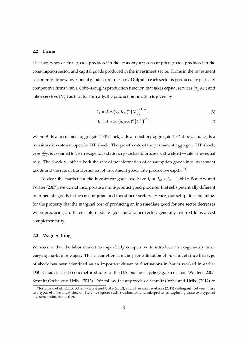
2.2 Firms

The two types of final goods produced in the economy are consumption goods produced in the

consumption sector, and capital goods produced in the investment sector. Firms in the investment

sector provide new investment goods to both sectors. Output in each sector is produced by perfectly

competitive firms with a Cobb–Douglas production function that takes capital services (uj,tKj,t) and

labor services (Nd

j,t) as inputs. Formally, the production function is given by

C

t

= A

t

a

t

�u

c,tKc,t�↵ ⇣

N

d

c,t

⌘1�↵, (6)

I

t

= A

t

a

t

z

i,t�u

i,tKi,t�↵ ⇣

N

d

i,t

⌘1�↵, (7)

where A

t

is a permanent aggregate TFP shock, a

t

is a transitory aggregate TFP shock, and z

i,t is a

transitory investment-specific TFP shock. The growth rate of the permanent aggregate TFP shock,

g

t

⌘ A

t

A

t�1, is assumed to be an exogenous stationary stochastic process with a steady-state value equal

to g. The shock z

i,t a↵ects both the rate of transformation of consumption goods into investment

goods and the rate of transformation of investment goods into productive capital. 8

To clear the market for the investment good, we have I

t

= I

c,t + I

i,t. Unlike Beaudry and

Portier (2007), we do not incorporate a multi-product good producer that sells potentially di↵erent

intermediate goods to the consumption and investment sectors. Hence, our setup does not allow

for the property that the marginal cost of producing an intermediate good for one sector decreases

when producing a di↵erent intermediate good for another sector, generally referred to as a cost

complementarity.

2.3 Wage Setting

We assume that the labor market as imperfectly competitive to introduce an exogenously time-

varying markup in wages. This assumption is mainly for estimation of our model since this type

of shock has been identified as an important driver of fluctuations in hours worked in earlier

DSGE model-based econometric studies of the U.S. business cycle (e.g., Smets and Wouters, 2007;

Schmitt-Grohe and Uribe, 2012). We follow the approach of Schmitt-Grohe and Uribe (2012) to8Justiniano et al. (2011), Schmitt-Grohe and Uribe (2012), and Khan and Tsoukalas (2012) distinguish between these

two types of investment shocks. Here, we ignore such a distinction and interpret z

i,t as capturing these two types ofinvestment shocks together.

9

our two-sector economy in modeling the labor market. We assume that there are continua of

monopolistically competitive type-specific labor unions in each sector, j, selling di↵erentiated labor

services to firms.

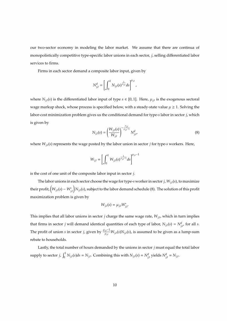
Firms in each sector demand a composite labor input, given by

N

d

j,t =

"Z 1

0N

j,t(s)1µ

j,tds

#µj,t

,

where N

j,t(s) is the di↵erentiated labor input of type s 2 [0, 1]. Here, µj,t is the exogenous sectoral

wage markup shock, whose process is specified below, with a steady-state value µ � 1. Solving the

labor-cost minimization problem gives us the conditional demand for type-s labor in sector j, which

is given by

N

j,t(s) =

W

j,t(s)W

j,t

!� µj,t

µj,t�1

N

d

j,t, (8)

where W

j,t(s) represents the wage posted by the labor union in sector j for type-s workers. Here,

W

j,t =

"Z 1

0W

j,t(s)1

µj,t�1

ds

#µj,t�1

is the cost of one unit of the composite labor input in sector j.

The labor unions in each sector choose the wage for type-s worker in sector j, W

j,t(s), to maximize

their profit,✓W

j,t(s) �W

⇤j,t

◆N

j,t(s), subject to the labor demand schedule (8). The solution of this profit

maximization problem is given by

W

j,t(s) = µj,tW

⇤j,t.

This implies that all labor unions in sector j charge the same wage rate, W

j,t, which in turn implies

that firms in sector j will demand identical quantities of each type of labor, N

j,t(s) = N

d

j,t, for all s.

The profit of union s in sector j, given by µ j,t�1µ

j,tW

j,t(s)Nj,t(s), is assumed to be given as a lump-sum

rebate to households.

Lastly, the total number of hours demanded by the unions in sector j must equal the total labor

supply to sector j,R 1

0 N

j,t(s)ds = N

j,t. Combining this with N

j,t(s) = N

d

j,t yields N

d

j,t = N

j,t.

10

3 Inspecting the Mechanism

Before we take our model to the data, we study the key mechanism generating the co-movement

analytically, and then numerically investigate our model. To this end, it is useful to focus on the

special case in which there is no habit formation in the preferences and the labor market is perfectly

competitive (i.e., h = 0 and µj,t = 1).

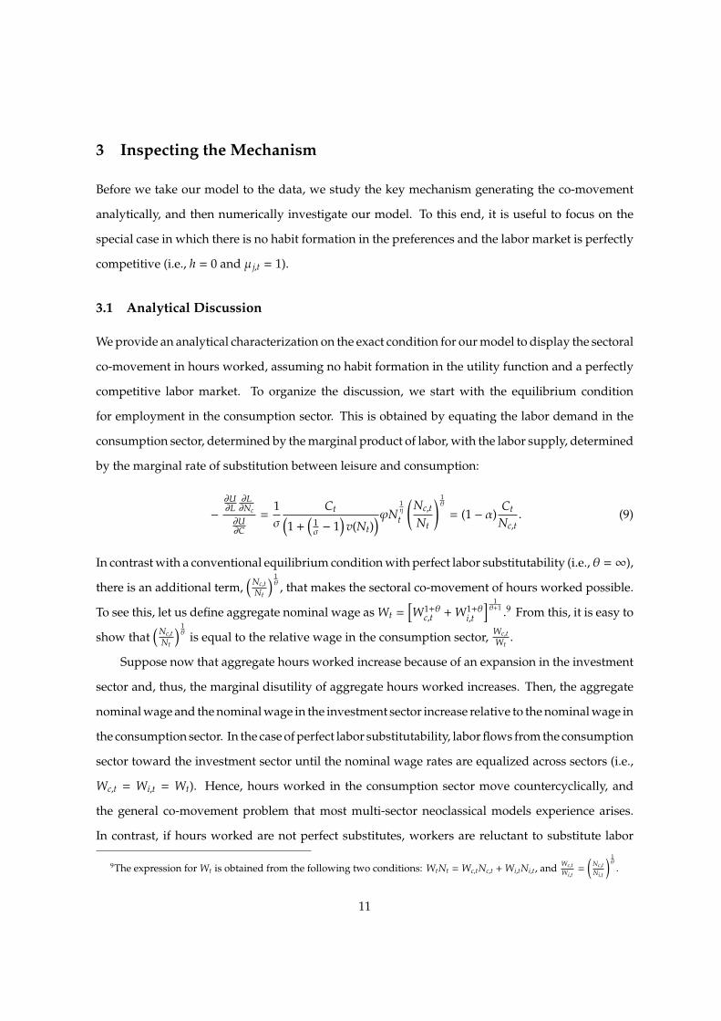
3.1 Analytical Discussion

We provide an analytical characterization on the exact condition for our model to display the sectoral

co-movement in hours worked, assuming no habit formation in the utility function and a perfectly

competitive labor market. To organize the discussion, we start with the equilibrium condition

for employment in the consumption sector. This is obtained by equating the labor demand in the

consumption sector, determined by the marginal product of labor, with the labor supply, determined

by the marginal rate of substitution between leisure and consumption:

�@U

@L

@L

@N

c

@U

@C

=1�

C

t⇣1 +

⇣1� � 1

⌘v(N

t

)⌘'N

1⌘

t

N

c,t

N

t

! 1✓

= (1 � ↵)C

t

N

c,t. (9)

In contrast with a conventional equilibrium condition with perfect labor substitutability (i.e., ✓ = 1),

there is an additional term,⇣

N

c,tN

t

⌘ 1✓ , that makes the sectoral co-movement of hours worked possible.

To see this, let us define aggregate nominal wage as W

t

=hW

1+✓c,t +W

1+✓i,t

i 1✓+1 .9 From this, it is easy to

show that⇣

N

c,tN

t

⌘ 1✓ is equal to the relative wage in the consumption sector, W

c,tW

t

.

Suppose now that aggregate hours worked increase because of an expansion in the investment

sector and, thus, the marginal disutility of aggregate hours worked increases. Then, the aggregate

nominal wage and the nominal wage in the investment sector increase relative to the nominal wage in

the consumption sector. In the case of perfect labor substitutability, labor flows from the consumption

sector toward the investment sector until the nominal wage rates are equalized across sectors (i.e.,

W

c,t = W

i,t = W

t

). Hence, hours worked in the consumption sector move countercyclically, and

the general co-movement problem that most multi-sector neoclassical models experience arises.

In contrast, if hours worked are not perfect substitutes, workers are reluctant to substitute labor

9The expression for W

t

is obtained from the following two conditions: W

t

N

t

=W

c,tNc,t +W

i,tNi,t, and W

c,tW

i,t=

✓N

c,tN

i,t

◆ 1✓

.

11

across sectors. Thus, nominal wage rates will not be equalized across sectors, and the relative

wage in the consumption sector will remain low. This low relative wage in the consumption sector

makes consumption-good producing firms demand more labor, which mitigates the co-movement

problem.

To derive the condition for the sectoral labor co-movement, we log-linearize (9) around a steady

state10 and obtain✓1 +

1✓

◆N

c,t =

1✓+ !

N

� 1⌘

!N

t

, (10)

where !N

⌘ ( 1��1)v

0 (N)N(1+( 1

��1)v(N)) and lim�!1!N

= 0. We can show that !N

= (1 � �)⇣

N

N

c

⌘ 1✓+1

W

c

N

c

P

c

C

� 0, for

� 1. Note that (10) holds for all t.

Therefore, our model displays sectoral labor co-movement if the following condition holds:

1✓+ !

N

� 1⌘> 0. (11)

Our mechanism does not need to rely on preferences exhibiting no wealth e↵ects on the labor supply

or intermediate goods sectors exhibiting cost complementarity.

In contrast, it is easy to see that this condition does not hold when preferences are additively

separable and labor is perfectly mobile (i.e., !N

! 0 and ✓!1), which most neoclassical business

cycle models assume. As discussed above, in this case, labor hours in the consumption sector move

in the opposite direction of aggregate hours. Again, this is the general co-movement problem that

has drawn a lot of attention in the literature. Condition (11) has some interesting implications that

deserve further comment.

First, notice that (11) is obtained using a temporal equilibrium condition. In other words, we

derive it using the current market clearing condition for labor. Hence, (11) guarantees a sectoral co-

movement of labor in response to a change in expectation about future fundamentals, irrespective of

whether it is correctly forecasted or whether it is based on false perceptions. Furthermore, since (11)

does not depend on the nature of shocks, it is not specific to the case of the anticipated shocks. There-

fore, (11) also ensures sectoral co-movement in response to an unanticipated aggregate TFP shock,

investment-sector TFP shock, and a preference shock. While we assume a perfectly competitive10In so doing, we implicitly assume that the growth rate of a permanent aggregate TFP shock, (g), is 1.

12

labor market (i.e., µj,t = 1, for all t) in this analytical discussion, it is easy to show that introducing

an imperfect competitive labor market does not change the aforementioned characteristics of the

sectoral labor condition, (11). In the case of an imperfectly competitive labor market (i.e., µj,t > 1),

the equation analogous to (10) is

✓1 +

1✓

◆N

c,t =

1✓+ !

N

� 1⌘

!N

t

� µc,t,

where !N

= (1 � �)⇣

N

N

c

⌘ 1✓+1

W

c

N

c

P

c

C

1µ

c

. Note that !N

is slightly di↵erent to !N

owing to the imperfect

competition in the labor market. Apparent from this equation, our model predicts the sectoral labor

co-movement of labor in response to any kind of the anticipated and unanticipated shocks, with the

exception of a contemporaneous consumption-sector wage markup shock, as long as condition (11)

is satisfied.

Second, the non-separability in itself is not su�cient to generate the sectoral employment co-

movement with perfect labor mobility. The reason is that the condition for the model to generate the

co-movement when there is perfect labor mobility violates the normality of consumption and leisure.

When building models with non-separable preferences to analyze business cycle fluctuations, Bilbiie

(2009) emphasizes that one needs to check the conditions for overall concavity of the momentary

utility function and the normality of consumption and leisure. It is straightforward to show that if

� 1, the overall concavity of U(·) is guaranteed (i.e., U

CC

0, U

LL

0 and U

CC

U

LL

� (UCL

)2 � 0).

To ensure that consumption and leisure are normal goods, the constant-consumption labor supply

needs to be upward sloping.11 In other words, the following restriction to U(·) needs to hold:

� N

U

LL

U

L

�N

U

CL

U

C

!= �!

N

+1⌘> 0. (12)

11More precisely, Bilbiie (2009) shows that both consumption and leisure are normal goods if

(UCL

/UL

) � (UCC

/UC

)(U

LL

/UL

) � (UCL

/UC

)< 0.

It is straightforward to show that the numerator is always positive in our momentary utility function. Hence, to ensurethe normality of consumption and leisure, the denominator, the constant-consumption labor supply, should be positive.

13

However, when ✓!1, (11) reduces to

�!N

+1⌘< 0.

This condition contradicts the normality condition of consumption and leisure, given in (12). Thus,

non-separability per se cannot guarantee sectoral co-movement.

Third, even though non-separability alone cannot guarantee the co-movement, it expands

the threshold level of the intratemporal elasticity of labor supply, ✓, needed to generate sectoral

employment co-movement.

Fourth, when the intertemporal elasticity of aggregate labor supply (the Frisch elasticity) is equal

to the intratemporal elasticity of labor supply (i.e., ⌘ = ✓), v(Nt

) takes the form v(Nt

) = N

✓+1✓

c,t +N

✓+1✓

i,t .

This e↵ectively isolates each sector’s labor supply pool, which insulates sectors from rising costs in

other areas of the economy. In this case, it is essential to have the non-separability in consumption

and labor supply for the model to generate the co-movement. The economic intuition is simple:

The non-separability in consumption and leisure implies that consumption and aggregate labor are

complements. Therefore, it is likely that hours worked in the consumption sector move together

with aggregate hours worked.

Finally, note that while (11) would produce the sectoral employment co-movement, it is silent

about whether it would generate economic fluctuations observed in business cycle data in response

to anticipated shocks. If aggregate labor decreases in response to a positive anticipated TFP shock

because of wealth e↵ects, for example, then (11) would imply a drop in employment in both the

consumption and investment sectors. In the next subsection, we demonstrate numerically that the

size of the investment adjustment costs determine whether aggregate labor and investment increase

on receipt of a positive news shock, so that (11) generates an increase in labor in both sectors.

3.2 Anatomy of the Model

We numerically illustrate responses of our model to di↵erent types of shocks to obtain more insight

into the underlying mechanism. In particular, we show how (i) frictions in labor mobility, (ii) non-

separable preferences, (iii) investment adjustment costs, and (iv) variable capital utilization play

a role in generating sectoral co-movement. Even though we have introduced more shocks in our

14

model for estimation purposes, we focus on the dynamic responses of macroeconomic variables to

aggregate TFP and investment-specific technology shocks, which are also analyzed in Jaimovich

and Rebelo (2009).

The parameter values used for the numerical simulations are as follows. To be comparable,

we use the same values for the following parameters as Jaimovich and Rebelo (2009). We set

the discount factor (�) to 0.985 and the capital share (↵) to 0.36. We assume that the steady-state

depreciation rate is the same across sectors, and set it to 0.025. We choose the second derivative

of the investment-adjustment costs function evaluated at the steady state, �00 , to equal 1.3. The

elasticity of �0(·), evaluated in the steady state ( ⌘ �00(uj

)uj

/�0(u

j

), where u

j

is the level of utilization

in sector j = c, i in the steady state) is assumed to be the same across sectors and is set to 0.15.

Following Basu and Kimball (2002), we set the intertemporal elasticity of substitution in con-

sumption (�) to 0.5, which implies that consumption and labor are complements in the utility

function. The parameter ✓, which determines the elasticity of substitution between hours worked

in di↵erent sectors, is set to one, based on the empirical work by Horvath (2000).12 We set the Frisch

elasticity of aggregate labor supply (⌘) to 1.13 The consumption share in the steady state ( C

C+pI

) is set

to 0.78, consistent with the U.S. data.

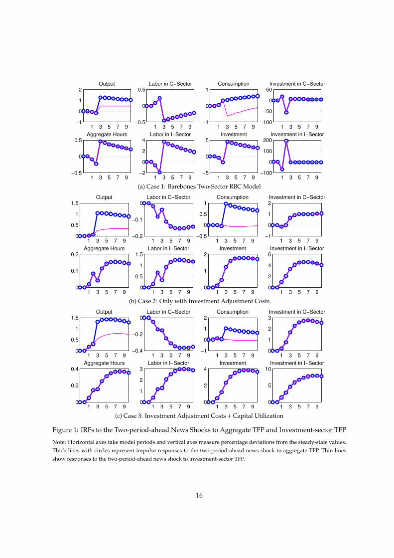
Figure 1 presents impulse responses of model variables to the two-period-ahead news shocks

to aggregate TFP and investment-sector TFP. The timing of the news shock we consider is as follows.

At time zero, the economy is in the steady state. At time one, a news shock arrives. Agents learn that

there will be a one-percent temporary increase in aggregate TFP, A

t

, or investment-sector TFP, z

i,t, two

periods later (at time three), with a persistent parameter equal to 0.95. Note that the dynamic path of

the economy after the anticipated shock materializes corresponds to the one that the economy would

follow in response to a contemporaneous shock. Therefore, Figure 1 allows us to show the ability of

our model to generate the sectoral co-movement to both anticipated and unanticipated shocks. The

thick lines with circles represent dynamic responses of the variables to the anticipated aggregate TFP

shocks, and the thin lines denote those to the anticipated investment-specific technology shocks.12Horvath (2000) uses the fact that relative labor hour percentage changes in one sector are related to relative labor’s

share percentage changes in that sector by the elasticity ✓/(✓ + 1). He estimates this elasticity from an ordinary leastsquare regression of the change in the relative labor supply on the change in the relative labor share using sectoral U.S.data, and finds ✓ = 0.9996, with a standard error of 0.0027.

13This value is a lower bound on the Frisch elasticity used in existing literature. Jaimovich and Rebelo (2009) assume arelatively elastic labor supply. They set ⌘ to 2.5. As (11) shows, setting ⌘ to 2.5 would be favorable to our results becauseit would expand the range of ✓, consistent with sectoral labor co-movement.

15

1 3 5 7 9−1

0

1

2Output

1 3 5 7 9−0.5

0

0.5Labor in C−Sector

1 3 5 7 9−1

0

1Consumption

1 3 5 7 9−100

−50

0

50Investment in C−Sector

1 3 5 7 9−0.5

0

0.5Aggregate Hours

1 3 5 7 9−2

0

2

4Labor in I−Sector

1 3 5 7 9−5

0

5Investment

1 3 5 7 9−100

0

100

200Investment in I−Sector

(a) Case 1: Barebones Two-Sector RBC Model

1 3 5 7 90

0.5

1

1.5Output

1 3 5 7 9−0.2

−0.1

0Labor in C−Sector

1 3 5 7 9−0.5

0

0.5

1Consumption

1 3 5 7 9−1

0

1


1 3 5 7 90

0.1

0.2Aggregate Hours

1 3 5 7 90

0.5

1

1.5Labor in I−Sector

1 3 5 7 90

1

2Investment

1 3 5 7 90

2

4


(b) Case 2: Only with Investment Adjustment Costs

1 3 5 7 90

0.5

1

1.5Output

1 3 5 7 9−0.4

−0.2

0Labor in C−Sector

1 3 5 7 9−1

0

1

2Consumption

1 3 5 7 90

1

2


1 3 5 7 90

0.2

0.4Aggregate Hours

1 3 5 7 90

1

2


1 3 5 7 90

2

4Investment

1 3 5 7 90

5


(c) Case 3: Investment Adjustment Costs + Capital Utilization

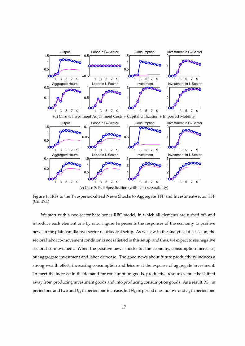
Figure 1: IRFs to the Two-period-ahead News Shocks to Aggregate TFP and Investment-sector TFP

Note: Horizontal axes take model periods and vertical axes measure percentage deviations from the steady-state values.Thick lines with circles represent impulse responses to the two-period-ahead news shock to aggregate TFP. Thin linesshow responses to the two-period-ahead news shock to investment-sector TFP.

16

1 3 5 7 90

0.5

1

1.5Output

1 3 5 7 9−0.5

0


1 3 5 7 90

0.5

1

1.5Consumption

1 3 5 7 90

1


1 3 5 7 90

0.1

0.2Aggregate Hours

1 3 5 7 90

0.5


1 3 5 7 90

1

2Investment

1 3 5 7 90

2


(d) Case 4: Investment Adjustment Costs + Capital Utilization + Imperfect Mobility

1 3 5 7 90

0.5

1

1.5Output

1 3 5 7 90

0.05


1 3 5 7 90

0.5

1Consumption

1 3 5 7 90

1


1 3 5 7 90

0.2

0.4Aggregate Hours

1 3 5 7 90

0.5

1

1.5Labor in I−Sector

1 3 5 7 90

1

2

3Investment

1 3 5 7 90

2

4


(e) Case 5: Full Specification (with Non-separability)

Figure 1: IRFs to the Two-period-ahead News Shocks to Aggregate TFP and Investment-sector TFP(Cont’d.)

We start with a two-sector bare bones RBC model, in which all elements are turned o↵, and

introduce each element one by one. Figure 1a presents the responses of the economy to positive

news in the plain vanilla two-sector neoclassical setup. As we saw in the analytical discussion, the

sectoral labor co-movement condition is not satisfied in this setup, and thus, we expect to see negative

sectoral co-movement. When the positive news shocks hit the economy, consumption increases,

but aggregate investment and labor decrease. The good news about future productivity induces a

strong wealth e↵ect, increasing consumption and leisure at the expense of aggregate investment.

To meet the increase in the demand for consumption goods, productive resources must be shifted

away from producing investment goods and into producing consumption goods. As a result, N

c,t in

period one and two and I

c,t in period one increase, but N

i,t in period one and two and I

i,t in period one

17

decrease. Until the positive news shocks materialize at time three, aggregate output barely moves,

since increases in consumption are o↵set by drops in investment. The dynamics of this economy

after the news shocks materialize is identical to that of contemporaneous shocks. Since the sectoral

labor co-movement condition does not hold, the negative sectoral co-movement of labor persists. As

Christiano and Fitzgerald (1998) show, this is the classical sectoral co-movement problem associated

with aggregate, contemporanesous TFP shocks that most of neoclassical business cycles models

su↵er from. For investment-specific technology shocks, the negative sectoral co-movement of hours

worked is translated into the negative sectoral output co-movement after the positive anticipated

investment-specific technology shocks materialize in period three. This negative co-movement

problem between consumption and investment in response to contemporaneous investment-specific

technology shocks has been emphasized by Greenwood et al. (2000). Since there are no costs to

adjusting investment, sectoral investments exhibit an extremely large response to the shocks.

We then introduce investment adjustment costs to the two-sector standard RBC model, leaving

other features of the model turned o↵. Figure 1b displays the responses of the economy to the positive

news shock. While consumption declines following the positive news shock, the adjustment costs to

investment in each sector generate a positive response in aggregate hours worked and investment.

As Jaimovich and Rebelo (2009) clearly explain, adjustment costs to investment make it optimal to

smooth investment over time and, thus, provide a reduced-form representation of the economic

mechanism that would operate immediately in response to the positive news shock. With high

enough adjustment costs, the intertemporal substitution e↵ect might dominate the wealth e↵ect, so

that aggregate hours worked and investment might increase in response to the positive news shock.

In fact, this is exactly what is happening in Figure 1b and they respond positively to the news shocks

in the first two periods. However, the sectoral co-movement problem still exists. That is, hours

worked and investment in each sector move in the opposite direction. However, adjustment costs

to investment in each sector seem to alleviate the problem of sectoral co-movement in investment.

Even though I

c,t and I

i,t do not move together in response to the news shocks in the initial period,

the di↵erence between these two is substantially reduced compared to the standard two-sector

RBC model. As before, the negative sectoral co-movement of labor still persists after news shocks

materialize.

In addition to the investment adjustment costs, we now allow the rate of capital utilization in

18

each sector to vary, maintaining the assumption of perfect labor mobility and separable preferences.

Figure 1c depicts the responses of the economy with the investment adjustment costs and the

variable capital utilization. The most significant change in the reaction of the economy is that

the variable capital utilization combined with the investment adjustment costs generates the co-

movement in sectoral investment. Both I

c,t and I

i,t increase in response to the positive news shocks.

However, the investment adjustment costs and the variable capital utilization do not solve the

problem of co-movement in hours worked across the consumption and investment sectors. There

still exists the co-movement problem, that is that N

c,t and N

i,t move in the opposite direction.

Furthermore, consumption still stagnates until the positive news materializes at time three, and

aggregate investment increases in periods one and two. Hence, the model still fails to generate the

strong co-movement in output across two sectors.

Along with variable capital utilization and investment adjustment costs, we now introduce

friction in labor allocation, maintaining the separable preferences. Figure 1d portrays the responses

of the economy with the separable preferences. It clearly shows that frictions in labor mobility

significantly alleviate the problem of co-movement in hours worked across sectors. Here, N

c,t has

decreased before the friction in labor mobility is introduced, but now it does not respond at all to

the news shocks. This invariant response of hours worked in the consumption sector is already

anticipated by (11). Given our parameterization that ✓ = ⌘ = 1 and � = 1, (11) implies that N

c,t

does not change in response to the news shock. Note that (11) also applies to the contemporaneous

shocks, N

c,t also does not move after news shocks materialize.

Finally, Figure 1e presents the response of the economy to the news shocks with the full

specification, allowing for non-separable preferences between consumption and labor. There is an

expansion in periods one and two in response to both positive news about aggregate TFP (At

) and

sectoral TFP in the investment sector (zi,t). Output, employment, and investment in the consumption

and investment sectors increase together in periods one and two, even though the positive shock

only materializes in period three. Therefore, our model successfully produces the business cycle

co-movement in response to news about future values of A

t

and z

i,t. Furthermore, in our model,

output, employment, and investment in the consumption and investment sectors continue to move

together, even after the shock materializes (in period three). This implies that our model can also

generate the sectoral co-movement in those variables in response to contemporaneous aggregate

19

1 3 5 7 90

0.5

1

1.5Output

1 3 5 7 9−0.05

0


1 3 5 7 90

0.5

1

1.5Consumption

1 3 5 7 9−1

0

1


1 3 5 7 9−0.5

0

0.5Aggregate Hours

1 3 5 7 9−0.5

0

0.5


1 3 5 7 9−2

0

2

4Investment

1 3 5 7 90

2

4


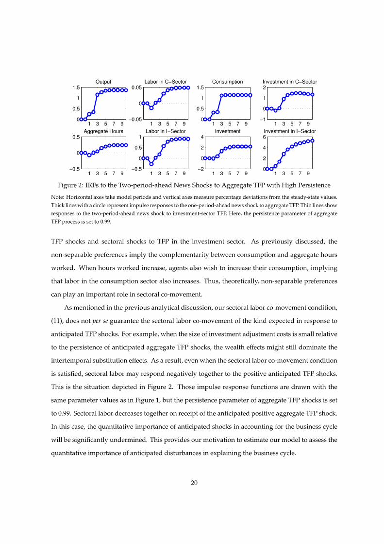
Figure 2: IRFs to the Two-period-ahead News Shocks to Aggregate TFP with High Persistence

Note: Horizontal axes take model periods and vertical axes measure percentage deviations from the steady-state values.Thick lines with a circle represent impulse responses to the one-period-ahead news shock to aggregate TFP. Thin lines showresponses to the two-period-ahead news shock to investment-sector TFP. Here, the persistence parameter of aggregateTFP process is set to 0.99.

TFP shocks and sectoral shocks to TFP in the investment sector. As previously discussed, the

non-separable preferences imply the complementarity between consumption and aggregate hours

worked. When hours worked increase, agents also wish to increase their consumption, implying

that labor in the consumption sector also increases. Thus, theoretically, non-separable preferences

can play an important role in sectoral co-movement.

As mentioned in the previous analytical discussion, our sectoral labor co-movement condition,

(11), does not per se guarantee the sectoral labor co-movement of the kind expected in response to

anticipated TFP shocks. For example, when the size of investment adjustment costs is small relative

to the persistence of anticipated aggregate TFP shocks, the wealth e↵ects might still dominate the

intertemporal substitution e↵ects. As a result, even when the sectoral labor co-movement condition

is satisfied, sectoral labor may respond negatively together to the positive anticipated TFP shocks.

This is the situation depicted in Figure 2. Those impulse response functions are drawn with the

same parameter values as in Figure 1, but the persistence parameter of aggregate TFP shocks is set

to 0.99. Sectoral labor decreases together on receipt of the anticipated positive aggregate TFP shock.

In this case, the quantitative importance of anticipated shocks in accounting for the business cycle

will be significantly undermined. This provides our motivation to estimate our model to assess the

quantitative importance of anticipated disturbances in explaining the business cycle.

20

4 Estimation

We take our model to the data using Bayesian methods and estimate model parameters. Of particular

importance among the estimated parameters are those governing the degree of inter-sectoral labor

mobility and non-separability, the elasticity of marginal cost of capital utilization, the size of invest-

ment adjustment costs, and those defining the stochastic processes of anticipated and unanticipated

innovations.

4.1 Specification

We now formally describe the exogenous structural disturbances that drive the business cycles in our

model. Hence, our model of the business cycle is composed of six structural shocks: the stationary

TFP shock (at

), the non-stationary TFP shock (At

), the stationary investment-specific technology

shock (zi,t), the two sectoral wage markup shocks (µ

c,t and µi,t), and the preference shock (b

t

).

Following Fujiwara et al. (2011) and Schmitt-Grohe and Uribe (2008), we model the information

structure on the contemporaneous and anticipated shocks in the following way. We assume that all

exogenous shocks, f

t

= a

t

, gt

(⌘ A

t

/At�1), z

i,t, µc,t, µi,t, except for b

t

, evolve over time according to the

following law of motion:

log( f

t

/ f ) = ⇢f

log( f

t�1/ f ) + v

0f ,t + v

1f ,t�1 + v

2f ,t�2 + v

3f ,t�3 + v

4f ,t�4, (13)

where v

h

f ,t, for h = 0, 1, · · · , 4, and f = {a, g, zi

, µc

, µi

} is assumed to be an i.i.d. normal disturbance a

with mean of zero and a standard deviation of �h

f

. Then, v

0f ,t are the unanticipated contemporaneous

shocks and v

h

f ,t, for h = 1, · · · , 4 represent the h-period-ahead news shock anticipated at time t.

Here, we assume that agents receive the news up to four periods ahead. This is consistent with

Schmitt-Grohe and Uribe (2012), who find that four-quarter-ahead anticipated shocks are the most

important driver of business cycles in the estimated one-sector version of Jaimovich and Rebelo

(2009). For preference shocks, we do not introduce anticipated shocks and assume an AR(1) process

with contemporaneous shocks, namely, log(bt

/b) = ⇢b

log(bt�1/b) + v

0b,t, with v

0b,t ⇠ i.i.d. N(0, (�0

b

)2).

In our model, consumption, aggregate investment, sectoral investment, sectoral capital, and

sectoral real wages fluctuate around a stochastic balanced growth path, since the exogenous forcing

21

process, A

t

, displays a stochastic trend. We perform a stationarity-inducing transformation of

the endogenous variables by dividing them by their trend component. We then compute the

non-stochastic steady state of the transformed model and log-linearize it around this steady state.

Finally, we solve the resulting linear system of rational expectation equations to obtain its state-space

representation. This representation forms the basis for the estimation procedure, which is discussed

in the next subsection.

In order to incorporate sectoral characteristics into the estimation, we utilize sector-specific

data, rather than aggregate data. Here, we will use the following five observables: the real per

capita consumption growth (dC

t

), the growth rate of hours worked in the consumption sector (dh

c,t),

the real per capita investment growth (dI

t

), the growth rate of hours worked in consumption sector

(dh

i,t), and the growth rate of aggregate real wage (dw

t

).14 Sectoral labor data are constructed from

the Current Employment Statistics of the BLS. The Appendix describes the data construction in

detail. The sample period starts from 1964:II and ends at 2013:IV. All variables are de-meaned

before the estimation.

More specifically, the measurement equations in a state-space representation relate observable

variables and the model counterpart in the following way:

dC

t

= C

t

� C

t�1, (14)

dh

c,t = N

c,t � N

c,t�1, (15)

dI

t

= I

t

� I

t�1, (16)

dh

i,t = N

i,t � N

i,t�1, (17)

dw

t

= s

c

(wc,t � w

c,t�1) + (1 � s

c

)(wi,t � w

i,t�1), (18)

where s

c

is the share of the consumption sector.

We fix some of the structural parameters. We set the discount factor (�) to 0.985, and the capital

share (↵) to 0.36. We assume that the steady-state depreciation rate at the steady state is 0.025, which

is the same in both sectors. These values are adapted from the values used in Jaimovich and Rebelo

(2009), and are also used for previous simulations. The steady-state consumption share is set to14We assume that the consumption sector consists of firms producing non-durable goods and services and that the

investment sector produces durable goods and goods used for non-residential and residential investment.

22

0.78, which is the average over the sample period. The steady-state wage markup in each sector is

assume to be the same, and fixed at 1.15.

The left side of Table 1 summarizes the prior distributions we employ. We use a Gamma

distribution for 1/⌘ with mean 1 and standard deviation of 0.25. We assume a Gamma distribution

for 1/✓ with mean 1 and standard deviation of 0.5. This choice of the prior mean is consistent

with the estimate of Horvath (2000). We use a Beta distribution for � with mean 0.5 and standard

deviation of 0.2. This prior mean is much more conservative than the posterior mean obtained in

the two-sector model of Kim and Katayama (2013) and the non-separability parameter found in

Guerron-Quintana (2008). Based on the prior distributions of 1/⌘, 1/✓, and �, in the absence of

internal habit formation, the implied prior probability of satisfying the normality condition is about

89% and that of satisfying the sectoral co-movement condition is roughly 73%.

Prior distributions of h, j

⌘ �00 (u

j

)uj

�0 (uj

) for j = c, i, and �00 are adopted from Schmitt-Grohe and

Uribe (2010). The prior distribution of h is a Beta distribution with mean 0.5 and standard deviation

0.2. We assume that j

is distributed as an Inverse Gamma distribution with mean 1 and standard

deviation of 1, and that �00 follows a Gamma distribution with mean 4 and standard deviation of 1.

We use a Gamma distribution with mean 1.65 and standard deviation of 1 for a prior distribution

of g⇥ 400. We use a Beta distribution as a prior for the persistence parameters. The prior means for

⇢a

and ⇢b

are assumed to be 0.7, and those for ⇢z

i

, ⇢µc

, and ⇢µi

are set to 0.5. The prior mean of ⇢g

is

assumed to be 0.2. All standard deviations for ⇢’s are set to 0.2.

For prior distributions of the standard deviations of exogenous shocks in the model, we use

Gamma distributions.15 As discussed in Schmitt-Grohe and Uribe (2012), this choice imposes a

conservative stance on the importance of anticipated shocks. This is because, unlike the typical

Inverse Gamma distributions, the Gamma distribution allows a positive density at zero. That is, our

prior incorporates the possibility that the news shocks are not operating. Furthermore, we impose

the 75-percent rule on the prior means of the standard deviations of the anticipated shocks, as in

Schmitt-Grohe and Uribe (2012). Our priors restrict the variance of the unanticipated shock accounts

to 75 percent of the total variance of the shock, and we assume that the four types of anticipated

shocks are equally important to account for the remaining portion of the total variance. Our choice

of priors are more conservative than those used in Fujiwara et al. (2011), which put equal weights15The only exception is that of the discount factor shock, which uses the typical inverse Gamma distribution.

23

Table 1: Prior and Posterior Distributions for the Benchmark Model

Prior Distribution Posterior DistributionParameter Distribution Mean Std. Dev. Mean 5 % 95 %

1/⌘ Gamma 1 0.25 0.8372 0.6386 1.03661/✓ Gamma 1 0.5 3.3835 2.8139 3.9424� Beta 0.5 0.2 0.7389 0.5607 0.9376h Beta 0.5 0.2 0.3216 0.2375 0.4066

c

Inv. Gamma 1 1 4.8452 3.7056 5.9234

i

Inv. Gamma 1 1 1.0719 0.3888 1.7699�00 (1) Gamma 4 1 1.3198 1.0344 1.6030

g ⇥ 400 Gamma 1.65 1 0.6722 0.0954 1.2403⇢

a

Beta 0.7 0.2 0.9682 0.9352 0.9999⇢

g

Beta 0.2 0.2 0.4687 0.1037 0.7784⇢

i

Beta 0.5 0.2 0.9458 0.9206 0.9709⇢

b

Beta 0.7 0.2 0.9322 0.9075 0.9547⇢µ

c

Beta 0.5 0.2 0.9854 0.9759 0.9958⇢µ

i

Beta 0.5 0.2 0.9424 0.9113 0.9733�0

a

Gamma 0.015 0.015 0.0030 0.0024 0.0037�1

a

Gamma 0.0043 0.0043 0.0007 0.0000 0.0015�2

a

Gamma 0.0043 0.0043 0.0006 0.0000 0.0013�3

a

Gamma 0.0043 0.0043 0.0007 0.0000 0.0014�4

a

Gamma 0.0043 0.0043 0.0007 0.0000 0.0014�0

g

Gamma 0.015 0.015 0.0011 0.0000 0.0021�1

g

Gamma 0.0043 0.0043 0.0009 0.0000 0.0019�2

g

Gamma 0.0043 0.0043 0.0012 0.0000 0.0024�3

g

Gamma 0.0043 0.0043 0.0012 0.0000 0.0024�4

g

Gamma 0.0043 0.0043 0.0013 0.0000 0.0024�0

i

Gamma 0.015 0.015 0.0146 0.0132 0.0162�1

i

Gamma 0.0043 0.0043 0.0013 0.0000 0.0028�2

i

Gamma 0.0043 0.0043 0.0016 0.0000 0.0033�3

i

Gamma 0.0043 0.0043 0.0015 0.0000 0.0032�4

i

Gamma 0.0043 0.0043 0.0016 0.0000 0.0035�

b

Inv. Gamma 0.0173 0.0173 0.0635 0.0531 0.0734�0µ

c

Gamma 0.015 0.015 0.0025 0.0000 0.0050�1µ

c

Gamma 0.0043 0.0043 0.0023 0.0000 0.0049�2µ

c

Gamma 0.0043 0.0043 0.0030 0.0000 0.0060�3µ

c

Gamma 0.0043 0.0043 0.0027 0.0000 0.0057�4µ

c

Gamma 0.0043 0.0043 0.0030 0.0000 0.0064�0µ

i

Gamma 0.015 0.015 0.0068 0.0000 0.0144�1µ

i

Gamma 0.0043 0.0043 0.0296 0.0000 0.0576�2µ

i

Gamma 0.0043 0.0043 0.0255 0.0000 0.0586�3µ

i

Gamma 0.0043 0.0043 0.0038 0.0000 0.0087�4µ

i

Gamma 0.0043 0.0043 0.0126 0.0000 0.0381Log Marginal Density 3361.21

Note: The posterior distributions are obtained using the random walk Metropolis–Hastings algorithm with 300,000 draws (the first 10% of draws are discarded as a burn-inperiod). We use the modified Harmonic mean estimator of Geweke (1999) to obtain thelog marginal density.

24

on anticipated and contemporaneous components in terms of the role of the news shocks.

4.2 Posterior Estimates

We find the posterior mode numerically and use it as a starting point of the random-walk Metropolis–

Hastings algorithm. The subsequent results are all based on 300,000 Metropolis–Hastings draws.16

We adjust the scaling factor in the Metropolis–Hastings algorithm such that the acceptance rate

becomes about 25%.

The right side of Table 1 presents the posterior distributions of the parameters in our model.

The posterior mean of 1/✓ is estimated to be 3.38 and, thus, the implied estimates of ✓ are much

smaller than the one estimated by Horvath (2000). This suggests a substantial degree of inter-

sectoral labor immobility in the labor market. The posterior mean of � is estimated to be 0.74, so

that the degree of non-separability in the utility function is moderate. Our estimate of the degree

of the non-separability is smaller than that reported in Kim and Katayama (2013) and closer to the

estimates of Smets and Wouters (2007) and Fujiwara et al. (2011). The estimate of the posterior

mean of 1/⌘ is 0.84, implying that the Frisch elasticity of labor supply is about 1.19. Therefore,

our estimates of ✓, �, and ⌘ satisfy the sectoral labor co-movement condition (11) and a significant

degree of inter-sectoral labor immobility plays a crucial role in attaining the condition. Note that

the sectoral labor co-movement condition (11) is derived in the absence of habit formation, and

also that it is not su�cient to ensure the sectoral co-movement of hours worked in response to the

consumption-sector wage markup shock. It turns out that our estimated two-sector neoclassical

DSGE model with habit formation does display the sectoral co-movement of hours worked, as

described below.

Turning to the estimates of the remaining parameters, the estimated degree of internal habit

formation, h, is 0.32. This estimate is much lower than found by earlier DSGE-based Bayesian

econometric studies. However, this is consistent with the micro-evidence reported by Dynan (2000)

and Ravina (2007), and the impulse-response-matching estimate in Guerron-Quintana (2008). The

investment adjustment cost parameter, �00 , is also estimated to be significantly smaller than those

in DSGE-based macroeconometric literature. In particular, while Schmitt-Grohe and Uribe (2012)

estimate �00 to be equal to 9.11 in their one-sector version of the Jaimovich and Rebelo (2009)16The first 30,000 draws are discarded as a burn-in period.

25

neoclassical DSGE model, our estimate of �00 is 1.32.

The low estimates of h and �00 might be attributable to the sectoral labor co-movement condi-

tion, (11), which makes hours growth in both sectors mimic each other. The persistent pattern of

investment-sector hours growth due to the presence of investment adjustment costs is transmitted

to the hours growth in the consumption sector through the sectoral labor co-movement condition.

This in turn makes it possible for our model to match the observed positive autocorrelation of

consumption growth with a smaller degree of habit formation. The same logic can be applied

to explain the low estimate of �00 . The presence of habit formation leads to a persistent process

of consumption-sector hours growth, resulting in a similar persistent process of investment-sector

hours growth through the sectoral labor co-movement condition. Again, this reduces the magni-

tude of the investment adjustment costs required to match the observed positive autocorrelation of

consumption growth in the data. In Section 5.3, we revisit this aspect and show that even with these

low estimates of h and �00 , our model maintains the ability to match the observed autocorrelations

of consumption and investment growth.

Regarding the elasticity of marginal cost of capital utilization, the estimates of c

and i

display

a substantial sectoral di↵erence. Varying utilization in the consumption sector is much more costly

than in the investment sector. Our estimates of c

and i

seem to capture the property of the data

that investment is much more volatile than consumption. The low estimate of i

makes the level

of utilization highly responsive to shocks, resulting in a powerful amplification of the shocks in

the investment sector. In contrast, the consumption sector does not need as large an amplification

mechanism, resulting in a large estimate of c

.

Finally, the posterior 90% probability intervals of the standard deviations of anticipated shocks

typically contain zero. The only exception is the four-period-ahead investment-sector wage markup

shock. This might suggest a limited role of anticipated shocks in explaining business cycle fluctua-

tions.

4.3 Variance Decomposition

We investigate the quantitative importance of our estimated shocks as sources of business-cycle

fluctuations. Table 2 displays the contribution of all shocks to the unconditional variance of the

26

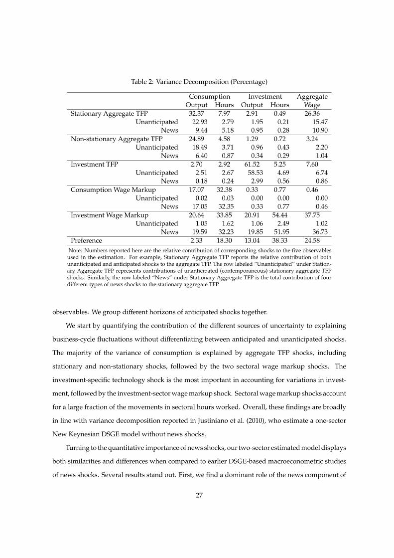
Table 2: Variance Decomposition (Percentage)

Consumption Investment AggregateOutput Hours Output Hours Wage

Stationary Aggregate TFP 32.37 7.97 2.91 0.49 26.36Unanticipated 22.93 2.79 1.95 0.21 15.47

News 9.44 5.18 0.95 0.28 10.90Non-stationary Aggregate TFP 24.89 4.58 1.29 0.72 3.24

Unanticipated 18.49 3.71 0.96 0.43 2.20News 6.40 0.87 0.34 0.29 1.04

Investment TFP 2.70 2.92 61.52 5.25 7.60Unanticipated 2.51 2.67 58.53 4.69 6.74

News 0.18 0.24 2.99 0.56 0.86Consumption Wage Markup 17.07 32.38 0.33 0.77 0.46

Unanticipated 0.02 0.03 0.00 0.00 0.00News 17.05 32.35 0.33 0.77 0.46

Investment Wage Markup 20.64 33.85 20.91 54.44 37.75Unanticipated 1.05 1.62 1.06 2.49 1.02

News 19.59 32.23 19.85 51.95 36.73Preference 2.33 18.30 13.04 38.33 24.58

Note: Numbers reported here are the relative contribution of corresponding shocks to the five observablesused in the estimation. For example, Stationary Aggregate TFP reports the relative contribution of bothunanticipated and anticipated shocks to the aggregate TFP. The row labeled “Unanticipated” under Station-ary Aggregate TFP represents contributions of unanticipated (contemporaneous) stationary aggregate TFPshocks. Similarly, the row labeled “News” under Stationary Aggregate TFP is the total contribution of fourdi↵erent types of news shocks to the stationary aggregate TFP.

observables. We group di↵erent horizons of anticipated shocks together.

We start by quantifying the contribution of the di↵erent sources of uncertainty to explaining

business-cycle fluctuations without di↵erentiating between anticipated and unanticipated shocks.

The majority of the variance of consumption is explained by aggregate TFP shocks, including

stationary and non-stationary shocks, followed by the two sectoral wage markup shocks. The

investment-specific technology shock is the most important in accounting for variations in invest-

ment, followed by the investment-sector wage markup shock. Sectoral wage markup shocks account

for a large fraction of the movements in sectoral hours worked. Overall, these findings are broadly

in line with variance decomposition reported in Justiniano et al. (2010), who estimate a one-sector

New Keynesian DSGE model without news shocks.

Turning to the quantitative importance of news shocks, our two-sector estimated model displays

both similarities and di↵erences when compared to earlier DSGE-based macroeconometric studies

of news shocks. Several results stand out. First, we find a dominant role of the news component of

27

sectoral wage markup shocks in explaining business cycle fluctuations. For example, the combined

two sectoral wage markup news shocks account for about 64.58% and 52.72% of the variation in

hours worked in the consumption and investment sectors, respectively. In contrast, unanticipated

wage markup shocks explain only about 1.65% and 2.49% of the variance of hours worked in the

consumption and investment sectors. It is the news shock components that matter for accounting

for business cycle fluctuations. This is consistent with findings in Khan and Tsoukalas (2012)

and Schmitt-Grohe and Uribe (2012). Quantitatively speaking, the news components of the wage

markup shocks appear to be more important than earlier studies.

Second, the contribution of aggregate TFP news shocks remains relatively small. This is consis-

tent with the findings in earlier studies. For example, the anticipated stationary and non-stationary

aggregate TFP shocks, combined together, account for about 16% of the variance of consumption

growth. This is the value reported in Fujiwara et al. (2011), but is quantitatively larger than those

reported by Khan and Tsoukalas (2012) and Schmitt-Grohe and Uribe (2012).

Third, in our model, the majority of the variation in investment is accounted for by unanticipated

investment-specific technology shocks (with a variance share of 58.53%). The news component of

the investment-specific technology shocks plays virtually no role in explaining business cycles. This

result is similar to that of Khan and Tsoukalas (2012). In contrast, Schmitt-Grohe and Uribe (2012)

report that about 20% of the variance of investment is due to the anticipated component of the

investment-specific technology shocks.

Finally, the di↵erences in the importance of the anticipated shocks relative to Schmitt-Grohe

and Uribe (2012) might be explained by the lower estimates of habit formation and investment ad-

justment costs in our model. As discussed in Section 3.2, a lower value of the investment adjustment

cost parameter dampens the response of investment on receipt of an anticipated investment-specific

technology shock. As a result, our model predicts that the news component of investment-specific

technology shocks has little influence on the variance of investment. In Schmitt-Grohe and Uribe

(2012), a sizable fraction of the variation in investment is attributable to the anticipated investment-

specific technology shocks because of the larger estimate of investment adjustment costs. In contrast,

a decline in the estimated degree of habit persistence results in a more pronounced response of con-

sumption to an anticipated TFP shock. Hence, anticipated TFP shocks play a larger role in explaining

variations in consumption than they do in Schmitt-Grohe and Uribe (2012).

28

5 A Comparison with the Jaimovich and Rebelo (2009) Model

In this section, we evaluate the empirical performance of our model relative to that of a two-

sector version of the Jaimovich and Rebelo (2009) model. Jaimovich and Rebelo (2009) introduce

preferences featuring a parameter that governs the wealth elasticity of labor supply, and show that

wealth e↵ects on the labor supply play a crucial role in determining sectoral labor co-movement. We

estimate a two-sector version of the Jaimovich and Rebelo (2009) model, and investigate whether

our proposed mechanism of generating sectoral labor co-movement (i.e., imperfect inter-sectoral

mobility) is favored by the data, as against using the Jaimovich–Rebelo preferences.17

5.1 Specification

The novel feature in Jaimovich and Rebelo (2009) is to introduce a particular class of preferences that

has a parameter governing the size of the wealth e↵ect on labor supply. Following Schmitt-Grohe

and Uribe (2012), we modify the Jaimovich–Rebelo preferences to allow for internal habit formation

in consumption. In particular, the habit-augmented Jaimovich–Rebelo utility function is given by

U(Ct

� hC

t�1,Nt

) = log⇣C

t

� hC

t�1 � N

⇣t

X

t

⌘, (19)

where X

t

evolves according to

X

t

= (Ct

� hC

t�1)�X

1��t�1 . (20)

The parameter ⇣ > 1 determines the Frisch elasticity of labor supply in the special case in which

� = h = 0. The parameter � 2 [0, 1] controls the size of the wealth e↵ect on the labor supply.

When � = 0, the period utility function corresponds to the preference specification proposed by

Greenwood et al. (1988), in the absence of habit formation. This special case induces a zero wealth

e↵ect on the labor supply, referred to as the GHH preferences. As � increases, the wealth elasticity

of labor supply increases. When � = 1, the period utility function reduces to the standard King–

Plosser–Rebelo preferences. Finally, as in Jaimovich and Rebelo (2009), labor is perfectly mobile

between two sectors (i.e., N

t

= N

c,t + N

i,t). The rest of the model structure is identical to that

presented in Section 2.17Schmitt-Grohe and Uribe (2012) estimate the one-sector version of the Jaimovich and Rebelo (2009) model.

29

We assume that the same exogenous structural disturbances drive the business cycles, as be-

fore. We also perform a stationary-inducing transformation of the endogenous variables before the

Bayesian estimation. We follow the prior distributions used in Schmitt-Grohe and Uribe (2010) for

the structural parameters absent in our model, namely � and ⇣. We adopt a uniform prior distribu-

tion over 0 and 1 for �, controlling the size of the labor-supply wealth e↵ect, and a Gamma prior

distribution with mean 4 and standard deviation of 1 for ⇣, controlling the Frisch labor supply elas-

ticity. The prior distributions for the rest of the parameters are identical to those used in estimating

our model. The same observables and measurement equations (14)-(18) are used in the Bayesian

estimation.

5.2 Posterior Estimates

Table 3 presents the posterior distributions of the parameters in the two-sector version of Jaimovich

and Rebelo (2009), together with the associated prior distributions. Overall, our estimates of the

two-sector version of the Jaimovich–Rebelo model are in line with Schmitt-Grohe and Uribe (2012),

who estimate a one-sector version. The posterior mean of � is estimated to be very close to zero.

This estimate implies that, in the absence of habit formation, the model would display a labor

supply schedule with a near-zero wealth e↵ect of labor supply. The habit persistent parameter, h,

is estimated to be around 0.99. The estimate of h is similar to the one reported in Schmitt-Grohe

and Uribe (2012), but it is substantially larger than our estimate with the limited labor mobility

presented in Section 4.2. The parameter ⇣, governing the Frisch labor elasticity, is estimated to be

around 1.71, significantly smaller than the estimate of Schmitt-Grohe and Uribe (2012) (4.74). The

investment adjustment cost parameter, �00 , is estimated to be around 2.85, which lies between our

estimate and that of Schmitt-Grohe and Uribe (2012). As in our estimated model, the estimates of

c

and i

display a substantial sectoral di↵erence, implying that it is much more costly to vary the

rate of capital utilization in the consumption sector than in the investment sector.

5.3 Model Comparison

We now quantitatively compare the two competing models that might display the sectoral labor

co-movement. By using the Bayes factor, we can formally compare the performance of our model

30

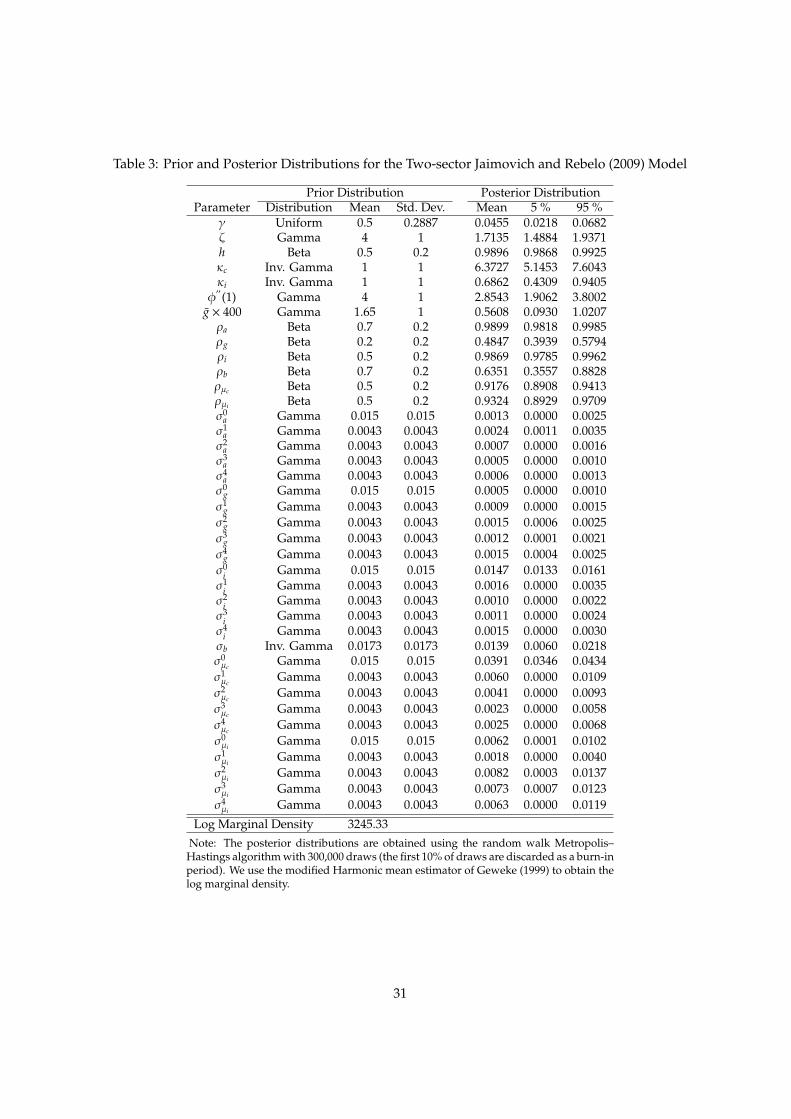
Table 3: Prior and Posterior Distributions for the Two-sector Jaimovich and Rebelo (2009) Model

Prior Distribution Posterior DistributionParameter Distribution Mean Std. Dev. Mean 5 % 95 %

� Uniform 0.5 0.2887 0.0455 0.0218 0.0682⇣ Gamma 4 1 1.7135 1.4884 1.9371h Beta 0.5 0.2 0.9896 0.9868 0.9925

c

Inv. Gamma 1 1 6.3727 5.1453 7.6043

i

Inv. Gamma 1 1 0.6862 0.4309 0.9405�00 (1) Gamma 4 1 2.8543 1.9062 3.8002

g ⇥ 400 Gamma 1.65 1 0.5608 0.0930 1.0207⇢

a

Beta 0.7 0.2 0.9899 0.9818 0.9985⇢

g

Beta 0.2 0.2 0.4847 0.3939 0.5794⇢

i

Beta 0.5 0.2 0.9869 0.9785 0.9962⇢

b

Beta 0.7 0.2 0.6351 0.3557 0.8828⇢µ

c

Beta 0.5 0.2 0.9176 0.8908 0.9413⇢µ

i

Beta 0.5 0.2 0.9324 0.8929 0.9709�0

a

Gamma 0.015 0.015 0.0013 0.0000 0.0025�1

a

Gamma 0.0043 0.0043 0.0024 0.0011 0.0035�2

a

Gamma 0.0043 0.0043 0.0007 0.0000 0.0016�3

a

Gamma 0.0043 0.0043 0.0005 0.0000 0.0010�4

a

Gamma 0.0043 0.0043 0.0006 0.0000 0.0013�0

g

Gamma 0.015 0.015 0.0005 0.0000 0.0010�1

g

Gamma 0.0043 0.0043 0.0009 0.0000 0.0015�2

g

Gamma 0.0043 0.0043 0.0015 0.0006 0.0025�3

g

Gamma 0.0043 0.0043 0.0012 0.0001 0.0021�4

g

Gamma 0.0043 0.0043 0.0015 0.0004 0.0025�0

i

Gamma 0.015 0.015 0.0147 0.0133 0.0161�1

i

Gamma 0.0043 0.0043 0.0016 0.0000 0.0035�2

i

Gamma 0.0043 0.0043 0.0010 0.0000 0.0022�3

i

Gamma 0.0043 0.0043 0.0011 0.0000 0.0024�4

i

Gamma 0.0043 0.0043 0.0015 0.0000 0.0030�

b

Inv. Gamma 0.0173 0.0173 0.0139 0.0060 0.0218�0µ

c

Gamma 0.015 0.015 0.0391 0.0346 0.0434�1µ

c

Gamma 0.0043 0.0043 0.0060 0.0000 0.0109�2µ

c

Gamma 0.0043 0.0043 0.0041 0.0000 0.0093�3µ

c

Gamma 0.0043 0.0043 0.0023 0.0000 0.0058�4µ

c

Gamma 0.0043 0.0043 0.0025 0.0000 0.0068�0µ

i

Gamma 0.015 0.015 0.0062 0.0001 0.0102�1µ

i

Gamma 0.0043 0.0043 0.0018 0.0000 0.0040�2µ

i

Gamma 0.0043 0.0043 0.0082 0.0003 0.0137�3µ

i

Gamma 0.0043 0.0043 0.0073 0.0007 0.0123�4µ

i

Gamma 0.0043 0.0043 0.0063 0.0000 0.0119Log Marginal Density 3245.33

Note: The posterior distributions are obtained using the random walk Metropolis–Hastings algorithm with 300,000 draws (the first 10% of draws are discarded as a burn-inperiod). We use the modified Harmonic mean estimator of Geweke (1999) to obtain thelog marginal density.

31

with that of the Jaimovich–Rebelo model in fitting the data. The Bayes factor tells us the strength of

evidence provided by the data. We use the modified Harmonic mean estimator of Geweke (1999)

to obtain the log marginal density. The log data density associated with our model is 3360.38, as

reported in Table 1, whereas that of the Jaimovich and Rebelo (2009) model, shown in Table 3, is

3245.33. In order to choose the Jaimovich–Rebelo specification over ours, we need to assign a prior

probability of the Jaimovich–Rebelo preferences exp(115.88) ⇡ 2.12⇥1050 times larger than that over

the non-separable King–Plosser–Rebelo preferences, with imperfect inter-sectoral labor mobility.

This di↵erence seems to be overwhelmingly large, which suggests that the data decisively support

our model.

To better understand why the empirical fit of our model is superior to that of the Jaimovich–

Rebelo specification, we compare the second moments predicted by our model and their model.

Table 4 compares the standard deviations, autocorrelations, and cross-correlations predicted by

our model with the estimated two-sector Jaimovich–Rebelo model. Overall, our estimated model

matches the empirical second moments well. It replicates the observed volatility in consumption,

investment, hours worked in consumption and investment sectors, and real wages. The model

also e↵ectively captures the autocorrelations of consumption growth, investment growth, and real

wages growth. As mentioned above, even with low estimates of habit persistence and investment

adjustment costs, our model is capable of matching the positive autocorrelations of consumption

growth and investment growth in the data. However, there is a discrepancy between the model pre-

diction and the data. The predicted autocorrelations of hours growth in both sectors are somewhat

weaker than in the data.

The most noticeable di↵erence between the two models stems from the ability to replicate the

observed sectoral co-movement of hours worked and output. Our estimated model produces the

observed positive correlations between sectoral labors and between sectoral outputs. As mentioned

earlier, it has been a challenge for multi-sector neoclassical DSGE models to produce the sectoral

co-movement of output and hours worked. The estimated model overcomes this challenge and

successfully generates the sectoral co-movement.

In contrast, the estimated Jaimovich–Rebelo model does not capture the positive correlations

of sectoral hours worked and sectoral outputs well. This might be an important factor contribut-

ing to the data favoring our model over the Jaimovich-Rebelo model. In other dimensions, our

32

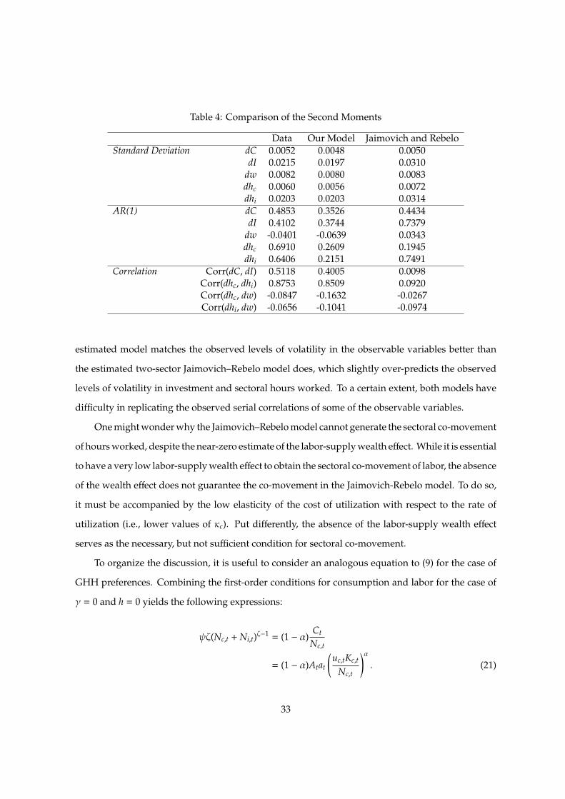
Table 4: Comparison of the Second Moments

Data Our Model Jaimovich and RebeloStandard Deviation dC 0.0052 0.0048 0.0050

dI 0.0215 0.0197 0.0310dw 0.0082 0.0080 0.0083dh

c

0.0060 0.0056 0.0072dh

i

0.0203 0.0203 0.0314AR(1) dC 0.4853 0.3526 0.4434

dI 0.4102 0.3744 0.7379dw -0.0401 -0.0639 0.0343dh

c

0.6910 0.2609 0.1945dh

i

0.6406 0.2151 0.7491Correlation Corr(dC, dI) 0.5118 0.4005 0.0098

Corr(dh

c

, dh

i

) 0.8753 0.8509 0.0920Corr(dh

c

, dw) -0.0847 -0.1632 -0.0267Corr(dh

i

, dw) -0.0656 -0.1041 -0.0974

estimated model matches the observed levels of volatility in the observable variables better than

the estimated two-sector Jaimovich–Rebelo model does, which slightly over-predicts the observed

levels of volatility in investment and sectoral hours worked. To a certain extent, both models have

di�culty in replicating the observed serial correlations of some of the observable variables.

One might wonder why the Jaimovich–Rebelo model cannot generate the sectoral co-movement

of hours worked, despite the near-zero estimate of the labor-supply wealth e↵ect. While it is essential

to have a very low labor-supply wealth e↵ect to obtain the sectoral co-movement of labor, the absence

of the wealth e↵ect does not guarantee the co-movement in the Jaimovich-Rebelo model. To do so,

it must be accompanied by the low elasticity of the cost of utilization with respect to the rate of

utilization (i.e., lower values of c

). Put di↵erently, the absence of the labor-supply wealth e↵ect

serves as the necessary, but not su�cient condition for sectoral co-movement.

To organize the discussion, it is useful to consider an analogous equation to (9) for the case of

GHH preferences. Combining the first-order conditions for consumption and labor for the case of

� = 0 and h = 0 yields the following expressions:

⇣(Nc,t +N

i,t)⇣�1 = (1 � ↵)C

t

N

c,t

= (1 � ↵)At

a

t

u

c,tKc,t

N

c,t

!↵. (21)

33

Equation (21) shows that it is possible for N

c,t and N

i,t to move in the same direction. However,

at the same time, a careful inspection also shows that higher values of c

make it more di�cult

for N

c,t and N

i,t to move in the same direction. Suppose, for example, that N

i,t increases, so that

the marginal disutility of work increases. Capital utilization in the consumption sector (uc,t) must

increase substantially for N

c,t to increase as well, in the absence of a positive contemporaneous

aggregate TFP shock. In other words, u

c,t also needs to react significantly for GHH preferences

to exhibit the sectoral co-movement when the economy is bu↵eted by various types of shocks

other than contemporaneous aggregate TFP shocks. This, in turn, requires a lower elasticity of the

marginal cost of utilization in the consumption sector (i.e., lower values of c

). Hence, it is necessary

to have an elastic response of utilization in the consumption sector for GHH preferences to generate

the sectoral co-movement of hours worked. However, since the consumption sector is not as volatile

as the investment sector, it does not need a powerful amplification mechanism, resulting in a large

value for the estimate of c

. As a result of the high elasticity of the cost of utilization in the

consumption sector, the current estimated two-sector Jaimovich–Rebelo model does not display the

sectoral co-movement of hours worked, even though the estimated labor-supply wealth e↵ect is

almost zero.

6 Conclusion

The sectoral co-movement of output and hours worked is a prominent feature of business cycle

data. However, most two-sector neoclassical models fail to generate sectoral co-movement. In this

study, we constructed and estimated a two-sector neoclassical DSGE model that generates sectoral

co-movement when business cycles are driven by both anticipated and unanticipated shocks. Our

model incorporates limited labor mobility between sectors and non-separable preferences between

consumption and leisure. To quantify the importance of these elements in generating the sectoral

co-movement, we applied Bayesian methods to estimate our model. The key to our model’s success

in generating the co-movement is the significant degree of inter-sectoral labor immobility, estimated

using data on sectoral hours worked.

Furthermore, we investigated whether the data favor our model over alternative models, em-

phasizing the role of labor-supply wealth e↵ects in generating sectoral co-movement. To this end,

34

we performed a Bayesian estimation of a two-sector version of the Jaimovich and Rebelo (2009)

model, using the same structural shocks. Our model fits the data better than does the Jaimovich

and Rebelo (2009) model. The contributing factor to this result is that the estimated two-sector

Jaimovich–Rebelo model does not display sectoral co-movement, even though the labor-supply

wealth e↵ects are estimated to be near zero. Despite the near-zero wealth e↵ects on the labor supply,

the elasticity of the cost of utilization in the consumption sector is not low enough to support sectoral

co-movement. Therefore, our model provides a better explanation for sectoral co-movement than

does the Jaimovich–Rebelo model.

Finally, our study contributes to DSGE-based macroeconometric literature on the quantitative

importance of news shocks as sources of business cycles. Previous estimated DSGE models exam-

ined the role of news shocks in driving business cycles in the context of a one-sector economy. We

assessed the quantitative importance of news shocks in the context of a two-sector estimated DSGE

model that displays sectoral co-movement. In our estimated model, a non-negligible fraction of

the variance of the growth rate of consumption, investment, and sectoral hours is attributable to

anticipated shocks.

35

References

Basu, S. and M. S. Kimball (2002): “Long-Run Labor Supply and the Elasticity of Intertemporal

Substitution for Consumption,” Working Paper, University of Michigan.

Beaudry, P., M. Dupaigne, and F. Portier (2011): “Modeling news-driven international business

cycles,” Review of Economic Dynamics, 14, 72–91.

Beaudry, P. and F. Portier (2004): “An Exploration into Pigou’s Theory of Cycles,” Journal of

Monetary Economics, 51, 1183–1216.

——— (2007): “When can changes in expectations cause business cycle fluctuations in neo-classical

settings?” Journal of Economic Theory, 135, 458–477.

——— (2011): “A Gains from Trade Perspective on Macroeconomic Fluctuations,” Working paper.

——— (2013): “News Driven Business Cycles: Insights and Challenges,” NBER Working Paper No.

19411.

Becker, G. S. (1965): “A Theory of the Allocation of Time,” The Economic Journal, 75, 493–517.

Bilbiie, F. O. (2009): “Nonseparable Preferences, Fiscal Policy Puzzles, and Inferior Goods,” Journal

of Money, Credit and Banking, 41, 443 – 450.

Christiano, L., M. Eichenbaum, and C. Evans (2005): “Nominal Rigidities and the Dynamic E↵ects

of a Shock to Monetary Policy,” Journal of Political Economy, 113, 1–45.

Christiano, L., C. Ilut, R. Motto, and M. Rostagno (2008): “Monetary policy and stock market

boom-bust cycles,” Working Paper Series 955, European Central Bank.

Christiano, L. J. and T. J. Fitzgerald (1998): “The Business Cycle: It’s Still a Puzzle,” Federal Reserve

Bank of Chicago Economic Perspective, 22, 56–83.

Davis, J. M. (2007): “News and the Term Structure in General Equilibrium,” Unpublished

Manuscript, Northwestern University.

Davis, S. J. and J. Haltiwanger (2001): “Sectoral job creation and destruction responses to oil price

changes,” Journal of Monetary Economics, 48, 465–512.

36

DenHaan, W.andG. Kaltenbrunner (2009): “Anticipated Growth and Business Cycles in Matching

Models,” Journal of Monetary Economics, 56, 309–327.

Dupor, B. andM. S. Mehkari (2014): “The analytics of technology news shocks,” Journal of Economic

Theory, 153, 392–427.

Dynan, K. (2000): “Habit Formation in Consumer Preferences: Evidence from Panel Data,” American

Economic R, 90, 391–406.

Eusepi, S. andB. Preston (2009): “Labor Supply Heterogeneity and Macroeconomic Co-movement,”

NBER Working Paper No. 15561.

Fujiwara, I., Y. Hirose, and M. Shintani (2011): “Can News Be a Major Source of Aggregate

Fluctuations? A Bayesian DSGE Approach,” Journal of Money, Credit and Banking, 43, 1–29.

Geweke, J. (1999): “Using Simulation Methods for Bayesian Econometric Models: Inference, Devel-

opment, and Communication,” Econometric Reviews, 18, 1–73.

Greenwood, J., Z. Hercowitz, and G. W. Huffman (1988): “Investment, Capacity Utilization, and

the Real Business Cycle,” American Economic Review, 78, 402–471.

Greenwood, J., Z. Hercowitz, andP. Krusell (2000): “The Role of Investment-Specific Technological

Change in the Business Cycle,” European Economic Review, 44, 91–115.

Guerron-Quintana, P. A. (2008): “Refinements on Macroeconomic Modeling: The Role of Non-

Separability and Heterogeneous Labor Supply,” Journal of Economic Dynamics and Control, 32,

3613–3640.

Gunn, C. M. and A. Johri (2011): “News and knowledge capital,” Review of Economic Dynamics, 14,

92–101.

Guo, J.-T., A.-I. Sirbu, and M. Weder (2015): “News about aggregate demand and the business

cycle,” Journal of Monetary Economics, 72, 83–96.

Horvath, M. (2000): “Sectoral Shocks and Aggregate Fluctuations,” Journal of Monetary Economics,

45, 69–106.

37

Huffman, G. W. and M. A. Wynne (1999): “The role of intratemporal adjustment costs in a multi-

sector economy,” Journal of Monetary Economics, 43, 317–350.

Jaimovich, N. and S. Rebelo (2009): “Can News about the Future Drive the Business Cycle?”

American Economic Review, 99, 1097–1118.

Justiniano, A., G. E. Primiceri, and A. Tambalotti (2010): “Investment Shocks and Business

Cycles,” Journal of Monetary Economics, 57, 132–145.

——— (2011): “Investment Shocks and the Relative Price of Investment,” Review of Economic Dy-

namics, 14, 101–121.

Karnizova, L. (2010): “The spirit of capitalism and expectation-driven business cycles,” Journal of

Monetary Economics, 57, 739–752.

Katayama, M. and K. H. Kim (2013): “The Delayed E↵ects of Monetary Shocks in a Two-sector New

Keynesian Model,” Journal of Macroeconomics, 38, 243–259.

Khan, H. and J. Tsoukalas (2012): “The Quantitative Importance of News Shocks in Estimated

DSGE Models,” Journal of Money, Credit and Banking, 44, 1535–1561.

Kim, K. H. and M. Katayama (2013): “Non-separability and sectoral comovement in a sticky price

model,” Journal of Economic Dynamics and Control, 37, 1715 – 1735.

King, R. G., C. I. Plosser, and S. T. Rebelo (1988): “Production, growth and business cycles: I. The

basic neoclassical model,” Journal of Monetary Economics, 21, 195 – 232.

Ogaki, M. and C. M. Reinhart (1998): “Measuring Intertemporal Substitution: The Role of Durable

Goods,” Journal of Political Economy, 106, 1078–1098.

Pavlov, O. and M. Weder (2013): “Countercyclical markups and news-driven business cycles,”

Review of Economic Dynamics, 16, 371–382.

Piazzesi, M., M. Schneider, and S. Tuzel (2007): “Housing, Consumption, and Asset Pricing,”

Journal of Financial Economics, 83, 531–569.

Ravina, E. (2007): “Habit Formation and Keeping Up with the Joneses: Evidence from Micro Data,”

Working Paper, Columbia Business School.

38

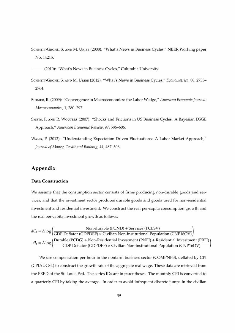
Schmitt-Groh´e, S. andM. Uribe (2008): “What’s News in Business Cycles,” NBER Working paper

No. 14215.

——— (2010): “What’s News in Business Cycles,” Columbia University.

Schmitt-Groh´e, S. andM. Uribe (2012): “What’s News in Business Cycles,” Econometrica, 80, 2733–

2764.

Shimer, R. (2009): “Convergence in Macroeconomics: the Labor Wedge,” American Economic Journal:

Macroeconomics, 1, 280–297.

Smets, F. and R. Wouters (2007): “Shocks and Frictions in US Business Cycles: A Bayesian DSGE

Approach,” American Economic Review, 97, 586–606.

Wang, P. (2012): “Understanding Expectation-Driven Fluctuations: A Labor-Market Approach,”

Journal of Money, Credit and Banking, 44, 487–506.

Appendix

Data Construction

We assume that the consumption sector consists of firms producing non-durable goods and ser-

vices, and that the investment sector produces durable goods and goods used for non-residential

investment and residential investment. We construct the real per-capita consumption growth and

the real per-capita investment growth as follows.

dC

t

= � log

Non-durable (PCND) + Services (PCESV)GDP Deflator (GDPDEF) ⇥ Civilian Non-institutional Population (CNP16OV)

!

dI

t

= � log

Durable (PCDG) +Non-Residential Investment (PNFI) + Residential Investment (PRFI)GDP Deflator (GDPDEF) ⇥ Civilian Non-institutional Population (CNP16OV)

!

We use compensation per hour in the nonfarm business sector (COMPNFB), deflated by CPI

(CPIAUCSL) to construct the growth rate of the aggregate real wage. These data are retrieved from

the FRED of the St. Louis Fed. The series IDs are in parentheses. The monthly CPI is converted to

a quarterly CPI by taking the average. In order to avoid infrequent discrete jumps in the civilian

39

noninstitutional population due to changes in population estimates, we use the HP trend instead.

The end-of-quarter observations are used to construct a quarterly population series.

For the sectoral labor, we use data on production and nonsupervisory employees from Table B-6

and the average weekly hours from Table B-7 of the Current Employment Statistics of the BLS.18 We

define the consumption sector as the union of non-durable and services industries and assume that

the investment sector consists of construction and durable firms. We simply construct the quarterly

total hours worked in each sector. We calculate the growth rate of average hours worked in each

sector by using the HP-trend population.

18Available at http://www.bls.gov/ces/cesbtabs.htm

40

inter-sectoral labor immobility, sectoral co-movement, and

Documents