inter-vehicle infrastructure

114 IEEE TRANSACTIONS ON VEHICULAR TECHNOLOGY, VOL. 40, NO. 1, FEBRUARY 1991

Automatic Vehicle Control Developments in the PATH Program

Steven E. Shladover, Charles A. Desoer, Fellow, ZEEE, J. Karl Hedrick, Masayoshi Tomizuka, Member, ZEEE, Jean Walrand, Senior Member, ZEEE, Wei-Bin Zhang, Donn H. McMahon,

Huei Peng, Shahab Sheikholeslam, Student Member, ZEEE, and Nick McKeown

Abstract-The accomplishments to date on the development of automatic vehicle control (AVC) technology in the Program on Advanced Technology for the Highway (PATH) at the University of California, Berkeley, are summarized. The basic prqfiiples and assumptions underlying the PATH work are identified, ‘followed by explanations of the work on automating vehicle lateral (steering) and longitudinal (spacing and speed) control. For both lateral and longitudinal control, the modeling of plant dynamics is described first, followed by development of the additional subsystems needed (communications, reference/sensor systems) and the derivation of the control laws. Plans for testing on vehicles in both near and long term are then discussed.

I. INTRODUCTION

HE California Program on Advanced Technology for the T Highway (PATH) has emphasized work on automatic vehicle control (AVC) technology to a greater extent than any of the other current IVHS programs. This emphasis has been decided upon for two different reasons. The primary reason for this emphasis is that AVC offers the most dramatic potential of any of the IVHS technologies for solving both traffic congestion and safety problems. Indeed, only AVC appears to be able to offer a roadway capacity increase that will compensate for more than one or two years of normal travel demand growth in California. The secondary reason for the emphasis on AVC is that it is most appropriate for a university research program to be emphasizing more advanced technologies than those currently being developed as products by private industry, rather than finding itself in potential competition with industry.

The PATH program is a collaboration between the Institute of Transportation Studies at the University of California at Berke- ley and the California Department of Transportation (Caltrans), with funding provided by Caltrans and the U.S. Department of Transportation. Private industry has been collaborating with PATH via cost-shared contracts and donations of equipment and services. In this govemment/academic/industrial partnership, the university is doing system engineering, exploratory research on new basic technologies, and evaluations of existing technologies. The private industry participants continue to do development of products, which is what they do best. The main thrust of the PATH program as such is not product development, however, but showing the technical feasibility of IVHS concepts so that decision makers will have a solid foundation of engineering

the research and development work progresses, this is likely to lead to public demonstrations of the most promising technologies.

Several basic assumptions underly the PATH vehicle control development work. It is important to review these assumptions up front, to set the context for the rest of the paper.

1) We are aiming for complete automation of the driving function on suitably equipped road facilities (most likely freeways, and initially on high-occupancy vehicle lanes), but not on all local roads and streets. This means that we are assuming the need for both lateral and longitudinal control of vehicles on these facilities. Partial automation (of either lateral or longitudinal, but not both) is not regarded as a desirable alternative because of potential human factors problems [l]. At this early stage in the PATH program, we have not attempted to integrate the lateral and longitudinal control functions, but have been seeking suitable approaches for each separately.

2) We are assuming that the most appropriate (cost-effective, technologically achievable) solutions will involve cooperation between the vehicle and the roadway, although we have not yet completed the system engineering studies needed to validate this assumption. As a consequence of this assumption, we are assuming that the roadways will be equipped with suitable reference “markers” and communication infrastructure, and that vehicles may also be equipped with cooperative devices (such as radar reflec- tors). We have therefore not adopted the concept of a fully autonomous vehicle that could travel under automatic control on any road or street.

3) Since the primary goal of the PATH program is develop- ing the technology to increase roadway capacity in order to alleviate congestion, we are not requiring adherence to the strict “brick wall” safety criterion for spacing between vehicles [l]. If we were to require “brick wall” stopping safety, capacity would actually be decreased relative to present-day freeway capacity because drivers are violating the brick wall criterion every day. The PATH approach, therefore, is not to design a system to have no rear-end collisions, but to design one in which the collisions that do inevitably occur have only minor effects.

data upon which to base future policy and funding deciiions. AS

Manuscript received August 1990. This work is a part of the Program on Advanced Technology for the Highway (PATH), prepared under sponsor- ship of the State of Califomia, Business Transportation and Housing Agency, Department of Transportation (Caltrans), and the U.S. Department of Trans- portation, Federal Highway Administration.

The authors are with the University of Califomia, Berkeley, CA 94720. IEEE Log Number 9040749.

safety will be the dominant factor in the design of any automatic vehicle control system. Clearly, major attention will have to be devoted to maximizing the reliability of d l elements of the system to minimize the probability of a failure Occurring.

the seriousness of those accidents that do occur. This has particular relevance for the selection of the nominal longitudinal spacing between vehicles on an automated roadway. If the

‘Omparable must be devoted to minimizing

oO18-9545/91/02oO-0114$01 .oO 0 1991 IEEE

-7

115 SHLADOVER et 01. : AUTOMATIC VEHICLE CONTROL DEVELOPMENTS IN THE PATH PROGRAM

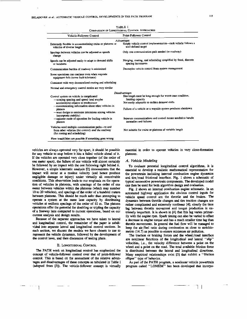
TABLE I COMPARISON OF LONGITUDINAL CONTROL APPROACHES

Vehicle-Follower Control Point-Follower Control

Advantages Extremely flexible in accommodating trains or platoons or

Spacings between vehicles can be adjusted as speeds

Speeds can be adjusted easily to adapt to demand shifts

Communication burden of roadway is minimized

Some operations can continue even when wayside

Consistent with very decentralized routing and scheduling

Normal and emergency control modes are very similar

Control system on vehicle is complicated

acceleration) relative to predecessor

platoon

(asymptotic stability)

platoon anomalies and failures

Simple vehicle control implementation--each vehicle follows a

Only one communication path needed (to roadway)

Merging, routing, and scheduling simplified by fixed, discrete

Decouples vehicle control from system management

vehicles of diverse length

change

or incidents spacing increments

well-defined target

equipment fails (some fault tolerance)

Disadvantages Slot length must be long enough for worst-case condition,

Not easily adaptable to sudden demand shifts

Failure of a vehicle or a wayside system produces shutdown

-sensing spacing and speed (and maybe

-communicating information about other vehicles in

-must design to minimize interations among vehicles

-separate mode of operation for leading vehicle in

Vehicles need multiple communication paths-to and from other vehicles (for control) and the roadway (for routing and scheduling)

Flow instabilities are possible if something goes wrong

limiting capacity

Separate communications and control means needed to handle

Not suitable for trains or platoons of variable length

vehicles are always operated very far apart, it should be possible for any vehicle to stop before it hits a failed vehicle ahead of it. If the vehicles are operated very close together (of the order of one meter apart), the failure of one vehicle will almost certainly be followed by an impact with the one following right behind it. However, a simple kinematic analysis [2] demonstrate8 that the impact will occur at a modest velocity (and hence produce negligible damage or injury) under virtually all conceivable conditions. This observation leads to our emphasis on the operation of vehicles in platoons, with spacings of the order of one meter between vehicles within the platoons (which may number 10 to 20 vehicles), and spacings of the order of a hundred meters between platoons. This should be much safer than attempting to operate a system at the same lane capacity by distributing vehicles at uniform spacings of the order of 10 m. The platoon operations offer the potential for doubling or tripling the capacity of a freeway lane compared to current operations, based on our current analysis and design results.

Because of the separate approaches we have taken to lateral and longitudinal control, the remainder of the paper is subdi- vided into separate lateral and longitudinal control sections. In each section, we discuss the models we have chosen to use to represent the vehicle dynamics, followed by the development of the control laws, and then discussion of testing plans.

II. LONGITUDINAL CONTROL The PATH work on longitudinal control has emphasized the

concept of vehiclefollower control over that of point-follower control. This is based on the assessment of the relative advantages and disadvantages of these concepts as tabulated in Table I (adopted from [3]). The vehicle-follower concept is virtually

essential in order to operate vehicles in very close-formation platoons.

A. Vehicle Modeling To evaluate potential longitudinal control algorithms, it is

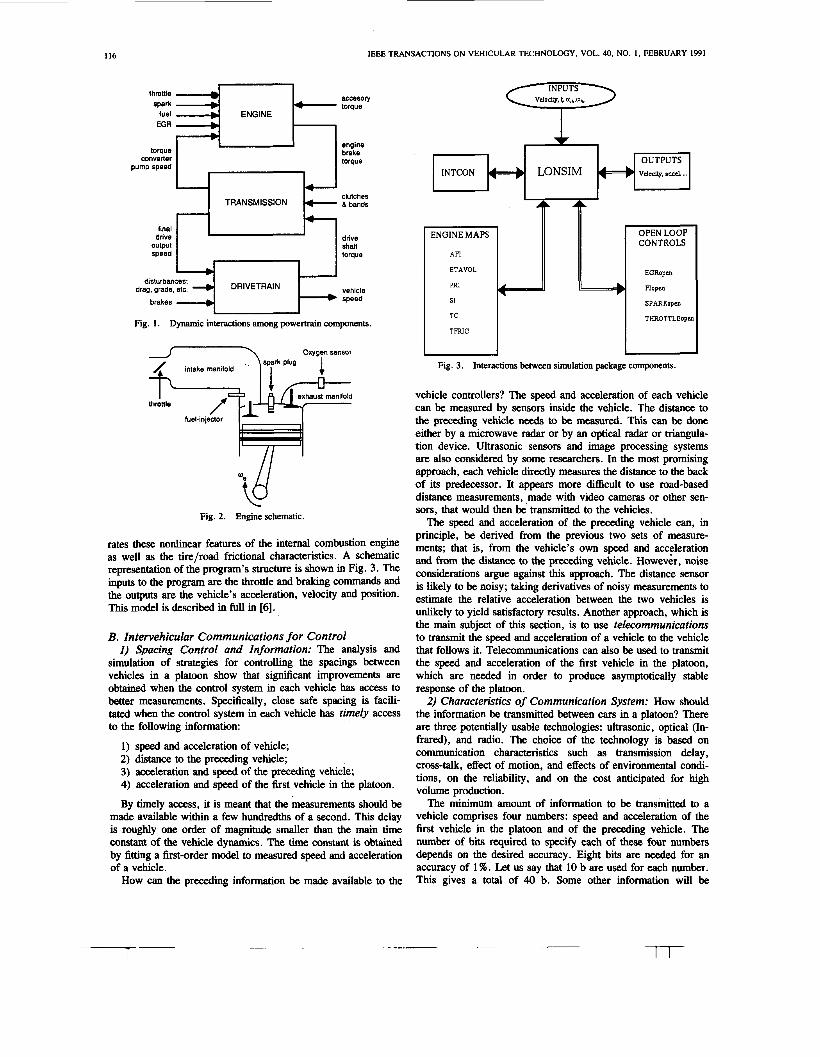
essential to develop a realistic mathematical representation for the powertrain including internal combustion engine dynamics and tire/road frictional interface. Fig. 1 shows a schematic of typical automotive powertrain components. The developed model can then be used for both algorithm design and evaluation.

Fig. 2 shows an internal combustion engine schematic. In an automated highway application the obvious control inputs for vehicle speed control are the throttle and the brakes. The dynamics between throttle changes and tire traction changes are rather complicated and extremely nonlinear [4]; clearly the time lag between throttle movement and torque production is extremely important. It is shown in [4] that this lag varies primar- ily with the engine rpm. Spark timing can also be varied to effect a decrease in engine torque and has a much smaller time lag than throttle movements. In general the fuel flow will be managed to keep the air/fuel ratio during combustion as close to stoichio- metric (14.7) as possible to ensure minimum air pollution.

The traction or braking forces and the wheel/road interface are nonlinear functions of the longitudinal and lateral “slip” velocities, i.e., the velocity difference between a point on the wheel and a point on the road. The total available friction force is distributed between the lateral and longitudinal directions. Many empirical relationships exist [5] that exhibit a “friction ellipse” type of behavior.

As part of the PATH program, a nonlinear vehicle powertrain program called “LONSIM” has been developed that incorpo-

I16 IEEE TRANSACTIONS ON VEHICULAR TECHNOLOGY, VOL. 40, NO. 1, FEBRUARY 1991

throttle accesory spark D 4 torque

fuel D ENGINE EGR D

engine torque brake

converter torque pump speed

clutches TRANSMISSION 8 bands

final 1 drive drive

output shaft speed toraue

vehicle speed

drag. grade. etc. DRIVETRAIN

brakes

Fig. 1. Dynamic interactions among powertrain components.

Oxygen sensoi

1 intake manifold

lhrdnie fuel-injector 41* 1

'7' Fig. 2. Engine schematic.

rates these nonlinear features of the intemal combustion engine as well as the tire/road frictional characteristics. A schematic representation of the program's structure is shown in Fig. 3. The inputs to the program are the throttle and braking commands and the outputs are the vehicle's acceleration, velocity and position. This model is described in full in [6].

B. Intervehicular Communications for Control I ) Spacing Control and Information: The analysis and

simulation of strategies for controlling the spacings between vehicles in a platoon show that significant improvements are obtained when the control system in each vehicle has access to better measurements. Specifically, close safe spacing is facili- tated when the control system in each vehicle has timely access to the following information:

1) speed and acceleration of vehicle; 2) distance to the preceding vehicle; 3) acceleration and speed of the preceding vehicle; 4) acceleration and speed of the first vehicle in the platoon.

By timely access, it is meant that the measurements should be made available within a few hundredths of a second. This delay is roughly one order of magnitude smaller than the main time constant of the vehicle dynamics. The time constant is obtained by fitting a first-order model to measured speed and acceleration of a vehicle.

How can the preceding information be made available to the

f

ENGINE MAPS

AFI

ETAVOL

PRI

SI

TC

TFRlC

L 1

+ CONTROLS

EGRnpen

Flopen

SPARKnpcn

THROTTLEopu

Fig. 3. Interactions between simulation package components.

vehicle controllers? The speed and acceleration of each vehicle can be measured by sensors inside the vehicle. The distance to the preceding vehicle needs to be measured. This can be done either by a microwave radar or by an optical radar or triangula- tion device. Ultrasonic sensors and image processing systems are also considered by some researchers. In the most promising approach, each vehicle directly measures the distance to the back of its predecessor. It appears more difficult to use road-based distance measurements, made with video cameras or other sensors, that would then be transmitted to the vehicles.

The speed and acceleration of the preceding vehicle can, in principle, be derived from the previous two sets of measurements; that is, from the vehicle's own speed and acceleration and from the distance to the precediig vehicle. However, noise considerations argue against this approach. The distance sensor is likely to be noisy; taking derivatives of noisy measurements to estimate the relative acceleration between the two vehicles is unlikely to yield satisfactory results. Another approach, which is the main subject of this section, is to use telecommunications to transmit the speed and acceleration of a vehicle to the vehicle that follows it. Telecommunications can also be used to transmit the speed and acceleration of the first vehicle in the platoon, which are needed in order to produce asymptotically stable response of the platoon.

2) Characteristics of Communication System: How should the information be transmitted between cars in a platoon? There are three potentially usable technologies: ultrasonic, optical (In- frared), and radio. The choice of the technology is based on communication characteristics such as transmission delay, cross-talk, effect of motion, and effects of environmental conditions, on the reliability, and on the cost anticipated for high volume production.

The minimum amount of information to be transmitted to a vehicle comprises four numbers: speed and acceleration of the first vehicle in the platoon and of the preceding vehicle. The number of bits required to specify each of these four numbers depends on the desired accuracy. Eight bits are needed for an accuracy of 1%. Let us say that 10 b are used for each number. This gives a total of 40 b. Some other information will be

SHLADOVER et al. : AUTOMATIC VEHICLE CONTROL DEVELOPMENTS IN THE PATH PROGRAM

-

117

exchanged to indicate that a vehicle is planning to leave the platoon or that it is facing some emergency condition. More- over, some error detection code will be added to the information. Let us assume that about 100 b have to be transmitted with a total delay less than about 0.01 s. The delay depends on the transmission rate, on the transmission errors, and on the communication protocol.

If the vehicles are connected by point-to-point error-free links, then the needed transmission rate is equal to 100 b divided by 0.01 s, i.e., 10000 b/s. This ideal situation is not imple- mentable. If we assume point-to-point links which transmit each packet correctly with probability 0.80, then a correct packet has a probability 0.99 of being correctly received after about three transmissions. With these assumptions, the required transmission rate is therefore about equal to 30000 b/s.

If the transmission proceeds from the first vehicle in the platoon to the other vehicles in a store-and-forward manner, by having each vehicle store the information that it receives from the vehicle preceding it and then retransmit it to the vehicle following it, then 14 transmissions are required before 100 b reach the last vehicle in a platoon of 15 vehicles. Assuming again a probability 0.80 of correct transmission and setting a goal of receiving the correct information within 0.01 s with probability at least 0.99, one can verify that the required transmission rate is about 230000 b/s. To see this, notice that the propagation of the information requires 14 successive correct transmissions of 100 b. This takes 14 + k attempts with probability

pk := 0.8 x (13; k)0.2*0.813,

which is the probability that 13 out of 13 + k attempts are correct and that the (14 + k)th attempt is also correct. We want to find the value of K so that po + p , + * - +pK = 0.99. Calculations give K = 9, which says that after a total of 14 + 9 = 23 transmission, the likelihood that the 100 b have been received correctly is about 0.99. Since it now takes 23 transmissions, the required rate is 23 times 100 b divided by 0.01 s, i.e., 230 000 b/s.

The above calculations neglect the processing time needed by a vehicle before it can retransmit the information. A custom design of the communication system can make that processing time negligible.

The next subsection discusses the physical implementation of the transmission.

3) Implementation of the Transmission: The calculations of the previous subsection indicate that an ultrasonic communication link is likely to be too slow for our application, since such a link typically operates at a rate less than 20000 b/s. As a consequence, two alternatives remain: radio waves or optical beams.

Conventional radio transmissions, at usual radio frequencies, are not very directional. One implication is that some procedure is required to identify the source of a received signal. Another implication is that different transmitters may end up competing for a common channel. The latter problem is referred to as the multiple access problem. A number of protocols have been designed for solving that problem. These multiple access protocols are suitable when each transmitter only needs the channel infrequently and at irregular times. In our application, the vehicle transmitters must transmit periodically, at regular times, and frequently.

The most efficient way of sharing a common channel under these conditions would be to implement a “round-robin” alloca- tion in which the transmitters take turns cyclically. For instance, in a platoon of 15 vehicles, the transmitters can take turns and the transmitter in the third vehicle gets to transmit every four- teenth transmission period. If three transmissions are required to be almost sure of a correct reception, we find that it takes 42 transmission periods before the third vehicle transmits its 50 bits of information to the fourth vehicle. This means that a transmission rate of 210 000 b/s is needed, assuming that the round-robin scheme can be implemented perfectly. In practice, the required protocol is rather complicated because the number of vehicles in a platoon changes frequently and because the synchronization of the transmissions requires a robust protocol. Another source of difficulty is the potential interference from neighboring vehicles that are not part of the same platoon. We believe that these difficulties can probably be resolved by using a code-hopping strategy which would use some information about the location of the vehicles to select the code to be used. Faced with the complexity of radio transmission for the

real-time control of vehicles in a platoon, we decided to consider an alternative approach based on infrared transmissions. An infrared communication link uses an optical transmitter, an optical receiver, and the associated electronics. The transmitter is a semiconductor laser diode (LD) or a light-emitting diode (LED). The transmitter converts an electrical signal into an infrared beam with a varying intensity. The receiver is either a p-i-n diode or an avalanche photo-diode (APD). The receiver produces an electrical signal which reflects the variations of the intensity of the infrared beam that it receives.

One advantage of an infrared communication link over radio is its directivity. By placing an optical transmitter in the back and a receiver in the front of each vehicle, each receiver knows that it is listening to the vehicle in front of it. This essentially eliminates the interference and the multiple access problems.

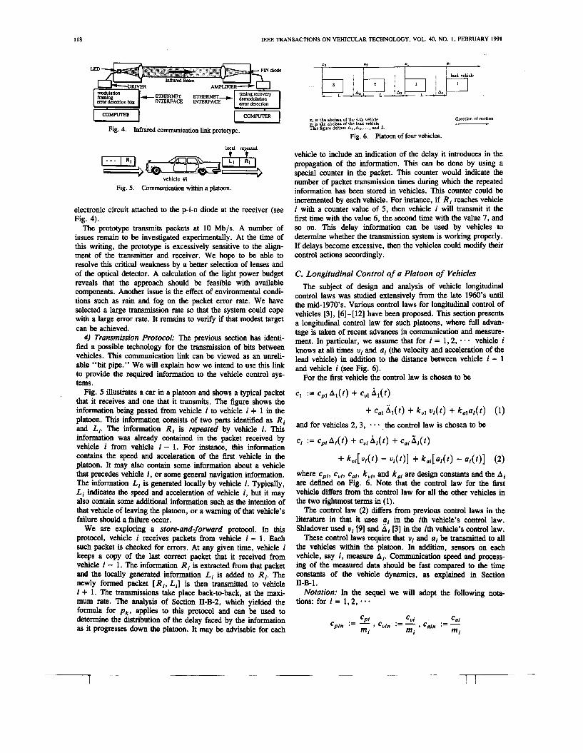
To determine the feasibility of such an optical communication link, one must identify suitable components and determine the characteristics of the transmission under typical operating conditions. We decided to construct a prototype to address those issues. Ultimately, the prototype will be tested on board vehicles. The design of that prototype is illustrated in the Fig. 4. The prototype is based on Ethernet interface boards. These boards, which are inserted into computers, convert a packet of 368-12000 b into a frame. A frame is the original packet preceded by a header and followed by a trailer. The header starts with a preamble and contains the addresses of the source and the destination computers and some control information. The preamble is used to synchronize the receiver. The trailer consists of error detection bits. The frame is then encoded by the Ethemet interface board into a Manchester code. The Manchester encoding of the bit 1 takes the value 0 during 50 ns (i.e., 50 x s)~followed by the value V for the same duration, where Y is a fixed voltage value. Similarly, the Manchester encoding of the bit 0 takes the value Y for 50 ns followed by the value 0 for the same duration. The bits follow one another every 100 ns, i.e., at the rate of 10 Mb/s. The Manchester encoding makes one transition during each bit transmission epoch. These transitions are used by the receiver to synchronize itself onto the received signal. In an Ethernet network, the Manchester-encoded frames are sent over a coaxial cable. In our prototype, the frames are sent to an electronic circuit, which turns an LED on whenever the Manchester signal takes the value V and turns it off when the signal takes the value 0. The frames are reproduced by an

11s IEEE TRANSACTIONS ON VEHICULAR TECHNOLOGY, VOL. 40, NO. 1 , FEBRUARY 1 9 9 1

ETHERNET ETHERNET- INERFACE INTERFACE

LED IN diode

Fig. 4. Infrared communication link prototype.

local rcDkllCd

vehicle #i Fig. 5. Communication within a platoon.

electronic circuit attached to the p-i-n diode at the receiver (see Fig. 4).

The prototype transmits packets at 10 Mb/s. A number of issues remain to be investigated experimentally. At the time of this writing, the prototype is excessively sensitive to the align- ment of the transmitter and receiver. We hope to be able to resolve this critical weakness by a better selection of lenses and of the optical detector. A calculation of the light power budget reveals that the approach should be feasible with available components. Another issue is the effect of environmental conditions such as rain and fog on the packet error rate. We have selected a large transmission rate so that the system could cope with a large error rate. It remains to verify if that modest target can be achieved.

4) Transmission Protocol: The previous section has identified a possible technology for the transmission of bits between vehicles. This communication link can be viewed as an unreli- able “bit pipe.” We will explain how we intend to use this link to provide the required information to the vehicle control systems.

Fig. 5 illustrates a car in a platoon and shows a typical packet that it receives and one that it transmits. The figure shows the information being passed from vehicle i to vehicle i + 1 in the platoon. This information consists of two parts identified as R i and Li. The information R i is repeated by vehicle i . This information was already contained in the packet received by vehicle i from vehicle i - 1. For instance, this information contains the speed and acceleration of the first vehicle in the platoon. It may also contain some information about a vehicle that precedes vehicle i , or some general navigation information. The information Li is generated locally by vehicle i . Typically, Li indicates the speed and acceleration of vehicle i , but it may also contain some additional information such as the intention of that vehicle of leaving the platoon, or a warning of that vehicle’s failure should a failure occur.

We are exploring a store-and-forward protocol. In this protocol, vehicle i receives packets from vehicle i - 1. Each such packet is checked for errors. At any given time, vehicle i keeps a copy of the last correct packet that it received from vehicle i - 1. The information R is extracted from that packet and the locally generated information Li is added to R i . The newly formed packet [ R,, Li] is then transmitted to vehicle i + 1. The transmissions take place back-to-back, at the maximum rate. The analysis of Section 11-B-2, which yielded the formula for Pk) applies to this protocol and can be used to determine the distribution of the delay faced by the information as it progresses down the platoon. It may be advisable for each

direction of motion :; ;: ;&& $:;E ;e& c

This figure defines AI, Az9. . . , and L.

Fig. 6. Platoon of four vehicles.

vehicle to include an indication of the delay it introduces in the propagation of the information. This can be done by using a special counter in the packet. This counter would indicate the number of packet transmission times during which the repeated information has been stored in vehicles. This counter could be incremented by each vehicle. For instance, if R i reaches vehicle i with a counter value of 5 , then vehicle i will transmit it the first time with the value 6, the second time with the value 7, and so on. This delay information can be used by vehicles to determine whether the transmission system is working properly. If delays become excessive, then the vehicles could modify their control actions accordingly.

C. Longitudinal Control of a Platoon of Vehicles The subject of design and analysis of vehicle longitudinal

control laws was studied extensively from the late 1960’s until the mid-1970’s. Various control laws for longitudinal control of vehicles [3], [6] - [ 121 have been proposed. This section presents a longitudinal control law for such platoons, where full advantage is taken of recent advances in communication and measurement. In particular, we assume that for i = 1,2, * * * vehicle i knows at all times uI and al (the velocity and acceleration of the lead vehicle) in addition to the distance between vehicle i - 1 and vehicle i (see Fig. 6).

c1 := cPl A l ( t ) + cV1 A , ( t )

For the first vehicle the control law is chosen to be

+ ca1 A l ( t ) + kvl U / ( t ) + koladt) (1)

and for vehicles 2,3, - the control law is chosen to be

ci := Cpi Ai( t ) + Cui Ai( t ) + cat A,( t )

where cpi, cui, cat, kvi , and kai are design constants and the A i are defined on Fig. 6. Note that the control law for the first vehicle differs from the control law for all the other vehicles in the two rightmost terms in (1).

The control law (2) differs from previous control laws in the literature in that it uses ar in the ith vehicle’s control law. Shladover used uI [9] and Ai [3] in the ith vehicle’s control law.

These control laws require that uI and aI be transmitted to all the vehicles within the platoon. In addition, sensors on each vehicle, say i , measure A i . Communication speed and processing of the measured data should be fast compared to the time constants of the vehicle dynamics, as explained in Section

Notation: In the sequel we will adopt the following nota- tions: for i = l , 2, * * - II-B- 1.

Cui c*i , Cuin := - , Cain := - CPi Cpin := - mi mi mi

I I9 SHLADOVER er al. : AUTOMATIC VEHICLE CONTROL DEVELOPMENTS IN THE PATH PROGRAM

kui kai k . :=- k . :=- mi mi

Kdi 2 Kdi

mi mi

urn 9 am

U0 9 dOi := - uo, d,i := -

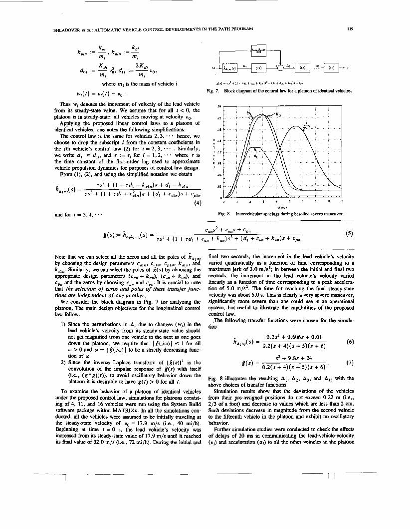
~(s) = rs3 t (1 t rd l + can + k..)s’ + (di + cun t k,)s + CP where m , is the mass of vehicle i Fig. 7. Block diagram of the control law for a platoon of identical vehicles. w , ( t ) : = U,(t) - uo.

Thus wl denotes the increment of velocity of the lead vehicle from its steady-state value. We assume that for all t < 0, the platoon is in steady-state: all vehicles moving at velocity uo.

Applying the proposed linear control laws to a platoon of identical vehicles, one notes the following simplifications:

The control law is the same for vehicles 2,3, - * * hence, we choose to drop the subscript i from the constant coefficients in the ith vehicle’s control law (2) for i = 2,3, - - - . Similarly, we write d , := d l l , and 7 := 7, for i = 1,2, where 7 is the time constant of the first-order lag used to approximate vehicle propulsion dynamics for purposes of control law design.

From (l), (2), and using the simplified notation we obtain

,24

f 1 .iz -

a -

A ,89 1 -

7s2 + ( 1 + 7dl - k a l n ) s + d , - kuln KA,w, ( s ) = 7s3 + (1 + 7dl + C & J S + (d , + C“& + C p l n

8 1 2 3 4 5 6 7 8 9

t(sec) (4)

and for i = 3,4, Fig. 8. Intervehicular spacings during baseline severe maneuver.

cans* + cuns + Cpn ’(‘):= j Z A i A i - l ( S ) = 7s3 + (1 + ~ d , + c,, + ka,)s2 + ( d , + c,, + kUn)s + cPn .

Note that we can select all the zeros and all the poles of AA,,,, by choosing the design parameters cain, cUlnr cpln, kaln, and kvln. Similarly, we can select the poles of d ( s ) by choosing the appropriate design parameters (can + k,,), (cun + k,,), and cpn and the zeros by choosing c,, and tun. It is crucial to note that the selection of zeros and poles of these transfer functions are independent of one another.

We consider the block diagram in Fig. 7 for analyzing the platoon. The main design objectives for the longitudinal control law follow.

1) Since the perturbations in Ai due to changes (w,) in the lead vehicle’s velocity from its steady-state value should not get magnified from one vehicle to the next as one goes down the platoon, we require that I d ( j w ) I 5 1 for all w > 0 and w + I &a) I to be a strictly decreasing function of a.

2) Since the inverse Laplace transform of [d(s)l2 is the convolution of the impulse response of d(s) with itself (i.e., ( g * g)( t ) ) , to avoid oscillatory behavior down the platoon it is desirable to have g ( t ) > 0 for all t .

To examine the behavior of a platoon of identical vehicles under the proposed control law, simulations for platoons consisting of 4, 11, and 16 vehicles were run using the System Build software package within MATRIXx. In all the simulations conducted, all the vehicles were assumed to be initially traveling at the steady-state velocity of uo = 17.9 m/s (i.e., 40 mi/h). Beginning at time t = 0 s, the lead vehicle’s velocity was increased from its steady-state value of 17.9 m/s until it reached its final value of 32.0 m/s (i.e., 72 mi/h). During the initial and

final two seconds, the increment in the lead vehicle’s velocity varied quadratically as a function of time corresponding to a maximum jerk of 3.0 m/s3; in between the initial and final two seconds, the increment in the lead vehicle’s velocity varied linearly as a function of time corresponding to a peak acceleration of 5.0 m/s2. The time for reaching the final steady-state velocity was about 5.0 s. This is clearly a very severe maneuver, significantly more severe than one could use in an operational system, but useful to illustrate the capabilities of the proposed control law.

,The following transfer functions were chosen for the simulation:

0.2s2 + 0.606s + 0.01 (6)

(7)

KA1w‘( s ) = 0.2(s + 4)(s + 5)(s + 6 )

s2 + 9.8s + 24 ’(‘) = 0.2(s + 4)(s + 5)(s + 6 ) .

Fig. 8 illustrates the resulting A, , A2, A3, and AIS with the above choices of transfer functions.

Simulation results show that the deviations of the vehicles from their pre-assigned positions do not exceed 0.22 m (i.e., 2/3 of a foot) and decrease to values which are less than 2 cm. Such deviations decrease in magnitude from the second vehicle to the fifteenth vehicle in the platoon and exhibit no oscillatory behavior.

Further simulation studies were conducted to check the effects of delays of 20 ms in communicating the lead-vehicle-velocity (U,) and acceleration (a , ) to all the other vehicles in the platoon


and of noisy measurement of A,. Simulation results for a platoon of ten vehicles show that the deviations in positions of all the vehicles from their respective preassigned positions are less than 0.29 m and decrease to values less than 2 cm. Note that the peak deviations decrease from the second vehicle to the tenth vehicle in the platoon and do not exhibit oscillatory behavior. This provides encouragement regarding the asymptotic stability of a platoon of arbitrary length.

We have shown that through the appropriate choice of design parameters, deviations in the successive vehicle spacings do not get magnified from the front to the back of a platoon of identical vehicles as a result of the lead vehicle’s acceleration from its initial steady-state velocity ( u o ) to its final steady-state velocity. Furthermore, the deviations in the successive vehicle spacings do not exhibit any oscillatory time-behavior and the magnitude of such deviations is well within one foot for a platoon of 16 vehicles.

In case the platoon consists of nonidentical vehicles, the displacement A, is affected not only by A,-], (as in the case above), but also to a small extent by A, - 2 , , A,. Recent work indicates that control laws inspired by (6) and (7) can be designed for a simple nonlinear vehicle model such that this interaction is eliminated [ 131.

D . Planned Experimental Veri3cation The modeling, design, and analysis of the vehicle-follower

control system described in the previous sections will be verified in a program of full-scale testing that has been initiated recently. The analyses and simulations have progressed as far as they can without benefit of such verification, which will be necessary to demonstrate that we can in fact accomplish what our models indicate.

The experimental program is being conducted on an eight-mile section of high-occupancy-vehicle (HOV) lanes in the median of Interstate 15 to the north of San Diego. This HOV facility contains two twelve-foot lanes, with ten-foot shoulders on both sides, separated from the rest of 1-15 by full Jersey barriers. These lanes are available for use by buses, vanpools and car- pools during the morning and afternoon rush hours, but are closed to the public for the rest of the day. Our experiments will be conducted when the facility is closed to the general public in order to ensure safety, and the air-bag-equipped vehicles will be driven by highly trained test drivers.

The experimental program is built around the use of a Doppler radar system developed by the Radar Control Systems Corpora- tion (RCS) of San Diego as an automotive collision warning device. The RCS radar provides measurements of the velocity difference between a vehicle and its predecessor and of the spacing between the vehicles. Each vehicle is equipped with 32-pole counters on the nondriven axles to provide accurate measurements of the vehicle’s own velocity. Acceleration is being estimated by differentiation of the velocity signals for the initial round of testing, but if this is found to be excessively noisy the vehicles will be equipped with accelerometers. The developers of the radar system expect it to produce accurate spacing (distance) measurements at spacings of the order of 10 m or more, but its shorter range performance is not yet assured. Therefore, even though we would hope to demonstrate vehicle- following performance at spacings of the order of 1 m to represent platoon operations, the minimum effective range in the test program is likely to be larger than that. Alternate sensing systems suitable for use at the shorter ranges are being evalu- ated, and if one is available before the end of the test program it

will be incorporated. Communication between vehicles will initially be implemented using a radio system, prior to the avail- ability of the infrared system described in Section II-B-3.

The test program begins with simple acceleration and deceler- ation tests to verify the longitudinal dynamics model of Section II-A. It continues with static characterizations of the radar sensor system performance under carefully controlled conditions, followed by basic vehicle following experiments with one automati- cally controlled vehicle following a manually driven vehicle. The culmination of the testing will be the operation of a platoon of four to six vehicles following a manually driven leader. Each vehicle in the test program will have a driver on board to provide steering control and to take over longitudinal control if necessary.

The ultimate outcome of the testing is expected to be an assessment of the feasibility of close-formation platoon operations and the development of performance specifications for the next generation of systems that will be needed.

III. LATERAL CONTROL The PATH lateral control work is focused on the concept of

cooperation between the vehicle and the roadway, with an intelligent vehicle receiving much of the information it needs from special elements installed in the roadway. This means that a lateral position reference is assumed to be installed in the road surface, and this reference is also expected to supply the vehicle with preview information about upcoming road geometry changes. This approach is thought to be considerably simpler and less expensive than the fully autonomous vehicle concept which relies on a vision system to “see” the existing lane edge striping.

The design of vehicle lateral controllers can be approached in two fundamentally different ways. The first is based on trying to reproduce human driver behavior [14], [15], and the second is based on application of control theory to vehicle dynamic models [ 161 - [ 191. We have adopted the latter approach.

A. Vehicle Lateral Dynamics Models Two dynamic models have been developed for the design and

analysis of the vehicle lateral controller. A six degree of freedom nonlinear model (complex model), is for representing the vehicle dynamics as realistically as possible, and a linearized model (simplified model) retains only the lateral and yaw dynamics. The former is utilized in the simulation study for evaluating the controller, and the latter in the design of the controller.

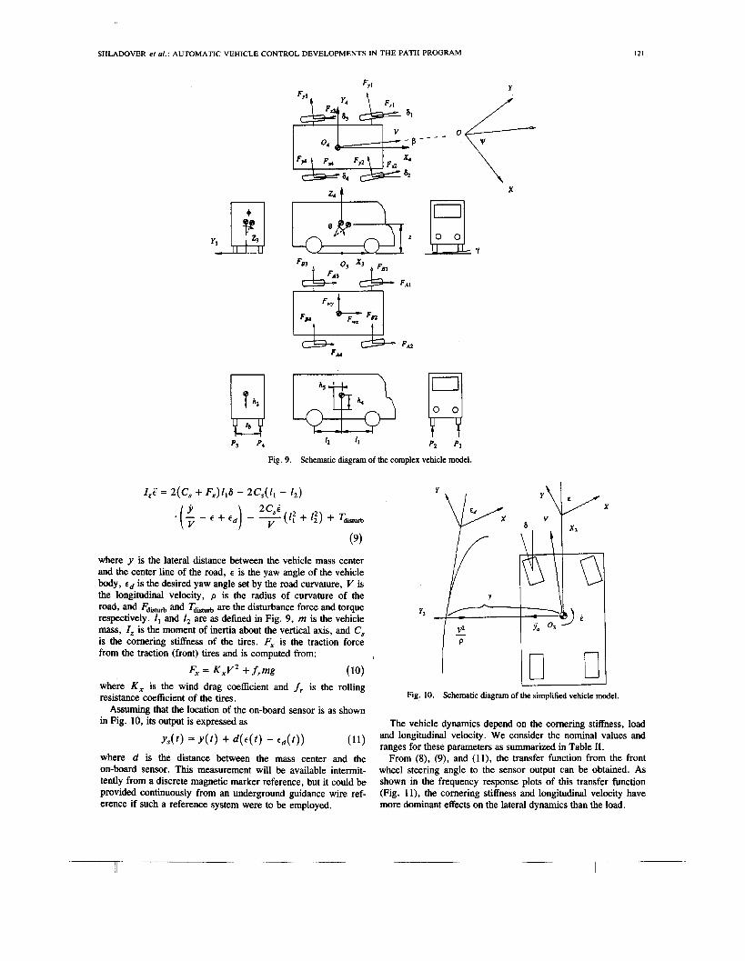
Complex Model: Fig. 9 shows the scope of the complex vehicle model. This model has the same level of complexity as the one developed by Lugner [20]. Vehicle body motion is described by 12 state variables: two each for the longitudinal, lateral, vertical, roll, pitch and yaw degrees of freedom. The angular velocities of the four tires are additional state variables. The input variables are the steering angle of each tire and traction forces, F, and Fy, acting on each tire. The traction forces are determined by a tire model which takes into consider- ation both the tire slip angle and slip ratio [21].

Simplified Model: The simplified model retains the lateral and yaw motions and is based on the following equations:

= 2 ( C , + F x ) 6 - - 4CsY + 4CS(€ - E d ) V

2CSi(I2 - I , ) + Fdishrrb V +

SHLADOVER et al. : AUTOMATIC VEHICLE CONTROL DEVELOPMENTS IN THE PATH PROGRAM 121

Fig. 9. Schematic diagram of the complex vehicle model.

ZzC = 2(Cs + F,)116 - 2C,(l, - 1,)

2 C,i . (; - E + €.) - ?( l f + 1;) + Tdisturb

(9)

where y is the lateral distance between the vehicle mass center and the center line of the road, E is the yaw angle of the vehicle body, E . is the desired yaw angle set by the road curvature, V is the longitudinal velocity, p is the radius of curvature of the road, and Fdisblrb and Tdshlrb are the disturbance force and torque respectively. I , and I , are as defined in Fig. 9, m is the vehicle mass, Z, is the moment of inertia about the vertical axis, and C, is the cornering stiffness of the tires. F, is the traction force from the traction (front) tires and is computed from:

F, = K,VZ + f,mg (10) where K , is the wind drag coefficient and f, is the rolling resistance coefficient of the tires.

Assuming that the location of the on-board sensor is as shown in Fig. 10, its output is expressed as

Y A t ) = Y O ) + d ( + ) - (11)

where d is the distance between the mass center and the on-board sensor. This measurement will be available intermit- tently from a discrete magnetic marker reference, but it could be provided continuously from an underground guidance wire reference if such a reference system were to be employed.

r X

V

Fig. 10. Schematic diagram of the simplified vehicle model.

The vehicle dynamics depend on the cornering stiffness, load and longitudinal velocity. We consider the nominal values and ranges for these parameters as summarized in Table 11.

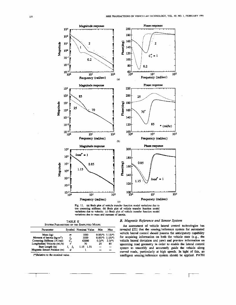
From (8), (9), and ( l l ) , the transfer function from the front wheel steering angle to the sensor output can be obtained. As shown in the frequency response plots of this transfer function (Fig. t l ) , the cornering stiffness and longitudinal velocity have more dominant effects on the lateral dynamics than the load.

B ~-

T I


Magnitude response

lo3 - 10' 102

109 100

Frequency (rdsec)

Magnitude response

lo3

103 100 10' 102

Frequency (rdsec)

100.- ; I #

80 - 0.2 , ,

10' 102 60' ' ' " " " ' ' ' ' s a a L l 100

Frequency (+l/sec)

Phase response

100 100 - 10' 102

Frequency (rad/sec)

Magnitude response 103

102

8 10' i!

E

.LI

$I 100

lo-' 10-2

10' 102 10.3 100

Frequency ( d s e c ) Frequency (rdsec)

Fig. 11. (a) Bode plot of vehicle transfer function model variations due to tire cornering stiffness. (b) Bode plot of vehicle transfer function model variations due to velocity. (c) Bode plot of vehicle transfer function model variations due to mass and moment of inertia.

(C)

TABLE II SYSTEM PARAMETERS OF THE SIMPLIFIED MODEL

Parameter Symbol NominalValue Min Max

Mass &@ m 1550 0.85(*) 1.15(*) Moment of hema &g-m*) I, 3100 0.85(*) 1.15(*)

Comering Stiffness (N/rad) C, 42000 0.2(*) 2.0(*) Longitudinal Velocity (mi/h) V 70 25 85

I , I2 1.15 1.51 - - - - "" LmLlth (m!

Magnctlc Sensor Posihon (m) d 1

(*)Relative to the nominal value.

B. Magnetic Reference and Sensor System An assessment of vehicle lateral control technologies has

revealed [22] that the sensing/reference system for automated vehicle lateral control should possess the anticipatory capability for acquiring information on both the vehicle state (e.g., the vehicle lateral deviation and yaw) and preview information on upcoming road geometry in order to enable the lateral control system to smoothly and accurately guide the vehicle along curved roads, particularly at high speeds. In light of this, an intelligent sensing/reference system should be applied. PATH

SHLADOVER et al. : AUTOMATIC VEHICLE CONTROL DEVELOPMENTS IN THE PATH PROGRAM 123

Road n o b

vehide I Dcviation I

I i r-----1 I L- I vehide I ,---A steering &- ,J 1 I , control ,

L - - - - - - J L-- - _ _ - J Fig. 12. System configuration.

studies indicate that approaches that might be used to acquire this information include 1) a “smart” vehicle-borne sensing system which would objectively “perceive” the road geometry and the vehicle state information-a direct (video) sensing approach, 2) a system which would utilize an “intelligent” reference system capable of conveying some of the aforementioned information to the vehicle-a coding and sensing approach, or 3) a combination of the above two schemes. We have decided that the coding and sensing approach ((2) above) has potential advantages and appears feasible for practical application on today’s roads. Fig. 12 illustrates the configuration of a system using this technique.

After a review of existing lateral control technologies, PATH has proposed to study an Intelligent Roadway Reference System (IRRS) using discrete magnetic markers. The concept incorporates the installation of very inexpensive permanent magnet markers in the center of the traffic lane. By alternating the polarity of the magnets, preview road information will be encoded. The permanent magnets offer the great advantage of being completely passive, which e l i t e s concerns about potential failures and greatly reduces maintenance requirements as well. The vehicle-borne sensing system acquires the pertinent information while passing over these markers, thus determining the vehicle deviation and road geometry that lies ahead. The lateral deviation measurements will allow the on-vehicle controller to give feedback commands in order to steer the vehicle back to the lane center, while the road geometry information will enable the controller to anticipate curvature changes. PATH experiments on the steering control of a scale model vehicle have shown that the anticipatory information is extremely important for a lateral control system using a discrete reference system.

In the PATH studies on the IRRS, techniques for lateral position sensing and processing have been researched intensively and approaches for road geometry information transmission and acquisition have been conceptually developed.

1) Information Processing for Vehicle Lateral Position Measurements: Magnetic sensing for lateral position measurements faces several interference problems, including: the over- lapping with the e d ’ s magnetic field, high frequency magnetic noise generated by the vehicle’s electrical system, and sponta- neous vertical movements of the vehicle. The problem with the earth’s field can be overcome by measuring the magnetic field of the markers (defined as the M-field) relative to the magnitude of the earth’s field. The vehicle magnetic noise can be reduced through a filtering process which incorporates a low-pass filter. Analysis shows that the vehicle vertical movements present the most critical issue. Studies have been conducted to develop an algorithm to overcome this problem.

Lateral position measurements, y , using the M-field can be

accomplished by constructing the relationship between the vehicle deviation and the magnetic field strength B, defined as

Efforts have been conducted to mathematically describe the M-field using the theory of magnetic fields, representing the M-field by its three components, B,, B y , and B,, written as

where B, and By are oriented tangent to and normal to the road center line respectively, while B, is perpendicular to the road surface. Analysis has been focusing on the M-field at x = 0, where only two nonzero components exist, defined as the horizontal component Bh(y, z) = By(O, y , z) and vertical component B,(y, z) = B,(O, y , z). Let s = B I ,=,-,, then the M-field strength at x = 0 is

and (15) can be rewritten as

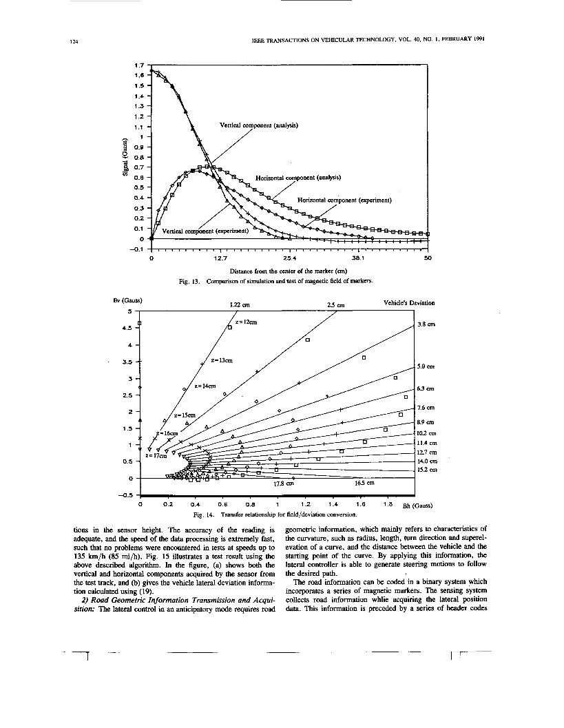
Fig. 13 gives both the test data and the analytical predictions of the magnetic field components. It was found that the analysis result has slight deviations from the test data. These deviations would cause errors if the vehicle position processing were dependent on (17). Furthermore, a study has shown that major simplifications should be introduced to derive a relationship between y and s, where y is specified not to relate to the height of the sensor, but the simplification could result in significant errors.

In order to derive (18), the properties of an input-output relationship of the function f are analyzed. A functional notation using set theory to specify f has been developed. Instead of investigating the function between the signal and vehicle’s deviation, this approach consists of a group of signal subsets which correspond to the digitized vehicle deviations { r i } . When a signal is acquired, the algorithm finds the subset to which it belongs and thereby identifies the vehicle’s deviation, thus the problem can be limited to the signal domain [23].

The definition of the signal subsets can be obtained from empirical data. Fig. 14 illustrates measurements of the two magnetic field components measured at various vehicle deviations and sensor heights. The regression of experimental data indicates that the relationship between B, and B, measured at a fixed vehicle deviation but at different heights has very good linearity. Therefore, a group of “deviation curves” { s i } (shown in Fig. 14) can be defined. The algorithm based on this approach consists of a set of rules { f i } and a lookup table, which covers the complete sensing range. The rule f i is written as:

f i : when B, = B,i, if i,i+l < B, C kUi thenyi+l < y < y i ( i + 1 , 2 ; . - , n ) . (19)

By applying these rules, the algorithm locates the vehicle’s deviation range. A more detailed estimate can be obtained by interpolation.

In field tests, a series of 2.5-cm diameter and 10-cm long ceramic magnetic bars were installed vertically in the center of the test track. Each magnetic bar provides a 25-cm radius M-field (measured at 12 cm above the road surface). Both simulations and full-scale tests demonstrated that the algorithm is able to reliably read the vehicle deviation independent of varia-


1.7

1.6

1 .5

1.4

1.3

1.2

1.1

- 1 3 0.9

2 0.8 1 0.7

0.6

0.5

0.4

0.3

0.2

0.1

0

.- v)

Vertical component (analysis) 1 \/ Horizontal component (experiment)

0 12.7 25.4 38.1

Distance from the Center of the marker (cm) . Comparison of simulation and Zest of magnetic field of markers. Fig. 13.

4.5 I 0 0.2 0.4 0.6 0.8 1 1.2 1.4 1.6 1.8 Bh (Gauss)

Fig. 14. Transfer relationship for field/deviation conversion.

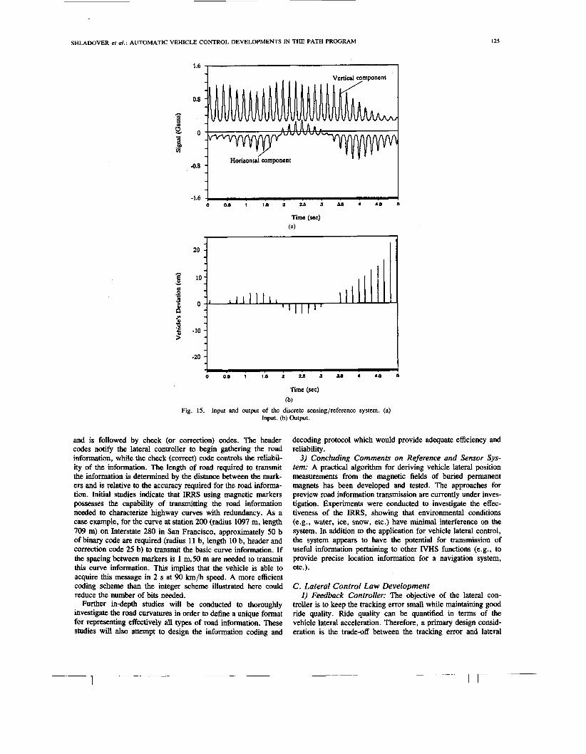
tions in the sensor height. The accuracy of the reading is adequate, and the speed of the data processing is extremely fast, such that no problems were encountered in tests at speeds up to 135 km/h (85 mi/h). Fig. 15 illustrates a test result using the above described algorithm. In the figure, (a) shows both the vertical and horizontal components acquired by the sensor from the test track, and (b) gives the vehicle lateral deviation information calculated using (19).

2) Road Geometric Information Transmission and Acqui- sition: The lateral control in an anticipatory mode requires road

geometric information, which mainly refers to characteristics of the curvature, such as radius, length, turn direction and superel- evation of a curve, and the distance between the vehicle and the starting point of the curve. By applying this information, the lateral controller is able to generate steering motions to follow the desired path.

The road information can be coded in a binary system which incorporates a series of magnetic markers. The sensing system collects road information whlie acquiring the lateral position data. This information is preceded by a series of header codes

T

SHLADOVER el al. : AUTOMATIC VEHICLE CONTROL DEVELOPMENTS IN THE PATH PROGRAM

20 -

3 10- Y

E P 1 0 - 1

I25

r l I I l l I l l I I I ”

1.6

Vertical component

0.8

n

3 .- 1 U - 0

v)

-0.8 I 1 1 ’

0.8

n

3 .- 1 U - 0

v)

-0.8

-1.6 4 0 0.6 1 Id 2 14 J 3.6 4 4.6 6

Time (sec) (a)

o 0.0 i (4 2 za J U 4 4 6 6

Time (sec) (b)

Fig. 15. Input and output of the discrete sensing/reference system. (a) Input. (b) Output.

and is followed by check (or correction) codes. The header codes notify the lateral controller to begin gathering the road information, while the check (correct) code controls the reliability of the information. The length of road required to transmit the information is determined by the distance between the markers and is relative to the accuracy required for the road information. Initial studies indicate that IRRS using magnetic markers possesses the capability of transmitting the road information needed to characterize highway curves with redundancy. As a case example,.for the curve at station 200 (radius 1097 m, length 709 m) on Interstate 280 in San Francisco, approximately 50 b of binary code are required (radius 11 b, length 10 b, header and correction code 25 b) to transmit the basic curve information. If the spacing between markers is 1 m,50 m are needed to transmit this curve information. This implies that the vehicle is able to acquire this message in 2 s at 90 km/h speed. A more efficient coding scheme than the integer scheme illustrated here could reduce the number of bits needed.

Further in-depth studies will be conducted to thoroughly investigate the road curvatures in order to define a unique format for representing effectively all types of road information. These studies will also attempt to design the information coding and

decoding protocol which would provide adequate efficiency and reliability,

3) Concluding Comments on Reference and Sensor Sys- tem: A practical algorithm for deriving vehicle lateral position measurements from the magnetic fields of buried permanent magnets has been developed and tested. The approaches for preview road information transmission are currently under investigation. Experiments were conducted to investigate the effectiveness of the IRRS, showing that environmental conditions (e.g., water, ice, snow, etc.) have minimal interference on the system. In addition to the application for vehicle lateral control, the system appears to have the potential for transmission of useful information pertaining to other IVHS functions (e.g., to provide precise location information for a navigation system, etc.).

C. Lateral Control Law Development I ) Feedback Controller: The objective of the lateral con-

troller is to keep the tracking error small while maintaining good ride quality. Ride quality can be quantified in terms of the vehicle lateral acceleration. Therefore, a primary design consid- eration is the trade-off between the tracking error and lateral

TI-


Qa

I I I I

1

Frequency (rWsec)

I 11 ' - k % La

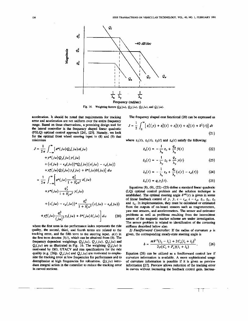
Fig. 16. Weighting factors Q J j w ) . Q,( j w ) , Q , ( j w ) , and Q.(b).

acceleration. It should be noted that requirements for tracking error and acceleration are not uniform over the entire frequency range. Based on these observations, a promising design tool for the lateral controller is the frequency shaped linear quadratic (FSLQ) optimal control approach [U], 1251. Namely, we look for the optimal front wheel steering input in (8) and (9) that minimizes

"L

where the first term in the performance index represents the ride quality, the second, third, and fourth terms are related to the tracking error, and the fifth term to the steering input. a( t ) in the first term denotes j i ( t ) , which can be obtained from (8). The frequency dependent weightings Q A j w ) , Q y ( j w ) , Q e ( j w ) and Q i ( j w ) are as illustrated in Fig. 16. The weighting Q A j w ) is motivated by ISO, UTACV and rms specifications for the ride quality (e.g. [26]). Q , ( j w ) and Q e ( j w ) are motivated to empha- size the tracking error at low frequencies for performance and to deemphasize at high frequencies for robustness. Q ; ( j o ) introduce integral action in the controller to reduce the tracking error in curved sections.

The frequency shaped cost functional (20) can be expressed as

J = -! Len[ z : ( y ) + z ; ( t ) + zg( f ) + z ; ( t ) + a 2 ( t ) ] dt 2

(21)

where z,(t), z2(t ) , ~ 3 ( t ) and z,(t) satisfy the following:

1 4 a i l ( t ) = - - z1 + - j q t )

All A,

1 4, AY AY

z&) = - - 2 2 + - y ( t )

1 4

A€ A, i 3 ( t ) = - - 2 3 + 2 ( ~ ( t ) - E d ( ? ) ) (24)

i4( t ) = qiYs( t ) * (25 ) Equations (8), (9), (22)-(25) define a standard linear quadratic

(LQ) optimal control problem and the solution technique is established. The optimal steering angle bop(?) is given in terms of linear feedback control of y, y , e - ed, i - id, zl, z2, z3 and 24. In implementation, they must be calculated or estimated from the outputs of on-board sensors such as magnetometers, yaw rate sensors, and accelerometers. The sensor and estimator problems as well as problems resulting from the intermittent nature of the magnetic marker scheme are under investigation. The sensor problem is related to identification of the cornering stiffness described below also.

2) Feedforward Controller: If the radius of curvature p is given, the corresponding steady-state steering angle is

Equation (26) can be utilized as a feedforward control law if curvature information is available. A more sophisticated usage of curvature information is possible if it is given as preview information [27]. Preview allows reduction of the tracking error in curves without increasing the feedback control gain. Increas-

SHLAWVER et al. : AUTOMATIC VEHICLE CONTROL DEVELOPMENTS IN THE PATH PROGRAM 121

ing feedback control gains to obtain accurate curve tracking at high speeds (or with substantial lateral [centrifugal] force) could introduce problems with ride quality or stability.

Estimation of the Cornering Stzflness: As pointed out in Section III-A, the vehicle lateral dynamics strongly depends on the cornering stiffness C, and the longitudinal velocity V . This indicates the need to schedule the FSLQ control gains as functions of the cornering stiffness and longitudinal velocity. While the velocity measurement from the speedometer is adequate for this purpose, the cornering stiffness must be estimated. The estimation scheme proposed in this paper is based on (8).

with the following relation utilized:

If all signals j j a , ya, E and C are measured or estimated, C, can be estimated by the least squares algorithm (e.g., 1281) to minimize

k J , (k ) = K k - i [ a m ( i ) - C , ( k ) b m ( i ) 1 2 (29)

i= 1

where K (0 < K < 1) is the forgetting factor, and

a , ( i ) = mjja(i)

are obtained froF signals measured at the kth sampling instant. The estimation C,(k) is computed from

r t - 1 1

L i = l J

4) Numerical Simulation: Fig. 17 shows the response of the overall controller consisting of the FSLQ feedback controller, the feedforward controller based on the curvature of road and the estimator for the cornering stiffness for the sample roadway illustrated in Fig. 18. Notice that the response is smooth, and the maximum error is within the sensor range. Simulations were repeated to confirm performance robustness of the overall system under a wide range of driving conditions such as a sudden wind gust, uneven tire pressures, and icy spots on the roadway. Simulation results showed acceptable performance for these off-nominal conditions [29].

D. Planned Experimental Veripcation As is the case with the longitudinal control development work,

we have advanced to the stage where we need experimental verification of the analyses and designs that have been developed thus far. We need to verify that the vehicle lateral dynamics are adequately represented by the two models we are using for control design and for simulation of control responses. We also need to verify that the control system works as modeled and simulated when it is operating in the presence of real-world noise, external forces, and imperfections in the placement of the reference markers and the road/tire coefficient of friction.

The experimental program begins with use of a scale-model automobile following reference magnets taped to the floor of an indoor conference room. This initial test vehicle is about 1-m long, 0.5-m wide, and weighs about 50 kg [30]. It is propelled by separate electric motors on each of its four wheels, each of which is steered by a separate motor. This makes the vehicle useful for experiments involving four-wheel steering as well as the more conventional two-wheel steering. The speed of the vehicle is controlled by a radio remote control unit, while its steering is controlled using the control logic developed here. Its on-board data acquisition system records the test results for subsequent reduction and analysis.

The second stage of the experimental program involves the use of a full-scale automobile which has been equipped with an electrically driven series servo steering control system. The reference information supplied by the magnetic markers buried beneath the surface of a roadway test section at the Richmond Field Station of the University of California at Berkeley is used to produce the control commands to the series servo. The driver of the test vehicle retains control by use of the steering wheel in the event the automatic system malfunctions in the tests. Subse- quent tests at higher speeds are expected to be conducted on other facilities where additional space makes the higher speeds feasible.

The experimental programs are expected to indicate how feasible the magnetic reference/sensor system is for lateral control and to show what performance improvements are possible with use of feedforward information about road geometry changes. Alternate reference/sensor systems are being studied in the PATH program to serve as backups for the magnetic system if it is found to have significant limitations in practice. The principal outcome of the testing is expected to be a determination of the feasibility of providing accurate lateral control using discrete, passive markers as the references.

IV. CONCLUSIONS AND RECOMMENDATIONS

This paper is clearly a report on work in progress, rather than a final report on results of a completed program. The PATH program has devoted its initial years to consolidating prior knowledge in the field of automatic vehicle control and develop- ing the analytical basis for moving forward with new developments. It is now entering the stage of testing its concepts to learn how well they work and to enhance those concepts with the benefit of test experience.

The technologies of automatic vehicle control are sufficiently challenging that we expect numerous iterations of design and testing to follow from the work we have initiated before the AVC systems are in the possession of everyday drivers. These iterations will involve the work of many professionals in both the public and private sectors, most of whom will not be university researchers. Many labor years of effort will be required to refine system designs, and especially to incorporate the needed safety and reliability capabilities. Substantial test facilities will also have to be developed to facilitate thorough testing of the systems at full scale before they are exposed to use by the general public. In the absence of such facilities, progress on these technologies will soon stall because we will have reached the limits of what we can learn using the presently available facilities.

Considering that the initial exploratory research on vehicle lateral and longitudinal control was conducted (and reported) more than 30 years ago, progress since then has been agoniz- ingly slow. Despite periods of activity in these fields in the

128 IEEE TRANSACTIONS ON VEHICULAR TECHNOLOGY, VOL. 40, NO. 1 , FEBRUARY 1991

450

400-

350

300-

250- .3 * 200-

130

100

50

0

1 0 10 20 30

time (sec)

-0.1 ‘

p = 630 m

turning 60’ -

- ~

-

2

1- I 0

-1 -

-2

I

0 10 20 30 time (sec)

0 10 20 30 time (sec)

-0.2

Fig. 17. Simulation result of nominal case.

1960’s and 1970’s, the total investment of resources was really quite modest. Now that the underlying technological base in computers, sensors, control theory and communications has advanced through many generations of progress and order of magnitude improvements in performance and cost effectiveness, the time should at long last be ripe for significant progress in automatic vehicle control.

REF E RE N c E s [l] S . E. Shladover and R. E. Parsons, “Safety issues for intelligent

vehicle/roadway systems,” presented at ASME Winter Ann. Meet., San Francisco, CA, in Engineering Applications of Risk Analysis, ASME, Dec. 1989.

121 S. E. Shladover, “Dynamic entrainment of automated guideway transit vehicles,” High Speed Ground Transport. J . , vol. 12, no. 3, pp. 87-113, Fall 1978.

[3] -, “Longitudinal control of automotive vehicles in close-formation platoons,” in Advanced Automotive Technologies- 1989, DSC-vol. 13, ASME Winter Annu. Meet., San Francisco, CA, Dec. 1989.

[4] D. Cho and J. K. Hedrick, “Automotive powertrain modelling for control,” J. Dynamic Syst., Measur. and Contr., vol. 111, Dec. 1989. E. Bakker, H. Pacejka, and L. Lidner, “A new tire model with an application in vehicle dynamics studies,” SAE paper no. 890087. D. H. McMahon, J. K. Hedrick, and S. E. Shladover, “Vehicle modeling and control for automated highway systems,” in Proc. 1990 Am. Contr. Conf., San Diego, CA, May 1990, pp.

L. L. Hoberock and R. J. Rouse, Jr., “Emergency control of vehicle platoons: System operation and platoon leader control,” J. Dynamic Syst., Meas. and Contr., vol. 98, no. 3, pp. 245-251, Sept. 1976.

[5]

[6]

297-303. [7]

i rr-

SHALDOVER et al. : AUTOMATIC VEHICLE CONTROL DEVELOPMENTS IN THE PATH PROGRAM 129

H. Y. Chiu, G. B. Stupp, Jr., and S. J. Brown, Jr., “Vehicle-follower control with variable gains for short headway automated guideway transit systems,” J . Dynamic Syst., Meas. and Contr., vol. 99, no. 3, pp. 183-189, Sept. 1977. S. E. Shladover, “Longitudinal control of automated guideway transit vehicles within platoons,” J . Dynamic Syst., Meas. and Contr., vol. 100, pp. 302-310, Dec. 1978. G. M. Takasaki, and R. E. Fenton, “On the identification of vehicle longitudinal dynamics,” IEEE Trans. Automat. Cont.,

A. S. Hauksdottir and R. E. Fenton, “On the design of a vehicle longitudinal controller,” IEEE Trans. Veh. Technol., vol. VT-

-, “On vehicular longitudinal controller design,” in Proc. 1988 IEEE Workshop Automotive Appl. of Electron., 1988,

S. Sheikholeslam and C. A. Desoer, “Longitudinal control of a platoon of vehicles,” in Proc. Am. Contr. Conf., San Diego, CA, May 1990, pp. 291-296. J. M. Carson and W. W. Wienville, “Development of a strategy model of the driver in lane keeping,” Veh. Syst. Dynamics,

R. W. Allen, H. T. Szostak, and R. J. Rosenthal, “Analysis and computer simulation of driver/vehicle interaction, ” SAE paper no. 871086, 1988. R. E. Fenton, G. C. Melocik, ahd K. W. Olson, “On the steering of automated vehicles: Theory and experiment,” IEEE Trans. Automat. Contr., vol. AC-21, June 1976. S. E. Shladover et al., “Steering controller design for automated guideway transit vehicles,” ASME J . D. Syst., Meas., Contr., vol. 100, Mar. 1978. H. Christ et al., “Automatic track control of vehicles: Theory and experiments,” Dynamics of Veh. on Roads and on Tracks, Proc. 5th VSD-2nd IUTAM Symp., Vienna, Sept. 1977, pp.

J. Ackermann and W. Sienel, “Robust control for automatic steering,” in Proc. I990 Am. Contr. Conf., San Diego, CA, May 1990, pp. 795-800. P. Lugner, “The influence of the structure of automotive models and tyre characteristics on the theoretical results of steady-state and transient vehicle performance,” in Dynamics of Veh. on Roads and on Tracks, Proc. 5th VSD-2nd [LITAM Symp., Vienna, Sept. 1977. H. Sakai, “Theoretical and experimental studies on the dynamical properties of tyres, Part 1: Review of theories of rubber friction,” Int. J . Veh. Design, vol. 2, no. 1, pp. 78-110, 1981. R. Parsons and W.-B. Zhang, “PATH lateral guidance system requirements definition,” in Proc. First Int. Conf. Appl. of Advanced Technol. in Transport. Eng., ASCE, San Diego, CA, Feb. 1989, pp. 275-280. Zhang et al., “An intelligent roadway reference system for vehicle lateral guidance/control,” in Proc. 1990 Am. Contr. Conf., San Diego, CA, May 1990, pp. 281-286. N. Gupta, “Frequency-shaped cost functionals: Extension of linear-quadratic-Gaussian design method,” J . Guidance and Contr., vol. 3, no. 6, pp. 529-535, Nov.-Dec. 1980. B. D. 0. Anderson and J. B. Moore, Optimal Control-Linear Quadratic Methods. Englewood Cliffs, NJ: Prentice-Hall, 1990. C. C. Smith, b. Y. McGhee, and A. J. Healey, “The prediction of passenger riding comfort from acceleration data,” ASME J . Dynamic Syst., Meas. and Contr., vol. 100, pp. 34-41, Mar. 1978. A. Y. Lee, “A preview steering autopilot control algorithm for four-wheel steering passenger vehicles,” Advanced Automotive Technol., 1989, pp. 83-98, ASME. K. J. Astrom and B. Wittenmark, Computer Controlled Sys- tems- Theory and Design. Englewood Cliffs, NJ: Prentice- Hall, 1990. H. Peng and M. Tomizuka, “Vehicle lateral control for highway automation,” in Proc. I990 Am. Contr. Conf., San Diego, CA, May 1990, pp. 788-794. M. Tomizuka and N. Matsumoto, “Vehicle lateral velocity and yaw control with two independent inputs,” in Proc. 1990 Am. Contr. Conf., San Diego, CA, May 1990, pp. 1868-1875.

vol. AC-22, pp. 610-615, Aug. 1977.

34, pp. 182-187, NOV. 1985.

pp. 77-83.

vol. 7, pp. 233-253, 1978.

145-164.

Steven E. Shladover received the S.B., S.M., and Sc.D. degrees in mechanical engineering from the Massachusetts Institute of Technology, Cambridge.

He conducted research on automated transportation systems at MIT. He spent 11 years working for Systems Control, Inc. and Systems Control Technology, Inc., Palo Alto, CA, before joining the Institute of Transportation Stud- ies at the University of California, Berkeley, in 1989, where he serves as the Technical Director

of the Program on Advanced Technology for the Highway (PATH). Dr. Shladover is a member of the American Society of Mechaincal

Engineers (ASME) where he currently serves as the Secretary of the Dynamic Systems and Control Division, a member of the Society of Automotive Engineers (SAE) and an Individual Affiliate of the Trans- portation Research Board (TRB). He is also a member of Tau Beta Pi, Pi Tau Sigma and Sigma Xi.

Charles A. Desoer (S’50-A’53- SM’57 - F’64) received the radio engineer degree from the University of Liege, Belgium, in 1949, the Sc.D. degree from the Massachusetts Institute of Technology, Cambridge, in 1953, and the Dr.Sc. @on. causa) from the University of Liege in 1976.

He worked at dell Telephone Laboratories, Murray Hill, NJ, from 1953-1958. Since 1958 he has been with the Department of Electrical Engineering and Computer Sciences, University

of California, Berkeley. From li)67-1%8 -he was with the Miller Institute, and from 1970-1971 he held a Guggenheim Fellowship. His interests lie in system theory with emphasis on control systems and circuits.

Dr. Desoer received the Best Paper Prize (with J. Wing) from JACC in 1962, the Medal of the University of Liege in 1970, the Distinguished Teaching Award from the University of California, Berkeley, in 1971, the 1975 IEEE Education Medal, and the Prix Montefiore in 1975. He also received the American Automatic Control Education Award in 1983 and the 1986 IEEE Control Systems Science and Engineering Award. He is a Fellow of AAAS and since 1977 a member of the National Academy of Engineering. One of his papers was one of three to receive an Honorable Mention from the IEEE Control Society in 1979. He is the author, with L. A. Zadeh, of Linear System Theory (1963); with E. S. Kuh, Basic Circuit Theory (1969); Notes for a Second Course on Linear Systems (1970); with M. Vidyasagar, Feedback Systems; Input-Output Properties (1975); with F. M. Callier, Multivariable Feedback Systems (1982); with L. 0. Chua and E. S. Kuh, Linear and Non-linear Circuits (McGraw-Hill, 1987).

J. Karl Heddck was with Arizona State Uni- versity, Tempe, from 1970- 1974, and a Profes- sor of Mechanical Engineering and Director of the Vehicle Dynamics Laboratory, Mas- sachusetts Institute of Technology, Cambridge, from 1974-1988. He is currently Professor of Mechanical Engineering at the University of California, Berkeley.

His research is concentrated on the application of dynamic modeling and control methods for ground vehicles including both rail and road

vehicles. Dr. Hedrick is currently a member of the Board of Directors of the

International Association of Vehicle System Dynamics (IAVSD), Editor of the Vehicle Systems Dynamic Journal, Associate Editor of the IEEE Control Systems Magazine, and Past Chairman of the ASME Dynamic Systems and Control Division.


Mdsayoshi Tomizuka (M’86) received the B.S. and M.S. degrees in mechanical engineering from Keio University, Tokyo, Japan, in 1968 and 1970, respectively, and the Ph.D. degree in mechanical engineering from the Massachusetts Institute of Technology, Cambridge, in 1974.

He is currently a Professor in and Vice Chairman of the Department of Mechanical En- gineering at the University of California, Berke- ley. His research interests include digital, optimal and adaptive control with applications to

mechanical systems such as vehicles, robotic manipulators and machine tools.

Dr. Tomizuka currently serves as the Technical Editor of the ASME Journal of Dynamic Systems, Measurement and Control.

Jean Walrand (S’71-M’74-SM’90) received the ingknieur civil degree in electrical engineering from the University of Likge, Belgium, in 1974, and the Ph.D. degree in electrical engineering from the University of California, Berkeley, in 1979.

From 1979 to 1981 he taught at Come11 University, Ithaca, NY, and since 1981 he has been with the Department of Electrical Engi- neering and Computer Sciences at the Univer- sity of California, Berkeley, where he is now

Professor. His research interests are in queueing networks, communication networks, stochastic control, stochastic simulation, and stochastic processes.

Dr. Walrand is the author of a number of technical papers in professional journals and of the textbook, An Introduction to Queue- ing Networks (Eng lewd Cliffs, NJ: Prentice-Hall, 1988). He has served as an Associate Editor for the IEEE TRANSACTIONS ON AUTO- MATIC CONTROL, and is on the editorial board of Systems and Control Letters, Queueing Systems, and Probability in the Engineering and Informational Sciences.

portation control syste

Wei-Bin Zhang received the B.S. and M.S. degrees in communications and control engineering from Northern Jiaotong University, Bei- jing, China, in 1982 and 1986 respectively.

He has been a Lecturer with the Communica- tion and Control Engineering Department of Northern Jiaotong University since 1982. Be- ginning in 1987, he has been a Visiting Assis- tant Research Engineer at the Institute of Trans- portation Studies, University of California at Berkeley. His research interests include trans-

:ms, system safety design and signal processing.

Donn H. McMahon received the S.B. degree from the Massachusetts Institute of Technology, Cambridge, in 1988 a d die M.S. degree from the University of California, Berkeley.

He is currently pursuing the Ph.D. degree at the University of California, Berkeley. His areas of interest are dynamics and control of nonlinear dynamical systems.

Huei Peng received the B.S. degree in mechanical engineering from National Taiwan Univer- sity, Taipei, Taiwan, in 1984, and the M.S. degree from Pennsylvania State University, Philadelphia, in 1988.

He is currently working toward the Ph.D. degree in mechanical engineering at the Univer- sity of California, Bbrkeley. His research interests include adaptive control and real-time control, with emphasis on vehicular systems.

networks. Mr . Sheikholeslam

Shahab Sheikholeslam (S’87) received the B.S. degree in computer engineering and the B.A. degree in mathematics from the University of California, Santa Cruz, in 1988, and the M.S. degree in electrical engineering from fhe Uni- versity of California, Berkeley, in 1989.

He is currently a Ph.D. candidate in the Department of Electrical Engineering and Com- puter Sciences at the University of California, Berkeley. His research interests are nonlinear control, vehicle dynamics, and communication

is a member of Phi Beta Kappa.

Nick McKeown was born in England. He received the undergraduate degree from the Uni- versity of Leeds, England, in 1986.

He is studying for the Ph.D. degree in the Department of Electrical Engineering and Com- puter Sciences at the University of California, Berkeley.

Mr. McKeown received, as an undergraduate, the National Engineering Scholarship from the Department of Engineering and Science; Undereraduate award for outstanding achieve-

ment, Leeds, 1986; Undergrazuate award for instrumentatiog and control, 1986; Institution of Electrical Engineer Undergraduate Scholarship for outstanding performance, 1985/1986.

inter-vehicle infrastructure

Documents