interaction between a cavitation bubble and …mae.eng.uci.edu/faculty/was/theme/pdfs/9.pdflayers,...
TRANSCRIPT
J. Fluid Mech. (2010), vol. 651, pp. 93–116. c© Cambridge University Press 2010
doi:10.1017/S0022112009994058
93
Interaction between a cavitation bubbleand shear flow
SADEGH DABIRI1, WILLIAM A. SIRIGNANO1†AND DANIEL D. JOSEPH1,2
1Department of Mechanical and Aerospace Engineering, University of California, Irvine, CA 92697, USA2Department of Aerospace Engineering and Mechanics, University of Minnesota, Minneapolis,
MN 55455, USA
(Received 24 July 2009; revised 14 December 2009; accepted 15 December 2009;
first published online 26 March 2010)
The deformation of a cavitation bubble in shear and extensional flows is studiednumerically. The Navier–Stokes equations are solved to observe the three-dimensionalbehaviour of the bubble as it grows and collapses. During the collapse phase of thebubble, two re-entrant jets are observed on two sides of the bubble. The re-entrantjets are not the result of interaction with a solid wall or free surface; rather, theyare formed due to interaction of the bubble with the background flow. Effects of theviscosity, surface tension and shear rate on the formation and strength of re-entrantjets are investigated. Re-entrant jets with enough strength break up the bubble intosmaller bubbles. Post-processing and analysis of the results are done to cast thedisturbance by the bubble on the liquid velocity field in terms of spherical harmonics.It is found that quadrupole moments are created in addition to the monopolesource.
1. IntroductionCavitation occurs in many applications, such as liquid injectors, propellers and
valves. Specifically, it is more common that cavitation inception occurs near or onsolid boundaries (Brennen 1995). This is due to the pressure drop caused by rapidchange in the flow direction. In addition, on these surfaces, inside the boundarylayers, high levels of shear stress are present, which may lead to a stress-inducedcavitation (Joseph 1998; Dabiri, Sirignano & Joseph 2007). In some cases, such asliquid injectors with sharp inlet corners, the boundary layer separates from the wallright behind the sharp corner. Therefore, it is of interest to study the interaction ofcavitation bubbles with a shear flow.
Dynamics of asymmetrical cavitation bubbles have been under investigation for along time. Most notably, cavitation bubbles near solid boundaries have been studiedby many researchers (Lauterborn & Bolle 1975; Blake & Gibson 1987). However,most of the numerical studies are limited to the boundary element method. Thisis mainly due to the advantage this method offers in reducing the dimensions ofthe problem by one. However, the drawback is that the method is limited to eitherirrotational flows or Stokes flows. Therefore, the case of a rotational flow at finiteReynolds number cannot be studied by this method.
† Email address for correspondence: [email protected]
94 S. Dabiri, W. A. Sirignano and D. D. Joseph
Navier–Stokes solutions of cavitation bubbles are very limited. Popinet & Zaleski(2002) studied the effects of viscosity on creation of re-entrant jets during collapseof a cavitation bubble near a rigid boundary. They have solved the Navier–Stokesequations in an axisymmetric problem and have showed that large viscosity preventsjet impact inside the bubble. Yu, Ceccio & Tryggvason (1995) also examined solutionsof Navier–Stokes equations for a bubble in viscous liquids. They considered thecollapse of a bubble in a shear flow near a rigid wall to simulate the condition ofcavitation bubbles inside a wall boundary layer. They found that, if the shear rate islarge enough, the creation of the re-entrant jets will be suppressed.
To study the deformation of bubbles in shear flow, a fundamental problem hasbeen considered here. A spherical bubble is placed initially in a simple shear flowand/or extensional flow; pressure drops for half a cycle and, in the next half cycle,recovers to its initial value. During this time, the bubble grows as it deforms due tostrain in the flow. Then, as the pressure recovers, the bubble collapses and rebounds.
In the next section, governing equations and numerical methods are explained.Then, a benchmark problem is presented to validate the code and finally, results ofthe bubble dynamics are presented and discussed.
2. Governing equationsWe consider the deformation of a cavitation bubble in a viscous liquid. The
governing equations for this three-dimensional problem follow:
ρi
(∂u∂t
+ u · ∇u)
= −∇p + ∇ · T + σκδ(d)n, (2.1)
where u, ρ and μ are the velocity, density and viscosity of the fluid, respectively.Subscript i could represent either liquid (l) or gas (g) phase and T is the viscous stresstensor. The last term represents the surface tension as a force concentrated on theinterface. Here, σ is the surface tension coefficient, κ is twice the local mean curvatureof the interface, δ is the Dirac delta function, d represents the distance from theinterface and n corresponds to the unit vector normal to the interface. The continuityequation for the liquid is
∇ · u = 0 (2.2)
and for the gas inside the bubble
∇ · u = − 1
ρ
Dρ
Dt. (2.3)
The bubble is assumed to consist of a non-condensable ideal gas going througha polytropic process, i.e. p ∝ ρn, where n is the polytropic exponent. For the smallbubbles and low frequencies of pressure variation, the process is closer to isothermalbecause the thermal diffusion time scale is smaller than the pressure variation timescale. On the other hand, for large bubbles and high frequencies, the process is closerto adiabatic. The value of n has been provided by Plesset & Prosperetti (1977) as afunction of two dimensionless parameters. For lower frequencies, which is the case inthis study, the value of n depends only on one of the parameters, G = R2
oω/Dg , whereω = 2π/T is the frequency and Dg is the thermal diffusivity of the gas. In this study,G =O(1) and therefore the process can be considered isothermal (n= 1). The density
Interaction between a cavitation bubble and shear flow 95
variation can be related to pressure variation as
1
ρ
Dρ
Dt=
1
np
Dp
Dt, (2.4)
where D/Dt represents the Lagrangian derivative. We consider the cases where thecollapse velocity of the bubble is much smaller than the speed of sound in the bubbleand the bubble density can be assumed to be uniform. The value of this uniformdensity, ρg , is related to the average pressure inside the bubble, pg , through thepolytropic equation, pg ∝ ρg
n. By relating the bubble density to the average pressureinside the bubble instead of the local pressure, one can suppress propagation ofacoustic waves inside the bubble. These waves occur on a time scale that is not ofinterest here. Therefore, the continuity equation for the gas phase is rewritten as
∇ · u = − 1
npg
dpg
dt(2.5)
inside the bubble.
3. Numerical implementationA finite-volume method on a staggered grid is used to discretize and find the
numerical solution of the unsteady Navier–Stokes equations. The convective andadvective terms are discretized using the QUICK scheme (Hayase, Humphrey &Greif 1992), and the SIMPLE algorithm, developed by Patankar (1980), is used tosolve the pressure–velocity coupling. The time integration is accomplished using thesecond-order Crank–Nicolson scheme.
A level-set method is used to capture the interface and model the surface tension,which has been developed by Osher and coworkers (e.g. Sussman et al. 1998 andOsher & Fedkiw 2001). The level-set function, denoted by θ , is defined as a signeddistance function. It has positive values in the gas phase and negative values in theliquid phase. The magnitude of the level set at each point in the computational fieldis equal to the distance from that point to the interface.
Time evolution of the level-set function is governed by
∂θ
∂t+ u · ∇θ = 0. (3.1)
Using the level-set function, one can define the fluid properties as
ρ = ρl + (ρg − ρl)Hε(θ), (3.2)
μ = μl + (μg − μl)Hε(θ), (3.3)
where subscripts l, g correspond to liquid and gas, respectively. Hε is a smoothedHeaviside function defined as
Hε =
⎧⎨⎩
0 θ < −ε,(θ + ε)/(2ε) + sin(πθ/ε)/(2π) |θ | � ε,1 θ > ε,
(3.4)
where ε represents the half-thickness of the interface, and has been given the valueof 1.5 times the grid spacing. Using the definition of the Heaviside function, one cancombine the continuity equations for liquid and gas phases (see (2.2) and (2.5)) into
96 S. Dabiri, W. A. Sirignano and D. D. Joseph
one equation:
∇ · u = − 1
npg
dpg
dtHε(θ). (3.5)
This single equation treats the gas inside the bubble as a compressible phase and theliquid as an incompressible phase.
4. Spherical cavitation bubbleIn order to check the accuracy of the code, a comparison is made with the solution
of spherical bubble growth and collapse. The radius of the bubble, R, is governed bythe Rayleigh–Plesset–Poritsky (RPP) equation (Plesset & Prosperetti 1977):
RR +3
2R2 =
1
ρl
{Pg − P∞ − 2σ
R− 4μl
RR
}, (4.1)
where P∞ is the pressure at infinity, and Pg is the pressure inside the bubble atthe interface and is related to the bubble volume through a polytropic equationPg = Po(Ro/R)3n, where Po is the pressure inside the bubble at the initial equilibriumradius, Ro. The bubble is initially at equilibrium and starts to grow, collapse andrebound as the pressure varies. The pressure variation is given by
P∞ =
{Po∞ − ΔP
2[1 − cos(2π t
T)] t < T ,
Po∞ T � t .(4.2)
Using the initial radius of the bubble, Ro, as the length scale and Ro
√ρl/Po∞ as the
time scale, one can derive the dimensionless form of the RPP equation as
R�R� +3
2R�2
=P �g − P �
∞ − 2
Wep
1
R�− 4
Rep
R�
R�, (4.3)
where Reynolds number, Weber number and dimensionless pressures are defined as
Rep =Ro
√ρlPo∞
μl
, Wep =RoPo∞
σ, P �
g =Pg
Po∞, P �
∞ =P∞
Po∞. (4.4)
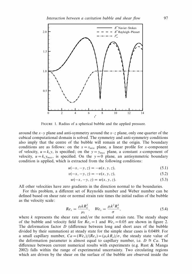
A three-dimensional calculation is performed, in which the centre of mass of thebubble is placed at the origin initially and stays there due to symmetry. Also, dueto spherical symmetry in the problem, only one eighth of the domain is solved on aCartesian grid with symmetrical boundary conditions on x–y, y–z and x–z planes. Onthe three other faces of the computational domain, time-varying pressure is applied.Since the boundaries of the domain are at finite distance, pressure from the solutionof the RPP equation is calculated at the position of the boundary and applied as thepressure boundary condition.
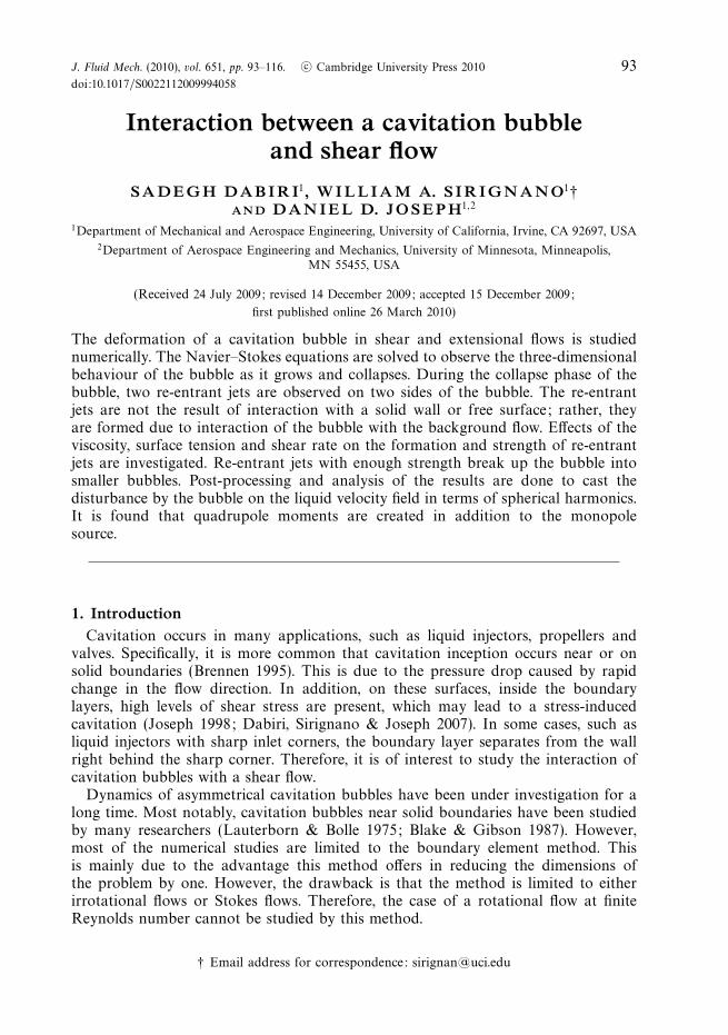
The computational domain consists of 503 grid points with 10 grids across theinitial radius of the bubble. Figure 1 shows the pressure variation and the resultingradius of the bubble predicted by the RPP equation and the Navier–Stokes solution.Dimensionless parameters are Rep = 70.71, Wep =500, (ΔP )/(Po∞) = 0.8, T � = 7.071.
5. Bubble in shear or extensional flows without pressure variationWe are interested in the interaction of the cavitation bubbles with a simple shear
flow. Therefore, we initially considered an incompressible bubble in a simple shearflow, u = ksy x. The bubble is placed at the centre of cubical domain. Due to symmetry
Interaction between a cavitation bubble and shear flow 97
t*0 2 4 6 8 10 12 14
0.5
1.0
1.5
2.0
R* Navier–Stokes
R* Rayleigh–Plesset
P*∞
Figure 1. Radius of a spherical bubble and the applied pressure.
around the x–y plane and anti-symmetry around the x–z plane, only one quarter of thecubical computational domain is solved. The symmetry and anti-symmetry conditionsalso imply that the centre of the bubble will remain at the origin. The boundaryconditions are as follows: on the x = xmin plane, a linear profile for x-componentof velocity, u = ksy, is specified; on the y = ymax plane, a constant x-component ofvelocity, u = ksymax , is specified. On the y = 0 plane, an antisymmetric boundarycondition is applied, which is extracted from the following conditions:
u(−x, −y, z) = −u(x, y, z), (5.1)
v(−x, −y, z) = −v(x, y, z), (5.2)
w(−x, −y, z) = w(x, y, z). (5.3)
All other velocities have zero gradients in the direction normal to the boundaries.For this problem, a different set of Reynolds number and Weber number can be
defined based on shear rate or normal strain rate times the initial radius of the bubbleas the velocity scale:
Res =ρlkR2
o
μl
, Wes =ρlk
2R3o
σ, (5.4)
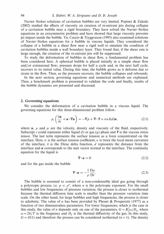
where k represents the shear rate and/or the normal strain rate. The steady shapeof the bubble and velocity field for Res = 1 and Wes =0.05 are shown in figure 2.The deformation factor D (difference between long and short axes of the bubbledivided by their summation) at steady state for the simple shear cases is 0.0489. Fora small capillary number, Ca = (Wes)/(Res) = (μlkRo)/σ , the steady state value ofthe deformation parameter is almost equal to capillary number, i.e. D ∼= Ca. Thedifference between current numerical results with experiments (e.g. Rust & Manga2002) falls within the range of experimental uncertainty. Two circulating regionswhich are driven by the shear on the surface of the bubble are observed inside the

98 S. Dabiri, W. A. Sirignano and D. D. Joseph
x
y
–1.5 –1.0 –0.5 0 0.5 1.0 1.5
x–1.5 –1.0 –0.5 0 0.5 1.0 1.5
–1.5
–1.0
–0.5
0
0.5
1.0
1.5
–1.5
–1.0
–0.5
0
0.5
1.0
1.5
x1 2
0
1
2
(a) (b) (c)
Figure 2. Steady shape of an incompressible bubble at Res =1. Wes =0.05 in (a) simpleshear flow, (b) normal-strain flow and (c) combined flow.
X
Y
(a) (b)
Shear flow schematic
X
Y
Extensional flow schematic
Figure 3. Schematics of shear and extensional flows. An initially spherical bubble is shownat the centre of the computational domain in addition to the far-field flow conditions.
bubble. These regions, which appear on top and bottom of the bubble, have the samevorticity direction as the simple shear flow.
Similar calculations are performed with normal strain and combined shear andnormal strains in the background flow. The strain rates are ks and kn and have thesame value as ks in the simple shear flow case. Results are shown in figure 2. Twosimilar recirculation regions formed in the simple shear flow are also present in thecases with combined shear and normal strain flows. In addition, two smaller regionsof recirculating flow can be seen inside the bubble on the left and right, which havevorticities opposite of the two larger vortices and the background flow.
6. Cavitation bubble with sinusoidal pressure variation interacting with shearor extensional flows
In this section, a cavitation bubble in simple shear flow, a normal strain flow or acombination of these flows is again considered. However, now the pressure will varywith time. A schematic of the problem is shown in figure 3. The bubble is initiallyspherical and is located at the origin. The initial velocity field is specified as u = ksy xfor shear flow, u = knx x − kny y for extensional flow or u = (ksy + knx)x − kny y for acombined shear and extensional flow. The boundary conditions for shear flow are thesame as explained in § 5, except that on x = xmin, a zero normal gradient is appliedinstead of applying a linear velocity profile. The reason for this change is that in the
Interaction between a cavitation bubble and shear flow 99
Case Res Wes Rep Wep k� T � ΔP � Flow type
1 0 0 70.71 500 0 7.071 0.8 Stagnant2 2.5 0.625 70.71 500 0.03535 7.071 0.8 Shear3 5.0 2.5 70.71 500 0.07071 7.071 0.8 Shear4 7.5 5.624 70.71 500 0.10606 7.071 0.8 Shear5 10.0 10.0 70.71 500 0.1414 7.071 0.8 Shear6 5 0.3535 70.71 25 0.07071 7.071 0.8 Shear7 1.0 0.05 14 9.8 0.07143 21 0.9796 Shear8 1.0 0.05 14 9.8 0.07143 21 0.9796 Normal strain9 1.0 0.05 14 9.8 0.07143 21 0.9796 Combined
10 4 0.2667 40 26.67 0.1 30 0.99 Shear
Table 1. List of parameters for cavitation bubble in strained flow.
case of the compressible bubble, the bubble volume will change with time. This willcreate a net out-flux or in-flux on the domain. To allow this flux to be distributedover all the surfaces of the computational domain, a Neumann boundary conditionis needed rather than a Dirichlet boundary condition. Dimensionless parameters arethe same as in § 4. In addition, the strain rate, k, either shear or normal, is providedin a dimensionless form as
k� = kRo
√ρl
Po∞. (6.1)
Table 1 shows a list of dimensionless parameters for the cavitation bubble and thetype of the background flow. Unlike the spherical cavitation bubble in stagnant flow(§ 4), where the pressure on boundaries can be calculated from the RPP equation, inthe strained flow, the pressure on the boundary cannot be calculated having only thevalue of pressure at infinity. Therefore, in this section, the pressure profile shown infigure 1 is applied directly on the boundary. To assess the effects of this change inthe boundary conditions, volume of the bubble is plotted for two cases in figure 4.The dashed line in figure 4(a) represents the case where the boundary condition forpressure is calculated from the RPP solution; this is, in fact, the same calculationas showed in § 4. The solid line represents the solution where the pressure is applieddirectly on the boundary (Case 1). Of course, there are differences between these twosolutions. Case 1 has a larger value of the maximum volume. Since, in this case,the pressure is applied on the boundary at a finite distance from the bubble, boththe pressure gradient outside the bubble and the rate of growth of the bubble willbe larger. Whereas, for the other case, the pressure variation is applied at infinityand the pressure value on the boundary is extracted from the solution of the RPPequation. The other difference is in the period of oscillation, which is smaller forCase 1. Similarly, this can be explained by considering the boundary conditions.Since the accelerated mass between the bubble surface and the boundary is smallerthan the accelerated mass between bubble surface and infinity, and the period ofoscillation increases with the mass, one should expect a larger period for Case 1compared to results of § 4. In another explanation, the boundary condition from theRPP equations results in a smaller pressure gradient over similar domains. This causesa smaller acceleration of liquid, and therefore, a longer period of oscillation for theRPP solution.
In figure 4(b), the volume of the bubble is shown for Cases 1–5. Note that for thesefive cases, all the parameters are the same and only the shear rate is changed. As it

100 S. Dabiri, W. A. Sirignano and D. D. Joseph
t*
Norm
aliz
ed v
olu
me
2 4 6 8 10 12 140
1
2
3
4
5
6
7
(a)
(b)
Norm
aliz
ed v
olu
me
0
1
2
3
4
5
6
7
BC on boundaryBC at infinity
t*2 4 6
Case 1Case 2Case 3Case 4Case 5
Figure 4. (a) Effect of boundary condition on volume of a spherical cavitation bubble in astagnant liquid; pressure variation applied directly on the boundary (solid line) and pressurevariation from the RPP solution (dashed line). (b) Effects of the shear on the bubble volume.
can be seen in figure 4, the shear rate has a negligible influence on the volume of thebubble. Still, it can be observed that the increase in the shear rate slightly suppressesthe growth of the bubble.
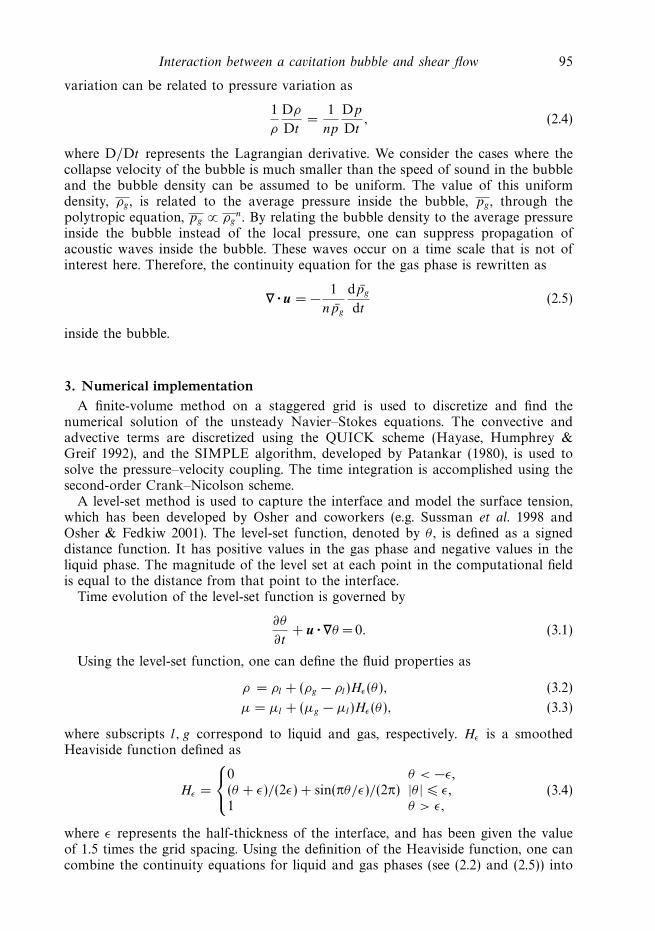
Figure 5 shows snapshots of the cavitation bubble from the instant it reaches itsmaximum volume until it collapses for Case 3. Figure 5(a) shows the bubble at itsmaximum volume. This maximum volume occurs slightly after the pressure reachesits minimum and starts to recover. This is due to the inertia of the liquid. At themaximum volume, the bubble has an ellipsoidal shape, which is a result of the shear

Interaction between a cavitation bubble and shear flow 101
0.2
0.4
0.3
x
y
–2 –1 0 1 2
x–2 –1 0 1 2
x–2 –1 0 1 2
x–2 –1 0 1 2
–2
–1
0
1
2
(a) (b)
(c) (d)
–2
–1
0
1
2
y
–2
–1
0
1
2
–2
–1
0
1
2
t/T = 0.75, t* = 5.303 (maximum volume)
1.01.4
1.2
1.1
0.9
1.3
t/T = 0.971, t* = 6.866
2.01.5
2.53.5
3.0
t/T = 1.001, t* = 7.078
15
10
5
t/T = 1.021, t* =7.220
Figure 5. Pressure contours and velocity field during collapse of cavitation bubble inshear flow for Case 3.
flow. As the bubble collapses, two regions of high pressure are formed on upperright and lower left sides of the bubble. These high pressure regions later lead tothe creation of two flat regions, and later concave regions, on the surface of thebubble. This finally results in the formation of two re-entrant jets on the sides of thebubble.
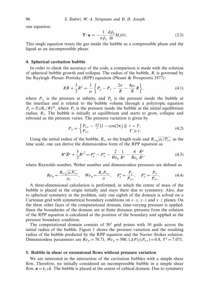
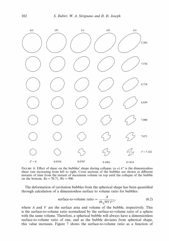
The shapes of the bubbles for Cases 1–5 are shown side by side in figure 6. Thelarge deformation of the bubbles can be explained by considering the Weber number.Since in these calculations the Weber number, Wep , is relatively large, the surfacetension is not strong enough to keep the bubble in a spherical shape.
As expected, the deformation of the bubble from a spherical shape at its maximumvolume is larger for cases with higher shear rate. Also, two re-entrant jets are formedon the two sides of the bubble.
102 S. Dabiri, W. A. Sirignano and D. D. Joseph
(a) (b) (c) (d) (e)
5.303
7.576
6.718
6.859
7.000
7.071
t* = 7.142
k* = 0 0.0354 0.0707 0.1061 0.1414
Figure 6. Effect of shear on the bubbles’ shape during collapse. (a–e) k� is the dimensionlessshear rate increasing from left to right. Cross sections of the bubbles are shown at differentinstants of time from the instant of maximum volume on top until the collapse of the bubbleon the bottom. Re = 70.71,We = 500.
The deformation of cavitation bubbles from the spherical shape has been quantifiedthrough calculation of a dimensionless surface to volume ratio for bubbles:
surface-to-volume ratio =A
(6√
πV )2/3, (6.2)
where A and V are the surface area and volume of the bubble, respectively. Thisis the surface-to-volume ratio normalized by the surface-to-volume ratio of a spherewith the same volume. Therefore, a spherical bubble will always have a dimensionlesssurface-to-volume ratio of one, and as the bubble deviates from spherical shape,this value increases. Figure 7 shows the surface-to-volume ratio as a function of
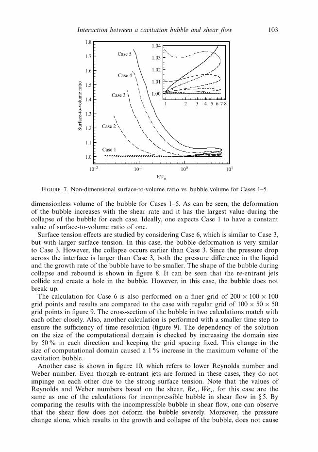
Interaction between a cavitation bubble and shear flow 103
V/Vo
Surf
ace-
to-v
olu
me
rati
o
10–2 10–1 100 101
1.0
1.1
1.2
1.3
1.4
1.5
1.6
1.7
1.8
Case 1
Case 2
Case 3
Case 4
Case 5
1 2 3 4 5 6 7 8
1.00
1.01
1.02
1.03
1.04
Figure 7. Non-dimensional surface-to-volume ratio vs. bubble volume for Cases 1–5.
dimensionless volume of the bubble for Cases 1–5. As can be seen, the deformationof the bubble increases with the shear rate and it has the largest value during thecollapse of the bubble for each case. Ideally, one expects Case 1 to have a constantvalue of surface-to-volume ratio of one.
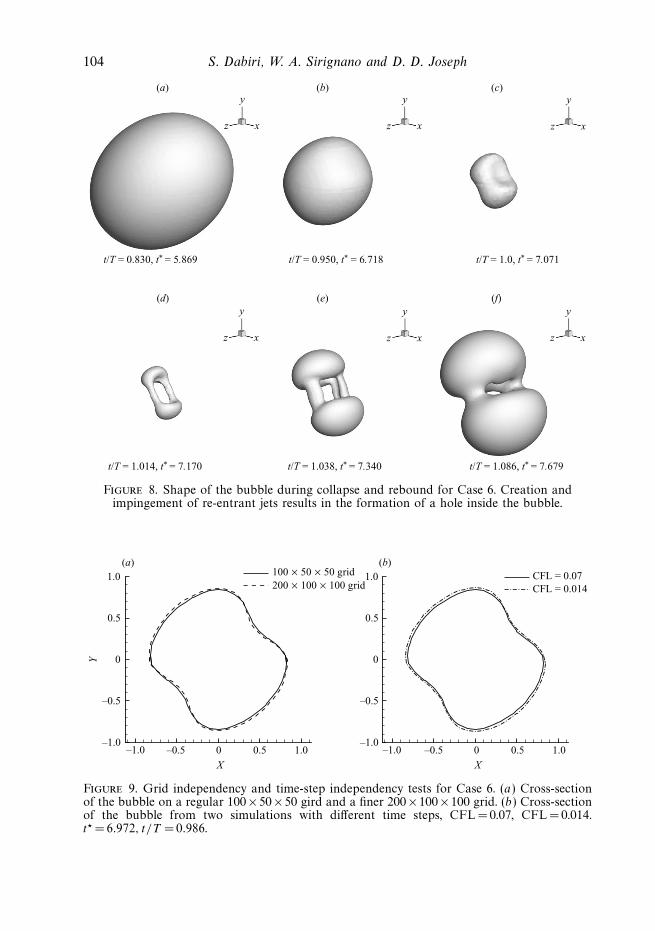
Surface tension effects are studied by considering Case 6, which is similar to Case 3,but with larger surface tension. In this case, the bubble deformation is very similarto Case 3. However, the collapse occurs earlier than Case 3. Since the pressure dropacross the interface is larger than Case 3, both the pressure difference in the liquidand the growth rate of the bubble have to be smaller. The shape of the bubble duringcollapse and rebound is shown in figure 8. It can be seen that the re-entrant jetscollide and create a hole in the bubble. However, in this case, the bubble does notbreak up.
The calculation for Case 6 is also performed on a finer grid of 200 × 100 × 100grid points and results are compared to the case with regular grid of 100 × 50 × 50grid points in figure 9. The cross-section of the bubble in two calculations match witheach other closely. Also, another calculation is performed with a smaller time step toensure the sufficiency of time resolution (figure 9). The dependency of the solutionon the size of the computational domain is checked by increasing the domain sizeby 50 % in each direction and keeping the grid spacing fixed. This change in thesize of computational domain caused a 1 % increase in the maximum volume of thecavitation bubble.
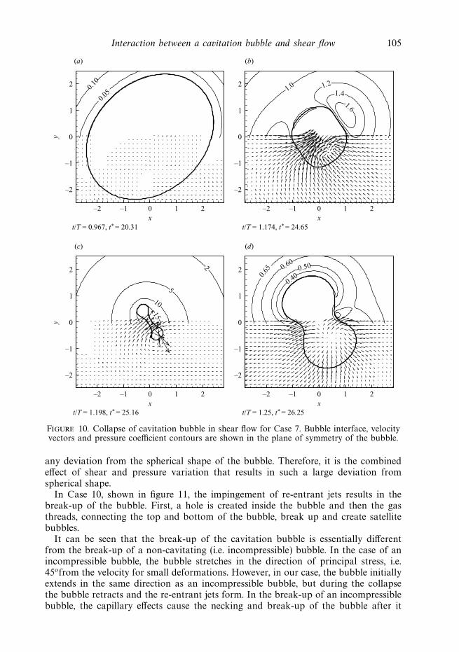
Another case is shown in figure 10, which refers to lower Reynolds number andWeber number. Even though re-entrant jets are formed in these cases, they do notimpinge on each other due to the strong surface tension. Note that the values ofReynolds and Weber numbers based on the shear, Res, Wes , for this case are thesame as one of the calculations for incompressible bubble in shear flow in § 5. Bycomparing the results with the incompressible bubble in shear flow, one can observethat the shear flow does not deform the bubble severely. Moreover, the pressurechange alone, which results in the growth and collapse of the bubble, does not cause
104 S. Dabiri, W. A. Sirignano and D. D. Joseph
t/T = 0.830, t* = 5.869 t/T = 0.950, t* = 6.718 t/T = 1.0, t* = 7.071
t/T = 1.014, t* = 7.170 t/T = 1.038, t* = 7.340 t/T = 1.086, t* = 7.679
y(a) (b) (c)
(d) (e) (f)
xz
y
xz
y
xz
y
xz
y
xz
y
xz
Figure 8. Shape of the bubble during collapse and rebound for Case 6. Creation andimpingement of re-entrant jets results in the formation of a hole inside the bubble.
X
Y
–1.0 –0.5 0 0.5 1.0–1.0
–0.5
0
0.5
1.0
(a) (b)
X
–1.0 –0.5 0 0.5 1.0–1.0
–0.5
0
0.5
1.0100 × 50 × 50 grid
200 × 100 × 100 gridCFL = 0.07
CFL = 0.014
Figure 9. Grid independency and time-step independency tests for Case 6. (a) Cross-sectionof the bubble on a regular 100×50×50 gird and a finer 200×100×100 grid. (b) Cross-sectionof the bubble from two simulations with different time steps, CFL= 0.07, CFL = 0.014.t� =6.972, t/T = 0.986.
Interaction between a cavitation bubble and shear flow 105
0.10
0.05
x
y
–2 –1 0 1 2
–2
–1
0
1
2
(a) (b)
(c) (d)
x–2 –1 0 1 2
–2
–1
0
1
2
x
y
–2 –1 0 1 2
–2
–1
0
1
2
x–2 –1 0 1 2
–2
–1
0
1
2
t/T = 0.967, t* = 20.31
1.2
1.4
1.6
1.0
t/T = 1.174, t* = 24.65
2
5
1015
t/T = 1.198, t* = 25.16
0.600.50
0.400.65
t/T = 1.25, t* = 26.25
Figure 10. Collapse of cavitation bubble in shear flow for Case 7. Bubble interface, velocityvectors and pressure coefficient contours are shown in the plane of symmetry of the bubble.
any deviation from the spherical shape of the bubble. Therefore, it is the combinedeffect of shear and pressure variation that results in such a large deviation fromspherical shape.
In Case 10, shown in figure 11, the impingement of re-entrant jets results in thebreak-up of the bubble. First, a hole is created inside the bubble and then the gasthreads, connecting the top and bottom of the bubble, break up and create satellitebubbles.
It can be seen that the break-up of the cavitation bubble is essentially differentfrom the break-up of a non-cavitating (i.e. incompressible) bubble. In the case of anincompressible bubble, the bubble stretches in the direction of principal stress, i.e.45ofrom the velocity for small deformations. However, in our case, the bubble initiallyextends in the same direction as an incompressible bubble, but during the collapsethe bubble retracts and the re-entrant jets form. In the break-up of an incompressiblebubble, the capillary effects cause the necking and break-up of the bubble after it

106 S. Dabiri, W. A. Sirignano and D. D. Joseph
xz
y
xz
y
xz
y
xz
y
xz
y
xz
y
(a) (b)
(c) (d)
(e) (f)
Figure 11. Shape of the bubble during collapse and rebound for Case 10. Creation andimpingement of re-entrant jets results in the break-up of the bubble. t∗ = 68.13 (a); 68.78 (b);68.95 (c); 69.03 (d); 69.07 (e); 69.16 (f ).
has been stretched by the shear in the flow. Whereas, here, the capillary phenomenondoes not play an important role in the break-up process. It is rather the inertia ofthe re-entrant jets that breaks up the bubble. Still one can say that the capillaryeffects become important in the break-up of the gas threads that are formed after there-entrant jets collide.
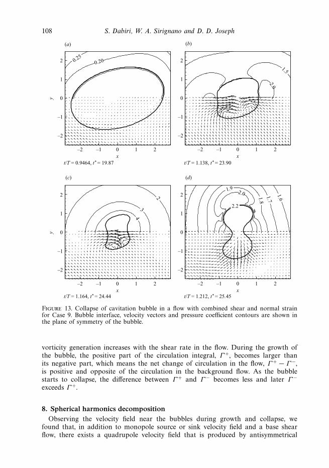
A case with a normal strain rate has also been considered. Figure 12 shows theshape of the bubble from the instance of its maximum volume until its collapse andrebound. This case has flow parameters similar to Case 7. However, the backgroundflow is extensional (u = kx x − ky y), with magnitude of the strain rate same as inCase 7. In this case, the bubble deforms during growth phase and elongates in thex direction. During the collapse of the bubble, a high pressure region is formedon the right (and left due to symmetry) side of the bubble and re-entrant jets areformed.
Case 9 has the combined shear and normal strain flow in the background.Figure 13 shows the shape of the bubble for this case. High pressure zones andre-entrant jets are still formed.
Interaction between a cavitation bubble and shear flow 107
0.1
x
y
0 1 2
x0 1 2
1
2
(a) (b)
(c) (d)
1
2
x
y
01 2
x
01 2
2
1
2
t/T = 0.967, t* = 20.31
1.0
0.8
0.7
t/T = 1.174, t* = 20.65
2.0
2.53.0
4.0
1.5
1.0
t/T = 1.198, t* = 25.16
1.0
0.91.11.2
t/T = 1.25, t* = 26.25
1
Figure 12. Collapse of cavitation bubble in a flow with normal strain for Case 8. Bubbleinterface, velocity vectors and pressure coefficient contours are shown in the plane of symmetryof the bubble.
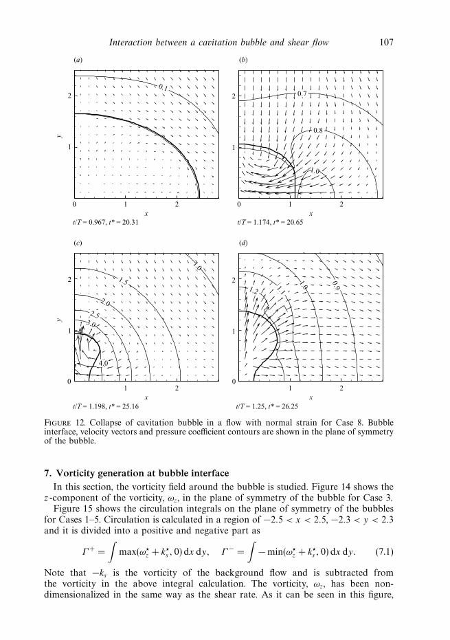
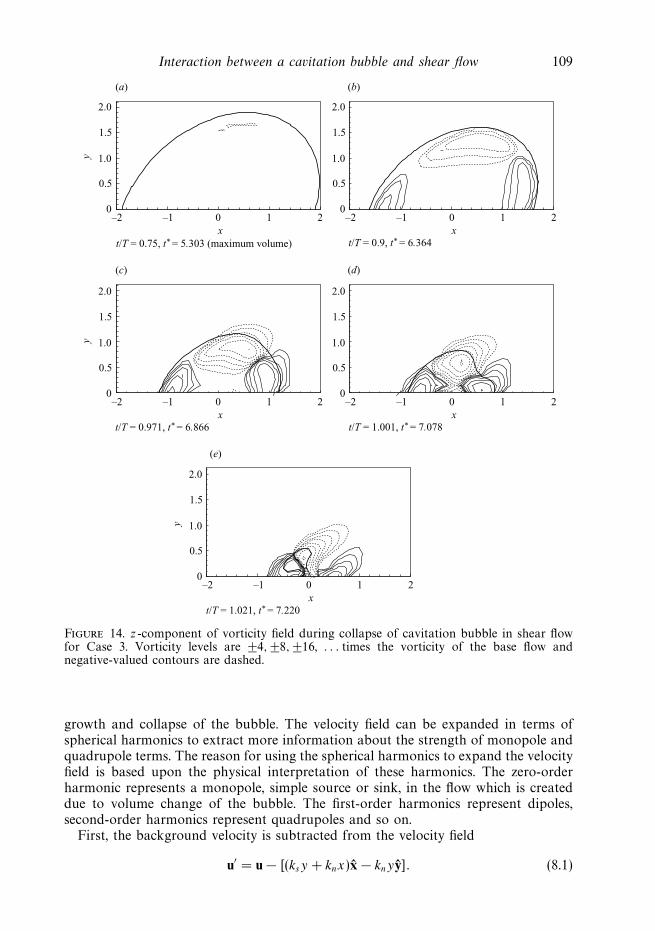
7. Vorticity generation at bubble interfaceIn this section, the vorticity field around the bubble is studied. Figure 14 shows the
z -component of the vorticity, ωz, in the plane of symmetry of the bubble for Case 3.Figure 15 shows the circulation integrals on the plane of symmetry of the bubbles
for Cases 1–5. Circulation is calculated in a region of −2.5 < x < 2.5, −2.3 < y < 2.3and it is divided into a positive and negative part as
Γ + =
∫max(ω�
z + k�s , 0) dx dy, Γ − =
∫− min(ω�
z + k�s , 0) dx dy. (7.1)
Note that −ks is the vorticity of the background flow and is subtracted fromthe vorticity in the above integral calculation. The vorticity, ωz, has been non-dimensionalized in the same way as the shear rate. As it can be seen in this figure,
108 S. Dabiri, W. A. Sirignano and D. D. Joseph
0.200.25
x
y
–2 –1 0 1 2
–2
–1
0
1
2
(a)
x–2 –1 0 1 2
–2
–1
0
1
2
x
y
–2 –1 0 1 2
–2
–1
0
1
2
x–2 –1 0 1 2
–2
–1
0
1
2
t/T = 0.9464, t* = 19.87
2.0
1.5
t/T = 1.138, t* = 23.90
4
3
2
t/T = 1.164, t* = 24.44
1.61.7
1.8
2.01.9
2.2
t/T = 1.212, t* = 25.45
(b)
(d)(c)
Figure 13. Collapse of cavitation bubble in a flow with combined shear and normal strainfor Case 9. Bubble interface, velocity vectors and pressure coefficient contours are shown inthe plane of symmetry of the bubble.
vorticity generation increases with the shear rate in the flow. During the growth ofthe bubble, the positive part of the circulation integral, Γ +, becomes larger thanits negative part, which means the net change of circulation in the flow, Γ + − Γ −,is positive and opposite of the circulation in the background flow. As the bubblestarts to collapse, the difference between Γ + and Γ − becomes less and later Γ −
exceeds Γ +.
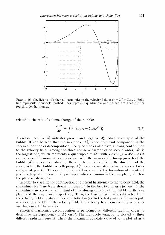
8. Spherical harmonics decompositionObserving the velocity field near the bubbles during growth and collapse, we
found that, in addition to monopole source or sink velocity field and a base shearflow, there exists a quadrupole velocity field that is produced by antisymmetrical
Interaction between a cavitation bubble and shear flow 109
x
y
–2 –1 0 1 20
0.5
1.0
1.5
2.0
x–2 –1 0 1 2
0
0.5
1.0
1.5
2.0
x
y
–2 –1 0 1 20
0.5
1.0
1.5
2.0
x
y
–2 –1 0 1 20
0.5
1.0
1.5
2.0
x–2 –1 0 1 2
0
0.5
1.0
1.5
2.0
t/T = 0.75, t* = 5.303 (maximum volume)
(a) (b)
(c)
(e)
(d)
t/T = 0.9, t* = 6.364
t/T = 0.971, t* = 6.866 t/T = 1.001, t* = 7.078
t/T = 1.021, t* = 7.220
Figure 14. z -component of vorticity field during collapse of cavitation bubble in shear flowfor Case 3. Vorticity levels are ±4, ±8, ±16, . . . times the vorticity of the base flow andnegative-valued contours are dashed.
growth and collapse of the bubble. The velocity field can be expanded in terms ofspherical harmonics to extract more information about the strength of monopole andquadrupole terms. The reason for using the spherical harmonics to expand the velocityfield is based upon the physical interpretation of these harmonics. The zero-orderharmonic represents a monopole, simple source or sink, in the flow which is createddue to volume change of the bubble. The first-order harmonics represent dipoles,second-order harmonics represent quadrupoles and so on.
First, the background velocity is subtracted from the velocity field
u′ = u − [(ksy + knx)x − knyy]. (8.1)
110 S. Dabiri, W. A. Sirignano and D. D. Joseph
t*
Γ+ ,
Γ−
0 2 4 6
2
4
6
8
10
1
2
3
4
5Γ +Γ −
Figure 15. Vorticity integrals or circulation on the plane of symmetry of the bubblesfor Cases 1–5.
Then, the radial component of the velocity field in spherical coordinates, with originat the centre of the bubble, is expanded:
u′r =
∑n,m
Amn (t, r)Y m
n (θ, φ), (8.2)
where Y mn ’s are the spherical harmonics, defined as
Y mn (θ, φ) =
√2n + 1
4π
(n − m)!
(n + m)!P m
n (cos θ)eimφ. (8.3)
Since we are dealing with real numbers for velocity field, the complex exponentialterm in the harmonics is replaced by its real and imaginary parts and some of thecoefficients are adjusted to make sure that the harmonics remain orthonormal.
Coefficients Amn in (8.2) can be found using
Amn (t, r) =
∫u′
rYmn (θ, φ) dΩ (8.4)
=
∫ π
θ=0
∫ 2π
φ=0
u′rY
mn (θ, φ) sin θ dθ dφ, (8.5)
where Amn is a function of r� and time; we will consider the time dependency of the
harmonics first. In a spherical coordinates with the origin placed at the centre ofthe bubble, the radial component of velocity is calculated at r� = 2. Then, the radialvelocity is expanded in spherical harmonics to find coefficients Am
n . Figure 16 showscoefficients of different harmonics as a function of time. Note that the first-orderharmonics, representing dipoles, are zero due to the symmetry and antisymmetryconditions in the problem. The dipole is zero because the bubble is not acceleratingrelative to the liquid. The zero-order harmonic represents a monopole and can be
Interaction between a cavitation bubble and shear flow 111
t*
0 1 2 3 4 5 6 7–6
–4
–2
0
2
A00
A0
A2c
A2s
A0
A2c
A2s
A4c
A4s
2
2
2
4
4
4
4
4
Figure 16. Coefficients of spherical harmonics in the velocity field at r� = 2 for Case 3. Solidline represents monopole, dashed lines represent quadrupole and dashed dot lines are forfourth-order harmonics.
related to the rate of volume change of the bubble:
dV �
dt �=
∫r�2
ur dA = 2√
πr�2A0
0. (8.6)
Therefore, positive A00 indicates growth and negative A0
0 indicates collapse of thebubble. It can be seen that the monopole, A0
0, is the dominant component in thespherical harmonics decomposition. The quadrupoles also have a strong contributionto the velocity field. Among the three non-zero harmonics of second order, A2s
2 isthe largest one, which represents a quadrupole at 45◦ with x -axis, (φ = 45◦). As itcan be seen, this moment correlates well with the monopole. During growth of thebubble, A2s
2 is positive indicating the stretch of the bubble in the direction of theshear. When the bubble is collapsing, A2s
2 becomes negative, which shows a fastercollapse at φ = 45◦. This can be interpreted as a sign of the formation of re-entrantjets. The largest component of quadrupole always remains in the x–y plane, which isthe plane of shear flow.
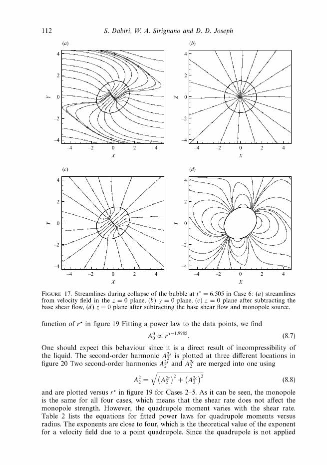
In order to visualize the contribution of different harmonics to the velocity field, thestreamlines for Case 6 are shown in figure 17. In the first two images (a) and (b) thestreamlines are shown at an instant of time during collapse of the bubble in the x–y
plane and the x–z plane, respectively. Then, the base shear flow is subtracted fromthe velocity field and streamlines are plotted in (c). In the last part (d), the monopoleis also subtracted from the velocity field. This velocity field consists of quadrupolesand higher-order harmonics.
Spherical harmonics decomposition is performed at different radii in order todetermine the dependency of Am
n on r�. The monopole term, A00 is plotted at three
different radii in figure 18. Then, the maximum absolute value of A00 is plotted as a
112 S. Dabiri, W. A. Sirignano and D. D. Joseph
X
Y
–4 –2 0 2 4
–4
–2
0
2
4
X
Z
–4 –2 0 2 4
–4
–2
0
2
4
X
Y
–4 –2 0 2 4
–4
–2
0
2
4
X
Y
–4 –2 0 2 4
–4
–2
0
2
4
(a) (b)
(c) (d)
Figure 17. Streamlines during collapse of the bubble at t∗ = 6.505 in Case 6: (a) streamlinesfrom velocity field in the z = 0 plane, (b) y = 0 plane, (c) z = 0 plane after subtracting thebase shear flow, (d ) z = 0 plane after subtracting the base shear flow and monopole source.
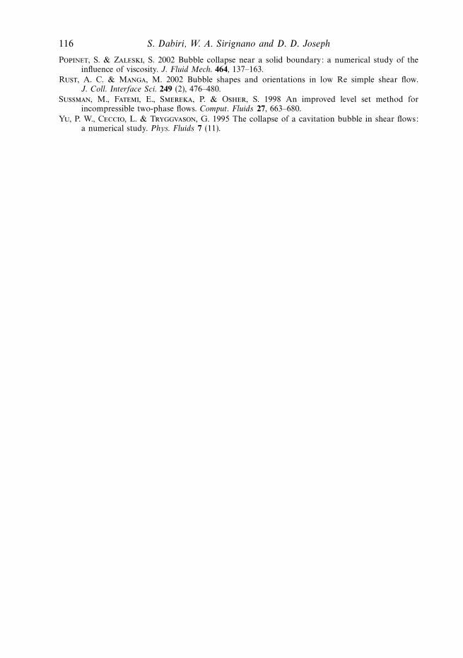
function of r� in figure 19 Fitting a power law to the data points, we find
A00 ∝ r�−1.9985
. (8.7)
One should expect this behaviour since it is a direct result of incompressibility ofthe liquid. The second-order harmonic A2s
2 is plotted at three different locations infigure 20 Two second-order harmonics A2s
2 and A2c2 are merged into one using
A22 =
√(A2s
2
)2+
(A2c
2
)2(8.8)
and are plotted versus r� in figure 19 for Cases 2–5. As it can be seen, the monopoleis the same for all four cases, which means that the shear rate does not affect themonopole strength. However, the quadrupole moment varies with the shear rate.Table 2 lists the equations for fitted power laws for quadrupole moments versusradius. The exponents are close to four, which is the theoretical value of the exponentfor a velocity field due to a point quadrupole. Since the quadrupole is not applied
Interaction between a cavitation bubble and shear flow 113
t*
A0
0 2 4 6–6
–4
–2
0
2
r = 2
r = 3
r = 4
0
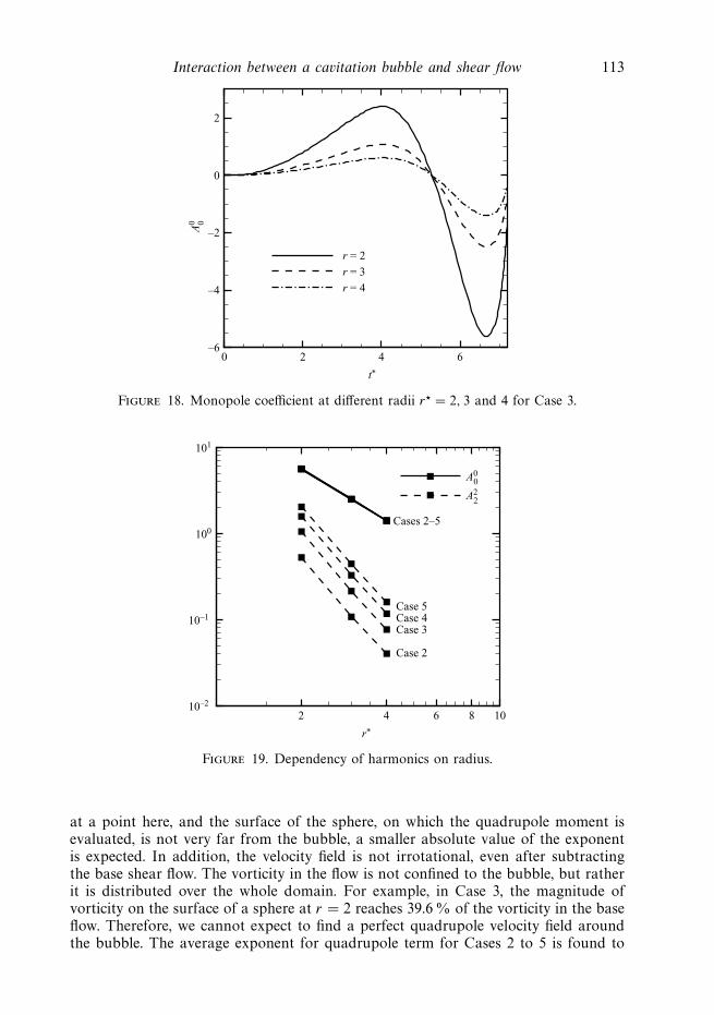
Figure 18. Monopole coefficient at different radii r� = 2, 3 and 4 for Case 3.
r*
2 4 6 8 1010–2
10–1
100
101
A0
A2
Case 5Case 4Case 3
Case 2
Cases 2–5
2
0
Figure 19. Dependency of harmonics on radius.
at a point here, and the surface of the sphere, on which the quadrupole moment isevaluated, is not very far from the bubble, a smaller absolute value of the exponentis expected. In addition, the velocity field is not irrotational, even after subtractingthe base shear flow. The vorticity in the flow is not confined to the bubble, but ratherit is distributed over the whole domain. For example, in Case 3, the magnitude ofvorticity on the surface of a sphere at r = 2 reaches 39.6 % of the vorticity in the baseflow. Therefore, we cannot expect to find a perfect quadrupole velocity field aroundthe bubble. The average exponent for quadrupole term for Cases 2 to 5 is found to

114 S. Dabiri, W. A. Sirignano and D. D. Joseph
t*
A2s
0 1 2 3 4 5 6 7
–1.0
–0.5
0
r = 2
r = 3
r = 4
2
Figure 20. Coefficients of second-order harmonics at different radii for Case 3.
k*
q2
0.02 0.04 0.06 0.08 0.10 0.12 0.140
5
10
15
20
25
30
2
Figure 21. q22 for different shear rates in the background flow.
be −3.736. Based on this average value, we define q22 as
A22 =
q22
r�−3.736. (8.9)
Hence, q22 is related to the quadrupole moment. Now, we can investigate the effect of
shear rate in the background flow on the quadrupole moment. Figure 21 shows thatthe quadrupole moment is proportional to the shear rate in the flow.

Interaction between a cavitation bubble and shear flow 115
Case A22
2 6.811r�−3.724
3 14.26r�−3.786
4 21.01r�−3.760
5 25.67r�−3.674
Table 2. Dependency of the quadrupole component of the velocity on r�.
9. ConclusionIn this paper, the deformation of a cavitation bubble due to the presence of a simple
shear and/or extensional flow is investigated. The general approach is to understandthe physics of the collapse of a cavitation bubble in shear flow. We are also interestedin learning the ways in which the cavitation bubble affects the flow. The creationof a monopole and three quadrupoles is one way of influencing the flow; anothermethod is by creating vorticity in the liquid phase. The deformation of the bubble inthe direction of the background flow during growth results in the creation of high-pressure regions on sides of the bubble during the collapse. This leads to formationof re-entrant jets as the bubble collapses. Impingement of re-entrant jets inside thebubble results in the break-up of the bubble in some cases. The deformation ofcavitation bubble with volume change is much larger than the incompressible bubblein the same flow environment. This suggests that the interaction between shear (ornormal strain) flow and volume change is very important and can strongly changethe behaviour of the cavitation bubble. A spherical harmonics decomposition of thevelocity field near the bubble shows formation of quadrupoles during the collapse ofthe bubble. The strength of the quadrupoles are proportional to the strain rate in thebackground flow.
This work was supported by the US Army Research Office through grant W911NF-06-1-0225 with Dr. Ralph A. Anthenien, Jr. as the scientific officer.
REFERENCES
Blake, J. R. & Gibson, D. C. 1987 Cavitation bubbles near boundaries. Annu. Rev. Fluid Mech. 19,99–123.
Brennen, C. E. 1995 Cavitation and Bubble Dynamics . Oxford University Press.
Dabiri, S., Sirignano, W. A. & Joseph, D. D. 2007 Cavitation in an orifice flow. Phys. Fluids 19 (7),072112.
Hayase, T., Humphrey, J. A. C. & Greif, R. 1992 A consistently formulated quick scheme for fastand stable convergence using finite-volume iterative calculation procedure. J. Comput. Phys.98, 108–118.
Joseph, D. D. 1998 Cavitation and the state of stress in a flowing liquid. J. Fluid Mech. 366, 367–376.
Lauterborn, W. & Bolle, H. 1975 Experimental investigations of cavitation-bubble collapse inneighbourhood of a solid boundary. J. Fluid Mech. 72, 391–399.
Osher, S. & Fedkiw, R. P. 2001 Level set methods: an overview and some recent results. J. Comput.Phys. 169, 436.
Patankar, S. V. 1980 Numerical Heat Transfer and Fluid Flow . Hemisphere.
Plesset, M. S. & Prosperetti, A. 1977 Bubble dynamics and cavitation. Annu. Rev. Fluid Mech. 9,145–185.
116 S. Dabiri, W. A. Sirignano and D. D. Joseph
Popinet, S. & Zaleski, S. 2002 Bubble collapse near a solid boundary: a numerical study of theinfluence of viscosity. J. Fluid Mech. 464, 137–163.
Rust, A. C. & Manga, M. 2002 Bubble shapes and orientations in low Re simple shear flow.J. Coll. Interface Sci. 249 (2), 476–480.
Sussman, M., Fatemi, E., Smereka, P. & Osher, S. 1998 An improved level set method forincompressible two-phase flows. Comput. Fluids 27, 663–680.
Yu, P. W., Ceccio, L. & Tryggvason, G. 1995 The collapse of a cavitation bubble in shear flows:a numerical study. Phys. Fluids 7 (11).