interaction. chd anger aspirin chd anger interaction = “effect modification”: the “effect”...
Post on 22-Dec-2015
224 views
TRANSCRIPT

Interaction


CHD
Anger
Aspirin
CHD
Anger
Interaction = “Effect modification”: The “effect” of the risk factor -- anger – on the outcome – CHD -- differs depending on the presence or absence of a third factor (effect modifier) --aspirin. The third factor (aspirin) modifies the effect of the risk factor (anger) on the outcome (CHD).
Note: to assess interaction, a minimum of 3 variables were needed in this study:•Aspirin•Anger•Coronary Heart Disease (CHD)
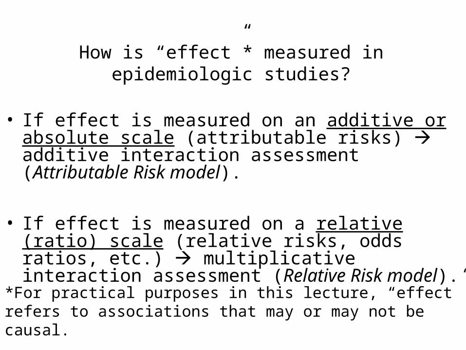
How is “effect”* measured in epidemiologic studies?
• If effect is measured on an additive or absolute scale (attributable risks) additive interaction assessment (Attributable Risk model).
• If effect is measured on a relative (ratio) scale (relative risks, odds ratios, etc.) multiplicative interaction assessment (Relative Risk model).
*For practical purposes in this lecture, “effect” refers to associations that may or may not be causal.

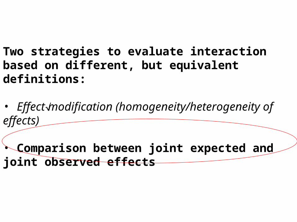
Two strategies to evaluate interaction based on different, but equivalent definitions:
• Effect modification (homogeneity/heterogeneity of effects)
• Comparison between joint expected and joint observed effects

First strategy to assess interaction:Effect Modification
ADDITIVE (attributable risk) interaction
Hypothetical example of absence of additive interaction
Z A Incidence rate (%) ARexp to A (%)
No No 10.0
Yes 20.0
Yes No 30.0
Yes 40.0
Potential effect modifier
Potential risk factor of primary interest

First strategy to assess interaction:Effect Modification
ADDITIVE (attributable risk) interaction
Hypothetical example of absence of additive interaction
Z A Incidence rate (%) ARexp to A (%)
No No 10.0
Yes 20.0
Yes No 30.0
Yes 40.0
Conclude: Because AR’s associated with A are not modified by exposure to Z, there is no additive interaction.
10.0
10.0

Hypothetical example of presence of additive interaction
Conclude: Because AR’s associated with A are modified by exposure to Z, additive interaction is present.
5.0
20.0
Z A Incidence rate (%) ARexp to A (%)
No No 5.0
Yes 10.0
Yes No 10.0
Yes 30.0
First strategy to assess interaction:Effect Modification
ADDITIVE (attributable risk) interaction

05
1015202530354045
A- A+
Inci
den
ce r
ate
(%)
Z+
Z-ARA
Example 1
Conclude:
-The stratum-specific effects (AR) are homogeneous
- Z does not modify the effect of A
-There is no (additive) interaction
0
5
10
15
20
25
30
35
A- A+
Inci
den
ce r
ate
(%)
Z+Z-
Example 2
Conclude:
-The stratum-specific effects (AR) are heterogeneous
- Z modifies the effect of A
-There is (additive) interaction
ARA
ARA
ARA
Ab
solu
te s
cale

Example of Effect Modification (Interaction) in a Clinical Trial with a Continuous Outcome
Average No. of New Nevi
Freckles, % Sunscreen Control Difference
10 24 24 0
20 20 28 -8
30 20 30 -10
40 16 30 -14
From: Szklo, Arch Dermatol 2000;136:1546 (Based on Gallagher et al, 2000)

3530
25
20
15
10
5
0
5 10 20 30 40Freckles, %
New
Nev
i, N
o.
Example of Freckling as an Interacting Variable (Effect Modifier)
Sunscreen Control
Sunscr << ContSunscr < Cont
From: Szklo, Arch Dermatol 2000;136:1546 (Based on Gallagher et al, 2000)

Hypothetical example of absence of multiplicative interaction
Z A Incidence rate (%) RRA
No No 10.0
Yes 20.0
Yes No 25.0
Yes 50.0
Conclude: Because RR’s associated with A are not modified by exposure to Z, there is no multiplicative interaction.
2.0
2.0
First strategy to assess interaction:Effect Modification
MULTIPLICATIVE (ratio-based) interaction

Hypothetical example of presence of multiplicative interaction
Z A Incidence rate (%) RRA
No No 10.0
Yes 20.0
Yes No 25.0
Yes 125.0
Conclude: Because RR’s associated with A are modified by exposure to Z, multiplicative interaction is present.
2.0
5.0
First strategy to assess interaction:Effect Modification
MULTIPLICATIVE (ratio-based) interaction

0
20
40
60
80
100
120
140
A- A+
Inci
den
ce r
ate
(%)
Z+Z-
Example 1
0
20
40
60
80
100
120
140
A- A+
Inci
den
ce r
ate
(%)
Z+
Z-
Example 2
Is this the best way to display the data?
NO!
1
10
100
1000
A- A+
Inci
den
ce r
ate
(%)
Z+
Z-
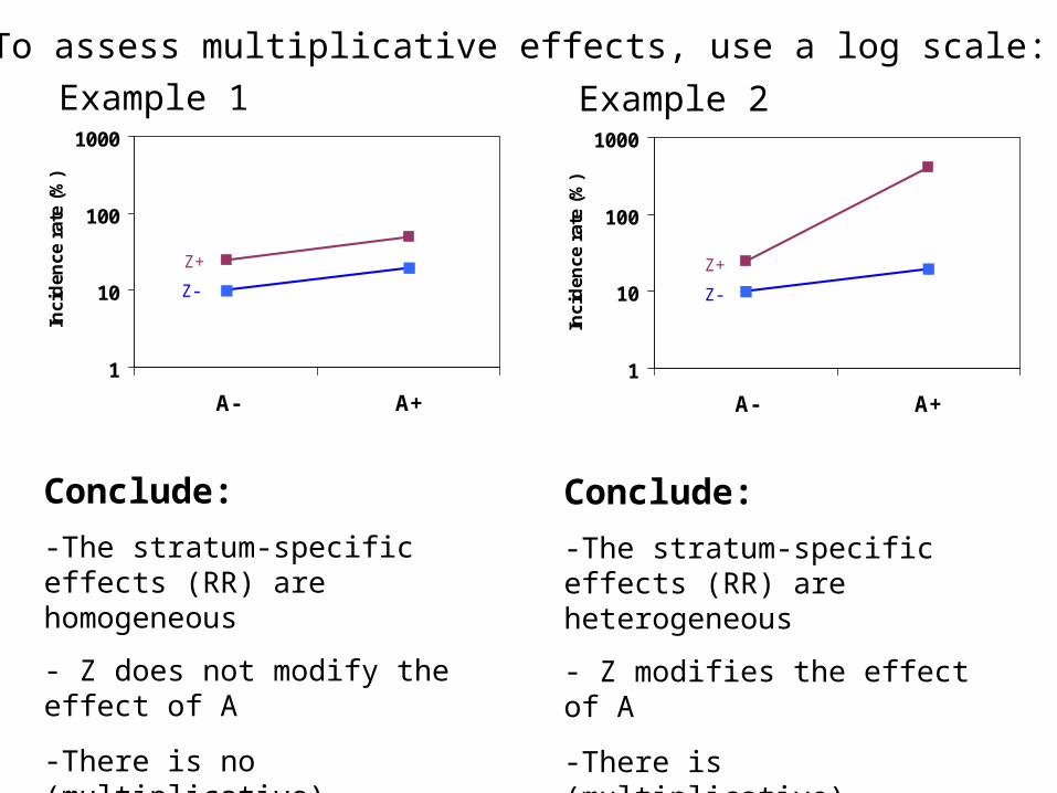
To assess multiplicative effects, use a log scale:
Conclude:
-The stratum-specific effects (RR) are homogeneous
- Z does not modify the effect of A
-There is no (multiplicative) interaction
1
10
100
1000
A- A+
Inci
den
ce r
ate
(%)
Z+
Z-
Conclude:
-The stratum-specific effects (RR) are heterogeneous
- Z modifies the effect of A
-There is (multiplicative) interaction
Example 1 Example 2
Two strategies to evaluate interaction based on different, but equivalent definitions:
• Effect modification (homogeneity/heterogeneity of effects)
• Comparison between joint expected and joint observed effects

Second strategy to assess interaction:(based on the calculation of “joint effects”)
A ZIndividual effects
Expected joint effect
+
Observed joint effect A+Z
No interaction
Observed joint effect A+Z
Synergism (Positive Interaction)
Observed joint effect A+Z
Antagonism (Negative Interaction)
+I
-I

The two definitions and strategies are completely equivalent. It is impossible to conclude that there is (or there is not) interaction using one strategy, and reach the opposite conclusion upon use of the other strategy!
Thus, when there is effect modification, the joint observed and the joint expected effects will be
different.

Factor Z
Factor A
Incidence (%)
Stratified ARA
ARvs(--)
No 10.0 No Yes 20.0
10.0
No 30.0 Yes Yes 40.0
10.0
Second strategy to assess interaction:comparison of joint expected and joint observed effects
Additive interaction
ReferenceReference
Reference

Factor Z
Factor A
Incidence (%)
Stratified ARA
ARvs(--)
No 10.0 No Yes 20.0
10.0
No 30.0 Yes Yes 40.0
10.0
10.020.030.0
Second strategy to assess interaction:comparison of joint expected and joint observed effects
Additive interaction
ReferenceReference
Reference
Independenteffects of:
A
Z A + Z

Factor Z Factor A Incidence (%)Stratified
ARA
ObservedARvs(--)
No 10.0 ReferenceNoYes 20.0 10.0No 30.0YesYes 40.0 10.0
10.020.030.0
Second strategy to assess interaction:comparison of joint expected and joint observed effects
Additive interaction
Conclude:Because the observed joint AR is the same as that expected by adding the individual AR’s, there is no additive interaction(that is, the same conclusion as when looking at the stratified AR’s)
Joint observedobserved ARA+Z+ = 30%Joint expectedexpected ARA+Z+ = ARA+Z- + ARA-Z+= 30%
Reference
Reference

Factor Z Factor A Incidence (%)Stratified
ARA
ObservedARvs(--)
No 5.0 ReferenceNoYes 10.0 5.0No 10.0YesYes 30.0 20.0
5.05.0
25.0 10.0
Expected
Second strategy to assess interaction:comparison of joint expected and joint observed effects
Additive interaction
Conclude:Because the observed joint AR is different from that expected by adding the individual AR’s, additive interaction is present(that is, the same conclusion as when looking at the stratified AR’s)
Joint observedobserved AR = 25%Joint expectedexpected AR = ARA+Z- + ARA-Z+= 10%
Reference
Reference
Factor Z
Factor A
Incidence (%)
Stratified RRA
RRvs(--)
No 10.0 Reference No Yes 20.0
2.0
No 25.0 Yes Yes 50.0
2.0
2.02.55.0
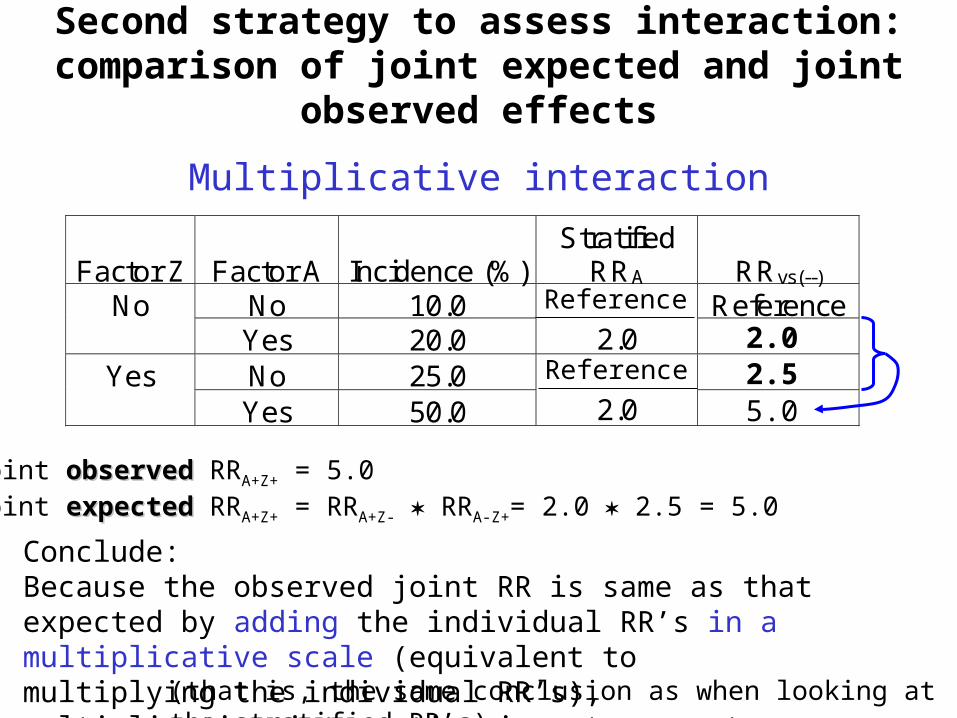
Second strategy to assess interaction:comparison of joint expected and joint observed effects
Multiplicative interaction
(that is, the same conclusion as when looking at the stratified RR’s)
Conclude:Because the observed joint RR is same as that expected by adding the individual RR’s in a multiplicative scale (equivalent to multiplying the individual RR’s), multiplicative interaction is not present
Joint observedobserved RRA+Z+ = 5.0Joint expectedexpected RRA+Z+ = RRA+Z- RRA-Z+= 2.0 2.5 = 5.0
Reference
Reference

Factor Z
Factor A
Incidence (%)
Stratified RRA
RRvs(--)
No 10.0 Reference No Yes 20.0
2.0
No 25.0 Yes Yes 125.0
5.0
5.0
2.02.5
12.5
Second strategy to assess interaction:comparison of joint expected and joint observed effects
Multiplicative interaction
Conclude:Since the observed joint RR is different from that expected by multiplying the individual RR’s, there is multiplicative interaction(that is, the same conclusion as when looking at the stratified RR’s)
Joint observedobserved RRA+Z+ = 12.5
Joint expectedexpected RRA+Z+ = RRA+Z- RRA-Z+= 2.0 2.5 = 5.0
Reference
Reference

How can we assess interaction in case-control studies?

First strategy to assess interaction:Effect Modification
Case-control study
Prospective Study
Z A Incidence rate (%) ARexp to A (%)
No No 5.0
5.0Yes 10.0
Yes No 10.0
20.0Yes 30.0
Additive interaction cannot be assessed in case-control studies by using the effect modification (homogeneity/heterogeneity) strategy, as no incidence rates are available to calculate attributable risks in the exposed
First strategy to assess interaction:Effect Modification
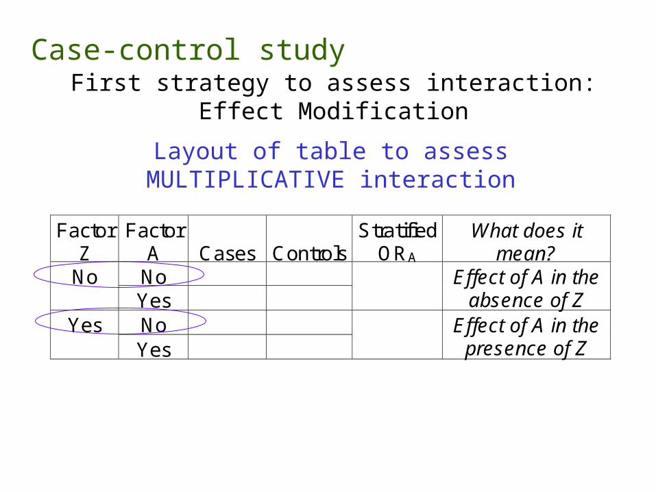
Layout of table to assessMULTIPLICATIVE interaction
Case-control study
Factor Z
Factor A
Cases
Controls
Stratified ORA
What does it mean?
No No Yes
Effect of A in the absence of Z
No Yes Yes
Effect of A in the presence of Z

Family history of clubfoot
Maternal smoking Cases Controls
Yes Yes 14 7
No 11 20
No Yes 118 859
No 203 2,143
Honein et al. Family history, maternal smoking, and clubfoot: an indication of gene-environment interaction. Am J Epidemiol 2000;152:658-65.
Odds Ratios for the association among isolated clubfoot, maternal smoking, and a family history of clubfoot, Atlanta, Georgia, 1968-80
Hypothesis: Family History is a potential effect modifier of the association between Maternal Smoking and clubfoot
Use the first strategy (homogeneity/heterogeneity) to evaluate the presence of multiplicative interaction

Family history of clubfoot
Maternal smoking Cases Controls
Stratified ORmaternal smk
Yes Yes 14 7 3.64
No 11 20
No Yes 118 859 1.45
No 203 2,143Honein et al. Family history, maternal smoking, and clubfoot: an indication of gene-environment interaction. Am J Epidemiol 2000;152:658-65.
Odds Ratios for the association among isolated clubfoot, maternal smoking, and a family history of clubfoot, Atlanta, Georgia, 1968-80
Conclude: Since the stratified ORs are different (heterogeneous), there is multiplicative interaction.
Now evaluate the same hypothesis (that there is an interaction between family history of clubfoot and maternal smoking) using the second strategy: comparison between joint observed and joint expected “effects”.
refe
renc
e
refe
renc
e

Second strategy to assess interaction:comparison of joint observed and expected effects
Layout of table to assess both ADDITIVEand MULTIPLICATIVE interaction
Case-control study
Factor Z
Factor A
Cases
Controls
ORvs--
What does it mean?
No 1.0 Reference No Yes Indep effect of A No Indep effect of Z Yes Yes Joint effect
Under ADDITIVE MODEL: Exp’d OR++ = OR+- + OR-+ - 1.0
OR-+
OR+-
OR++
Note common reference category

)()( IncIncIncIncIncIncARExpected
Inc
Inc
Inc
Inc
Inc
Inc
Inc
Inc
Inc
Inc
Inc
Inc
0.1 RRRRRR
If disease is “rare” (e.g., <5%):
0.1 OROROR
Derivation of formula for expected joint OR
observed
RR++ RR+- 1.0 RR-+ 1.01.0
expected

Derivation of formula: Expected OR++ = OR+- + OR-+ - 1.0
Intuitive graphical derivation:*
OR
1.0
2.02.5
3.5
Baseline+Excess due to A
Baseline+Excess due to Z
OR-- OR-+ OR+- Exp’dOR++
EXCZ
Baseline
BL
EXCA
BL
EXCZ
BL
EXCA
[EXCA+BL] + [EXCZ+BL] - BL
=
OR-+ + OR+- – 1.0
*For a more formal derivation, see Szklo & Nieto, pp. 229-230 (not required).
BL

OR
1.0
2.02.5
3.5 3.5
OR-- OR-+ OR+- Exp’dOR++
Observed OR++
Conclude:If the observed joint OR is the same as the expected under the additive model, there is no additive interaction

OR
1.0
2.02.5
3.5
6.0
OR-- OR-+ OR+- Exp’dOR++
Observed OR++
Conclude:If the observed joint OR is different than the expected under the additive model, there is additive interaction
Excess due tointeraction (“interaction term”)
Excess due to thejoint effects of A and Z
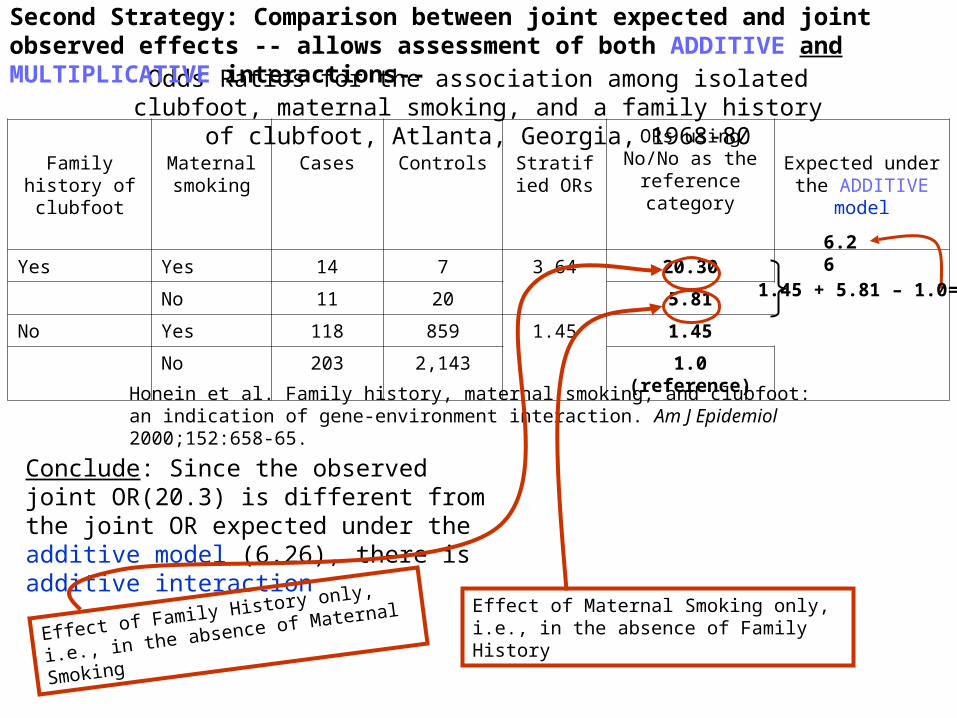
Family history of clubfoot
Maternal smoking
Cases Controls Stratified ORs
ORs using No/No as the reference
categoryExpected under the ADDITIVE model
Yes Yes 14 7 3.64 20.30
No 11 20 5.81
No Yes 118 859 1.45 1.45
No 203 2,143 1.0 (reference)
Honein et al. Family history, maternal smoking, and clubfoot: an indication of gene-environment interaction. Am J Epidemiol 2000;152:658-65.
Odds Ratios for the association among isolated clubfoot, maternal smoking, and a family history of clubfoot, Atlanta, Georgia, 1968-80
Conclude: Since the observed joint OR(20.3) is different from the joint OR expected under the additive model (6.26), there is additive interaction
Effect of Maternal Smoking only, i.e., in the absence of Family HistoryEffect of Family History only, i.e., in the
absence of Maternal Smoking
6.26
1.45 + 5.81 – 1.0=
Second Strategy: Comparison between joint expected and joint observed effects -- allows assessment of both ADDITIVE and MULTIPLICATIVE interactions--

Second strategy to assess interaction:comparison of joint observed and expected effects
Layout of table to assess both ADDITIVEand MULTIPLICATIVE interaction
Case-control study
Factor Z
Factor A
Cases
Controls
ORvs--
What does it mean?
No 1.0 Reference No Yes Indep effect of A No Indep effect of Z Yes Yes Joint effect
Under ADDITIVE MODEL: Exp’d OR++ = OR+- + OR-+ - 1.0
OR-+
OR+-
OR++
Under MULTIPLICATIVE MODEL: Exp’d OR++ = OR+- OR-+

Family history of clubfoot
Maternal smoking
Cases Controls Stratified ORs
ORs using No/No as the reference
categoryExpected under the
MULT. model
Yes Yes 14 7 3.64 20.30
No 11 20 5.81
No Yes 118 859 1.45 1.45
No 203 2,143 1.0 (reference)
Honein et al. Family history, maternal smoking, and clubfoot: an indication of gene-environment interaction. Am J Epidemiol 2000;152:658-65.
Odds Ratios for the association among isolated clubfoot, maternal smoking, and a family history of clubfoot, Atlanta, Georgia, 1968-80
Conclude: Since the observed joint OR(20.3) is different from the joint OR expected under the multiplicative model(8.42), there is multiplicative interaction
Effect of Maternal Smoking only, i.e., in the absence of Family HistoryEffect of Family History only, i.e., in the
absence of Maternal Smoking
8.42
1.45 5.81 =

Back to the terms...• Synergism or Synergy: The observed joint “effect” is
greater than that expected from the individual “effects”.
Which is equivalent to saying that the “effect” of A in the presence of Z is stronger than the “effect” of A when Z is absent.
• Antagonism: The observed joint “effect” is smaller than that expected from the individual “effects”.
Which is equivalent to saying that the “effect” of A in the presence of Z is weaker than the “effect” of A when Z is absent
Note: the expressions “synergism/antagonism” and “effect modification” should ideally be reserved for situations in which one is sure of a causal connection. In the absence of evidence supporting causality, it is preferable to use terms such as “heterogeneity” or “positive/negative interaction”.

Terminology
• Positive interaction = Synergism = “More than additive effect” (for the additive model) or “More than multiplicative effect” (for the multiplicative model)
• Negative interaction = Antagonism = “Less than additive/multiplicative effect”
Some investigators reserve the term “synergy” to define a biologically plausible interaction

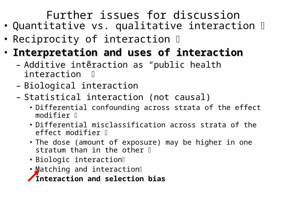
Further issues for discussion
• Quantitative vs. qualitative interactionQuantitative vs. qualitative interaction

Family history of clubfoot
Maternal smoking Cases Controls
Stratified ORmaternal smk
Yes Yes 14 7 3.64
No 11 20
No Yes 118 859 1.45
No 203 2,143Honein et al. Family history, maternal smoking, and clubfoot: an indication of gene-environment interaction. Am J Epidemiol 2000;152:658-65.
Odds Ratios for the association among isolated clubfoot, maternal smoking, and a family history of clubfoot, Atlanta, Georgia, 1968-80
Quantitative interaction: both ORs are in the same direction(>1.0), but they are heterogeneous

Am J Epidemiol 1995;142:1322-9
Smoking Caffeine No. pregnanciesDelayed
conception>12 months
StratifiedORA 95% CI
No 575 47No301 mg/d 90 17 2.62 1.36-4.98
No 76 15Yes301 mg/d 83 11 0.62 0.27-1.45
Reproductive Health Study, retrospective study of 1,430 non-contraceptive parous women, Fishkill, NY, Burlington, VT, 1989-90.
Odds ratios are not only different; they have different directions (>1, and <1). Smoking modifies the effect of caffeine on delayed conception in a qualitative manner, i.e., there is qualitative interaction.

When there is qualitative interaction in one scale (additive or multiplicative), it
must also be present in the other
A- A+
Ris
k of
ou
tcom
e
Z-
Z+ RRA
>1
<1
ARA
Positive (>0)
Negative (<0)
Z+Z-
Qualitative Interaction:
Effect Modifier Risk Factor Incidence/1000 ARA RRA
Z+ A+ 10.0 +5/1000 2.0
A- 5.0 Reference 1.0
Z- A+ 3.0 -3/1000 0.5
A- 6.0 Reference 1.0
Interaction in both scales

When there is qualitative interaction in one scale (additive or multiplicative), it must
also be present in the other
A- A+
Ris
k of
ou
tcom
e
Z-
Z+ ARA
Positive (>0)
Negative (<0)
RRA
>1
<1
Z+Z-
Qualitative Interaction:
Effect Modifier Risk Factor Incidence/1000 ARA RRA
Z+ A+ 10.0 +5/1000 2.0
A- 5.0 Reference 1.0
Z- A+ 3.0 -3/1000 0.5
A- 6.0 Reference 1.0

When there is qualitative interaction in one scale (additive or multiplicative), it must
also be present in the other
A- A+
Ris
k of
ou
tcom
e
Z-
Z+ ARA Positive (>0)
Negative (<0)
RRA
>1
<1
Z+Z-
“cross-over”
A- A+
Ris
k of
ou
tcom
e
Z-
Z+ ARA
Positive (>0)
Null (=0)
RRA
>1
=1
Z+Z-
Another type of qualitative interaction: “effect”of A is flat in one stratum of the effect modifier; in the other stratum, an association is observed

Circulation 2000;101:2034-9
Age-adjusted HR of CHD:
Normotensive persons
Anger score
Low Moderate High
1.00 1.36 2.97
Hypertensive persons
Anger score
Low Moderate High
1.00 0.88 1.05
Example of qualitative interaction
(CHD)(CHD)
CHD event-free survival probabilities among normotensivenormotensive individuals by trait anger scores
Days of follow-up
CHD event-free survival probabilities among hypertensive hypertensive individuals by trait anger scores
Days of follow-up
LowModerate
High
Anger score:Low (10-14)Moderate (15-21High (22-40)
CH
D-f
ree
cu
mu
lati
ve
pro
ba
bil
itie
s

Further issues for discussion
• Quantitative vs. qualitative interaction• Reciprocity of interactionReciprocity of interaction
If Z modifies the effect of A on disease Y, then Z will necessarily modify the effect of Z on disease Y

Reciprocity of interactionThe decision as to which is the “principal” variable and which is the
effect modifier is arbitrary, because if A modifies the effect of Z, then Z modifies the effect of A.
Factor Z
Factor A
Incidence (%)
Stratified RRA
RRvs(--)
No 10.0 Reference No Yes 20.0
2.0 2.0
No 25.0 2.5 Yes Yes 125.0
5.0 12.5
Z modifies the effect of A
Factor A Factor Z Incidence (%)Stratified
RRZ RRvs(--)
No 10.0 ReferenceNoYes 25.0 2.5 2.5No 20.0 2.0YesYes 125.0 6.25 12.5
A modifies the effect of Z

Matched case-control study (matching by gender) of the relationship of risk factor X (e.g., alcohol drinking ) and
disease Y (e.g., esophageal cancer)
Pair No. Case Control OR by gender
1 (male) + -
2 (male) + -
3 (male) - +
4 (male) + -
5 (male) + +
6 (female) - -
7 (female) + -
8 (female) - +
9 (female) + +
10 (female) - -
Total (Pooled) Odds Ratio
INTERACTION IS NOT CONFOUNDING

Matched case-control study (matching by gender) of the relationship of risk factor X (e.g., alcohol drinking ) and
disease Y (e.g., esophageal cancer)
Pair No. Case Control OR by gender
1 (male) + -
2 (male) + -
3 (male) - +
4 (male) + -
5 (male) + +
6 (female) - -
7 (female) + -
8 (female) - +
9 (female) + +
10 (female) - -
Total (Pooled) Odds Ratio 4/2= 2.0
INTERACTION IS NOT CONFOUNDING

Matched case-control study (matching by gender) of the relationship of risk factor X (e.g., alcohol drinking ) and
disease Y (e.g., esophageal cancer)
Pair No. Case Control OR by sex
1 (male) + -
3/1 = 3.02 (male) + -
3 (male) - +
4 (male) + -
5 (male) + +
6 (female) - -
1/1= 1.07 (female) + -
8 (female) - +
9 (female) + +
10 (female) - -
Total (Pooled) Odds Ratio 4/2= 2.0
INTERACTION IS NOT CONFOUNDING

Further issues for discussion
• Quantitative vs. qualitative interaction
• Reciprocity of interaction
• Interpretation and uses of interactionInterpretation and uses of interaction– Additive interaction as “public health Additive interaction as “public health
interaction”interaction” (term coined by Rothman)

Current Smoking Status
Low Vitamin C intake (mg/day)
Odds Ratio
No No 1.0
Yes No 6.8
No Yes 1.8
Yes Yes 10.6
Joint effects of current cigarette smoking and low consumption of vitamin C (≤ 100 mg/day) with regard to adenocarcinoma of the salivary gland, San Francisco-Monterey
Bay area, California, 1989-1993
(Horn-Ross et al. Diet and risk of salivary gland cancer. Am J Epidemiol 1997;146:171-6)
Additive Model:Expected joint Odds Ratio = 6.8 + 1.8 – 1.0= 7.6
Positive additive interaction=
“Public Health interaction”
Multiplicative Model:Expected joint Odds Ratio = 6.8 1.8 = 12.4
ConcludeConclude: For Public Health purposes, ignore negative multiplicative interaction, and focus on : For Public Health purposes, ignore negative multiplicative interaction, and focus on smokers for prevention of low vitamin C intakesmokers for prevention of low vitamin C intake
Negative multiplicative interaction

Additive interaction as “Public Health interaction”
Incidence per 100
Family history (EM)
Smoking (RF)
Stratified ARSmk%
Stratified RRSmk
5.0 No No
10.0 Yes
5.0
2.0
20.0 Yes No
30.0 Yes
10.0
1.5
Incidence of disease “Y” by smoking and family history of “Y”
Thus, if there are enough subjects who are positive for both variables and if resources are limited, smokers with a positive family history should be regarded as the main “target” for prevention examine the prevalence of (Fam HIst+ and Smk+ ) and estimate the attributable risk in the population
Positive additive interaction (synergism), but negative
multiplicative interaction (antagonism)
EM- effect modifierRF- risk factor of interest

Further issues for discussion
• Quantitative vs. qualitative interaction • Reciprocity of interaction • Interpretation and uses of interactionInterpretation and uses of interaction
– Additive interaction as “public health interaction” – Biological interaction

Am J Epidemiol 1995;142:1322-9
Smoking Caffeine No. pregnanciesDelayed
conception>12 months
StratifiedORA 95% CI
No 575 47No301 mg/d 90 17 2.62 1.36-4.98
No 76 15Yes301 mg/d 83 11 0.62 0.27-1.45
Reproductive Health Study, retrospective study of 1,430 non-contraceptive parous women, Fishkill, NY, Burlington, VT, 1989-90.
“…An interaction between caffeine and smoking is also biologically plausible. Several studies have shown that cigarette smoking significantly increases the rate of caffeine metabolism […]. The accelerated caffeine clearance in smokers may explain why we failed to observe an effect of high caffeine consumption on fecundability among women who smoked cigarettes.”
This interaction can be properly named, “synergy”, as it has a strong biological plausibility

Further issues for discussion
• Quantitative vs. qualitative interaction • Reciprocity of interaction • Interpretation and uses of interactionInterpretation and uses of interaction
– Additive interaction as “public health interaction” – Biological interaction– Statistical interaction (not causal)
• Differential confoundingDifferential confounding
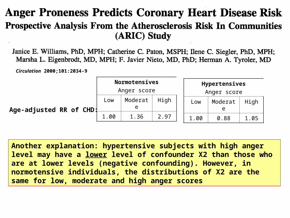
Circulation 2000;101:2034-9
Age-adjusted RR of CHD:
Normotensives
Anger score
Low Moderate High
1.00 1.36 2.97
Hypertensives
Anger score
Low Moderate High
1.00 0.88 1.05
Another explanation: hypertensive subjects with high anger level may have a lower level of confounder X2 than those who are at lower levels (negative confounding). However, in normotensive individuals, the distributions of X2 are the same for low, moderate and high anger scores

Prevalence of G
Incidence Relative Risk
MenMen
Exposed 0.8 [(0.8 0.04 ) + (0.2 0.02)] 100= 3.6%
1.6
Unexposed 0.1 [(0.10 0.04) + (0.90 0.02)] 100 = 2.2%
1.0
WomenWomen
Exposed 0.20 [(0.20 0.04) + (0.80 0.02)] 100= 2.4%
1.0
Unexposed 0.20 [(0.20 0.04) + (0.80 0.02)] 100= 2.4%
1.0
• No association between the exposure (e.g., chewing gum) and the disease (e.g., liver cancer)• Unaccounted-for confounder (e.g., a genetic polymorphism G)• Incidence of the disease by G:
G+ = 0.04 G- = 0.02
Example of confounding resulting in apparent interaction

Further issues for discussion
• Quantitative vs. qualitative interaction • Reciprocity of interaction • Interpretation and uses of interactionInterpretation and uses of interaction
– Additive interaction as “public health interaction” – Biological interaction– Statistical interaction (not causal)
• Differential confounding across strata of the effect modifier
• Misclassification resulting from different sensitivity and specificity values of the variable under study across strata of the effect modifier

Smoking Status BMI status Cases Controls Odds Ratio
Smokers Overweight 200 100 2.25
Not overweight 800 900
Non-smokers Overweight 200 100 2.25
Not overweight 800 900
Example of effect of misclassification of overweight by smoking category, on the Odds Ratios

SmokersSmokers: Cases Controls
Sensitivity 0.80 0.80
Specificity 0.85 0.85
Non-smokersNon-smokers: Cases Controls
Sensitivity 0.95 0.95
Specificity 0.98 0.98
Smokers
Over- weight
Cases Controls ORMISCL
Yes 280 215 1.4
No 720 785
Non-Smokers
Over- weight
Cases Controls ORMISCL
Yes 206 113 2.0
No 794 887
Smoking Status BMI status Cases Controls Odds RatioTRUE
Smokers Overweight 200 100 2.25
Not overweight 800 900
Non-smokers Overweight 200 100 2.25
Not overweight 800 900
Non-differential misclassification within each stratum
Values of indices of validity different between smokers and non-smokers

Further issues for discussion
• Quantitative vs. qualitative interaction • Reciprocity of interaction • Interpretation and uses of interactionInterpretation and uses of interaction
– Additive interaction as “public health interaction” – Biological interaction– Statistical interaction (not causal)
• Differential confounding across strata of the effect modifier
• Differential misclassification across strata of the effect modifier
• The dose (amount of exposure) may be higher in one stratum than in the other

Usually drank liquor with nonalcoholic mixers (n= 163)
Usually drank liquor straight (undiluted) (n= 206)
Drinks/week Odds Ratio (95% CI) Odds Ratio (95% CI)
>0 - <8 1.0 (reference) 3.2 (1.4, 7.2)
8 - <22 1.0 (0.3, 3.0) 4.2 (1.7, 10.5)
22 - <43 3.6 (1.2, 10.8) 7.9 (3.0, 21.3)
43 - <64 6.2 (1.2, 31.1) 8.3 (2.3, 29.4)
64 - <137 1.1 (0.2, 5.4) 23.5 (6.8, 81.5)
Oral cancer odds ratios* related to consumption of diluted and undiluted forms of liquor by liquor drinkers, Puerto Rico, 1992-1995
*Adjusted for age, tobacco use, consumption of raw fruits and vegetables, and educational level

Gender Smoking Relative Risk
Man Yes 3.0
No 1.0
Woman Yes 1.5
No 1.0
Exposure duration and interaction
Are you surprised??
When studying effects of smoking in men and women, the category “smoker” is related to more cigarettes/day in men than in women. Thus, the observed odds ratios may be heterogeneous because of different levels of smoking exposure between men and women, and not because men are more susceptible to smoking-induced disease.

Further issues for discussion• Quantitative vs. qualitative interaction • Reciprocity of interaction • Interpretation and uses of interactionInterpretation and uses of interaction
– Additive interaction as “public health interaction” – Biological interaction– Statistical interaction (not causal)
• Differential confounding across strata of the effect modifier • Differential misclassification across strata of the effect modifier • The dose (amount of exposure) may be higher in one stratum than in
the other• Biologic interaction:
– Consistent with pathophysiologic mechanisms (biologic plausibility)
– Confirmed by animal studies– What is best model from the biologic viewpoint?
No one knows for sure… Think about the specific condition under study – Examples: trauma, cancer
Problem: Epidemiology usually assesses proximal cause X1 X2 X3 Y

10
20
30
40
50
60
70
Normal artery
Fatty streaks
Fibrous plaque
Myocardial infarct
Cerebral infarct
Gangrene of extremities
Abdominal aortic
aneurism
clinical horizon
Age
in y
ears
Schematic view of the development of atherosclerosis. Based on McGill et al, in Atherosclerosis and Its Origins, M Sandler & G Bourne, eds, p. 42, © 1963, Academic Press
Endothelial dysfunction (no anatomical expression)
CalcificationComplicated lesion- hemorrhage, ulceration, thrombosis
Intimal-medial thickening

Y1 Y2 Y3 --> ….YZ-1 YZX1
X2 X3 X3 XZ
Usual realm of epidemiologic studiesProximal relationship:
Natural History of of Disease

Normal Fatty streaks
Intima-media thicknening
Endothelial dysfunction
Fibrous plaque:•Stable
•Unstable
Clinical events (CHD, LEAD,
etc)
Smoking
Sharrett AR, et al. Atherosclerosis 2004;172:143-149
ARIC
hemorrhage, thrombosis
LDL

Y1 Y2 Y3 --> ….YZ-1 YZX1
X2 X3 X3 XZ
additive
additive
EM or RF 1
EM or RF 2
multiplic
ative
multiplic
ative
Usual realm of epidemiologic studiesProximal relationship:
Natural History of of Disease

AtherosclerosisHigh blood pressure: endothelial injury/trauma: additive model?
Multiplication (and migration) of medial smooth muscle cells multiplicative?
mediaintima
Blood flow
First event
Second event

Further issues for discussion• Quantitative vs. qualitative interaction • Reciprocity of interaction • Interpretation and uses of interactionInterpretation and uses of interaction
– Additive interaction as “public health interaction” – Biological interaction– Statistical interaction (not causal)
• Differential confounding across strata of the effect modifier • Differential misclassification across strata of the effect modifier • The dose (amount of exposure) may be higher in one stratum than in
the other • Biologic interaction• Matching and interaction
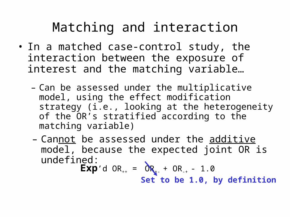
Matching and interaction
• In a matched case-control study, the interaction between the exposure of interest and the matching variable…
– Can be assessed under the multiplicative model, using the effect modification strategy (i.e., looking at the heterogeneity of the OR’s stratified according to the matching variable)
Exp’d OR++ = OR+- + OR-+ - 1.0Set to be 1.0, by definition
– Cannot be assessed under the additive model, because the expected joint OR is undefined:

Matched case-control study (matching by gender) of the relationship of risk factor X (e.g., alcohol drinking ) and
disease Y (e.g., esophageal cancer)
Pair No. Case Control OR by sex
1 (male) + -
3/1 = 3.02 (male) + -
3 (male) - +
4 (male) + -
5 (male) + +
6 (female) - -
1/1= 1.07 (female) + -
8 (female) - +
9 (female) + +
10 (female) - -
Total (Pooled) Odds Ratio 4/2= 2.0
INTERACTION IS NOT CONFOUNDING
Further issues for discussion• Quantitative vs. qualitative interaction • Reciprocity of interaction • Interpretation and uses of interactionInterpretation and uses of interaction
– Additive interaction as “public health interaction” – Biological interaction– Statistical interaction (not causal)
• Differential confounding across strata of the effect modifier • Differential misclassification across strata of the effect modifier • The dose (amount of exposure) may be higher in one stratum than in
the other • Biologic interaction• Matching and interaction• Interaction and selection bias
Z+RRX= 3.0
Z-RRX= 3.0
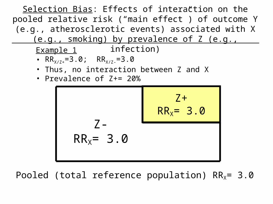
Example 1 • RRX/Z+=3.0; RRX/Z-=3.0• Thus, no interaction between Z and X• Prevalence of Z+= 20%
Selection Bias: Effects of interaction on the pooled relative risk (“main effect”) of outcome Y (e.g., atherosclerotic events) associated with X (e.g., smoking) by prevalence of Z (e.g.,
infection)
Pooled (total reference population) RRX= 3.0

Z-RRX= 3.0
Z+ RRX= 3.0
Not included or censored
Included and not censored
Relative Risk in those not lost to follow-up= 3.0 representative of RR of the total reference population
Example 1 • RRX/Z+=3.0; RRX/Z-=3.0• Thus, no interaction between Z and X• Prevalence of Z+= 20%

Z+RRX= 3.0
Z-RRX= 1.0
Pooled (total population) RRX= 1.4
Example 2• RRX/Z+=3.0; RRX/Z-=1.0• Thus, interaction between Z and X• Prevalence of Z+= 20%

Included and not censored
Not included or censored
Z+RRX= 3.0
Z-RRX= 1.0
Example 2• RRX/Z+=3.0; RRX/Z-=1.0• Thus, interaction between Z and X• Prevalence of Z+= 20%
Relative Risk in those not lost to follow-up= 1.0 NOT representative of RR of the total reference population

Z+ = 50%
Z+
= 1
0%
Pooled RRX = 1.2
Z+ =
50%
Z+ = 100%
Pooled RRX = 3.0 Pooled RRX = 1.0
Z+ =0%
Effects of interaction on the pooled relative risk (“main effect”) of outcome Y associated with X, by prevalence of the effect modifier Z
(RRX/Z+=3.0; RRX/Z-=1.0)
Z+ = 50%
Pooled RRX = 2.0
Z+ = 50%

Further issues for discussion• Quantitative vs. qualitative interaction • Reciprocity of interaction • Interpretation and uses of interactionInterpretation and uses of interaction
– Additive interaction as “public health interaction” – Biological interaction– Statistical interaction (not causal)
• Differential confounding across strata of the effect modifier • Differential misclassification across strata of the effect modifier • The dose (amount of exposure) may be higher in one stratum than in
the other • Biologic interaction• Matching and interaction• Interaction and selection bias• Interaction and adjustmentInteraction and adjustment

40
WW
BW
Age (years)
Bre
ast
Can
cer
Inci
den
ce R
ates
Interaction between age and ethnic background
“cross-over”

Adjustment and Interaction
Age A (e.g., exposed)
B (e.g., unexposed)
N Rate (%)
N Rate (%)
ARexp
RR
<50 100 20 200 10 10% 2.00
50+ 200 50 100 40 10% 1.25
• Note that ARs are the same, butRR’s are different
Multiplicative interaction

Standard PopulationsAge
Population B Arbitrary Minimumvariance
<50 200 1800 66.7
50+ 100 200 66.7
A B A B A BAdj.Rate 30% 20% 23% 13% 35% 25%
ARexp 10% 10% 10%
RR 1.5 1.8 1.4
• For younger standard populations (e.g., arbitrary), the “adjusted” RR will approximate the rate seen in those who are <50 years old
• For older standard populations (e.g., minimum variance), the adjusted RR will approximate the AR seen in those who are 50+ years old
• Because there is no interaction in the additive (AR) scale, the composition of the standard population is irrelevant, and the adjusted ARs are always the same regardless of the standard
Age A B
N Rate (%)
N Rate (%)
ARexp
RR
<50 100 20 200 10 10% 2.00
50+ 200 50 100 40 10% 1.25
When Relative Risks are heterogeneous, the adjusted RR varies according to the composition of the effect modifier in the standard
population

Adjustment and Interaction
Age A B
N Rate (%)
N Rate (%)
ARexp
RR
<50 100 6 200 3 3% 2.0
50+ 200 30 100 16 15% 2.0
• Note that RRs are the same, butARexp’s are different
Additive interaction

Standard PopulationsAge
Population B Arbitrary Minimumvariance
<50 200 1800 66.7
50+ 100 200 66.7
A B A B A BAdj.Rate 14% 7% 8.4% 4.2% 18% 9%
ARexp 7% 4.2% 9.0%
RR 2.0 2.0 2.0
Age A B
N Rate(%)
N Rate(%)
ARexp RR
<50 100 6 200 3 3% 2.0
50+ 200 30 100 16 15% 2.0
• For younger standard populations (e.g., arbitrary), the “adjusted” AR will approximate the rate seen in those who are <50 years old
• For older standard populations (e.g., minimum variance), the adjusted AR will approximate the AR seen in those who are 50+ years old
• Because there is no interaction in the multiplicative scale, the composition of the standard population is irrelevant, and the adjusted RRs are always the same, regardless of the standard
When Attributable Risks in the exposed are heterogeneous, the adjusted AR varies according to the composition of the effect
modifier in the standard population

Conclusion
• If heterogeneity is present… is there interaction?– What is the magnitude of the difference? (p-value?)
– Is it qualitative or just quantitative?– Is it biologically plausible?
• If we conclude that there is interaction, what should we do?
– Report the stratified measures of association … The interaction may be the most important finding of the study!