interactions between auditory and visual motion …

INTERACTIONS BETWEEN AUDITORY AND VISUAL MOTION MECHANISMS AND THE ROLE OF ATTENTION:

PSYCHOPHYSICS AND QUANTITATIVE MODELS

By

ANSHUL JAIN

A Dissertation submitted to the

Graduate School-New Brunswick

Rutgers, The State University of New Jersey

and

The Graduate School of Biomedical Sciences

University of Medicine and Dentistry of New Jersey

in partial fulfillment of the requirements

for the degree of

Doctor of Philosophy

Graduate Program in Biomedical Engineering

written under the direction of

Dr. Thomas V. Papathomas

and approved by

________________________

________________________

________________________

________________________

________________________

New Brunswick, New Jersey October 2008

ii

ABSTRACT OF THE DISSERTATION

Interactions between Auditory and Visual Motion Mechanisms and

the Role of Attention: Psychophysics and Quantitative Models

By ANSHUL JAIN

Dissertation Director:

Thomas V. Papathomas

The human brain continuously receives sensory input from the dynamic physical world via various

sensory modalities. In many cases, a single physical event generates simultaneous input to more

than one modality. For example, a ball hitting the ground generates both visual and auditory

input. The human brain has developed mechanisms to take advantage of the correlations

between inputs to different modalities to form a uniform and stable percept. Recently, there has

been a lot of research interest, psychophysical, neurophysiological and computational, to explore

the mechanisms involved in crossmodal interactions in general and auditory-visual interactions in

particular.

The current thesis makes three significant contributions to the field of auditory-visual interactions.

First, I designed a comprehensive study to psychophysically examine the interactions between

auditory and visual motion mechanisms for three different motion configurations: horizontal,

vertical and motion-in-depth. I showed that simultaneous presentation of a strong motion signal in

one modality influences perception of a weak motion signal in the other modality both when the

iii

weak motion in presented in the visual, as well as in the auditory modality. I further observed that

crossmodal aftereffects were induced only when subjects adapted to spatial motion in the visual

modality and not in the auditory modality. However, adaptation to auditory spectral motion did

induce vertical visual motion aftereffects. To my knowledge, this is the first report of auditory-

induced visual aftereffects. Second, I conducted psychophysical experiments to study the effects

of spectral attention on the visual and the auditory motion mechanisms and showed that there are

similar attentional effects on motion mechanisms within the two modalities. Third, I developed a

neurophysiologically relevant computational model to provide a possible explanation for

crossmodal interactions between the auditory and the visual motion mechanisms. In addition, I

developed a model that can explain the observed experimental findings on the role of spectral

attention in modulating motion aftereffects. The results obtained from both the model simulations

agree very closely with the human behavioral data obtained from the experiments.

iv

ACKNOWLEDGEMENT AND DEDICATION

First and foremost, I thank my advisor, Dr. Thomas V. Papathomas. This work would not have

been possible without his scientific guidance. He was always available for discussions and

explained things very clearly and constantly encouraged me to work on my own ideas. His

enthusiasm always motivated me to stay focused and he has always been a source of inspiration.

I express my sincerest gratitude to Thomas.

I also thank Dr. Sharon Sally for her involvement with the experiments on crossmodal

interactions. I deeply appreciate the valuable feedback provided by the members of the

committee, Dr. Madabhushi, Dr. Semmlow, Dr. Shinbrot and Dr. Singh. It certainly helped

improve the quality of this work.

I am grateful to fellow members of the lab, Ms. Xiaohua Zhuang, Dr. Xiaotao Su, Ms. Aleksandra

Sherman and Dr. Sunnia Chai for making my stay here truly enjoyable. I sincerely thank all the

members of the administrative staff at RuCCS, particularly Ms. Jo’Ann Meli and Ms. Sue

Cosentino for all their help with administrative matters and for getting the coffee machine installed

in the copy room. It saved me many long walks to the student center.

I am indebted to all my friends at Rutgers, fellow graduate students in the Biomedical Engineering

department and last but not the least my soccer group for giving me numerous memories that I

will cherish for the rest of my life. I always looked forward to the pick-up games and intramural

matches.

Finally, I thank my parents Shanta and Janak for their endless love and care. I thank my wife,

Nithya, for being by my side through the entire journey and putting up with everything that the

wife of a graduate student has to put up with. I would not have come this far without her love,

v

support and constant encouragement. I thank my sister Sonal, my brother Pankaj and his family

for their support and the sound advice they gave me at critical junctures throughout my life.

I dedicate this dissertation to my family, especially to my wife and my parents.

vi

TABLE OF CONTENTS

Abstract ……………………………………………………………………………….. ii

Acknowledgements and Dedications ……………………………………………… iv

List of Figures …………………………………...…………………………………… viii

List of Tables ………………………………………………………………………… xiii

Chapter 1 – Introduction …………………………………………………………… 1

1.1. Interactions between auditory and visual motion mechanisms ……. 2

1.2. The role of selective attention to spectral components in visual and

auditory motion perception …………………………………………….. 5

1.3. Computational model for interactions between auditory and visual

motion mechanisms ……………………………………………………. 7

1.4. Applications in Biomedical Engineering and other engineering fields 9

Chapter 2 – Interactions between Auditory and Visual Motion Mechanisms 11

2.1. General Methods ……………………………………………………….. 13

2.2. Experiment 1 – Transient Effects: Simultaneous Presentation ……. 17

2.3. Experiment 2 – Cross-modal visual/auditory motion aftereffects …. 31

2.4. General Discussion …………………………………………………….. 41

2.5. Conclusions …………………………………………………………….. 47

vii

Chapter 3 - The Role of Selective Attention to Spectral Features in Visual

and Auditory Motion Perception …………………………………………………. 49

3.1. Experiment 1 – Visual Spectral Attention …………………………… 51

3.2. Experiment 2 – Auditory Spectral Attention ………………………… 64

3.3. General Discussion and Conclusions ……………………………….. 77

Chapter 4 – Computational Model for Interactions between Auditory and

Visual Motion Mechanisms ………………………………………………………… 80

4.1. Unimodal Auditory and Visual Motion Processing ………………….. 81

4.2. Biased-Competition Model …………………………………………….. 85

4.3. Computational model for crossmodal interactions between auditory

and visual motion mechanisms ………………………………………. 87

4.4. Computation Model for Horizontal Motion Configuration …………… 88

4.5. Computation Model for Vertical Motion Configuration ……………… 105

4.6. Computation Model for Motion-in-depth Configuration ……………... 113

4.7. Computational model for attentional modulation of motion aftereffects

within the auditory and the visual modality …………………………….. 121

4.8. Conclusions ……………………………………………………………….. 129

Chapter 5 - Conclusions and Scope for Future Work ………………………… 131

5.1. Interactions between the auditory and visual motion mechanisms .. 132

5.2. The role of selective attention to spectral features in visual and

auditory motion perception …………………………………………… 134

5.3. Computational models …………………………………………………. 135

References …………………………………………………………………………… 139

Curriculum Vita ……………………………………………………………………… 145

viii

LIST OF FIGURES

Figure 2.1 The two horizontal motion stimuli. (a) Low-contrast superimposed

gratings, no motion signal in fovea. (b) High-contrast single

grating ……………………...………………………………………….. 14

Figure 2.2 Visual and auditory pairings used in the experiments. The left

panel shows the auditory stimuli while the right panel shows the

visual stimuli. The top, middle and bottom panel show the motion

along x-, y- and z-axes respectively ………………………………… 16

Figure 2.3 Psychometric curves for the six subjects that participated in the

horizontal motion configuration in Experiment 1b. Primary

Modality: Audition …………………………………………………… 21



Modality: Vision ……………………………………………………… 22

Figure 2.5 Psychometric curves averaged across subjects for horizontal

motion configuration in Experiment 1b. Top Panel: Primary

Modality – Audition. Bottom Panel: Primary Modality – Vision 23

Figure 2.6 Average PSEs for various conditions in Experiment 1 …………… 25

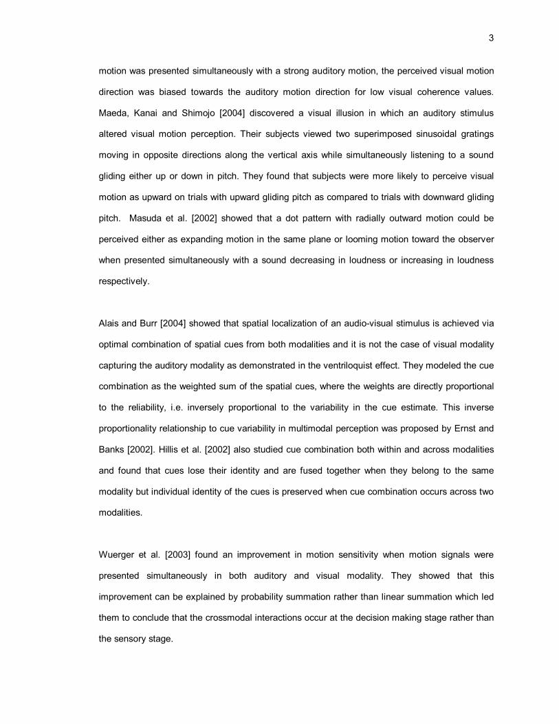
Figure 2.7 Average PSEs for vertical motion configuration when vertical

motion instead of spectral motion was used in Experiment 1a … 26

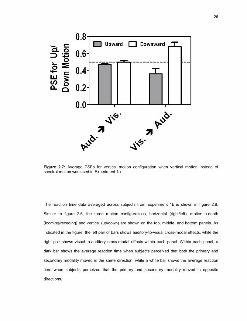
Figure 2.8 Average reaction times from Experiment 1b ……………………… 27

Figure 2.9 First and subsequent two trials of a typical block of trials in

Experiment 2 …………………………………………………………… 31



Modality: Audition …………………………………………………… 35

ix



Modality: Vision ………………………………………………………. 36

Figure 2.12 Psychometric curves averaged across subjects for horizontal

motion configuration in Experiment 2b. Top Panel: Primary

Modality – Audition Bottom Panel: Primary Modality – Vision … 37

Figure 2.13 Average PSEs for various conditions in Experiment 2 …………… 39

Figure 3.1 A single frame of the adapting stimulus. The 0.5 cycles/degrees

grating has been assigned color green, while the 2 cycles/

degrees grating has been assigned the red color ………………… 54

Figure 3.2 A single frame of the adapting stimulus. The 0.5 cycles/degrees

grating has been assigned color red, while the 2 cycles/degrees

grating has been assigned the green color ………………………… 54

Figure 3.3 Normalized visual static MAE durations for individual observers

following attention to high and low spatial frequency gratings

during adaptation ……………………………………………………… 59

Figure 3.4 Normalized visual dynamic MAE durations for individual observers

following attention to high and low spatial frequency gratings

during adaptation ………………………………………………………. 60

Figure 3.5 Percentage of high frequency visual dynamic MAE direction for

individual observers following attention to high and low spatial

frequency gratings during adaptation ……………………………… 61

Figure 3.6 Normalized visual MAE strength following attention to high and

low spatial frequency gratings during adaptation averaged

across observers ……………………………………………………… 63

Figure 3.7 The stems show the relative positions of the frequencies of pure

tones used to design the adapting as well as test stimuli ………… 65

x

Figure 3.8 The first few trials of a typical block of trials showing top-up

adaptation in the nulling experiment. The same procedure was

used for both preliminary as well as the main experiment ……….. 68

Figure 3.9 Normalized strength of MAE at the intermediate test frequency

for individual subjects following adaptation to rightward and

leftward motion at high frequency …………………………………… 71

Figure 3.10 Normalized strength of MAE at the intermediate test frequency for

individual subjects following adaptation to rightward and leftward

motion at low frequency ……………………………………………… 72

Figure 3.11 Normalized auditory MAE strength measured using nulling

procedure for individual observers following attention to high and

low frequency motion signal during adaptation ……………………. 74

Figure 3.12 Normalized auditory MAE durations for individual observers

following attention to high and low frequency auditory motion

signal during adaptation ……………………………………………… 75

Figure 3.13 Normalized auditory MAE strength following attention to high and

low frequency auditory motion signal during adaptation averaged

across observers ……………………………………………………… 76

Figure 4.1 Typical filter response to looming auditory motion ………………... 83

Figure 4.2 Adelson & Bergen two-stage motion model ……………………… 84

Figure 4.3 Feed-forward neural network model proposed by Reynolds

et al. [1999] …………………………………………………………….. 85

Figure 4.4 Cross-modal interactions model for leftward/rightward motion …... 89

Figure 4.5 Simulation results for crossmodal transient effects in horizontal

motion configuration when subjects attended to the secondary

the modality. Primary Modality: (a) Audition (b) Vision …………. 96

xi

Figure 4.6 Simulation results for crossmodal transient effects in horizontal

motion configuration when subjects attended to both the

modalities. Primary Modality: (a) Audition (b) Vision ……………. 98

Figure 4.7 Simulation results for crossmodal MAE in horizontal motion

configuration when subjects adapted unimodally. Primary

Modality: (a) Audition (b) Vision …………………………………… 103

Figure 4.8 Simulation results for crossmodal MAE in horizontal motion

configuration when subjects adapted bimodally. Primary


Figure 4.9 Cross-modal interactions model for vertical motion configuration . . 106

Figure 4.10 Simulation results for crossmodal transient effects in vertical

motion configuration when subjects attended to the secondary

modality. Primary Modality: (a) Audition (b) Vision ……………… 108

Figure 4.11 Simulation results for crossmodal transient effects in vertical

motion configuration when subjects attended to both the

modalities. Primary Modality: (a) Audition (b) Vision ……………. 109

Figure 4.12 Simulation results for crossmodal MAE in vertical motion



Figure 4.13 Simulation results for crossmodal MAE in vertical motion



Figure 4.14 Cross-modal interactions model for motion-in-depth configuration 114

Figure 4.15 Simulation results for crossmodal transient effects in

motion-in-depth configuration when subjects attended to the

secondary modality. Primary Modality: (a) Audition (b) Vision … 116

xii

Figure 4.16 Simulation results for crossmodal transient effects in

motion-in-depth configuration when subjects attended to both the

modalities. Primary Modality: (a) Audition (b) Vision …………… 117

Figure 4.17 Simulation results for crossmodal MAE in motion-in-depth



Figure 4.18 Simulation results for crossmodal MAE in motion-in-depth



Figure 4.19 Spectral attention model for visual/auditory motion processing … 122

Figure 4.20 (a) Model simulation results (b) Behavioral results for the

experiments on the effect of spectral attention on motion

aftereffects within the auditory and the visual modalities ………… 127

Figure 4.21 Correlation between the data obtained from the model simulation

and the behavioral data obtained from the spectral attention

experiments …………………………………………………………… 128

Figure 5.1 The proposed low-level visual computational model that explains

the effect of spectral attention in the visual modality [Jain,

Papathomas and Sally, 2008] ………………………………………. 137

xiii

LIST OF TABLES

Table 2.1 The three motion configurations used in the crossmodal motion

interactions experiments ………………………………………….. 15

Table 4.1 Definitions of weights used as the model parameters ………….. 90

Table 4.2 Input values for the four conditions simulated using the model for

horizontal motion configuration …………………………………….. 94

Table 4.3 The values of the model parameters used to simulate results for

horizontal motion configuration in Experiment 1a (attend to motion

in the secondary modality) …………………………..………………. 95


horizontal motion configuration in Experiment 1b (attend to motion

in both modalities) …………………………………….……………….. 97


horizontal motion configuration in Experiment 2a (unimodal

adaptation) ……………………………………………………………. 102

Table 4.6. The values of the model parameters used to simulate results for

horizontal motion configuration in Experiment 2b (bimodal

adaptation) ……………………………………………………………. 102


vertical motion configuration in Experiment 1a (attend to motion

in secondary modality) ………………………………………………. 107

Table 4.8. The values of the model parameters used to simulate results for

vertical motion configuration in Experiment 1b (attend to motion

in both modalities) …………………………………………………… 107

xiv


vertical motion configuration in Experiment 2a (unimodal

adaptation) ……………………………………………………………. 110


vertical motion configuration in Experiment 2a (bimodal

adaptation) ……………………………………………………………. 110


motion-in-depth configuration in Experiment 1a (attend to motion

in the secondary modality) ………………………………………… 115


motion-in-depth configuration in Experiment 1b (attend to motion

in both the modalities) ……………………………………………….. 115


vertical motion configuration in Experiment 2a (unimodal

adaptation). WN, WA, WV, WANM, WMAN, WAM, WMA, WVM and WMV

have the same values as defined in Table 4.12 …………………. 118


vertical motion configuration in Experiment 2b (bimodal

adaptation). WN, WA, WV, WANM, WMAN, WAM, WMA, WVM and WMV

have the same values as defined in Table 4.12 …………………. 118

Table 4.15 Definitions of weights used as the model parameters in the

spectral attention model ……………………………………………. 123


auditory spectral attention experiment (MAE duration) …………. 125


visual spectral attention experiment (Static MAE duration) ……. 126


visual spectral attention experiment (Dynamic MAE duration) … 126

1

CHAPTER 1

INTRODUCTION

The human brain receives continuous and concurrent input from the different sensory modalities

(visual, auditory, olfactory etc.), yet it achieves a stable and coherent percept of the environment.

In order to achieve this, the brain has developed mechanisms that make use of the correlation

between the sensory inputs that it receives. Humans rely primarily on the auditory and visual

mechanisms and their interaction to detect the spatial and temporal events in the world.

Traditionally, research in human perception has been conducted using modality-specific stimuli

and each modality has been examined in isolation. However, in the physical world, events are

often multimodal in nature. For example, a moving car provides both visual and auditory motion

signals. Moreover, the events in different modalities are often fused into one single percept. For

example, in a movie theatre the sound seems to come from the actor’s mouth rather than the

physical location of the speakers; a demonstration of the ventriloquist effect [Thurlow and Jack,

1973; Bertelson and Radeau, 1981]. Lately, there has been an exponential rise in the research on

multi-modal perception. This is partly due to advances in imaging and neurophysiological

technology that has enabled researchers to identify areas in the brain that respond to multi-modal

stimuli, like the superior colliculus (SC), where neurons respond to visual, auditory and tactile

stimulation with the receptive fields topographically mapped for each modality [Meredith and

Stein, 1986, 1996]. These areas show high activity for multi-modal stimuli that are spatially and

temporally collocated while there is suppression in the activity for spatially displaced multi-modal

stimuli. There are also efferent connections to pre-motor areas that mediate attentive and

orienting behavior. Lewis et al. [2000] found an enhancement in the activity in intraparietal sulcus

(IPS), anterior midline and anterior insula when subjects performed crossmodal motion

discrimination tasks as compared to unimodal motion discrimination tasks.

2

The current thesis was designed to have three specific aims. First, was to study the interactions

between the auditory and the visual motion mechanisms. Second, was to investigate the role of

spectral attention in motion perception within the auditory and the visual modality. Lastly, to

develop neurophysiologically relevant computational models that can explain the observed effects

in the experiments and mimic human behavior. The next three sections in this chapter provide a

brief introduction each of the specific aims, which are then elaborated upon in chapters 2, 3 and 4

of the thesis, respectively.

1.1 Interactions between auditory and visual motion mechanisms

Much of the early work in the field of auditory-visual interactions, both with stationary and

dynamic stimuli, suggested a stronger influence of visual information on auditory spatial events

than vice versa.

Soto-Faraco et al. [2002, 2004] demonstrated that visual apparent motion could alter the

perceived direction of auditory apparent motion. Even speech, which is considered an inherently

auditory process, is influenced by visual information as shown by the McGurk effect [McGurk and

McDonald 1976]. They showed that when an auditory “BAH” is played simultaneously with a

video of a person uttering the syllable “GAH”, the two are fused together leading to a perceived

“DAH”. Kitajima and Yamashita [1999] observed that a moving light stimulus could alter the

perceived direction and speed of moving sound stimulus along horizontal, vertical and depth

motion orientations. Sanabria et al. [2005] demonstrated significant dynamic capture effect of

visual, tactile and visuotactile apparent motion distracters on auditory apparent motion, with the

strongest effect observed with visuotactile distracters.

However, there have been some studies that have shown that an auditory stimulus can influence

visual perception. Meyer and Wuerger [2001] systematically altered the motion coherence by

varying the proportion of dots moving in the same direction (right or left). When such a visual

3

motion was presented simultaneously with a strong auditory motion, the perceived visual motion

direction was biased towards the auditory motion direction for low visual coherence values.

Maeda, Kanai and Shimojo [2004] discovered a visual illusion in which an auditory stimulus

altered visual motion perception. Their subjects viewed two superimposed sinusoidal gratings

moving in opposite directions along the vertical axis while simultaneously listening to a sound

gliding either up or down in pitch. They found that subjects were more likely to perceive visual

motion as upward on trials with upward gliding pitch as compared to trials with downward gliding

pitch. Masuda et al. [2002] showed that a dot pattern with radially outward motion could be

perceived either as expanding motion in the same plane or looming motion toward the observer

when presented simultaneously with a sound decreasing in loudness or increasing in loudness

respectively.

Alais and Burr [2004] showed that spatial localization of an audio-visual stimulus is achieved via

optimal combination of spatial cues from both modalities and it is not the case of visual modality

capturing the auditory modality as demonstrated in the ventriloquist effect. They modeled the cue

combination as the weighted sum of the spatial cues, where the weights are directly proportional

to the reliability, i.e. inversely proportional to the variability in the cue estimate. This inverse

proportionality relationship to cue variability in multimodal perception was proposed by Ernst and

Banks [2002]. Hillis et al. [2002] also studied cue combination both within and across modalities

and found that cues lose their identity and are fused together when they belong to the same

modality but individual identity of the cues is preserved when cue combination occurs across two

modalities.

Wuerger et al. [2003] found an improvement in motion sensitivity when motion signals were

presented simultaneously in both auditory and visual modality. They showed that this

improvement can be explained by probability summation rather than linear summation which led

them to conclude that the crossmodal interactions occur at the decision making stage rather than

the sensory stage.

4

Even though auditory spatial events have been shown to influence visual perception when

presented simultaneously, cross-modally induced motion aftereffects (MAE) have only been

observed following visual adaptation and not vice-versa. Kitagawa and Ichihara [2002] found that

adaptation to visual motion in depth (by changing the size or disparity of a square over time)

could produce auditory motion aftereffects (MAE) but the converse was not true. Hong and

Papathomas [2006] showed that selective visual attention to expanding (or contracting) discs

could alter the direction of observed auditory motion aftereffects. In another study, Vroomen and

de Gelder [2003] showed that a visual motion cue could influence the strength of the frequency-

contingent auditory aftereffect as described by Dong, Swindale, and Cynader, [1999]. They

observed that, after subjects were exposed to a leftward-moving sound gliding up in pitch

alternating with a rightward-moving sound gliding down in pitch, a stationary sound gliding up in

pitch was perceived as moving rightward, while a stationary sound gliding down in pitch was

perceived as moving leftward. Vroomen and de Gelder observed that these aftereffects were

significantly enhanced when subjects simultaneously viewed a small bright square moving

congruently with the auditory motion. The auditory aftereffects were reversed for incongruent

auditory and visual motion, making them contingent with visual motion. Studies that measure

MAE are important because they demonstrate that these multisensory interactions occur closer to

the sensory stages of signal processing rather than at higher cognitive areas in the brain.

One of the reasons for the evident dominance of the visual over the auditory modality in cross-

modal interactions is the fact that the visual stimuli used in most studies tend to be a lot less

ambiguous compared to their auditory counterparts. One of the goals of the present study was to

examine the influence of visual motion cues on auditory motion perception and vice versa, when

the two cues are presented simultaneously. I hypothesized that varying the reliability of motion

cues in the two modalities, might result in a more comparable cross-modal influence across them.

In order to achieve this, the visual and auditory motion stimuli were designed such that the

degree of ambiguity with respect to motion direction could be easily manipulated. The visual

motion signals consisted of two superimposed sinusoidal gratings that moved in opposite

5

directions. The motion signal strength and direction was varied by changing the relative contrast

of the two components. Similarly, the auditory motion strength was controlled by manipulating the

energy between two laterally placed speakers. The experiments were conducted for three main

motion configurations, namely, an approaching/receding visual stimulus paired with an auditory

signal changing in loudness, an up/down visual stimulus paired with a tone changing in pitch, and

a left/right visual motion stimulus combined with auditory left/right apparent motion.

1.2. Role of selective attention to spectral components in visual and

auditory motion perception

The human brain uses attention to select part(s) of visual or auditory input that is relevant to the

current task for preferential processing. Even though the attentional framework is better

understood in the visual modality, much of the same attentional principles can be applied to the

auditory modality as well [Cunningham 2008]. Over the years, physiological [Treue and Maunsell

1996], imaging [Beauchamp, Cox and DeYoe 1997] and psychophysical [Raymond, O'Donnell

and Tipper 1998] studies have provided strong evidence for attentional modulation of visual

motion processing (see Raymond [2000] for a detailed review). Raymond et al. [1998] showed

that observers, after attending to a particular direction of motion, were less sensitive (had higher

detection thresholds) to that direction on a subsequent trial. They argue that a change in the

motion direction of an object is more salient than a continuation of the motion in the same

direction; hence mechanisms that reduce the sensitivity to information that has already been

coded would be more appropriate.

Another phenomenon where the attentional modulation of motion processing is evident is the

biasing of MAE direction when observers attend to one of the two competing stimuli. In particular,

Lankheet and Verstraten [1995] showed that, when subjects attended to one of the two

transparently moving random-dot patterns moving in opposite directions, the ensued MAE was

consistent with the direction of the attended motion. The strength was reduced to 70% of the

6

MAE following adaptation to single motion vectors. Von Grunau, Bertone and Pakneshan [1998]

found that attention not only enhances the processing of attended motion stimuli but also inhibits

the processing of the unattended motion stimuli. In the experiment, observers used attention to

separate the two components of plaid motion during adaptation and the resultant MAE was

enhanced for the attended component while it was diminished for the unattended component.

There is some evidence in the literature for attentional modulation of auditory processing. Justus

and List [2005] showed that, on a particular trial, observers were faster at detecting a target if it

had a similar temporal or frequency scale (analogous to the local-global scale letter stimuli used

by Navon [1977]) as the one on the previous trial. Demany, Montandon and Semal [2004]

observed that orienting the attention of the subject to one of the components in a chord improved

both perception as well as retention of the cued component as measured by performance on a

pitch discrimination task. Green and McKeown [2001] found that cueing a frequency improves

detection of a subsequent target at the cued frequency.

Krumbholz, Eickoff and Fink [2007] found evidence for feature- and object-based attentional

effects in the human auditory “where” pathway. They found enhanced activity in the non-primary

motion sensitive areas when subjects attended to auditory motion. There was an increase in

activity even when subjects attended to the pitch of a motion stimulus rather than the motion

itself. Their results indicate that both features and objects can be selected through auditory

selection processes. Beer and Roder [2004] showed that endogenous attention to the motion

direction in the auditory and visual modality affects perception within as well as across modalities.

They controlled attention by increasing the probability of occurrence of one direction and one

modality motion.

Object-based theory of attention states that when one attends to a particular feature of an object,

say color, the object as a whole and hence all its features are selected for preferential processing.

Sohn et al. [2004] showed that attending to the color of one component in a bi-vector transparent

7

motion stimulus modulated the motion aftereffects even when motion was not the attended

feature. In a series of experiments, I examined if selective attention to spectral features rather

than motion features would bias the ensued visual MAE. The modulation of dynamic and static

MAE durations was used as a measure of the attentional effect. Furthermore, it was examined if

there are similar attentional effects in auditory motion processing. I tested whether attending to

spectral features of one of two transparently moving auditory motion stimuli during adaptation will

bias the resultant auditory MAE. The modulation of MAE nulling-strength and MAE duration was

used as a measure of the effect.

1.3. Computational models

1.3.1. Interactions between auditory and visual motion mechanisms

Over the years, there have been numerous studies on auditory-visual interactions. Researchers

have used the results from neurophysiological, psychophysical and imaging studies to develop

computational models. Anastasio, Patton and Belkacem-Boussaid [2000] applied Bayes’s rule to

model multi-sensory enhancement. Multi-sensory enhancement occurs when a weak stimulus in

one modality increases the neural response to a stimulus in another modality, when the two

stimuli are congruent and are presented simultaneously. They proposed that multi-sensory

neurons deep in the SC area use unimodal sensory inputs to determine the likelihood of a target

being present. Using Bayes’s rule they were able to simulate both multi-sensory enhancement as

well as suppression. Equation 1.1 is the governing equation of their model.

P(T |V,A) = P(V,A |T ) * P(T )

P(V,A)… (1.1)

They proposed that the probability of a target T being present given unimodal visual input V and

auditory input A can be computed using the equation above. P(V,A|T) is an inherent property of

8

the brain while P(T) and P(V,A) are inherent properties of the environment which can be

estimated by the brain using prior experience.

Hong, Papathomas and Vidnyanszky [2005] proposed a 3-stage model for auditory-visual

interactions. The first stage is composed of independent processes within each modality that

extract motion information. This information serves as an input to a complex neural system

hypothesized to be in the SC area. The two inputs interact with each other via both feedback and

feed-forward channels to generate modified auditory and visual outputs, which are then taken up

by a global integration stage that determines the coherent multi-modal percept. This final stage

uses Bayes’s rule to integrate the information from the two modalities in a manner similar to the

one proposed by Anastasio et al. [2000].

Even though there is some evidence for direct pathways between the unimodal areas [Foxe and

Schroeder, 2005], the prevalent view is that cross-modal interactions are mediated through

feedback connections from integrative multi-modal areas. The first model in the current thesis

was developed with the guiding hypothesis that cross-modal interactions are mediated by a

higher integrative stage such as, SC, through feedback, feed-forward and lateral connections.

1.3.2. The role of selective attention to spectral components in visual and auditory motion

perception

Visual motion is processed along multiple stages. The local energy signals originating in V1 are

integrated in the medial temporal (MT) area, which in turn feeds the medial superior temporal

(MST) area that detects the optical flow patterns across the visual field. The visual motion

detection can be modeled using the Reichardt detector [1969], which was developed on the basis

of neural circuits found in flies. Another approach to modeling visual motion detection is using

spatiotemporal energy filters as demonstrated by Adelson and Bergen [1985]. They developed a

two-stage model for computing visual motion. The first stage uses spatiotemporal Gabor filters to

9

compute local motion energy. This stage has minimal lateral interaction and corresponds to V1

neurons. The second stage is the pooling stage, which takes input from multiple filters and

integrates them together. This stage corresponds to the MT neurons and shows a strong

inhibition for opposite directions of motion. It turns out that the correlation model of Reichardt

[1969] and the energy model of Adelson and Bergen [1985] are mathematically equivalent.

In the auditory modality, the human brain uses three different cues to perceive motion, namely,

overall changes in intensity, inter-aural time (phase) differences, and inter-aural intensity

differences. The intensity cue relates to motion in depth while the inter-aural differences aid in

lateralization. The basilar membrane can be modeled as an array of band-pass filters as

demonstrated by Wrigley and Brown [2004]. The energy response from these filters can be

monitored to compute intensity changes, which can be used to detect auditory motion.

The spatial frequency specificity inherent in the lower stages of the Adelson and Bergen [1985]

model for visual motion processing was used to develop a model to explain the modulation of

visual motion aftereffects via selective attention to spectral features. This model was further

extended to the auditory modality since the human auditory system is tonotopically organized,

giving it temporal frequency specificity analogous to the spatial frequency specificity of the visual

system.

1.4. Applications in Biomedical Engineering and other engineering fields

The studies on multi-modal perception like the one described in the current thesis can also aid in

designing prosthetic devices. Poirier et al. [2007] found that sighted blindfolded subjects could

perform simple pattern-recognition tasks using a device to substitute audition for vision. They

used a 5x6 pixel grid with a unique pixel-to-sound mapping. Each pixel was assigned a particular

tone depending on its location. Subjects moved the pattern across this grid to perform pattern-

recognition tasks. After training, there was an increase in the activity in some visual areas while

10

subjects performed the task. Danilov and Tyler [2005] have developed a device called “Brainport”

that uses electro-tactile stimulation of the tongue as an input to the brain. This device can be

used to convey both qualitative (temperature gradient, simple navigation etc.) as well as

quantitative (night vision, vestibular balance etc.) information to the human brain.

Research in this field has also applications in the design of efficient human-machine interfaces.

For example, in a simulated flight deck task experiment, Latorella [1998] found that cross-modal

interrupts had minimal effect on unimodal task performance. Auditory tasks were more resistant

to interrupts and auditory interrupts were more effective than visual interruptions. In another

study, Rimell et al. [1998] examined differences between perception of quality of visual speech

and non-visual speech to design bimodal codecs. They argued that such codecs would provide

better data reduction and provide good quality service even for low bit-rate transmissions. An

understanding of these interactions also has implications in enhancing multimedia experience in

the entertainment industry.

11

CHAPTER 2

INTERACTIONS BETWEEN AUDITORY AND VISUAL MOTION

MECHANISMS

This chapter deals with the first specific aim of the thesis, i.e. the interactions between the visual

and auditory motion mechanisms. I conducted two separate experiments to measure crossmodal

transient effects and crossmodal motion aftereffects. In the first experiment (Experiment 1a and

1b) I simultaneously presented brief auditory and visual motion signals that moved either

congruently (in the same direction) or incongruently (in opposite directions) to measure short-term

crossmodal influences. The ambiguity of the motion signal in one modality (secondary modality)

was varied while strong motion was presented in the other modality (primary modality) in order to

assess the extent of crossmodal influence of primary modality on secondary. The experiments

were designed to test the hypothesis that auditory motion does influence visual motion perception

albeit to a lesser extent than visual motion influences auditory motion perception. The difference

in the participants’ behavior in judging motion direction of secondary modality for two opposite

directions of primary modality motion was taken as a measure for cross-modal influences. The

effects were measured under two attentional conditions: first, when subjects ignored motion in the

primary modality (Experiment 1a) and second, when subjects attended to motion signals in both

modalities (Experiment 1b). Reaction time was also measured in the second attentional condition.

The experimental results showed that the primary modality motion signal altered perceived

direction of secondary modality motion both when vision was the primary modality and when

auditory was the primary modality. The strength of the observed effect was similar across the two

tasks.

12

In the second experiment (Experiment 2a and 2b) I measured MAE following cross-modal

adaptation to examine whether these interactions are cognitive or perceptual in origin. Two

adaptation stimuli were used: first, a unimodal adaptation signal that had strong motion in the

primary modality (Experiment 2a); and second, a bimodal adaptation signal that had strong

motion in the primary modality and an ambiguous motion signal in the secondary modality

(Experiment 2b). I hypothesized that these interactions are mediated by higher integrative

multimodal neurons, such as SC neurons and, hence, a bimodal adaptation stimulus would

enhance the observed crossmodal MAE. The difference in participants’ behavior following

adaptation to two opposite directions of motion in the primary modality was used as a measure of

the observed effect. The results showed that crossmodal MAE could only be observed when

subjects adapted to visual motion and not when they adapted to auditory spatial motion.

However, adaptation to auditory spectral motion did induce vertical visual MAE.

In all the experiments I studied both auditory-to-visual and visual-to-auditory crossmodal

influences. These influences were studied for motion along the 3 cardinal axes: i) x-axis motion,

i.e., vertical gratings moving left/right and cross-fading energy auditory stimuli; ii) z-axis motion,

i.e., concentric gratings expanding/contracting visual stimuli paired with sounds

increasing/decreasing in intensity; iii) y-axis horizontal gratings moving up/down and sounds

gliding up/down in pitch as well as sounds moving along a vertical direction. The pairing of

auditory spectral motion and visual vertical motion through space was motivated by Maeda’s et

al. [2004] study where they found auditory spectral motion could influence the perception of

vertical visual motion when presented simultaneously. The pairing was chosen to test, first,

whether a visual vertical motion can influence a simultaneous auditory spectral motion and

second, if adaptation to auditory spectral motion can elicit visual motion aftereffects (MAE).

Comparable stimuli were used in all the 12 conditions: 2 Influence Types (auditory-to-visual and

visual-to-auditory) x 2 modes (simultaneous and aftereffects) x 3 configurations (motion along x,

y, and z axes). Auditory vertical motion was also considered for one condition (Experiment 1a).

13

This condition was used to test the prediction that the crossmodal effects observed would be

similar to the crossmodal effects observed in the horizontal motion condition.

2.1. General Methods

Experiments 1a and 2a were conducted concurrently and were subsequently followed by

Experiments 1b and 2b. However, for clarity, the experiments are presented here segregated

conceptually rather than chronologically. Transient cross-modal effects were tested in Experiment

1 while long-term effects (MAE) were measured in Experiment 2.

2.1.1. Apparatus

Windows-based Dell XPS PC was used to generate both visual and auditory stimuli. They were

programmed in the MATLAB environment (Mathworks Ltd.) using the Psychtoolbox [Brainard

1997; Pelli 1997] along with the signal-processing and image-processing toolboxes (Mathworks

Ltd). The visual stimuli were presented on 21-inch CRT monitors with a screen resolution of 1024

x 768 pixels and a frame refresh rate of 75 frames/s (Sony Trinitron for Experiments 1a and 2a,

NEC AS120-BK for Experiment 1b and 2b). The auditory stimuli were presented through the front

two channels of the Creative Megaworks 550 speaker system. To minimize interference from

reverberations as well as external noise, all the experiments were conducted in sound-insulated

rooms with sound-absorbing properties. A dimly lit room with walls draped with sound absorbing

fabric at 150% fullness was used for Experiments 1a and 2a. Experiments 1b and 2b were

administered in a dimly lit soundproof booth built by Acoustic Systems (Model RE146).

2.1.2. Stimuli

Visual stimuli consisted of either a single moving high-contrast (peak Michelson contrast 92.6%)

sinusoidal luminance grating or two superimposed low-contrast (peak Michelson contrast 9.1%)

14

luminance gratings moving in opposite directions; in the latter case, the motion signal strength

was modulated by varying the relative contrast of the two superimposed gratings. The gratings

(spatial frequency 0.3 cycles/degree (cpd) at a viewing distance of 60 cm, temporal frequency

approximately 9.4 Hz) were spatially enveloped by a Gaussian function (� = 4.45�). This ensured

that motion blended into the uniform grey background gradually and there were no edge effects.

In the superimposed condition, the motion from the central region around the fovea (3-4º in

diameter) was eliminated to further increase the ambiguity. Figure 2.1 shows two typical

examples of the visual motion stimuli. Visual stimuli were displayed on a square aperture with a

side of 22 degrees and 48 minutes of visual angle (viewing distance 60 cm). Mean luminance of

all displays as measured by the Minolta CS-100 photometer was 27.5 cd/m2.

Figure 2.1: The two horizontal motion stimuli. (a) Low-contrast superimposed gratings (no motion signal in fovea). (b) High-contrast single grating.

In order to ensure that the visual and auditory stimuli are spatially well collocated the two

loudspeakers were placed on either side of the visual display screen situated at approximately

ear level. The auditory stimuli were generated either by varying the intensity of a pure tone at 550

Hz on two laterally placed speakers or by logarithmically gliding the pitch of a pure tone from 200

Hz to 2700 Hz (or vice versa) over 1 sec with a sampling frequency of 15000 Hz. Broadband

noise was cross-faded between two vertically placed speakers to simulate vertical auditory

motion. Similar to the visual stimuli, the auditory stimuli were ramped on and ramped off for 20 ms

(a) (b)

15

to avoid auditory “clicks” due to sudden onset and offset. The mean sound intensity was 75dbA

and was varied at a rate of 10dbA/sec for the motion-in-depth condition as measured by a Radio

Shack digital sound level meter (Model# 33-2205).

2.1.3. General Procedure

I considered motion along 3 axes, which lead to 3 different configurations of strongly-associated

visual and auditory motion stimuli. These are shown in Table 2.1 and depicted in figure 2.2.

Table 2.1: The three motion configurations used in the crossmodal motion interactions

experiments.

When vision was the secondary modality, the relative contrast of the two superimposed gratings

was varied to control the degree of ambiguity in the visual motion direction. The two oppositely

moving gratings were always assigned complementary levels of contrast (C and 1-C). When

auditory was the secondary modality, the motion direction ambiguity was varied by changing the

slope of the intensity (or pitch) per unit time.

Motion Configuration Visual Stimuli Associated Auditory Stimuli

Horizontal motion in

the fronto-parallel

plane

Vertical gratings moving

leftward/rightward.

Sound energy transferred between two

laterally placed speakers

Vertical motion in the

fronto-parallel plane

Horizontal gratings

moving up/down.

Sound gliding up/down in pitch played

from both speakers [Maeda et. al ’04].

Motion in depth, i.e.

looming or receding

Concentric gratings that

expand/contract.

Sound gets louder/softer played from

both speakers [Kitagawa et. al. 2002].

16

Figure 2.2: Visual and auditory pairings used in the experiments. The left panel shows the auditory stimuli while the right panel shows the visual stimuli. The top, middle and bottom panel show the motion along x-, y- and z-axes respectively.

17

The method of constant stimuli was used to estimate the psychometric functions. 50 trials per

motion strength tested were conducted for each observer. There were seven levels of motion

signal strength in Experiment 1a and 2a and five in Experiment 1b and 2b (the two extreme

motion strengths of Experiments 1a and 2a were not used). Estimates of psychometric functions

were obtained for each condition. In experiment 1b (see below), the percentage of preferred

response to a particular visual motion direction, say rightward, was measured both when it was

accompanied by a strong rightward auditory motion and by a strong leftward auditory motion. The

data thus obtained was fitted using a Weibull function [Weibull 1951] to determine the point of

subjective equality (PSE) for each condition for every observer. PSE is defined as that motion

strength at which an observer is just as likely to judge the direction of motion as positive as they

are likely to judge it as negative along a specific axis.

2.2. Experiment 1 – Transient Effects: Simultaneous Presentation

2.2.1. Methods

The visual and the auditory motion stimuli were simultaneously presented. The duration of each

stimulus was 750 ms. A strong supra-threshold motion signal was presented in one of the

modalities (primary modality) while a weak ambiguous motion signal was presented in the other

modality (secondary modality). The ambiguity in the motion direction of the secondary modality

was the independent variable. This experiment was conducted in two attentional conditions: a)

attend secondary modality and b) attend both modalities.

2.2.1.1. Experiment 1a - Attend secondary modality

Subjects performed a two-alternative forced-choice (2AFC) direction discrimination task on the

secondary modality in the presence of a strong motion signal in the primary modality. Subjects

were asked to ignore the primary modality. For every combination of influence type (auditory-to-

18

visual and visual-to-auditory) and motion configuration (motion along x-, y- and z-axis), six

combinations in all, two sessions of 350 trials each were conducted. Each session was split into 5

blocks of 70 trials (700 total trials). To ensure that observers need not pay explicit attention to the

primary modality direction, it was held constant within the block and alternated across blocks. The

direction and strength of the secondary modality motion was varied randomly across trials. The

direction of primary motion was alternated across blocks. Subjects underwent training at the

beginning of every session. They performed the direction discrimination task on a range of

secondary modality (auditory or visual) motion strength in the absence of primary modality

motion. They were required to perform with 80% accuracy on the training block before they could

move on to experimental blocks. Each session lasted about 30 minutes on average.

After completing the entire study, Experiment 1a was repeated with physical auditory vertical

motion instead of spectral motion. Vertical auditory motion was generated by cross-fading the

intensity of a broadband sound between two vertically placed speakers. In a pilot study, it was

determined that vertical motion direction discrimination using a pure tone is extremely difficult and

most observers were performing at or just above chance level. The performance was greatly

improved when I used a broadband noise signal instead of pure tone, as expected. Five naïve

subjects took part in the experiment.

2.2.1.2. Experiment 1b - Attend both modalities

The same set of stimuli was used for this experiment, however subjects’ task differed. In

Experiment 1a, the subjects’ task did not require them to attend to motion in the primary modality.

It is possible that this might reduce the chance of observing a crossmodal effect. Therefore, in

Experiment 1b it was ensured that subject had to attend to motion in both primary and secondary

modality in order to maximize the chances for observing cross-modal effects. Subjects’ task was

to compare the direction of motion of both visual and auditory stimuli and indicate whether they

moved in the same or opposite directions (2AFC task). The experiment had one session of 500

19

trials (five blocks of 100 trials each) for each of the six conditions described in Experiment 1a.

Subjects underwent a training similar to the training in Experiment 1a at the beginning of every

session and were required to achieve an accuracy of 80% before they could move on to

experimental blocks. The direction of primary modality motion, and both direction and strength of

secondary modality motion was randomized independently across trials. Reaction times were

also measured for each response to get an additional measure of cross-modal interactions. It was

still possible to use percentage direction preference as the measurement since one can infer the

direction of motion in the secondary modality from subjects’ response and the direction of the

primary modality motion stimulus.

2.2.2. Subjects

Five naïve subjects participated in Experiment 1a, while six naïve subjects participated in

Experiments 1b for the rightward/leftward and looming/receding configurations. Eight naïve

subjects took part in the vertical motion configuration in each experiment when auditory spectral

motion was used as a stimulus. Five additional subjects participated in Experiment 1a for vertical

motion configuration when auditory spatial motion was used as a stimulus. All subjects had

normal hearing and normal, or corrected-to-normal, visual acuity. The experiments were

administered in compliance with the standards set by the Institutional Review Board at Rutgers

University. Subjects gave their informed consent prior to their inclusion in the study and were paid

for their participation.

2.2.3. Results

For all conditions, the data was obtained by measuring the reported percentage preference for a

motion direction (i.e., rightward, looming, and upward) for each of the 3 configurations (x-, z-, and

y-axis motion, respectively), and it was fitted to a Weibull [1951] function. Figure 2.3 and figure

2.4 show the data and fitted curves from six naïve subjects that participated in Experiment 1b for

20

the horizontal motion configuration. Figure 2.3 shows the data when auditory is the primary

modality while figure 2.4 shows the data when vision was the primary modality. Figure 2.5 shows

the data averaged across subjects for both figure 2.3 and figure 2.4. In figure 2.4, the

independent variable, auditory motion strength, is defined by the fraction of the spatial extent of

rightward motion. Hence, strength of 1 would mean all the energy from the left speaker was

transferred to the right speaker over time (strong rightward motion); 0.5 would mean both the right

and the left speakers had the same energy through the entire duration of the stimulus (stationary

sound) and 0 would mean all the energy form the right speaker was transferred to the left speaker

over time (strong leftward motion). Similarly, in figure 2.3, the independent variable, visual motion

strength is defined by the relative contrast, CR, of the rightward moving grating (the contrast of the

leftward moving grating is always 1-CR). Therefore, strength of 1 would result in strong rightward

motion, 0.5 would result in stationary counter-phase flickering gratings, and 0 would result in

strong leftward motion.

As can be observed in figure 2.3, figure 2.4 and figure 2.5, when an ambiguous horizontal motion

in a fronto-parallel plane (rightward/leftward) in the secondary modality is presented

simultaneously with a strong rightward motion in the primary modality, subjects were more likely

to perceive the direction of motion in the secondary modality as rightwards as compared to when

it was presented simultaneously with strong leftward motion in the primary modality. This lead to

two different, slightly shifted, psychometric curves and hence different PSEs for the two directions

of motion in the primary modality. Similar results were obtained for the other two motion

configurations as well.

21

Figure 2.3: Psychometric curves for the six subjects that participated in the horizontal motion configuration in Experiment 1b. Primary Modality: Audition

22

Figure 2.4: Psychometric curves for the six subjects that participated in the horizontal motion configuration in Experiment 1b. Primary Modality: Vision

23

Figure 2.5: Psychometric curves averaged across subjects for horizontal motion configuration in Experiment 1b. Top Panel: Primary Modality – Audition. Bottom Panel: Primary Modality – Vision.

24

The difference in the estimated PSEs was used as a measure of the transient cross-modal

effects. The PSEs for the two curves in each panel of figure 2.5 are shown on the panel. These

PSEs were calculated for illustration purposes only; for data analysis the PSE for each individual

subject was estimated and then averaged. The PSEs for each condition, averaged across

subjects, are shown in figure 2.6. The results from Experiments 1a and 1b are shown in the left

and right columns, respectively. The three motion configurations, horizontal (right/left), motion-in-

depth (looming/receding) and vertical (up/down) are shown on the top, middle, and bottom

panels. As indicated in the figure, the left pair of bars shows auditory-to-visual cross-modal

effects, while the right pair shows visual-to-auditory cross-modal effects within each panel. A dark

bar indicates the PSEs when the primary modality is in the positive direction along the

corresponding axis, while a white bar indicates the PSEs when the primary modality is in the

negative direction.

If simultaneous presentation of a strong motion signal in the primary modality along with weak

motion signal in the secondary modality does influence the perceived motion direction of the

secondary modality, then the PSE when the primary modality motion is in the positive direction

should be smaller than when the primary modality motion is in the negative direction. In other

words, the dark PSE bar should be smaller than the corresponding white PSE bar within each

pair of bars in figure 2.6. Indeed, this trend is observed in all 12 pairs. The dark bar is smaller by

an average of 10.99% (auditory-to-visual 12.11%, visual-to-auditory 9.87%). This was true when

vertical auditory motion was used instead of spectral motion in the vertical motion configuration,

as seen in figure 2.7. Thus, the results from Experiments 1a and 1b provide evidence for transient

crossmodal effects for both auditory-to-visual and visual-to-auditory influences.

25

Figure 2.6: Average PSEs for various conditions in Experiment 1. Panels (a), (c) and (e) show PSEs for motion along x-, z- and y-axes, respectively, from Experiment 1a. Panels (b), (d) and (f) show PSEs for motion along x-, z- and y-axes, respectively, Experiment 1b. Dark/white bars show PSEs when the primary modality moved in the positive/negative direction. Within each panel, the left pair corresponds to auditory influences on visual stimuli, while the right pair corresponds to visual influences on auditory stimuli [Jain et al., in press].

26

Figure 2.7: Average PSEs for vertical motion configuration when vertical motion instead of spectral motion was used in Experiment 1a

The reaction time data averaged across subjects from Experiment 1b is shown in figure 2.8.

Similar to figure 2.6, the three motion configurations, horizontal (right/left), motion-in-depth

(looming/receding) and vertical (up/down) are shown on the top, middle, and bottom panels. As

indicated in the figure, the left pair of bars shows auditory-to-visual cross-modal effects, while the

right pair shows visual-to-auditory cross-modal effects within each panel. Within each panel, a

dark bar shows the average reaction time when subjects perceived that both the primary and

secondary modality moved in the same direction, while a white bar shows the average reaction

time when subjects perceived that the primary and secondary modality moved in opposite

directions.

27

Figure 2.8: Average reaction times from Experiment 1b. The top, middle and bottom show average reaction time for horizontal motion, motion-in-depth and vertical motion configuration. Within each panel, the left pair of bars shows data from auditory-to-visual influence type while the right pair shows visual-to-auditory influence type. The reaction time when subjects perceived both primary and secondary motion in the same/opposite direction are shown by dark/white bars.

28

As shown in figure 2.8, results showed that subjects responded faster when they perceived the

direction of motion in both the modalities to be the same than when the perceived the direction of

motion in both the modalities to be opposite. This was true both when the auditory modality was

the primary modality as well as when the visual modality was the primary modality.

The data obtained from each combination of secondary and primary modality was further

subjected to a two-way repeated measure ANOVA, with motion direction (positive direction or

negative direction along any axis) of the primary modality as one of the factors and motion

configuration (the 3 different axes) as the other factor. A separate ANOVA was run for each of the

two influence types, namely auditory-to-visual (the auditory modality is primary) and visual-to-

auditory (the visual modality is primary). A significant effect of motion direction would imply that

the direction of motion in the primary modality influences the perception of motion direction in the

secondary modality. A significant effect of interaction between the two factors would mean that

the crossmodal interactions between auditory and visual motion mechanisms interact differently

along different axes. Further experiments would be required to assess whether this is true only for

the current experimental settings or it is a more robust phenomenon, independent of the

experimental setup. A significant effect of motion configuration would simply imply a different

internal bias along different motion axes for the current experiment setup.

When the data from Experiment 1a (subjects attended to motion in the secondary modality and

ignored motion in the primary modality) was subjected to a two-way repeated measure ANOVA, a

significant effect of motion direction was observed when auditory was the primary modality

[F(1,15) = 16.61, p<0.01]. The results reached marginal significance [F(1,15) = 4.19, p = 0.0585]

when the primary modality was vision. There were no significant effects of motion configuration

as well as no significant interaction between motion direction and motion configuration factors.

When data from each configuration was subjected to Bonferroni posttests there was a significant

effect of motion direction for the vertical motion configuration [t(7)= 3.385, p<0.05] when auditory

was the primary modality.

29

When the data from Experiment 1b (subjects attended to motion in both primary and secondary

modality) was subjected to a two-way repeated measure ANOVA, there was a significant effect of

motion direction both when auditory was the primary modality [F(1,17) = 12.63, p<0.01] and when

vision was the primary modality [F(1,17) = 13.51, p<0.01]. When vision was the primary modality,

there was also a significant interaction between motion configuration and motion direction factors

[F(2,17) = 6.94, p<0.01]. When data from each configuration was subjected to Bonferroni

posttests there was a significant effect of motion direction for the horizontal motion configuration

both when vision was the primary modality [t(5)= 5.006, p<0.001] and when auditory [t(5) = 2.983,

p<0.05] was the primary modality.

In Experiment 1b, subjects responded significantly quicker when they perceived the motion

direction in both modalities to be the same than when they perceived the motion direction in the

two modalities to be opposite, both when vision was the primary modality [F(1,17) = 14.69,

p<0.01] and when audition was the primary modality [F(1,17) = 15.96, p<0.001].

To determine whether the strength of observed crossmodal effects was dependent on the

influence type (visual-to-auditory and auditory-to-visual) I conducted a second two-way repeated

measure ANOVA for each configuration using the primary modality direction (positive or negative)

and the influence type as the two factors. Numerous studies have shown that visual spatial

events affect auditory events more strongly than auditory spatial events affect visual events. The

second ANOVA was run to examine if this was true for the current experimental paradigm.

When the data for each motion configuration from Experiment 1a was subjected to a two-way

ANOVA with influence type and motion direction as the factors, there was a significant effect (or

an effect approaching significance) of motion direction but no significant interaction and no

significant effect of influence type. This was true for all the three motion configurations: horizontal

motion [F(1,8) = 2.67 p=0.1447], motion-in-depth [F(1,8) = 5.87, p < .05] and vertical motion (with

spectral motion) [F(1,14) = 4.81, p <. 05]. A similar effect of motion direction was found when the

30

data from vertical motion configuration with spatial vertical motion rather than spectral motion was

subjected to the same two-way ANOVA. However, there was also a significant interaction [F(1,8)

= 7.18, p < .05] between influence type and motion direction. This was because the strength of

visual-to-auditory influences was much stronger than auditory-to-visual influences as revealed by

a highly significant effect of motion direction [t(4) = 4.139, p < .01] only when vision was the

primary modality. The plausible explanation for this interaction is discussed later in the chapter.

A two-way ANOVA test with motion direction and influence type as factors on the data from

Experiment 1b followed the same trend. There was a significant effect of motion direction but no

significant interaction and no significant effect of influence type. Again this was true for all the

three motion configurations: horizontal motion, [F(1,10) = 9.7, p < .05], motion-in-depth [F(1,10) =

7.0, p < .05] and vertical motion (spectral auditory motion) [F(1,14) = 8.45 p < 0.05].

Overall, the results showed the same trend for the two attentional conditions of Experiment 1a

and 1b, i.e. there was a significant effect (or an effect approaching significance) of the primary

modality motion direction for all combinations of influence types and motion configurations (total

six combinations for each attentional condition). It should be noted that the trend was observed in

all 12 pairs shown in figure 2.6, even though the effect was not always statistically significant. The

results show that the attentional conditions as dictated by subject’s task in the two experiments

(Experiment 1a and 1b) did not significantly alter the perceived motion direction in the secondary

modality. The current results provide evidence that the perceived direction of a weak motion

signal in one modality (auditory or visual) can be altered by a strong motion signal in another

modality (visual or auditory).

31

2.3. Experiment 2 – Cross-modal visual/auditory motion aftereffects (MAE)

2.3.1. Methods

The same set of stimuli as in Experiment 1 was used to study long-term cross-modal effects. In

this experiment, the strength of auditory (or visual) MAE after adaptation to strongly moving visual

(or auditory) stimuli was used as a measure to study these effects quantitatively. I used an

adaptation of top-up adaptation paradigm used by Reinhardt-Rutland and Anstis [1982]. During

an experimental block, subjects adapted to a strong motion signal in the primary modality

(auditory or visual) for 60s on the first trial, and for 6s on subsequent trials (figure 2.9).

Figure 2.9: First and subsequent two trials of a typical block of trials in Experiment 2.

Initial Adaptation

Test Stimulus

Top-up Adaptation

Test Stimulus

Top-up Adaptation

Time

60 s 250ms 250ms 6 s 6 s

32

To ensure that subjects maintain their attention throughout adaptation period, they were engaged

in a simple attentive task on the adapting stimuli. During visual adaptation they were required to

detect a brief speed change episode that lasted 250 ms.

Auditory adapting stimuli were generated by repeating a 1s-long motion signal multiple times, in a

saw-tooth waveform. One of the repetitions was played at a slightly higher or lower (by 1%)

frequency than the others. Subjects’ task on a given trial was to discriminate whether the one odd

repetition was played at a higher or lower frequency than the others. There were 60 repetitions on

the first trial with multiple frequency changes, but subjects were required to respond to the last

perceived change. On subsequent trials, the frequency was changed on only one of the six

repetitions.

Subjects gave their response to the attentional task at the end of the trial. I measured the

performance on the attentive task and ensured that the accuracy was greater than 80% before

the data were included for analysis. All the subjects were able to perform the task at the required

accuracy and none of them reported the task to be particularly taxing in a post-experiment verbal

interview.

2.3.1.1. Experiment 2a - Unimodal Adaptation

In Experiment 2a, subjects adapted to a unimodal adaptation stimulus, a strong motion signal in

the primary modality, while they were engaged in an attentive task to maintain their attention.

After an inter-stimulus-interval (ISI) of 200 ms, following adaptation, a test stimulus was

presented for 250 ms. The test stimulus consisted of a weak motion stimulus in the secondary

modality similar to the stimuli used in Experiment 1. Subjects performed a direction discrimination

task on the test stimulus (2AFC). Subjects underwent training similar to Experiment 1 at the

beginning of an experimental session. For each combination of influence type (auditory-to-visual

and visual-to-auditory) and motion configuration (horizontal, vertical and motion-in-depth) I ran

33

three sessions with blocks of 50 trials (700 total trials). Within a session, the motion direction of

the adapting stimulus was alternated between blocks while the motion strength and direction of

the test stimulus was randomized across trials. As mentioned earlier in the general methods, a

method of constant stimuli was used. Seven motion strengths were tested to estimate the

psychometric function.

2.3.1.2. Experiment 2b - Bimodal Adaptation

In experiment 2b, I further examined the nature of these crossmodal motion aftereffects. First, I

considered the possibility that the visual motion processes can directly influence the auditory

motion mechanisms (and vice-versa). Hence a pure unimodal adaptation motion signal in the

primary modality would adapt neurons in the secondary modality that are tuned to the same

motion direction, leading to a MAE in the secondary modality as in Experiment 2a. Now, if an

ambiguous motion signal in the secondary modality is added during adaptation, based on the

results from Experiment 1, its perceived direction should be influenced by the strong motion

signal in the primary modality. This might further increase the activity of neurons in the secondary

modality that are tuned to the same motion direction leading to a stronger adaptation, and hence

stronger aftereffects than under unimodal adaptation. Therefore, I designed Experiment 2b to

include a bimodal adaptation stimulus consisting of a strong motion signal in the primary modality

and an ambiguous motion signal in the secondary modality. The visual ambiguous motion signal

consisted of two counter-phase flickering gratings at low contrast while the auditory ambiguous

motion signal was a pure tone that did not change in intensity or pitch. For each combination of

influence type (auditory-to-visual and visual-to-auditory) and motion configuration (horizontal,

vertical and motion-in-depth) the experiment was split into two sessions with blocks of 50 trials

(500 total trials). Within a session, the motion direction of the adapting stimulus was alternated

between blocks while the motion strength and direction of the test stimulus was randomized

across trials.

34

2.3.2. Subjects

Five naïve subjects participated in Experiment 2a for rightward/leftward and looming/receding

configurations, while eight naïve subjects took part in the vertical motion configuration. Six naïve

subjects participated for each of the three motion configuration in Experiments 2b. All subjects

had normal hearing and normal, or corrected-to-normal, visual acuity. The experiments were

administered in compliance with the standards set by the Institutional Review Board at Rutgers

University. Subjects gave their informed consent prior to their inclusion in the study and were paid

for their participation.

2.3.3. Results

I measured the reported percentage preference for a secondary modality motion direction in the

test signal (i.e., rightward, looming, and upward) following adaptation to the two opposite

directions of motion in the primary modality for each of the 3 configurations (x-, z-, and y-axis

motion, respectively). The measured values were fitted to a Weibull function to obtain an estimate

of the psychometric function. Figure 2.10 and figure 2.11 show the data and fitted curves from six

naïve subjects that participated in Experiment 2b for the horizontal motion configuration. Figure

2.10 shows the data when auditory was the primary modality while figure 2.11 shows the data

when vision was the primary modality. Figure 2.12 shows the data averaged across subjects for

both figure 2.10 and figure 2.11. The strength of visual and auditory motion marked on the

abscissa in figure 2.10 and figure 2.11 follow the same convention used in figure 2.3 and figure

2.4, respectively.

35

Figure 2.10: Psychometric curves for the six subjects that participated in the horizontal motion configuration in Experiment 2b. Primary Modality: Audition

36

Figure 2.11: Psychometric curves for the six subjects that participated in the horizontal motion configuration in Experiment 2b. Primary Modality: Visual

37

Figure 2.12: Psychometric curves averaged across subjects for horizontal motion configuration in Experiment 2b. Top Panel: Primary Modality – Audition Bottom Panel: Primary Modality – Vision.

38

As can be observed in figure 2.11, when an ambiguous horizontal motion in a fronto-parallel

plane (rightward/leftward) in the auditory modality is presented after adaptation to strong

rightward motion in the visual modality, subjects were less likely to perceive the direction of

motion in the auditory modality as rightwards as compared to when it was presented after

adaptation to strong leftward motion in the visual modality. This lead to two different, slightly

shifted, psychometric curves and hence different PSEs for the two directions of motion in the

primary modality. It should be noted that this shift is consistent with the classical negative MAE

and in the opposite direction to the one observed in Experiment 1. However, there was no shift

observed when the primary modality was auditory. In other words, adaptation to strong motion

signal in the visual modality lead to auditory MAE but the converse was not true. Similar results

were obtained in the other two motion configurations as well. As in Experiment 1, the difference in

the estimated PSEs was used as a measure of cross-modal MAE. The PSEs from Experiments

2a and 2b, averaged across subjects are shown in figure 2.13 using the same conventions used

in figure 2.6.

The data from Experiment 2 for each influence type was subject to a two-way ANOVA with

motion configuration and motion direction as the two factors, similar to Experiment 1. When

subjects adapted to unimodal strong motion signal in the visual modality (Experiment 2a) and

were tested subsequently for auditory MAE, the ANOVA revealed a highly significant effect of

motion direction [F(1,15) = 14.33, p<0.01]. There was no significant effect of motion configuration

and no significant interaction. However, when subjects adapted to unimodal strong motion signal

in the auditory modality, it did not induce significant visual MAE for any of the three motion

configurations.

39

Figure 2.13: Average PSEs for various conditions in Experiment 2. Panels (a), (c) and (e) show PSEs for motion along the x-, z- and y-axes, respectively, from Experiment 2a. Panels (b), (d) and (f) show PSEs for motion along the x-, z- and y-axes, respectively, from Experiment 2b. Dark/white bars show PSEs when the primary modality moves in the positive/negative direction. Within each panel, the left pair corresponds to auditory influences on visual stimuli, while the right pair corresponds to visual influences on auditory stimuli. [Jain et al., in press].

40

Surprisingly, when the subjects adapted to bimodal motion signal (strong motion in the visual

modality and ambiguous motion signal in the auditory modality during adaptation), the observed

auditory MAE were not significantly stronger than when they adapted to unimodal visual motion

signal. On the contrary, there was a reduction in the MAE strength. The plausible reasons are

discussed in the next section. Once again, there were no visual MAE observed following

adaptation to strong motion signal in the auditory modality presented simultaneously with an

ambiguous motion signal in the visual modality. These results suggest that the neural

mechanisms responsible for crossmodal MAE were not significantly affected by the presence of

an ambiguous motion signal in the secondary modality during adaptation. For the visual-to-

auditory influence type, the two-way ANOVA showed that the main effect of motion direction was

highly significant [F(1,15) = 9.05, p<0.01]. There was also a significant interaction between

motion configuration and motion direction [F(2,15) = 5.24, p<0.05]. There was no significant effect

of motion configuration. When the data from each motion configuration was subjected to

Bonferroni posttests, there was a very significant effect of motion direction [t(5)=4.37, p<0.01] for

the horizontal motion configuration. The other two configurations were not significant.

The data for each configuration was subjected to a second ANOVA with influence type and

motion direction as the two factors. For Experiment 2a, there was a significant effect of motion

direction for vertical motion configuration [F(1,14) = 7.45, p<0.05] and motion-in-depth

configuration [F(1,8) = 6.02, p < .05]. The effect of motion direction was marginally significant

[F(1,8) = 4.01, p = .08] for the horizontal motion configuration. Furthermore, when the adapting

modality was visual, a paired t-test revealed a significant effect of motion direction for motion-in-

depth [t(4) = 2.94 , p < 0 .01], vertical motion [t(7) = 1.985, p < 0.05] and marginally significant

effect of motion direction for horizontal motion configuration [t(4) = 2.081, p = .053]. For the

vertical motion configuration with auditory spectral motion, a paired t-test also revealed a

significant effect of motion direction [t(7) = 2.036, p < 0.05] when the adapting modality was

auditory.

41

For Experiment 2b, there was a significant effect of direction [F(1,10) = 7.85, p < .05] only for the

horizontal motion configuration. The motion-in-depth and vertical motion configuration followed

the same pattern but did not reach statistical significance. When the adapting modality was

visual, a paired t-test revealed a significant effect for motion direction for horizontal motion [t(5) =

2.726, p < .05].

The overall pattern of results was similar for both, Experiment 2a and 2b. The presence of a weak

motion signal in the secondary modality during adaptation (Experiments 2b) affected the strength

of observed aftereffects but did not affect the general pattern of results. I observed auditory MAE

following visual adaptation for all of the three motion configurations, but visual MAE following

auditory adaptation could only be observed for the vertical motion configuration. Namely, I

observed vertical visual MAE after subjects adapted to spectral motion in the auditory modality.

2.4. General Discussion

In Experiment 1 I tested whether the perceived direction of a weak motion signal in the secondary

modality is affected by the presence of a simultaneous strong motion signal in the primary

modality. The results were similar across the two tasks, one that required subject to ignore the

motion signal in the primary modality, and the other that required subjects to divide their attention

between motion signals in the primary and secondary modality. This suggests that the effect of a

strong motion signal on the perceived direction of a weak motion signal is not affected by

attention. It should be noted that the observed effects were of comparable strengths for both

influence types, auditory-to-visual and visual-to-auditory, i.e., a strong motion signal in the

primary modality always influenced the perception of motion direction in the secondary modality,

regardless of whether the primary modality was auditory or visual. Given the fact that many of the

earlier studies [e.g., Mateeff, Hohnsbein, and Noack, 1985; Kitajima and Yamashita, 1999; Soto-

Faraco et al. 2002; 2004] on auditory-visual interactions suggest a dominance of the visual

42

modality over the auditory modality in the perception of spatial events, this finding is somewhat

unexpected.

In order to maximize the chances of observing an effect of auditory motion on visual motion

perception, the visual motion stimuli were designed to have very low reliability. In an earlier study,

Ernst and Banks [2002] showed that, when integrating information from the haptic and the visual

modality, the resultant uniform percept is a weighted sum of the information from each modality.

The weights of a modality are in fact inversely related to the variance in the estimation for that

modality or, in other words, it is directly related to the reliability of the estimate. Alais and Burr

[2004] showed that this principle holds true for spatial localization with auditory and visual

localization cues as well. They argued that the apparent dominance of the visual modality over

the auditory modality for spatial events is because normally the human visual system provides an

estimate that has the least variance (most reliable estimate). The general belief now is that multi-

sensory integration processes combine the information from various modalities in a statistically

optimal fashion [e.g., Alais and Burr, 2004; Ernst and Banks, 2002; Hillis, Ernst, Banks and

Landy, 2002; Roach, Heron and McGraw, 2006; Shams et al., 2005; see Ernst and Bülthoff, 2004

for review].

The results showed that the transient crossmodal influences for horizontal motion configuration

were generally stronger than for the other two motion configurations. One of the possible reasons

for this could be the fact that, under the current experimental setup, the motion signals had the

best spatial co-localization for the horizontal motion configuration compared to the other two

motion configurations. At first sight, this result appears to be in contradiction with the results of

Kitajima and Yamashita [1999]. They studied dynamic capture of auditory motion by visual motion

in vertical, horizontal and motion-in-depth configuration and found that, even though dynamic

capture occurred for all three configurations, it was weakest for the horizontal motion

configuration. The authors argued that since humans are better at localizing sound sources in the

horizontal motion configuration than in the vertical motion and motion-in-depth configurations,

43

subjects were able to rely more on their auditory motion judgment in the horizontal motion

configuration and hence it was least affected by visual motion. In other words, crossmodal

influences tended to be weak for the configurations with the least amount of ambiguity. In fact, the

minimum audible movement angle threshold is around 4.20 in the horizontal plane and around

15.3 0 in the vertical plane for broadband noise [Grantham, Hornsby, Erpenbeck 2003].

The differences between the experimental results from their experiments and the current

experiments can be explained in terms of the choice of experimental parameters in general and

the choice of stimuli in particular. Kitajima and Yamashita generated auditory motion by

physically moving a noise stimulus behind a screen. The range of motion was different for

different motion configurations and the subjective strength of auditory motion was not matched for

the three configurations. In their study, for the range of motion chosen for each configuration,

subjects’ performance on the direction judgment task was much better for the horizontal motion

configuration compared to their performance for vertical and motion-in-depth configuration. This

indicates a stronger subjective strength of auditory motion stimuli in the horizontal configuration,

which would explain weaker interactions observed in the horizontal direction, since their

horizontal auditory motion stimuli had the least ambiguity. The motion stimuli in the secondary

modality (auditory and visual) were designed to have comparable strengths in all the three motion

configurations (this is verified by the fact that subjects’ performance was around the same level in

the three motion configurations for both modalities). The range of auditory and visual motion

stimuli for both influence types was chosen such that both auditory-to-visual and visual-to-

auditory dynamic capture could potentially be observed.

When auditory vertical motion in space (by cross-fading sound between two vertically placed

speakers) was substituted for spectral motion in the vertical motion configuration there was a

strong effect of the visual modality on the auditory modality (the strength of the effect was more

than the effect observed in horizontal motion configuration) but the auditory vertical motion did not

significantly affect the perception of motion direction in the visual modality. This apparent

44

imbalance can be attributed to the fact that in the current experimental setup the auditory motion

was not as reliable as in the other cases. This explains why it failed to influence the visual

modality as well as why there was a strong effect of the visual modality on the vertical auditory

motion.

Maeda, Kanai and Shimojo [2004] showed that, when auditory spectral motion (pitch gliding up or

down) is presented simultaneously with an ambiguous visual motion (horizontal counter-phase

flickering gratings), the perceived direction of the visual motion is dependent on the

accompanying sound. Subjects reported visual motion as upward or downward more often when

the auditory spectral motion was upward or downward, respectively. I wanted to examine whether

this was an exceptional case where the influence of the auditory modality on the visual modality

was particularly strong. In fact, the results indicated that the auditory-to-visual effect was stronger

than visual-to-auditory effect in both Experiments 1a and 1b. Furthermore, the results showed

that adaptation to auditory spectral motion could induce vertical motion aftereffect (Experiment

2a). This result provides further evidence that the effect of auditory spectral motion on visual

motion observed by Maeda et al. [2004] is perceptual rather than cognitive in origin.

The crossmodal influences that were observed in Experiments 1a and 1b could be explained by

low-level auditory-visual interactions or higher cognitive interactions, i.e., a shift in response

criteria (response bias). Alais and Burr [2004a] measured the motion detection threshold of an

auditory-visual motion stimulus. They controlled the visual motion strength by varying the motion

coherence of a dynamic random-dot stimulus and used a temporally modified stereo noise source

for the auditory motion stimulus. They showed that the reduction in motion detection threshold for

an auditory-visual motion stimulus could be explained by the statistical advantage of the

combination of signals (i.e., probability summation) and not by linear summation. Wuerger,

Hofbauer and Meyer [2003] argued that multimodal integration occurs at the decision making

stage and that it occurs regardless of whether the two signals are ecologically valid or not. They

used a visual motion stimulus similar to the one use by Alais and Burr and cross-faded the energy

45

of a white-noise sound source between two speakers to simulate auditory motion. They found

that not only the increase in motion sensitivity could be attributed to probability summation of

information across the two modalities but also that this probability summation did not take motion

direction into account. This led them to conclude that multimodal integration occurs at a higher

level (at the decision making stage).

Meyer et al. [2005] showed that low-level integration of auditory and visual motion signals occurs

only when they are matched for both speed and position. They used an array of loudspeakers

and light-emitting diodes (31 elements each) to generate apparent auditory and visual motion

along an 180º arc. A very recent study [Alink, Singer and Mucki, 2008] showed some evidence for

audiovisual integration in early motion areas with auditory and visual motion signals. In an fMRI

study, they demonstrated that the dynamic capture of auditory motion by visual motion when they

moved in opposite directions was associated with a shift in activity from the auditory cortex to the

visual motion cortex. In other words, they showed that crossmodal dynamic capture causes a

decrease in the activity of auditory motion areas as well as an increase in the activity of visual

motion areas. In their study, the neuronal correlates of cross-modal dynamic capture were

demonstrated for the first time.

In Experiment 2 I studied long-term crossmodal influences through motion aftereffects. Overall,

the results showed that when subjects adapted to visual motion it induced auditory MAE, but not

the other way round. The trend was similar for the visual-to-auditory influence type for all the

three motion configurations. However, the results showed auditory-to-visual motion aftereffects

for the vertical motion configuration. When subjects adapted to auditory spectral motion, it

induced visual MAE.

Kitagawa and Ichihara [2002] found that adaptation to visual motion in depth could induce

loudness aftereffects in the auditory modality but the converse was not true. The results are in

broad agreement with their results with the exception of the vertical motion configuration. It

46

should be noted that in the other two configurations (horizontal motion and motion-in-depth)

where spatial auditory motion was used there were no visual MAE observed. It is possible that

auditory spectral motion and visual vertical motion form a peculiar pair, where the auditory

modality has a stronger effect on the visual modality than the other way round. The neural

correlates of these effects remain to be examined.

For motion-in-depth configuration, the strength of the visually induced auditory MAE observed by

Kitagawa and Ichihara is larger than that obtained in the current study. This can be explained by

the fact that the visual adapting stimulus used in the experiments did not give as strong a looming

percept as given by their stimulus. They used a square that changed in size, while I used

concentric gratings that moved outward. The current stimulus is not as closely associated with a

looming sound (increasing intensity) as a stimulus that changes size. Concentric gratings moving

outwards constitutes a bi-stable stimulus that can be perceived either as looming (approaching)

or as expanding motion on a frontal plane that lies at a fixed distance from the observer. These

two percepts may have spontaneously alternated during adaptation resulting in a reduced

auditory MAE. In fact, Masuda, Wada, Kitagawa and Noguchi [2002] showed that subject

perceived the same stimulus (dots moving radially outwards) as looming or expanding on a

frontal plane when it was accompanied by a sound increasing or decreasing in loudness,

respectively. This stimulus was chosen to maintain consistency with the visual stimuli used in the

other two motion configurations. Moreover, the stimulus did not vary in size unlike the stimulus

used by Kitagawa and Ichihara. A change in size is a stronger cue for motion in depth and hence

would lead to stronger motion aftereffects.

Based on their results, Kitagawa and Ichihara [2002] concluded that there was indeed an

asymmetry in crossmodal interactions and that auditory adaptation cannot induce visual MAE.

However, it is possible that, the methods used by them were not appropriate for measuring visual

MAE following auditory adaptation. It could be just that the magnitude of the effects is relatively

small and requires a more sensitive measure than the one used by them. They used an

47

unambiguous square to measure visual MAE (subjects responded to changes in size of a square

following auditory adaptation). I substituted the square test stimulus with a much more ambiguous

visual motion stimulus (two competing gratings moving in opposite directions) in order to

maximize the chances of observing visual motion aftereffects following auditory adaptation.

However, there were still no visual aftereffects observed following adaptation to auditory spatial

motion (horizontal and motion-in-depth configurations), which agrees with Kitagawa and

Ichihara’s conclusion.

2.5. Conclusions

The most interesting finding of the current study is that when a strong motion signal was

presented in one modality along with a weak motion signal in the other modality, the perception of

the weak motion signal was influenced both when the weak modality was visual and auditory.

However, crossmodal aftereffects were observed only when the adapting modality was visual

(visual-to-auditory influence type), with the exception of auditory spectral motion; adaptation to

auditory spectral motion did induce vertical visual motion aftereffects. It should be noted that, this

is the first instance of visual aftereffects produced following auditory adaptation. Further

experiments (neurophysiological/imaging) are needed to understand the possible mechanisms

and neural correlates involved.

Studies of cross-modal aftereffects are critical because they allow researchers to understand

whether these interactions occur at sensory level or at cognitive level (response bias). It is

believed that aftereffects arise from the adaptation of neural mechanisms due to extended

exposure to a certain stimuli and therefore are always in the direction opposite to the of the

adaptation stimuli; hence, they are opposite to the direction expected from response bias and, as

such, they preclude an explanation based on response bias.

48

Kitagawa and Ichihara [2002] proposed that the visually-induced auditory loudness aftereffects

may have been mediated by higher multimodal areas [Driver and Spence, 2000; Calvert,

Campbell and Brammer, 2000] that integrate information from the auditory and visual modalities

through feedback connections that project back to unimodal auditory and visual areas responsible

for detecting motion-in-depth. It is possible that the visual areas are robust to effects from these

feedback connections and hence auditory adaptation does not lead to visual motion aftereffects.

However, it is also possible that adaptation to a more appropriate auditory motion stimulus may

lead to visual motion aftereffects as in the case of auditory spectral motion. In the current study,

the visual and auditory stimuli were designed to have similar motion strengths. Perhaps, a

stronger auditory motion stimulus can induce visual MAE. For example, adaptation to a multi-

spectral sound source (rather then a pure tone) physically moving in space (rather than simulated

by cross-fading the intensity of two speakers) might produce visual MAE. These scenarios remain

to be tested.

49

CHAPTER 3

THE ROLE OF SELECTIVE ATTENTION TO SPECTRAL

FEATURES IN VISUAL AND AUDITORY MOTION

PERCEPTION

This study deals with the second specific aim of the current thesis, the similarity between the

attentional processes within the auditory and the visual modality. Specifically, I studied the effect

of endogenous attention to the spectral features of an auditory or visual motion stimulus on

motion aftereffects. The spectral features are defined as the temporal frequency characteristics in

the auditory domain and as the spatial frequency characteristics in the visual domain.

It is well known that attentional processes can influence visual motion perception in general and

visual motion aftereffects in particular. Lankheet and Verstraten [1995] and Von Grunau, Bertone

and Pakneshan [1998], among others, showed that attending to one of two competing motion

stimuli biases the induced aftereffects in the direction consistent with the direction of the attended

motion stimulus.

In the studies mentioned above, subjects attended to the motion feature during adaptation. It has

been shown that attention to moving stimuli affects the perception of direction and duration of the

ensuing MAE. Chaudhari [1990] showed that the strength of induced MAE was greatly reduced

when subjects performed a letter recognition task in the fovea during adaptation. In a similar

study, Rees, Frith and Lavie [1997] showed that varying the attentional load on a linguistic task

modulated the motion aftereffects. Furthermore, there was a reduction in the activity in the hMT+

area measured using fMRI [Rees, Frith and Lavie, 1997].

50

An important question then arises: how does attention to one particular attribute of a given object

affects the processing of other attributes of the object? For example, how does motion processing

get affected in a cloud of colored dots moving coherently when attention is directed to the color,

rather than the motion, of the dots? Object-based theories of attention predict that other

attributes, along with motion attributes, will automatically be selected by attentional processes.

This phenomenon is termed as cross-feature attentional effect. Sohn et al. [2004] studied this

phenomenon for color-to-motion cross-feature attentional effect. They provided evidence that

color-to-motion cross-feature attentional modulation occurs due to the features being bound to an

object (a surface in their case) rather than the spatiotemporal correlation between the features, as

predicted by object-based theories of attention. In another study, Melcher, Papathomas and

Vidnyanszky [2005] showed that when subjects directed their attention to a specific color resulted

in attentional modulation of a task-irrelevant and sub-threshold motion signal associated with the

color throughout the visual field.

In the current study, I wanted to examine if there is a similar spatial frequency-to-motion cross-

feature transfer in vision. Subjects attended to either high-frequency gratings or low-frequency

gratings as they moved in opposite directions during adaptation. Both static and dynamic MAE

durations were measured. The static MAE is measured using a static motionless display (a static

grating at intermediate frequency in the current study) while the dynamic MAE is measured using

a motion stimulus with ambiguous motion information (counter-phase flickering gratings in the

current study).

In the second part of the study, I examined whether similar effects exist in the auditory modality.

The spatial frequency in the visual modality was substituted by temporal frequency in the auditory

modality. In the visual modality, it has been shown that the strongest MAE is observed when the

adapting as well as testing stimuli have similar spatial frequency characteristics. This spatial

tuning has been shown for both, static MAE [Over et al. 1973, Cameron et al. 1992] and dynamic

MAE [Bex et al., 1996]. There is also evidence for a similar temporal frequency tuning in the

51

auditory modality. Dong et al. [2000] showed that the MAE has maximum strength when the

adapting and testing stimuli have similar temporal frequency characteristics and that the MAE

strength is reduced by about 50% when the frequency of adapting and test stimulus differ by one

octave.

Cunningham [2008] proposed that many of the principles in visual attention theory could be

applied to auditory attention. She argued that object formation is critical to attentional selection

since object is the basic unit of attention in both the visual as well as the auditory modality. She

suggested that the similarity between the way complex visual and auditory scenes are analyzed

by the human brain points towards similar neural mechanisms of attention being at play across

modalities. As an example, similar to the visual modality, there has been some evidence for

cross-feature attentional effects (pitch-to-motion) in the auditory modality. Krumbholz, Eickoff and

Fink [2007] found that there was enhanced activity in non-primary motion sensitive areas when

subjects attended to the pitch of an auditory motion stimulus, using fMRI technique.

In the second experiment, subjects attended to either the high or the low frequency components

of sound stimuli as they moved transparently across each other during adaptation. I measured

the induced auditory MAE under the two attentional conditions using two different measures:

nulling strength and MAE duration.

3.1 Experiment 1 – Visual Spectral Attention

3.1.1. Apparatus

A Windows-based Dell XPS PC was used to generate visual stimuli. They were programmed in

the MATLAB environment (Mathworks Ltd.) using the Psychtoolbox [Brainard 1997; Pelli 1997]

along with the signal-processing and image-processing toolboxes (Mathworks Ltd). Visual stimuli

52

were presented on an NEC AS-120BK CRT monitor with screen resolution of 1024x768 pixels

and a screen refresh rate of 75 frames/s. The experiments were conducted in a dimly lit room.

3.1.2. Stimuli

During a trial, both the adaptation and test stimuli were presented within a rectangular aperture,

with 3.3 degrees of visual angle in the vertical direction and 26 degrees of visual angle in the

horizontal direction. They were flanked by two rectangular apertures of the same size, both above

and below. The flanks contained static sinusoidal gratings at the test frequency. It has been

shown previously that flanking with static reference stimuli enhances the observed MAE

[Inokuma, Maruya, & Sato, 2007]. The centers of the flanks were 5 degrees above and below the

center of the stimulus. The far edges were blended smoothly into the uniform gray background to

minimize edge effects. The test stimuli and the flanks had the same contrast (low), while the

adapting stimuli had high contrast.

Adapting stimuli consisted of two transparently moving sinusoidal gratings, moving in opposite

directions. The spatial frequencies of the gratings were 0.5 and 2 cycles/degrees when viewed

from a distance of 60 cm. The two adapting gratings as well as the components of the counter-

phase flickering grating moved at the same speed. The temporal frequency for low spatial

frequency grating was 3 Hz, while the temporal frequency for high spatial grating was 12 Hz. The

two components of the adapting stimulus were randomly assigned red and green colors to aid

segregation. Figure 3.1 and 3.2 show the two adaptation stimuli used. In figure 3.1 the high

frequency is assigned red color and low frequency is assigned green color. The color assignment

is reversed in figure 3.2. The two colors were matched for motion saliency in both color

assignment scenarios (explained in detail in the Methods section). There was no color information

present in any of the test stimuli used (both static and dynamic MAE test stimuli).

53

Shioiri & Matsumiya [2006] showed that when subjects adapted to two transparently moving

sinusoidal gratings, one of high frequency and the other of low frequency, the ensuing aftereffects

depended on the test stimulus. If subjects are tested with a dynamic test stimulus, subjects show

an aftereffect consistent with the low-frequency component of the adapting stimulus, while with a

static test stimulus the MAE is consistent with the high-frequency component. Keeping their

finding as well as spatial frequency specificity of visual MAE in mind, I selected the test grating

frequency to be closer to the high spatial frequency component of the adapting stimulus for

dynamic MAE test stimulus (1.7 cycles/degree) and closer to the low spatial frequency

component of the adapting stimulus (0.7 cycles/degrees) for the static MAE test stimulus. These

values were chosen after a pilot study showed that the test stimuli at these spatial frequencies

(static test stimulus at 0.7 cpd, dynamic test stimulus at 1.7 cpd) resulted in comparable strength

of MAE following adaptation to the two components of adapting stimulus when presented

individually (without competition). The dynamic test stimuli were constructed by superimposing

two low-contrast gratings of the same spatial frequency moving in opposite directions that

resulted in a counter-phase flickering sinusoidal grating with no coherent motion signal. A

stationary low-contrast sinusoidal grating constituted a static test stimulus. The test stimulus was

presented in the same aperture as the adapting stimulus and the reference static gratings were

present throughout the trial. There was also a white fixation point to aid participants’ fixation and

to discourage them from moving their eyes during a trial.

54

Figure 3.1. A single frame of the adapting stimulus. The 0.5 cycles/degrees grating has been assigned color green, while the 2 cycles/degrees grating has been assigned the red color.

Figure 3.2. A single frame of the adapting stimulus. The 0.5 cycles/degrees grating has been assigned color red, while the 2 cycles/degrees grating has been assigned the green color.

55

3.1.3. Methods

Calibration Procedure: Before the main experiment, subjects balanced the color of the two

transparently moving gratings in the adaptation stimulus such that motion carried by both high

and low frequency was equally salient for all combinations of grating frequency and color. During

the calibration routine, subjects were presented with the adaptation stimulus for 1 s multiple times

within each trial. After each presentation, subject’s task was to judge which motion they perceived

as dominant, and then adjusts the strength of one of the components to make the motion

components as equally strong subjectively. They did so by pressing the right arrow key to

strengthen rightward motion and left arrow key to strengthen leftward motion. This process was

repeated until they perceived motion in both directions to be equally strong. Subjects had an

option to press and hold the up arrow key to continuously play the motion stimuli and check if

indeed they perceived the strength of motion in both directions to be equal. Subjects were

instructed to ensure they could switch their attention and follow the motion in any of the two

directions before they ended the trial. They ended the trial by pressing the “escape” key. The

color (red or green) and the motion direction (left or right) were randomly assigned to the two

frequency components on each trial. Two different settings for the balanced state of motion were

obtained, one when red color was assigned to the high frequency (green to low frequency) and

the other when red color was assigned to the low frequency (green to high frequency). Subjects

ran 16 trials for each color-frequency assignment (total 32 trials), eight trials when high spatial

frequency component moved leftwards and eight trials when it moved rightwards. The data for

each observer was averaged across the 16 trials (irrespective of direction of motion) to obtain the

final setting. This calibration was performed for each subject to obtain his or her point of

subjective equivalence of motion strength.

Experimental Procedure: In the main experiment, subjects selectively attended to one of the

two frequencies during adaptation while they performed an attentive task on the attended spatial

frequency motion to aid attention. They were required to detect brief episodes (250 ms) of speed

change (acceleration/deceleration) in the attended frequency motion while ignoring the episodes

56

of speed changes in the unattended frequency motion stimulus. There were multiple such events

during adaptation and subjects were required to respond to each event.

On each trial, subjects adapted for 30s. The adaptation stimulus was immediately followed by the

test stimulus, either dynamic or static (in separate sessions), with no inter-stimulus interval (ISI).

The observers indicated both, the direction as well as the duration of MAE. In a given session,

subjects were required to attend to one of the two spatial frequencies. The color and motion

direction was randomized from trial to trial, with the constraint that the color and motion direction

assignment is balanced within a session. Subjects ran different sessions for each combination of

attended frequency and MAE test stimulus for a total of 4 sessions (attend high/low X

dynamic/static MAE test). A session comprised of 20 trials and was split into two blocks of 10

trials each.

In a separate condition the attentional modulation of dynamic MAE was measured using a more

sensitive measure, which was designed, based on the results of the above experiments. The

results did not show significant attentional modulation of dynamic MAE using MAE duration as the

measure. The adaptation stimulus was exactly the same as the one used in the above

experiments. However, subjects’ task was different. During the adaptation duration subjects could

have two perceptual states, one when they perceived the motion of high spatial frequency grating

and the other when they perceived the motion of low spatial frequency grating. Subjects’ task was

to attend to one of the spatial frequencies and continuously report their perceptual state by

pressing the right or the left arrow key, depending on whether they perceived rightward or

leftward motion, respectively, including the instances when the perceived direction of dominant

motion spontaneously switched to the unattended frequency motion. This allowed me to monitor

their attentional state throughout adaptation and also gave a metric to measure how efficiently

they were able to attend to the target frequency. The adaptation stimulus was immediately

followed by the dynamic test stimulus. It lasted for 15 s. Subjects performed a similar task on the

test stimulus; namely, they continuously reported the perceived direction of motion. The

57

modulation in the percentage of the time a particular direction of motion (say rightward) was

perceived was used as a measure of the effect. Von Grunau et al. [1998] used a similar method

in their study on attentional selection of motion states to measure MAE following attention to

differently oriented gratings during adaptation. Each subject ran four sessions similar to the MAE

duration experiments. However, the number of trials was increased. Each session was split into

two blocks of 20 trials each (total 40 trials).

3.1.4. Subjects

Eight subjects took part in the visual MAE duration experiment for each of the static and dynamic

MAE durations. Six of the subjects were naïve as to the purposes of the experiment. I also ran an

additional condition to measure dynamic MAE, where dynamic MAE direction dominance

(explained in detail in the Methods section) was measured. Six subjects took part in the

experiment; five were naïve as to the purposes of the experiment. All subjects had normal, or

corrected-to-normal, vision. The experiments were administered in compliance with the standards

set by the Institutional Review Board at Rutgers University. Subjects gave their informed consent

prior to their inclusion in the study and were paid for their participation.

3.1.5. Results

Typically, MAE duration is a very subjective measurement and therefore, is prone to high inter-

subject variability. Therefore, for each subject, the MAE strength was normalized by the average

absolute mean strength measured for all conditions in a given experiment. For example, for static

MAE experiment, I first found the mean MAE duration for all four conditions; namely, attend to

high frequency grating as it moves rightwards, attend to high frequency grating as it moves

leftwards, attend to low frequency grating as it moves rightwards and attend to low frequency

grating as it moves leftwards. The color assignment did not alter the MAE duration and hence

different color assignments were not considered as separate conditions. I then computed the

58

average of the four MAE durations found above and then normalized each one of them by this

averaged value.

Further, it was determined that the two directions of motion had the same effect on the MAE

durations and, since the experiments were designed only to measure MAE modulation by

spectral attention, the data across the two directions of motion was averaged for a given

frequency. In other words, the MAE durations measured when high frequency was attended for

both directions, leftward and rightward, were combined. Figure 3.3, figure 3.4 and figure 3.5 show

the normalized MAE strength for the two attentional conditions (attend to high spatial frequency

and attend to low spatial frequency) for individual observers for static MAE duration, dynamic

MAE duration and dynamic MAE dominance measure, respectively. The MAE direction consistent

with high spatial frequency motion (i.e. illusory motion opposite to the direction of high spatial

frequency motion during adaptation) was arbitrarily assigned a positive sign in all the figures,

while MAE direction consistent with low spatial frequency motion was assigned negative sign.

According to this convention, a leftward MAE would be considered as positive after adaptation to

rightward high frequency motion and negative after adaptation to leftward high frequency motion.

For low frequency, a leftward MAE following rightward low frequency motion during adaptation

would be considered negative (since it is consistent with the expected MAE direction) and a

rightward MAE following rightward low frequency motion would be considered positive. As an

extension of the same convention, in figure 3.5, a magnitude of 100% on the y-axis would imply

that subjects saw dynamic MAE test stimulus moving in the direction consistent with high spatial

frequency motion 100% of the time, while a magnitude of -100% would mean they saw it

consistent with low spatial frequency motion.

59

Figure 3.3: Normalized visual static MAE durations for individual observers (shown by their initials) following attention to high and low spatial frequency gratings during adaptation.

60

Figure 3.4: Normalized visual dynamic MAE durations for individual observers (shown by their initials) following attention to high and low spatial frequency gratings during adaptation.

61

Figure 3.5: Percentage of high frequency visual dynamic MAE direction for individual observers (shown by their initials) following attention to high and low spatial frequency gratings during adaptation.

62

In the last condition where I measured percentage of time when the test stimulus was perceived

in a particular direction as a measure for MAE, I also monitored the perceptual state during

adaptation. The percentage of time they saw the attended frequency motion was used as a

measure for their attention. For data analysis only those trials were considered on which subjects

saw the attended frequency motion at least 60% of the time during adaptation.

For static MAE the results showed that for all subjects (except one) the observed MAE direction

was always consistent (i.e. opposite to) with the direction of motion of the high spatial frequency

grating, irrespective of whether they attended to high spatial frequency or low spatial frequency.

Similarly, the MAE direction was consistent with direction of motion of low spatial frequency

gratings when dynamic MAE was tested. This was true for both dynamic MAE experiments, for

duration, as well as for percentage direction dominance. This finding is consistent with the finding

of Shioiri and Matsumiya [2006] who showed that adaptation to high spatial frequency favors

static MAE while adaptation to low spatial frequency grating favors dynamic MAE.

However, when the normalized static MAE duration was subjected to a paired t-test the results

showed highly significant attentional modulation of the MAE duration. Namely, the static MAE

lasted significantly longer when subjects attended to high spatial frequency grating than when

they attended to low spatial frequency grating [t(7) = 5.233, p<0.001]. The results showed a weak

non-significant trend when the normalized dynamic MAE duration was subjected to a paired t-

test. But when the direction dominance was used as a measure of attentional modulation of MAE,

there was a significant effect [t(5) = 2.062, p<0.05]. The data averaged across the subjects for

each condition is shown in figure 3.6. The percentage was converted to a fraction in the case of

MAE direction dominance condition to show the data using the same axis.

63

Figure 3.6: Normalized visual MAE strength following attention to high and low spatial frequency gratings during adaptation averaged across observers.

64

3.2 Experiment 2 – Auditory Spectral Attention

3.2.1. Apparatus

A Windows-based Dell XPS PC was used to generate the auditory stimuli. They were

programmed in the MATLAB environment (Mathworks Ltd.) using the Psychtoolbox [Brainard

1997; Pelli 1997] along with the signal-processing toolbox (Mathworks Ltd). The auditory stimuli

were presented over headphones (Sennheiser HD 580). The experiments were conducted in a

dimly lit room that was sound insulated using sound absorbing fabric (150% fullness) to minimize

interference from reverberations as well as external noise.

3.2.2. Stimuli

The adapting stimuli consisted of two transparently moving groups of pure tones that were

separated by frequency as well as tonality. The low frequency group consisted of four

consecutive notes from C chroma, while the high frequency group consisted of four consecutive

notes from F-sharp (F#) chroma. The test stimulus consisted of a group of five consecutive notes

in a chroma that was exactly at the half point between C and F#, namely the D chroma, with

frequencies around the midpoint between the two adapting frequency groups (in the log

frequency scale). A chroma refers to the tonality of a musical note irrespective of its position on

the absolute frequency scale. Therefore, a C note at 261.6 HZ has the same chroma as a C note

that is an octave higher (523.2 Hz). The precise frequency values are shown below and their

relative positions are shown in figure 3.7 using a log-scale.

65

Low Frequency: [130.8 261.6 523.2 1046.4] Hz C Chroma

High Frequency: [1397 2794 5587 11174] Hz F# Chroma

Medium Frequency: [311.1 622.2 1244.5 2489 4977.9] Hz D Chroma

Figure 3.7: The stems show the relative positions of the frequencies of pure tones used to design the adapting as well as test stimuli. The height of the stem does not depict any physical quantity; different heights were used to aid the clarity of the figure.

66

All sounds were sampled at 24000 Hz. The energy was transferred between the two speakers to

generate auditory apparent motion. The adapting stimuli were generated by repeating episodes of

auditory apparent motion in a saw-tooth wave pattern. The sound intensity in each speaker was

ramped up and down (20 ms period) to avoid audible clicks. The mean intensity level was 75 dBA

as measured by a Radio Shack digital sound level meter (Model# 33-2205).

3.2.3. Methods

Calibration Procedure: For each subject, the loudness of the components of the adapting stimuli

was equated using an adapting procedure. The same adapting procedure was then used to

balance the loudness of the two adapting stimuli. During this process, on each trial, subjects

were alternately presented with two sounds that needed to be balanced. They were required to

adjust the loudness of one of the two sounds (typically the higher frequency sound) till they

perceived them to have equal loudness. They adjusted the loudness of the shrill sound by

pressing and holding the up or the down arrow key to increase or decrease the loudness,

respectively. Subjects indicated that the loudness was matched by pressing the “Escape” key,

which also marked the end of the trial. They were instructed to listen to the balanced sounds a

few times at the last adjusted volume to make sure the subjective loudness was indeed matched

before ending the trial. They could do so by not pressing any key, which resulted in the sounds

being repeatedly played at the last adjusted loudness until a key was pressed. Subjects equated

the loudness at least eight times for every pair of components used in the adapting stimulus. The

average equal loudness setting was used for the main experiments. The auditory MAE was

measured using two paradigms, a) nulling slope and b) MAE duration. The procedures for each of

them are described below.

67

3.2.3.1. Experiment 2a – Nulling Slope Measurement

Preliminary Experiment: Before participating in the attentional conditions, it was determined

whether adapting to a motion signal separately at each of the two ranges of frequencies used to

generate the adapting stimuli in the attentional condition did lead to a significant MAE at the test

stimulus frequency range. An adaptive dual staircase procedure was used to determine the

strength of motion required to nullify the illusory motion that results from motion aftereffects. The

strength of motion of the test stimulus was controlled by varying the slope of the energy transfer

between the two speakers. This slope directly translates to the spatial extent of motion. The

adaptive dual-staircase procedure was used to find the nulling slope. The nulling slope is defined

as the slope of the inter-speaker energy transfer that would be perceived as stationary. The

staircases were terminated at 10 reversals each, and the last 4 reversals were averaged to get

the nulling slope.

A top-up adaptation procedure (figure 3.8) was used to measure the MAE nulling strength.

Subjects adapted to motion carried by high frequency or low frequency for 90 seconds on the first

trial, followed by a top-up adaptation of 9 seconds on subsequent trials in a block. In order to

engage attention, subjects performed an attentive task during adaptation. The task involved

detecting brief episodes of pitch change (increase or decrease in pitch) and responding to each

episode by pressing one of two keys accordingly. A test stimulus immediately followed the

adapting stimulus with no ISI. The test stimulus lasted for 1 s and subjects performed a simple

2AFC direction discrimination task on the test stimulus. The direction and frequency of adaptation

stimulus was maintained within a block. Each subject ran four adaptation blocks, namely,

adaptation to high frequency moving rightward, adaptation to low frequency moving rightward,

adaptation to high frequency moving leftward and adaptation to low frequency moving leftwards.

The order in which these blocks were presented was randomized across observers. To minimize

the effect of internal bias towards rightward or leftward motion, each session was preceded by

two blocks of no-adaptation trials. Subjects performed a simple direction discrimination task

(similar to the other four blocks) on the test stimulus; the slope for which subjects perceived no

68

motion was determined and used as a baseline. The deviation of the slope that leads to the

perception of a stationary stimulus from this baseline slope was used as a measure of the

strength of the motion aftereffect in the adaptation blocks.

Main Experiment: The main experiment followed the same procedure as described in the

preliminary experiment. The only difference was the adapting stimulus used. During the main

experiment the adapting stimuli consisted of two transparently moving groups of pure tones.

Subjects attended to one of the two chromas during adaptation. They performed the same

attentional task (brief pitch change episodes) on the attended frequency while ignoring the pitch

changes in the unattended frequency. Subjects ran two blocks of no-adaptation trials to

determine internal bias at the beginning of every session. A similar adaptive dual staircase

procedure was used to determine the nulling strength of MAE for all four attentional conditions

(two motion directions x two frequencies).

Figure 3.8: The first few trials of a typical block of trials showing top-up adaptation in the nulling experiment. The same procedure was used for both preliminary as well as the main experiment.

Test Stimulus

Top-up Adaptation

Test Stimulus

Top-up Adaptation

Time

90 s 1 s 1 s 9 s 9 s

Initial Adaptation

69

3.2.3.2. Experiment 2b – MAE Duration Measurement

Training Procedure: After the calibration procedure, subjects underwent training on the attentive

task in order to find their threshold for 80% correct response for both the high frequency and low

frequency components of the adaptation stimulus. On each trial subjects were presented with

high and low frequency sounds moving transparently across each other for 1 s. The motion

direction was randomized across trials. In a given session they were required to detect pitch

changes in the low frequency (or high frequency in a separate session) components of the

stimulus and discriminate between a brief episode of increase and decrease in pitch. The

duration of the pitch change event was varied to vary the difficulty of the task. The Quest routine

in the Psychtoolbox was used to find the threshold. Each subject ran multiple such sessions that

not only helped determine the threshold more accurately but also trained observers so that they

could better attend to the high or low frequency components of the adaptation stimulus during

adaptation. The threshold determined from these sessions was then used in the main experiment

to set the difficulty at around 80% correct response threshold.

Main Experiment: I also measured the attentional modulation of auditory MAE using MAE

duration as a measure. In this experiment, during adaptation, subjects attended to one of the two

chromas and performed the same attentive task as in the nulling strength experiment. However,

unlike the top-up adaptation procedure, on each trial subjects adapted for 30 s. A test stimulus

was presented immediately after the adaptation stimulus, with no ISI. The test stimulus was a

stationary sound and the observers determined both the direction and duration of any illusory

motion perceived as a result of adaptation. Each subject ran 16 trials per adaptation condition,

which were split into two blocks of eight trials. The direction of motion for the two chromas

(always moving transparently) was constant throughout the block and the subjects were

instructed to attend to a single chroma throughout the block. The order in which the attentional

blocks were presented was randomized across subjects.

70

3.2.4. Subjects

Ten subjects took part in a preliminary experiment to measure auditory MAE without competing

motion during adaptation. Eight subjects were naïve as to the purposes of the experiment. The

same eight subjects took part in the auditory MAE nulling strength experiment. Two of the eight

subjects also participated in the auditory MAE duration experiment. Another six subjects also

participated in the experiment. All subjects were naïve as to the purposes of the experiment. All

subjects self-reported their hearing to be normal. The experiments were administered in

compliance with the standards set by the Institutional Review Board at Rutgers University.

Subjects gave their informed consent prior to their inclusion in the study and were paid for their

participation.

3.2.5. Results

A normalization similar to the one performed in experiment 1 was used in this experiment. For

each subject, the MAE strength was normalized by the averaged absolute mean strength

measured for all conditions in a given experiment. This normalization was performed for both the

preliminary and the main experiment in experiment 2a, as well as for the auditory MAE durations

measured in experiment 2b.

Figure 3.9 and 3.10 show the normalized data from the preliminary experiment in experiment 2a

for adaptation to rightward/leftward motion carried by high and low frequencies respectively. In

the figures, MAE direction consistent with rightward motion was arbitrarily assigned a positive

sign while the MAE direction consistent with leftward motion was assigned a negative sign. As

shown in the figures, all subjects show an auditory MAE in the expected direction at the

intermediate test frequencies following adaptation to rightward/leftward motion both at high as

well as low frequencies. There are two exceptions, but even for those two subjects (subject TA in

figure 3.9 and subject PS in figure 3.10) the MAE following rightward motion is less negative

(instead of the expected positive direction) as compared to the MAE following leftward motion.

71

When the data was subjected to a paired t-test the results showed a highly significant MAE at the

intermediate test frequency both when subjects adapted to high frequency motion [t(9) = 14.88,

p<0.0001] as well as to low frequency motion [t(9) = 10.59, p<0.0001].

Figure 3.9: Normalized strength of MAE at the intermediate test frequency for individual subjects (shown by their initials) following adaptation to rightward and leftward motion at high frequency.

72

Figure 3.10: Normalized strength of MAE at the intermediate test frequency for individual subjects (shown by their initials) following adaptation to rightward and leftward motion at low frequency.

73

As in experiment 1, the data across the two directions of motion was averaged for a given

frequency. In other words, I averaged the MAE strengths measured when high frequency was

attended for both directions, when it moved leftward and when it moved rightward. Figure 3.11

shows the normalized MAE strength determined using nulling procedure for the two attentional

conditions (attend to the high frequency and attend to the low frequency sound) for individual

observers. Similar to the convention used in experiment 1, the MAE direction consistent with high

frequency motion (i.e. illusory motion opposite to the direction of high frequency motion during

adaptation) was arbitrarily assigned a positive sign in all the figures, while MAE direction

consistent with low spatial frequency motion was assigned negative sign. Figure 3.12 shows the

normalized MAE strength as defined by MAE duration using the same convention. The data from

one of the subjects was not included in the data analysis, because at the end of the experiment

the subject reported that she used cognitive reasoning rather than her sensory percept to

respond on her tasks.

When the data from figure 3.11 was subjected to a paired t-test the results did not show a

significant modulation of MAE due to spectral attention. There was a very weak trend, but the

effect did not reach statistical significance [t(7) = 0.4333, p=0.3389].

However, when the data from figure 3.12 (MAE strength determined using duration as a

measure) was subjected to a paired t-test, the results showed highly significant effects of spectral

attention [t(6) = 6.353, p<0.001]. Attention to the spectral features of an auditory motion stimulus

altered both the direction and duration of auditory MAE. One possible reason for the difference in

the outcome of the two procedures used could be the difference in adaptation durations used in

the two experiments. This possibility is discussed in detail in a later section. The data from figure

3.11 and 3.12, averaged across subjects, are shown in figure 3.13.

74

Figure 3.11: Normalized auditory MAE strength measured using nulling procedure for individual observers (shown by their initials) following attention to high and low frequency motion signal during adaptation.

75

Figure 3.12: Normalized auditory MAE durations for individual observers (shown by their initials) following attention to high and low frequency auditory motion signal during adaptation.

76

Figure 3.13: Normalized auditory MAE strength, averaged across observers, following attention to high and low frequency auditory motion signal during adaptation.

77

3.3. General Discussion and Conclusions

In the first experiment, I found that attention to spectral features weakly modulates both static and

dynamic visual MAE. In both cases, the direction of MAE observed was in the expected direction,

as expected by the finding by Shioiri and Matsumiya [2006]; namely, the direction of static MAE

was consistent with the motion direction of the high frequency component of the adaptation

stimulus, while the direction of dynamic MAE was consistent with the motion direction of the low

frequency component of the adaptation stimulus; attention did not alter the direction of MAE.

However, the strength of MAE as determined by the static MAE duration and dynamic MAE

direction dominance was modulated by spectral attention.

The results showed a strong effect of spectral attention on static MAE duration. However, the

duration of dynamic MAE was not affected much by spectral attention and it required a more

sensitive measure to observe a significant effect. This can be attributed to the different spatial

frequency tuning of static and dynamic MAE. The static MAE has a narrow spatial tuning [Over et

al., 1973; Cameron, Baker and Boulton, 1992], presumably due to band-pass spatial frequency

mechanisms. Hence when subjects attended to high or low spatial frequency motion, one or more

of these frequency selective channels were selectively adapted more strongly than other

channels leading to a modulation of static MAE duration.

In case of dynamic visual MAE, the spatial frequency tuning gets progressively broader with an

increase in the temporal frequency of the test stimulus [Mareschal et al., 1997]. They found that

the spatial frequency tuning was very weak at and beyond temporal frequency of 2 Hz. In the

current study, I wanted to make the speed of all three gratings (high, low and medium frequency

gratings) to be equal given the fact that dynamic MAE is known to show a speed-specificity

[Ashida and Osaka, 1995]. The temporal frequency of the test stimulus was 10.2 Hz in the current

experiment, which is much higher than the 2 Hz upper-limit found by Mareschal et al. [1997] for

narrow spatial frequency tuning. Thus, a significant modulation of dynamic MAE strength, via

spectral attention was only observed when a more sensitive measure than MAE duration was

78

used. In fact, Von Grunau and Dube [1992] found spatial-frequency selectivity even at 2-Hz when

they used a nulling method and plaid adaptation stimulus instead of the MAE duration measure

used by Mareschal et al. [1997].

In the auditory modality, I used two methods to measure the effect of spectral attention on

auditory MAE, namely, nulling method and MAE duration. The results showed significant

modulation of both direction and duration of auditory MAE via spectral attention when MAE

duration was used as a measure but there was no effect of spectral attention when the nulling

method was used. This difference can be explained in terms of the adaptation durations used in

each trial in the two methods. In the nulling method, subjects adapted for 9 s on each trial (except

on the first trial when they adapted for 90 s). On the other hand, when MAE duration was used as

a measure, subjects adapted for 30 s on each trial. It is possible that the 9-s adaptation duration

is not adequate for the attentional processes to influence the motion mechanisms significantly.

This argument is further strengthened by the fact that the results showed significant auditory MAE

at the intermediate test frequency following adaptation to rightward/leftward motion at high as well

as at low frequencies when the same nulling method was used without competing motion

(preliminary experiment in Experiment 2a). This implies that the 9-s adaptation duration is

adequate for adapting the auditory motion mechanisms in the absence of any competing motion

that needs to filtered out by means of attentional processes.

It should be noted that the effect of spectral attention was more pronounced in the auditory

modality than in the visual modality. There was a reversal in the direction of the auditory MAE

based on selective spectral attention as compared to a modulation of the strength (duration) in

the case of visual MAE. This difference could be due to the fact that the auditory and visual

cortices are organized differently. The auditory cortex is organized tonotopically, i.e., the adjacent

regions in the auditory cortex respond to sound stimulus with similar spectral characteristics. The

visual cortex on the other hand, in spite of the fact that there is some evidence for spatial

frequency specificity, is organized retinotopically. In fact, some of the researchers [Kubovy and

79

Van Valkenberg, 2001 and 2003; Woods et al., 2001, among others] have suggested that

temporal frequency in the auditory modality plays the same role as space in the visual modality.

Overall, I found similar effects of spectral attention in both the auditory and visual modality.

Selective attention to spectral features affected both the visual as well as the auditory motion

mechanisms by modulating the MAE in both modalities. The results from the current study

suggest that attentional processes act in a similar fashion across modalities.

80

CHAPTER 4

COMPUTATIONAL MODEL FOR INTERACTIONS BETWEEN

AUDITORY AND VISUAL MOTION MECHANISMS

This chapter deals with the third specific aim, i.e. the computational models that were developed

to provide a functional explanation of the results obtained in the experiments presented in this

thesis, and to predict human behavior. The first model (Sections 4.3 – 4.6) simulates cross-modal

interactions as mediated by higher multimodal areas through feedback and feed-forward

connections from lower unimodal auditory and visual motion processing areas. The second model

(Section 4.7) deals with the effect of selective attention to spectral features on motion aftereffect

in the auditory and the visual modality.

There has been a lot of research, psychophysical, neurophysiological and computational

modeling, on visual motion processing. Saito et al. [1986] showed that medial superior temporal

(MST) area is involved in detecting optical flow pattern in the visual field. The area MST receives

its primary input from the neurons in middle temporal (MT) area, which is involved in integrating

local motion signals detected by motion sensitive neurons in the V1 area. These processes have

been modeled by Reichardt [1969] using the correlation approach and Adelson and Bergen

[1985] using the motion energy approach. These two models are mathematically equivalent.

Similarly, in the case of auditory motion processing, it has been established that humans use

overall change in intensity, inter-aural time (phase) difference, and inter-aural intensity difference

as cues to process auditory motion. Furthermore, the basilar membrane can be modeled as an

array of band-pass filters and hence the energy gradient of these filters can be monitored across

81

time to determine auditory motion. The overall intensity cue relates to motion in depth while the

inter-aural differences relate to lateral motion.

Therefore, in the current models I assumed the inputs from these lower level unimodal motion-

processing areas. I concentrated on modeling the interactions between the auditory and visual

motion mechanisms in the first model and the effect of spectral attention on motion processing

within the two modalities in the second model. However, a brief workflow of the unimodal auditory

and visual motion processing in modeling terms is presented for completeness before describing

the current modeling approaches that focus on cross modal interactions and role of spectral

attention.

4.1. Unimodal Auditory and Visual Motion Processing

4.1.1. Auditory Motion Processing

The existence of a specialized auditory motion processing area in the human brain is currently

under debate with some studies arguing for a specialized area [Krumbholz et al., 2005; Warren et

al., 2002, Griffiths et al. 2000 among others] while others argue against a specialized area [Smith

et al. 2007, 2004 among others]. However, what is known is that humans rely on intensity

changes and inter-aural delays as cues to perceive auditory motion.

The basilar membrane acts as a coarse frequency analyzer and can be modeled as an array of

overlapping band-pass filters. Furthermore, this tonotopic organization is preserved in the primary

auditory cortex as well as higher auditory areas. There is also some evidence for selective

mechanisms for detecting spectral motion [Kayahara, 2001] (this was the auditory stimulus

associated with vertical visual motion in the experiments). Wrigley and Brown [2004] in their

model on auditory selective attention used this approach to model low-level auditory processing

at the input stage. They modeled this input stage (the basilar membrane) as two arrays of 128

fourth-order gammatone filters each for the right and left ear. The filters were distributed in the

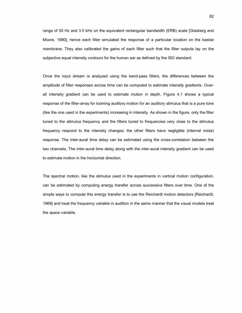
82

range of 50 Hz and 3.5 kHz on the equivalent rectangular bandwidth (ERB) scale [Glasberg and

Moore, 1990]; hence each filter simulated the response of a particular location on the basilar

membrane. They also calibrated the gains of each filter such that the filter outputs lay on the

subjective equal intensity contours for the human ear as defined by the ISO standard.

Once the input stream is analyzed using the band-pass filters, the differences between the

amplitude of filter responses across time can be computed to estimate intensity gradients. Over-

all intensity gradient can be used to estimate motion in depth. Figure 4.1 shows a typical

response of the filter-array for looming auditory motion for an auditory stimulus that is a pure tone

(like the one used in the experiments) increasing in intensity. As shown in the figure, only the filter

tuned to the stimulus frequency and the filters tuned to frequencies very close to the stimulus

frequency respond to the intensity changes; the other filters have negligible (internal noise)

response. The inter-aural time delay can be estimated using the cross-correlation between the

two channels. The inter-aural time delay along with the inter-aural intensity gradient can be used

to estimate motion in the horizontal direction.

The spectral motion, like the stimulus used in the experiments in vertical motion configuration,

can be estimated by computing energy transfer across successive filters over time. One of the

simple ways to compute this energy transfer is to use the Reichardt motion detectors [Reichardt,

1969] and treat the frequency variable in audition in the same manner that the visual models treat

the space variable.

83

Figure 4.1: Typical filter response to looming auditory motion

4.1.2. Visual Motion Processing

Numerous models have been developed for the various stages of visual motion perception.

Reichardt’s correlation model [Reichardt, 1969] was the first successful model and its variations

are still in use [Van Santen and Sperling, 1985]. Adelson & Bergen [1985] developed a two-stage

model for computing visual motion, which was later, used by Qian, Anderson and Adelson [1994]

to model the perception of transparent motion. The first stage uses spatiotemporal Gabor filters to

compute local motion energy. The spatiotemporal filters are phase-sensitive, i.e., their response

is dependent on how the motion vectors align with their receptive fields. Adelson and Bergen

used quadrature pairs of Gabor filters, one with an even phase and the other with an odd phase,

and added the square of the output of each filter in the pair to compute motion energy in a given

direction. Therefore, if f(x,y,t) is the mathematical function that defines certain motion sequence

84

and ge(f,t,�) and go(f,t,�) are the Gabor filters with even and odd phase, respectively, as a

function of spatial frequency f, time t and orientation �. Then the motion energy along any

direction � can be computed by,

E = [f * ge]2 + [f * go]2 … (4.1)

The values of f and � can be varied for calculating motion energies for different spatial

frequencies and along different directions. This stage has minimal lateral interaction and

corresponds to V1 neurons. The second stage is the pooling stage, which takes input from

multiple filters and integrates them together. This stage corresponds to the MT neurons and

shows a strong inhibition for opposite directions of motion. Figure 4.2 shows the schematic of the

model developed by Adelson & Bergen. Hong [2005] successfully extracted visual motion from a

random-dot pattern using this approach.

Figure 4.2: Adelson & Bergen two-stage motion model

4.2. Biased-Competition Model

2

Space

Time

2 2 2

85

A B

The current model simulated the crossmodal interactions by considering inhibitory and excitatory

feed-forward connections from lower level unimodal areas to higher integrative multimodal

neurons as well as feedback connections going in the other directions. The excitatory and

inhibitory interactions were modeled adapted from the biased-competition hypothesis first

proposed by Desimone and Duncan [1995] and later implemented by Reynolds et al. [1999] in a

simple feed-forward neural network model.

Desimone and Duncan [1995] argued that visual cortical areas have a limited capacity to process

information and only a fraction of the information that reaches the retina is processed at any point

in time. The perceptual objects compete for resources in these visual areas. In order to deal with

this limited capacity, the human visual system uses additional knowledge such as attention,

relevance to task at hand etc. to bias the competition in favor of the relevant or attended task.

Figure 4.3: Feed-forward neural network model proposed by Reynolds et al. [1999]

Reynolds et al. [1999] used this hypothesis to develop a competitive neural network. Figure 4.3

shows the schematic of the model. Let us assume that both the vertical target (object A) and

86

horizontal target (object B) in the visual field are competing for the resources of the neuron

depicted by the top circle in the figure. Its firing rate is denoted by the letter y. Let us further

assume that there are two neurons (depicted by the bottom two circles) that are tuned to vertical

and horizontal orientation with firing rates denoted by x1 and x2 respectively. Each of those two

neurons has an excitatory as well as inhibitory input to the neuron Y, weighted by factors wi+ and

wi- (i = 1,2), respectively. Then, according to Reynolds et al. [1999] the total excitatory input to

neuron Y is given by,

E = w1+ x1 + w2

+ x2 … (4.2)

and the total inhibitory input is given by,

I = w1- x1 + w2

- x2 … (4.3)

The equation below describes the firing rate of the neuron Y,

dydt

= (B - y )E - yI - Ay … (4.4)

In the above equation B is the maximum firing rate of the neuron and A is the passive decay rate

of the neuron. This equation was first proposed by Grossberg [1973] to explain how feed-forward

networks can be designed whose response to high-energy input (for example, high luminance

stimulus) does not saturate while at the same time the network is sensitive to low energy inputs.

In the limiting case, as t Æ � , the final output of the neuron is given by,

tÆ�y = EB

E + I + A … (4.5)

87

Since B and A are both constants (properties of the neuron), the firing rate is dependent on the

excitatory input E and inhibitory input I to the neuron, which can be controlled (or biased) by the

weight factors wi+ and wi

- (i = 1,2). The inhibitory and excitatory connections between unimodal

neurons and multimodal neurons were modeled in a similar fashion and the connections weights

were used as the model parameters.

4.3. Computational model for crossmodal interactions between auditory

and visual motion mechanisms

In the current study, I developed a model with three different configurations based on the same

principles but slightly different model structure and parameters to simulate crossmodal

interactions for the three motion configurations described in Chapter 2, namely, horizontal motion

configuration, vertical motion configuration and motion-in-depth configuration. For each motion

configuration, I modeled both short-term crossmodal motion interactions, when motion stimuli are

presented simultaneously in both the modalities, as well as long-term crossmodal interactions,

the crossmodal motion aftereffects (MAE). The same model parameters were used to simulate

results for both influence types (auditory-to-visual and visual-to-auditory) for each motion

configurations. The following three sections cover the specific details of the three motion

configurations: horizontal motion configuration, vertical motion configuration and motion-in-depth

configuration.

4.4. Computation Model for Horizontal Motion Configuration

Figure 4.4 shows the multi-sensory interactions for horizontal motion configuration. I considered

auditory and visual neurons tuned to leftward and rightward motion. These neurons are shown as

88

AL, AR, VL and VR, respectively, in the figure. These neurons provide input to the multi-sensory

superior colliculus (SC) neurons shown as SCL and SCR in the figure. I hypothesize that this

multimodal site is the superior colliculus (SC) because of three reasons. First, it receives input

from the visual, the auditory and the haptic modality [Meredith and Stein, 1986]. Second, the

receptive fields of these modalities are topographically mapped in the area SC [Meredith and

Stein, 1996]. Third, the neurons in area SC also provide input to pre-motor areas that mediate

general attentive and orienting behavior in humans. The subscripts ‘L’ and ‘R’ denote leftward

and rightward motion, respectively. The inhibitory connections are shown with red dashed arrows

and circles, while the excitatory connections are shown with green plain solid arrows. Each

double-headed arrow actually represents two neural connections, one in each of the opposite

directions; only one line was used for simplicity. Thus, there are two weights associated with each

line that control the interactions to and from the two neurons that it connects. The multimodal SC

neurons receive excitatory input from the unimodal neurons tuned to the same direction and

receive inhibitory input from unimodal neurons tuned to opposite direction. The SC neurons, in

turn, modulate the activity of the unimodal neurons through excitatory/inhibitory feedback

connections to unimodal neurons tuned to same/opposite directions of motion.

89

Figure 4.4: Cross-modal interactions model for leftward/rightward motion. The red dashed arrows with circles denote inhibitory connections while the green plain solid arrows denote excitatory connections. Each of these connections is modulated by an associated weight, used as a model parameter.

In the current model, it was assumed that the weight for an inhibitory connection from a unimodal

neuron to a multimodal neuron tuned to opposite direction of motion is equal to the weight of the

90

excitatory connection from the unimodal neuron to multimodal neuron tuned to the same direction

of motion. Table 4.1 provides the definition of each of the weights shown in the figure.

Model

Parameter Model Parameter Definition

WA Mutual inhibition weight for connection between two auditory neurons tuned

to opposite direction of motion

WV Mutual inhibition weight for connection between two visual neurons tuned to

opposite direction of motion

WAM Excitatory/inhibitory connection weight from auditory neuron to multimodal

neuron tuned to same/opposite direction of motion

WMA Excitatory/inhibitory connection weight from multimodal neuron to auditory


WVM Excitatory/inhibitory connection weight from visual neuron to multimodal


WMV Excitatory/inhibitory connection weight from multimodal neuron to visual


Table 4.1: Definitions of weights used as the model parameters in the crossmodal interactions model

The firing rate of each of the neurons considered in the model is determined by the general

equation (4.4) described above. As an example let us consider the visual neuron tuned to

91

rightward motion. The excitatory input to VR comes from the low-level visual areas tuned to

rightward visual motion denoted by VRin

in equation (4.6) and SC neurons tuned to rightward

motion (SCR),

EVR

= VRin+ wmv (SCR - b) / SCR

max … (4.6)

The inhibitory input to VR comes from the visual neurons tuned to leftward motion (VL) and SC

neurons tuned to leftward motion (SCL),

IVR

= wv (VL - b) /VLmax + wmv (SCL - b) / SCL

max … (4.7)

Therefore, according to equation 4.4, the firing rate of neuron VR is given by,

dVR

dt= (VR

max - VR ) * EVR- VR * IVR

- DVR*VR … (4.8)

dVR

dt= [(VR

max - VR ) * {VRin+ wmv (SCR - b) / SCR

max } -

VR * {wv (VL - b) /VLmax + wmv (SCL - b) / SCL

max } -

DVR* (VR - b)] /VR

max

… (4.8a)

In the above two equations,

VRmax , SCR

max , VLmax , SCL

max the respective maximum firing rates which were taken

to be 300 spikes/second for all neurons during simulation.

b the baseline firing rate, (30 spikes/second for all neurons).

92

VR , SCR , VL , SCL the respective current firing rate for the neurons.

DVR

the passive decay for neuron VR, taken as 0.6 for all neurons

Similarly, the firing rate for neurons VL , AL ,AR , SCR , SCL are given by equations 4.9, 4.10, 4.11,

4.12, 4.13 respectively. In all of the equations below, the symbols are defined using the same

conventions as in equation 4.8a.

dVL

dt= [(VL

max - VL ) * {VLin+ wmv (SCL - b) / SCL

max } -

VL * {wv (VR - b) /VRmax + wmv (SCR - b) / SCR

max } - DVL* (VL - b)] /VL

max… (4.9)

dAL

dt= [(AL

max - AL ) * {ALin+ wma(SCL - b) / SCL

max } -

AL * {wa(AR - b) / ARmax + wma(SCR - b) / SCR

max } - DAL* (AL - b)] / AL

max… (4.10)

dAR

dt= [(AR

max - AR ) * {ARin+ wma(SCR - b) / SCR

max } -

AR * {wa(AL - b) / ALmax + wma(SCL - b) / SCL

max } - DAR* (AR - b)] / AR

max… (4.11)

dSCR

dt= [(SCR

max - SCR ) * {wam(AR - b) / ARmax + wvm(VR - b) /VR

max } -

SCR * {wam(AL - b) / ALmax + wvm(VL - b) /VL

max } - DSCR* (SCR - b)] / SCR

max… (4.12)

dSCL

dt= [(SCL

max - SCL ) * {wam(AL - b) / ALmax + wvm(VL - b) /VL

max } -

SCL * {wam(AR - b) / ARmax + wvm(VR - b) /VR

max } - DSCL* (SCL - b)] / SCL

max… (4.13)

4.4.1. Simulation results – Transient crossmodal effects

93

The neural network described above was used to simulate both short-term crossmodal effects

and motion aftereffects. In all the simulations the maximum firing rate and the baseline-firing rate

were set to be 300 spikes/second and 30 spikes/second respectively for all the neurons. Further,

the passive decay constant was set to be 0.6 for all neurons before adaptation and varied it

according to the strength of adaptation to simulate MAE.

The simulations on the model were run under four different input conditions (two primary

modalities x two motion directions) to obtain the psychometric functions similar to those obtained

in Experiment 1a in Chapter 2. Tables 4.2 and 4.3 show the inputs to the model under the four

conditions and the values of the model parameters used to simulate results for the horizontal

motion configuration.

Primary Motion Secondary Motion

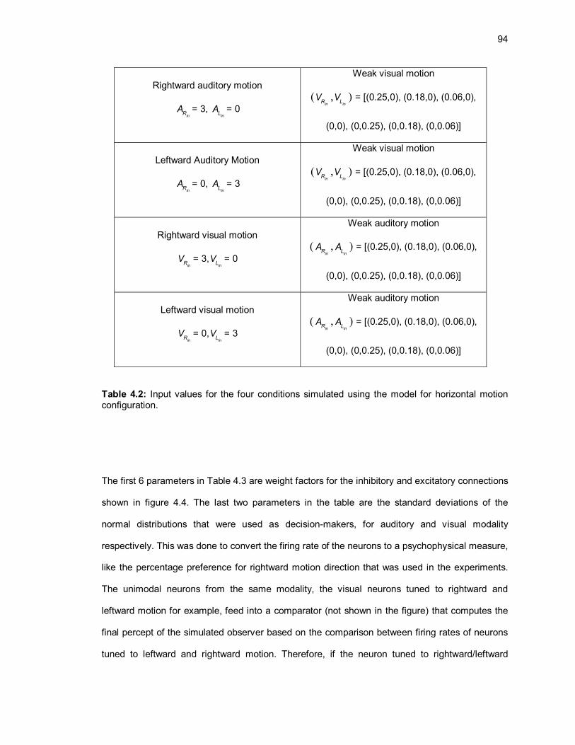
94

Rightward auditory motion

ARin

= 3, ALin

= 0

Weak visual motion

( VRin

, VLin

) = [(0.25,0), (0.18,0), (0.06,0),

(0,0), (0,0.25), (0,0.18), (0,0.06)]

Leftward Auditory Motion

ARin

= 0, ALin

= 3

Weak visual motion

( VRin

, VLin

) = [(0.25,0), (0.18,0), (0.06,0),

(0,0), (0,0.25), (0,0.18), (0,0.06)]

Rightward visual motion

VRin

= 3, VLin

= 0

Weak auditory motion

( ARin

, ALin

) = [(0.25,0), (0.18,0), (0.06,0),

(0,0), (0,0.25), (0,0.18), (0,0.06)]

Leftward visual motion

VRin

= 0, VLin

= 3

Weak auditory motion

( ARin

, ALin

) = [(0.25,0), (0.18,0), (0.06,0),

(0,0), (0,0.25), (0,0.18), (0,0.06)]

Table 4.2: Input values for the four conditions simulated using the model for horizontal motion configuration.

The first 6 parameters in Table 4.3 are weight factors for the inhibitory and excitatory connections

shown in figure 4.4. The last two parameters in the table are the standard deviations of the

normal distributions that were used as decision-makers, for auditory and visual modality

respectively. This was done to convert the firing rate of the neurons to a psychophysical measure,

like the percentage preference for rightward motion direction that was used in the experiments.

The unimodal neurons from the same modality, the visual neurons tuned to rightward and

leftward motion for example, feed into a comparator (not shown in the figure) that computes the

final percept of the simulated observer based on the comparison between firing rates of neurons

tuned to leftward and rightward motion. Therefore, if the neuron tuned to rightward/leftward

95

motion is firing very strongly compared to the neuron tuned to leftward/rightward motion, then the

comparator would give a strong preference for rightward/leftward motion as output; if the

rightward and leftward tuned neurons are firing equally strongly, then the comparator gives a

chance-level performance, thus mimicking human behavior. To incorporate internal perceptual

noise in the simulations, I ran ten simulations for each input condition adding independent

normally distributed noise to each of the parameters and inputs. The results were plotted after

averaging across simulations. I chose to run only ten simulations, since the model took a long

time to converge owing to its multiple feedback connections. Furthermore, even with only ten

simulations the standard errors measured very small which suggests that the current model is

very robust to perturbation in model parameters.

WA WV WAM WMA WVM WMV ��A ��V

0.6 0.6 0.19 0.26 0.053 0.13 43.67 66.69

Table 4.3: The values of the model parameters used to simulate results for horizontal motion configuration in Experiment 1a (attend to motion in the secondary modality).

Figure 4.5(a) and (b) show the model simulation results with auditory and vision as primary

modality respectively. The Pearson's linear correlation coefficient was 99.76 % between the data

obtained from human subjects and the data obtained from model simulations. In the subsequent

sections, Pearson's linear correlation coefficient is stated simply as correlation to provide for

better reading.

96

Figure 4.5: Simulation results for crossmodal transient effects in horizontal motion configuration when subjects attended to the secondary the modality. Primary Modality: (a) Audition (b) Vision

97

When subjects attended to both the modalities there was a stronger crossmodal effect, both when

auditory was the primary modality as well as when vision was the primary modality. This increase

in the observed crossmodal effect is reflected in the general increase in the values of crossmodal

parameters (WAM, WMA, WVM, WMV) in the model. Table 4.4 shows the parameter values used in

the simulation. It should be noted that, the values of ��A as well as �V increased drastically. This is

because subjects were less sensitive to changes in the motion strength of the secondary modality

when they attended to motion in both modalities. This is reflected in the shallow slopes of the

psychometric functions (Figure 4.6). There was a larger interference across the modalities when

subjects attended both modalities than when they ignored the primary modality completely. This

decrease in sensitivity was captured by increasing the variance of the normal distribution used by

the comparator.

WA WV WAM WMA WVM WMV �A �V

0.6 0.6 0.21 0.9 0.2 0.36 167.25 144.55

Table 4.4: The values of the model parameters used to simulate results for horizontal motion configuration in Experiment 1b (attend to motion in both modalities).

The simulations were run with the same input values as defined in Table 4.2, with the exception

of the highest strength of motion (0.25) used in the secondary modality. Thus, the simulation was

run for five signal strengths for each combination of primary modality and primary modality motion

direction. Figure 4.6(a) and (b) show the model simulation results with auditory and vision as

primary modality, respectively. There was 98.17 % correlation between the data obtained from

human subjects and the data obtained from model simulations.

98

Figure 4.6: Simulation results for crossmodal transient effects in horizontal motion configuration when subjects attended to both the modalities. Primary Modality: (a) Audition (b) Vision

99

4.4.2. Simulation Results – Crossmodal Motion Aftereffects

The experimental results showed auditory motion aftereffects (MAE) following visual adaptation

for all the three motion configurations, however, visual motion aftereffects were found only for

spectral auditory motion (vertical motion configuration). No visual MAE was observed following

adaptation to auditory spatial motion.

Repetition-suppression phenomenon refers to the reduction in the neural activity in response to

exposure to a repeated stimulus (adaptation). The MAE is one special case of repetition-

suppression phenomenon. There have been various models to explain this phenomenon with

neural fatigue model being the most commonly referred [Grill-Spector, Henson and Martin 2006

for a review]. According to the fatigue model, the reduction in the neuronal activity to a given

stimulus is proportional to the initial activity shown by the neuron to the same stimulus. Thus,

there is an overall reduction in the activity of a population of neurons to a stimulus that respond

with varying activity to the same stimulus initially.

The fatigue model was used to simulate the crossmodal MAE observed in the experiments. I

modeled the reduction in activity by reducing the maximum firing rate of the adapted neuron with

the reduction being proportional to the initial firing rate during adaptation. Secondly, I also

increased the passive decay factor of the adapted neuron, which led to a reduced response to

motion in the same direction. It should be noted that the maximum firing rate and the passive

decay parameter of the secondary modality were affected after adaptation to motion in the

primary modality. However, since I varied the effect as a function of the initial firing rate of the

neuron in response to the adapting stimulus, the effect was not as strong as the effect on the

maximum firing rate and passive decay parameter in the primary modality. Thus, the model would

lead to stronger unimodal MAE, in agreement with the findings of Kitagawa and Ichihara [2002].

They found that crossmodal auditory loudness aftereffects following adaptation to visual motion in

depth were weaker than auditory loudness aftereffects observed after adaptation to a sound

stimulus changing in loudness. I did not explicitly measure or simulate unimodal motion

100

aftereffects. Furthermore, I was able to model the observed asymmetry in crossmodal

aftereffects, the lack of crossmodal visual aftereffects following adaptation to auditory spatial

motion, by varying the model parameters that controlled the reduction in the maximum firing rate

and increase in the passive decay rate. Equation 4.14 shows the mathematical equation used to

modulate the passive decay parameter in the secondary modality following adaptation to motion

in the primary modality.

Dpa = wdDie(Ff - b)/Fmax , Ff > b

Di , Ff £ b

ÏÌÔÔÔ

ÓÔÔÔ

… (4.14)

Where,

Dpa the post-adaptation decay parameter

Di the pre-adaptation decay parameter

Ff the firing rate in response to the adaptation stimulus

Fmax the pre-adaptation maximum firing rate

b the baseline firing rate of the neuron

wd the model parameter to modulate the effect of adaptation on the passive decay

parameter. Shown as wavd ,wvad during simulation when the primary modality is

audition and vision, respectively.

Equation 4.15 gives the mathematical formula for modulating the maximum firing rate in the

secondary modality due to adaptation to motion in the primary modality.

Fmaxpa = wf Fmaxe

- (Ff - b)/Fmax , Ff > b Fmax , Ff £ b

ÏÌÔÔÔ

ÓÔÔÔ

… (4.15)

101

Where,

Fmaxpa the post-adaptation maximum firing rate

Ff the firing rate in response to the adaptation stimulus

Fmax the pre-adaptation maximum firing rate

b the baseline firing rate of the neuron

wf the model parameter to modulate the effect of adaptation on the maximum firing

rate. Shown as wavf ,wvaf during simulation when the primary modality is audition

and vision, respectively.

The simulation was run in two parts similar to the trials in the actual experiment. First, the

response of each neuron to the adaptation stimulus was determined and then the values obtained

were used to determine the new passive decay parameter and maximum firing rate for each

neuron. In the second part, the response to the test stimulus was determined following

adaptation, with the new values of passive decay parameter and maximum firing rate obtained in

the previous step. The connection weight factors used in these simulations were the same as the

ones obtained in Experiment 1a, since subjects always attended to motion in a single modality at

a time both in Experiment 1a and in the adaptation experiments.

Similar to the simulations for the crossmodal transient effect condition, I repeated the simulation

ten times for each input condition adding independent normally distributed noise to each of the

parameters and inputs. The results were plotted after averaging across simulations. Tables 4.5

and 4.6 show the parameter values used for simulating unimodal and bimodal adaptation

conditions, respectively. The results obtained were very similar for the two adaptation conditions;

in other words, the presence of an ambiguous motion signal in the secondary modality had very

little effect on the strength of the crossmodal motion aftereffects. This fact is reflected in the very

similar parameter values used to simulate results for both the adaptation conditions. The input

values were the same as the ones described in Table 4.2, however the primary modality and

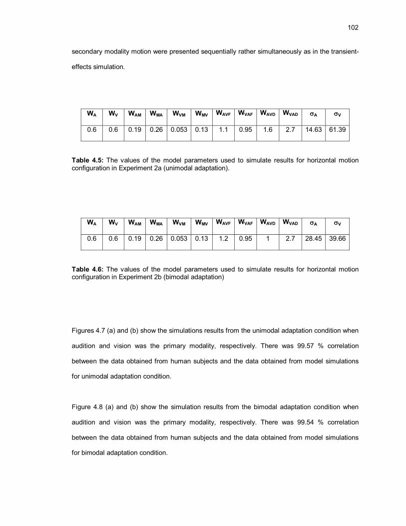
102

secondary modality motion were presented sequentially rather simultaneously as in the transient-

effects simulation.

WA WV WAM WMA WVM WMV WAVF WVAF WAVD WVAD ��A ��V

0.6 0.6 0.19 0.26 0.053 0.13 1.1 0.95 1.6 2.7 14.63 61.39

Table 4.5: The values of the model parameters used to simulate results for horizontal motion configuration in Experiment 2a (unimodal adaptation).


0.6 0.6 0.19 0.26 0.053 0.13 1.2 0.95 1 2.7 28.45 39.66

Table 4.6: The values of the model parameters used to simulate results for horizontal motion configuration in Experiment 2b (bimodal adaptation)

Figures 4.7 (a) and (b) show the simulations results from the unimodal adaptation condition when

audition and vision was the primary modality, respectively. There was 99.57 % correlation

between the data obtained from human subjects and the data obtained from model simulations

for unimodal adaptation condition.

Figure 4.8 (a) and (b) show the simulation results from the bimodal adaptation condition when

audition and vision was the primary modality, respectively. There was 99.54 % correlation

between the data obtained from human subjects and the data obtained from model simulations

for bimodal adaptation condition.

103

Figure 4.7: Simulation results for crossmodal MAE in horizontal motion configuration when subjects adapted unimodally. Primary Modality: (a) Audition (b) Vision

104

Figure 4.8: Simulation results for crossmodal MAE in horizontal motion configuration when subjects adapted bimodally. Primary Modality: (a) Audition (b) Vision

105

4.5. Computation Model for Vertical Motion Configuration

Figure 4.9 shows the multi-sensory interactions for vertical motion configuration. The model

structure is analogous to the one developed for horizontal motion configuration. I considered

visual neurons tuned to upward and downward spatial motion and auditory neurons tuned to

upward and downward spectral motion. These neurons are shown as AU, AD, VU and VD,

respectively in the figure. These neurons provide input to the multi-sensory SC neurons shown as

SCU and SCD in the figure. The subscripts ‘U’ and ‘D’ denote upward and downward motion

respectively. Similar to figure 4.4, the inhibitory connections are shown with red dashed arrows

and circles, while the excitatory connections are shown with plain green solid arrows. Each

double- headed arrow has two weights associated with it that control the interactions to and from

the two neurons that it connects. The crossmodal connections considered were similar to the

ones considered for horizontal motion configuration: The multimodal SC neurons receive

excitatory input from the unimodal neurons tuned to the same direction and receive inhibitory

input from unimodal neurons tuned to opposite direction. The SC neurons, in turn, modulate the

activity of the unimodal neurons through excitatory/inhibitory feedback connections to unimodal

neurons tuned to same/opposite directions of motion. The model weight factors have the same

definition as defined in Table 4.1 and the governing equations were derived in a similar fashion as

equations 4.8 – 4.13.

Similar to the simulations for horizontal motion configuration, the maximum firing rate and the

baseline-firing rate were fixed to be 300 spikes/second and 30 spikes/second respectively for all

the neurons during simulation. I further fixed the passive decay constant to be 0.6 for all neurons

before adaptation, and varied it according to the strength of adaptation to simulate MAE. The

simulations were repeated ten times with independent random noise added to each parameter to

simulate the variance in human behavior. The input conditions were analogous to the conditions

defined in Table 4.2. Hence, there were four conditions (upward/downward primary modality

direction x vision/audition primary modality) for which the psychometric functions were obtained.

106

Figure 4.9: Cross-modal interactions model for vertical motion configuration. The red dashed arrows with circles denote inhibitory connections while the green plain solid arrows denote excitatory connections. Each of these connections is modulated by an associated weight, which was used as a model parameter.

107

4.5.1 Simulation Results – Transient Effects

Tables 4.7 and 4.8 show the parameter values used for simulation of the two attentional

conditions: attend secondary modality and attend both modalities, respectively. The two

attentional conditions led to very similar results and hence very similar weight factors for the

model simulations. It should be noted that similar to the results obtained in the horizontal motion

configuration, subjects were less sensitive (��A and �V values were larger) to motion strength in

the secondary modality when the task involved attending to motion in both modalities.


0.5 0.5 0.2 0.125 0.125 0.25 35.75 74.86

Table 4.7: The values of the model parameters used to simulate results for vertical motion configuration in Experiment 1a (attend to motion in the secondary modality).

Figures 4.10 (a) and (b) show the simulation results from “attend to motion in the secondary

modality” experiment, when audition and vision was the primary modality, respectively. There was

99.64 % correlation between the data obtained from human subjects and the data obtained from

model simulations. Figures 4.11 (a) and (b) show the simulation results from “attend to motion in

both modalities” experiment when audition and vision was the primary modality, respectively.

There was 99.17 % correlation between the data obtained from human subjects and the data

obtained from model simulations.


0.5 0.5 0.2 0.125 0.125 0.25 43.14 93.38

Table 4.8: The values of the model parameters used to simulate results for vertical motion configuration in Experiment 1b (attend to motion in both modalities).

108

Figure 4.10: Simulation results for crossmodal transient effects in vertical motion configuration when subjects attended to the secondary modality. Primary Modality: (a) Audition (b) Vision

109

Figure 4.11: Simulation results for crossmodal transient effects in vertical motion configuration when subjects attended to both the modalities. Primary Modality: (a) Audition (b) Vision

110


The simulations for vertical motion configurations were run in the same way as the simulations for

horizontal motion configuration described in the pervious section. Table 4.9 shows the parameter

values used during simulation of crossmodal MAE in the vertical motion configuration for the

unimodal adaptation condition. Figures 4.12 (a) and (b) show the results from the simulations

when audition and vision were the primary modality, respectively. There was a 99.57% correlation

between the data obtained from human subjects and the data obtained from model simulation.


0.5 0.5 0.2 0.125 0.125 0.25 1 0.95 0.6 1.5 22.13 111.99

Table 4.9: The values of the model parameters used to simulate results for vertical motion configuration in Experiment 2a (unimodal adaptation).

Table 4.10 shows the parameter values used during simulation of crossmodal MAE in the vertical

motion configuration for the bimodal adaptation condition. Figures 4.13 (a) and (b) show the

results from the simulations when audition and vision were the primary modality, respectively.

There was a 99.84% correlation between the data obtained from human subjects and the data

obtained from model simulation.


0.5 0.5 0.2 0.125 0.125 0.25 1 0.95 0.6 1.5 37.41 9.99

Table 4.10: The values of the model parameters used to simulate results for vertical motion configuration in Experiment 2a (bimodal adaptation).

111

Figure 4.12: Simulation results for crossmodal MAE in vertical motion configuration when subjects adapted unimodally. Primary Modality: (a) Audition (b) Vision

112

Figure 4.13: Simulation results for crossmodal MAE in vertical motion configuration when subjects adapted bimodally. Primary Modality: (a) Audition (b) Vision

113

4.6. Computation Model for Motion-in-depth Configuration

Figure 4.14 shows the crossmodal interactions considered for motion-in-depth configuration.

Along with the auditory and visual neurons tuned to motion in depth, i.e. approach (A) and recede

(W), I also considered auditory neurons that are tuned to stimulus that do not move in depth,

depicted by AN in the figure. There was mutual inhibition between AN and auditory neurons tuned

to motion in depth as well as multimodal neurons tuned to motion in depth, both approaching and

receding.

The visual stimulus used in the experiments was in fact bistable: it could either be perceived as

approaching/receding or as expanding/contracting in the same fronto-parallel plane. The reason

for that is that the stimulus did not alter in size, which is a strong cue for motion in depth. Also,

there was no radial acceleration or deceleration as the gratings expanded or contracted to

provide a close resemblance to an object moving in depth. It has been shown that an

accompanying auditory stimulus changing in loudness can alter the perception of random dots

moving radially outwards. Masuda, Wada, Kitagawa and Noguchi [2002] showed that subjects

perceived random dots moving radially outwards as looming or as expanding in the same plane

when they were accompanied by a sound increasing or decreasing in loudness respectively. In

the bimodal adaptation MAE experiment and to some extent in the transient effect experiment

when subjects attended to both modalities, it is possible that the presence of an ambiguous or

weak motion in depth signal in the auditory modality would have influenced the percept of visual

motion in depth stimulus.

To simulate these effects, I also incorporated an auditory neuron that responds to fixed depth

stimulus. Furthermore, to incorporate the fact that the visual stimulus used was relatively weaker;

the visual input was set to be 2 units (instead of 3 units as in simulations for horizontal and

vertical motion configurations, Table 4.2) when vision was the primary modality. The governing

equations for the simulations were derived in the same way as for simulations for horizontal and

114

vertical motion configurations. The maximum firing rate and the baseline-firing rate were fixed at

300 spikes/second and 30 spikes/second respectively, for all the neurons.

Figure 4.14: Cross-modal interactions model for motion-in-depth configuration. The red dashed arrows with circles denote inhibitory connections while the green plain solid arrows denote excitatory connections. Each of the connections was modulated by an associated weight, which was then used as a model parameter.

115

4.6.1. Simulation Results – Transient Crossmodal Effects

Table 4.11 shows the model parameters used for simulating the experimental results for motion-

in-depth configuration when subjects attended to motion only in the secondary modality. Figures

4.15 (a) and (b) show the results for model simulation for the same condition. There was a

correlation of 98.46 % between data obtained from human subjects and data obtained from

model simulations.

WN WA WV WANM WMAN WAM WMA WVM WMV ��A ��V

0.5 0.6 0.6 0.18 0.2 0.2 0.18 0.21 0.18 46.52 113.61

Table 4.11: The values of the model parameters used to simulate results for motion-in-depth configuration in Experiment 1a (attend to motion in the secondary modality).

Table 4.12 shows the model parameters used for simulating the experimental results for motion-

in-depth configuration when subjects attended to motion in both the modalities. Figures 4.16 (a)

and (b) show the results for model simulation for the same condition. There was a correlation of

99.26 % between data obtained from human subjects and data obtained from model simulations.

The bistable nature of the visual stimulus is also reflected in the low sensitivity in the visual

motion discrimination task as shown by the relatively large values of ��V in both attentional

conditions. As expected, �A is larger when subjects attended to motion in both modalities, which

in turn led to more interference across modalities.

WN WA WV WANM WMAN WAM WMA WVM WMV �A �V

0.5 0.6 0.6 0.18 0.2 0.2 0.18 0.21 0.18 90.29 101.44

Table 4.12: The values of the model parameters used to simulate results for motion-in-depth configuration in Experiment 1b (attend to motion in both the modalities).

116

Figure 4.15: Simulation results for crossmodal transient effects in motion-in-depth configuration when subjects attended to the secondary modality. Primary Modality: (a) Audition (b) Vision

117

Figure 4.16: Simulation results for crossmodal transient effects in motion-in-depth configuration when subjects attended to both the modalities. Primary Modality: (a) Audition (b) Vision

118


Table 4.13 gives the model parameters used for simulating experimental results for crossmodal

motion aftereffects in motion-in-depth configurations when subjects adapted to a unimodal motion

signal in the primary modality. Figures 4.17 (a) and (b) show the results of the simulation from the

same condition. There was a correlation of 99.05% between data obtained from human subjects

and data obtained from model simulations.

WAVF WVAF WAVD WVAD ��A ��V

1 0.9 0.6 1.7 31.61 103.37

Table 4.13: The values of the model parameters used to simulate results for vertical motion configuration in Experiment 2a (unimodal adaptation). WN, WA, WV, WANM, WMAN, WAM, WMA, WVM and WMV have the same values as defined in Table 4.12.

Table 4.14 shows the model parameters when subjects adapted to bimodal motion signal in the

motion-in-depth configuration. Figures 4.18 (a) and (b) show the simulation results when audition

and vision were the primary modality, respectively. There was a correlation of 99.78% between

data obtained from human subjects and data obtained from model simulation.

WAVF WVAF WAVD WVAD ��A ��V

1 0.9 0.6 1.7 17.55 24.35

Table 4.14: The values of the model parameters used to simulate results for vertical motion configuration in Experiment 2b (bimodal adaptation). WN, WA, WV, WANM, WMAN, WAM, WMA, WVM and WMV have the same values as defined in Table 4.12.

119

Figure 4.17: Simulation results for crossmodal MAE in motion-in-depth configuration when subjects adapted unimodally. Primary Modality: (a) Audition (b) Vision

120

Figure 4.18: Simulation results for crossmodal MAE in motion-in-depth configuration when subjects adapted bimodally. Primary Modality: (a) Audition (b) Vision

121

4.7. Computational model for attentional modulation of motion aftereffects

within the auditory and the visual modality

This section describes the computational model that was developed to provide a possible

explanation for the observed effect of spectral attention on motion aftereffects within the auditory

and the visual modality in the experiments presented in Chapter 3 of the thesis. I designed the

model based on the principles of the biased-competition model presented in section 4.2. I

modeled the effect of attention by modulating the weights of neuronal connections in favor of the

attended spectral features. The same model structure was used to explain the attentional effect in

both the auditory and the visual modality. The models are based on Cunningham’s [2008]

argument that attention acts in a similar fashion in the auditory and the visual modality.

4.7.1. Computational model for the role of spectral attention within visual/auditory motion

processing

Figure 4.19 shows the model architecture for the effect of spectral attention on visual/auditory

motion processing. The model is presented in terms of visual motion processing for simplicity. An

analogous model was used for auditory motion processing. The neurons HFR and HFL denote the

lower level directional neurons, in the visual are V1 that are narrowly tuned to high spatial

frequencies moving rightwards and leftwards, respectively. LFR and LFL denote analogous

neurons tuned to low spatial frequencies. Neurons tuned to medium spatial frequencies were not

considered in the simulations because medium spatial frequencies were never in the adapting

stimuli. These neurons provide input to the integrative MT subunits that pool local motion energy

across broader ranges of spatial frequencies with different weights assigned to motion around

different spatial frequencies. MHFR, MMFR and MLFR denote the MT subunits broadly tuned to

high, medium and low spatial frequencies moving rightwards and MHFL, MMFL and MLFL denote

corresponding neurons tuned to leftward motion. The lower-level neurons provide excitatory input

to the MT neurons tuned to the same direction of motion and inhibitory input to the MT neurons

tuned to the opposite direction of motion. The MT neurons tuned to the same direction of motion

122

mutually excite each other. The model for auditory motion processing is exactly the same,

however, the neurons were tuned to temporal frequency rather than spatial frequency as in the

case of the visual motion processing. Table 4.15 defines the model parameters used in the

simulations.

Figure 4.19. Spectral attention model for visual/auditory motion processing. The red dashed arrows with circles denote inhibitory connections while the green plain solid arrows denote excitatory connections. Each of the connections was modulated by an associated weight, which was then used as a model parameter.

123

Model

Parameter Model Parameter Definition

WM Mutual excitatory weight for connection between higher integrative neurons

tuned to same direction of motion

WS Excitatory/Inhibitory weight for input from lower-level neurons to higher level

neurons tuned to similar spatial frequencies in the same/opposite direction

WD

Excitatory/Inhibitory weight for input from lower-level neurons to higher level

neurons tuned to neighboring spatial frequencies in the same/opposite

direction

Table 4.15: Definitions of weights used as the model parameters in the spectral attention model

4.7.2. Simulation results

The governing equations for the firing rate of all the neurons in the model described above were

determined using equation 4.4 described in section 4.2. In all the simulations the maximum firing

rate and the baseline-firing rate were fixed to be 300 spikes/second and 30 spikes/second

respectively for all the neurons. Further, the passive decay constant was set to be 0.6 for all

neurons before adaptation. In the experiments described in Chapter 3, the motion aftereffect

(MAE) duration was used as a measure of the MAE strength. However, in the simulations the

increase in the passive decay constant after adaptation was used as an indicator of the strength

of the MAE. According to equation 4.14,

Dpa = wdDie

(Ff - b)/Fmax , Ff > b

124

Therefore, the MAE strength can be approximated using the following relation,

MAE Strength μ e (Ff - b)/Fmax … (4.16)

In all the simulations the relation above was used to estimate the MAE strength both in the visual

as well as the auditory modality.

In a Monte-Carlo simulation, I ran 50 trials for each of the four adaptation conditions (attend

high/low frequency moving rightwards/leftwards). For each trial, I added independent random

noise to model parameters to simulate the internal noise in the human brain. In order to compare

the simulation data with the experimental data, the same normalization was performed on the

model simulation data as on the experimental data. I normalized the MAE strength by the

average absolute mean strength measured for all conditions in a given experiment. For example,

for the auditory MAE experiment, I first found the mean MAE duration for all four conditions;

namely, attend to high frequency sound as it moves rightwards, attend to high frequency sound

as it moves leftwards, attend to low frequency sound as it moves rightwards and attend to low

frequency sound as it moves leftwards. I then computed the average of the four MAE durations

found above and then normalized each one of them by this averaged value.

Table 4.16 shows the parameter values used to simulate the effect of spectral attention effect on

motion aftereffects within the auditory modality. Von Grunau, Bertone and Pakneshan [1998]

showed that selective attention not only increases the strength of visual MAE to the attended

stimulus but also decreases the strength of visual MAE to the unattended stimulus. This effect

was simulated in the model by increasing the weights associated with attended frequency motion

and simultaneously decreasing the weights associated with unattended frequency components.

For example, when simulating “attend high frequency” condition in the auditory motion aftereffect

experiment, weights WS and WD were increased by 20% when they were associated with the high

125

frequency motion and decreased by 20% when they were associated with the low frequency

motion.

WM WS WD

0.2 0.7 0.35

Table 4.16: The values of the model parameters used to simulate results for auditory spectral attention experiment (MAE duration).

It has been argued that different mechanisms are responsible for static MAE and dynamic MAE,

given the discrepancies between their properties [Culham et al., 1998]. They also suggest that

the two aftereffects originate at separate sites within the human brain. Furthermore, in the

experiments it was found that the direction of MAE was dependent on whether the test stimulus

was dynamic or static. Namely, when static motion aftereffect was measured, the MAE direction

was consistent with high-frequency component of the adaptation stimulus and, when dynamic

motion aftereffect was measured, the MAE direction was consistent with the low-frequency

component of the adaptation stimulus. In order to account for these effects in the current model,

separate sites of origin were considered for static and dynamic MAE, with the static MAE site

having a preference for high-frequency motion, and the dynamic MAE site having a preference for

low-frequency motion. This preference was modeled by doubling the weight of the preferred

frequency motion signal. Therefore, for the static MAE site, both WS and WD for connections from

low-level neurons tuned to high frequency motion were twice in magnitude than the weights for

corresponding connections from low-level neurons tuned to low frequency motion. Tables 4.17

and 4.18 show the model parameters used to simulate the effect of spectral attention on visual

static and dynamic MAE, respectively. Similar to the auditory condition, I simulated the effect of

attention in the model by increasing the weights associated with attended frequency motion and

simultaneously decreasing the weights associated with unattended frequency components.

126

WM WS WD

0.2 0.7 0.4

Table 4.17: The values of the model parameters used to simulate results for visual spectral attention experiment (Static MAE duration).

WM WS WD

0.2 0.7 0.65

Table 4.18: The values of the model parameters used to simulate results for visual spectral attention experiment (Dynamic MAE duration).

Figures 4.20 (a) and (b) show the simulation data and the behavioral data, respectively, for the

effect of spectral attention on auditory MAE, static visual MAE and dynamic visual MAE. Figure

4.21 shows the correlation between the data obtained from the model simulation and the

behavioral data obtained from the experiments. As can be seen from the plot, the simulation data

agree very closely with the experimental data. There was a 99.63% correlation (Pearson's linear

correlation) between the data obtained from the model simulation and the behavioral data

obtained from the experiments.

127

Figure 4.20(a). Model simulation results (b) Behavioral results for the experiments on the effect of spectral attention on motion aftereffects within the auditory and the visual modalities.

a

b

128

Figure 4.21. Correlation between the data obtained from the model simulation and the behavioral data obtained from the spectral attention experiments.

129

4.8. Conclusions

I successfully developed two neurophysiologically relevant computational models to simulate and

explain the experimental findings. The first model dealt with the interactions between the auditory

and the visual motion mechanisms and the second model provided possible mechanisms to

explain the effect of spectral attention on motion processes within the auditory and the visual

modality. The crossmodal interactions across the three different motion configurations were

simulated using very similar structures. Moreover, the values of the parameters used to simulate

the crossmodal interactions were very similar across the three motion configurations. For the

second model, I used the same model architecture to explain the attentional modulation of both

auditory and visual MAE. The data obtained from the models were very well correlated, 99.32%

for crossmodal interactions model and 99.63% for spectral attention model, with the behavioral

data obtained from human subjects during the experiments. It should be noted that the current

models had a very robust structure. There was minimal variation in the simulation results when

independent random noise was added to each of the parameters. The random noise added to

each parameter during simulations was normally distributed with a variance equal to 10% of the

parameter value. When this variance was increased to 25%, the correlation (Pearson’s R)

between the model data and the behavioral data decreased to 85-90%, which suggests that the

models were reasonably robust even to large variations in the model parameters.

In the transient effect conditions of crossmodal interactions experiments, the attentional condition

did not alter the crossmodal effect, however it did affect the sensitivity of subjects in the motion

direction discrimination task. Subjects were less sensitive to the changes in motion strength in the

secondary modality when they were asked to simultaneously attend motion in both modalities.

The model parameters ��A and �V tended to be larger in the simulation of experiments when

subjects were performing a dual modality task for all the three motion configurations. This would

suggest that there is a common amodal attentional system at play, since there was a decrease in

performance (reduction in sensitivity) when subjects divided their attention between auditory and

visual modalities.

130

In the crossmodal MAE experiments simulation the ��V values tended to be smaller in bimodal

adaptation experiments compared to unimodal adaptation experiments for all the three motion

configurations. One possible explanation for this increase in sensitivity could be that subjects

were able to use the ambiguous visual motion signal present during adaptation as some sort of

reference when they performed direction discrimination task on the test stimulus, thus improving

their sensitivity. There was no such trend observed with �A, which could be because of the fact

that a monotonous pure tone at the test frequency during adaptation might have fatigued the

channels tuned to that frequency and thus nullify the advantage subjects might have gained by

using it as a reference.

In the spectral attention experiments the results showed that the effect of spectral attention was

strongest in the auditory modality (spectral attention biased the direction of the ensuing MAE).

There was a moderate effect of spectral attention on visual static MAE duration (the direction did

not reverse but the duration was significantly altered) and weakest effect of spectral attention on

visual dynamic MAE duration. This effect can be attributed to the narrow frequency tuning of the

motion mechanisms within the auditory modality (the auditory areas are tonotopically organized)

and slightly broader tuning for motion mechanisms within the visual modality. This progressively

broader frequency tuning is also reflected in the model parameters. The difference between WS

(excitatory/Inhibitory weight for input from lower-level neurons to higher-level neurons tuned to

similar spatial frequencies) and WD (excitatory/Inhibitory weight for input from lower-level neurons

to higher-level neurons tuned to neighboring spatial frequencies) was highest for the simulation of

auditory MAE experiment and weakest for the simulation of visual dynamic MAE experiment. The

current spectral attention model was also able to account for the frequency preference of the two

visual MAE mechanisms, the static MAE mechanism and the dynamic MAE mechanism, using

the same model structure. The fact that the same model architecture was able to account for the

effect to spectral attention on both the auditory and the visual motion aftereffects suggests that

attention acts in a similar fashion within the two modalities.

131

CHAPTER 5

CONCLUSIONS AND SCOPE FOR FUTURE WORK

The physical world is dynamic in nature with a multitude of events occurring simultaneously. The

human brain senses most of these events by multiple sensory modalities and integrates this

information to build a uniform and consistent representation of the event. Recently, a lot of

experiments, both neurophysiological and psychophysical, have been designed to study cross-

modal integration in general and auditory-visual interactions in particular.

The current thesis makes three significant contributions to the growing literature of auditory-visual

interactions. First, I showed that simultaneous presentation of a strong motion signal in the

auditory modality influences motion perception in the visual modality much the same way as

strong motion in the visual modality affects auditory motion perception. Furthermore, I observed

crossmodal aftereffects only when subjects adapted to spatial motion in the visual modality

(visual-to-auditory influence type) and not in the auditory modality. However, adaptation to

auditory spectral motion did induce vertical visual motion aftereffects. Second, I showed that

attention to the spectral features of one of two competing motion stimuli modulates the motion

aftereffect (MAE) in both the visual as well as the auditory modality. The results suggest that

selective attention influences motion perception in a similar fashion in both modalities. Third, I

developed a neural network model based on low-level interactions between the auditory and the

visual motion mechanisms, mediated via feedback connections from higher integrative stages

(such as the Superior Colliculus) to provide a possible mechanism for crossmodal interaction

between the auditory and the visual motion mechanisms. In addition, I developed a second model

based on the biased-competition model [Reynolds et al., 1999] to explain the effect of spectral

attention on the motion aftereffects within the auditory and the visual modalities. There was an

excellent correlation between the simulation data and the behavioral data obtained from the

132

experiments for both models, the crossmodal interaction model as well as the spectral attention

model.

5.1. Interactions between the auditory and the visual motion mechanisms

In the first experiment, I showed that simultaneously presenting a strong motion signal in one

modality (visual or auditory) with a weak motion signal in the other modality (auditory or visual)

influences the perception of the weak motion signal both when the weak motion signal is in the

auditory as well as in the visual modality. This was true for motion along the x-, y- and z-axis.

These effects were measured under two attentional conditions: one, when subjects ignored the

strong motion in the primary modality, two, when subjects attended to motion in both the

modalities. The observed effects were similar under both the attentional conditions, which

suggests that the observed crossmodal effects are not influenced by attention. The strongest

crossmodal effects were found for motion along the x-axis, the horizontal motion configuration.

This is because the auditory and visual motion stimuli had the highest degree of spatial co-

localization in the horizontal motion configuration; it has been shown that spatial co-localization is

necessary for low-level crossmodal integration [Meyer et al. 2005]. Two different auditory motion

stimuli, spatial motion and spectral motion, were used for studying crossmodal effects along the

y-axis, the vertical motion configuration. The crossmodal effects were very similar for all

combinations of primary and secondary modalities and auditory motion stimulus type (spectral or

spatial) albeit the effect of auditory spatial motion on visual motion perception was very weak.

This was because of the fact that the current experimental setup did not allow for strong reliable

auditory spatial motion cues in the vertical motion configuration as compared to auditory spectral

motion cues or auditory spatial motion cues in the other two configurations.

In the second experiment I measured crossmodal MAE using the same set of stimuli used in the

first experiment. Crossmodal auditory aftereffects were observed for all the three motion

configurations when subjects adapted to visual spatial motion, but no visual aftereffects were

133

observed following adaptation to auditory spatial motion in the horizontal and motion-in-depth

configurations. However, when subjects adapted to auditory spectral motion it did induce vertical

visual motion aftereffects. It should be noted that this is the first instance of visual aftereffects

produced following auditory adaptation. The possible brain mechanisms and neural correlates of

the observed interactions between auditory spectral motion and visual vertical motion are beyond

the scope of the current study and further psychophysical, neurophysiological and imaging

experiments are needed to understand them. Studies of cross-modal aftereffects are critical

because they allow researchers to understand whether these interactions occur at a sensory level

or at a cognitive level (response bias).

Kitagawa and Ichihara [2002] suggested that feedback connections from higher integrative

multimodal areas [Driver and Spence, 2000; Calvert, Campbell and Brammer, 2000] to the

unimodal visual and auditory areas might explain the visually induced auditory loudness

aftereffects observed by them. One possible explanation for the lack of crossmodal visual motion

aftereffects following adaptation to auditory spatial motion is that visual areas are more robust to

effects from these feedback connections. However, it is also possible that adaptation to a more

natural auditory motion stimulus may lead to visual motion aftereffects. In the current study, I

used only intensity variations as cues to simulate spatial motion; however, in the physical world,

other cues such as inter-aural phase difference, spectral modulation by the pinna of the human

ear in combination with intensity variations lead optimal spatial processing of auditory cues

including motion. Therefore, a more veridical replication of auditory motion stimulus or a

physically moving sound source will provide a stronger motion signal for adaptation and might

lead to visual aftereffects. This remains to be examined in future experiments.

Spence et al. [2000] showed that inhibition of return, a delayed detection of a target presented in

the same location as the previous stimulus, is a supramodal phenomenon that occurs across

modalities using visual, auditory and haptic stimuli. Raymond and Isaak [1998] found that the

motion detection thresholds were elevated if the motion direction of the test stimulus matched the

134

motion direction of a brief strong motion signal presented immediately before the test stimulus.

They attributed this effect to neural adaptation. Given the findings of the current study, we can

also examine similar effects crossmodally, i.e., examine if there is a similar elevation in the

motion detection threshold of auditory/visual motion stimulus when it is preceded by a strong

visual/auditory motion signal. The results from such studies will shed light on the origin of

crossmodal interactions between the auditory and the visual motion mechanisms.

5.2. The role of selective attention to spectral features in visual and

auditory motion perception

In the second part of the current thesis, I examined whether attention affects the visual and the

auditory motion processes in a similar manner. In the first experiment, I measured the attentional

modulation of static and dynamic visual motion aftereffects. There was a weak modulation of

MAE in both cases. When subjects attended to spectral features of one of two competing motion

stimuli, it modulated the strength of the ensuing MAE, both dynamic and static. In both cases, the

direction of the observed MAE was in the expected direction, given the finding by Shioiri and

Matsumiya [2006]. The direction of static MAE was always opposite to the direction of motion of

the high frequency gratings in the adapting stimulus, while the direction of dynamic MAE was

always opposite to the direction of motion of the low frequency gratings in the adaptation

stimulus. However, subjects reported significantly longer static MAE durations when they

attended to high frequency grating than when they attended to low frequency grating during

adaptation. The results showed a similar modulation of dynamic MAE direction dominance by

spectral attention.

In the auditory modality, I examined the effect of spectral attention on auditory MAE using two

measures, namely, nulling strength measure and MAE duration measure. Unlike the visual

modality, there was a strong modulation of auditory MAE duration via spectral attention. Selective

attention to spectral features not only modulated the MAE duration but also biased the direction of

135

MAE in the direction opposite to that of the attended frequency motion. When I used nulling

strength as a measure, there was a very weak non-significant modulation of auditory MAE

strength. This difference in the results could be because of the shorter adaptation durations used

in the nulling strength paradigm.

The results from the above two experiments suggest that selective attention to spectral features

influences the motion processing in both the auditory and the visual modality in a similar manner.

Hong and Papathomas [2006] showed that selective spatial attention to an expanding or

contracting disc during adaptation could alter the direction of ensuing auditory motion aftereffects.

It would be interesting to examine if a similar effect exists in the opposite direction, i.e. whether

selective attention in auditory modality biases visual motion aftereffects. In the current thesis, I

showed that auditory spectral motion can lead to visual motion aftereffects. Hence, based on the

findings from the current experiment on the effect of selective spectral attention one can design

an experiment to study if there is an effect of auditory selective attention on visual motion

aftereffects analogous to the finding of Hong and Papathomas [2006].

5.3. Computational models

Finally, I developed a neural network model with feedback and feed-forward connections between

the unimodal visual and auditory areas and higher multimodal integrative areas, such as the

superior colliculus, to explain the crossmodal interactions observed in the experiments. The

simulated data from the model had an excellent correlation (99.23%) on average with the

behavioral data from human subjects obtained in the experiments, for both crossmodal transient

effects as well as crossmodal motion aftereffects. It should be noted that a very similar model

architecture with similar parameter values was used to simulate the crossmodal interactions

across three different motion configurations. I also developed a computational model to account

for the experimental findings on the role of spectral attention in auditory and visual motion

perception. The same model structure with additional parameters at lower stages of neural

136

processing was used to explain the experimental findings in both the auditory modality and the

visual modality. The data from model simulations agreed very closely (99.63% correlation) with

the behavioral data obtained in the experiments. In both the models I simulated the neural

interactions using the biased-competition model proposed by Reynolds et al. [1999].

In the current models, the focus was on modeling the crossmodal interactions between and effect

of spectral attention on the auditory and the visual motion mechanisms. Hence, I assumed the

lower level unimodal motion processing in the auditory and visual modality as inputs rather than

simulating them. However, it is possible to integrate the current crossmodal interactions model

with one of the earlier models for lower level visual motion processing [Adelson and Bergen,

1985] and a model for auditory motion processing. In fact, the current spectral attention model is

an elaborated version of the Adelson and Bergen’s model. Qian, Andersen and Adelson [1994] in

their implementation of the Adelson and Bergen model suggest interactions similar to ones

considered in the spectral attention model. Therefore, it is possible to elaborate on the current

spectral attention model and integrate it with crossmodal interactions model to have a single

model that explains results from both spectral attention experiments as well as crossmodal

interactions model. It should be noted that such a model would be able to explain experimental

findings from a broader range of experiments, such as Kitagawa and Ichihara [2002] and Hong

and Papathomas [2006], for example. It could also be used to make predictions that can be

tested experimentally.

We can model unimodal motion processes in the visual modality with spatial frequency specificity

by using the architecture showed in figure 5.1; the auditory model can be designed similarly. The

model is an extension of the lower-level visual motion processing described in Chapter 4 and is

based on Adelson and Bergen’s [1985] two-stage motion model. The first stage reflects

processing of direction-selective neurons in the visual area V1 that detect local motion energies.

In the current thesis, I modeled the dependency of visual MAE (dynamic/static) on spatial

frequency (low/high), observed in the experimental results, by assuming that different sites within

137

the human visual areas are responsible for static and dynamic MAE. Another way to model these

effects would be to assume a preponderance of V1 units tuned to low temporal and high spatial

frequencies, and vice versa. These V1 units tuned to opposite directions of motion provide

excitatory and inhibitory input to the integrative second stage (corresponding to the visual area

MT).

Figure 5.1. The proposed low-level visual computational model that explains the effect of spectral attention in the visual modality [Jain, Papathomas and Sally, 2008].

138

It should be noted that the convergence (multiple V1 neurons feeding into a single MT neuron)

and divergence (single V1 neuron provides input to multiple MT neurons) properties, which are

characteristics of the human visual system [Hubel, 1988], are also evident in the current model.

Similar to the connections described in the crossmodal interactions model developed in this

thesis, there is a weight assigned to each of these excitatory/inhibitory input connections. This

weight can be modulated by selectively attending to a certain spatial frequency, which can be

used to simulate the attentional condition used in the experiments. Further, it is known that the

strength of MAE observed is dependent on the strength of adapting motion as well as the

duration of adaptation. The current model only takes into account the strength of adapting motion;

the duration of adaptation is confounded with the model parameters ( wd , w f in equation 4.13,

4.14 respectively). We can model the effect of adaptation duration by integrating lower-level

unimodal processing with the crossmodal interaction models developed in the current thesis.

In summary, I first conducted a comprehensive study to examine crossmodal interactions

between auditory and visual motion mechanisms and showed that auditory motion can influence

visual motion perception. Second, I showed that attention plays a similar role in motion

processing in the two modalities, the visual and the auditory. Third, I developed

neurophysiologically relevant computational models to provide possible mechanisms for the

crossmodal interactions between and effects of spectral attention on the auditory and the visual

motion processes. The current thesis, in addition to making an empirical contribution to the

growing literature on auditory-visual interactions, also provides methodological tools to examine

crossmodal interactions under different paradigms, including powerful computational models for

simulating human performance. The knowledge about crossmodal mechanisms gained from

studies such as this can be used to design better prosthetic devices, better human-machine

interfaces and to enhance the multi-media experience in the entertainment industry.

139

REFERENCES

Adelson EH, Bergen JR (1985). Spatiotemporal energy models for the perception of motion. Journal of Optical Society of America [A], 2, 284-299 Alais D, Burr D (2004). The ventriloquist effect results from near-optimal bimodal integration. Current Biology, 14, 257-262. Alais D, Burr D (2004a). No direction-specific bimodal facilitation of for audiovisual motion direction. Cognitive Brain Research, 19, 185-194. Alink A, Singer W, Muckli L (2008). Capture of auditory motion by vision is represented by an activation shift from auditory to visual motion cortex. Journal of Neuroscience, 28, 2690-2697. Anastasio TJ, Patton PE, Belkacem-Boussaid K (2000). Using Bayes' rule to model multisensory enhancement in the superior colliculus. Neural Computation. May 12(5), 1165-87 Ashida H, Osaka N (1995). Motion aftereffect with flickering test stimuli depends on adapting velocity. Vision Research, July, 35(13), 1825-1833. Beauchamp MS, Cox RW, DeYoe EA (1997). Graded effects of spatial and featural attention on human area MT and associated motion processing areas. Journal of Neurophysiology, July 78(1), 516-520. Beer AL, Roder B (2004). Unimodal and crossmodal effects of endogenous attention to visual and auditory motion. Cognitive, Affective and Behavioral Neuroscience, 4(2), 230-240. Bertelson P, Radeau M (1981). Cross-modal bias and perceptual fusion with auditory-visual spatial discordance. Perception and Psychophysics, 29, 578-584. Bex PJ, Verstraten FAJ, Mareschal I (1996). Temporal and spatial frequency tuning of the flicker motion aftereffect. Vision Research, 36(17), 2721-2727. Brainard D H (1997). The Psychophysics Toolbox, Spatial Vision, 10, 433-436. Calvert GA, Campbell R, Brammer MJ (2000). Evidence from function magnetic resonance imaging of cross-modal binding in the human heteromodal cortex. Current Biology, 10(11), 649-657. Cameron EL, Baker CL, Boulton JC (1992). Spatial frequency selective mechanisms underlying the motion aftereffect. Vision Research, 32, 561-568. Chaudhuri A (1990). Modulation of the motion aftereffect by selective attention. Nature, 344, 60 – 62. Culham J, Nishida S, Ledgeway T, Cavanagh P, Von Grunau M, Kwas M, Alais D, Raymond J (1998). Higher-order effects, The Motion Aftereffect: A Modern Perspective, 85-124. Danilov Y, Tyler M (2005). Brainport: an alternative input to the brain. Journal of Integrative Neuroscience, 4, 537–550.

140

Demany L, Montandon G, Semal C (2004). Pitch perception and retention: two cumulative benefits of selective attention. Perception and Psychophysics, May, 66(4), 609-617. Desimone R, Duncan J (1995). Neural mechanisms of selective visual attention. Annual Review of Neuroscience, 18, 193-222. Dong CJ, Swindale NV, Cynader MS (1999). A contingent aftereffect in the auditory system. Nature Neuroscience, 2, 863-865. Dong CJ, Swindale NV, Zakarauskas P, Hayward V, Cynader MS (2000). The auditory motion aftereffect: Its tuning and specificity in the spatial and frequency domains. Perception and Psychophysics, 62(5), 1099-1111. Driver J, Spence C (2000). Multisensory perception: beyond modularity and convergence. Current Biology, 10, R731-R735. Ernst MO, Banks MS (2002). Humans integrate visual and haptic information in a statistically optimal fashion. Nature, 415, 429-433. Ernst MO, Bülthoff HH (2004). Merging the senses into a robust percept. Trends in Cognitive Science, 8, 162-169. Foxe JJ, Schroeder CE (2005). The case for feedforward multisensory convergence during early cortical processing. Neuroreport April 4, 16(5), 419-423 review. Glasberg BR, Moore BCJ (1990). Derivation of auditory filter shapes from notched-noise data. Hearing Research, 47, 103–138. Grantham DW, Hornsby BWY, Erpenbeck EA (2003). Auditory spatial resolution in horizontal, vertical and diagonal planes. The Journal of the Acoustical Society of America, 414 (2), 1009-1022. Green TJ, McKeown JD (2001). Capture of attention in selective frequency listening. Journal of Experimental Psychology: Human Perception and Performance, October, 27(5), 1197-1210. Griffiths TD, Green GG, Rees A, Rees G (2000). Human brain areas involved in the analysis of auditory movement. Human Brain Mapping, February, 9(2), 72-80. Grill-Spector K, Henson R, Martin A (2006). Repetition and the brain: neural models of stimulus-specific effects. Trends in Cognitive Science, 10(1), 14-23. Grossberg S (1973) Contour enhancement, short-term memory, and constancies in reverberating neural networks. Studies in Applied Mathematics, 52, 217-257. Hillis JM, Ernst MO, Banks MS, Landy MS (2002). Combining sensory information: Mandatory fusion within, but not between, senses. Science, 298, 1627-1630. Hong J, Papathomas TV, Vidnyanszky Z, (2005). Biocomputational model for processing simultaneous visual and auditory stimuli. 31st Annual Northeast Bioengineering Conference. Hong J, Papathomas TV (2006). Influences of attention on auditory aftereffects following purely visual adaptation. Spatial Vision, 19, 569-580. Hubel D (1988). Impulses, synapses, and circuits. Eye, Brain and Vision, 11-26.

141

Inokuma A, Maruya K, Sato T (2007). Enhancement of motion aftereffect by reference stimuli: a comparison between luminance and chromatic motions [Abstract]. Journal of Vision, 7(9), 740, 740a. Jain A, Papathomas TV, Sally S (2008). Audiovisual short- term influences and aftereffects in motion: Examination across three sets of directional pairings. Journal of Vision, in press. Jain A, Papathomas TV, Sally S (2008). Selective Spectral Attention in Vision and Audition – Experiments and Models. Proceedings of the 34th IEEE Annual Northeast Bioengineering Conference, April, 2008. Justus T, List A (2005). Auditory attention to frequency and time: an analogy to visual local–global stimuli. Cognition, 98, 31–51. Kayahara T (2001). Aftereffect of adaptation to uni-directional frequency change: evidence for selective processing mechanisms. Acoustical Science and Technology 22(1), 49-51. Kitagawa N, Ichihara S (2002). Hearing visual motion in depth. Nature, 416, 172-174. Kitajima, N., and Yamashita, Y, (1999). Dynamic capture of sound motion by light stimuli moving in three-dimensional space. Perceptual and Motor Skills, 89, 1139-1158. Krumbholz K, Schonwiesner M, Rubsamen R, Zilles K, Fink GR, Voon Cramon DY (2005). Hierarchical processing of sound location and motion in the human brainstem and planum temporale. European Journal of Neuroscience, 21(1), 230–238. Krumbholz K, Eickoff SB, Fink GR (2007). Feature- and Object-based Attentional Modulation in the Human Auditory ‘‘ Where’’ Pathway. Journal of Cognitive Neuroscience, 19(10), 1721-1733 Kubovy M, Van Valkenburg D (2001). Auditory and visual objects. Cognition, 80, 97–126. Lankheet MJ, Verstraten FA (1995). Attentional modulation of adaptation to two-component transparent motion. Vision Research, May, 35(10), 1401-12. Latorella KA (1998). Effects of modality on interrupted flight deck performance: implications for data link. The 42nd Annual Meeting of the Human Factors and Ergonomics Society. Lewis JW, Beauchamp MS & DeYoe EA (2000). A Comparison of Visual and Auditory Motion Processing in Human Cerebral Cortex. Cerebral Cortex, 10, 873-888. Maeda F, Kanai R, Shimojo S (2004). Changing pitch induced visual motion illusion. Current Biology, 14, R990-R991. Mareschal I, Ashida H, Bex PJ, Nishida S, Verstraten FA (1997). Linking lower and higher stages of motion processing. Vision Research, July, 37(13), 1755-1759. Masuda T, Wada Y, Kitagawa N, Noguchi K (2002). Perception of dot spreading pattern – whether auditory loudness change affected impression of “looming” or “expansion”. Proceedings of 17th Congress of International Association of Empirical Aesthetics, 371-374. Mateeff S, Hohnsbein J, Noack T (1985). Dynamic visual capture: apparent auditory motion induced by a moving visual target. Perception, 14, 721-727. McGurk H & MacDonald J (1976). Hearing lips and seeing voices. Nature, December 23-30; 264(5588): 746-748.

142

Melcher D, Papathomas TV, Vidnyanszky Z (2005). Implicit attentional selection of bound visual features. Neuron, 46, 723-729. Meredith MA & Stein BE (1986). Visual, auditory and somatosensory convergence on cells in superior colliculus results in multisensory integration. Journal of Neurophysiology, September, 56(3), 640-662. Meredith MA & Stein BE (1996). Spatial determinants of multisensory integration in cat superior colliculus neurons. Journal of Neurophysiology. May, 75(5), 1843-1857. Meyer GF, Wuerger SM (2001). Cross-modal integration of auditory and visual motion signals. Neuroreport, 12, 2557-2560. Meyer GF, Wuerger SM, Röhrbein F, Zetzsche C (2005). Low-level integration of auditory and visual motion signals requires spatial co-localization. Experimental Brain Research, 166, 538-547. Navon D (1977). Forest before trees: The precedence of global features in visual perception. Cognitive Psychology, 9, 353–383. Over R, Broerse J, Crassini B, Lovegrove W (1973). Spatial determinants of the aftereffect of seen motion. Vision Research, 13, 1681-1690. Pelli DG (1997). The VideoToolbox software for visual psychophysics: Transforming numbers into movies. Spatial Vision, 10, 437-442. Poirier C, De Volder A, Tranduy D, Scheiber C. (2007). Pattern recognition using a device substituting audition for vision in blindfolded sighted subjects. Neuropsychologia 45(5), 1108-1121. Qian N, Andersen RA, Adelson EH (1994). Transparent motion perception as detection of unbalanced motion signals. III. Modeling. Journal of Neuroscience, 14(12), 7381-7392. Raymond JE, O'Donnell HL, Tipper SP (1998). Priming reveals attentional modulation of human motion sensitivity. Vision Research, October, 38(19), 2863-2867. Raymond JE, Isaak M (1998). Successive episodes produce direction contrast effects in motion perception. Vision Research, 38(4), 579-589. Raymond JE (2000). Attentional modulation of visual motion perception. Trends in Cognitive Science, February, 4(2), 42-50. Rees G, Frith C & Lavie N, (1997). Modulating irrelevant motion perception by varying attentional load in an unrelated task. Science, 278(5343), 1616-1619. Reichardt W (1969). Movement perception in insects. In Reichardt, W. (ed), Processing of optical data by organisms and by machines. New York: Academic Press Reinhardt-Rutland AH, Anstis S (1982). Auditory adaptation to gradual rise or fall in intensity of a tone. Perception Psychophysics, 31, 63-67. Reynolds JH, Chelazzi L, Desimone R (1999). Competitive mechanisms attention in macaque areas V2 and V4.The Journal of Neuroscience, 19(5), 1736-1753. Rimell AN, Hollier MP, Voelcker RM (1998). The Influence of Cross-Modal Interaction on Audio-Visual Speech Quality Perception. Audio Engineering Society Convention, 105, 9798-9809.

143

Roach NW, Heron J, McGraw PV (2006). Resolving multisensory conflict: a strategy for balancing the costs and benefits of audio-visual integration. Proceedings of the Royal Society of London B: Biological Sciences, 273, 2159-2168. Saito H, Yukie M, Tanaka K, Hikosaka K, Fukada Y, Iwai E (1986). Integration of direction signals of image motion in the superior temporal sulcus of the macaque monkey. Journal of Neuroscience, 6, 145-157 Sanabria D, Soto-Faraco S, Spence C (2005). Assessing the effect of visual and tactile distractors on the perception of auditory apparent motion. Experimental Brain Research, 166, 548-558. Shams L, Ma WJ, Beierholm U (2005). Sound-induced flash illusion as an optimal percept. Neuroreport, 16, 1923-1927. Shinn-Cunningham BG (2008). Object-based auditory and visual attention. Trends in Cognitive Science, May, 12(5), 182-186. Shioiri S, Matsumiya K (2006). High spatial frequency of motion aftereffect [Abstract]. Journal of Vision, 6(6), 1086a. Smith KR, Okada K, Saberi K, Hickok G (2004). Human cortical auditory motion areas are not motion selective. Neuroreport, 15, 1523–1526. Smith KR, Saberi K, Hickok G (2007). An event-related fMRI study of auditory motion perception: No evidence for a specialized cortical system. Brain Research, 1150, 94-99. Sohn W, Papathomas TV, Blaser E, Vidnyanszky Z (2004). Object-based cross-feature attentional modulation from color to motion. Vision Research, June, 44(12), 1437-1443. Soto-Faraco S, Lyons J, Gazzaniga M, Spence C, Kingstone A (2002). The ventriloquist in motion: illusory capture of dynamic information across sensory modalities. Cognitive Brain Research, 14, 139-146. Soto-Faraco S, Spence C, Kingstone A (2004). Cross-modal dynamic capture: congruency effects in the perception of motion across sensory modalities. Journal of Experimental Psychology: Human Perception and Performance, 30, 330-345. Spence C, Lloyd D, McGlone F, Nicholls ME, Driver J (2000). Inhibition of return is supramodal: a demonstration between all possible pairings of vision, touch, and audition. Experimental Brain Research, 134(1), 42-48. Treue S, Maunsell JH (1996). Attentional modulation of visual motion processing in cortical areas MT and MST. Nature, 382, 539-541. Thurlow W R, Jack CE (1973). Certain determinants of the “ventriloquism effect”. Perceptual and Motor Skills, 36, 1171-1184. Van Santen JP, Sperling G (1985). Elaborated Reichardt detectors. Journal of Optical Society of America. A, Optics and Image Science, 2(2), 300-321. Van Valkenburg D, Kubovy M (2003). In defense of the theory of indispensable attributes. Cognition, 87,225–233. von Grünau MW, Bertone A, Pakneshan P (1998). Attentional selection of motion states. Spatial Vision, 11, 329-347.

144

von Grünau MW, Dube�, S (1992). Comparing local and remote motion aftereffects. Spatial Vision, 6(4), 303-314. Vroomen J, de Gelder B (2003). Visual motion influences the contingent auditory motion aftereffect. Psychological Science, 14, 357-361. Warren JD, Zielinski BA, Green GG, Rauschecker JP, Griffiths TD (2002). Perception of sound-source motion by the human brain. Neuron, 34, 139–148. Weibull W (1951). A statistical distribution function of wide applicability. Journal of Applied Mechanics –Transactions, ASME, 18(3), 293-297. Woods DL, Alain C, Diaz R, Rhodes D, Ogawa KH (2001). Location and frequency cues in auditory selective attention. Journal of Experimental Psychology: Human Perception and Performance, 27, 65–74. Wrigley SN, Brown GJ (2004). A Computational Model of Auditory Selective Attention. IEEE Transactions on Neural Networks, September, 15(5), 1151-1163. Wuerger SM, Hofbauer M, Meyer GF (2003). The integration of auditory and visual motion signals at threshold. Perception and Psychophysics, 65, 1188-1196.

145

CURRICULUM VITA

ANSHUL JAIN

EDUCATION 1999-2003 Indian Institute of Technology (IIT) - Madras, Chennai, India B.Tech., Electrical Engineering 2004-2008 Rutgers University, New Brunswick, NJ

Ph.D., Biomedical Engineering WORK EXPERIENCE 2003 – 2004 Infosys Technologies Ltd., Bangalore, India Software Engineer 2005 – 2008 Rutgers University, New Brunswick, NJ Teaching Assistant, Biomedical Engineering PUBLICATIONS

� Jain, A., Papathomas, T.V., Sally, S., (2008). “Audiovisual short-term influences and aftereffects in motion: Examination across three sets of directional pairings”. Journal of Vision, in press.

� Jain, A., Papathomas, T.V., Sally, S., (2008). “Selective Spectral Attention in Vision and Audition – Experiments and Models”, Proceedings of the 34th IEEE Annual Northeast Bioengineering Conference, Apr. ‘08.

interactions between auditory and visual motion …

Documents