Current Biology Vol 18 No 19R904

but, as with Côte d’Ivoire, estimates of chimpanzee abundance are based on survey data collected more than a decade ago [5]. There is an urgent need to locate the remaining viable chimpanzee populations and implement long-term monitoring activities for their conservation. The IUCN/SSC A.P.E.S. (Ape Populations, Environments and Surveys) database (http://apes.eva.mpg.de) seeks to centralize all existing and future ape survey data to ensure that ape distribution and abundance are accurately monitored [6]. We encourage people to contribute data to this database so as to construct an accurate global picture of ape distribution and enable the identification of sampling gaps.

These striking results from Côte d’Ivoire illustrate the pressing need to intensify close surveillance of the rapidly declining animal populations. Only then can we quickly evaluate the efficacy of conservation actions and respond accordingly to prevent local extinction. Urgent measures must be taken to protect them from complete extermination.

Supplemental DataSupplemental data are available at http://www.current-biology.com/cgi/content/full/18/19/R903/DC1

AcknowledgmentsWe would like to thank the “Ministère de l’enseignement supérieur et de la recherche

scientifique”, the SODEFOR (Société de Développement des Forêts) and the OIPR (Office Ivorien des Parcs et Réserves) for granting permission to conduct research in Côte d’Ivoire and its protected areas. Many thanks to Denis Lia and Grégoire Nohon for their enthusiasm and invaluable help during surveys. We gratefully acknowledge the aid and support of Ilka Herbinger from the Wild Chimpanzee Foundation in Abidjan.

References 1. Kormos, R., Boesch, C., Bakarr, M.I.,

and Butynski, T.M. (2003). West African Chimpanzees: Status Survey and Conservation Action Plan (Gland: IUCN - World Conservation Union).

2. Marchesi, P., Marchesi, N., Fruth, B., and Boesch, C. (1995). Census and distribution of chimpanzees in Côte d’Ivoire. Primates 36, 591–607.

3. Harcourt, A.H., and Parks, S.A. (2003). Threatened primates experience high human densities: adding an index of threat to the IUCN Red List criteria. Biol. Cons. 109, 137–149.

4. N’Goran, P. (2007). Etat du parc national de Taï: Rapport de résultats de biomonitoring (Côte d’Ivoire: Unpublished report for the Wild Chimpanzee Foundation).

5. Ham, R. (1997). Nationwide chimpanzee survey and large mammal survey, Republic of Guinea (Guinea-Conakry: Unpublished report for the European Communion).

6. Kuehl, H., Williamson, L., Sanz, C., Morgan, D., and Boesch, C. (2007). Launch of the A.P.E.S. database. Gorilla J. 34, 20–21.

1Department of Primatology, Max Planck Institute for Evolutionary Anthropology, Deutscher Platz 6, Leipzig 04103, Germany. 2Wild Chimpanzee Foundation, Germany and Côte d’Ivoire. 3UFR Sciences de la nature, Université d’Abobo-Adjamé, Abidjan, Côte d’Ivoire. 4Centre Suisse de Recherches Scientifiques, Abidjan, Côte d’Ivoire. *E-mail: genevieve.campbell@eva.mpg.de

Classified Forests Other

National Parks

0

100

200

300

400

500

600

700All sites

Num

ber

of n

ests

1 2 3 4

5 6 7 98 10 11

*

* *

0

50

100

150

200

250

Num

ber

of n

ests

0

50

100

150

200

250

Num

ber

of n

ests

Current Biology

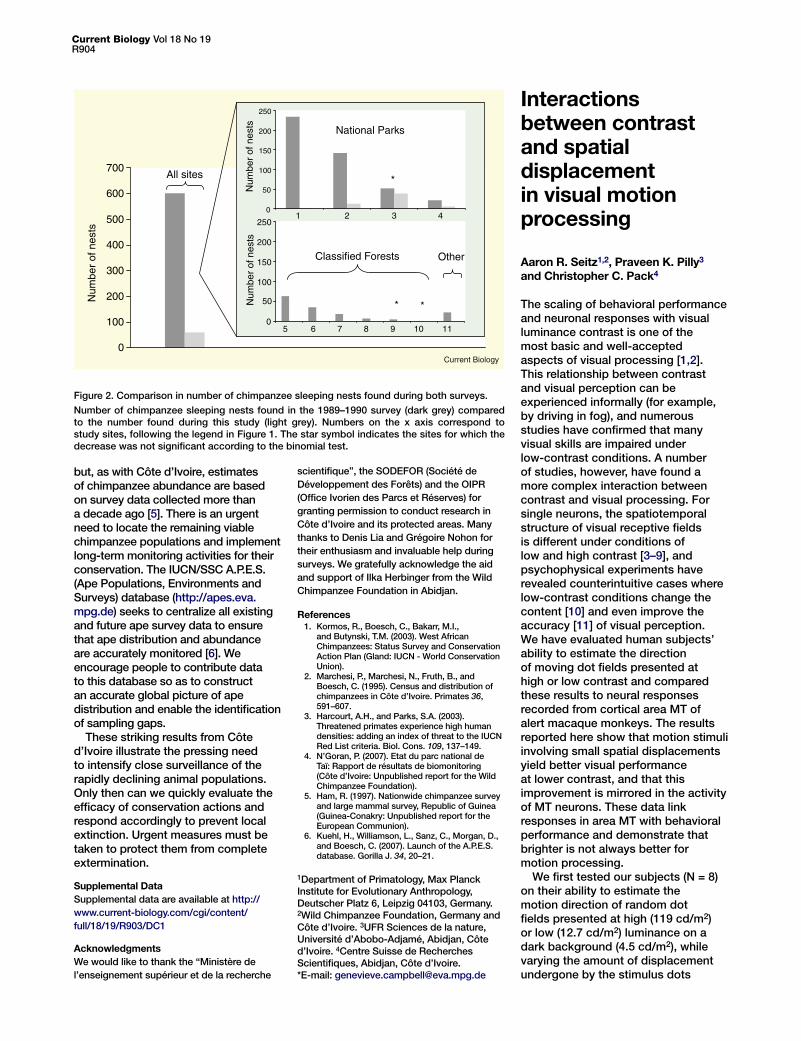
Figure 2. Comparison in number of chimpanzee sleeping nests found during both surveys.

Number of chimpanzee sleeping nests found in the 1989–1990 survey (dark grey) compared to the number found during this study (light grey). Numbers on the x axis correspond to study sites, following the legend in Figure 1. The star symbol indicates the sites for which the decrease was not significant according to the binomial test.

Interactions between contrast and spatial displacement in visual motion processing

Aaron R. Seitz1,2, Praveen K. Pilly3 and Christopher C. Pack4

The scaling of behavioral performance and neuronal responses with visual luminance contrast is one of the most basic and well-accepted aspects of visual processing [1,2]. This relationship between contrast and visual perception can be experienced informally (for example, by driving in fog), and numerous studies have confirmed that many visual skills are impaired under low-contrast conditions. A number of studies, however, have found a more complex interaction between contrast and visual processing. For single neurons, the spatiotemporal structure of visual receptive fields is different under conditions of low and high contrast [3–9], and psychophysical experiments have revealed counterintuitive cases where low-contrast conditions change the content [10] and even improve the accuracy [11] of visual perception. We have evaluated human subjects’ ability to estimate the direction of moving dot fields presented at high or low contrast and compared these results to neural responses recorded from cortical area MT of alert macaque monkeys. The results reported here show that motion stimuli involving small spatial displacements yield better visual performance at lower contrast, and that this improvement is mirrored in the activity of MT neurons. These data link responses in area MT with behavioral performance and demonstrate that brighter is not always better for motion processing.

We first tested our subjects (N = 8) on their ability to estimate the motion direction of random dot fields presented at high (119 cd/m2) or low (12.7 cd/m2) luminance on a dark background (4.5 cd/m2), while varying the amount of displacement undergone by the stimulus dots

MagazineR905

on each monitor refresh. In this task, subjects viewed a dot field for 400 ms and reported the direction by rotating the orientation of a response bar. Stimuli were shown at variable directions and temporal displacements (see Supplemental Data available on-line for detailed experimental procedures), and we manipulated motion coherence to maintain an appropriate level of task difficulty (see 100% coherence control below). We found (Figure 1A) that motion perception depended both on stimulus contrast and displacement. Surprisingly, subjects were better at determining the motion direction of stimuli with small displacements at low contrast (blue) than at high contrast (red). For larger

.04 .08 .16 .24 .32 .48 .64 20

5

10

15

20

25

30

35

40

Spatial displacement (deg)

Acc

urac

y (d

eg)

.017 .033 .067 .13 .27 .53 1.1 2.1

Nor

mal

ized

firin

g ra

te

Spatial displacement (deg)

0

0.1

0.2

0.3

0.4

0.5

0.6

0.7

0.8

0.9

1.0

A

B

Current Biology

Figure 1. Behavioral and neurophysiological results.

(A) Results of behavioral experiments. Dis-placement tuning curves for low contrast (blue; dashed) and high contrast (red; solid). Data are averaged across direction, coher-ence, and temporal displacement (data for different coherences and temporal displace-ments are given in Supplemental Figures S3, S4, S5). Accuracy is computed as the average absolute error in direction judgment subtracted from 90°; a value of 90 repre-sents perfect performance, and 0 is chance performance (distributions of errors show in Supplemental Figures S7 and S10). (B) Neu-rophysiological data from 94 MT neurons (previously described in [4]). Displacement tuning curves for low contrast (blue; dashed) and high contrast (red; solid). Error bars rep-resent standard error.

displacements this effect reversed. The interaction between contrast and displacement was highly significant (p < 0.0001; repeated-measures ANOVA) and largely independent of temporal displacement (see Table S2 and Figure S5 in the Supplemental data).

To study the potential neuronal substrate of these perceptual findings, we reanalyzed previously-published data from 94 cells recorded from area MT in two alert macaque monkeys [4]. As in the behavioral experiments, the motion stimuli were presented at low (2.2 cd/m2) or high (139.5 cd/m2) luminance on a dark background (0.025 cd/m2), and with different spatial displacements on different trials (see Supplemental data). The resulting displacement tuning functions for the neuronal population (Figure 1B) show a striking resemblance to our human behavioral data, with the interaction between displacement and contrast again being highly significant (p < 0.0001). A similar effect was observed in a smaller sample of neurons (N = 40) for which we examined the difference in responses to stimuli moving in the preferred and anti-preferred directions (see Supplemental Figure S2).

Our results demonstrate a strong similarity between the behavior of MT cells and human perception. The stimuli used in the two experiments were not identical, however, mainly because we chose to use low motion coherence in the psychophysical experiment in order to avoid ceiling effects exhibited by some observers in the 100% coherence condition. Nevertheless, to evaluate whether similar behavior would emerge with stimuli that more precisely matched those in the neurophysiology experiment, we ran 16 additional subjects with 100% coherent motion (and other matched stimulus parameters; see Supplemental Data). These results, shown in Figure 2A, replicate the original interaction between displacement and contrast (p < 0.01). As expected, many subjects were at or near ceiling performance with 100% coherent motion, which caused the profiles in Figure 1B to be blurred relative to the profiles shown in Figure 1A.

We also examined the contribution of overall stimulus luminance to psychophysical performance. This was motivated by the fact that, in the previous experiment, changing the contrast caused a slight change

in the overall stimulus luminance. To evaluate whether our results were due to changes in contrast or luminance, we tested 12 subjects with a stimulus consisting of light and dark dots on a gray background. This manipulation rendered the mean luminance constant across all conditions, but the pattern of results (Figure 2B) was largely unchanged. Again there was a highly significant interaction between contrast and displacement (p < 0.0001), suggesting an effect related to stimulus contrast, rather than luminance.

The results presented here are consistent with information-theoretic hypotheses about the influence of contrast on visual processing. To maximize information transmission, the system at high contrast suppresses redundant information [12], which, given the typical pattern of velocities on the retina during self-motion, leads to suppression of large, slow stimuli

.017 .033 .067 .13 .27 .53 1.1 2.1

Spatial displacement (deg)

.017 .033 .067 .13 .27 .53 1.1 2.1

Spatial displacement (deg)

−10

0

10

20

30

40

50

60

70

80

−10

0

10

20

30

40

50

60

70

80

Acc

urac

y (d

eg)

Acc

urac

y (d

eg)

A

B

Current Biology

Figure 2. Results of behavioral control experi-ments.

See Figure 1A for plot descriptions. (A) Exper-iment 2, displacement tuning curves for 100% coherent dot fields matching the stimulus pa-rameters of the physiological experiment (see Supplemental data for detailed experimental procedures; data for each temporal displace-ment shown in Supplemental Figure S6). (B) Experiment 3, displacement tuning curves for contrast control experiment (see Supple-mental data for detailed experimental proce-dures). Distributions of errors are shown in Supplemental Figures S8–S10).

Current Biology Vol 18 No 19R906

Primate hunting by bonobos at LuiKotale, Salonga National Park

Martin Surbeck and Gottfried Hohmann*

Chimpanzees (Pan troglodytes) and bonobos (P. paniscus) hunt and consume the meat of various mammals. While chimpanzees frequently hunt in groups for arboreal, group-living monkey species [1,2], bonobos are thought to focus on medium-sized terrestrial prey, such as forest antelopes, squirrels and other rodents, which are caught opportunistically by single individuals [3]. The absence of monkey hunting by bonobos is often used to illustrate the divergent evolution of the two Pan species [4]. Here, we present the first information on hunting of diurnal, arboreal and group living primates by wild bonobos.

Monkey hunting in chimpanzees is related to social aspects, such as bonding between males and mating effort [1,2]. The lack of monkey hunting in bonobos has been linked to a lack of male bonding and reduced levels of aggression [4,5], implying the behavior is driven not by nutritional benefits but by reproductive advantages.

We observed bonobos hunting at LuiKotale (Figure 1) in the Salonga National Park, Democratic Republic of Congo. Records on monkey hunting were obtained from members of one habituated community consisting of nine reproductive males, 12 reproductive females and 12 immatures. There were three cases of successful hunting when bonobos captured and ate monkeys and two cases in which hunting attempts did not succeed (Table 1). In all successful cases, bonobos obtained immature monkeys.

Bonobos changed their travel direction and silently approached their prey after detecting them through auditory and visual cues. When bonobos were underneath the monkey group, they stopped and several individuals took position at the bases of different trees directing their visual attention towards the

monkeys. Twice bonobos were seen to capture prey in a sudden pursuit into the trees while some individuals remained on the ground. In the third case, the actual hunt was not observed. In all cases, the monkey group had moved arboreally at a relatively low elevation (10–20 m). While the bonobos were silent during hunts, they vocalized during meat eating. Individuals who initially possessed the prey maintained control over the carcass, despite being the subject of close attention by other members of the party. As with meat-sharing in chimpanzees [1,2], individuals who possessed the carcass both actively transferred pieces of meat to other party members in response to begging gestures, and tolerated co-feeding by others on the same carcass.

It has been suggested bonobos do not hunt monkeys because aggression was selected against when ecological conditions favored female gregariousness and alliance formation [4]. An alternative view is that insufficient data from multiple bonobo populations, incomplete habituation, and effects of human interference precluded observation of monkey hunting [6]. While more data are required before conclusions can be drawn about the relationship between social traits and hunting behavior, our data raise other questions: Do the observed cases present a novel behavior? What are the environmental and social factors promoting hunting and meat eating at LuiKotale?

So far, evidence for hunting and meat eating by bonobos has largely been based on fresh fecal samples [3]. Only one sample contained the digit of a black mangabey, Cercocebus aterrhimus, but it was not entirely clear if bonobos had

Figure 1. Field sites mentioned in the text.

1: LuiKotale, 2: Lilungu, 3: Wamba.

[4]. On the other hand, at low contrast, the sole basis for distinguishing visual signal from random noise is the signal’s regularity across space and time. In this case, preserving redundancy becomes critical, and spatial pooling and temporal summation are desired.

Supplemental DataSupplemental data are available at http://www.current-biology.com/cgi/content/full/18/19/R904/DC1

AcknowledgmentsARS was supported by NSF (BCS-0549036) and NIH (R21 EY017737), PKP was supported by NIH (R01-DC02852). NSF (IIS-0205271 and SBE-0354378) and ONR (N00014-01-1-0624). CCP was supported by CIHR (MOP-79352).

References 1. Sclar, G., Maunsell, J.H., and Lennie, P. (1990).

Coding of image contrast in central visual pathways of the macaque monkey. Vision Res. 30, 1–10.

2. Shapley, R. (1990). Visual sensitivity and parallel retinocortical channels. Annu. Rev. Psychol. 41, 635–658.

3. Shapley, R.M., and Victor, J.D. (1978). The effect of contrast on the transfer properties of cat retinal ganglion cells. J. Physiol. 285, 275–298.

4. Pack, C.C., Hunter, J.N., and Born, R.T. (2005). Contrast dependence of suppressive influences in cortical area MT of alert macaque. J. Neurophysiol. 93, 1809–1815.

5. Livingstone, M.S., and Conway, B.R. (2007). Contrast affects speed tuning, space-time slant, and receptive-field organization of simple cells in macaque V1. J. Neurophysiol. 97, 849–857.

6. Peterson, M.R., Li, B., and Freeman, R.D. (2006). Direction selectivity of neurons in the striate cortex increases as stimulus contrast is decreased. J. Neurophysiol. 95, 2705–2712.

7. Polat, U., Mizobe, K., Pettet, M.W., Kasamatsu, T., and Norcia, A.M. (1998). Collinear stimuli regulate visual responses depending on cell’s contrast threshold. Nature 391, 580–584.

8. Sceniak, M.P., Ringach, D.L., Hawken, M.J., and Shapley, R. (1999). Contrast’s effect on spatial summation by macaque V1 neurons. Nat. Neurosci. 2, 733–739.

9. Krekelberg, B., van Wezel, R.J., and Albright, T.D. (2006). Adaptation in macaque MT reduces perceived speed and improves speed discrimination. J. Neurophysiol. 95, 255–270.

10. Stone, L.S., and Thompson, P. (1992). Human speed perception is contrast dependent. Vision Res. 32, 1535–1549.

11. Tadin, D., Lappin, J.S., Gilroy, L.A., and Blake, R. (2003). Perceptual consequences of centre-surround antagonism in visual motion processing. Nature 424, 312–315.

12. van Hateren, J.H. (1992). Real and optimal neural images in early vision. Nature 360, 68–70.

1Department of Psychology, University of California, Riverside, Riverside, California 92521, USA. 2Department of Psychology, Boston University, Boston, Massachusetts 02215, USA. 3Department of Cognitive and Neural Systems, Boston University, Boston, Massachusetts 02215, USA. 4Montreal Neurological Institute, McGill University School of Medicine, Montreal, Quebec, Canada H3A 2B4. E-mail: aseitz@ucr.edu, christopher.pack@mcgill.ca

Supplemental Data: Interactions between contrast and spatial displacement in visual motion

processing

Aaron R Seitz, Praveen K. Pilly, and Christopher C. Pack

Supplemental Experimental Procedures

Behavioral Experiments

Experiment 1

Subjects. 8 naïve human subjects (1 male, 7 female: 18-33 years), with normal or corrected-to-

normal vision, participated in the experiment for two, one-hour, sessions conducted on different

days. The experiments were conducted in accordance with the IRB approved by the Committee

on Human Research of the Boston University and the Declaration of Helsinki.

Apparatus. Subjects sat on a height-adjustable chair, with the head stabilized in a chin rest, at a

viewing distance of 60 cm from the center of a Dell P991 (Trinitron) CRT monitor (36 cm in

width). The monitor was set to a resolution of 1024 x 768 pixels, and a refresh rate of 120 Hz.

Experiments were conducted in a dimly lit room to minimize the effects of dark adaptation.

Stimuli were generated and presented using Psychtoolbox Version 2 [S1, S2] with MATLAB

5.2.1 (MathWorks, Inc.) on a Mac G4 machine running OS9.

Stimuli. Motion stimuli consisted of random dot fields [S3]. White dots of high contrast (119

cd/m2) or low contrast (12.7 cd/m2) were shown on a dark background (4.5 cd/m2). Each dot was

a 3 x 3 pixel square, and subtended a visual angle of ~0.1o on the eyes. Dots were displayed

within an 8o diameter invisible circular aperture located at the center of the screen. Dot density

was fixed at 16.7 dots deg-2/s. From one frame to the next, a probabilistic fraction of the dots,

determined by the coherence level, was randomly selected to move in the signal direction with a

particular spatial displacement, while the remaining dots were relocated to random locations

within the aperture. For example, in a 15% coherent motion display, 15% of the dots in a

successive frame moved in the same direction and speed (signal dots) while the remaining 85%

were replaced randomly (noise dots). On each trial the dot field was presented at one of eight

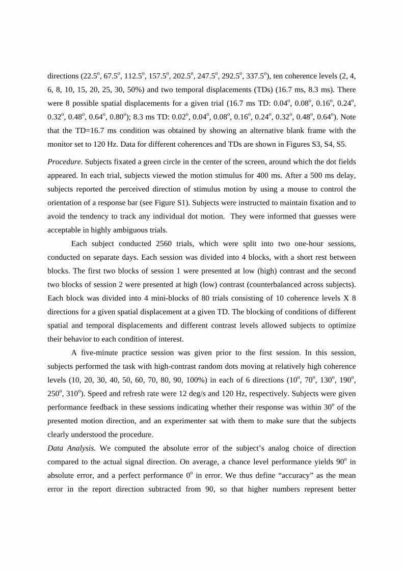
directions (22.5o, 67.5o, 112.5o, 157.5o, 202.5o, 247.5o, 292.5o, 337.5o), ten coherence levels (2, 4,

6, 8, 10, 15, 20, 25, 30, 50%) and two temporal displacements (TDs) (16.7 ms, 8.3 ms). There

were 8 possible spatial displacements for a given trial (16.7 ms TD: 0.04o, 0.08o, 0.16o, 0.24o,

0.32o, 0.48o, 0.64o, 0.80o); 8.3 ms TD: 0.02o, 0.04o, 0.08o, 0.16o, 0.24o, 0.32o, 0.48o, 0.64o). Note

that the TD=16.7 ms condition was obtained by showing an alternative blank frame with the

monitor set to 120 Hz. Data for different coherences and TDs are shown in Figures S3, S4, S5.

Procedure. Subjects fixated a green circle in the center of the screen, around which the dot fields

appeared. In each trial, subjects viewed the motion stimulus for 400 ms. After a 500 ms delay,

subjects reported the perceived direction of stimulus motion by using a mouse to control the

orientation of a response bar (see Figure S1). Subjects were instructed to maintain fixation and to

avoid the tendency to track any individual dot motion. They were informed that guesses were

acceptable in highly ambiguous trials.

Each subject conducted 2560 trials, which were split into two one-hour sessions,

conducted on separate days. Each session was divided into 4 blocks, with a short rest between

blocks. The first two blocks of session 1 were presented at low (high) contrast and the second

two blocks of session 2 were presented at high (low) contrast (counterbalanced across subjects).

Each block was divided into 4 mini-blocks of 80 trials consisting of 10 coherence levels X 8

directions for a given spatial displacement at a given TD. The blocking of conditions of different

spatial and temporal displacements and different contrast levels allowed subjects to optimize

their behavior to each condition of interest.

A five-minute practice session was given prior to the first session. In this session,

subjects performed the task with high-contrast random dots moving at relatively high coherence

levels (10, 20, 30, 40, 50, 60, 70, 80, 90, 100%) in each of 6 directions (10o, 70o, 130o, 190o,

250o, 310o). Speed and refresh rate were 12 deg/s and 120 Hz, respectively. Subjects were given

performance feedback in these sessions indicating whether their response was within 30o of the

presented motion direction, and an experimenter sat with them to make sure that the subjects

clearly understood the procedure.

Data Analysis. We computed the absolute error of the subject’s analog choice of direction

compared to the actual signal direction. On average, a chance level performance yields 90o in

absolute error, and a perfect performance 0o in error. We thus define “accuracy” as the mean

error in the report direction subtracted from 90, so that higher numbers represent better

performance. Statistical analysis consisted of a 4-way repeated measure ANOVA with Spatial

Displacement X Contrast X Coherence X Temporal Displacement as factors. The use of a

repeated measures ANOVA treats subjects as an additional factor and is appropriate to show

validity of the effect across subjects.

Control Experiments

Subjects. 16 additional, naïve human subjects (8 male, 8 female: 18-35 years), with normal or

corrected-to-normal vision, participated in the control experiment for a single one-hour session.

All subjects participated in the first control experiment (with parameters matching the

physiological experiment), while a subset (n=12; 6 male, 6 female: 18-35 years) also participated

in the second control experiment (evaluating the effects of contrast).

Experiment 2: Control for neurophysiological parameters. In this experiment we matched

stimulus parameters as closely as possible to those used in the neurophysiological experiment.

Methods were similar to Experiment 1 except for a few differences.

We used 100% coherent dot motion. In a pilot experiment we determined that with a

viewing duration of 100 ms subjects could achieve reasonable displacement tuning functions

even at 100% coherence, although some subjects still showed ceiling effects in some conditions.

A ViewSonic P225f CRT monitor, with a horizontal width of 40 cm, was used. This

monitor had a desirable range of producible luminance levels (0-122 cd/m2) in dim illumination,

especially on the lower side (0-2.2 cd/m2). The use of this monitor was necessary to match the

luminance values used in the neurophysiological experiment. All subjects also participated in a

practice session in the beginning of the session.

We also matched our stimuli to the average eccentricity, aperture size and dot density

used in the physiological experiment. On each trial, the 8o diameter stimulus aperture was

centered at a random location at 8o eccentricity. A random direction of motion was also chosen

on each trial to minimize the effect of response biases. Average dot density was fixed at 30 dots

deg-2/s (0.5 dots deg-2 at 60 Hz).

Stimuli consisted of white dots (high: 122 cd/m2 or low: 2.2 cd/m2) moving on a black

background (~0 cd/m2). 3 TDs (8.3, 16.7, 33.3 ms) and 8 SDs (0.017, 0.033, 0.067, 0.13, 0.27,

0.53, 1.07, 2.13o) were used with 24 trials per condition. The total of 1152 trials was divided into

4 blocks with a short rest period between blocks. The first two blocks presented high (low)

contrast dots, and the other two blocks low (high) contrast dots (counterbalanced across

subjects). In either contrast condition, TD and SD were randomly interleaved. The TD=33.3 ms

condition was obtained by showing 3 blank frames in alternation with the monitor set to 120 Hz.

Data for different TDs shown in Figure S6.

Experiment 3: control for contrast. In this experiment, methods were similar to those described

above except for the following differences. Stimuli consisted of an equal number of white (high:

120 cd/m2 or low: 80 cd/m2) and black (high: 0 cd/m2 or low: 40 cd/m2) dots moving on a grey

background (60 cd/m2) at 100% motion coherence. Mean luminance was thus identical between

the two contrast conditions. Only 1 TD (16.7 ms) was used, and the monitor refresh rate was set

to 60 Hz. We found that uncertainty about the location of the stimulus drastically affected

stimulus detection at this high mean luminance (60 cd/m2), so we introduced a positional cue

(0.5o diameter red point) at the centre of the stimulus 400 ms before motion onset. The cue

disappeared when motion began.

Data Analysis. In the control for physiological parameters, statistical analysis consisted of a 3-

way repeated measure ANOVA with Spatial Displacement X Contrast X Temporal

Displacement as factors. In the control for contrast, statistical analysis consisted of a 2-way

repeated measure ANOVA with Spatial Displacement X Contrast as factors.

Neurophysiological Experiment

Extracellular recordings. The neurophysiological data came from a previously published study

[S4] and were reanalyzed for comparison with the human behavioral data. Recordings were

obtained from single units in two alert monkeys, as described previously [S5]. Each animal

underwent a MRI scan to locate MT within the coordinates of a plastic grid inserted in the

recording cylinder. The same grid, along with a guide tube, was used to guide insertion of the

microelectrode. MT was identified based on depth, prevalence of direction-selective neurons,

receptive field size, and visual topography. Neuronal signals were recorded extracellularly using

tungsten microelectrodes (FHC) with standard amplification and filtering (BAK Electronics),

while the monkeys fixated a small spot. Fixation was monitored with an eye coil [S6] and

required to be within 1o of the spot for the monkeys to obtain a liquid reward. Single units were

isolated using a dual time and amplitude window discriminator (BAK). All procedures were

approved by the Harvard Medical Area Standing Committee on Animals.

Stimuli. Visual stimuli were presented on a computer monitor subtending 40o by 30o at a viewing

distance of 57 cm. The refresh rate was 60 Hz. The stimuli consisted of 100% coherent dot fields

presented on a dim background (0.025 cd/m2), and were viewed binocularly. The dot fields were

presented in square apertures, with no blurring along the edges. 8 SDs (0.017, 0.033, 0.067, 0.13,

0.27, 0.53, 1.07, 2.13o) and 1 TD (16.7 ms) were employed. Dot luminance was 139.5 cd/m2 in

the high contrast condition and 2.2 cd/m2 in the low contrast condition. Each dot subtended

~0.1o, and the average dot density was 0.5 dots/deg2 (or equivalently 30 dots deg-2/s). For each

neuron, we first collected a direction-tuning curve at high contrast, adjusting the size and speed

manually to obtain robust responses from the neuron. We then measured displacement tuning

curves at the preferred direction with stimulus size chosen to approximate the size of the hand-

mapped classical receptive field. For some cells we also collected data for stimuli moving at

different spatial displacements in the null direction, which was defined to be 180o away from the

preferred direction. Mean eccentricity of the MT population was 8o (SD 4.3o). Each stimulus was

presented 5-10 times in block-wise random order for 1 s.

Data analysis. Data for each experiment were averaged over the full 1000 ms stimulus

presentation. Figure 1b shows the average of the normalized response of each cell for each

contrast level. Statistical analysis consisted of a 2-way repeated measure ANOVA with

Displacement X Contrast as factors.

Supplemental References

S1. Brainard, D.H. (1997). The Psychophysics Toolbox. Spat Vis 10, 433-436. S2. Pelli, D.G. (1997). The VideoToolbox software for visual psychophysics: transforming

numbers into movies. Spat Vis 10, 437-442. S3. Britten, K.H., Shadlen, M.N., Newsome, W.T., and Movshon, J.A. (1992). The analysis

of visual motion: a comparison of neuronal and psychophysical performance. J Neurosci 12, 4745-4765.

S4. Pack, C.C., Hunter, J.N., and Born, R.T. (2005). Contrast dependence of suppressive influences in cortical area MT of alert macaque. J Neurophysiol 93, 1809-1815.

S5. Born, R.T., Groh, J.M., Zhao, R., and Lukasewycz, S.J. (2000). Segregation of object and background motion in visual area MT: effects of microstimulation on eye movements. Neuron 26, 725-734.

S6. Robinson, D. (1963). A method of measuring eye movement using a scleral search coil in a magnetic field. IEEE Transactions on Biomedical Engineering 10, 137-145.

Supplemental Tables and Figures

Exp. 1 Exp. 2 Exp. 3 Neurophysiology Mean luminance (low) – cd/m2 4.52 0.01 60 0.04

Mean luminance (high) – cd/m2 4.82 0.76 60 0.72

RMS contrast (low) – cd/m2 0.44 0.17 1.58 0.15

RMS contrast (high) – cd/m2 6.08 9.62 4.75 9.83

Table S1: Contrast and Luminance. For spatially non-periodic stimuli, contrast is better defined by the standard deviation of individual pixel luminance values than by the Michelson formula. Note that in Experiments 1 and 3 the mean luminance between the two contrast conditions is not very different: 6.65% and 0% relative difference, respectively, and hence only stimulus contrast was manipulated.

Comparison (p-value) Coherence .0001 Spatial Displacement (SD) .0001 Temporal Displacement (TD) 0.012 Contrast 0.55 Contrast * SD .0001 Contrast * SD * TD 0.43 Contrast * SD * Coherence .0001

Table S2: Statistical Results of Experiment 1. Main effects for Coherence and Spatial Displacement were expected. Notably, the lack of a main effect for contrast indicates that overall performance is similar between the high- and low-contrast conditions. The lack of an interaction of Temporal Displacement with Contrast and Spatial Displacement indicates that the interaction of interest did not differ across the two Temporal Displacements used, indicating that Spatial Displacement (rather than actual Speed) is fundamental in determining our effects. However, the interaction of Coherence with Contrast and Spatial Displacement is largely influenced by the floor effects at low contrast (see Figures S2, S3).

Comparison (p-value) Spatial Displacement (SD) 0.0001 Temporal Displacement (TD) 0.0001 Contrast 0.16 Contrast * SD .008 Contrast * SD * TD 0.06

Table S3: Statistical Results of Experiment 2. Main effects for Spatial Displacement were expected. However the lack of a main effect for contrast indicates that overall performance is similar between the high and low contrast conditions. The lack of an interaction of Temporal Displacement with Contrast and Spatial Displacement indicates that the interaction of interest did not differ across the three Temporal Displacements used.

Figure S1 – Task Schematic. In each trial, subjects viewed a random dot stimulus for 400 ms; after a delay of 500 ms they selected their response by rotating a bar to correspond with the perceived motion direction.

Figure S2 – Neurophysiological data from 40 MT neurons for which responses were recorded for cells’ preferred and null directions. Rates for each SD show difference between response to preferred and null direction for low contrast (blue; dashed) and high contrast (red; solid). Note that the SDs differ slightly from those used in the main experiment (Figure 1b), but the overall pattern of results is the same. Error bars represent standard error.

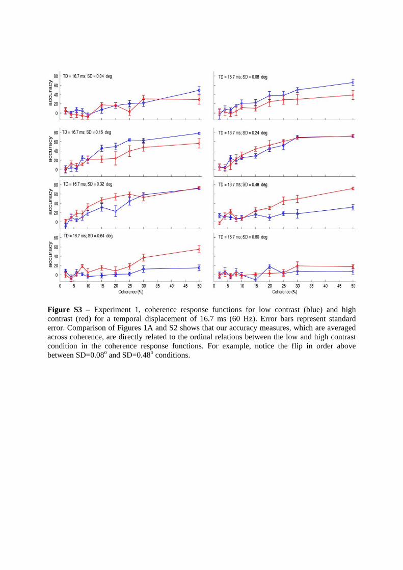
Figure S3 – Experiment 1, coherence response functions for low contrast (blue) and high contrast (red) for a temporal displacement of 16.7 ms (60 Hz). Error bars represent standard error. Comparison of Figures 1A and S2 shows that our accuracy measures, which are averaged across coherence, are directly related to the ordinal relations between the low and high contrast condition in the coherence response functions. For example, notice the flip in order above between SD=0.08o and SD=0.48o conditions.

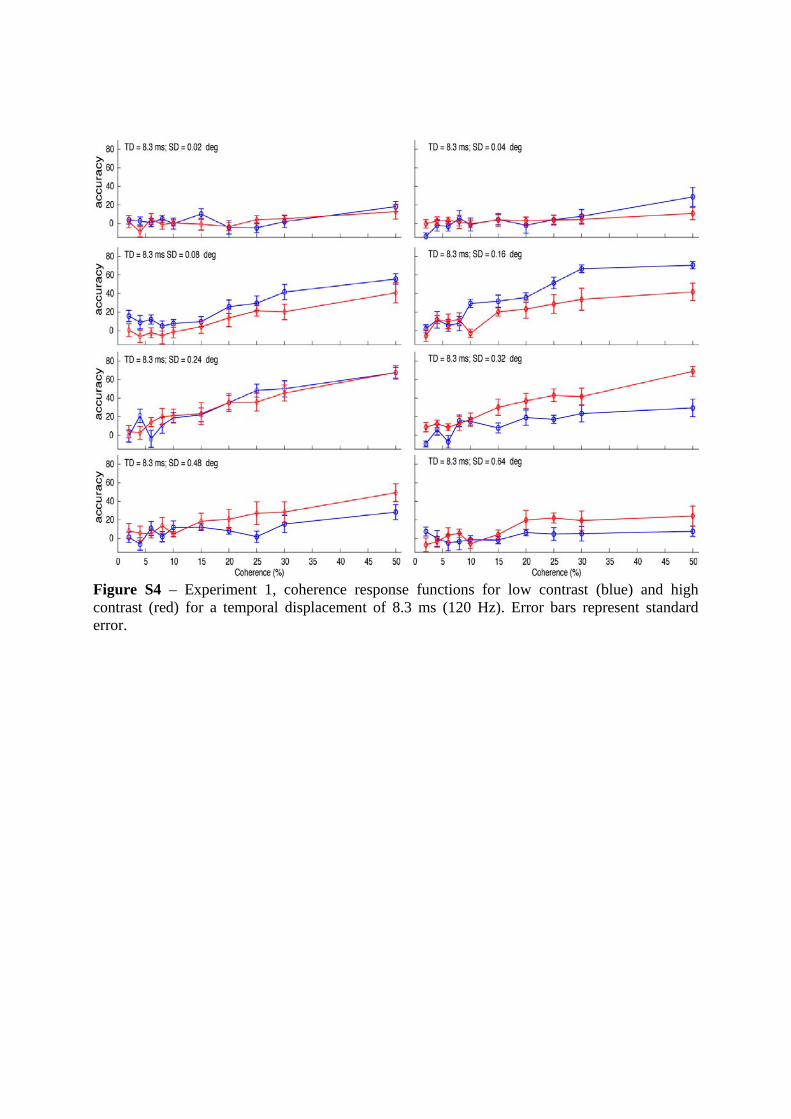
Figure S4 – Experiment 1, coherence response functions for low contrast (blue) and high contrast (red) for a temporal displacement of 8.3 ms (120 Hz). Error bars represent standard error.

Figure S5 – Experiment 1, SD response functions for TD=16.7 ms (top) and TD= 8.33 ms (bottom) for low contrast (blue; dashed) and high contrast (red; solid). Error bars represent standard error.

Figure S6 – Experiment 2, SD response functions for TD=33.3 ms (top), TD=16.7 ms (middle) and TD= 8.33 ms (bottom) for low contrast (blue; dashed) and high contrast (red; solid). Error bars represent standard error.

Figure S7 – Distribution of errors for each SD of Experiment 1 for low contrast (blue; dashed) and high contrast (red; solid) conditions. Perfect performance would be represented as a line segment from the center of the figure pointing to the right. Chance performance would be represented as a circle. Each point represents the count of errors within a 30° bin centered at the point.

Figure S8 – Distribution of errors for each SD of Experiment 2 for low contrast (blue; dashed) and high contrast (red; solid) conditions. Perfect performance would be represented as a line segment from the center of the figure pointing to the right. Chance performance would be represented as a circle. Each point represents the count of errors within a 30° bin centered at the point.

Figure S9 – Distribution of errors for each SD of Experiment 3 for low contrast (blue; dashed) and high contrast (red; solid) conditions. Perfect performance would be represented as a line segment from the center of the figure pointing to the right. Chance performance would be represented as a circle. Each point represents the count of errors within a 30° bin centered at the point.

Figure S10 – Distribution of responses within 60° of the correct direction (thick line) or opposite direction (thin line) for low contrast (blue; dashed) and high contrast (red; solid) conditions of Experiment 1 (top), Experiment 2 (middle) and Experiment 3 (bottom) Error bars represent standard error.