LBNL-39795UC-1600

INTERACTIONS BETWEEN LIGHTING AND SPACECONDITIONING ENERGY USE IN U.S. COMMERCIAL

BUILDINGS

Osman Sezgen and Jonathan G. Koomey

Energy Analysis DepartmentEnvironmental Energy Technologies Division

Ernest Orlando Lawrence Berkeley National LaboratoryUniversity of California

Berkeley, CA 94720, USA

http://enduse.lbl.gov/projects/CommData.html

April 1998

This work was supported by the Assistant Secretary for Energy Efficiency and Renewable Energy, Office of BuildingTechnologies, State and Community Programs of the U.S. Department of Energy under Contract No. DE-AC03-76SF00098.

i

ABSTRACT

Reductions in lighting energy have secondary effects on cooling and heating energy consumption.In general, lighting energy reductions increase heating and decrease cooling requirements of abuilding. The net change in a building's annual energy requirements, however, is difficult toquantify and depends on the building characteristics, operating conditions, and climate.

This paper characterizes the effects of lighting/HVAC interactions on the annual heating/coolingrequirements of prototypical U.S. commercial buildings through computer simulations using theDOE-2.1E building energy analysis program. Twelve building types of two vintages and fiveclimates are chosen to represent the U.S. commercial building stock. For each combination ofbuilding type, vintage, and climate, a prototypical building is simulated with varying lightingpower densities, and the resultant changes in heating and cooling loads are recorded. These loadsare used together with market information on the saturation of the different HVAC equipment in thecommercial buildings to determine the changes in energy use and expenditures for heating andcooling.

Results are presented by building type for the US as a whole. Therefore, the data presented in thispaper can be utilized to assess the secondary effects of lighting-related federal policies withwidespread impacts, like minimum efficiency standards. Generally, in warm climates theinteractions will induce monetary savings and in cold climates the interactions will induce monetarypenalties. For the commercial building stock in the U.S., a reduction in lighting energy that is welldistributed geographically will induce neither significant savings nor significant penalties fromassociated changes in HVAC primary energy and energy expenditures.

ii

ACKNOWLEDGMENTS

We would like to thank Dave Belzer of Pacific Northwest National Laboratory, Steven Nadel ofAmerican Council for an Energy Efficient Economy, and Joe Huang, Isaac Turiel, Leslie Shownand Steven Konopacki of EOL Berkeley National Laboratory for reviewing this report and theirmany helpful comments.

This work was supported by the Assistant Secretary for Energy Efficiency and Renewable Energy,Office of Building Technologies, State and Community Programs of the U.S. Department ofEnergy under Contract No. DE-AC03-76SF00098.

iii

TABLE OF CONTENTS

ABSTRACT . . . . . . . . . . . . . . . . . . . . . . . . . . . . . . . . . . . . . . . . . . . . . . . . . . . . . . . . . . . . . . . . . . . . I

INTRODUCTION . . . . . . . . . . . . . . . . . . . . . . . . . . . . . . . . . . . . . . . . . . . . . . . . . . . . . . . . . . . . . . 1

METHODOLOGY . . . . . . . . . . . . . . . . . . . . . . . . . . . . . . . . . . . . . . . . . . . . . . . . . . . . . . . . . . . . . . 3

Designing and simulating prototype commercial buildings .. . . . . . . . . . . . . . . . . . . . . . . . .3

Development of HVAC saturations and efficiencies.. . . . . . . . . . . . . . . . . . . . . . . . . . . . . . . . .6

Integration of data and determination of energy and monetary effects of interactions.. . . . . . . . . . . . . . . . . . . . . . . . . . . . . . . . . . . . . . . . . . . . . . . . . . . . . . . . . . . . . . . . . . . . . . . . . . . . . . . . . . . . . . . . . . . . .8

RESULTS . . . . . . . . . . . . . . . . . . . . . . . . . . . . . . . . . . . . . . . . . . . . . . . . . . . . . . . . . . . . . . . . . . . . . . 8

DISCUSSION . . . . . . . . . . . . . . . . . . . . . . . . . . . . . . . . . . . . . . . . . . . . . . . . . . . . . . . . . . . . . . . . . . 1 6

LIMITATIONS OF THIS ANALYSIS AND FUTURE WORK . . . . . . . . . . . . . 1 6

CONCLUSIONS . . . . . . . . . . . . . . . . . . . . . . . . . . . . . . . . . . . . . . . . . . . . . . . . . . . . . . . . . . . . . . . 1 7

REFERENCES . . . . . . . . . . . . . . . . . . . . . . . . . . . . . . . . . . . . . . . . . . . . . . . . . . . . . . . . . . . . . . . . . 1 8

APPENDIX A: PROTOTYPE SIMULATIONS . . . . . . . . . . . . . . . . . . . . . . . . . . . . . . 1 9

APPENDIX B: HVAC SYSTEM AND PLANT SATURATIONS . . . . . . . . . . 2 4

APPENDIX C: EFFICIENCY DATA FOR HVAC PLANT OPTIONS . . . . . 2 7

iv

LIST OF TABLES

Table 1a: Changes in building loads, energy use, and energy expenditures caused by onekWh decline in lighting load, a one kWh decline in lighting energy use, or a one dollardecline in lighting energy expenditures in existing commercial buildings.. . . . . . . . . . . . . . . . . .4

Table 1b: Changes in building loads, energy use, and energy expenditures caused by onekWh decline in lighting load, a one kWh decline in lighting energy use, or a one dollardecline in lighting energy expenditures in new commercial buildings.. . . . . . . . . . . . . . . . . . . . . .5

Table A.1: The 36 Commercial Building Prototypes .. . . . . . . . . . . . . . . . . . . . . . . . . . . . . . . . . . . . . . . .20

Table A.2. Cities Representing the CBECS Climate Categories .. . . . . . . . . . . . . . . . . . . . . . . . . . . .21

Table A.3: System Load Multipliers (U.S. Average).. . . . . . . . . . . . . . . . . . . . . . . . . . . . . . . . . . . . . . . .23

Table B.1: Saturations of Combinations of Heating/Cooling Equipment and SystemOptions (Stock Buildings) .. . . . . . . . . . . . . . . . . . . . . . . . . . . . . . . . . . . . . . . . . . . . . . . . . . . . . . . . . . . . . . . . . . . . . . .25

Table B.2: Saturations of Combinations of Heating/Cooling Equipment and SystemOptions (New Buildings) .. . . . . . . . . . . . . . . . . . . . . . . . . . . . . . . . . . . . . . . . . . . . . . . . . . . . . . . . . . . . . . . . . . . . . . . .26

Table C.1: Seasonal Heating and Cooling-Plant Efficiency Data.. . . . . . . . . . . . . . . . . . . . . . . . . . .28

v

LIST OF FIGURES

Figure 1: Structure of The Analysis.. . . . . . . . . . . . . . . . . . . . . . . . . . . . . . . . . . . . . . . . . . . . . . . . . . . . . . . . . . . .2

Figure 2: Saturation of heating/cooling combinations in the commercial sector--Allbuilding types (fraction of total commercial sector floor area).. . . . . . . . . . . . . . . . . . . . . . . . . . . . . . .7

Figure 3a: Change in Heating and Cooling Loads Caused by a 1 kWh Decline in LightingLoads in Existing Commercial Buildings .. . . . . . . . . . . . . . . . . . . . . . . . . . . . . . . . . . . . . . . . . . . . . . . . . . . . .10

Figure 3b: Change in Heating and Cooling Loads Caused by a 1 kWh Decline in LightingLoads in New Commercial Buildings .. . . . . . . . . . . . . . . . . . . . . . . . . . . . . . . . . . . . . . . . . . . . . . . . . . . . . . . . .11

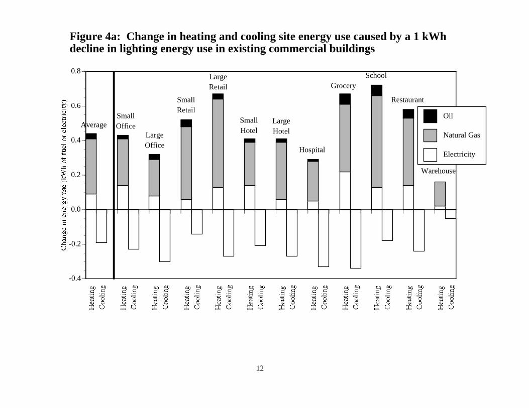
Figure 4a: Change in Heating and Cooling Site Energy Use Caused by a 1 kWh Decline inLighting Energy Use in Existing Commercial Buildings.. . . . . . . . . . . . . . . . . . . . . . . . . . . . . . . . . . . . .12

Figure 4b: Change in Heating and Cooling Site Energy Use Caused by a 1 kWh Decline inLighting Energy Use in New Commercial Buildings.. . . . . . . . . . . . . . . . . . . . . . . . . . . . . . . . . . . . . . . . .13

Figure 5a: Change in Heating and Cooling Energy Expenditures Caused by a $1 Decline inLighting Energy Expenditures in Existing Commercial Buildings .. . . . . . . . . . . . . . . . . . . . . . . . . .14

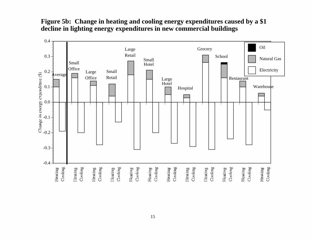
Figure 5b: Change in Heating and Cooling Energy Expenditures Caused by a $1 Decline inLighting Energy Use in New Commercial Buildings.. . . . . . . . . . . . . . . . . . . . . . . . . . . . . . . . . . . . . . . . .15

1

INTRODUCTION

There has been ongoing controversy over the size of changes in heating and cooling energy useassociated with reductions of lighting energy use in commercial buildings. Many analysts haveassumed that cooling savings totaling one third of the savings in lighting energy can be achievedbecause of interactions between lighting and HVAC (Heating, Ventilation, and Air Conditioning).However, these analysts have traditionally ignored the heating penalties. This report calculates themagnitude of the cooling benefits and heating penalties using a state-of-the-art data set for thecommercial sector.

In a previous study, Sezgen and Huang (1994a) presented the effects of lighting/HVACinteractions on annual and peak HVAC requirements in commercial buildings. In that study, tencommercial building types of two vintages are simulated using the DOE-2.1E building energyanalysis program, and the effect of reductions of lighting energy use on annual and peak HVACloads are presented in look-up tables. These tables can be used to estimate the changes in annualheating and cooling loads in a given building type and region, but the study does not carry throughthe calculation to heating and cooling energy.

A somewhat similar approach is used by Rundquist et al. (1993) and Johnson (1996) to estimatethe effects of lighting reduction on HVAC energy. This approach does not use prototypes for eachbuilding type. Instead, the perimeter area of the building is determined, and loads are calculated asa function of surface area to volume ratio. Again, lookup tables are presented to show how theHVAC loads will change in different climates. Finally, simple calculations using approximateefficiencies of HVAC system and plant are used to determine indirect energy effects.

Franconi and Rubinstein (1992) assess lighting/HVAC interactions in large office buildings fortwo HVAC system types in two climates. Treado and Bean (1992) evaluate the interactions ofbuilding lighting and HVAC systems, and the effects on cooling load and lighting performanceusing a full-scale test facility for selected equipment configurations. While not comprehensive inscope, these works are exemplary in their detailed treatment of these interactions for the specificcases considered.

Our analysis builds on the Sezgen and Huang (1994a) work, and characterizes the impacts oflighting/HVAC interactions on the annual heating/cooling energy of prototypical U.S. commercialbuildings. We characterize HVAC system and plant types and associated efficiencies, and convertload results to energy results for the U.S. as a whole. The results are applicable to any policy thataffects lighting or plug loads and has direct energy savings impacts that are geographically well-distributed around the country.

We first describe the methodology and present the results. We discuss the importance of thoseresults, and assess limitations of and possible improvements to the analysis.

2

Figure 1: Structure of The Analysis

DOE-2

Effects of the type ofDistribution System onLoads and Distribution System Electricity Use

Lighting/HVAC Coincidence Factors

SPREADSHEET MODEL

Results:• Changes in heating and cooling energy and expenditures by building type due to an incremental change in lighting energy

CBECS

Building Prototypes:•12 Building Types• South and North• Stock and New• 9 Distribution System Configurations (eg, Variable Air Volume with Reheat and Economizer, Hydronic)

HVAC System and PlantSaturations including Economizers and Controls

Efficiency of HVACPlant Components:•15 Plant Components (eg. Gas Boiler, Air- Source Heat Pump, Electric Chiller)• Stock and New

Engineering ExpertiseClimate Data:• 5 Representative Locations

Other Data

3

METHODOLOGY

Our analysis has three main parts: designing and simulating prototype commercial buildings indifferent regions, characterizing the efficiency of space conditioning equipment, and integrating theefficiency data and the results of those simulations to estimate overall average effects for the U.S. Figure 1 summarizes the overall methodology. Changes in heating and cooling energyconsumption are a function of the interaction between the lighting and HVAC loads, equipmentsaturations, plant efficiencies, and distribution system efficiencies.

Designing and simulating prototype commercial buildings

Because the building and operating characteristics of commercial buildings are very different forthe different building types (e.g. office buildings, warehouses, hospitals), it is inaccurate torepresent such buildings with a single commercial sector prototype. In Sezgen et al. (1995), usingthe results of the CBECS (US DOE/EIA, 1992), we developed prototypes for the differentbuilding types. This set of prototypes gives an accurate national picture of building characteristicsin the U.S., properly accounting for equipment saturations, distribution-system characteristics,equipment efficiencies, and shell characteristics.

The climate also plays an important role in the way lighting and HVAC end uses interact. For thisreason we differentiated our prototypes by region. We simulated the energy behavior of ourprototypes under five different climate assumptions. Results of such simulations yielded: (1)building loads and lighting/HVAC coincidence factors, and (2) effects of HVAC distributionsystem on the building loads.

Building Loads and Coincidence Factors

In our analysis, the building load is defined as the amount of heating or cooling the system mustsupply to a building to meet the temperature set-points. Because we wanted to include the loadfrom ventilation with the building load, we developed a user-defined DOE-2 function to modify theload calculation so that it included the outdoor air load during the hours that the system fan wasscheduled to be on. The ventilation requirement for the modeled buildings is 15 ft3 of fresh air perperson per minute. The model determines the total flow rate based on the building's occupantdensity, floor area, and ventilation requirement.

One of the outputs of the DOE-2 simulations is the HVAC load. By varying the lighting levels inthe prototypes in parametric simulation runs, we characterized the interaction between the lightingloads and the HVAC loads. Coincidence factors are used to characterize the interaction betweenend uses, as described in Sezgen and Huang (1994a). Cooling coincidence factors for lightingrepresent the fraction of annual energy input for lighting that ends up as an internal heat gain duringthe cooling period. Similarly, heating coincidence factors give the amount of annual lighting energythat ends up as internal gain during heating periods. The coincidence factors are presented inTables 1a and 1b.

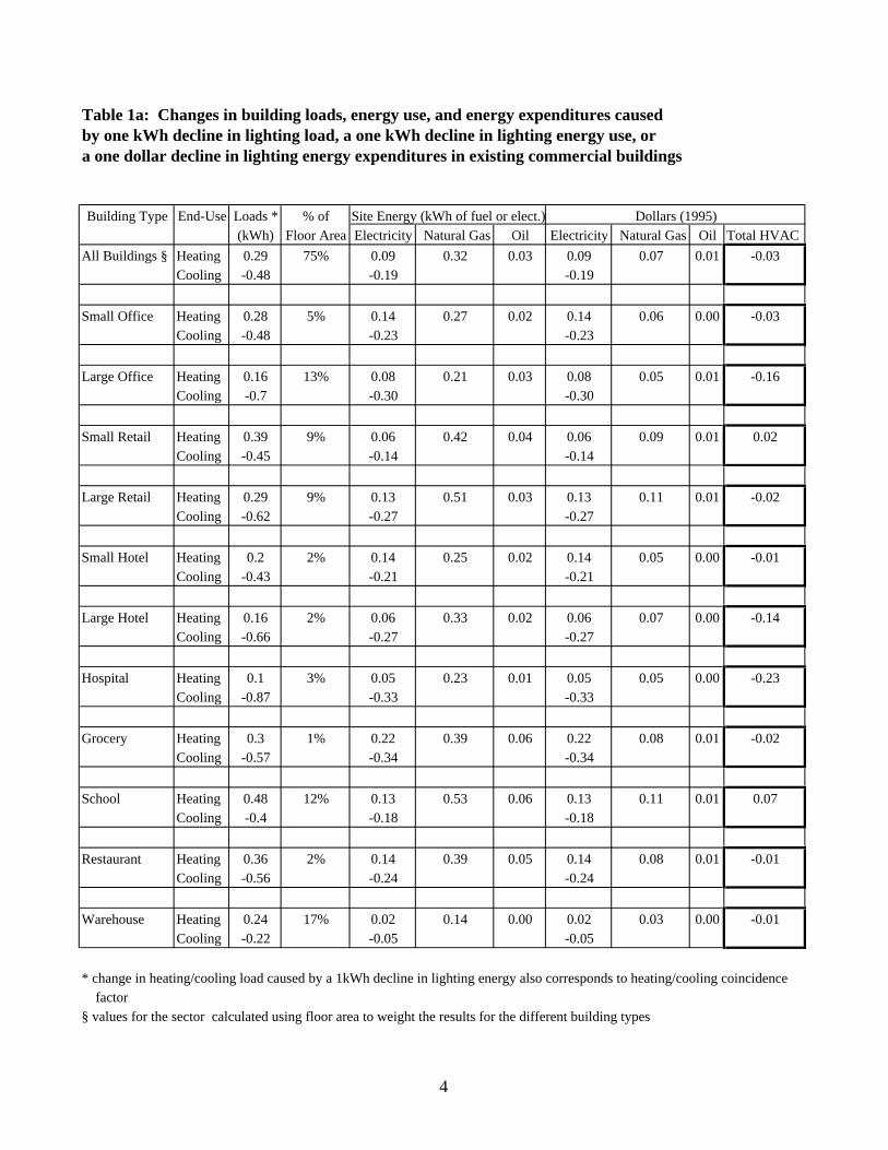
Table 1a: Changes in building loads, energy use, and energy expenditures caused by one kWh decline in lighting load, a one kWh decline in lighting energy use, or a one dollar decline in lighting energy expenditures in existing commercial buildings

Building Type End-Use Loads * % of Site Energy (kWh of fuel or elect.) Dollars (1995)(kWh) Floor Area Electricity Natural Gas Oil Electricity Natural Gas Oil Total HVAC

All Buildings § Heating 0.29 75% 0.09 0.32 0.03 0.09 0.07 0.01 -0.03Cooling -0.48 -0.19 -0.19

Small Office Heating 0.28 5% 0.14 0.27 0.02 0.14 0.06 0.00 -0.03Cooling -0.48 -0.23 -0.23

Large Office Heating 0.16 13% 0.08 0.21 0.03 0.08 0.05 0.01 -0.16Cooling -0.7 -0.30 -0.30

Small Retail Heating 0.39 9% 0.06 0.42 0.04 0.06 0.09 0.01 0.02Cooling -0.45 -0.14 -0.14

Large Retail Heating 0.29 9% 0.13 0.51 0.03 0.13 0.11 0.01 -0.02Cooling -0.62 -0.27 -0.27

Small Hotel Heating 0.2 2% 0.14 0.25 0.02 0.14 0.05 0.00 -0.01Cooling -0.43 -0.21 -0.21

Large Hotel Heating 0.16 2% 0.06 0.33 0.02 0.06 0.07 0.00 -0.14Cooling -0.66 -0.27 -0.27

Hospital Heating 0.1 3% 0.05 0.23 0.01 0.05 0.05 0.00 -0.23Cooling -0.87 -0.33 -0.33

Grocery Heating 0.3 1% 0.22 0.39 0.06 0.22 0.08 0.01 -0.02Cooling -0.57 -0.34 -0.34

School Heating 0.48 12% 0.13 0.53 0.06 0.13 0.11 0.01 0.07Cooling -0.4 -0.18 -0.18

Restaurant Heating 0.36 2% 0.14 0.39 0.05 0.14 0.08 0.01 -0.01Cooling -0.56 -0.24 -0.24

Warehouse Heating 0.24 17% 0.02 0.14 0.00 0.02 0.03 0.00 -0.01Cooling -0.22 -0.05 -0.05

* change in heating/cooling load caused by a 1kWh decline in lighting energy also corresponds to heating/cooling coincidence factor§ values for the sector calculated using floor area to weight the results for the different building types

4

Table 1b: Changes in building loads, energy use, and energy expenditures caused by one kWh decline in lighting load, a one kWh decline in lighting energy use, or a one dollar decline in lighting energy expenditures in new commercial buildings

Building Type End-Use Loads* % of Site Energy (kWh of fuel or elect.) Dollars (1995)kWh Floor Area Electricity Natural Gas Oil Electricity Natural Gas Oil Total HVAC

All Buildings § Heating 0.27 76% 0.10 0.25 0.01 0.10 0.05 0.00 -0.03Cooling -0.50 -0.19 -0.19

Small Office Heating 0.29 5% 0.16 0.16 0.01 0.16 0.03 0.00 0.00Cooling -0.46 -0.20 -0.20

Large Office Heating 0.15 16% 0.11 0.15 0.01 0.11 0.03 0.00 -0.13Cooling -0.7 -0.28 -0.28

Small Retail Heating 0.36 12% 0.04 0.37 0.00 0.04 0.08 0.00 -0.01Cooling -0.46 -0.13 -0.13

Large Retail Heating 0.23 11% 0.18 0.41 0.00 0.18 0.09 0.00 -0.04Cooling -0.72 -0.31 -0.31

Small Hotel Heating 0.19 0% 0.15 0.27 0.00 0.15 0.06 0.00 0.00Cooling -0.45 -0.20 -0.20

Large Hotel Heating 0.12 0% 0.05 0.24 0.00 0.05 0.05 0.00 -0.16Cooling -0.69 -0.27 -0.27

Hospital Heating 0.06 0% 0.03 0.10 0.00 0.03 0.02 0.00 -0.24Cooling -0.91 -0.29 -0.29

Grocery Heating 0.16 1% 0.26 0.23 0.00 0.26 0.05 0.00 0.00Cooling -0.73 -0.31 -0.31

School Heating 0.44 11% 0.16 0.42 0.04 0.16 0.09 0.01 0.02Cooling -0.42 -0.24 -0.24

Restaurant Heating 0.24 2% 0.10 0.18 0.01 0.10 0.04 0.00 -0.13Cooling -0.69 -0.28 -0.28

Warehouse Heating 0.25 18% 0.04 0.10 0.00 0.04 0.02 0.00 0.01Cooling -0.23 -0.05 -0.05

* change in heating/cooling load caused by a 1kWh decline in lighting energy also corresponds to heating/cooling coincidence

factor

§ values for the sector calculated using floor area to weight the results for the different building types

5

6

HVAC Distribution System Load Factors and Electrical Energy Use

The system load is the amount of heating and cooling the HVAC plant has to provide to thedistribution system for the building load to be met. The system load factor is a multiplier used withthe base-case building load to translate the building load to the system load; the system factor variesdepending on the type of distribution system and its control strategy. In addition to affecting theheating and cooling loads, the HVAC system uses electrical energy to drive fans and pumps.

System load factors were calculated as the ratio of the system load to the building load (both ofwhich are DOE-2 outputs). System electricity use is calculated as the sum of the pump and fanelectricity use. For air conditioners, packaged unitary systems, and heat-pump loops, the systemefficiency and the system electricity use are included as part of the plant efficiency. System loadfactors and electrical energy use for different building types are presented in Appendix A (sectionA3). We did not utilize the data on system electricity use in this report because the difference ofelectricity used by the pumps and the fans between the scenarios with different lighting levels is notsignificant.

Economizers tend to decrease the system loads under suitable conditions. The data on which werelied characterize this effect comparing the outputs of parametric runs with and withouteconomizers. However, the market penetration of economizers is not significant with the exceptionof large office buildings where this penetration was around 8% in 1989. Therefore in this study weignored the effect of economizers.

Development of HVAC saturations and efficiencies

One of the key issues in estimating the potential energy effects of changes in lighting loads is theprevalence (saturation) of different combinations of heating and cooling equipment. Directestimations of the saturation of HVAC equipment combinations are not possible using only the1989 CBECS. However, we combined the CBECS data with engineering judgment regarding thecompatibility of combinations of heating/cooling equipment and distribution systems to estimatesaturations by building type. Saturations of heating/cooling equipment combinations are shown inFigure 2 for both stock and new buildings (more detailed data, and data by building type, arecontained in Tables B.1 and B.2 in Appendix B). We ignored the less important equipmentcombinations within each building type to create a rough characterization of these saturations.

Plant and distribution system efficiencies are another key input to the analysis. We rely on annualintegrated part load efficiencies that reflect operational differences over a typical year (Table C.1 inAppendix C). These efficiencies are then multiplied by the annual loads to estimate annual energyuse. Integrated part load efficiencies are generally less than efficiency measured under full loadconditions.

0.00

0.02

0.04

0.06

0.08

0.10

0.12

0.14

0.16

Stock

New

Figure 2: Saturation of heating/cooling combinations in the commercialsector--All building types (fraction of total commercial sector floor area)

Source: CBECS 1989 and engineering judgement,as described in A. O. Sezgen, E. M. Franconi, J. G. Koomey, S. E. Greenberg,and A. Afzal. 1995. Technology data characterizing space conditioning incommercial buildings: Application to end-use forecasting with COMMEND4.0. Lawrence Berkeley Laboratory. LBL-37065. December.

Ducted systems Unitary systems Fan coil systemsHydronicsystems

7

8

Integration of data and determination of energy and monetary effects o finteractions

The market shares for the different equipment types by building type are combined with (1) heatingand cooling coincidence factors by building type; (2) plant efficiencies; and (3) distribution systemlosses to calculate the change in HVAC energy use due to a unit reduction in lighting energy. Aunit reduction in lighting changes the heating and cooling loads by amounts determined by thecoincidence factors. These incremental changes in heating and cooling loads need to be satisfied bythe HVAC system. These changes in building loads are first modified using the system load factorsto account for distribution system losses and then multiplied by plant efficiencies to determine thechanges in fuel use. Finally, the change in fuel use is multiplied by fuel prices1 to determine themonetary impact of interactions.

RESULTS

A reduction in lighting energy causes a reduction in cooling load and an increase in heating load.Figures 3a and 3b presents the changes in heating/cooling loads due to a one unit (kWh) changein lighting energy (these can also be read from Tables 1a and 1b above). These changes correspondto the coincidence factors mentioned above. The annual energy coincidence factors for heating andcooling in general correlate to the duration of the heating and cooling seasons of the buildings.However, there is noticeably less coincidence for heating as compared to cooling, even when thelengths of the seasons are considered, because the lights are almost always on when cooling isrequired during the day, but frequently off when heating is required during the night.

For larger building types, the sums of the heating and cooling coincidence factors are larger,indicating that any changes in their lighting power density ultimately manifest themselves inmodifying the buildings' heating or cooling loads. For the smaller or less energy-intensivebuildings such as lodging or warehouse buildings, the sum of coincidence factors is lower. Thecoincidence factor for cooling is very high in hospitals because internal gains are high and thesebuildings are being cooled most of the time. In schools and colleges, the heating coincidencefactors are larger than the other building types because the percentage of activity during the heatingseason is larger in these building types. Generally, cooling coincidence factors are larger thanheating coincidence factors. The building types in which heating coincidence factors are larger areschools and warehouses: again, in educational buildings the activity is more during the heatingseason, and in warehouses cooling is utilized usually only in the offices which constitute a smallarea of this building type.

How these changes in cooling and heating loads affect the energy use and energy expendituresdepends on the saturations of the different kinds of HVAC equipment. In terms of site energy, asseen in Figures 4a and 4b (also summarized in Tables 1a and 1b), the penalty due to heating ishigher than the gains due to cooling. Although the increase in heating load is generally less than thedecrease in cooling loads in absolute terms, more site energy is needed to satisfy one unit ofheating load compared to one unit of cooling loads. Reductions in lighting energy increase HVACsite energy use in all building types (the increase in heating site energy is larger than the reductionin cooling energy) except in hospitals.

1 Fuel prices are taken from US DOE/EIA (1996). The prices are for 1995 in 1995 dollars.

9

The picture changes somewhat when we examine expenditures (which also parallel the situation atthe primary energy level). As seen from Figures 5a and 5b (also summarized in Tables 1a and1b), the changes in heating and cooling expenditures are comparable, with benefits outweighingpenalties by a small margin (3-4%). Benefits significantly dominate penalties in large offices, largehotels, hospitals, and new restaurants. Penalties significantly dominate benefits in schools.Electricity is generally three times more expensive than other fuels, and cooling equipment ispredominantly driven by electricity. When considering expenditures, the higher price of electricityoffsets the lower site energy use for cooling, and brings cooling benefits close to heating penalties.

-1.0

-0.8

-0.6

-0.4

-0.2

0.0

0.2

0.4

0.6

0.8

1.0

Figure 3a. Change in heating and cooling loads caused by a 1 kWh decline inlighting loads in existing commercial buildings

AverageSmallOffice Large

Office

SmallRetail Large

Retail GroceryWarehouse

School

LargeHotel

Hospital

SmallHotel

Restaurant

10

-1.0

-0.8

-0.6

-0.4

-0.2

0.0

0.2

0.4

0.6

0.8

1.0

Figure 3b. Change in heating and cooling loads caused by a 1 kWh decline inlighting loads in new commercial buildings

AverageSmallOffice Large

Office

SmallRetail Large

RetailGrocery

Warehouse

School

LargeHotel

Hospital

SmallHotel

Restaurant

11

-0.4

-0.2

0.0

0.2

0.4

0.6

0.8

Electricity

Natural Gas

Oil

Figure 4a: Change in heating and cooling site energy use caused by a 1 kWhdecline in lighting energy use in existing commercial buildings

AverageSmallOffice

LargeOffice

SmallRetail

LargeRetail

SmallHotel

LargeHotel

Hospital

GrocerySchool

Restaurant

Warehouse

12

-0.4

-0.2

0.0

0.2

0.4

0.6

0.8

Electricity

Natural Gas

Oil

Figure 4b: Change in heating and cooling site energy use caused by a 1 kWhdecline in lighting energy use in new commercial buildings

Average SmallOffice Large

OfficeRestaurant

SmallRetail

Grocery

Warehouse

School

LargeHotel

Hospital

LargeRetail

SmallHotel

13

-0.4

-0.3

-0.2

-0.1

0.0

0.1

0.2

0.3

0.4

Electricity

Natural Gas

Oil

Figure 5a: Change in heating and cooling energy expenditures caused by a $1decline in lighting energy expenditures in existing commercial buildings

Average

SmallOffice

LargeOffice

Restaurant

LargeRetail

Grocery

Warehouse

School

LargeHotel

Hospital

SmallHotelSmall

Retail

14

-0.4

-0.3

-0.2

-0.1

0.0

0.1

0.2

0.3

0.4

Electricity

Natural Gas

Oil

Figure 5b: Change in heating and cooling energy expenditures caused by a $1decline in lighting energy expenditures in new commercial buildings

Average

SmallOffice

LargeOffice Restaurant

SmallRetail

Grocery

Warehouse

School

Hospital

SmallHotel

LargeRetail

LargeHotel

15

16

DISCUSSION

The building types covered in this report constitute about 75 percent of the commercial buildingarea in the US. For this section of the commercial floor stock, the net reduction in HVAC bills dueto a reduction in lighting is about 3.4 percent of the change in lighting bill. This report presents theresults in terms of site energy and energy expenditures, and not in terms of source energy.However, for the above mentioned section of the commercial building area, the change in HVACsource energy due to lighting/HVAC interactions is approximately zero.

One may wonder how the lighting/HVAC interactions in the other 25 percent of the commercialfloorstock will change this picture. Vacant buildings, garages, buildings for religious worship,buildings related to public order and safety, and public assembly buildings (including theaters,conference halls) make up this 25 percent of the commercial floorstock for which we did notdevelop prototypes. About 4 percent of the commercial floor area is vacant and therefore usesminimal HVAC energy. Garages are about 2.5 percent of the floor area and again use practicallyno HVAC energy and therefore there is no need to analyze the secondary effects of lighting energyreduction on HVAC energy use. Buildings for religious worship constitute about 5 percent of thearea and such buildings can be loosely compared to warehouses (some offices but mostly openspace with some heating). Therefore we can assume that there will not be significant savings due tolighting/HVAC interactions in these buildings. Buildings related to public order and safetyconstitute about 2.5 percent of the commercial floor area and again these building types are verysimilar to warehouses. About 7 percent of the commercial floorstock is assembly buildings. Insuch buildings there might be net savings in HVAC energy bills due to lighting/HVACinteractions. Buildings which are not included in any of the above mentioned building typesconstitute about 4 percent of the commercial area and it is not possible to characterize them. It isclear that the only building type that will affect our results and conclusions is related publicassembly buildings. If we assume that the situation in public assembly buildings is as favorable asthat in large office buildings (net gain in HVAC expenditure equal to an amount which is 16percent of the gain in lighting bill), the overall secondary dollar savings of 3.4 percent for allbuilding types will increase to 4.6 percent.

The main application of this analysis is to policies that promote efficient lighting equipment (or anyother efficient equipment that reduces internal gains in commercial buildings) in all commercialbuildings across the U.S. One example of such a policy would be the minimum efficiencystandard on ballasts passed in 1988 as an amendment to the National Appliance EnergyConservation Act of 1987. This standard eliminated the manufacture and sale of inefficientmagnetic ballasts throughout the U.S. starting in 1990 (Koomey et al., 1996). The results of ouranalysis could be used to assess the overall secondary effects on HVAC energy use from thisefficiency standard.

These results should not be used to draw conclusions about the importance of HVAC interactionsin particular buildings or building types in particular regions. For example, it would beinappropriate and incorrect to use our results to assess HVAC interactions in a particular largeoffice building in San Francisco or New York. Our results for large office buildings represent anaverage across five climate zones and all HVAC system types found in large offices throughout theU.S., and would be misleading for any assessment of interactions in a particular building.

LIMITATIONS OF THIS ANALYSIS AND FUTURE WORK

The data set generated for this report has much more detail than used in this report. For thepurposes of this report, we averaged prototype simulation results for the different climate regions.In other words we suppressed information on regional characteristics. The methodology of thisreport can be applied to the more detailed data set to generate useful information to building

17

designers and for local analysis purposes. Such an effort would calculate and report the HVACinteraction results by building type and by region of the U.S.

Another area of future work is to update the analysis to reflect more recent survey data oncommercial building characteristics (e.g., CBECS 1995).

CONCLUSIONS

This study examines the effects of lighting/HVAC interactions on the HVAC energy consumptionof the U.S. building stock as a whole, as a result of uniform reductions in lighting energy. Thefindings apply to the analysis of lighting policies like standards at the federal level. In summary,for the commercial building stock in the U.S., a reduction in lighting energy that is well-distributedgeographically and across building types will induce neither significant savings nor significantpenalties in HVAC primary energy and small benefits in HVAC energy expenditures.

When lighting/HVAC interactions are examined regionally, the picture is different. Generally, inwarm climates the interactions will induce monetary savings and in cold climates the interactionswill induce monetary penalties. Region-specific and building-specific analyses would be requiredto deduce precise conclusions for particular regions and buildings.

18

REFERENCES

EPAct. 1992. Energy Policy Act of 1992. US House of Representatives. Conference Report 102-1018 to accompany H.R. 776. US Government Printing Office, Washington, DC. October 5th.

Franconi, Ellen, and Francis Rubinstein. 1992. "Considering Lighting System Performance andHVAC Interactions in Lighting Retrofit Analysis". Presented at 1992 IEEE Industry ApplicationsSociety Annual Meeting in Houston, Texas. Published in the IAS Conference Record. October 4-9, 1992., vol. II., pp. 1858-1867.

Johnson, K. 1996. "Energy Policies in Action." LD+A, September.

Koomey, Jonathan, Alan H. Sanstad, and Leslie J. Shown. 1996. "Energy-Efficient Lighting:Market Data, Market Imperfections, and Policy Success." Contemporary Economic Policy. vol.XIV, no. 3. p. 98.

Rundquist, R., K.F. Johnson, and D.J. Aumann. 1993. "Calculating Lighting and HVACInteractions," ASHRAE Journal, Nov.

Sezgen, O., and Y.J. Huang. 1994a. Lighting/HVAC Interactions and Their Effects on Annualand Peak HVAC Requirements in Commercial Buildings. LBL-36524. Lawrence BerkeleyNational Laboratory, Berkeley, CA. (Also published in the proceedings of 1994 ACEEE SummerStudy.)

Sezgen, A.O., Y.J. Huang, B.A. Atkinson, J.H. Eto, and J.G. Koomey. 1994b. TechnologyData Characterizing Lighting in Commercial Buildings : Application to End-Use Forecasting WithCOMMEND 4.0. LBL- 34243, Lawrence Berkeley National Laboratory, Berkeley, CA.

Sezgen, Osman, Ellen M. Franconi, Jonathan G. Koomey, Steve E. Greenberg, Asim Afzal, andLeslie Shown. 1995. Technology Data Characterizing Space Conditioning in CommercialBuildings: Application to End-Use Forecasting with COMMEND 4.0. LBL-37065. LawrenceBerkeley National Laboratory, Berkeley, CA. December.

U.S. Department of Energy/Energy Information Administration (US DOE/EIA), 1992.Commercial Building Energy Consumption Survey 1989: Characteristics of Commercial Buildings1989. DOE/EIA-0246(89), U.S. Department of Energy, Washington, D.C.

U.S. Department of Energy/Energy Information Administration (US DOE/EIA), 1996. AnnualEnergy Outlook 1997. DOE/EIA-0383(97), U.S. Department of Energy, Washington, D.C.

Treado, S.J. and J.W. Bean. 1992. The Interactions of Lighting, Heating and Cooling Systems inBuildings. NISTIR-4701. U.S. Department of Commerce, Technology Administration, NationalInstitute of Standards and Technology, Gaithersburg, MD. March.

19

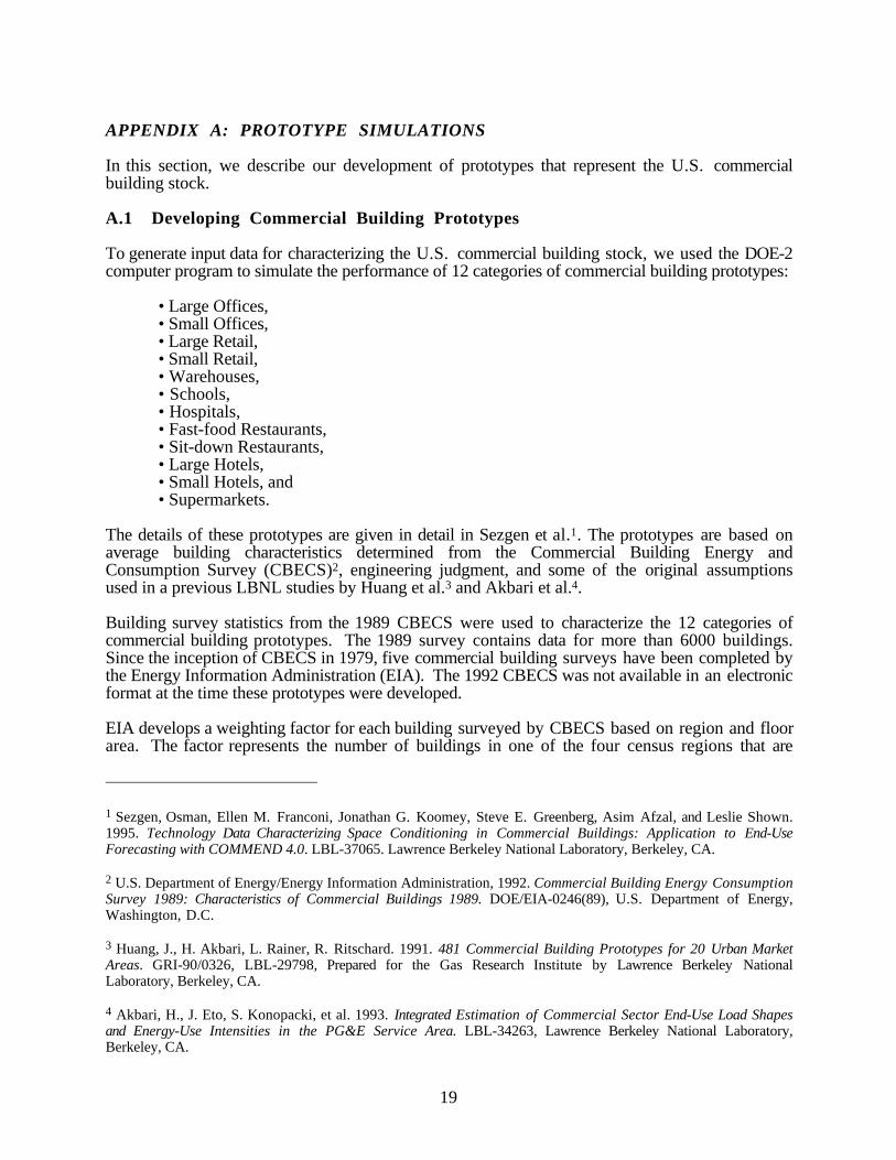
APPENDIX A: PROTOTYPE SIMULATIONS

In this section, we describe our development of prototypes that represent the U.S. commercialbuilding stock.

A.1 Developing Commercial Building Prototypes

To generate input data for characterizing the U.S. commercial building stock, we used the DOE-2computer program to simulate the performance of 12 categories of commercial building prototypes:

• Large Offices,• Small Offices,• Large Retail,• Small Retail,• Warehouses,• Schools,• Hospitals,• Fast-food Restaurants,• Sit-down Restaurants,• Large Hotels,• Small Hotels, and• Supermarkets.

The details of these prototypes are given in detail in Sezgen et al.1. The prototypes are based onaverage building characteristics determined from the Commercial Building Energy andConsumption Survey (CBECS)2, engineering judgment, and some of the original assumptionsused in a previous LBNL studies by Huang et al.3 and Akbari et al.4.

Building survey statistics from the 1989 CBECS were used to characterize the 12 categories ofcommercial building prototypes. The 1989 survey contains data for more than 6000 buildings.Since the inception of CBECS in 1979, five commercial building surveys have been completed bythe Energy Information Administration (EIA). The 1992 CBECS was not available in an electronicformat at the time these prototypes were developed.

EIA develops a weighting factor for each building surveyed by CBECS based on region and floorarea. The factor represents the number of buildings in one of the four census regions that are

1 Sezgen, Osman, Ellen M. Franconi, Jonathan G. Koomey, Steve E. Greenberg, Asim Afzal, and Leslie Shown.1995. Technology Data Characterizing Space Conditioning in Commercial Buildings: Application to End-UseForecasting with COMMEND 4.0. LBL-37065. Lawrence Berkeley National Laboratory, Berkeley, CA.

2 U.S. Department of Energy/Energy Information Administration, 1992. Commercial Building Energy ConsumptionSurvey 1989: Characteristics of Commercial Buildings 1989. DOE/EIA-0246(89), U.S. Department of Energy,Washington, D.C.

3 Huang, J., H. Akbari, L. Rainer, R. Ritschard. 1991. 481 Commercial Building Prototypes for 20 Urban MarketAreas. GRI-90/0326, LBL-29798, Prepared for the Gas Research Institute by Lawrence Berkeley NationalLaboratory, Berkeley, CA.

4 Akbari, H., J. Eto, S. Konopacki, et al. 1993. Integrated Estimation of Commercial Sector End-Use Load Shapesand Energy-Use Intensities in the PG&E Service Area. LBL-34263, Lawrence Berkeley National Laboratory,Berkeley, CA.

20

similar to the surveyed building in terms of floor area. The weighting factor and the floor area ofeach surveyed building are used to extrapolate total floor area by building type. We also used thisCBECS weighting factor to determine building characteristics related to floor area such as shell andoccupancy. We assume that buildings of the same type and floor area, if they are located in thesame region, have the same construction, equipment, and operating characteristics. Although thisis not necessarily precisely correct, using the weighting factor to characterize many buildings basedon a sample of buildings is a reasonable first-order approximation.

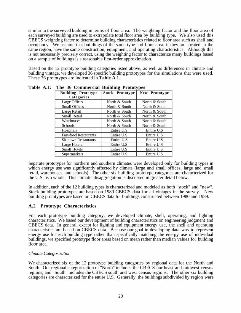
Based on the 12 prototype building categories listed above, as well as differences in climate andbuilding vintage, we developed 36 specific building prototypes for the simulations that were used.These 36 prototypes are indicated in Table A.1.

Table A.1: The 36 Commercial Building PrototypesBuilding Prototype

CategoriesStock Prototype New Prototype

Large Offices North & South North & SouthSmall Offices North & South North & SouthLarge Retail North & South North & SouthSmall Retail North & South North & SouthWarehouses North & South North & SouthSchools North & South North & SouthHospitals Entire U.S Entire U.SFast-food Restaurants Entire U.S Entire U.SSit-down Restaurants Entire U.S Entire U.SLarge Hotels Entire U.S Entire U.SSmall Hotels Entire U.S Entire U.SSupermarkets Entire U.S Entire U.S

Separate prototypes for northern and southern climates were developed only for building types inwhich energy use was significantly affected by climate (large and small offices, large and smallretail, warehouses, and schools). The other six building prototype categories are characterized forthe U.S. as a whole. This climatic disaggregation is discussed in greater detail below.

In addition, each of the 12 building types is characterized and modeled as both "stock" and "new".Stock building prototypes are based on 1989 CBECS data for all vintages in the survey. Newbuilding prototypes are based on CBECS data for buildings constructed between 1980 and 1989.

A.2 Prototype Characteristics

For each prototype building category, we developed climate, shell, operating, and lightingcharacteristics. We based our development of building characteristics on engineering judgment andCBECS data. In general, except for lighting and equipment energy use, the shell and operatingcharacteristics are based on CBECS data. Because our goal in developing data was to representenergy use for each building type rather than specifically matching the energy use of individualbuildings, we specified prototype floor areas based on mean rather than median values for buildingfloor area.

Climate Categorization

We characterized six of the 12 prototype building categories by regional data for the North andSouth. Our regional categorization of "North" includes the CBECS northeast and midwest censusregions; and "South" includes the CBECS south and west census regions. The other six buildingcategories are characterized for the entire U.S. Generally, the buildings subdivided by region were

21

better represented in the CBECS data base because they make up a larger percentage of thecommercial building floor area.

Table A.2 presents five CBECS degree-day categories and the five cities that we chose torepresent these climate categories: Minneapolis, Chicago, Washington D.C., Pasadena, andCharleston. Table 3.2 also presents the cooling degree days (CDD) and heating degree days(HDD) for each of the five cities. Minneapolis and Pasadena were selected because they are largepopulation centers within their climate classification. Chicago and Charleston were selectedbecause they represent the population-weighted average climate for the northern and southernU.S., respectively. Washington, D.C. was selected because it is the population-weighted, nationalaverage climate5. The CDD and HDD for these five cities represent those for the entire zone.

Table A.2. Cities Representing the CBECS Climate Categories

CBECS Climate Classification Location CDD* HDD*

Zone 1: CDD<2000; HDD>7000 Minneapolis 750 8070

Zone 2: CDD<2000; 5500<HDD<7000 Chicago 998 6194

Zone 3: CDD<2000; 4000<HDD<5500 Washington, D.C. 1425 4236

Zone 4: CDD<2000; HDD<4000 Pasadena 1053 1670

Zone 5: CDD>2000; HDD<4000 Charleston 2047 2193* At 65˚ F

For the six building types that were modeled using regional data, the floorstock in Zones 1 and 2was modeled using the North prototypes and the appropriate climates (Minneapolis and Chicago,respectively). The floorstock in Zones 4 and 5 was modeled using the South prototypes and thecorresponding climate data (Pasadena and Charleston, respectively). The floorstock in Zone 3,represented by Washington, D.C. climate data, is divided into two parts. One part of Zone 3'sfloorstock is modeled using the North prototypes and the other part is modeled using the Southprototypes. For the remaining six building types that were not modeled using regional prototypes,the same prototype was simulated in all five climates.

Shell Characteristics

To specify shell characteristics for the prototypes, we used floor area weighted averagesdetermined from CBECS "present" or "not present" percentages and nominal R-values which wespecified. For wall insulation, we used a nominal value of R-7. For roof insulation, the nominalvalue was R-14. For windows, the nominal value for single glazing was R-1.1; for double glazing(storm windows present) the value was R-2.0. To determine the prototype shading coefficient(SC), we averaged nominal SC values for tinted and non-tinted single- and double-panedwindows. We assumed that if 40% of the windows were reported to be tinted, 40% of both thesingle-paned and double-paned windows were tinted. To calculate the SC for each prototype, weset the SC of single-paned non-tinted office windows to 0.9, single-paned tinted windows to 0.75,

5 Andersson, B., W. Carroll, and R.M. Marlo. 1986. Aggregation of U.S. Population Centers Using ClimateParameters Related to Building Energy Use. Journal of Climate and Applied Meteorology, Vol. 25, Issue 5, pp. 596-614.

22

double-paned non-tinted windows to 0.77, double-paned tinted windows to 0.65, and found theweighted average.

Operating and Lighting Characteristics

CBECS provides limited information regarding energy end uses. For lighting, CBECS specifiesthe percentage of floor area lit by different categories of lighting equipment, but the extent to whichthe systems overlap and the amount of energy they use is not provided. In addition, details onoffice equipment are not requested by the survey. The energy use of lighting and equipment that isspecified in the prototypes is based on values established in previous prototype studies andmeasured end-use studies3 4 6 7. When reconciling inconsistent lighting power density values fromdifferent studies, we used the CBECS equipment combination data to choose the more appropriatevalue.

System Prototypes

Efficiencies of the different HVAC systems are also developed through prototype simulations.Each prototype building described above is modeled with the following nine HVAC systems:

• Hydronic• Constant-Volume Reheat• Constant-Volume Reheat with Economizer• Multizone• Multizone with Economizer• Variable-Air-Volume with Reheat• Variable-Air-Volume with Reheat and Economizer• Fan-Coil• Heat-Pump Loop

A.3 System Multipliers

The system load multipliers used in this study are presented in Table A.3. These multipliers areresults of the prototype simulations. Building loads or changes in building loads are multiplied bythese factors before they are multiplied by plant efficiency factors to determine the fuel use. Thesemultipliers account for duct losses and also heat added to the system by the distribution systemfans and pumps that need to be removed by the HVAC plant equipment.

6 NEOS Corporation. 1993. Technology Energy Savings: Summary of Building Prototype Descriptions and DetailedMeasures Tables. Prepared for the California Conservation Inventory Group by NEOS Corporation, Sacramento,CA.

7 Sezgen, A.O., Y.J. Huang, B.A. Atkinson, J.H. Eto, and J.G. Koomey. 1994. Technology Data CharacterizingLighting in Commercial Buildings : Application to End-Use Forecasting With COMMEND 4.0. LBL- 34243,Lawrence Berkeley National Laboratory, Berkeley, CA.

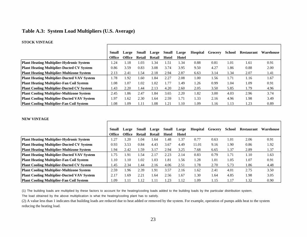
Table A.3: System Load Multipliers (U.S. Average)

STOCK VINTAGE

Small Large Small Large Small Large Hospital Grocery School Restaurant WarehouseOffice Office Retail Retail Hotel Hotel

Plant Heating Multiplier-Hydronic System 1.24 1.18 1.03 1.34 1.51 1.34 0.88 0.81 1.01 1.61 0.91Plant Heating Multiplier-Ducted CV System 0.86 3.59 0.83 3.08 3.74 3.95 9.50 4.27 1.86 0.88 2.00Plant Heating Multiplier-Multizone System 2.13 2.41 1.54 2.18 2.94 2.87 6.63 3.14 1.34 2.07 1.41Plant Heating Multiplier-Ducted VAV System 1.78 1.92 1.60 1.84 2.27 2.08 1.00 1.56 1.71 1.16 1.67Plant Heating Multiplier-Fan Coil System 1.08 1.07 1.02 1.02 1.77 1.49 1.26 0.99 1.04 1.09 0.91Plant Cooling Multiplier-Ducted CV System 1.43 2.20 1.44 2.13 4.20 2.60 2.05 3.50 5.85 1.79 4.96Plant Cooling Multiplier-Multizone System 2.45 1.86 2.47 1.84 3.65 2.20 1.82 3.00 4.03 2.96 3.74Plant Cooling Multiplier-Ducted VAV System 1.97 1.62 2.30 1.64 2.59 1.71 1.33 2.16 4.96 1.98 3.49Plant Cooling Multiplier-Fan Coil System 1.08 1.09 1.11 1.08 1.21 1.10 1.09 1.16 1.13 1.23 0.89

NEW VINTAGE

Small Large Small Large Small Large Hospital Grocery School Restaurant WarehouseOffice Office Retail Retail Hotel Hotel

Plant Heating Multiplier-Hydronic System 1.27 1.20 1.04 1.64 1.48 1.37 0.77 0.63 1.01 2.06 0.91Plant Heating Multiplier-Ducted CV System 0.93 3.53 0.84 4.43 3.67 4.49 11.01 9.16 1.90 0.86 1.92Plant Heating Multiplier-Multizone System 1.94 2.42 1.59 3.17 2.94 3.25 7.68 6.65 1.37 2.89 1.37Plant Heating Multiplier-Ducted VAV System 1.75 1.91 1.54 2.17 2.23 2.14 0.83 0.79 1.71 1.10 1.63Plant Heating Multiplier-Fan Coil System 1.10 1.10 1.02 1.03 1.81 1.56 1.28 1.01 1.05 1.07 0.91Plant Cooling Multiplier-Ducted CV System 1.45 2.34 1.44 2.16 4.06 2.51 1.78 2.70 5.73 1.86 4.48Plant Cooling Multiplier-Multizone System 2.59 1.96 2.39 1.91 3.57 2.16 1.62 2.41 4.01 2.75 3.50Plant Cooling Multiplier-Ducted VAV System 2.17 1.69 2.21 1.64 2.56 1.67 1.30 1.64 4.85 1.98 3.05Plant Cooling Multiplier-Fan Coil System 1.09 1.11 1.12 1.11 1.23 1.12 1.09 1.15 1.17 1.32 0.90

(1) The building loads are multiplied by these factors to account for the heating/cooling loads added to the building loads by the particular distribution system.

The load obtained by the above multiplication is what the heating/cooling plant has to satisfy.

(2) A value less than 1 indicates that building loads are reduced due to heat added or removed by the system. For example, operation of pumps adds heat to the systemreducing the heating load.

23

24

APPENDIX B: HVAC SYSTEM AND PLANT SATURATIONS

In this section, we summarize the technology options considered in this study and estimate currentsaturation levels for these options. Saturation indicates how much floorspace is already equippedwith the type of equipment or measure under consideration. The primary source of our saturationdata is the 1989 CBECS1 as summarized in Sezgen et al.2 .

An HVAC application is a combination of a heating plant, a cooling plant, and an HVAC systemthat distributes the heat and/or coolth in the building. More than one of these three componentsmay be embedded in a single piece of equipment. For example, heat pumps and package unitsfunction as both heating and cooling plant. Also, unitary systems do not always utilize an externaldistribution system - in this case, the system and the plant overlap.

Direct estimations of the saturation of HVAC equipment combinations are not possible using onlythe 1989 CBECS. However, we combined the CBECS data with engineering judgment regardingthe compatibility of combinations of heating/cooling equipment and distribution systems to estimatesaturations by building type. Saturations of heating/cooling equipment combinations are shown inTables B.1 and B.2 for both stock and new buildings. Tables B.1 and B.2 also show theweighted average of the saturations for the different building types, using the 1989 floor areasattributable to each building type from CBECS 1989. Based on CBECS 1989, it is impossible toestimate the saturations of different types of ducted distributed systems (multizone, VAV, andconstant-volume); therefore, in Tables B.1 and B.2, all ducted systems are grouped into a singlecategory. In our analyses, we assume that multizone and dual-duct systems, constant volumesystems, and variable air-volume systems represent 35%, 50% and 15% of the floor area servedby the ducted systems in the building stock, respectively. For new construction we assumed thatconstant volume systems and variable air-volume systems each represent 50%. We ignored the lessimportant equipment combinations within each building type to create a rough characterization ofthese saturations.

1 U.S. Department of Energy/Energy Information Administration (US DOE/EIA), 1992. Commercial BuildingEnergy Consumption Survey 1989: Characteristics of Commercial Buildings 1989. DOE/EIA-0246(89), U.S.Department of Energy, Washington, D.C.

2 Sezgen, Osman, Ellen M. Franconi, Jonathan G. Koomey, Steve E. Greenberg, Asim Afzal, and Leslie Shown.1995. Technology Data Characterizing Space Conditioning in Commercial Buildings: Application to End-UseForecasting with COMMEND 4.0. LBL-37065. Lawrence Berkeley National Laboratory, Berkeley, CA. December.

Table B.1: Saturations of combinations of heating/cooling equipment and system options (Stock buildings)

System Cooling/Heating Small Large Small Large School Restaurant Hospital Small Large Grocery Warehouse Total

Equipment Retail Retail Office Office Hotel Hotel

Ducted Package Unit w/Electric Heat 3% 10% 7% 4% 1% 3% 1% 3% 3% 5% 2% 4%

Package Unit w/Gas Heat 9% 15% 7% 4% 4% 8% 4% 1% 4% 7% 5% 7%

Package Unit / Electric Resistance Heat 3% 12% 2% 5% 2% 6% 1% 9% 2%

Air Source HP 3% 2% 7% 3% 1% 3% 1% 2% 5% 1% 2%

Electric Chiller / Electric Boiler 1% 1% 1% 1%

Electric Chiller / Gas Boiler 4% 2% 7% 2% 1% 8% 1% 10% 2% 3%

Electric Chiller / Oil Boiler 1% 1% 2% 1% 1% 1% 2% 1%

Electric Chiller / District Heat 0% 0%

Gas Furnace / No Cooling 23% 11% 13% 3% 4% 14% 2% 8% 6% 9% 5% 8%

Unitary System Package Unit w/Electric Heat 1% 5% 4% 4% 1% 2% 4% 3% 6% 1% 3%

Package Unit w/Gas Heat 4% 8% 4% 5% 2% 3% 2% 2% 4% 7% 3% 4%

Package Unit / Electric Furnace 1% 1% 1% 1% 1% 1% 1%

Package Unit / Gas Furnace 6% 3% 6% 2% 1% 5% 2% 2% 5% 1% 3%

Package Unit / Oil Furnace 1% 1% 1% 2%

Package Unit / Electric Resistance Heat 1% 1% 6% 11% 10% 15% 15% 6% 3% 3% 5%

Air Source HP 2% 1% 4% 4% 1% 2% 2% 3% 6% 1% 2%

Window Wall Unit / Electric Furnace 1% 1% 1% 2% 1%

Window Wall Unit / Gas Furnace 5% 3% 3% 1% 2% 3% 7% 4% 4% 2% 2%

Window Wall Unit / Oil Furnace 1% 2% 1%

Window Wall Unit/Resistance Heating 1% 1% 3% 6% 13% 8% 12% 17% 7% 3% 1% 5%

Fan Coil System Electric Chiller / Electric Boiler 1% 1% 1% 1% 1%

Electric Chiller / Gas Boiler 3% 1% 8% 2% 12% 3% 13% 1% 3%

Electric Chiller / Oil Boiler 1% 2% 1% 2% 1% 1% 1%

Electric Chiller / District Heat 2% 0%

Hydronic System Electric Boiler /No Cooling 1% 2% 1% 2% 1% 1% 3% 1% 1%

Gas Boiler / No Cooling 4% 8% 4% 11% 16% 8% 15% 11% 14% 2% 4% 9%

Oil Boiler / No Cooling 4% 2% 2% 3% 5% 5% 2% 2% 1% 2% 1% 3%

Other 13% 9% 11% 13% 34% 16% 24% 15% 17% 4% 11% 16%

Fraction of area with heating and/or cooling equipment 87% 94% 100% 100% 100% 100% 100% 100% 100% 87% 38% 84%

25

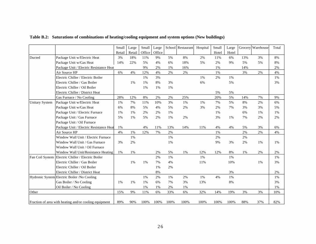
Table B.2: Saturations of combinations of heating/cooling equipment and system options (New buildings)

Small Large Small Large School Restaurant Hospital Small Large Grocery Warehouse TotalRetail Retail Office Office Hotel Hotel

Ducted Package Unit w/Electric Heat 3% 18% 11% 9% 5% 8% 2% 11% 6% 13% 3% 8%Package Unit w/Gas Heat 14% 22% 5% 4% 6% 18% 5% 2% 9% 5% 5% 8%Package Unit / Electric Resistance Heat 9% 2% 1% 16% 1% 14% 2%Air Source HP 6% 4% 12% 4% 2% 2% 1% 3% 2% 4%Electric Chiller / Electric Boiler 1% 3% 1% 2% 1% 1%Electric Chiller / Gas Boiler 1% 1% 8% 3% 6% 5% 3%Electric Chiller / Oil Boiler 1% 1% 1% Electric Chiller / District Heat 5% 5% Gas Furnace / No Cooling 28% 12% 8% 2% 2% 25% 20% 5% 14% 7% 9%

Unitary System Package Unit w/Electric Heat 1% 7% 11% 10% 3% 1% 1% 7% 5% 8% 2% 6%Package Unit w/Gas Heat 6% 8% 5% 4% 5% 2% 3% 2% 7% 3% 3% 5%Package Unit / Electric Furnace 1% 1% 2% 2% 1% 1% 6% 1% 1%Package Unit / Gas Furnace 5% 1% 5% 2% 1% 2% 3% 1% 7% 2% 2%Package Unit / Oil Furnace Package Unit / Electric Resistance Heat 1% 4% 11% 13% 14% 11% 4% 4% 5% 3% 6%Air Source HP 4% 1% 12% 7% 2% 1% 2% 2% 4%Window Wall Unit / Electric Furnace 1% 1% 2% 2% Window Wall Unit / Gas Furnace 3% 2% 1% 9% 3% 2% 1% 1%Window Wall Unit / Oil Furnace Window Wall Unit/Resistance Heating 1% 1% 2% 5% 1% 12% 12% 8% 1% 2% 2%

Fan Coil System Electric Chiller / Electric Boiler 2% 1% 1% 1% 1%Electric Chiller / Gas Boiler 1% 1% 7% 4% 11% 10% 1% 3%Electric Chiller / Oil Boiler 1% 2% Electric Chiller / District Heat 8% 3% 2%

Hydronic System Electric Boiler /No Cooling 1% 2% 1% 2% 1% 4% 1% 1%Gas Boiler / No Cooling 1% 1% 1% 6% 7% 3% 13% 8% 3%Oil Boiler / No Cooling 1% 1% 2% 1% 1%

Other 15% 9% 11% 6% 33% 6% 32% 14% 19% 3% 3% 10%

Fraction of area with heating and/or cooling equipment 89% 90% 100% 100% 100% 100% 100% 100% 100% 88% 37% 82%

2 6

27

APPENDIX C: EFFICIENCY DATA FOR HVAC PLANT OPTIONS

Given the building loads, effect of distribution system type on loads and electricity use, andequipment saturations, energy use can be calculated if the typical plant efficiencies are known. Theloads within the methodology of this report are annual. Therefore, we are interested in efficiencyparameters which would convert annual loads to annual energy use. Seasonal plant heating andcooling efficiencies taken from Sezgen et al. (1995)1 are presented in Table C.1 . These areintegrated part load efficiencies and therefore can be directly used to convert annual loads to annualenergy. Integrated part load efficiencies are generally less than efficiency measured under full loadconditions. Efficiencies were developed both for stock and new equipment.

For combined heating/cooling equipment, there generally exists a secondary heating option whichis utilized if and when the heating requirements are extreme. Efficiencies for these secondaryfeatures are also presented in Table C.1.

1 Sezgen, Osman, Ellen M. Franconi, Jonathan G. Koomey, Steve E. Greenberg, Asim Afzal, and Leslie Shown.1995. Technology Data Characterizing Space Conditioning in Commercial Buildings: Application to End-UseForecasting with COMMEND 4.0. LBL-37065. Lawrence Berkeley National Laboratory, Berkeley, CA. December.

Table C.1: Seasonal Heating and Cooling-Plant Efficiency Data (*)

Seasonal Heating Plant Efficiency (BTU out/BTU in)Average Marginal

Plant Type (stock) (new const.) NotesHEATING

Electric Resistance 1.0 1.0 1Electric Furnace 0.93 0.96 2

Electric Boiler 0.94 0.94 3

Gas Furnace, Typical 0.63 0.76 4Gas Furnace Efficient 0.85 0.89 5

Gas Boiler, Typical 0.6 0.65 6Gas Boiler Efficient 0.85 0.9 7

Oil Furnace 0.68 0.77 8Oil Boiler 0.6 0.68 9

Seasonal Plant Efficiency or COP (BTU out/BTU in) Primary Heating Secondary Heating CoolingAverage Marginal Average Marginal Average Marginal

Plant Type (stock) (new const.) (stock) (new const.) (stock) (new const.) NotesCOMBINED

Electric Packaged 0.93 0.96 n.a. n.a. 2.2 2.7 10Air-Source HP, Std. 2.4 3 0.93 0.96 2.2 2.7 11

Air-Source HP, Effic. 2.8 3.2 0.93 0.96 2.5 3 12Dual-Fuel HP 2.8 3.2 0.63 0.76 2.5 3 13

Water-Loop HP 3.5 4 n.a. n.a. 2.6 3.5 14Gas Packaged 0.7 0.8 n.a. n.a. 2.2 2.7 15

Seasonal Cooling Plant COP (BTU out/BTU in)Average Marginal

Plant Type (stock) (new const.) NotesCOOLINGCentrifugal Chillers:

w/tower 3.5 4.5 16w/evap. condenser 3.8 4.8 17

Reciprocating Chillers:w/air-cooled cond. 2.3 3 18

w/tower 3.4 4 19w/evap. condenser 3.7 4.4 20

Screw Chillers:w/tower 3.7 3.9 21

w/evap. condenser 4 4.2 22

Gas Chiller 0.5 0.9 23

Window/Wall Unit 2.2 2.7 24

28

Sources: [1] Usibelli, A., S. Greenberg, M. Meal, A. Mitchell, R. Johnson, G. Sweitzer, F. Rubinstein, D. Arasteh. 1985. Commercial Conservation Technologies. LBL-18543, Lawrence Berkeley National Laboratory, Berkeley, CA.[2] Electric Power Research Institute. 1992. TAG Technical Assessment Guide, Volume 2: Electricity End Use, Part 2: Com Electricity Use. Electric Power Research Institute, Palo Alto, CA.[3] Electric Power Research Institute. 1989. Handbook of High-Efficiency Electric Equipment and Cogeneration System Op Commercial Buildings. CU-6661. Electric Power Research Institute, Palo Alto, CA.[4] Boiler Efficiency Institute. 1988. Boiler Efficiency Improvement. Boiler Efficiency Institute, Auburn, AL.[5] E-Source. 1992. Space Cooling and Air Handling. E-Source, Inc., Boulder, CO.

Notes:(*) Table reflects the effects of EPACT Standards which affect gas furnaces and boilers, packaged units and heat pumps.1. Assumes that resistance heater and electrical wiring are in space to be heated, so all heat beyond electric meter is useful.2. Average assumes 2% loss from furnace housing and 5% duct leakage to/from unheated space. Marginal assumes 1% and 3. Assumes 2% of rated input is lost through boiler shell; average boiler load is 33%.4. Average assumes 70% seasonal burner efficiency, less 1% each for pilot lights and shell losses and 5% for duct losses; marginal assumes 80%, no pilot, 1% shell, and 3% duct loss.5. Average assumes 90% Calif. Seasonal Efficiency (rather than AFUE, since CSE accounts for fan energy) less 5% duct los marginal same except 92% CA Seasonal Effic., 3% duct loss.6. Average assumes boiler at 80% new steady-state efficiency degraded by 5% due to water and fire-side rust, scale, and soo 2% of input rating lost through boiler casing, 3% through stack; two boilers kept hot all year, average boiler load is 33% o Marginal same except no rust, soot, or scale.7. Average assumes condensing boiler used, but heat exchangers not large enough to lower return water to condensing tempe Marginal assumes condensing boiler used, heat exchangers allow condensing.8. Average assumes 5% better than gas furnace (due to powered burner with controlled excess air and off-cycle air); marginal 1% more efficient than marginal gas (both have power burner or induced draft).9. Average assumed same as gas. Marginal assumes 83% efficiency with the reductions which apply to marginal gas. Oil boilers have more efficiency degradation due to soot, but all have forced or induced draft; effects are assumed to cance10. Electric packaged means direct expansion air conditioner with air-cooled condenser and resistance heat. Heating efficien same as electric furnace. Cooling: Average from [1], [2], and [3]; marginal assumed 0.5 COP point (absolute) higher.11. Primary heating from [2] and [3]; secondary same as electric furnace. Cooling same as electric packaged.12. Primary heating from [2] and [3]; secondary same as electric furnace. Cooling from [3].13. Dual fuel HP means direct expansion cooling and heating with refrigerant-to-air outdoor coil; gas backup. Heat pump C assumed same as effic. air-source; gas effic. assumed same as std. gas furnace. 14. Numbers are from [2] and [3]; averaged assumed to be at lower end of range of most-common COPs; marginal at upper 15. From [3]: cooling same as electric packaged; heating at lower end of range of conventional and effic. units to account fo16. From EPRI and [5]. Approx. 0.1 points of COP reduction for tower fan and condensing water pump; degradation from fo approx. balances improved efficiency at part load. Marginal assumes mid-range of high-effic. equip.17. Same as with tower except about 0.3 point of COP increase for the evaporative condenser. Based on [5].18. From [2] and [3]. Average assumes COP of 3.3 less 0.8 for fans and 0.2 for wear and fouling degradation. Marginal assu above average (approx. diff. between conventional and high efficiency).19. From EPRI and [1]. Assumed 0.1 points of COP reduction (for tower and pump) in mid-range conventional COP for ave same for high-efficiency for marginal.20. Assumes 10% COP improvement for evaporative condenser.21. From [3], using upper end of ranges of conv. and high-effic. less 0.1% for tower and pump. 22. Same as screw with tower except 10% COP improvement with evap. condenser.23. Average assumes 0.6 COP (single-effect); marginal assumes 1.0 COP (double-effect); discounted for tower and pump us24. Assumed same as electric packaged unit. While window/wall units are smaller, they borrow from the more efficient resid

29