Interactive Physically-based Sound Simulation

Nikunj Raghuvanshi

A dissertation submitted to the faculty of the University of North Carolina at ChapelHill in partial fulfillment of the requirements for the degree of Doctor of Philosophy inthe Department of Computer Science.

Chapel Hill2010

Approved by:

Ming C. Lin, Advisor

John Snyder, Reader

Dinesh Manocha, Reader

Gary Bishop, Reader

Marc Niethammer, Reader

c○ 2010

Nikunj Raghuvanshi

ALL RIGHTS RESERVED

ii

AbstractNikunj Raghuvanshi: Interactive Physically-based Sound Simulation.

(Under the direction of Ming C. Lin.)

The realization of interactive, immersive virtual worlds requires the ability to present

a realistic audio experience that convincingly compliments their visual rendering. Phys-

ical simulation is a natural way to achieve such realism, enabling deeply immersive

virtual worlds. However, physically-based sound simulation is very computationally ex-

pensive owing to the high-frequency, transient oscillations underlying audible sounds.

The increasing computational power of desktop computers has served to reduce the

gap between required and available computation, and it has become possible to bridge

this gap further by using a combination of algorithmic improvements that exploit the

physical, as well as perceptual properties of audible sounds. My thesis is a step in this

direction.

My dissertation concentrates on developing real-time techniques for both sub-problems

of sound simulation: synthesis and propagation. Sound synthesis is concerned with gen-

erating the sounds produced by objects due to elastic surface vibrations upon interaction

with the environment, such as collisions. I present novel techniques that exploit human

auditory perception to simulate scenes with hundreds of sounding objects undergoing

impact and rolling in real time. Sound propagation is the complementary problem of

modeling the high-order scattering and diffraction of sound in an environment as it

travels from source to listener. I discuss my work on a novel numerical acoustic sim-

ulator (ARD) that is hundred times faster and consumes ten times less memory than

a high-accuracy finite-difference technique, allowing acoustic simulations on previously-

intractable spaces, such as a cathedral, on a desktop computer.

Lastly, I present my work on interactive sound propagation that leverages my ARD

iii

simulator to render the acoustics of arbitrary static scenes for multiple moving sources

and listener in real time, while accounting for scene-dependent effects such as low-pass

filtering and smooth attenuation behind obstructions, reverberation, scattering from

complex geometry and sound focusing. This is enabled by a novel compact represen-

tation that takes a thousand times less memory than a direct scheme, thus reducing

memory footprints to fit within available main memory. To the best of my knowledge,

this is the only technique and system in existence to demonstrate auralization of physical

wave-based effects in real-time on large, complex 3D scenes.

iv

To my dearest,

Papa, Mummy, Gunjan di, Vandan di and Pritu

v

Acknowledgments

When I started my dissertation research many years ago, I had the following in my

mind: “do some really useful research, quickly, and graduate.” It took me many years to

realize that “quickly” and “useful research” just do not go together in an applied area of

research. So, while I can assure you that my former wish wasn’t fulfilled, hopefully, after

reading this thesis, you would feel that the latter was. I owe a great deal of gratitude

to so many people who have helped me in various ways in my doctoral studies, that I

am sure to miss many of them. To all of them, my apologies for the omission, and my

sincerest, heartfelt thanks for all of your much-needed help.

I thank Ming C. Lin for being a great advisor and helping me guide my efforts

productively through all these years, giving me the freedom to choose my own direction,

leaving me on my own when I was trying to dig into my chosen research direction,

pushing me when I needed to get publications done and promoting my work tirelessly.

And quite importantly, keeping up with my night owl schedule, staying up at nights

many times to help me meet deadlines. My sincerest thanks to her.

I am grateful to Dinesh Manocha for his early support when I started as a graduate

student and his much-needed help in getting me quickly into hands-down research. He

has also been a very helpful committee member. I am especially indebted to Naga

Govindaraju, who mentored me in my first year as a graduate student as well as later

when I was interning in his group at Microsoft Research. He has been a great manager,

mentor and friend. I extend gratitude to Gary Bishop and Marc Niethammer for their

valuable feedback as my committee members.

Also, many thanks to the fellow students in the GAMMA group, who were always

vi

there for interesting discussions, research or otherwise, many of whom are good friends,

some of whom are collaborators too: Jason Sewall, Nico Galoppo, Brandon Lloyd, Rahul

Narain, Sachin Patil, Anish Chandak, Micah Taylor, Abhinav Golas and Sean Curtis. I

am very sure I am missing many people in this list.

I thank the Computer Science staff, because of whose presence, I was able to stay

careless about so many of those practical details that are quite important. They helped

me enjoy the freedom of an irresponsible life a little bit longer. Special thanks goes to

Janet Jones, who was always patient and helpful in the face of all such transgressions.

I would like to thank Ritesh Kumar and Shantanu Sharma, who were my roommates

for nearly four years, during which we had the time of our lives. I am especially indebted

to Ritesh. He is a dear friend and we spent countless hours over coffee discussing

everything from religion and government to computer science, which was, and continues

to be, a richly rewarding experience.

I worked with John Snyder at Microsoft Research during the last year of my doctoral

work and he has provided me with great mentoring, technical help, and objective, bal-

anced criticism for my work. I have learned a lot from his sincere, thorough approach

to research and I am certain he has helped me become a better scientist. My sincerest

thanks to him. I also thank my collaborators from Microsoft Game Studios: Guy Whit-

more and Kristofor Mellroth. As audio directors, they were instrumental in giving my

thesis a more grounded approach based on their expert knowledge of the requirements

of video games. They have also been key in pushing technology based on my work into

real games.

The most I owe is to my parents. What they have done for me extends far beyond

just my doctoral studies. I will just humbly note the one lesson they’ve taught me that

has been the most invaluable in my doctoral studies: Be aware of the practical realities

of the world, but always follow your own compass. It helped me risk choosing my own

topic, and working hard and sincerely on making something useful, even if it meant

vii

having to work harder than just meeting the bar. This has helped shape me into a

better person and a better scientist.

Most importantly, I would like to thank my dear wife, Priti. She was there with me

all through the toughest part of my PhD: the end. She showed tremendous patience

when I was stressed (which was nearly all the time). She was loving when I was careless.

And most importantly, she was always there for me , ensconcing my stress-ridden life in

her calmness. Thank you, Pritu.

viii

Table of Contents

List of Tables . . . . . . . . . . . . . . . . . . . . . . . . . . . . . . . . . . xiii

List of Figures . . . . . . . . . . . . . . . . . . . . . . . . . . . . . . . . . . xiv

1 Introduction . . . . . . . . . . . . . . . . . . . . . . . . . . . . . . . . . 1

1.1 The Quest for Immersion . . . . . . . . . . . . . . . . . . . . . . . . . . . 11

1.2 Physically-based Simulation of Sound . . . . . . . . . . . . . . . . . . . . 16

1.3 Thesis Statement . . . . . . . . . . . . . . . . . . . . . . . . . . . . . . . 18

1.4 Challenges and Contributions . . . . . . . . . . . . . . . . . . . . . . . . 19

1.4.1 Interactive Sound Synthesis . . . . . . . . . . . . . . . . . . . . . 25

1.4.2 Efficient Numerical Acoustics . . . . . . . . . . . . . . . . . . . . 27

1.4.3 Interactive Sound Propagation . . . . . . . . . . . . . . . . . . . . 33

1.5 Thesis Organization . . . . . . . . . . . . . . . . . . . . . . . . . . . . . . 41

2 Previous Work . . . . . . . . . . . . . . . . . . . . . . . . . . . . . . . . 42

2.1 Interactive Sound Synthesis . . . . . . . . . . . . . . . . . . . . . . . . . 45

2.2 Interactive Sound Propagation . . . . . . . . . . . . . . . . . . . . . . . . 49

2.2.1 Acoustic Simulation . . . . . . . . . . . . . . . . . . . . . . . . . 52

2.2.2 Auralization . . . . . . . . . . . . . . . . . . . . . . . . . . . . . . 61

3 Interactive Sound Synthesis . . . . . . . . . . . . . . . . . . . . . . . . 66

3.1 Methodology . . . . . . . . . . . . . . . . . . . . . . . . . . . . . . . . . 66

3.1.1 Input Processing . . . . . . . . . . . . . . . . . . . . . . . . . . . 68

3.1.2 Deformation Modeling . . . . . . . . . . . . . . . . . . . . . . . . 68

ix

3.1.3 Handling Impulsive Forces . . . . . . . . . . . . . . . . . . . . . . 70

3.2 Real-time Sound Synthesis . . . . . . . . . . . . . . . . . . . . . . . . . . 71

3.2.1 Mode Compression . . . . . . . . . . . . . . . . . . . . . . . . . . 73

3.2.2 Mode Truncation . . . . . . . . . . . . . . . . . . . . . . . . . . . 76

3.2.3 Quality Scaling . . . . . . . . . . . . . . . . . . . . . . . . . . . . 78

3.2.4 Putting Everything Together . . . . . . . . . . . . . . . . . . . . . 79

3.3 Implementation and Results . . . . . . . . . . . . . . . . . . . . . . . . . 81

3.3.1 Rigid Body Simulation . . . . . . . . . . . . . . . . . . . . . . . . 81

3.3.2 Position Dependent Sounds . . . . . . . . . . . . . . . . . . . . . 83

3.3.3 Rolling Sounds . . . . . . . . . . . . . . . . . . . . . . . . . . . . 83

3.3.4 Efficiency . . . . . . . . . . . . . . . . . . . . . . . . . . . . . . . 85

3.4 Conclusion and Future Work . . . . . . . . . . . . . . . . . . . . . . . . . 86

4 Efficient Numerical Acoustics . . . . . . . . . . . . . . . . . . . . . . . 89

4.1 Mathematical Background . . . . . . . . . . . . . . . . . . . . . . . . . . 89

4.1.1 Basic Formulation . . . . . . . . . . . . . . . . . . . . . . . . . . . 90

4.1.2 A (2,6) FDTD Scheme . . . . . . . . . . . . . . . . . . . . . . . . 91

4.1.3 Numerical Dispersion in FDTD and Efficiency Considerations . . 92

4.1.4 Wave Equation on a Rectangular Domain . . . . . . . . . . . . . 93

4.2 Technique . . . . . . . . . . . . . . . . . . . . . . . . . . . . . . . . . . . 96

4.2.1 Adaptive Rectangular Decomposition . . . . . . . . . . . . . . . . 98

4.2.2 Interface Handling . . . . . . . . . . . . . . . . . . . . . . . . . . 99

4.2.3 Domain Decompositon Method and ARD . . . . . . . . . . . . . . 100

4.2.4 Absorbing Boundary Condition . . . . . . . . . . . . . . . . . . . 103

4.2.5 Putting everything together . . . . . . . . . . . . . . . . . . . . . 104

4.2.6 Numerical Errors . . . . . . . . . . . . . . . . . . . . . . . . . . . 104

x

4.2.7 ARD and FDTD: efficiency comparison . . . . . . . . . . . . . . . 107

4.3 Results . . . . . . . . . . . . . . . . . . . . . . . . . . . . . . . . . . . . . 110

4.3.1 Offline Sound Rendering . . . . . . . . . . . . . . . . . . . . . . . 110

4.3.2 Numerical Dispersion: Anechoic Corridor . . . . . . . . . . . . . . 114

4.3.3 House Scene . . . . . . . . . . . . . . . . . . . . . . . . . . . . . . 115

4.3.4 Cathedral Scene . . . . . . . . . . . . . . . . . . . . . . . . . . . . 116

4.4 Conclusion and Future Work . . . . . . . . . . . . . . . . . . . . . . . . . 117

5 Interactive Sound Propagation . . . . . . . . . . . . . . . . . . . . . . 121

5.1 Perception in Acoustic Spaces . . . . . . . . . . . . . . . . . . . . . . . . 122

5.1.1 Early Reflections (ER) . . . . . . . . . . . . . . . . . . . . . . . . 123

5.1.2 Late Reverberation (LR) . . . . . . . . . . . . . . . . . . . . . . . 124

5.2 Acoustic Precomputation . . . . . . . . . . . . . . . . . . . . . . . . . . . 125

5.2.1 Numerical Simulation . . . . . . . . . . . . . . . . . . . . . . . . . 126

5.2.2 LR Processing . . . . . . . . . . . . . . . . . . . . . . . . . . . . . 128

5.2.3 ER Processing . . . . . . . . . . . . . . . . . . . . . . . . . . . . . 130

5.3 Interactive Auralization Runtime . . . . . . . . . . . . . . . . . . . . . . 135

5.3.1 Load-time Computation . . . . . . . . . . . . . . . . . . . . . . . 135

5.3.2 ERIR Interpolation . . . . . . . . . . . . . . . . . . . . . . . . . . 136

5.3.3 LRIR Scaling . . . . . . . . . . . . . . . . . . . . . . . . . . . . . 138

5.3.4 Binaural Processing . . . . . . . . . . . . . . . . . . . . . . . . . . 139

5.3.5 ERIR Short Fourier Transform . . . . . . . . . . . . . . . . . . . 139

5.3.6 Auralization . . . . . . . . . . . . . . . . . . . . . . . . . . . . . . 140

5.4 Implementation and Results . . . . . . . . . . . . . . . . . . . . . . . . . 141

5.4.1 Living room . . . . . . . . . . . . . . . . . . . . . . . . . . . . . . 144

5.4.2 Walkway . . . . . . . . . . . . . . . . . . . . . . . . . . . . . . . . 144

xi

5.4.3 Citadel . . . . . . . . . . . . . . . . . . . . . . . . . . . . . . . . . 145

5.4.4 Train station . . . . . . . . . . . . . . . . . . . . . . . . . . . . . 146

5.4.5 Error Analysis . . . . . . . . . . . . . . . . . . . . . . . . . . . . . 146

5.4.6 “Shoebox” Experimental Results . . . . . . . . . . . . . . . . . . 150

5.5 Conclusion, Limitations and Future Work . . . . . . . . . . . . . . . . . 151

6 Conclusion and Future Work . . . . . . . . . . . . . . . . . . . . . . . 153

Bibliography . . . . . . . . . . . . . . . . . . . . . . . . . . . . . . . . . . . 158

xii

List of Tables

4.1 FLOPS comparison of FDTD vs ARD on a scene of volume V = 10, 000m3

with maximum simulation frequency vmax = 1kHz for the duration t = 1sec. Theoretically, ARD which uses samples per wavelength, s = 2.6, isnearly hundred times efficient than FDTD (s = 10) on account of using amuch coarser grid. The value of “FLOPS per cell” is defined as the ratioof the total FLOPS and N , the total number of cells. . . . . . . . . . . . 109

5.1 Performance statistics. Tables (a) and (b) show performance numbersfor precomputation and runtime stages, respectively, for the four differentscenes used for auralization tests. Abbreviated column headings are asfollows. Precomputation: “Dim.” is the scene dimensions. “#ERL”is the simulated number of ER listener probes (before downsampling).“#ERS” is the simulated number of ER source probes. “#R” is thenumber of rooms in the scene. “ST” is total simulation time, includingLR and ER probes. Runtime: “Mem.” is the total memory used forall source and receiver positions, including extracted peaks and frequencytrend. TER is the length of the ER phase, and TLR the LR phase, maxi-mized over all rooms in the scene. “#S” is the number of different sourcessimulated at run-time. “ABT” is the total time needed to process eachaudio buffer, summed over all run-time sources. . . . . . . . . . . . . . . 142

xiii

List of Figures

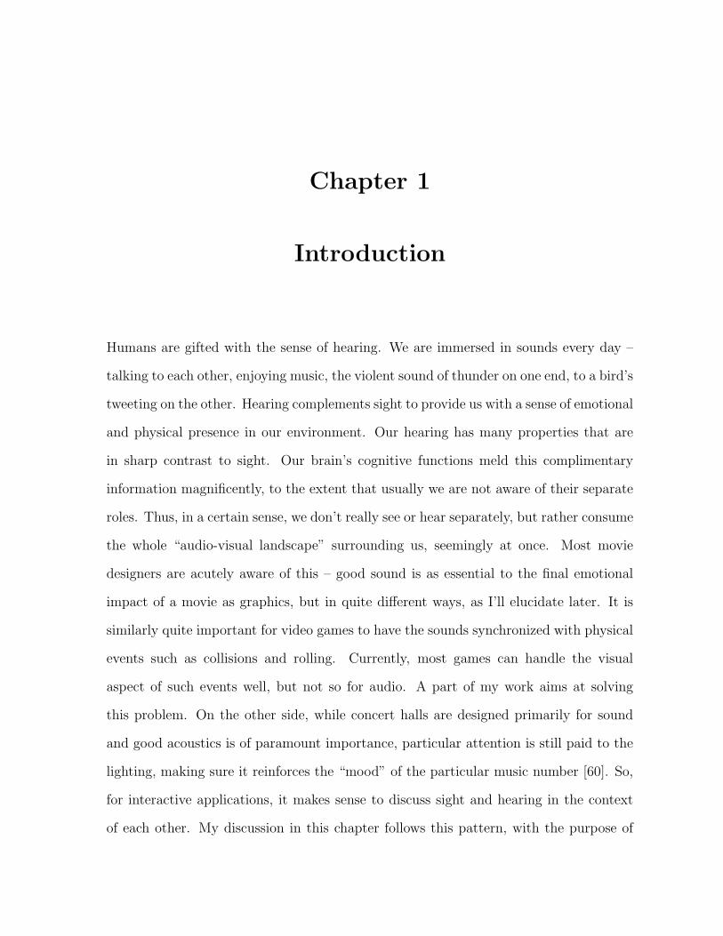
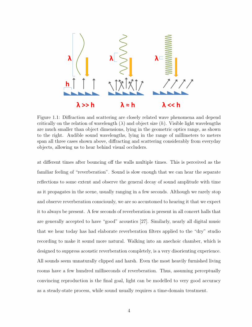
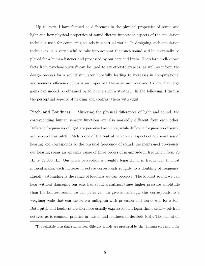
1.1 Diffraction and scattering are closely related wave phenomena and de-pend critically on the relation of wavelength (λ) and object size (h).Visible light wavelengths are much smaller than object dimensions, ly-ing in the geometric optics range, as shown to the right. Audible soundwavelengths, lying in the range of millimeters to meters span all threecases shown above, diffracting and scattering considerably from everydayobjects, allowing us to hear behind visual occluders. . . . . . . . . . . . 4

1.2 A screenshot from the game Half Life 2: Lost Coast illustrating the visualrealism achievable with games today. . . . . . . . . . . . . . . . . . . . . 12

1.3 Numerous dice fall on a three-octave xylophone in close succession, play-ing out the song “The Entertainer”. Please go to http://gamma.cs.unc.edu/symphony to see and hear the xylophone playing. . . . . . . . . . . . 24

1.4 Sound simulation on a Cathedral. The dimensions of this scene are35m × 15m × 26m. My technique is able to perform numerical soundsimulation on this complex scene on a desktop computer and precomputea 1 second long impulse response in about 29 minutes, taking less than1 GB of memory, while the current state-of-the-art FDTD takes a fewdays to perform the same simulation, at high-accuracy settings. Pleasego to http://gamma.cs.unc.edu/propagation to see a video containingauralizations on this scene and other examples. . . . . . . . . . . . . . . 28

1.5 Train station scene from Valve’s SourceTM game engine SDK (http://source.valvesoftware.com). My method performs real-time aural-ization of sounds from dynamic agents, objects and the player inter-acting in the scene, while accounting for perceptually important effectssuch as diffraction, low-pass filtering and reverberation. Please go tohttp://gamma.cs.unc.edu/PrecompWaveSim to see a video containingauralizations on this scene and other examples. . . . . . . . . . . . . . . 34

3.1 This diagram gives an overview of my sound-synthesis approach. . . . . 67

xiv

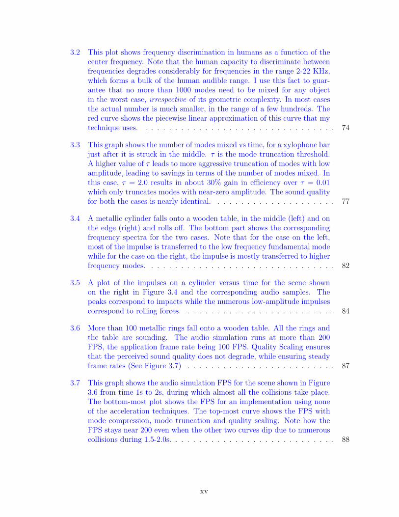
3.2 This plot shows frequency discrimination in humans as a function of thecenter frequency. Note that the human capacity to discriminate betweenfrequencies degrades considerably for frequencies in the range 2-22 KHz,which forms a bulk of the human audible range. I use this fact to guar-antee that no more than 1000 modes need to be mixed for any objectin the worst case, irrespective of its geometric complexity. In most casesthe actual number is much smaller, in the range of a few hundreds. Thered curve shows the piecewise linear approximation of this curve that mytechnique uses. . . . . . . . . . . . . . . . . . . . . . . . . . . . . . . . . 74

3.3 This graph shows the number of modes mixed vs time, for a xylophone barjust after it is struck in the middle. τ is the mode truncation threshold.A higher value of τ leads to more aggressive truncation of modes with lowamplitude, leading to savings in terms of the number of modes mixed. Inthis case, τ = 2.0 results in about 30% gain in efficiency over τ = 0.01which only truncates modes with near-zero amplitude. The sound qualityfor both the cases is nearly identical. . . . . . . . . . . . . . . . . . . . . 77

3.4 A metallic cylinder falls onto a wooden table, in the middle (left) and onthe edge (right) and rolls off. The bottom part shows the correspondingfrequency spectra for the two cases. Note that for the case on the left,most of the impulse is transferred to the low frequency fundamental modewhile for the case on the right, the impulse is mostly transferred to higherfrequency modes. . . . . . . . . . . . . . . . . . . . . . . . . . . . . . . . 82

3.5 A plot of the impulses on a cylinder versus time for the scene shownon the right in Figure 3.4 and the corresponding audio samples. Thepeaks correspond to impacts while the numerous low-amplitude impulsescorrespond to rolling forces. . . . . . . . . . . . . . . . . . . . . . . . . . 84

3.6 More than 100 metallic rings fall onto a wooden table. All the rings andthe table are sounding. The audio simulation runs at more than 200FPS, the application frame rate being 100 FPS. Quality Scaling ensuresthat the perceived sound quality does not degrade, while ensuring steadyframe rates (See Figure 3.7) . . . . . . . . . . . . . . . . . . . . . . . . . 87

3.7 This graph shows the audio simulation FPS for the scene shown in Figure3.6 from time 1s to 2s, during which almost all the collisions take place.The bottom-most plot shows the FPS for an implementation using noneof the acceleration techniques. The top-most curve shows the FPS withmode compression, mode truncation and quality scaling. Note how theFPS stays near 200 even when the other two curves dip due to numerouscollisions during 1.5-2.0s. . . . . . . . . . . . . . . . . . . . . . . . . . . . 88

xv

4.1 Numerical dispersion with a (2,6) FDTD scheme for different mesh reso-lutions. Increasing the sampling reduces the numerical dispersion errors.Our method suffers from no dispersion errors in the interior of rectan-gular partitions, while FDTD accumulates errors over each cell a signalpropagates across. Reducing these errors with FDTD requires a very finegrid. . . . . . . . . . . . . . . . . . . . . . . . . . . . . . . . . . . . . . . 93

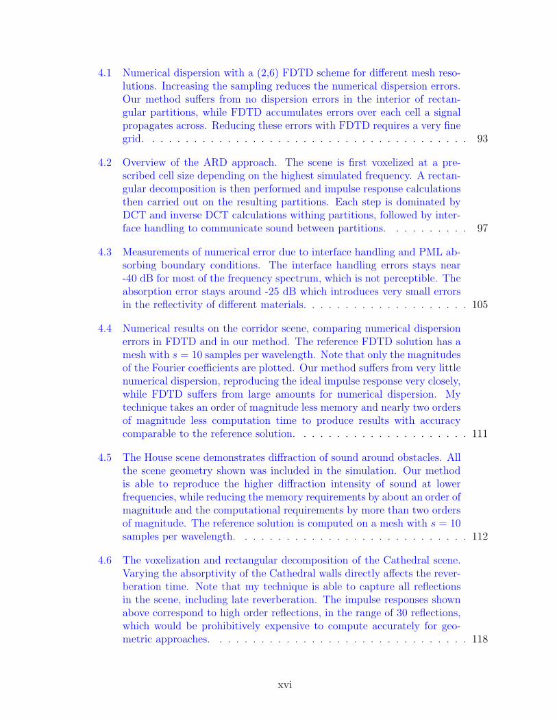
4.2 Overview of the ARD approach. The scene is first voxelized at a pre-scribed cell size depending on the highest simulated frequency. A rectan-gular decomposition is then performed and impulse response calculationsthen carried out on the resulting partitions. Each step is dominated byDCT and inverse DCT calculations withing partitions, followed by inter-face handling to communicate sound between partitions. . . . . . . . . . 97

4.3 Measurements of numerical error due to interface handling and PML ab-sorbing boundary conditions. The interface handling errors stays near-40 dB for most of the frequency spectrum, which is not perceptible. Theabsorption error stays around -25 dB which introduces very small errorsin the reflectivity of different materials. . . . . . . . . . . . . . . . . . . . 105

4.4 Numerical results on the corridor scene, comparing numerical dispersionerrors in FDTD and in our method. The reference FDTD solution has amesh with s = 10 samples per wavelength. Note that only the magnitudesof the Fourier coefficients are plotted. Our method suffers from very littlenumerical dispersion, reproducing the ideal impulse response very closely,while FDTD suffers from large amounts for numerical dispersion. Mytechnique takes an order of magnitude less memory and nearly two ordersof magnitude less computation time to produce results with accuracycomparable to the reference solution. . . . . . . . . . . . . . . . . . . . . 111

4.5 The House scene demonstrates diffraction of sound around obstacles. Allthe scene geometry shown was included in the simulation. Our methodis able to reproduce the higher diffraction intensity of sound at lowerfrequencies, while reducing the memory requirements by about an order ofmagnitude and the computational requirements by more than two ordersof magnitude. The reference solution is computed on a mesh with s = 10samples per wavelength. . . . . . . . . . . . . . . . . . . . . . . . . . . . 112

4.6 The voxelization and rectangular decomposition of the Cathedral scene.Varying the absorptivity of the Cathedral walls directly affects the rever-beration time. Note that my technique is able to capture all reflectionsin the scene, including late reverberation. The impulse responses shownabove correspond to high order reflections, in the range of 30 reflections,which would be prohibitively expensive to compute accurately for geo-metric approaches. . . . . . . . . . . . . . . . . . . . . . . . . . . . . . . 118

xvi

5.1 Impulse response (IR) and corresponding frequency response(FR) for a simple scene with one reflection. . . . . . . . . . . . . . . . . 123

5.2 IR encoding. The late reverberation (LR) filter is stored once per room.The early reflections (ER) filter is represented as a set of peaks and afrequency trend, and stored at each source/listener grid point. . . . . . . 130

5.3 Run-time processing. Operations computed at run-time are coloredred. Processing for only one channel (ear) is shown at figure bottom. . . 136

5.4 Scenes used for auralization tests. . . . . . . . . . . . . . . . . . . . . . . 138

5.5 Sound scattering and diffusion in the living room scene. Thetop row shows an empty room while the bottom row is fully-furnished.The left three columns show a 2D slice of the sound field generated by aGaussian impulse emitted near the room’s center, while the right columnshows the entire IR at a single receiver point placed at the source location.Red/blue represents positive/negative pressure in the sound field. Blackareas represent solid geometry in the scene. Note the large difference inwave propagation in the two scenes because of scattering and diffraction.Refer to the video (link given in Section 5.4) for comparative auralizations. 143

5.6 Error analysis of my technique in the living room scene, at thesource/listener points shown on the left. The top graph isolates errorsfrom IR parametrization (peaks and frequency trend) alone, while thebottom graph accounts for interpolation as well, at a point midway be-tween listener samples (red dots on left). The error between the approx-imated response with my technique and the reference appears in the toppart of each plot. The bottom graph also compares linear interpolation(green curve) against my method (black curve). Linear interpolation pro-duces more error overall and incorrectly attenuates higher frequencies.. . . . . . . . . . . . . . . . . . . . . . . . . . . . . . . . . . . . . . . . . 145

5.7 Error analysis compared to broadband numerical simulation:listener close to source. My method matches the reference solutionvery closely, while linear interpolation yields substantial errors. . . . . . 147

5.8 Error analysis compared to broadband numerical simulation:listener on couch. Compression error stays around 2dB till 1kHz andthen increases to 4dB at 4kHz. Linear interpolation produces much moreerror. . . . . . . . . . . . . . . . . . . . . . . . . . . . . . . . . . . . . . 148

xvii

5.9 Error analysis compared to broadband numerical simulation:listener outside door. Sound from the source undergoes multiple scat-tering in the room, then diffracts around the door to arrive at the listener.Such high-order effects are very hard to model convincingly and a chal-lenging case for current systems. Notice the clear low-pass filtering in thefrequency response plotted and audible in the demo. Compression errorlies between 2 to 4 dB, which is quite low. Spatial interpolation errorsare higher, crossing 5 dB, but my technique produces less error over allfrequencies than linear interpolation. . . . . . . . . . . . . . . . . . . . . 149

5.10 Effect of atmospheric attenuation. Results for the Image Sourcemethod on a simple “shoebox” geometry shown in the upper-right insetare plotted on the left. Impulse responses were calculated assuming afrequency-independent pressure absorption coefficient of 0.15 at the roomwalls, but with frequency-dependent atmospheric attenuation using theformulae given in ISO 9613-1 assuming an air temperature of 20◦C andrelative humidity of 40%. The spectrogram on the right shows strongattenuation of frequencies above 5kHz. In particular, a 10kHz soundcomponent decays by nearly 20 dB after just 200 ms of propagation.In a real scene where frequency-dependent material absorption is alsoaccounted for, the attenuation would be even higher. . . . . . . . . . . . 150

5.11 Error analysis compared with Image Source method. The left im-age shows the locations of source and listener in a simple “shoebox” room.A reference 200 ms long IR was generated with the Image Source method.The resulting frequency response is compared with my technique’s resultbased on a wave simulation bandlimited to 1kHz, and including com-pression and spatial interpolation errors. The result obtained with mytechnique (red curve) agrees well with the reference solution. In the toperror plot, maximum error is about 5 dB while average error over the fullfrequency range up to 16kHz is 2-3 dB. Linear interpolation (green curve)yields larger errors and incorrectly attenuates higher frequencies. . . . . 151

xviii

Chapter 1

Introduction

Humans are gifted with the sense of hearing. We are immersed in sounds every day –

talking to each other, enjoying music, the violent sound of thunder on one end, to a bird’s

tweeting on the other. Hearing complements sight to provide us with a sense of emotional

and physical presence in our environment. Our hearing has many properties that are

in sharp contrast to sight. Our brain’s cognitive functions meld this complimentary

information magnificently, to the extent that usually we are not aware of their separate

roles. Thus, in a certain sense, we don’t really see or hear separately, but rather consume

the whole “audio-visual landscape” surrounding us, seemingly at once. Most movie

designers are acutely aware of this – good sound is as essential to the final emotional

impact of a movie as graphics, but in quite different ways, as I’ll elucidate later. It is

similarly quite important for video games to have the sounds synchronized with physical

events such as collisions and rolling. Currently, most games can handle the visual

aspect of such events well, but not so for audio. A part of my work aims at solving

this problem. On the other side, while concert halls are designed primarily for sound

and good acoustics is of paramount importance, particular attention is still paid to the

lighting, making sure it reinforces the “mood” of the particular music number [60]. So,

for interactive applications, it makes sense to discuss sight and hearing in the context

of each other. My discussion in this chapter follows this pattern, with the purpose of

illustrating the need for better sound simulation in today’s applications and contrasting

it with light simulation to clarify the uniqueness of many of the problems encountered

when trying to create realistic aural experiences on digital computers. This provides

context for the contributions of this thesis.

The differences between sight and hearing begin with our sense organs. We have two

frontally-located eyes with limited field of view and two ears located on diametrically

opposite sides of the head with an unlimited field of view. Our eyes can be opened or

closed at will, but our ears are always “on.” While we sleep, we can still be awoken at

any moment by a loud noise. While eyes don’t differ so drastically in their geometry

from person to person, the shape of our external ears varies substantially, along with our

head and shoulder geometry. All these factors affect how each individual hears sounds

in their environment. We regularly hear things that we can’t see and by combining

both sight and hearing, our mind ensures cognitive continuity even when there is visual

discontinuity. For example, usually we are not startled by people walking around corners,

by heeding the sound of their footsteps as they approach.1 In addition to combining

audio-visual data, our brain also checks for consistency in the common information.

For example, it is disconcerting to have a person visually located in front of you, while

his voice comes from behind. This situation is easily created in a teleconferencing

environment with the screen in front and speakers behind you. The brain cross-references

the location of the other person using both sight and hearing, finds two different results,

leading to cognitive conflict and confusion. Therefore, in order to create a realistic

experience for a user in a virtual world (such as a player in a 3D video game), one has

to pay very close attention that hearing correctly reinforces sight just like in reality. We

will see this pattern reappear many times in this discussion.

The complimentary information that sight and hearing provide to the brain is ul-

1If you think about it, we do get startled in office corridors when the carpet is soft and muffles thefootstep sounds too much.

2

timately based on physics. Our eyes and ears are designed to receive and process two

fundamentally different kinds of physical waves – light and sound, respectively. There-

fore, in order to create a convincingly realistic virtual world, both light and sound are

crucial and a natural way to obtain perceptual realism is to employ “physically-based

modeling” – simulate light and sound using a digital computer by employing well known

physical equations governing the two phenomena. The thrust of this thesis is on efficient

physical simulation of sound. It turns out that the production and propagation mecha-

nisms for the perceivable range of light and sound are vastly different. This underlying

difference in physics governs what simulation methods and approximations work best for

each. In order to motivate why sound simulation poses its unique set of computational

challenges, I discuss below in detail some of the most important physical differences

between sound and light and how they affect the perception of each as well as dictate

the necessary properties a sound simulator must possess in order to be useful. Since

attention is restricted to only the perceivable range of light and sound for the purposes

of my work, in the rest of this document, the terms “light” and “sound” will be assumed

to mean ”visible light” and “audible sound” respectively, unless otherwise stated.

The propagation speed of light and sound are very different. While light consists of

electromagnetic waves that can propagate through vacuum, sound consists of extremely

tiny (about 2/10,000,000,000 of an atmosphere) pressure fluctuations in air. At a speed

of 300,000,000 m/s (meters per second) in vacuum, light travels staggeringly fast com-

pared to sound, which travels at a comparatively slow speed of 340 m/s in air at room

temperature. This causes major perceptual differences in their behavior – when we

switch on a light bulb in a room, the light field reaches steady state in a matter of mi-

croseconds; too fast for us to perceive it while it is bouncing off the walls. Consequently,

we only perceive the steady state light field. In contrast, when a musical instrument

plays in a concert hall, in addition to the sound reaching us directly from the musical

instrument, we also hear (modified) copies of the sound coming from different directions

3

h

λ λ λ

λ >> h λ ≈ h λ << hFigure 1.1: Diffraction and scattering are closely related wave phenomena and dependcritically on the relation of wavelength (λ) and object size (h). Visible light wavelengthsare much smaller than object dimensions, lying in the geometric optics range, as shownto the right. Audible sound wavelengths, lying in the range of millimeters to metersspan all three cases shown above, diffracting and scattering considerably from everydayobjects, allowing us to hear behind visual occluders.

at different times after bouncing off the walls multiple times. This is perceived as the

familiar feeling of “reverberation”. Sound is slow enough that we can hear the separate

reflections to some extent and observe the general decay of sound amplitude with time

as it propagates in the scene, usually ranging in a few seconds. Although we rarely stop

and observe reverberation consciously, we are so accustomed to hearing it that we expect

it to always be present. A few seconds of reverberation is present in all concert halls that

are generally accepted to have “good” acoustics [27]. Similarly, nearly all digital music

that we hear today has had elaborate reverberation filters applied to the “dry” studio

recording to make it sound more natural. Walking into an anechoic chamber, which is

designed to suppress acoustic reverberation completely, is a very disorienting experience.

All sounds seem unnaturally clipped and harsh. Even the most heavily furnished living

rooms have a few hundred milliseconds of reverberation. Thus, assuming perceptually

convincing reproduction is the final goal, light can be modelled to very good accuracy

as a steady-state process, while sound usually requires a time-domain treatment.

4

The perceivable wavelengths of light and sound differ by many orders of magnitude.

Visible light consists of wavelengths in hundreds of nanometers, which is thousands to

millions of times smaller than the size of the objects we deal with usually, lying in

range of millimeters to meters. This falls entirely in the regime shown on the right

side of Figure 1.1 where wave propagation can be safely reduced to the abstraction of

infinitely thin rays propagating in straight lines that undergo local interactions with

object geometry upon intersection. This is called the “geometric approximation” which

underlies techniques such as ray-tracing, and has served quite well for simulating light

transport. Because of the minute wavelength of light, we rarely observe its wave-nature

with the unaided eye, except in very special circumstances. Such examples are the

colored patterns on the surface of a CD or the colored patterns on a bubble’s surface.

In both these cases, the geometric feature size, namely the pits on the surface of the

CD and the width of the bubble surface, is comparable to visible light wavelengths, thus

revealing its wave nature. In complete contrast to light, audible sound has wavelengths

in the range of a few millimeters to a few meters, making wave-related effects ubiquitous.

One of the most important wave phenomena is diffraction, where a wave tends to spread

in space as it propagates and thus bends around obstacles. Because sound wavelengths

are comparable to the size of spaces we live in, diffraction is a common observation

with sound and is integrated in our perception. While we expect sharp visibility events

with light, we are not aware of perceiving any sharp “sound shadows” where a sound

is abruptly cut off behind an obstacle. Rather, it is common experience that loudness

decreases smoothly behind an occluder. As a result, as discussed previously, we can hear

footsteps around a corner. The occlusion effect is more pronounced for higher frequency

components of the sound since they have a shorter wavelength than the lower frequency

components. The net perceptual effect is that, in addition to the the sound getting

gradually fainter, its “shrillness” or “brightness” is also reduced behind obstructions. A

simple experiment demonstrates this effect. Play a white noise sound on the computer

5

and then turn off one of the speakers by shifting the balance to completely left or right.

This ensures that the sound emanates from only one of the speakers. Now bring a thick

obstruction, such as a notepad between yourself and the speaker, making sure that the

speaker is not visible. Remove the obstruction, bring it back, and repeat. You will

notice that the noise is much more bearable when the source is not visible. This effect

is because not only is its loudness reduced but additionally, its overall “shrillness” shifts

lower when obstructed. This shift happens because higher frequency components of the

noise are attenuated much more in relation to lower frequencies. Stated in the language

of signal processing, an obstruction acts like a low-pass filter applied on the source sound

signal. In summary, owing to its extremely small wavelength, light diffracts very little

around common objects with sizes of a few millimeters or larger. Thus, it carries very

precise spatial detail about objects, but on the flip-side, it can be completely stopped by

an obstruction, casting a sharp shadow. Sound behaves in the exactly opposite fashion

because of its much larger wavelength, not conveying spatial details with the precision

of light, but having the ability to propagate and carry useful information into optically

occluded regions. Therefore, geometric approximations (eg. rays, beams, photons) work

well for light, but perceptually convincing sound simulation requires a full wave-based

treatment because of the much larger wavelength of audible sounds. Another important

property of sound is interference.

Interference is a physical property of waves. When two propagating waves overlap in

a region of space, they add constructively or destructively depending on their respective

phases at each point in the region. For example, when a crest and trough overlap

at a point, the waves cancel out. We usually do not observe interference effects for

light because most light sources are incoherent, emitting light with randomized phase.

Thus, the total light intensity at any point in space can be described simply as the

(phase-agnostic) sum of the intensities of all contributions at that point. In contrast,

most sound sources are coherent and interference is quite important for sound. When a

6

wave undergoes multiple scattering in a domain and interferes with itself, it generates

a spatially and temporally varying amplitude pattern called an “interference pattern.”

For specific frequencies that are determined by the vibrating entity’s geometry and

boundary properties, the interference patterns become time-invariant, forming standing

waves. The vibrating entity could be the air column of a flute, the cavity in the wind-pipe

of a vocalist, a string of a piano or even the whole air in a room. This is the phenomenon

of resonance, the effect of which is to selectively amplify specific frequencies, called the

resonant modes. The spatial interference patterns for resonant modes are called the

mode shapes.

Resonance is the physical mechanism behind nearly all musical instruments – they

are designed in such a manner that they resonate at precisely the frequencies of musical

notes so that the energy spent by the musician is guaranteed to translate into the desired

notes. The act of tuning an instrument is meant to align its resonant frequencies to

musical notes. Resonance applies to the whole air in a room as well. Most rooms,

especially those with small dimensions, such as recording studios or living rooms, have

resonant frequencies of their own because sound will reflect and scatter at the walls

and furniture and interfere with itself. The sound emanating from the speakers is thus

modified substantially by the room, and to make matters worse, the interference pattern

is directly audible at lower frequencies so that at some points there is too much “boom”

and at others there is none. Such room resonances create a very inhomogeneous and

undesirable listening experience which needs to be mitigated by moving the listener

position (couch, for example) and/or placing furniture and other scattering geometry

at locations chosen to destroy the standing waves. Thus, while resonance makes life

of the musician easy, and makes it equally tough for the room acoustician. This is

because the musician relies on resonance to generate select (musical) frequencies, and

the room acoustician tries to stop the room from amplifying its own select (resonant)

frequencies, in order to ensure that any music played within the room reaches the listener

7

in essentially the same form as it was radiated from the instrument or loudspeakers.

Thus, any simulation approach for sound must be able to capture interference and the

resulting resonance effects.

Resonance is very closely related to the mathematical technique of “modal analysis”

which has the tremendous advantage of having a direct physical interpretation. Given

the computer model of a vibrating entity along with appropriate boundary conditions,

modal analysis allows one to find all of its resonant modes and their shapes. These

computed resonant modes and shapes correspond directly to their physical counterparts.

Mathematically, it is known that an arbitrary vibration can be expressed as a linear

combination of resonant modes vibrating with different, time-dependent strengths. This

offers substantial computational benefits, as I will describe in detail later. To give

a quick example, given a guitar string’s length, tension, material etc., it is possible to

determine its resonant modes and mode shapes using modal analysis, which is performed

beforehand (precomputed). At runtime, given the position and strength of a pluck, one

can very quickly evaluate the response of the string and the sound it emits by expressing

the pluck strength as well as the resulting vibration as a sum of the resonant mode shapes

oscillating independently at their corresponding mode frequencies.

The dynamic range2 of perceivable frequencies for sound is much larger than

light. We can perceive sounds ranging from 20 to 22,000 Hertz, which is a dynamic

range of roughly one thousand (three orders of magniture). The corresponding range

for visible light is 400 to 800 Terahertz, the dynamic range being just two. The lowest

frequencies of sound propagate very differently from the higher frequencies because of

the large difference in wavelength. This means that sound simulation necessarily has to

be broadband – simulating within a small frequency range doesn’t work in the general

case.

2defined as the ratio of the highest to the lowest values of interest for a physical quantity

8

Up till now, I have focused on differences in the physical properties of sound and

light and how physical properties of sound dictate important aspects of the simulation

technique used for computing sounds in a virtual world. In designing such simulation

techniques, it is very useful to take into account that such sound will be eventually be

played for a human listener and processed by our ears and brain. Therefore, well-known

facts from psychoacoustics3 can be used to set error-tolerances, as well as inform the

design process for a sound simulator hopefully leading to increases in computational

and memory efficiency. This is an important theme in my work and I show that large

gains can indeed be obtained by following such a strategy. In the following, I discuss

the perceptual aspects of hearing and contrast them with sight.

Pitch and Loudness: Mirroring the physical differences of light and sound, the

corresponding human sensory functions are also markedly different from each other.

Different frequencies of light are perceived as colors, while different frequencies of sound

are perceived as pitch. Pitch is one of the central perceptual aspects of our sensation of

hearing and corresponds to the physical frequency of sound. As mentioned previously,

our hearing spans an amazing range of three orders of magnitude in frequency, from 20

Hz to 22,000 Hz. Our pitch perception is roughly logarithmic in frequency. In most

musical scales, each increase in octave corresponds roughly to a doubling of frequency.

Equally astounding is the range of loudness we can perceive. The loudest sound we can

hear without damaging our ears has about a million times higher pressure amplitude

than the faintest sound we can perceive. To give an analogy, this corresponds to a

weighing scale that can measure a milligram with precision and works well for a ton!

Both pitch and loudness are therefore usually expressed on a logarithmic scale – pitch in

octaves, as is common practice in music, and loudness in decibels (dB). The definition

3The scientific area that studies how different sounds are processed by the (human) ears and brain

9

of the decibel scale is as follows –

Loudness (dB) := 10 ∗ log10(I

I0

), (1.1)

where I is the intensity of sound, which is proportional to the square of the pressure

amplitude. The reference intensity, I0 = 10−12 W/m2 corresponds to the lowest audible

sound intensity and evaluates to 0 dB. The pitch and loudness scales mirror our percep-

tion quite well. Each increase in octave increases the pitch by equal amounts. Similarly,

each increase in dB increases the loudness by equal amounts.

Hearing is primarily temporal, sight is spatial: This is the most fundamental dif-

ference between how sight and hearing interact with our cognition. The major function

of human vision is to provide spatial information carried by the light entering our eyes.

Motion is important, but we can resolve temporal events only at roughly 24Hz; inter-

mediate events are fused together to give a smooth feeling of motion. This is exploited

by all computer, TV and movie displays by drawing a quick succession of photographs

at or above an update rate of 24Hz. In comparison, hearing is a truly continuous and

temporal sense. Where sight stops, hearing begins – we hear from 20Hz up to 22,000Hz.

What that implies is that we can directly sense vibrations happening with a period

less than a millisecond with ease. Moreover, any simulation that needs to capture such

vibrations has to have an update rate of at least 44,000Hz. Our sense of hearing is

attuned to the overall frequency content of sound and how this composition changes

over time. This is fundamental to our perception of all the sounds around us, such

as music and speech. Music is almost purely a temporal experience. Using our senses

of sight and hearing together, we observe our surroundings at millimeter resolution in

space and sub-millisecond resolution in time. However, sounds do provide approximate

spatial information that can be essential when visual information is not available and

can help direct our gaze. When someone calls our name from behind we can “localize

10

their voice” (that is, find the direction of their voice) to within a few degrees by utilizing

the microsecond delay, as well as intensity difference between the sound reaching our

ears from the source [10]. However, we cannot deduce the shape of an object from its

sound. In fact, it can be proven mathematically that this is impossible to do[35]. Nor

can we perceive the geometry of a wall from sound scattered from it, as we can for light.

The scattering does produce noticeable differences in the temporal composition of the

final sound due frequency-dependent diffraction, reflection and interference, but it does

not provide the fine-scale geometric information that light provides.

To summarize, the physical behavior of light and sound are very different, so is the

information they provide, so is their perception, and so have to be any techniques

that attempt to simulate them on a digital computer. Light simulation techniques can

usually use steady state simulations in combination with infinite frequency (geometric

optic) approximations that ignore interference, at update rates of 24Hz or higher. In

contrast, perceptually convincing sound simulation requires full-wave, broadband, time-

domain solutions with update rates of 44,000Hz or higher. Additionally, the simulation

techniques much account for interference and diffraction effects correctly.

From this discussion on physical properties of sound and human sensory perception,

one can see why simulation techniques for sound have quite different requirements and

constraints than light simulation. In the following, I discuss sound simulation in the

context of games and virtual environments and enumerate the computational challenges

before going on to describe my specific contributions.

1.1 The Quest for Immersion

Ever since digital computers were built, people have striven for building applications

that would give an immersive sensory experience to users that would give them the

feeling of actually “being there” – a perceptually convincing replication of reality in a

11

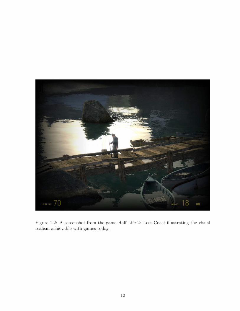
Figure 1.2: A screenshot from the game Half Life 2: Lost Coast illustrating the visualrealism achievable with games today.

12

computer-generated world. This was one of the founding stones of the area of Computer

Graphics, a large part of which aims at realistically reproducing our visual perception by

simulating matter interaction and light transport in a virtual world.4 Although the phys-

ical equations governing these phenomena are very well-known from classical physics,

performing these tasks efficiently on digital computers is extremely tough. About four

decades of research in the area of Computer Graphics has been devoted to finding suit-

able algorithms and approximations that obtain higher performance while achieving

high perceptual quality of the rendered scene. The approximations introduced are typ-

ically required to keep the computational time tractable and avoid computing detailed

features of physical reality that we are not capable of perceiving. Supplementing this

trend in ever more efficient algorithms, the computational power of desktop systems has

also increased tremendously over the last few decades. This advance has been further

accelerated by Graphics Processing Units (GPUs) designed specifically for performing

compute-intensive graphics operations in hardware. With this combination of algorith-

mic and hardware advancement, computer graphics has now matured as an area and it

is possible these days to generate scenes of stunning realism on desktop machines in-

teractively, using a combination of efficient algorithms, perceptual approximations and

fast hardware. Figure 1.2 shows a screenshot taken from the game “Half Life 2: Lost

Coast” that illustrates the realism achievable today in interactive graphics applications.

Unfortunately, work on providing an immersive aural experience, called auraliza-

tion, to complement visualization, has fallen far behind, receiving very little attention

in the interactive applications community, in comparison to Graphics. The first well-

known publication discussing the integration of sound in interactive applications was

nearly two decades ago by Takala and Hahn [100]. Their seminal work was motivated

by the observation that accurate auditory display synchronized correctly with the world

4Throughout this thesis, I use the terms “virtual world”, “game environment” and “scene” inter-changeably, unless otherwise noted.

13

displayed visually, can augment graphical rendering and enhance the realism of human-

computer interaction because in reality we use hearing and sight together, as I discussed

previously. There have also been systematic studies showing that realistic auralization

systems provide the user with an enhanced spatial sense of presence [26]. The motivation

for my thesis is to achieve this goal of producing realistic sound by mimicking reality –

use computer simulations of the physical equations governing how sounds are produced

and propagate in a scene. By grounding these simulations on the actual models of the

interacting objects and propagating the sounds in the same scene shown visually, it

is possible to design general techniques and systems that generate realistic sounds in

all possible events that might happen in an interactive application, without requiring

an artist to foresee all possible circumstances beforehand. Research work in this area

has unfortunately been sparse, although finally, the interactive applications commu-

nity is paying more attention to sound. Commercial applications, like games, reflect

the disparity between graphics and sound. Whereas some games today feature close

to photo-realistic graphics, game audio engines still rely largely on prerecorded clips

and prerecorded acoustic DSP filters, often lacking basic occlusion/obstruction effects.

The underlying technology has stayed unchanged in its essential design for nearly two

decades, despite its shortcomings. Although I discuss these in more detail in subsequent

chapters, I will mention a few of the most important deficiencies here that have guided

my work.

Most sounds we hear in games/virtual environments have no real correspondence

to the world’s physics, they are prerecorded clips played with perfect timing to give

an illusion that the graphics and sound are somehow related. This breaks down in

many instances and leads to loss of realism – we are quick to reject sounds that repeat

exactly, as artificial. After a few repetitions, we subconsciously classify them as merely

indicative rather than informative. The simple reason is that natural sounds simply

don’t behave like this, we rarely hear the exact repetition of any natural sound and we

14

respond to slight variations because they often contain useful information. For example,

consider a game scene with a cylinder rolling on the floor that is not visible to the player.

The rolling sound has a precise correlation with the roughness of the floor, material of

both the cylinder and floor, and the speed of rolling. If one uses a prerecorded rolling

clip which is insensitive to the above mentioned parameters, the user will respond to

the sound with observing subconsciously “A cylinder is rolling”, rather than “A metal

cylinder is rolling slowly on a wooden floor.” There is a lot of information contained

in this sound – The player might be able to reasonably conclude the room the other

player is in, given the wooden floor and type of cylinder. Achieving realistic audio in

movie production is comparatively easier, since only particular, known cases have to be

handled. After the visual portion of the movie is done, a foley (audio) artist can record a

highly realistic clip depending on the exact circumstances shown visually. But the very

open-ended nature of interactive applications that makes them so attractive, renders

such an approach nearly impossible, requiring huge libraries of prerecorded sounds that

cover all possibilities reasonably well – something games are forced to do today. This

process turns sound production into a huge asset creation and management problem,

while still not producing sounds that are realistic enough for a large number of cases.

In their seminal work [100], Takala and Hahn also discussed the need for adding

realistic acoustics in interactive applications. It is well-established that to give a user a

sense of presence in a scene, realistic acoustics is an indispensable requirement. Among

other things, a major challenge in this regard is the ability to model the effect of occlu-

sions and obstructions for sound. Since diffraction effects are clearly perceivable to us

in everyday life, they are added into games using hand-tuned low-pass and gain filters.

However, again, the sheer unpredictability of scenarios that will manifest in real time as

the sources and listener move, makes such an approach intractable.

15

1.2 Physically-based Simulation of Sound

The main premise behind my thesis is that if we model the wave physics underlying

acoustic phenomena at sufficient accuracy to capture the aurally relevant behavior of

the sound-producing objects and their environment using a digital computer, the result-

ing auralizations should be closely matched to our observation of reality and efficient

enough to be executed in real time. This new capability would automatically lead to a

higher level of immersion in an interactive environment, since we naturally respond to

environments using both visual and aural cues. Computer graphics has shown that this

principle can be applied to visualization by simulating light transport using physically-

based ray-optic principles and rendering the results to produce a realistic, convincing

rendition of the scene. Doing such light simulations efficiently enough for real-time

execution has been a major achievement of research in the area of computer graphics.

My thesis work is an application of this same idea for sound simulation – since

graphics in interactive applications has reached a high level of believability, to reach

the next level of immersion, a realistic rendition of both light and sound is the natural

next step. Additionally, physically-based simulation of sound seems to be the most

promising route to achieve this goal, given the open-ended nature of interactive virtual

worlds. However, as discussed earlier, sound simulation and its associated challenges

are very different in their essential character from those in graphics. Developing novel

approaches to address these challenges is the main contribution of my thesis.

Past work on using physically-based sounds has seen limited success because of two

main factors – lack of visual realism and lack of computational power. Even if the user

is presented with a highly realistic auralization, unrealistic visualizations lead to imme-

diate sensory rejection. Our visual perception and aural perception are tied together

inextricably. It is well-known, for example, that the quality and warmth of the sound in

an opera house is affected by the lighting and visual “mood” of the theater. There is no

reason the same wouldn’t apply to virtual worlds. Secondly, the computational power

16

of computers has increased tremendously in recent years, compared to ten years back

– something that has enabled many aural tasks cross the limit of interactivity. These

days, most of the computation for interactive 3D graphics is done by Graphics Processors

(GPUs). This fact, combined with the advent of high performance, multi-core CPUs,

is an important factor for the feasibility of many of the approaches I present. Also, as

I show in my work on numerical acoustics, GPUs are also very useful for providing the

raw computational power necessary for fast off-line numerical simulation, considerably

reducing the preprocessing time for acoustic simulation.

Simulating even simple sound-producing systems requires a lot of computation. As

discussed earlier, sound simulations required transient, time-domain, simulations while

resolving frequencies ranging from 20Hz to 22,000Hz, and spatial scales from millime-

ters to meters, at update rates surpassing 44,000Hz. From the practical perspective of

implementing an interactive auralization system, a central consideration is the continu-

ous nature of sound – any temporal incoherence whatsoever will be quickly and clearly

perceived. For example, any waveform discontinuity is perceived as a very audible, high

frequency “click”, which immediately degrades the audio quality dramatically. Contrast

this with visual rendering, where such jittering will only result in a decreased sense of flow

in the video. This is a very common experience: While watching a movie, we tolerate

momentary degradation in video quality quite easily but degradation in audio quality,

such as jittering, is completely unacceptable. Thus, an interactive auralization system

must provide very strict performance guarantees and should be able to adapt gracefully

to variable time constraints while performing extremely challenging computations.

Because of the computational difficulties outlined above, most real-time systems, in-

cluding the techniques I present, involve two steps: first, there is a pre-computation step

in which physical simulation or other mathematical operation, such as modal analysis, is

performed to facilitate fast computations in real time. To improve runtime performance

and memory usage, perceptual approximations are used to represent this information

17

in a compact form that can be utilized efficiently in real time. At runtime, the stored

results are used to perform interactive auralization. The main theme of my thesis is to

use well-known physical principles to model and simulate the physical aspects of sound,

and to develop and improve current computational techniques along with application

of relevant perceptual principles to enable and accelerate interactive applications with

real-time auralization.

The overall problem of sound simulation can be broken down into mainly two com-

ponents based naturally on its physics – synthesis (production) and propagation. Think

of a cup falling on the ground – after impact, its surface starts undergoing small-scale

vibrations which create pressure waves in the surrounding air. After being thus pro-

duced, these waves propagate in the scene, undergoing complex interactions with the

boundary and reaches our ears after being modified by the scene. Thus, what we hear

contains information both about the object creating the sound, as well as the scene in

which it propagates. The first part above is the problem of sound synthesis : modeling

how sound is produced by typical objects due to elastic surface vibrations upon such

events as collision and rolling. The second part is sound propagation: how the sound

thus produced propagates in an environment, as it reflects and diffracts at the scene

boundaries, before reaching the listener’s ears. My work spans both these aspects of

sound simulation, with an emphasis on efficiency and real-time execution on today’s

desktop machines. This leads me to my thesis statement.

1.3 Thesis Statement

“By exploiting analytical solutions using modal analysis to accelerate numerical simu-

lation and reducing runtime computation to capture only the perceptually important

auditory cues, one can design fast algorithms to perform real-time sound synthesis and

acoustic wave propagation on complex 3D scenes, enabling realistic, physically-based

18

auralization.”

By “realistic” in the above statement I mean sounds that, on informal listening,

at once seemed consistent with our daily experience. For my work on acoustics, com-

parisons were performed against simulations with a high-accuracy technique, for the

purpose of validation.

1.4 Challenges and Contributions

My contributions can be divided into three main areas: interactive sound synthesis, effi-

cient numerical acoustics, and interactive sound propagation. I will discuss the respective

computational challenges and my contributions in each of these areas in the following

sub-sections. Here, I describe the relationship between these different components and

how they fit in the overall goal of designing an interactive, immersive auralization frame-

work. The connection between sound synthesis and propagation is quite clear from the

perspective of an interactive application: the former deals with how sound is produced

by objects in an environment and the latter with how it propagates before reaching the

listener. It is useful to keep in mind that this classification of sound simulation into

synthesis and propagation is only pragmatic nomenclature – in reality, wave propaga-

tion underlies both of these problems: the sound of a piano string results from waves

propagating back and forth along it length and interfering, while the reverberation in a

concert hall results from waves propagating in the volume of the scene, scattering from

the walls and interfering. This similarity in physics might motivate us to think that

the same simulation technique could work for both cases. Unfortunately, this is not

the case because of the drastic differences in the computational cost for sound synthesis

and propagation for practical domains. I now describe why this is the case and give

the reader some numerical intuition of what makes sound simulation computationally

challenging.

19

Computational Cost: Recall that the speed of a sound wave in a medium, c, is

related to its frequency, ν, and wavelength, λ, by –

c = νλ (1.2)

The cost of sound simulation on a domain can be measured by its “sound-size”. Given

the diameter of a D-dimensional scene, L, and the smallest wavelength to be simulated,

λmin, the sound-size, S, of the scene is a dimensionless number defined as –

S :=

(L

λmin

)D

(1.3)

The smallest simulated wavelength, λmin, is found by considering the highest fre-

quency of interest, νmax, which yields, λmin = c/νmax. The highest frequency of interest

can be fixed based on perceptual considerations, such as the highest audible frequency

(roughly 20,000 Hz), or the highest frequency that can be simulated with feasible compu-

tational and memory costs. Intuitively, S corresponds to the number of wavelength-sized

cubes that fit in the whole domain and is the main parameter controlling the amount

of computation and memory required to do sound simulation. Stated mathematically,

after spatial discretization, the domain’s elasticity matrix is sparse with size (number of

rows/columns) proportional to S. The technique of modal analysis that was described

earlier is the most attractive option to model elastic vibrations in arbitrary domains.

This is because once modal analysis is done offline, the results can be used very effi-

ciently in real time to model any vibrations in the domain due to arbitrary excitations.

Theoretically, modal analysis applies equally well to sound synthesis and propagation,

because both are wave propagation problems and yield a corresponding elasticity matrix

on discretization. The problem is that the sound-size for sound propagation problems

is many orders of magnitude larger than synthesis problems of practical size.

For sound synthesis, L is much smaller because the dimensions of sound-producing

20

objects, such as cups, bells, boxes, musical instruments, etc. are necessarily much smaller

than the dimensions of acoustic spaces in which they are contained, such as rooms or

buildings. Additionally, sound propagates much faster in solids and liquids than in air,

which means that audible frequencies have much larger wavelengths in solids than in

air. Therefore, for sound synthesis from solids/liquids, λmin is much larger than for

propagation in air. Lastly, many sound producing objects can be treated with reduced

dimensionality. For example, the string of a piano can be treated as a 1D system, while

a drum membrane can be modeled very well as a 2D system. In fact, most thin-shell

objects can be approximated as 2D vibrational systems with good accuracy. Sound

propagation, on the other hand, almost invariably requires a 3D treatment. Here’s a

quick numerical comparison of the sound-size of a solid steel box (c ≈ 3000m/s for shear

waves) versus a concert hall (c ≈ 340m/s for sound in air), with νmax = 20, 000Hz for

both cases:

L = 1.0m, λmin = 0.15m, D = 3 =⇒ Sbox ≈ 300

L = 20m, λmin = 0.017m, D = 3 =⇒ Shall ≈ 1, 600, 000, 000 (1.4)

Thus, the sound-size, S, for sound propagation is many orders of magnitude larger

(million times in the above example) than sound synthesis. The computational cost and

memory requirements of modal analysis scale as S3 and S2 respectively. It must be clear

in context of the above examples why modal analysis works quite well for the purpose

of sound synthesis, but is completely infeasible for acoustics on realistically large 3D

scenes. On desktop machines today, modal analysis can be performed for S in the range

of few thousand while consuming less than 4 GB of memory and taking a few hours

of computation time, thus allowing modal analysis for most sound-producing objects.

As for propagation, taking the above example, performing a full modal analysis on the

orchestra hall would take 1018 times the computation time as the steel box and 1012

21

times the memory. Clearly, a different kind of decomposition of computation into offline

and real-time components has to be explored, which is one of the contributions of my

dissertation research on interactive sound propagation.

In the first part of my thesis on interactive sound synthesis, modal analysis is used

for precomputation as it can be feasibly performed for typical sound-producing objects

while staying within the constraints of a few GB of main memory and a few hours of

computation. Therefore, in this part of my dissertation, performing the precomputation

was not the main challenge and I focused directly on the issues with handling lots of

sounding objects in real time. Existing techniques could only handle a few (roughly

ten) objects and my key contribution was in designing an perceptual approximations

and interactive techniques for handling hundreds of objects in real time while ensuring

smooth degradation in perceived quality, as available computation fluctuates in a typical

real-time interactive application.

In the second part of my dissertation, I have developed a fast, time-domain numerical

acoustic simulation technique. For time-domain acoustic simulation, the current state

of the art in room acoustics, as well as in computational acoustics to a large extent, is

the Finite Difference Time Domain (FDTD) technique. FDTD is enormously more effi-

cient than modal analysis for performing simulations in the kilohertz range on large 3D

scenes and satisfies all the criteria for sound simulation that I discussed earlier, namely,

time-domain, broadband simulations that capture all wave properties. Unfortunately,

the computational time and memory requirements of accurate, high-order FDTD, even

though far superior to modal analysis, were still insufficient for my purpose, even for

moderate-sized 3D scenes. Thus, a major portion of my work is devoted to developing a

numerical acoustics simulator that exploits suitable physical approximations consistent

with room acoustics (mainly that the speed of sound is constant in the domain), to make

simulations on acoustically large environments feasible on a desktop computer. I was

able to successfully develop such a simulator, that uses an adaptive rectangular decom-

22

position (ARD) of the scene. The ARD simulator is capable of performing simulations

that used to take days with a reference, high-order FDTD, in minutes on a desktop

computer.

In the third part of my dissertation on interactive sound propagation, I have used

my ARD simulator to perform acoustic precomputation and enable realistic, interactive,

acoustics for moving sources and listener, thus “closing the loop,” yielding a system that

generates auralizations using wave-based acoustics simulation in real time. Numerical

simulations using ARD are utilized to precompute acoustic responses for different source

locations in an environment at a dense sampling of listener locations. These results are

then stored in a compact representation that allows for very efficient storage and usage

at runtime, among other benefits. Thus, it becomes possible to design an interactive

system that uses numerical acoustics in real time to perform auralizations that include

the effects of physically complex and perceptually important phenomena such as diffuse

reflections, reverberation, focusing and occlusion/obstructions.

In totality, these three parts of my dissertation form a solution to the overall prob-

lem of interactive physically-based sound simulation. My work contains contributions in

both the important aspects of this overall problem, namely, synthesis and propagation.

In the following, I separately discuss in technical detail, the specific challenges and my

contributions in these three portions of my thesis. There remain many challenges and

interesting problems to be addressed in this area that are being addressed in concur-

rent work, as well as problems that I intend to investigate in the future. This thesis

offers a substantial step forward in the design of a comprehensive and consistent set of

techniques for performing interactive and immersive physically-based auralization. In

future interactive applications, one can imagine the sound being produced as well as

propagated in the scene directly from the geometry and material properties of the world

and objects contained in it, leading to rich, realistic games and virtual worlds.

23

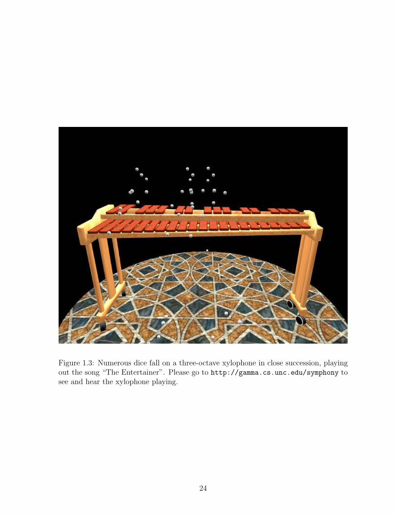
Figure 1.3: Numerous dice fall on a three-octave xylophone in close succession, playingout the song “The Entertainer”. Please go to http://gamma.cs.unc.edu/symphony tosee and hear the xylophone playing.

24

1.4.1 Interactive Sound Synthesis

As noted earlier, most interactive applications today employ recorded sound clips for

providing sounds corresponding to object interactions in a scene. Although this ap-

proach has the advantage that the sounds are realistic and the sound-generation process

is quite fast, there are many physical effects which cannot be captured by such a tech-

nique. Once such example of a rolling cylinder was given earlier. More generally, in a

typical collision between two objects, the loudness and timbre of the sound is determined

by the magnitude and location of the impact forces – a plate sounds very differently when

struck on the edge compared to when it is struck in the middle. Consequently, if the

collision scenario changes slightly, the sound exhibits a corresponding change. Such

subtle effects can add substantial realism to a typical scene by avoiding the repetitive-

ness common to recorded sound clips. However, developing a system which produces

sound using physically-based principles in real time poses substantial difficulties. The

foremost requirement is the presence of an efficient dynamics engine which informs the

sound system of object collisions and the forces involved. Fortunately, many present-day

games easily meet this requirement, with physics engines such as NVIDIA PhysX [3] and

Havok [2]. Open-source dynamics engines, such as ODE [4], are also available. Given

a dynamics simulator, the essential challenge then is to synthesize the sound efficiently

enough to play in real time while taking only a small portion of the total running time,

which is usually dominated by graphics and rigid-body simulation. As of today, sound

engines can typically only afford a few hundred CPU cycles per object per sound sample

for many interactive applications.

In this part of my thesis, I present an approach that meets the interactive perfor-

mance requirements outlined above, while ensuring high realism and fidelity of the sound

produced. Given an object’s geometry and a few material parameters, a spring-mass

model approximating the object’s surface is constructed. I show that although a spring-

mass system is a coarser approximation than FEM models used in prior approaches

25

[17, 63, 64], it is an adequate model to capture the small-scale surface vibrations that

lead to the generation of sound in nature. The advantage of using spring-mass systems

is the ease of implementation and ability to easily handle surface meshes designed for

visual display. I show how this formulation yields an analytical solution to the equation

of motion for the surface of the object which can then be used to find the resonant modes

of the object surface using modal analysis. The runtime computation consists of calcu-

lating each mode’s contribution which is then suitably mixed to produce the objects’

sound. Modeling only the surface works well for thin-shell objects. For solid objects, it

is possible to form spring-mass models of the whole volume, at higher precomputation

cost, without changing any other details of the technique I present.

However, a naive implementation of such an approach requires a very high number

of modes to be mixed per object and consequently, only a few (less than ten) sounding

objects in real time can be handled by prior techniques. I present several perceptually-

motivated acceleration techniques to reduce the number of modes being mixed while

ensuring minimal perceptual degradation. In addition, the sound quality and the as-

sociated computational cost for each object is scaled dynamically in a priority-based

scheme which guarantees that the total sound production meets stringent time con-

straints, while preserving the overall aural experience as far as possible. My approach

has the following features –

• It is based on a discretized physically-based representation that offers simplicity

of formulation and ease of implementation;

• It makes no assumptions about the input mesh topology – surface meshes used for

physics can be used directly for sound synthesis;

• It is capable of yielding both impact and rolling sounds naturally, without any

special-case treatment;

• It uses perceptually-motivated approximations enabling rich environments con-

26

sisting of hundreds of sounding objects, with insignificant reduction in the overall

audio quality.

• Its easy to integrate with commonly available physics engines.

To the best of my knowledge, with the possible exception of methods that rely on

physical measurements, no work prior to the publication of my work in [71, 72, 70] has

been demonstrated to handle complex scenarios (e.g. see Figs. 1.3 and 3.6) in real time.

There has been more recent work improving on these techniques, I discuss those in the

next section.

1.4.2 Efficient Numerical Acoustics

As explained earlier, the complimentary problem to sound synthesis is that of simulat-

ing sound propagation in arbitrary spaces. In this part of my thesis, I have addressed

the problem of numerical simulation of acoustic wave propagation, also referred to as

computational acoustics. As I discussed previously, due to the physical properties of

sound, a fully wave-based, time-domain, broadband simulator is required. Numerical

approaches for sound propagation attempt to directly solve the acoustic wave equation,

that governs all linear sound propagation phenomena, and are thus capable of perform-

ing a full transient solution that correctly accounts for all wave phenomena, including

diffraction, elegantly in one framework. Since I use a numerical approach, my imple-

mentation inherits all these advantages. This characteristic is also the chief benefit my

method offers over geometric techniques, which I will discuss in detail in Chapter 4.

For the purpose of my thesis work, the eventual application for this simulator is

real-time auralization, which is discussed in detail in the next sub-section. However, the

ideas provided here would be applicable to many other wave propagation problems as

well, for example, in electromagnetic wave propagation. The key assumptions underlying

my approach are – firstly, the wave propagation is governed by linear equations which

27

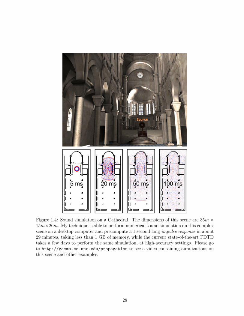
Figure 1.4: Sound simulation on a Cathedral. The dimensions of this scene are 35m×15m×26m. My technique is able to perform numerical sound simulation on this complexscene on a desktop computer and precompute a 1 second long impulse response in about29 minutes, taking less than 1 GB of memory, while the current state-of-the-art FDTDtakes a few days to perform the same simulation, at high-accuracy settings. Please goto http://gamma.cs.unc.edu/propagation to see a video containing auralizations onthis scene and other examples.

28

allows the principle of superposition to be used. Secondly, the speed of wave propagation

should be piece-wise constant over the domain of interest. My technique can be applied

as long as these two assumptions hold, to yield speeds much faster than is achievable

with standard techniques that make more general assumptions.

The input to an acoustic simulator is the geometry of the scene, along with the

reflective properties of different parts of the boundary (boundary conditions) and the

locations of the sound sources and listener. The final goal in my case is to auralize

the source sound – predict the sound the listener would hear. Recall that this process

involves complex physical interactions such diffraction (sound bending around obstruc-

tions), reflecting and scattering from the scene geometry, etc. All these interactions are

captured succinctly by computing an impulse response (IR) of the scene under consider-

ation that captures its complete response in time for a given source and listener location.

Intuitively, the impulse response is the sound received at the listener if an ideal Dirac

delta impulse is played at the source. Note that the impulse response varies, depending

on both the source and listener locations.

Computational acoustics has a very diverse range of applications, from noise control

and underwater acoustics to architectural acoustics and acoustics for virtual environ-

ments (VEs) and games. For a general introduction to the whole area of acoustics, I

refer to the text by Kinsler [47]. Although each application area has its own unique

requirements for the simulation technique, all applications require some level of physical

accuracy, although with different error tolerances. For noise control, accuracy translates

directly into the loudness of the perceived noise. For architectural acoustics, accuracy

has implications on predicting how much an orchestra theater enhances (or degrades)

the quality of music. For interactive applications like VEs and games, physical accuracy

directly affects the perceived realism and immersion of the scene. This is because we are

used to observing many physical wave effects, such as diffraction, in reality and their

presence in the scene helps to convince us that the computer-generated environment is

29

realistic.

For most acoustic simulation techniques, the process of auralization can be broken

down into two parts: (a) preprocessing; and (b) sound rendering. During preprocessing,

an acoustic simulator does computations on the environment to estimate its acousti-

cal response at different points. These are encoded as impulse responses. The exact

precomputation depends on the specific approach being used. For my approach, the

preprocessing consists of running a simulation from a source location, which yields the

impulse responses on the whole simulation grid in the scene in one simulation. The

simulation grid is typically quite fine, with a resolution of around 12 cm for a 1kHz

band-limited simulation. The rendering at runtime can then be performed by convolv-

ing the source signal with the calculated impulse response at the listener’s location. This

part of my dissertation deals with the preprocessing phase of acoustic prediction that

computes impulse responses. The subsequent real-time auralization is the focus of the

next part of my thesis on interactive sound propagation.

I present a novel and fast numerical approach that enables efficient and accurate

acoustic simulations on large scenes on a desktop system in minutes, which would have

otherwise taken many days of computation on a small cluster. An example of such

a scene is the Sibenik cathedral shown in Figure 1.4. This scene would have taken a

few days for a 1 second long simulation on a small cluster (due to memory limitations)

with the current state-of-the-art in room acoustics, the Finite Difference Time Domain

(FDTD) method. With my technique, this same simulation can be completed in about

30 minutes on a desktop computer equipped with a NVIDIA GTX280 GPU.

Most interactive applications today, such as games, use artificial reverberation filters

(or equivalently, impulse responses) that are not based on the environment. Instead,

they roughly correspond to generic acoustical spaces with different sizes – “Large hall”,

“narrow corridor” etc. [5] The filters are assigned to different parts of the world to

capture the realism and mood of the scene, and are typically assigned by experience

30

game audio designers who also have a good intuition of how the artificial reverberator

works and what all of its parameters do. In reality, the acoustics of a space exhibits

perceptibly large variations depending on its geometry, wall material, and other factors

[51]. There is not even a guarantee that the artificial reverberator’s controls provide

enough expressiveness to capture all these factors.

A possible alternative to obtain realistic filters for interactive auralization would

be to do actual measurements on a scene instead of performing a simulation. This is

analogous to using recorded clips instead of synthesizing sounds. Not only is it difficult

and time-consuming to do this for real scenes, but for virtual environments and games,

one would need to physically construct scale physical prototypes because the scenes

don’t exist at all in reality! This is of course, prohibitively expensive, cumbersome

and impractical. What if the game artist decides to change the game map to improve

gameplay by partially removing a wall? One would need to re-build the scale model

and re-measure everything. This is even more impractical considering that most games

today encourage users to author their own scenes. Given all these factors, especially the

last one, simulation is clearly the best approach since the automatically generated filters

would be realistic and correspond to the scene presented visually. If artistic control is

desired, these filters could then be modified by an artist. This is not the complete story,

as far as games go – one also needs a way to efficiently apply these filters to sounds in

real time, and for that a fast and memory-efficient sound rendering system is required,

the topic of the next part of my work.

Thus, numerical approaches offer the attractive option to take the scene geome-

try and automatically provide realistic and immersive acoustics in games and virtual

environments which account for all perceptually-important auditory effects, including

diffraction. However, this realism comes at a very high computational cost and large

memory requirements. In this part of my thesis, I have developed a highly accelerated

numerical technique that works on a desktop system and can be used to precompute

31

high-quality impulse responses for arbitrary scenes without any human intervention.

Another application of this simulator that I have not explored in depth in my work,

is in the traditional application of sound simulation to determine the acoustic quality

of concert halls. Since my simulator solves for the complete sound field in a scene,

an acoustic consultant could give as input the CAD geometry of the hall and actually

visualize how the sound wavefronts propagate in the scene over time. This would help

him/her make guided decisions about what changes need to be made to the scene to

counter any perceived acoustic deficiencies. For example, to identify the portion of a

wall that is causing an annoying, strong reflection. Refer to the bottom of Figure 1.4

for an example of such a time-stepped field visualization.

Main Results: My technique takes at least an order of magnitude less memory and

two orders of magnitude less computation compared to a standard numerical implemen-

tation, while achieving competitive accuracy at the same time. It relies on an adaptive

rectangular decomposition (ARD) of the free space of the scene. This approach has many

advantages:

1. The analytical solution to the wave equation within a rectangular domain is known.

This property enables high numerical accuracy, even on grids approaching the

Nyquist limit, that are much coarser than those required by most numerical tech-

niques. Exploiting these analytical solutions is one of the key reasons for such a

drastic reduction in computation and memory requirements. The main reason such

solutions can be employed is the assumption that the speed of sound is constant

in the domain, which holds quite well for the purpose of auralization.

2. Owing to the rectangular shape of the domain partitions, the solution in their

interior can be expressed in terms of the Discrete Cosine Transform (DCT). It is

well-known that DCTs can be efficiently calculated through an FFT. I use a fast

implementation of FFT on the GPU [36], that effectively maps the FFT to the

32

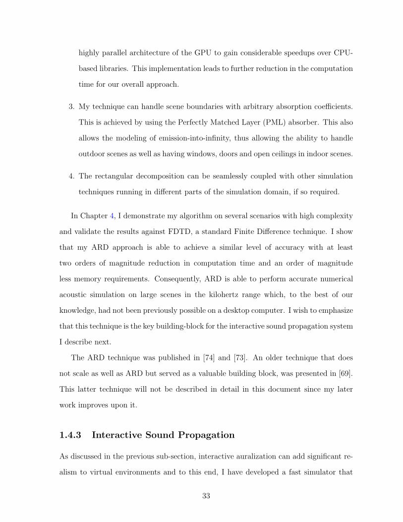
highly parallel architecture of the GPU to gain considerable speedups over CPU-

based libraries. This implementation leads to further reduction in the computation

time for our overall approach.

3. My technique can handle scene boundaries with arbitrary absorption coefficients.

This is achieved by using the Perfectly Matched Layer (PML) absorber. This also

allows the modeling of emission-into-infinity, thus allowing the ability to handle

outdoor scenes as well as having windows, doors and open ceilings in indoor scenes.

4. The rectangular decomposition can be seamlessly coupled with other simulation

techniques running in different parts of the simulation domain, if so required.

In Chapter 4, I demonstrate my algorithm on several scenarios with high complexity

and validate the results against FDTD, a standard Finite Difference technique. I show

that my ARD approach is able to achieve a similar level of accuracy with at least

two orders of magnitude reduction in computation time and an order of magnitude

less memory requirements. Consequently, ARD is able to perform accurate numerical

acoustic simulation on large scenes in the kilohertz range which, to the best of our

knowledge, had not been previously possible on a desktop computer. I wish to emphasize

that this technique is the key building-block for the interactive sound propagation system

I describe next.

The ARD technique was published in [74] and [73]. An older technique that does

not scale as well as ARD but served as a valuable building block, was presented in [69].

This latter technique will not be described in detail in this document since my later

work improves upon it.

1.4.3 Interactive Sound Propagation

As discussed in the previous sub-section, interactive auralization can add significant re-

alism to virtual environments and to this end, I have developed a fast simulator that

33

Figure 1.5: Train station scene from Valve’s SourceTM game engine SDK (http://source.valvesoftware.com). My method performs real-time auralization of soundsfrom dynamic agents, objects and the player interacting in the scene, while accountingfor perceptually important effects such as diffraction, low-pass filtering and reverbera-tion. Please go to http://gamma.cs.unc.edu/PrecompWaveSim to see a video contain-ing auralizations on this scene and other examples.

34

allows quick precomputation of acoustic impulse responses using wave propagation. Per-

ceptually realistic simulation of sound propagation must capture two interrelated wave

effects: diffraction and scattering since they result in many gross acoustic effects ob-

served in daily life. Smooth reduction in volume as one walks through a doorway or

behind a building is due to high-order diffraction. Smooth loudness variation in the

sound field of a furnished room results from diffracted scattering off its complex geome-

try. Neglecting diffraction leads to clicking artifacts and incoherent loudness fluctuation,

as well as unnatural termination of sound before it reaches occluded regions.

The input to an interactive sound propagation system is the scene geometry as well

as the locations of multiple sources, the sounds they are playing and the location and

orientation of the listener. The source sounds may be pre-recorded or synthesized using

the techniques I’ve described earlier. The objective is to auralize the final sound at the

listener, assuming the sources as well as the listener may move about. Performing such

auralization while capturing all the acoustic effects in real time within a complex 3D en-

vironment presents a challenging problem for current approaches. By “complex”, I mean

“containing acoustically relevant scene features at length scales down to centimeters”

(see Figure 5.4a). Sound frequencies up to 5 kHz scatter diffusely from “rough” surface

features at centimeter scales and are mostly unresponsive to finer detail while higher fre-

quencies are more strongly absorbed as they travel through air or scatter off surfaces [51,

p. 27]. My method is limited to static scene geometry. Fortunately, the static portion

of most spaces largely determines the overall acoustics of common architectural/virtual

spaces, thus covering a large set of applications. For example, the overall acoustics of

a concert hall is not affected drastically by opening or closing a door. Moreover, the

local effects of moving geometry could be used to augment the simulation performed

on the static portion of the scene in the future. Continuing the previous example, any

outside noise entering through the opened door could be added-in at run-time using fast

approximations to augment the total sound field.

35

Existing methods to solve this problem are geometric, and trace rays or beams from

the source into the scene to collect their contributions near the listener. These methods

have the advantage of handling dynamic scenes, but at the cost of high computational

requirements at runtime, consuming 8 cores to auralize a single moving source [18]. Most

current applications do not invest such computational resources on audio. In contrast,

my approach has been explicitly designed to consume a single core while allowing tens of

moving sources. In addition, there are many disadvantages of geometric approximations

that my work aims to alleviate. Methods based on conservative beam tracing split the

beam when it encounters geometric discontinuities, leading to slow performance in com-

plex scenes and exponential scaling in the reflection order [33, 18]. A related problem

arises for ray-tracing methods, which must sample a huge number of rays to capture

multiple-bounce propagation and avoid missed contributions. In practice, meshes must

be simplified and detailed interior objects replaced by simpler proxies to achieve interac-

tive performance, substantially increasing manual effort for producing acoustic geometry.

Automatic methods to do this are a nascent area of research [94]. Handling diffraction

with geometric approaches is challenging, especially for complex scenes [15]. At long

sound wavelengths, current geometric edge-diffraction models either ignore global effects

from complex geometry or require too much computation to run interactively.

Even though I have designed a substantially faster acoustics solver than the state of

the art, it is still at least 3 orders of magnitude too slow for on-the-fly evaluation. In

order to enable real-time wave-based acoustics, my solution is to pre-compute an off-line,

wave-based simulation for a given static environment in terms of its 7D spatially-varying

acoustic impulse response (IR), S(t, ps, pr), where t is time, ps is source position, and

pr is receiver position. That is, for each possible pair of source and listener locations in

3D, a time-series is stored, which is the impulse response at the listener from the source

location. This can be reduced to a 6D problem by restricting the listener to a 2D plane

in the scene and leveraging acoustic reciprocity which dictates that the impulse response

36

stays invariant if the source and listener locations are swapped with each other. This

dimensionality reduction leads to nearly 10 times reduction in both the runtime memory

requirement, as well as the pre-processing time. Even so, the computational and storage

requirements are huge. With my ARD technique, simulating a one-second response at

a single source position in a scene of volume 123m3 bandlimited to frequencies up to

1kHz requires 30 minutes of computation and generates 24GB of data for a single source

location. Simulating over many different source locations quickly becomes intractable.

To give the reader a more concrete intuition of the memory and computational

requirements of a brute-force approach, lets consider a typical scene with size 12m x 12m

x 12m. Additionally, lets assume the length of the required IR to be about 1 second.

Assuming a band-limited simulation till 1 kHz, the corresponding grid cell-size is about

12 cm, with an update rate of 6000 Hz. My simulator typically takes about 150 ms (milli-

second) per step for a scene with this air volume. Thus, every 1 second long simulation

takes 6000 × 0.15 = 900 seconds, which is 15 minutes. Now consider the complete 7D

space mentioned above, with no sub-sampling and no dimensionality reduction through

acoustic reciprocity. The space requirement is about – 106 × 106 × 6000 × 4 bytes =

24 petabytes and the corresponding pre-processing time is – 106 × 15min = 28 years!

This is obviously completely impractical. By sub-sampling at about 1 meter resolution

these numbers are reduced drastically to about 91 gigabytes and 20 days respectively.

Using acoustic reciprocity to reduce dimensionality leads to a further reduction to 11

gigabytes and 2 days respectively. Using the techniques I describe next, these numbers

can be reduced further to a few hundred megabytes and 2-3 hours respectively.

My technique exploits human auditory perception using the well-known ER/LR per-

ceptual model [51, p. 98]. This model temporally decomposes sound propagation in a

typical acoustic space into two parts. The first part is the early reflections (ER) phase

containing sparse, high-energy contributions corresponding to the direct sound and ini-

tial reflection/diffraction contributions which are processed separately in the human

37

brain to some degree. As time progresses, the response smoothly transitions into the

second part – the late reverberation (LR) phase representing the later arrival of many,

nearly simultaneous wavefronts which the human brain fuses and is mainly able to only

infer the statistical properties of the sound decay. While the ER exhibits significant

perceptual variation within an environment depending on the source and listener loca-

tion, the LR can be approximated as a property of the room itself, since its statistics

don’t vary much within a room. Perceptually, the ER conveys a sense of location, for

example, occlusion information, while the LR gives a global sense of the scene – its size,

level of furnishing and overall absorptivity. For example, in a concert hall, different seats

typically have different sound quality because of variation in the ER. However, every

concert hall still has a clearly identifiable, “acoustic identity”, which is captured by its

LR, which stays largely invariant perceptually over different seats in the hall. Current

techniques used in games using artificial reverberation techniques capture the LR, but

completely fail to a large degree in capturing the spatial variation in the ER.

The LR is extracted in my technique by performing a 1-2 second simulation from

a source placed at the room’s centroid and analyzing its impulse response (IR) at a

receiver in the same place. This result determines the time length of the ER, as well as

the per-room LR filter called the late reverberation impulse response (LRIR). ER length

is 50-200ms for rooms of typical size. Simulations are then run with the source placed

at all sample points on the 2.5D grid described above. For each source position, the

resulting early reflections impulse responses (ERIRs) are recorded at sample points over

the scene’s 3D volume. This two-step approach reduces the time duration of expensive

ER simulations from 1-2s to 50-100ms, saving at least 10× in precomputation time and

runtime storage.

The ERIRs recorded for each source-listener pair are then extracted and compactly

encoded using a novel, perceptually-based technique. ERIRs contain distinct pressure

peaks in time, corresponding to wavefronts arriving at the listener. My technique then

38

extracts the highest-energy peaks (yielding roughly 30-40 in most cases) and stores their

delay and attenuation in the time domain. Peak data is wide-band information that

captures reverberation and interference but ignores diffraction low-pass filtering, so I add

a residual frequency trend representation which restores these effects and allows them

to be plausibly extrapolated to frequencies beyond the ones simulated. Compared to

direct storage of simulated ERIRs, this reduces memory use by 10 times while encoding

all-frequency information.

A novel run-time system propagates source sounds based on this precomputed data.

Spatial interpolation of IRs is required as sources and listener move since these positions

are subsampled in my system to about 1m. Straightforward waveform interpolation

yields erroneous timbral coloration and “gurgling” artifacts; my technique interpolates

in the encoded space of peak times and amplitudes instead, to avoid such artifacts.

The ERIR is then spatialized to the listener’s left and right ears, the LRIR added, and

the source sound convolved in the frequency domain with the final computed impulse

responses for each ear.

My thesis is the first to achieve real-time, wave-based sound propagation, including

high-order, frequency-dependent sound scattering and diffraction, for moving sources

and listener in environments of the complexity and size I demonstrate. I propose a

novel decomposition of the computation into three parts: an off-line wave-based simula-

tion on the static scene (which is performed using the ARD technique I have developed),

an off-line perceptually-based encoding of the resulting IRs, and a run-time engine. My

technique automatically computes from simulation both the ER and LR and separates

them based on echo density. My new IR encoding extracts peaks and a residual fre-

quency trend. My key contributions include – (1) computing this information from the

bandlimited results of numerical simulation, (2) extrapolating it to higher frequencies

in a perceptually plausible manner, (3) employing a grid-based sampling for moving

sources and listener along, and (4) using one which exploits acoustic reciprocity. By

39

using reciprocity, handling ER and LR separately and expressing the ER compactly, I

obtain runtime memory usage reduction of 1000 times. This number is even larger if one

considers sub-sampling is space. The run-time system then efficiently decodes, interpo-

lates, and convolves source sounds with these encoded IRs in the frequency domain,

supporting tens of moving sources and a moving listener in real time.

Main Contributions: My work is the first to achieve real-time, wave-based sound

propagation of moving sources and receivers in complex indoor and outdoor environ-

ments. The main features of my technique are –

• A novel decomposition of the computation into three parts: an off-line wave-

based simulation in the static scene, an off-line perceptually-based encoding of the

resulting IRs, and a run-time auralization engine.

• Effective use of Acoustic Reciprocity to reduce runtime memory usage and pre-

processing time by a factor of ten;

• Automatically compute both the ER and LR from simulation and separate them

based on echo density;

• Representation for Impulse Responses based on ER/LR model, reducing runtime

memory usage and pre-processing time further by ten times;

• My new IR encoding extracts peaks and a residual frequency trend yielding a

further 10 times reduction in memory usage. Computing this information from

the bandlimited results of numerical simulation, extrapolating it in a perceptually

plausible manner and employing a grid-based sampling for moving sources and

listener are all novel contributions.

• A novel runtime technique for fast interpolation of sampled Early Reflection IRs

that preserves important perceptual properties; and

40

• The first real-time auralization system that captures wave-based effects such as

realistic occlusion/obstuction in complex, static indoor and outdoor scenes with

tens of moving sound sources and listeners on a desktop computer.

The technique presented in this part of my thesis was published in [75].

1.5 Thesis Organization

The following chapters are organized as follows. In the next chapter, I discuss related

work in the areas of sound synthesis and sound propagation. The three subsequent

chapters correspond to the three main parts of my thesis work in the same order as

discussed here: interactive sound synthesis, efficient numerical acoustics, and interactive

sound propagation. I conclude my thesis with a summary of the main contributions, as

well as a discussion of future work.

41

Chapter 2

Previous Work

In the most general case, sound can be defined as elastic waves propagating in a physical

medium. One way to organize all applications of sound is based on the phase of the

medium of propagation, as there are important physical differences in wave propagation

depending on whether the phase of the medium is solid, liquid or gas. In the area of

structural and vibrational engineering, one is mainly concerned with solid media and

the dynamic behavior of different structures, such as bridges, under time-varying loads.

Such problems constitute the area of structural or vibrational engineering. On a smaller

scale, the same governing equations also describe a cup’s surface vibration upon being

hit, or a piano string’s vibration after being struck by the hammer, which is related to

the problem of interactive sound synthesis. The medium of sound propagation could

be liquid, such as water, which is the area of underwater acoustics having wide-ranging

applications, such as sonar sensing to image the ocean floor. The medium could be

gaseous, such as air, in which case we are concerned with acoustic wave propagation

with applications ranging from noise control in an air-plane’s cabin to concert hall

design. My work on interactive sound propagation is closer in its motivation to the

latter application.

One might question in light of the above discussion why there is any need for re-

search on sound simulation in the context of interactive applications, which is the focus

of my thesis, since the governing physical equations are the same as the engineering ap-

plications outlined above. Further, computer simulation techniques developed in these

engineering disciplines, as well as techniques for modeling wave propagation in related

areas, such as electromagnetic simulation, have clear and direct applications to inter-

active sound synthesis and propagation. But, there are two crucial differences from

engineering problems when performing sound simulation for interactive applications –

1. Real-time, memory-efficient execution: Interactive applications require that

the results of sound simulation be presented in real time. Due to this requirement,

the practical limitations of today’s desktop computation power require the com-

putations to be split into precomputation and runtime execution phases, for most

cases. The runtime computation should execute in real time and it should also

have a small memory footprint. This means that if precomputation is required,

it should generate appropriate, compact results that capture all the “necessary”

features of the simulated sound. What I mean by necessary is discussed below in

the next point. These requirements are made even more stringent because in most

interactive applications, there are other components besides audio as well, which

typically leave only a small fraction of the available computation power for audio.

2. Exploiting auditory perception: The high computation and memory efficiency

requirements mentioned above can be met by keeping in mind that very high nu-

merical accuracy is not always a necessary requirement for interactive applications,

since the end-consumer is the human auditory system. This aspect can be exploited

by avoiding computation of inaudible features of the sound, and/or removing them

during the precomputation phase to reduce the memory footprint.

Besides these two differences, from a pragmatic point of view, it is desirable for

interactive applications that the precomputation time also be reasonable, in the range

of a few hours on a desktop computer. A few minutes would be even more desirable, so

43

that, for example, a game artist could iteratively try out different scenarios.

Thus, since most engineering techniques are not designed for on-the-fly evaluation,

interactive sound simulation presents unique challenges. Additionally, because one can

exploit human auditory perception, this immediately opens up many possibilities for

acceleration techniques in this area. One might further argue that a few decades of

improvement in hardware is going to allow direct application of robust solvers used in

engineering applications in real time, making such developments obsolete. The counter-

argument is that techniques developed especially for interactive applications that are

faster today will be faster tomorrow. This means that a decade from now, much more

could be performed in real-time than today – hardware improvements will improve the

performance of both kinds of algorithms by similar amounts. Further, it might well turn

out that while exploring numerical and perceptual approximations, one comes across

useful improvements that apply to some engineering applications as well. I have come

up with one such example in my own research described here – The fast wave simulator

I have developed (ARD), will be directly applicable to traditional room acoustics appli-

cations after adding a few features, most notably, frequency-dependent absorption, and

might serve as a valuable room acoustic prediction tool. ARD might even be applicable

to electromagnetic scattering, if the interface errors can be reduced from the current -40

dB to -80 dB (which is close to what current FDTD techniques can achieve in this area

[99]). This may be achieved by using interface operators that have an order of accuracy

higher than six, as employed currently. Additionally, one might explore compact stencils

optimized for lowering the frequency-response of the artificial interface. Since ARD is

roughly 100 times faster than a high-order FDTD, slowing ARD down by a small factor

for achieving this additional accuracy gain will be worthwhile.

My discussion of previous work falls into two parts, both in the context of interactive

applications. In the first part, I discuss previous techniques for sound synthesis, focus-

ing on generating sounds from solid objects in real-time. The second part presents a

44

discussion of simulation methods proposed in the literature for modeling acoustic wave

propagation in room acoustic applications and discusses my work on developing a fast

numerical acoustics simulator (ARD) in this context. Lastly, I contrast interactive au-

ralization techniques and their room acoustic simulation counterparts with my work on

using ARD for interactive auralizations with related work in this area. Most of the work

discussed here is based on geometric techniques because there has been very limited

work on wave-based simulation for interactive auralization.

2.1 Interactive Sound Synthesis

The following discussion will focus on sound synthesis based on physical deformation

modeling of underlying systems. There is a rich history of real-time sound synthe-

sis based on what Perry Cook calls “physically-inspired” sound modeling where the

emphasis is on capturing, in simple parametric models, the essential sound-producing

mechanism behind any natural sound-producing phenomenon. This is in contrast to my

overall “physically-based” approach here which consists of simulating the objects’ actual

surface deformation over time. For a great introduction to physically-inspired real-time

techniques, as well as a brief discussion of physically-based techniques, the reader is

refereed to Cook’s book on the subject [21]. A very useful online resource on signal

processing for sound synthesis and digital waveguides for musical synthesis is Julius O.

Smith’s book available freely online [95].

The concept of modeling the surface vibrations of objects using discretized physical

models in real time for generating sounds was first proposed by Florens and Cadoz [30],

who used a system of masses and damped springs to model 3D shapes and developed

the CORDIS-ANIMA system for physically-based sound synthesis. More recently, nu-

merical integration with a finite element approach was proposed as a more accurate

technique for modeling vibrations [17, 63]. These methods had the advantage that the

45

simulation parameters corresponded directly to physically measurable quantities and

the results were more accurate. The main issues were the complexity of formulation and

implementation and the low speed of the resulting simulation.

To remedy the performance issue of the above methods, van den Doel and Pai [109,

110] suggested using the analytically computed vibrational modes of an object, instead

of numerical integration, leading to considerable speedups and enabling real-time sound

synthesis. But, since the solution of PDEs governing the vibration of arbitrary shapes

are very complicated, the proposed system could only handle simple systems, such as

rectangular or circular plates, for which analytical solutions are known. To handle more

complex systems which do not admit direct analytical solution, two approaches have

been proposed in literature. The first approach, [113] used physical measurements on a

given shape to determine its resonant vibration modes and their dependence on the point

of impact. Later, these modes may be appropriately mixed in a real-time application

to generate realistic synthetic sounds. But, arbitrary 3D models have to be physically

obtained or constructed in order to find their aural properties, which can a serious

limitation in many cases. For example, when the object is created entirely virtually, as

is done for computer games. In [64], O’Brien et al. addressed this problem and proposed

a method for handling arbitrarily-shaped objects by discretizing them into tetrahedral

volume elements. They showed that the corresponding finite element equations can be

solved analytically after suitable approximations using modal analysis. Consequently,

they were able to model arbitrarily shaped objects and simulate realistic sounds for a

few objects at interactive rates.

My work shares some common themes with [64]. Their work used an FEM-based

model for the elastic behavior of the object. I propose a simpler system of point-masses

and damped springs for modeling the surface vibrations of the object and it also submits

to an analytical solution in a similar fashion, while offering much greater simplicity of

formulation and ease of implementation. The complexity of scenes demonstrated in [64]

46

is low, containing less than 10 sounding objects and the interactions captured are mainly

due to impacts. My main contribution is a method that scales to handling hundreds

of objects in real time using psychoacoustic principles. Also, it is capable of producing

realistic rolling sounds in addition to impacts.

The main bottleneck at runtime in all techniques that utilize modal analysis is eval-

uating and mixing all the resonant modes of the object at runtime. Most approaches,

including mine, use a time-domain approach for evaluating the modes since they cap-

ture the initial transient of an impact sound quite well. There has been very recent

work exploring the possibility of evaluating and mixing the modes in frequency-domain

instead [11] to obtain significant performance gains, although at some expense in quality

for capturing the transients right after impact.

Often, immersive environments are both visually and aurally complex. The problem

of scheduling multiple objects for sound synthesis has been addressed before in [31]. They

exploited a model of imprecise computation in [20], and proposed a system in which the

objects are iteratively assigned time quotas depending on the availability of resources

and priorities of the objects. My approach to prioritization and time-quota assignment

exploits properties specific to our sound-generation technique, and thus achieves good

results using a much simpler scheme. Recently, van den Doel et al. [112] proposed

techniques to synthesize sounds in real time for scenes with a few sounding rigid bodies

and numerous particles, by exploiting frequency masking. At runtime, they find emitted

frequencies which are masked out by other neighboring frequencies with higher ampli-

tude and do not mix the masked frequencies. I use a different perceptual observation

presented in [92], which report that humans are incapable of distinguishing frequencies

that are very close to each other. I use this observation to prune out frequencies from

an object’s frequency spectrum as a pre-processing step. My technique leads to better

performance and much lesser memory consumption at runtime while ensuring little loss

in auditory quality.

47

There has been recent work extending my technique to handling sliding sounds, be-

sides impact and rolling [76]. Sub-millimeter-scale surface geometry is modeled stochas-

tically, intermediate (mesoscopic) scale geometry is obtained from normal-maps used

for rendering. The macroscopic geometry is the triangle mesh itself, as in my work.

Rolling sounds in my technique are generated directly from the impacts generated by

a discretized triangular mesh. There has been work on modeling rolling in a much

more detailed fashion that is closer to physical reality [97]. Most work on rigid body

sounds, including mine, assumes a linear deformation model for elastic solids. There has

been work recently on synthesizing sounds by modeling the non-linear deformation of

thin-shell objects [16]. An exciting direction for future research is modeling non-linear

damping models. Models based on the linear Raleigh damping assumption yield eas-

ily to modal analysis and produce great results for metals, but generate considerably

artificial sounds for highly-damped materials, such as wood.

There have been a lot of exciting papers recently on synthesizing different categories

of sounds than from solid objects. The work presented in [23] focuses on aerodynamic

sounds that are produced when, for example, a sword moves fast through the air. A

later generalization of the technique also allows it to handle fire sounds [24]. Very

recently, there has been work on practically synthesizing sounds based directly on fluid

simulation [117]. A more efficient alternative has been proposed more recently [61],

which can even execute in real time for certain cases. Both of these formulations rely

on a model of bubble sounds that was first utilized for real-time synthesis in [111], in

a parametric framework not relying on fluid simulation. Interesting work has also been

done on handling sounds due to fracturing objects [118].

48

2.2 Interactive Sound Propagation

The roots of most simulation techniques for sound propagation in use today can be

traced back to the area of room acoustics, which sprung from the need to design musical

halls with good music quality by using physical acoustic principles . Sabine [81] was

a pioneer in this area, and designed the Boston Symphony Hall based on physically-

based statistical rules he had developed, combined with an intuition for acoustic wave

propagation and its perceptual effects. It was the first hall to be designed with primary

importance given to its physical and perceptual acoustic properties, with the architecture

designed to be aesthetically pleasing, as well as fulfilling acoustic requirements. By the

application of these principles, Sabine was successful in creating a hall that is still

considered to be amongst the very best concert halls in the world. For a history as

well as practical design considerations for the room acoustician, refer to the text by

Egan [27]. For a general introduction to the area of room acoustics, along with a good

discussion of the basic underlying physics and psycho-physics, refer to the classic text by

Kuttruff [51]. A very general and quite thorough introduction to the field of acoustics

as a whole is presented in the text by Kinsler [47].

With increasing desktop computational power, the rise of Interactive applications

such as games and immersive virtual environments, has meant that it is cheaper than

ever to design virtual acoustic spaces – all one needs is a desktop computer and a 3D

modeling program. A full-featured modeling program, Blender, is even available freely

[80]. Advancement in computer technology has also meant that it is possible to predict

the complete sound at the listener automatically by explicitly modeling sound propa-

gation in detail based on physical equations, rather than just its statistical properties.

After decades of progress, there is a wide selection of such simulation techniques avail-

able today for the room acoustician. They broadly fall into two classes – Geometric

Acoustics (GA) that uses ray-based approximations for sound propagation, and Nu-

merical Acoustics (NA) that perform a full wave solution based on “first principles”.

49

Wave-based approaches (NA) are the most desirable since they automatically capture

all physical phenomena of interest. More precisely, GA can be derived from NA as an

approximation by assuming frequency tending to infinity. However, NA cannot be used

for all practical room acoustic problems today because the computational and memory

requirements are out of the reach of desktop systems for large 3D scenes with complex

shapes that practical problems involve. Moreover, NA scales as the fourth power with

increasing frequency for time-domain simulations. This is the underlying reason for the

virtually complete dominance of GA in room acoustics.

In all interactive applications and many present-day room acoustic software as well,

the process of sound propagation can be broken down into two distinct phases:

1. Acoustic simulation: During the simulation phase, acoustic impulse responses

are computed based on the source location, listener location, and the scene. Recall

that an impulse response is defined as the sound received at the listener, if an

ideal Dirac delta impulse is played at the source and captures all the acoustic

information for sound propagation from source to listener. Computing this impulse

response is the most computationally challenging phase and can be based on any

room acoustic simulation technique, geometric or numerical.

2. Interactive Auralization: During the auralization phase, the computed im-

pulse response is convolved with the sound playing at the source to yield the final

sound at the listener. This sound is then physically delivered through the sound

card to speakers or headphones. Binaural processing is done by computing two im-

pulse responses for the left and right ear. Multiple sources are handled by adding

their individual contributions computed as above for both ears. It is desired that

the sound sources and listener be able to move freely in the environment.

While many geometric techniques can work in real time at the cost of approximat-

ing geometric propagation to varying degrees, they face considerable computational and

50

theoretical challenges in handling diffraction and other wave effects, while ensuring suf-

ficient efficiency. The advantage of these techniques is that since acoustic simulation

is also performed in real time, they have the ability to handle dynamic scenes while

maintaining a low memory footprint. However, as of today, the computational require-

ments can still be quite high, consuming all available CPU just for acoustic simulation.

Depending on the application, this might or might not be desirable. For instance, games

usually allocate roughly 10% CPU for all audio computation. On the other hand, while

most numerical approaches do not work in real time, they offer the great benefit of

capturing all wave phenomena.

My contribution in the area of sound propagation lies in both the parts described

above – acoustic simulation and interactive auralization. I propose a novel, fast nu-

merical simulator (ARD), that is much faster than existing techniques. For interactive

auralization, I propose a novel scheme in which impulse responses are precomputed using

ARD and then utilized in real time. To the best of my knowledge, there is no previ-

ous work that has shown a practical algorithm and system based on wave simulation,

that can handle large, complex 3D scenes for moving sources and listener on desktop

computers today.

The following discussion is organized into two main parts. First, I discuss acoustic

simulation techniques, paying special emphasis on numerical techniques and comparing

my ARD technique to the state of the art. For a general survey of room acoustic tech-

niques, refer to Lauri Savioja’s thesis [86]. A more recent comparison and classification

of techniques can be found in [94]. Second, I discuss my contributions in the context of

interactive auralization and existent techniques and systems for handling moving sources

and listener in 3D scenes.

51

2.2.1 Acoustic Simulation

In this sub-section, I describe the state of the art in simulation techniques for room acous-

tics. Special emphasis is placed on comparing my technique of Adaptive Rectangular

Decomposition (ARD) with existing numerical methods in context of the application of

the techniques to auralization.

Geometric Acoustics: GA assumes rectilinear propagation of sound waves, a

valid approximation only if the wavelength is much smaller than the local feature size.

Extensive research over the last few decades has resulted in techniques, as well as com-

mercial software, apply geometric methods to room acoustic prediction. Historically, the

first GA approaches that were investigated were Ray Tracing [50] and the Image Source

Method [6]. Most room acoustics software for offline processing use a combination of

these techniques to this day [78].

Beam tracing [33, 7] bundles rays into continuous beams, to compute their inter-

action with scene geometry. For fixed sources, a beam-tree is built for the scene in

an offline processing step, and then used at run-time to render acoustic propagation

paths to a moving listener. The method handles low-order specular reflections, scaling

exponentially in the order of reflection, thus being infeasible for computing late reverber-

ation. Diffraction can also be included, via the geometric theory of diffraction [108], but

is applicable only for edges much larger than the wavelength. Motivated from Photon

Mapping, there has been work on Phonon Tracing [8, 29] in acoustics. Also, researchers

have proposed applying hierarchical radiosity to acoustical energy transfer [105, 42].

More recent work [18] on “Adaptive Frustum Tracing” supports moving sources in

real-time without guaranteeing exact visibility, while allowing dynamic geometry with

minimal precomputation. This method is quite compute-intensive, taking eight cores

for performing its computation. Diffraction is disregarded, which was later added [101]

by using the Biot-Tolstoy-Medwin (BTM) theory of diffraction [15]. BTM utilizes a

52

Huygens-Fresnel approach by expressing the diffracted field from an edge as a superim-

position of elementary wavelets emitted all along the edge. For the purpose of computer

simulation, diffraction edges are discretized, and the contribution integrated from each

discrete edge element. Second-order diffraction must consider all pairs of elements and

quickly becomes intractable for high-order diffraction where sound diffracts from mul-

tiple edges in sequence. Even finding all potential diffraction edges is computationally

challenging in complex scenes.

Adding perceptually plausible diffraction is a significant challenge for all geomet-

ric approaches. Since geometric techniques are infinite-frequency approximations of the

wave equation, they lead often to clicking or incoherent loudness fluctuation artifacts be-

hind obstructions, as well as missing physical effects such as smooth lowering in volume

on occlusions, unless diffraction is explicitly and carefully added. Diffraction effects are

especially crucial at lower frequencies that have large wavelengths in the range of meters.

Such diffraction-augmentation is an active area of research within geometric techniques

and remains challenging, especially for complex scenes such as a furnished living room.

Although BTM offers accurate solutions, it doesn’t scale well for such complex scenes

[15]. Older techniques, such as the Uniform/Geometric Theory of Diffraction have lim-

ited utility when edge sizes are similar to the wavelength [108], which is a very common

occurrence in common room acoustic scenarios. One of the chief advantages of wave

simulation over geometric methods is the ability to handle diffraction in such complex

scenes with conceptual elegance, as well as without much degradation in efficiency – an

empty room and a furnished room take nearly the same amount of computation with

numerical approaches. Moreover, numerical approaches are completely insensitive to the

order of scattering or diffraction being modeled.

Most interactive acoustic techniques explored to date are based on GA. This is

mainly because although numerical approaches typically achieve better quality results,

the computational demands have traditionally been out of the reach of most desktop

53

systems. With improving computational capabilities, improving techniques, and an in-

creasing understanding of trade-offs on accuracy versus efficiency for numerical acoustic

simulation, this situation is changing.

Numerical Acoustics: Numerical approaches solve the wave equation on a

discrete representation of space and time. For example, in the Finite Difference Time

Domain (FDTD) method to be discussed shortly, space is decomposed into cubical cells

and the continuous pressure field approximated as the set of values at the centers of

the cells1. The discrete pressure field is stepped through time by turning the governing

differential equation into a discrete time-stepping rule that relates the new values at all

cell-centers in terms of the past values at all cell-centers. The errors are due to both

spatial and temporal discretization. Spatial errors depend on the cell size, as well as

the details of how the spatial derivative are expressed in terms of the values at the cell

centers. Temporal error similarly depends on the time-step size, as well as how the

temporal derivative operator is approximated.

Numerical approaches are insensitive to the shape complexity and polygon count of

a scene and instead scale mainly with the following physical parameters – the scene

volume, surface area, maximum simulated frequency and time-duration of simulation.

The advantage of numerical approaches is that, given enough computation and memory,

all wave phenomena can be captured, including diffraction and scattering in complex

scenes.

Based on the particulars of how the discretization of a differential equation is per-

formed and the resulting discrete equations solved, numerical approaches for acous-

1This is an application of the method of collocation and is only one of many possible alternativesfor expressing a continuous field as a set of discrete values. For example, one is not confined tosampling at the cell centers. A more general approach, used by most FEM (Finite Element Method)implementations, is to choose a finite-dimensional basis within the elements/cells and express the fieldas a linear combination of the basis vectors. The set of basis coefficients is the discrete set of valuesapproximating the continuous field. I discuss the collocation approach described here solely for thepurpose of conveying the basic idea of numerical approaches.

54

tics may be roughly classified into: Finite Element Method (FEM), Boundary Ele-

ment Method (BEM), Digital Waveguide Mesh (DWM), Finite Difference Time Domain

(FDTD) and Functional Transform Method (FTM). In the following, I briefly review

each of these methods in turn. Many of these techniques, specifically FDTD, FEM

and BEM, have evolved from solving partial differential equations in areas other than

acoustics. All of them can be considered as general numerical techniques today. When

applied to room acoustics, specific considerations arise, which will be the focus of the

discussion in this section.

FEM and BEM have traditionally been employed mainly for the steady-state fre-

quency domain response, as opposed to a full time-domain solution, with FEM applied

mainly to interior and BEM to exterior scattering problems [48]. Interactive auraliza-

tion requires a time-domain solution, which has been dominated almost completely by

the FDTD method. The DWM method can be formally shown to be a subset of FDTD

[45]. We still discuss DWM separately from FDTD because their historical roots are

quite different.

For an extensive survey of FEM techniques for frequency-domain acoustics refer

to [102]. FEM, in its usual formulation, works on a tetrahedral mesh. Generating

skinny tetrahedra can cause instabilities for time-domain solutions and thus, generat-

ing a valid mesh is usually the most difficult part, reducing the usefulness of the fully

automatic simulation that follows this step. Finite difference methods, in contrast, are

usually implemented on a regular Cartesian mesh, making mesh-generation quite easy

for arbitrary 3D structures and quite easy to ensure stability for a time-domain solu-

tion. When solving in frequency domain, instability problems are largely avoided by

seeking a steady-state solution, rather the accuracy of the solution is degraded. Aural-

ization requires time-domain impulse responses. Generating time-domain results from

frequency-domain simulations requires solving a large number of problems correspond-

ing to different frequencies. Although the overall asymptotic complexity in using such

55

an approach is the same as the FDTD method, the constant tends to be much larger. In

summary, although there are no difficulties in principle in using FEM for time-domain

acoustics, FDTD on has seen far wider adoption for time-domain acoustics because of its

relative ease of conceptual formulation and mesh generation, ensuring stability robustly.

BEM, in contrast to all other methods discussed here, only requires a discretization

of the surface of the domain, and not its interior. This offers a great advantage for mod-

eling the simulation domain with good accuracy. For a mathematical as well as historical

treatment of BEM, refer to [19]. However, the ease of mesh generation comes at the cost

of very adverse performance scaling because the resulting matrices are dense. The mem-

ory and performance scaling is at least the fourth power of the scene diameter, compared

to third power as with FEM/FDTD approaches because the latter lead to sparse matri-

ces for the volume of the scene. Intuitively, this is because all surface elements interact

strongly with all others, for wave propagation. Moreover, when implemented for time-

domain acoustics, BEM faces stability problems due to the use of retarded potentials,

although there has been some promising work to address this problem recently [79]. The

problem of adverse scaling for time-domain BEM still remains, though. Recent work on

the fast multipole accelerated BEM (BEM-FMM) [38, 39] has shown very promising ini-

tial results showing that an asymptotic performance gain can be achieved for frequency

domain solution of acoustic problems, yielding performance that scales linearly with the

surface area of the scene (square of diameter), instead of its volume (cube of diameter),

as is obtained with FEM/FDTD, which require a discretization of the volume of the

scene. This is a very attractive option since it would allow handling structures much

larger than possible with all other current approaches, at least beyond size large enough

to hide the large constant of current BEM-FMM approaches [38]. Significant challenges

remain for BEM-FMM because firstly, current implementations are quite complex, re-

quiring separate treatment of low and high frequencies [39]. Secondly, it still remains

to be shown that this technique can indeed give useful results on practical acoustic

56

scenes that tend of have complex shapes, and the actual performance of BEM-FMM

depends considerably on how the parameters are chosen depending on the shape of the

scene [38]. Assuming that all these problems can be addressed, applying this method

for time-domain acoustics still requires a large number of frequency-domain simulations.

While asymptotically better, a more practical approach is bound to be a re-formulation

of the solution technique directly in time-domain. To the best of my knowledge, no

such investigations have been undertaken yet. In summary, more research is required

to make BEM-FMM method useful for 3D, frequency-domain room acoustics. Beyind

that, time-domain formulations of BEM-FMM would conceivably need to be developed.

DWM (Digital Waveguide Mesh) approaches [114, 87, 86, 45, 62], on the other

hand, are specific to the Wave Equation and have their roots in musical synthesis,

specifically, digital waveguides. Digital waveguides are used to model essentially 1D

domains that support wave propagation, such as a string of a guitar. The wave equa-

tion can be solved analytically (D’Alembert’s solution) in such cases and consists of

propagating solutions in opposite directions along the length of the waveguide. This

formulation can be implemented very efficiently, allowing for digital sound synthesis of

musical instruments at very high computational speeds. Digital waveguide meshes are a

generalization of digital waveguides to 3D. The domain is expressed as a mesh of discrete

waveguides that carry waves along their length. Multiple waveguides connect at nodes

called scattering junctions. Application of conservation laws at the scattering junctions

ensures correct propagation of waves along the waveguide mesh as the mesh resolution

is increased without bound. One of the main problems of this method is direction and

frequency-dependent dispersion, which means that sound does not propagate with the

same numerical speed for all frequencies and for all directions. So, for instance, a pulse

radiated by a point source will not be spherical spatially, and additionally, the temporal

signal received at a point will no longer have the same shape as at the source because

different constituent frequencies in the signal did not travel with the same speed. Sig-

57

nificant improvements have been made by using a combination of interpolation and

frequency warping [89]. For a recent survey of DWM techniques, refer to [62]. For a

discussion of DWM as a general numerical method, refer to the book by Bilbao [9].

In [45], it is shown that DWM is equivalent to the well-known finite difference method,

which I describe next.

The FDTD method, owing to its simplicity and versatility, has been an active area

of research in room acoustics for more than a decade [88, 12, 13]. Originally proposed

for electromagnetic simulations [116], FDTD works on a uniform grid and solves for the

field values at each cell over time. It is a well-established technique in electromagnetic

propagation. Taflove’s work [99] is a good textbook and reference and discusses the vast

range of electromagnetic applications FDTD has seen over the last few decades. For a

dated but thorough review of FDTD’s rise, refer to [93]. Initial investigations into FDTD

for acoustics were hampered by the lack of computational power and memory, limiting

its application to mostly small scenes in 2D.It is only recently that the possibility of

applying FDTD to medium sized scenes in 3D has been explored [84, 82, 85]. Even

then, the computational and memory requirements for FDTD are beyond the capability

of most desktop systems today [82], requiring days of computation on a small cluster

for medium-sized 3D scenes for simulating frequencies up to 1 kHz. I have been able

to reduce this number to minutes with the ARD (Adaptive Rectangle Decomposition)

technique I have developed.

In some very recent work, Savioja [90] has shown that by using the Interpolated

WideBand (IWB) FDTD scheme mentioned in [49] and parallelizing it efficiently on

modern Graphics Processing Units (GPUs), one can obtain real time performance for

numerical simulation on 3D scenes with dimensions similar to a concert hall for fre-

quencies till nearly 500 Hz. However, the numerical dispersion error tolerance is kept

quite high and it is still under investigation whether good quality auralizations can be

achieved on complex scenes with this technique. Also, the technique as described au-

58

ralizes sounds directly from source to listener without computing impulse responses as

an intermediate step. The advantage of such a strategy is that an effectively unlimited

number of (moving) sources can be handled without much impact on efficiency, since no

digital signal processing is required. The disadvantage is that if the source sound signal

changes, the whole computation has to be repeated. Thus, for larger scenes and/or

higher frequencies where such a technique won’t be real-time and computing impulse

responses is thus the most viable alternative, this technique might not be applicable, as

useful impulse responses are hard to compute due to the presence of significant numerical

dispersion. The ARD technique I have proposed in my work avoids dispersion errors to

a large extent, and has been demonstrated to generate useful impulse responses on com-

plex 3D scenes that can be used in an interactive auralization system for all-frequency

auralizations and thus seems to be the best alternative for such cases. With proper

optimizations, ARD might even be extensible to become real-time for smaller scenes

and frequencies near 500 Hz.

In summary, at present, real-time FDTD as proposed in [90] solves a different set of

practical problems than ARD that I have proposed. ARD is more applicable for large

scenes at kilohertz frequencies, for which impulse responses need to be computed. Of

course, both approaches are applicable, in principle, in each other’s domain. Detailed

listening tests while carefully varying error tolerances need to be performed to address

the question of the error tolerances required in [90] to yield useful auralizations.

Domain Decomposition Method (DDM): It is typical in numerical methods to

partition the simulation domain into many partitions to gain performance by paralleliz-

ing over multiple cores, processors, or machines. Such approaches are called Domain

Decomposition Methods (DDM) and have widespread applications in all areas where

numerical solution to partial differential equations is required. DDM has interesting

parallels to my work on ARD, which I discuss in detail in Section 4.2.3. For a brief his-

tory of DDM and its applications, I refer the reader to the survey [22]. For an in-depth

59

discussion of DDM, the reader is referred to the books [67, 104]. Also, the website [1]

has many references to current work in the area.

Functional Transform Method (FTM): Another method which is related to

my work, although in a different mathematical framework, is the Functional Transform

Method (FTM) [65, 68], which takes a signal-processing based approach for modeling

sound propagation in spaces.

Pseudo-spectral techniques are a class of very high order numerical schemes in

which the global field is expressed in terms of global basis functions. Typically, the

basis set is chosen to be the Fourier or Chebyshev polynomials [14] as fast, memory

efficient transforms are available to transform to these bases from physical space and

vice versa by using the Fast Fourier Transform (FFT). My ARD method may also be

regarded, to some degree, as a pseudo-spectral technique, although there is an impor-

tant difference which will be discussed shortly. The closest pseudo-spectral technique

to ARD is the Fourier Pseudo-Spectral Time Domain (PSTD) method proposed by

Liu [54]. PSTD is generally considered to be a viable alternative to FDTD to control its

numerical dispersion artifacts [99, chapter 17]. PSTD uses a coarse spatial sampling of

the field, uses an FFT to project the sampled values at all points into spectral domain,

differentiates in Fourier space analytically, and then performs an inverse FFT to project

the differentiated field back to the spatial domain. Assuming proper treatment at the

boundaries, infinite-order accuracy can be achieved. This approach allows meshes with

points per wavelength approaching two, the Nyquist limit, while still controlling numer-

ical dispersion to a large degree. My ARD technique is quite similar to PSTD in that it

allows spectral accuracy and thus, a similarly coarse mesh, while calculating the spatial

derivatives. The crucial difference lies in how temporal derivatives are handled. PSTD

uses a second-order accurate explicit time-stepping scheme. This means that numerical

dispersion error is reduced compared to a standard FDTD scheme, but still present.

With ARD, by assuming rectangular shape for the partitions with sound-hard walls,

60

the temporal derivative errors can be reduced substantially by using the known ana-

lytical solution to the wave equation for propagation within the rectangular partitions.

Thus, numerical dispersion is absent with ARD for propagation within each rectangular

partition. Some dispersive error is still introduced for waves propagating across parti-

tion interfaces, but this error is much smaller than with FDTD or PSTD, where waves

accumulate dispersive errors of similar magnitude at each cell.

2.2.2 Auralization

The process of interactive auralization usually has two important components: acoustic

simulation for computing impulse responses, and convolution of impulse responses with

the input sound signal at the source to generate the sound to be delivered to the user’s

ears (eg., using headphones). There are many real-time auralization techniques and

systems in existence, but they use geometric techniques almost exclusively. For most

such systems, the acoustic simulation to compute the impulse responses is also performed

at runtime. My technique uses an offline, wave-based acoustic simulation. The focus of

the discussion here will be on prior auralization systems and related techniques.

A thorough overview of the complete problem of auralization is given in [91]. For

an overview of interactve auralization for virtual environments, please refer to the text

by Vorlander [115]. A discussion on a recent auralization system with emphasis on

integration of all required components of an auralization system – room acoustic mod-

eling, moving sources, listener and delivering binaural audio using dynamic cross-talk

cancellation over speakers, is discussed in the work by Lentz et. al. [52].

A real-time auralization system, called DIVA, based on image sources was first intro-

duced by Savioja [86] and later improved by Lokki [55]. It can handle moving sources

and listener, and uses an image-source technique for auralizing early reflections. Late

reverberation is generated statistically and matched to the early reflections to ensure

a realistic impulse response. Image source methods face considerable difficulty in the

61

presence of complex geometry. Moreover, handling higher order reflections with im-

age source methods results in an exponential scaling in computational requirements. A

combination of these two cases (high-order reflections in a complex scene) leads to an

explosive, unmanageable growth of the number of image sources. Furthermore, integrat-

ing diffraction with image source methods causes further difficulties, although attempts

have been made in literature which work for simple geometries [103]. The DIVA sys-

tem can be very useful and efficient when the scene geometry is simple and the early

reflections consist mainly of very low order interactions.

The beam tracing system developed by Funkhouser, Tsingos, and colleagues [33] can

handle static sound sources and moving listener in densely occluded architectural envi-

ronments with simple, flat-walled geometry. Given the current position of the listener,

corresponding ray paths that reach from the source to listener can be quickly evaluated

using the precomputed beam tree. As the listener moves, correct interpolation of impulse

responses is obtained naturally by re-evaluating the ray paths and their corresponding

strengths and delays.

A very recent fast ray-tracing based framework developed by Chandak and Taylor

et. al. [18, 101] allows for practical interactive auralization on complex environments.

It improves upon the beam tracing work by allowing both moving sources and listener,

and also allowing dynamic geometry in 3D scenes with complex geometry, along with

diffuse reflections and diffraction based on the recent Biot-Tolstoy-Medwin (BTM) the-

ory of diffraction [15]. Thus, in terms of the number of acoustically important physical

phenomena captured, this system is one of the most complete geometric auralization

systems known. Current work is ongoing to incorporate all features robustly and auto-

matically, while ensuring that diffraction and diffusion approximations are performed so

that real-time execution is maintained, while ensuring plausibly realistic auralization.

A few systems have been proposed that, although not complete auralization sys-

tems, offer interesting parallels to my work. For these applications, the wave equation

62

in frequency domain is employed, known as the Helmholtz equation. A technique was

proposed in [43] that has been designed to capture the frequency-dependent directional

distribution of sound emitted by an object in real time. This technique relies on a

full BEM-based numerical simulation which is performed offline at the object’s modal

frequencies, and is then used in real time for generating sounds at the listener, depend-

ing on his relative direction to the object. Thus, the basic theme of offline numerical

simulation combined with real-time auralization is similar to my work, although the ap-

plication is quite different – rendering sounds at select frequencies from an impulsively

struck, precomputed sounding object. In contrast to propagating arbitrary, broadband

sounds between moving sources and a receiver inside a precomputed 3D scene. My ap-

proach assumes sources are monopole (point sources), but it could easily be extended

to handle multiple monopole and dipole sources, thus allowing for an integration with

this technique.

The problem of sound emission from complex-shaped objects is closely related to

the problem of scattering of sound from surfaces. A real-time technique for sound

scattering was proposed by Tsingos et. al. in [107], where it was shown that by using

the Kirchoff Approximation combined with a boundary-element formulation, real-time

performance can by obtained on modern Graphics Processing Units (GPUs). However,

this work is useful only for first-order scattering effects, while neglecting intra-object

diffraction and time-domain effects such as propagation delay. In general, solutions based

on the Helmholtz equation are efficient for simulating at one or a few frequencies, but

become much less efficient than time-domain solvers for capturing transient, broadband

information, as is required for full room acoustics.

Precomputed methods for interactive auralization I now specifically focus and

discuss methods in literature that have offered a combination of offline precomputation

of impulse responses, followed by real-time auralization, as in my thesis work.

63

In [66], Pope et. al. propose sampling impulse responses on a dense grid which

are later utilized for convolution and auralization. However they do not describe how

moving sources might be handled, nor how to represent or interpolate impulse responses

for handling the moving listener. Thus, although similar in the basic idea, their work

doesn’t cover all the important aspects that are required to make such a scheme feasible,

such as, in addition to the above factors, the ability to express the impulse responses

compactly.

In [106], Tsingos et. al. use an approximate image-source based method for pro-

viding rough correspondence to the actual acoustics in game environments. The user

manually specifies rooms in the scene and a few salient source locations per room. Im-

age source locations and their gradients with respect to motion of the actual source,

are computed and stored. Since image-source method is employed, the scene can’t have

complex geometry. Diffraction is ignored. Spatial variation in the impulse responses are

captured by the location gradients of the image sources. At runtime, the early reflection

component is approximated using globally computed image sources from the sampled

locations. The overall approach is well-suited for scenes with large, specular reflectors

but insufficient for handling spatially detailed acoustic effects that I target, such as

diffracted shadowing behind walls or focusing/diffraction/scattering effects off complex

geometry.

ER/LR separation In my technique, a separation of early reflections (ER) and late

reverberation (LR) is performed based on echo density. Other approaches have also

proposed similar ideas. LR effects are typically specified through artificial reverberation,

based on IIR (Infinite Impulse Response) filters whose parameters (e.g. exponential

decay time and peak density) are hand-tuned to match scene geometry. Based on a

well-known idea presented in [34], earlier work presented in [58] separate the ER and

LR using echo density as my technique also does, but handle the LR with artificial

64

reverberation. Recent geometric techniques use ray-tracing to explicitly compute the

LR from geometry [96, 106]. However, the former does not account for the ER at all

while the latter segments based on a user-specified number of initial wavefronts arriving

at the receiver. My approach automatically computes and segments both the ER and

LR using a wave-based simulation on the scene geometry – the LR is sampled sparsely,

while the ER is sampled densely in space.

Peak detection Peak detection is proposed in [28] to encode a single acoustic response

with the goal of accelerating run-time convolution of input signals during playback of

MPEG streams. Neither spatial interpolation nor compactness is a concern. My method

for impulse response encoding also employs peak detection but it differs substantially:

it resolves peaks possibly merged by the bandlimited simulation to recover individual

peaks; [28] segments the input impulse response into a sparse (�10) set of coalesced

“peaks” and computes detailed spectral properties for each in 64 frequency sub-bands.

This method requires at least 10× more memory than my approach.

Impulse response interpolation Dynamic Time Warping (DTW) [56] finds corre-

lations between two signals of lengths N and M in O(NM) time and could be used to

interpolate simulated acoustic responses in my approach. However, my representation

is based on sparse peaks which can be correlated and interpolated much more efficiently

while being at least an order of magnitude faster than DTW.

In summary, I have developed a novel numerical simulator (ARD) as well as a novel

wave-based interactive auralization system that is capable of auralizing moving sources

and listener in large, complex 3D scenes. To the best of my knowledge, no know au-

ralization systems can generate auralizations based on kilohertz-range wave simulation

on 3D scenes of sizes and shape complexity that I demonstrate, and capture the re-

alistic acoustic effects that I discuss in Chapter 5, in a single, integrated system and

corresponding set of techniques.

65

Chapter 3

Interactive Sound Synthesis

In this chapter, I discuss my work on designing a real-time system and associated per-

ceptual acceleration techniques that allows for an interactive simulation of hundreds of

sounding objects undergoing impacts and rolling, while producing realistic sounds. The

rest of this chapter is organized as follows – In the next section I describe the overall

methodology and the underlying mathematical framework of my approach. After that,

I discuss the novel perceptually-based acceleration methods I have designed that allow

for this system to deliver high performance, while gracefully adapting to variable time

constraints in an interactive system. Following this, I discuss the results obtained with

my approach and conclude with a summary of my contributions and a discussion of

future work in the area of sound synthesis.

3.1 Methodology

Sound is produced by surface vibrations of an elastic object under an external impulse.

These vibrations disturb the surrounding medium to result in a pressure wave which

travels outwards from the object. If the frequency of this pressure wave is within the

range 20 to 22000 Hz, it is sensed by the ear to give us the subjective perception of

sound. The most accurate method for modeling these surface vibrations is to directly

apply classical mechanics to the problem, while treating the object as a continuous

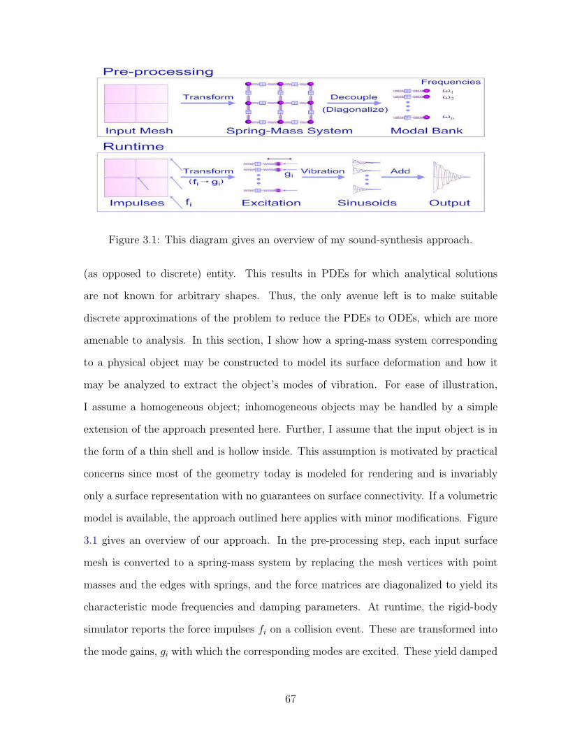
Figure 3.1: This diagram gives an overview of my sound-synthesis approach.

(as opposed to discrete) entity. This results in PDEs for which analytical solutions

are not known for arbitrary shapes. Thus, the only avenue left is to make suitable

discrete approximations of the problem to reduce the PDEs to ODEs, which are more

amenable to analysis. In this section, I show how a spring-mass system corresponding

to a physical object may be constructed to model its surface deformation and how it

may be analyzed to extract the object’s modes of vibration. For ease of illustration,

I assume a homogeneous object; inhomogeneous objects may be handled by a simple

extension of the approach presented here. Further, I assume that the input object is in

the form of a thin shell and is hollow inside. This assumption is motivated by practical

concerns since most of the geometry today is modeled for rendering and is invariably

only a surface representation with no guarantees on surface connectivity. If a volumetric

model is available, the approach outlined here applies with minor modifications. Figure

3.1 gives an overview of our approach. In the pre-processing step, each input surface

mesh is converted to a spring-mass system by replacing the mesh vertices with point

masses and the edges with springs, and the force matrices are diagonalized to yield its

characteristic mode frequencies and damping parameters. At runtime, the rigid-body

simulator reports the force impulses fi on a collision event. These are transformed into

the mode gains, gi with which the corresponding modes are excited. These yield damped

67

sinusoids which are suitably combined to yield the output sound signal.

3.1.1 Input Processing

Given an input mesh consisting of vertices and edges, an equivalent spring-mass system

is constructed by replacing the mesh vertices with point masses and the edges with

damped springs. I now discuss how to assign the spring constants and masses based on

the material properties of the object so that the discrete system closely approximates

the physical object. The spring constant, k and the particle masses, mi are given by:

k = Y t

mi = ρtai (3.1)

where Y is the Young’s Modulus of elasticity for the material, t is the thickness of the

object surface, ρ is the material density and ai is the area “covered” by a particle, which

is calculated by dividing the area of each mesh face equally amongst all its constituent

vertices and summing all the face contributions for the vertex corresponding to the

mass in consideration. Note that I did not discuss fixing the spring damping parameters

above, which I will return to shortly.

3.1.2 Deformation Modeling

Once the particle system has been constructed as above, we need to solve its equation

of motion in order to generate the corresponding sound. Unfortunately, the resulting

system of equations is still mathematically complex because the interaction forces be-

tween the masses are non-linear in their positions. However, by making the reasonable

assumption that the deformation is small and linearizing about the rest positions, this

68

problem can be cast in the form of a coupled linear system of ODEs:

Md2r

dt2+ (γM + ηK)

dr

dt+Kr = f (3.2)

where M is the mass matrix, K is the elastic force matrix, γ and η are the fluid and

viscoelastic damping constants for the material respectively. The matrix M is diagonal

with entries on the diagonal corresponding to the particle masses, mi. The elastic force

matrix K is real symmetric, with entries relating two particles if and only if they are

connected by a spring. The variable r is the displacement vector of the particles with

respect to their rest position and f is the force vector. Intuitively, the terms in the above

equation correspond to inertia, damping, elasticity and external force respectively. The

specific form of damping used above, which expresses the overall damping matrix as

a linear combination of K and M is known as Raleigh damping and works well in

practice. For a system with N particles in three dimensional space, the dimensions of

all the matrices above is 3N×3N .

This formulation of the problem is well known and is similar to the one presented

in [64]. The main difference in our approach is that the force and inertia matrices are

assembled from a spring-mass system which makes the formulation much simpler. The

solution to Equation (3.2) can be obtained by diagonalizing K so that:

K = GDG−1 (3.3)

where G is a real matrix consisting of the eigenvectors of K and D is a diagonal matrix

containing the eigenvalues. For reasons I will explain later, I will henceforth call G the

“gain matrix”. Plugging the above expression for K into Equation (3.2) and multiplying

by G−1 throughout, we obtain:

G−1Md2r

dt2+

(γG−1M + ηDG−1

) drdt

+DG−1r = f (3.4)

69

Observing that since M is diagonal, G−1M = MG−1 and defining z = G−1r equa-

tion(3.4) may be expressed as:

Md2z

dt2+ (γM + ηD)

dz

dt+Dz = G−1f (3.5)

Since both M and D in the above equation are diagonal, Equation (3.2) has been decou-

pled into a set of unrelated differential equations in the variables zi, which correspond to

individual modes of vibration of the object. The equation for each mode is the standard

equation of a damped oscillator and has the following solution for the i’th mode:

zi(t) = cieω+i t + cie

ω−i t

ω±i =

− (γλi + η)±√(γλi + η)2 − 4λi

2(3.6)

where the constant ci, called the gain for the mode, is found by considering the impulses

applied as I will discuss shortly. I use ci to denote the complex conjugate of ci. The

constant λi is the i’th eigenvalue in the diagonal matrix, D. The real part of ω±i gives

the damping coefficient for the mode, while the imaginary part, if any, gives the angular

frequency of the mode.

3.1.3 Handling Impulsive Forces

Once an input mesh has been processed as above and the corresponding modes extracted

as outlined in Equations (3.2)-(3.6), we have all the information needed regarding the

aural properties of the object. The sound produced by an object is governed by the

magnitude and location of impulsive force on its surface. Short-duration impulsive

contacts are modeled by dirac-delta functions. Given an impulse vector f containing

the impulses applied to each vertex of an object, we compute the transformed impulse,

g = G−1f in order to evaluate the right-hand side of Equation (3.5). Once this is done,

70

the equation for the i’th mode is given by:

mid2zidt2

+ (γmi + ηλi)dzidt

+ λizi = giδ(t− t0) (3.7)

where t0 is the time of collision and δ() is the dirac delta function. Integrating the above

equation from a time just before t0 to a time just after t0 and noting that∫ t+0t−0δ(t−t0)dt =

1, we obtain:

miΔ

(dzidt

)+ (γmi + ηλi)Δzi + ziΔt = gi (3.8)

Assuming that Δt is very small, and using the fact that the deformation is small com-

pared to the change in velocities, one can neglect the last two terms on the left-hand

side to obtain:

Δ

(dzidt

)=

gimi

(3.9)

The above gives a very simple rule which relates the change in the time derivative of

the mode to the transformed impulse. Referring to Equation (3.6) and requiring that zi

should stay the same just before and after the collision while dzidt

should increase as in

Equation (3.9), the update rule for the mode gain ci can be shown to be:

ci ← ci +gi

mi

(ω+i − ω−

i

)eω

+i t0

. (3.10)

Initially, ci is set to 0 for all modes.

3.2 Real-time Sound Synthesis

In this section, I describe how the mathematical formulation presented in the previous

section is utilized to efficiently generate sound in real time. First, I describe a naive

implementation and then discuss techniques to increase its efficiency.

Assume that there exists a rigid-body simulator which can handle all the dynamics.

During a collision event, the sound system is informed of the object that undergoes

71

the impact and the magnitude and location of impact. This impact is processed as

described in Section 3.1.3 to result in the gains for the different modes of vibration of

the object, where the gain for the i’th mode being ci. The equation for a mode from

the time of collision onwards is given by (3.6). The amplitude contribution of a mode

at any moment is proportional1 to its velocity (and not position). This is because the

pressure contribution of a particle is determined by its velocity and the mode velocities

are linearly related to the physical velocities of the particles. The mode velocity is found

by taking a differential of Equation (3.6) with respect to time:

vi =dzidt

= ciω+i e

ω+i t + ciω

−i e

ω−i t (3.11)

For generating each audio sample, we need to evaluate the above equation for all

vibration modes of the object, which is quite inefficient. As mentioned in [64], the simple

observation that eiω(t+Δt) = eiωteiωΔt offers some gain in performance since generating

a new audio sample just requires a single complex multiply with the previous value.

However, the efficiency is still not sufficient to handle a large number of objects in real

time. We may estimate the running time of the system as follows: A simple spring-mass

system with N particles has 3N modes, and the above operation needs to be repeated

for each mode for each audio sample. Assuming a sampling rate of 44100 Hz, the number

of floating-point operations (FLOPS) needed for this calculation for generating audio

samples worth t seconds is:

T = 3N × 4× 44100t FLOPS . (3.12)

Considering that the typical value of N is about 5000 or higher, producing sound worth

1The constant of proportionality is determined based on the geometry of the object and takes thefact into account that vibrations in the direction of the surface normal contribute more to the resultingpressure wave than vibrations perpendicular to the normal. I do not describe it in detail here as it isnot critical to the approach being presented.

72

1 second would take 2646 MFLOPS. Since today’s fastest desktop processors operate

at a few thousand MFLOPS [25], the above processing would take about a second.

Given that this estimated amount of time is for just one object and a typical scene may

contain many such objects, such an approach is clearly not fast enough for interactive

applications. Furthermore, for many real-time environments such as games and virtual

environments, only a very small fraction of the actual time can be allocated for sound

production. Thus, in the rest of this section, I will discuss techniques to increase the

efficiency of the proposed base system to enhance its capability in handling scenarios

with a large number of sounding objects at interactive rates.

From Equation (3.12), it is clear that the running time is proportional to the number

of modes being mixed and the number of objects. Next, I present acceleration techniques

for sound simulation by reducing the number of modes per object: “Mode Compression”

and “Mode Truncation”, and by scaling the audio quality of different objects dynamically

with little degradation in perceived sound quality.

3.2.1 Mode Compression

Humans have a limited range of frequency perception, ranging from 20 to 22000 Hz.

It immediately follows that modes with frequencies lying outside this range can be

clipped out and need not be mixed. However, there is another important fact which

can lead to large reductions in the number of modes to be mixed. A perceptual study

described in [92] shows that humans have a limited capacity to discriminate between

nearby frequencies. Note that this is different from frequency masking [119] in which

one of two simultaneously played frequencies masks out the other. Rather, this result

reports that even if two “close enough” frequencies are played in succession, the listener

is unable to tell whether they were two different frequencies or the same frequency

played out twice. The authors call the length of the interval of frequencies around a

center frequency which sound the same, the “Difference Limens to Change” (DLC).

73

Figure 3.2: This plot shows frequency discrimination in humans as a function of thecenter frequency. Note that the human capacity to discriminate between frequenciesdegrades considerably for frequencies in the range 2-22 KHz, which forms a bulk of thehuman audible range. I use this fact to guarantee that no more than 1000 modes needto be mixed for any object in the worst case, irrespective of its geometric complexity. Inmost cases the actual number is much smaller, in the range of a few hundreds. The redcurve shows the piecewise linear approximation of this curve that my technique uses.

Figure 3.2 shows a plot of the DLC against center frequencies ranging from .25 to 8

KHz. Interestingly, the DLC shows a large variation over the audible frequency range,

getting very large as the center frequency goes beyond 2 KHz. Even at 2 KHz, the DLC

is more than 1 Hz. That is, a human subject cannot tell apart 1999 Hz from 2000 Hz.

I exploit the above fact to drastically reduce the number of modes that are mixed

for an object. The DLC curve is approximated with a piecewise linear curve shown as

the red line in Figure 3.2. The approximation has two segments: one from 20 Hz to 2

KHz and another from 2 KHz to 22 KHz. As I show in the figure, the DLC is slightly

overestimated. This increases the performance further and I have observed minimal loss

in quality in all the cases I have tested. The main idea behind our compression scheme

is to group together all the modes with perceptually indistinguishable frequencies. It

can be easily shown that if the above mentioned linear approximation to the DLC curve

is used and indistinguishable modes clustered at the corresponding frequency centers,

74

the maximum number of modes that need to be mixed is less than 1000. It is important

to note that this is just the worst case scenario and it happens only when the frequency

spectrum of the object consists of all frequencies from 20 to 22,000 Hz, which is very

rare. For most objects, the frequency spectrum is discrete and consequently, the number

of modes after mode compression is much smaller than 1000, typically in the range of a

few hundreds.

I now describe the details of my technique. Recall the gain matrix from Equa-

tion (3.3), G. The gain matrix has a very simple physical interpretation: Rows of the

matrix correspond to vertices of the object and columns correspond to the different

modes of vibration (with their corresponding frequencies). Each row of G lists the gains

for the various modes of vibration of the object, when a unit impulse is applied on

the corresponding vertex. It is clear from the above discussion that all the mode gains

within a row of G which correspond to modes with close frequencies need to be clustered

together. This is achieved by replacing the gain entries for all such modes by a single

entry with gain equal to the sum of the constituent gains. Since a mode corresponds to

a whole column, this reduces to summing together columns element-wise based on their

frequencies. The complete procedure is as follows:

• Sort the columns of G with the corresponding mode frequencies as the key. 2

• Traverse the modes in increasing order of frequency. Estimate the DLC, Δ at

the current frequency using the piecewise linear curve shown in Figure 3.2. If the

current frequency and next frequency are within Δ of each other the two mode

frequencies are indistinguishable, replace the two columns by their element-wise

sum.

Below, I enumerate the main advantages of this scheme:

2This step is usually not needed as most linear algebra packages output the eigenvector matrix sortedon the eigenvalues

75

1. The running time is constant instead of linear in the number of vertices in the

object. For example, if the input mesh is complex with 5,000 vertices, the number

of modes mixed is bounded by 1000 instead of the earlier 3N = 15, 000 which is a

substantial performance gain.

2. Since this scheme requires just the frequencies of the different modes, the whole

processing can be done as a pre-process without requiring any extra runtime CPU

cycles.

3. From the above mentioned procedure, it is clear that the number of columns in

the matrix G, which is the same as the number of modes, is now bounded by 1000

instead of the earlier value of 3N . Since this matrix needs to be present in memory

at runtime for transforming impulses to mode gains, its memory consumption is

an important issue. Using this technique, for an object with 5000 vertices, the

memory requirement has been reduced from 225 MB to less than 15 MB, by more

than a factor of 15.

4. Most objects have a discrete frequency spectrum with possibly many degenerate

frequencies. Due to numerical inaccuracies while diagonalizing the elastic force

matrix and the approximations introduced by the spring-mass discretization, these

degenerate frequencies may appear as spurious distinct modes with near-equal

frequencies. Obviously, it is wasteful to treat these as distinct modes. It is our

observation that most of the times these modes’ frequencies are close enough so

that they are naturally summed together in this scheme.

3.2.2 Mode Truncation

The sound of a typical object on being struck consists of a transient response composed

of a blend of high frequencies, followed by a set of lower frequencies with low amplitude.

76

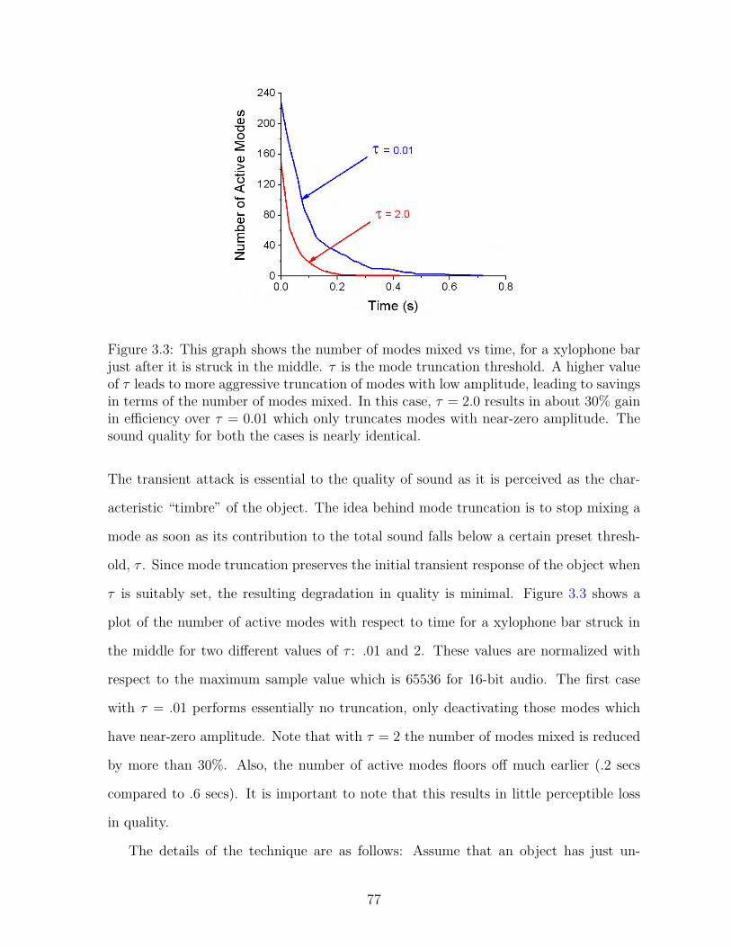
Figure 3.3: This graph shows the number of modes mixed vs time, for a xylophone barjust after it is struck in the middle. τ is the mode truncation threshold. A higher valueof τ leads to more aggressive truncation of modes with low amplitude, leading to savingsin terms of the number of modes mixed. In this case, τ = 2.0 results in about 30% gainin efficiency over τ = 0.01 which only truncates modes with near-zero amplitude. Thesound quality for both the cases is nearly identical.

The transient attack is essential to the quality of sound as it is perceived as the char-

acteristic “timbre” of the object. The idea behind mode truncation is to stop mixing a

mode as soon as its contribution to the total sound falls below a certain preset thresh-

old, τ . Since mode truncation preserves the initial transient response of the object when

τ is suitably set, the resulting degradation in quality is minimal. Figure 3.3 shows a

plot of the number of active modes with respect to time for a xylophone bar struck in

the middle for two different values of τ : .01 and 2. These values are normalized with

respect to the maximum sample value which is 65536 for 16-bit audio. The first case

with τ = .01 performs essentially no truncation, only deactivating those modes which

have near-zero amplitude. Note that with τ = 2 the number of modes mixed is reduced

by more than 30%. Also, the number of active modes floors off much earlier (.2 secs

compared to .6 secs). It is important to note that this results in little perceptible loss

in quality.

The details of the technique are as follows: Assume that an object has just un-

77

dergone a collision and the resulting mode gains ci have been calculated as given by

Equation (3.10). From this time onwards until the object undergoes another collision,

Equation (3.11) gives a closed-form expression for the mode’s contribution to the sound

of the object. This can be used to predict exactly when the mode’s contribution drops

below the threshold τ . The required “cutoff time”, tci is such that for all times t > tci :

ciω+i e

ω+i t + ciω

−i e

ω−i t < τ (3.13)

Using the fact that for any two complex numbers x and y, |x+ y| ≤ |x| + |y| it can be

shown that,

tci ≤1

−Re(ω+i )

ln

(2 |ci|

∣∣ω+i

∣∣τ

)(3.14)

Using the above inequality, the cutoff times are calculated for all the modes just after a

collision happens. While generating the sound samples from a mode, only one floating

point comparison is needed to test if the current time exceeds the cutoff time for the

mode. In case it does, the mode’s contribution lies below τ and consequently, it is not

evaluated.

3.2.3 Quality Scaling

The two techniques discussed above are aimed at increasing the efficiency of sound

synthesis for a single object. However, when the number of sounding objects in a scene

grows beyond a few tens, this approach is not efficient enough to work in real time and

it is not possible to output the sound for all the objects at the highest quality. It is

critical in most interactive applications that the sound system have a graceful way of

varying quality in response to variable time constraints. My technique achieves this

flexibility by scaling the sound quality for the objects. The sound quality of an object is

changed by controlling the number of modes being mixed for synthesizing its sound. In

most cases of scenes with many sounding objects, the user’s attention is on the objects

78

in the “foreground”, that is, the objects which contribute the most to the total sound

in terms of amplitude. Therefore, if it is ensured that the foreground sounds are mixed

at high quality while the background sounds are mixed at a relatively lower quality, the

resulting degradation in perceived aural quality should be reduced.

I use a simple scheme to ensure higher quality for the foreground sounds. At the end

of each video frame, the sum of the vibrational amplitudes of all modes for each object

are stored, which serve to determine the object’s priority. At the next video frame, all

objects are sorted in decreasing order based on their priority and the total time-quota

for sound-generation divided among the objects as a linearly decreasing ramp with a

preset slope, S. After this, all objects are processed in their priority order. For each

object, its quality is first scaled so that it can finish within its assigned time-quota and

then the required modes are mixed for the given time period. If an object finishes before

its time-quota has expired, the surplus is consumed greedily by the next higher priority

object. The slope, S of the ramp decides the degree to which the foreground sound

quality is favored over a degradation in background sound quality. The case with S = 0

corresponds to no priority scheduling at all, with the time-quota being divided equally

among all objects. The converse case with S = ∞ corresponds to greedy consumption

of the time-quota. That is, the whole time-quota is assigned to the highest priority

object. After the object is done, the remaining time, if any, is assigned to the next

highest priority object and so on.

3.2.4 Putting Everything Together

To illustrate how all the techniques described above are integrated, I present a summary

of my approach.

Pre-processing

• Construct a spring-mass system corresponding to the input mesh. (Section 3.1.1)

79

• Process the spring-mass system to extract the gain matrix, G and the (complex)

angular frequencies of the object’s modes of vibration: ω+i and ω−

i . (Section 3.1.2,

Eqns. (3.3) and (3.6))

• Mode Compression:

Aggregate columns of G based on frequencies of the corresponding modes, as

described in Section 3.2.1.

• Store the resulting gain matrix along with the (complex) constants ω+i and ω−

i for

modes correspond to the columns of G after compression. Note that ω−i need not

be stored in case ω+i has a non-zero imaginary part since in that case ω−

i = ω+i .

Runtime Processing

• Load the gain matrix and mode data for each object.

• Begin simulation loop:

1. Run rigid-body simulation

2. For each object, O:

– Collision Handling:

If the rigid-body simulator reports that O undergoes a collision event,

update its gain coefficients as per Equation (3.10) using the collision

impulse and its location. (Section 3.1.3)

– Mode Truncation:

Compute cutoff times tcj for each mode based on the mode truncation

threshold, τ . (Section 3.2.2, Equation (3.14))

3. Quality Scaling:

Sort objects based on amplitude contribution, assign time-quotas and com-

pute the number of modes to be mixed for each object. (Section 3.2.3)

80

4. Sound Synthesis:

For each timestep at time t and for each object, O:

– Consider all modes permitted by the current quality setting which sat-

isfy tcj > t. Sample and summate all these modes as described at the

beginning of this section. This is O’s contribution to the sound.

– Output the sum of all objects’ sample contribution as the sound sample

for time t.

End simulation loop

3.3 Implementation and Results

In this section I present results to demonstrate the efficiency and realism achievable with

our approach.

3.3.1 Rigid Body Simulation

I have implemented the algorithm and acceleration techniques presented in this chapter

using C++ and OpenGL. The rigid-body simulator extends the technique presented by

Guendelman et al. [37] to incorporate DEEP [46] for fast and more accurate penetration

depth estimation, instead of sample-based estimation using distance fields. It also uses

a more complex friction model presented by Mirtich and Canny [59], which results in

more robust contact resolution. More recently, I have also integrated this system with

the Open Dynamics Engine (ODE), as well as the NVIDIA PhysX engine, showing that

the sound system doesn’t put any special requirements on the physics engine and works

with present-day game technology.

A video containing synthesized sounds for all the tests described below can be found

at the website: http://gamma.cs.unc.edu/symphony.

81

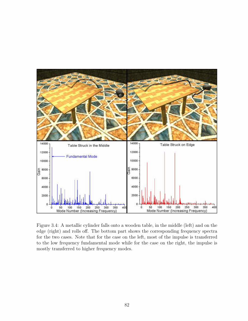
Figure 3.4: A metallic cylinder falls onto a wooden table, in the middle (left) and on theedge (right) and rolls off. The bottom part shows the corresponding frequency spectrafor the two cases. Note that for the case on the left, most of the impulse is transferredto the low frequency fundamental mode while for the case on the right, the impulse ismostly transferred to higher frequency modes.

82

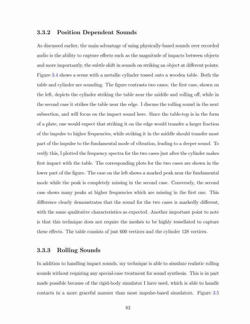
3.3.2 Position Dependent Sounds

As discussed earlier, the main advantage of using physically-based sounds over recorded

audio is the ability to capture effects such as the magnitude of impacts between objects

and more importantly, the subtle shift in sounds on striking an object at different points.

Figure 3.4 shows a scene with a metallic cylinder tossed onto a wooden table. Both the

table and cylinder are sounding. The figure contrasts two cases: the first case, shown on

the left, depicts the cylinder striking the table near the middle and rolling off, while in

the second case it strikes the table near the edge. I discuss the rolling sound in the next

subsection, and will focus on the impact sound here. Since the table-top is in the form

of a plate, one would expect that striking it on the edge would transfer a larger fraction

of the impulse to higher frequencies, while striking it in the middle should transfer most

part of the impulse to the fundamental mode of vibration, leading to a deeper sound. To

verify this, I plotted the frequency spectra for the two cases just after the cylinder makes

first impact with the table. The corresponding plots for the two cases are shown in the

lower part of the figure. The case on the left shows a marked peak near the fundamental

mode while the peak is completely missing in the second case. Conversely, the second

case shows many peaks at higher frequencies which are missing in the first one. This

difference clearly demonstrates that the sound for the two cases is markedly different,

with the same qualitative characteristics as expected. Another important point to note

is that this technique does not require the meshes to be highly tessellated to capture

these effects. The table consists of just 600 vertices and the cylinder 128 vertices.

3.3.3 Rolling Sounds

In addition to handling impact sounds, my technique is able to simulate realistic rolling

sounds without requiring any special-case treatment for sound synthesis. This is in part

made possible because of the rigid-body simulator I have used, which is able to handle

contacts in a more graceful manner than most impulse-based simulators. Figure 3.5

83

Figure 3.5: A plot of the impulses on a cylinder versus time for the scene shown onthe right in Figure 3.4 and the corresponding audio samples. The peaks correspond toimpacts while the numerous low-amplitude impulses correspond to rolling forces.

shows the impulses on the cylinder and the corresponding audio for the case shown in

the right side of Figure 3.4. The cylinder rolls on the table after impact, falls to the

ground and rolls on the floor for sometime. The initial rolling sound, when the cylinder is

on the table, has a much richer quality. The sound of the table as the cylinder rolls over

it conveys a sense of the cylinder’s heaviness, which is only partly conveyed by the sound

of the impact. The cylinder, although uniformly tessellated, is very coarse, with only

32 circumferential subdivisions. Figure 3.5 shows the impulses applied on the cylinder

against time. The peaks correspond to impacts: when the cylinder falls on the table,

and when it falls to the ground from the table. Note that the audio waveform shows

the corresponding peaks correctly. The period of time stretching from 6 to 8 seconds

consists of the cylinder rolling on the floor and is characterized by many closely-spaced

small-magnitude impulses on the cylinder as it strikes the floor again and again due

to its tessellation. To test how important the periodicity of these impulses was for the

realism of rolling sounds, the mean and standard deviation of the interval between these

impulses were computed from the data presented in Figure 3.5. The mean time between

84

the impulses was 17 ms with a standard deviation of 10 ms. The fact that the standard

deviation is more than 50% of the mean demonstrates that the impulses show very little

periodicity. This seems to suggest that the periodicity of collisions is not critical for the

perceived realism of rolling sounds.

3.3.4 Efficiency

My technique is able to perform sound synthesis for complex scenes in real time. Figure

3.6 shows a scene with 100 metallic rings falling simultaneously onto a wooden table

and undergoing elastic collision. All the rings and the table are sounding. Each ring

is treated as a separate object with separate aural properties. The rings consist of 200

vertices each. Figure 3.7 shows the audio FPS3 for this simulation against time for the

one second interval during which almost all the collisions take place. The application

frame rate is 100 FPS. Note that this is not the raw data but a moving average so that

the short-range fluctuations are absorbed. The plot on the bottom is the base timing

without using any of the acceleration techniques described in Section 4. The audio in

this case is very choppy since the audio generation is not able to keep up with the speed

of rendering and rigid-body simulation. With mode truncation and mode compression,

the performance shows significant improvement. However, after initially starting at

about 200 FPS, the frame rate drops in the latter part where the maximum number of

collisions happen. With quality scaling in addition to mode compression and truncation

(shown by the top-most curve), the frame rate exhibits no such drop, continuing to be

around 200 FPS. This is because quality scaling gives priority to sound generation for

those rings which just underwent collision, while lowering the quality for other rings

which may have collided earlier and are contributing less to the overall sound. This

illustrates the importance of quality scaling for scenarios with multiple collisions. It is

3An audio frame is defined as the amount of sound data sufficient to play for a duration equal tothe duration of one video frame.

85

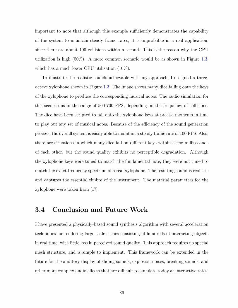
important to note that although this example sufficiently demonstrates the capability

of the system to maintain steady frame rates, it is improbable in a real application,

since there are about 100 collisions within a second. This is the reason why the CPU

utilization is high (50%). A more common scenario would be as shown in Figure 1.3,

which has a much lower CPU utilization (10%).

To illustrate the realistic sounds achievable with my approach, I designed a three-

octave xylophone shown in Figure 1.3. The image shows many dice falling onto the keys

of the xylophone to produce the corresponding musical notes. The audio simulation for

this scene runs in the range of 500-700 FPS, depending on the frequency of collisions.

The dice have been scripted to fall onto the xylophone keys at precise moments in time

to play out any set of musical notes. Because of the efficiency of the sound generation

process, the overall system is easily able to maintain a steady frame rate of 100 FPS. Also,

there are situations in which many dice fall on different keys within a few milliseconds

of each other, but the sound quality exhibits no perceptible degradation. Although

the xylophone keys were tuned to match the fundamental note, they were not tuned to

match the exact frequency spectrum of a real xylophone. The resulting sound is realistic

and captures the essential timbre of the instrument. The material parameters for the

xylophone were taken from [17].

3.4 Conclusion and Future Work

I have presented a physically-based sound synthesis algorithm with several acceleration

techniques for rendering large-scale scenes consisting of hundreds of interacting objects

in real time, with little loss in perceived sound quality. This approach requires no special

mesh structure, and is simple to implement. This framework can be extended in the

future for the auditory display of sliding sounds, explosion noises, breaking sounds, and

other more complex audio effects that are difficult to simulate today at interactive rates.

86

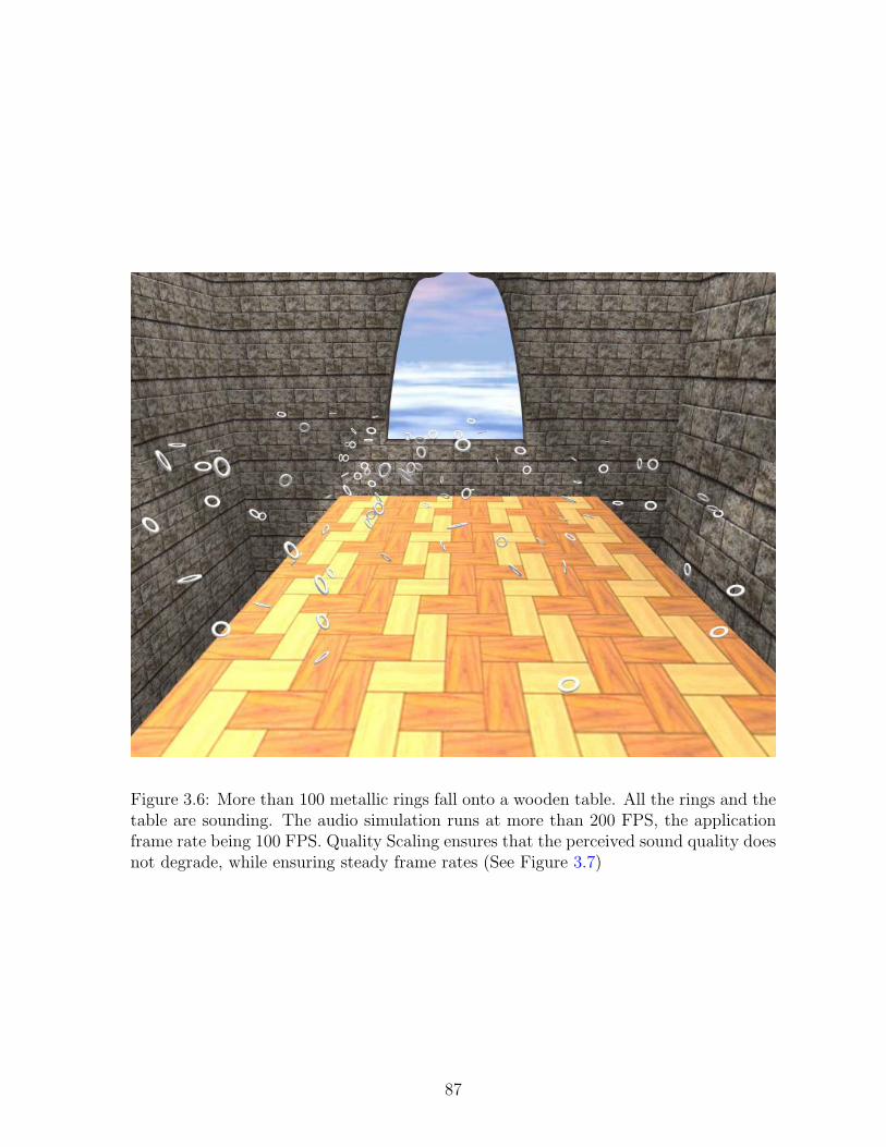
Figure 3.6: More than 100 metallic rings fall onto a wooden table. All the rings and thetable are sounding. The audio simulation runs at more than 200 FPS, the applicationframe rate being 100 FPS. Quality Scaling ensures that the perceived sound quality doesnot degrade, while ensuring steady frame rates (See Figure 3.7)

87

Figure 3.7: This graph shows the audio simulation FPS for the scene shown in Figure 3.6from time 1s to 2s, during which almost all the collisions take place. The bottom-mostplot shows the FPS for an implementation using none of the acceleration techniques.The top-most curve shows the FPS with mode compression, mode truncation and qualityscaling. Note how the FPS stays near 200 even when the other two curves dip due tonumerous collisions during 1.5-2.0s.

88

Chapter 4

Efficient Numerical Acoustics

In this chapter, I discuss my work on performing efficient numerical acoustics simulation

on large scenes. I begin with a discussion of the mathematical background and describe

in some detail, a high-accuracy finite-difference scheme, FDTD (Finite Difference Time

Domain). In the next section, I describe my adaptive rectangular decomposition (ARD)

approach. Following this, I describe the results obtained with my technique, as well as

a discussion of the errors and performance. Finally, I conclude with a summary of my

work and a discussion of possible future work in this area.

4.1 Mathematical Background

In this section, I discuss the FDTD method. I do this for two reasons: Firstly, this is

the simulator I use as a reference to compare against and its details serve to illustrate

the underlying mathematical framework used throughout this chapter. Secondly, this

discussion illustrates numerical dispersion errors in FDTD and motivates our technique

which uses the analytical solution to the Wave Equation on rectangular domains to

remove numerical dispersion errors.

4.1.1 Basic Formulation

The input to an acoustics simulator is a scene in 3D, along with the boundary conditions

and the locations of the sound sources and listener. The propagation of sound in a

domain is governed by the Acoustic Wave Equation,

∂2p

∂t2− c2∇2p = F (x, t) , (4.1)

This equation captures the complete wave nature of sound, which is treated as a time-

varying pressure field p (x, t) in space. The speed of sound is c = 340ms−1 and F (x, t)

is the forcing term corresponding to sound sources present in the scene. The operator

∇2 = ∂2

∂x2 +∂2

∂y2+ ∂2

∂z2is the Laplacian in 3D. The Wave Equation succinctly explains wave

phenomena such as interference and diffraction that are observed in reality. I briefly

mention a few physical quantities and their relations, which will be used throughout

the chapter. For a wave traveling in free space, the frequency, ν and wavelength, λ

are related by c = νλ. It is also common to use the angular counterparts of these

quantities: angular frequency, ω = 2πν and wavenumber, k = 2πλ. Because frequency

and wavenumber are directly proportional to each other, I will be using the two terms

interchangeably throughout the chapter.

In the next sub-section, I briefly discuss the Finite Difference Time Domain (FDTD)

method for numerically solving the Wave Equation. To avoid confusion, I note here that

while the term FDTD is sometimes used to specifically refer to the original algorithm

proposed by Yee [116] for Electromagnetic simulation, it is common to refer to any Finite

Difference-based approach which computes the complete sound field in time domain as

an FDTD method. In this chapter, I use the latter definition.

90

4.1.2 A (2,6) FDTD Scheme

FDTD works on a uniform grid with spacing h. To capture the propagation of a pre-

scribed maximum frequency νmax, the Nyquist theorem requires that h ≤ λmax

2= c

2νmax.

Once the spatial discretization is performed, the continuum Laplacian operator is re-

placed with a discrete approximation of desired order of accuracy. Throughout this

chapter, I consider the sixth order accurate approximation to the Laplacian, which ap-

proximates the second order differential in each dimension with the following stencil:

d2pidx2

≈ 1

180h2(2pi−3 − 27pi−2 + 270pi−1 − 490pi

+270pi+1 − 27pi+2 + 2pi+3) +O(h6), (4.2)

where pi is the ith grid cell in the corresponding dimension. Thus, the Laplacian operator

at each cell can be represented as a Discrete Laplacian Matrix, K and equation (4.1)

becomes,

∂2P

∂t2− c2

h2KP = F (t) , (4.3)

where P is a long vector listing the pressure values at all the grid cells and F is the

forcing term at each cell. Hard-walls may be modeled with the Neumann Boundary

Condition – ∂p∂n

= 0, where n is the normal to the boundary.

The next step is to discretize equation (4.3) in time at some time-step Δt, which is

restricted by the CFL condition Δt < hc√3. Using the Leapfrog integrator in time, the

complete update rule is as follows.

P n+1 = 2P n − P n−1 +

(cΔt

h

)2

KP n +O(Δt2

)+O

(h6

).

Since the temporal and spatial errors are second and sixth order respectively, this is

a (2,6) FDTD scheme. In the next sub-section, I discuss the nature of the numerical

errors in FDTD schemes and the resulting performance issues.

91

4.1.3 Numerical Dispersion in FDTD and Efficiency Consider-

ations

As was previously discussed, the spatial cell size, h for FDTD is chosen depending on

the maximum simulated frequency, νmax and is limited by the Nyquist sampling theo-

rem. However, due to numerical errors arising from spatial and temporal discretization,

accurate simulation with FDTD typically requires not 2 but 8-10 samples per wave-

length [99]. These errors manifest themselves in the form of Numerical Dispersion –

Waves with different wavenumbers (or equivalently, different frequencies) do not travel

with the same speed in the simulation. This error may be quantified by finding the

wavenumber-dependent numerical speed, c′ (k), where k is the wavenumber. This speed

is then normalized by dividing with the ideal wave speed, c, yielding the dispersion co-

efficient, γ (k). Ideally, the dispersion coefficient should be as close to 1 as possible, for

all wavenumbers. Figure 4.1 shows a plot of the dispersion coefficient for FDTD against

frequency on a 3D grid and compares the error for different cell sizes. Observe that at

1000 Hz, the dispersion coefficient for FDTD is about .01c, while for FDTD running

on a 2.5× refined mesh the error is about .001c. This is because the spatial sampling

increases from 4 samples per wavelength to 10 samples per wavelength.

Consider a short-time signal containing many frequencies, for example, a spoken

consonant. Due to Numerical Dispersion, each of the frequencies in the consonant will

travel with a slightly different speed. As soon as the phase relations between different

frequencies are lost, the signal is effectively destroyed and the result is a muffled sound.

From the above values of the dispersion coefficient, it can be shown that with FDTD a

signal would have lost phase coherence after traveling just 17m, which is comparable to

the diameter of most scenes.

To increase accuracy, the mesh resolution needs to be increased, but that greatly

increases the compute and memory requirements of FDTD – Refining the mesh r times

implies an increase on memory by a factor of r3 and the total compute time for a given

92

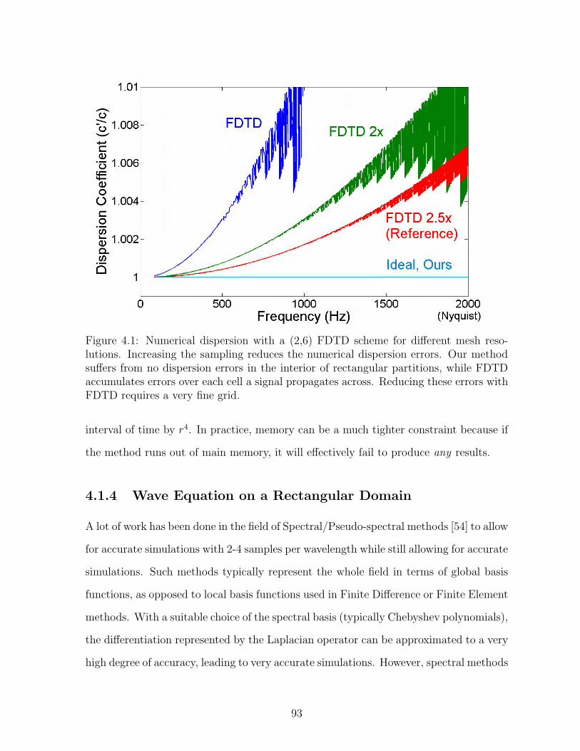
Figure 4.1: Numerical dispersion with a (2,6) FDTD scheme for different mesh reso-lutions. Increasing the sampling reduces the numerical dispersion errors. Our methodsuffers from no dispersion errors in the interior of rectangular partitions, while FDTDaccumulates errors over each cell a signal propagates across. Reducing these errors withFDTD requires a very fine grid.

interval of time by r4. In practice, memory can be a much tighter constraint because if

the method runs out of main memory, it will effectively fail to produce any results.

4.1.4 Wave Equation on a Rectangular Domain

A lot of work has been done in the field of Spectral/Pseudo-spectral methods [54] to allow

for accurate simulations with 2-4 samples per wavelength while still allowing for accurate

simulations. Such methods typically represent the whole field in terms of global basis

functions, as opposed to local basis functions used in Finite Difference or Finite Element

methods. With a suitable choice of the spectral basis (typically Chebyshev polynomials),

the differentiation represented by the Laplacian operator can be approximated to a very

high degree of accuracy, leading to very accurate simulations. However, spectral methods

93

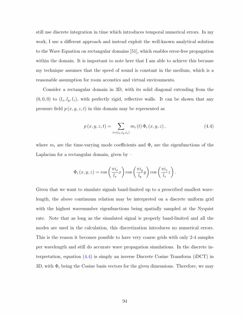
still use discrete integration in time which introduces temporal numerical errors. In my

work, I use a different approach and instead exploit the well-known analytical solution

to the Wave Equation on rectangular domains [51], which enables error-free propagation

within the domain. It is important to note here that I am able to achieve this because

my technique assumes that the speed of sound is constant in the medium, which is a

reasonable assumption for room acoustics and virtual environments.

Consider a rectangular domain in 3D, with its solid diagonal extending from the

(0, 0, 0) to (lx, ly, lz), with perfectly rigid, reflective walls. It can be shown that any

pressure field p (x, y, z, t) in this domain may be represented as

p (x, y, z, t) =∑

i=(ix,iy ,iz)

mi (t) Φi (x, y, z) , (4.4)

where mi are the time-varying mode coefficients and Φi are the eigenfunctions of the

Laplacian for a rectangular domain, given by –

Φi (x, y, z) = cos

(πixlx

x

)cos

(πiyly

y

)cos

(πizlz

z

).

Given that we want to simulate signals band-limited up to a prescribed smallest wave-

length, the above continuum relation may be interpreted on a discrete uniform grid

with the highest wavenumber eigenfunctions being spatially sampled at the Nyquist

rate. Note that as long as the simulated signal is properly band-limited and all the

modes are used in the calculation, this discretization introduces no numerical errors.

This is the reason it becomes possible to have very coarse grids with only 2-4 samples

per wavelength and still do accurate wave propagation simulations. In the discrete in-

terpretation, equation (4.4) is simply an inverse Discrete Cosine Transform (iDCT) in

3D, with Φi being the Cosine basis vectors for the given dimensions. Therefore, we may

94

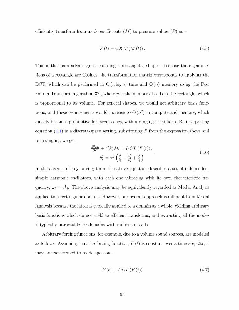
efficiently transform from mode coefficients (M) to pressure values (P ) as –

P (t) = iDCT (M (t)) . (4.5)

This is the main advantage of choosing a rectangular shape – because the eigenfunc-

tions of a rectangle are Cosines, the transformation matrix corresponds to applying the

DCT, which can be performed in Θ (n log n) time and Θ (n) memory using the Fast

Fourier Transform algorithm [32], where n is the number of cells in the rectangle, which

is proportional to its volume. For general shapes, we would get arbitrary basis func-

tions, and these requirements would increase to Θ (n2) in compute and memory, which

quickly becomes prohibitive for large scenes, with n ranging in millions. Re-interpreting

equation (4.1) in a discrete-space setting, substituting P from the expression above and

re-arranging, we get,

∂2Mi

∂t2+ c2k2

iMi = DCT (F (t)) ,

k2i = π2

(i2xl2x+

i2yl2y+ i2z

l2z

) . (4.6)

In the absence of any forcing term, the above equation describes a set of independent

simple harmonic oscillators, with each one vibrating with its own characteristic fre-

quency, ωi = cki. The above analysis may be equivalently regarded as Modal Analysis

applied to a rectangular domain. However, our overall approach is different from Modal

Analysis because the latter is typically applied to a domain as a whole, yielding arbitrary

basis functions which do not yield to efficient transforms, and extracting all the modes

is typically intractable for domains with millions of cells.

Arbitrary forcing functions, for example, due to a volume sound sources, are modeled

as follows. Assuming that the forcing function, F (t) is constant over a time-step Δt, it

may be transformed to mode-space as –

F (t) ≡ DCT (F (t)) (4.7)

95

and one may derive the following update rule –

Mn+1i = 2Mn

i cos (ωiΔt)−Mn−1i +

2F n

ω2i

(1− cos (ωiΔt)) . (4.8)

This update rule is obtained by using the closed form solution of a simple harmonic

oscillator over a time-step. Since it is a second-order equation, we need to specify one

more initial condition, which I choose to be that the function computed over the time-

step evaluates correctly to the value at the previous time-step, Mn−1. This leads to a

time-stepping scheme which has no numerical errors for propagation in the interior of

the rectangle, since we are directly using the closed-form solution for a simple harmonic

oscillator. The only error introduced is in assuming that the forcing term is constant

over a time-step. This is not a problem for input source sounds, as the time-step is

necessarily below the sampling rate of the input signal. However, the communication

of sound between two rectangular domains is ensured through forcing terms on their

interface and this approximation introduces numerical errors at the interface. I discuss

these issues in detail in the next section.

4.2 Technique

In the previous section, I discussed the errors and efficiency issues of the FDTD method

and discussed a method to carry out numerical solution of the Wave Equation accurately

and efficiently on rectangular domains. In this section, I discuss my technique which

exploits these observations to perform acoustic simulation on arbitrary domains by de-

composing them into rectangular partitions. I end with a discussion of the numerical

errors in my approach.

96

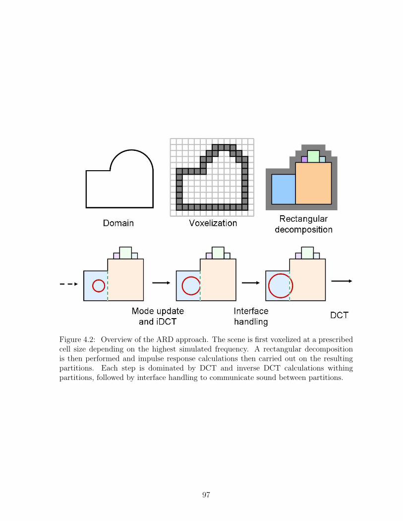
Figure 4.2: Overview of the ARD approach. The scene is first voxelized at a prescribedcell size depending on the highest simulated frequency. A rectangular decompositionis then performed and impulse response calculations then carried out on the resultingpartitions. Each step is dominated by DCT and inverse DCT calculations withingpartitions, followed by interface handling to communicate sound between partitions.

97

4.2.1 Adaptive Rectangular Decomposition

Most scenes of interest for the purpose of acoustic simulation necessarily have large

empty spaces in their interior. Consider a large scene like, for example, a 30m high

cathedral in which an impulse is triggered near the floor. With FDTD, this impulse

would travel upwards and would accumulate numerical dispersion error at each cell

it crosses. Given that the spatial step size is comparable to the wavelength of the

impulse, which is typically a few centimeters, the impulse accumulates a lot of error while

crossing hundreds to thousands of cells. In the previous section, I discussed that wave

propagation on a rectangular domain can be performed very efficiently while introducing

no numerical errors. If we fit a rectangle in the scene extending from the bottom to

the top, the impulse would have no propagation error. This is the chief motivation for

Rectangular Decomposition – Since there are large empty spaces in typical scenes, a

decomposition of the space into rectangular partitions would yield many partitions with

large volume and exact propagation could be performed in the interior of each.

The rectangular decomposition is performed by first voxelizing the scene. The cell

size is chosen based on the maximum frequency to be simulated, as discussed previously.

Next, the rectangular decomposition is performed using a greedy heuristic, which tries

to find the largest rectangle it can grow from a random seed cell until all free cells

are exhausted. I note here that the correctness of our technique does not depend on

the optimality of the rectangular decomposition. A slightly sub-optimal partitioning

with larger interface area affects the performance only slightly, as the interface area is

roughly proportional to the surface area of the domain, while the runtime performance is

dominated by the cost of DCT, which is performed on input proportional to the volume

of the domain.

98

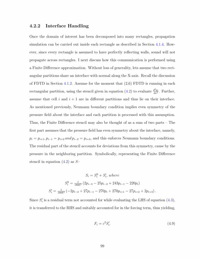
4.2.2 Interface Handling

Once the domain of interest has been decomposed into many rectangles, propagation

simulation can be carried out inside each rectangle as described in Section 4.1.4. How-

ever, since every rectangle is assumed to have perfectly reflecting walls, sound will not

propagate across rectangles. I next discuss how this communication is performed using

a Finite Difference approximation. Without loss of generality, lets assume that two rect-

angular partitions share an interface with normal along the X-axis. Recall the discussion

of FDTD in Section 4.1.2. Assume for the moment that (2,6) FDTD is running in each

rectangular partition, using the stencil given in equation (4.2) to evaluate d2pidx2 . Further,

assume that cell i and i + 1 are in different partitions and thus lie on their interface.

As mentioned previously, Neumann boundary condition implies even symmetry of the

pressure field about the interface and each partition is processed with this assumption.

Thus, the Finite Difference stencil may also be thought of as a sum of two parts – The

first part assumes that the pressure field has even symmetry about the interface, namely,

pi = pi+1, pi−1 = pi+2 and pi−2 = pi+3, and this enforces Neumann boundary conditions.

The residual part of the stencil accounts for deviations from this symmetry, cause by the

pressure in the neighboring partition. Symbolically, representing the Finite Difference

stencil in equation (4.2) as S–

Si = S0i + S ′

i, where

S0i = 1

180h2 (2pi−3 − 25pi−2 + 243pi−1 − 220pi)

S ′i =

1180h2 (−2pi−2 + 27pi−1 − 270pi + 270pi+1 − 27pi+2 + 2pi+3) .

Since S ′i is a residual term not accounted for while evaluating the LHS of equation (4.3),

it is transferred to the RHS and suitably accounted for in the forcing term, thus yielding,

Fi = c2S ′i. (4.9)

99

Similar relations for the forcing term may be derived for all cells near the partition

boundary which index cells in neighboring partitions. If I was actually using (2,6)

FDTD in each partition, this forcing term would be exact, with the same numerical

errors due to spatial and temporal approximations appearing in the interior as well

as the interface. However, because an exact solution is being used in the interior,

the interface handling described above introduces numerical errors on the interface.

I will discuss these errors in more detail shortly. I would like to note here that a

sixth-order scheme was chosen as it gives sufficiently low interface errors, while being

reasonably efficient. Lower (second/fourth) order schemes would be more efficient and

much easier to implement, but as I have experimented, they result in much higher errors,

which results in undesirable, audible high frequency noise. One may use an even higher

order scheme if more accuracy is required for a particular application, at the expense

of computation and implementaion effort. An interesting point to note at this point is

that the interface handling doesn’t need to know how the field inside each partition is

being updated. Therefore, it is easy to mix different techniques for wave propagation in

different parts of the domain, if so required.

4.2.3 Domain Decompositon Method and ARD

I now discuss my work in conext of the Domain Decomposition Method (DDM). This

serves to illuminate the choices in ARD, its novel aspects, the main source of error,

and ways to address it. Interestingly, the main motivation of the DDM when it was

conceptualized more than a century ago was very similar in spirit to my approach –

divide the domain into simpler-shaped partitions which could be analyzed more easily

[22]. However, since then, in nearly all DDM approaches for wave propagation the

principal goal has been to divide and parallelize the workload across multiple processors.

Therefore, the chief requirement in such cases is that the partitions be of near-equal size

and have minimal interface area, since such decomposition corresponds to balancing the

100

computation and minimizing the communication cost between processors.

The motivation of ARD for partitioning the domain is different – it is done to ensure

that the partitions have a particular rectangular shape even if that implies partitions

with highly varying sizes. This is because the rectangular shape yields to analytical

solution, which in turn means reduced computation without compromising numerical

accuracy for propagation within the partitions. This holds independently of any paral-

lelization considerations, which have been the main focus of prior work on wave-solvers

in high-performance computing. However, by virtue of having performed a decomposi-

tion, parallelism is still present to be exploited in ARD. I have pursued this direction to

some extent by off-loading the computed-intensive per-partition FFTs to the GPU, as

will be described later in this chapter. It is possible to parallelize my approach further

by allocating the partitions to different cores or machines, and doing interface handling

between them, and would be the way to scale ARD to very large scenes with billions of

cells, just as with other DDM approaches. I am part of current work in this direction [57]

which has already shown promising speedups of nearly ten times compared to the results

I present in this thesis. Thus, decomposing the domain into partitions and performing

interface handling between them are very well-known techniques that are applicable to

ARD, but are not the novel contribution of this work – which is the restriction of the

partition shape to rectangles and exploitation of analytical solutions.

Another interesting question is whether the existing principles of DDM can be ap-

plied directly for performing the interface handling between partitions. Most DDM

approaches have been designed for elliptic equations and require a global iterative solu-

tion where each partition is updated multiple times before reaching the final, globally-

consistent solution. The time-domain wave equation, on the other hand, is hyperbolic.

It turns out that using an explicit time-stepping scheme with the wave equation elimi-

nates the need for global iteration. Thus, in order to ensure global consistency at each

time-step with explicit wave equation solvers, including ARD, it is sufficient to apply

101

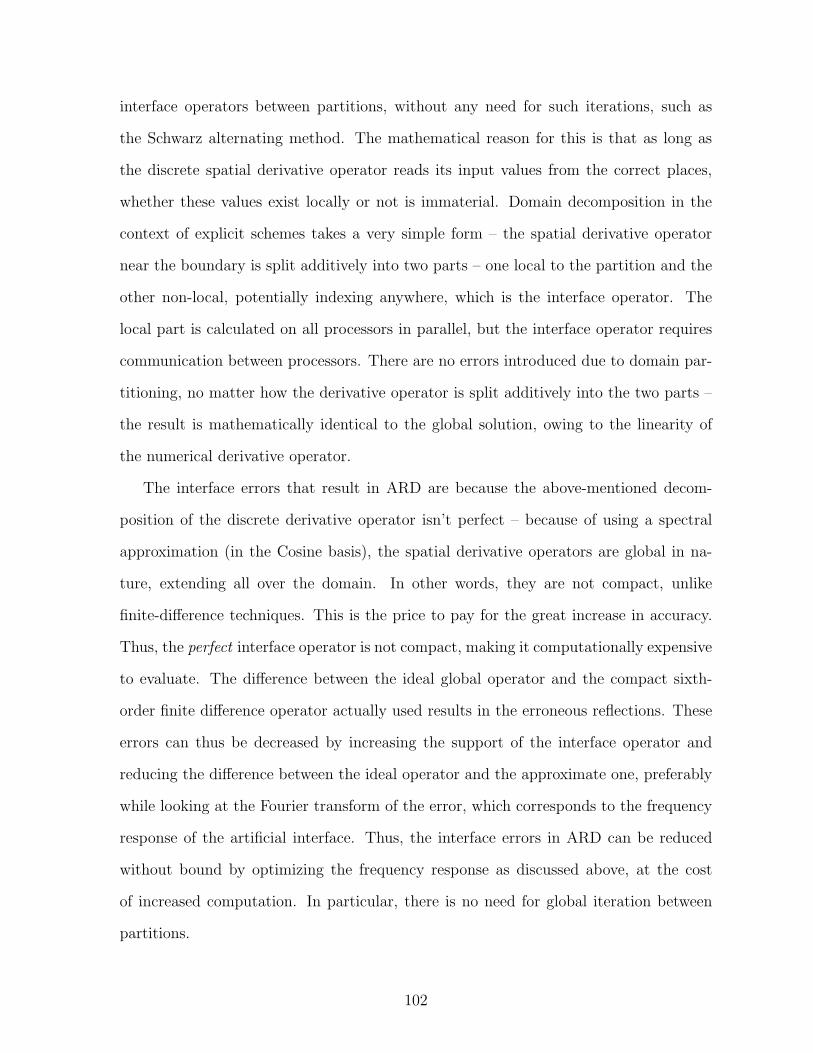
interface operators between partitions, without any need for such iterations, such as

the Schwarz alternating method. The mathematical reason for this is that as long as

the discrete spatial derivative operator reads its input values from the correct places,

whether these values exist locally or not is immaterial. Domain decomposition in the

context of explicit schemes takes a very simple form – the spatial derivative operator

near the boundary is split additively into two parts – one local to the partition and the

other non-local, potentially indexing anywhere, which is the interface operator. The

local part is calculated on all processors in parallel, but the interface operator requires

communication between processors. There are no errors introduced due to domain par-

titioning, no matter how the derivative operator is split additively into the two parts –

the result is mathematically identical to the global solution, owing to the linearity of

the numerical derivative operator.

The interface errors that result in ARD are because the above-mentioned decom-

position of the discrete derivative operator isn’t perfect – because of using a spectral

approximation (in the Cosine basis), the spatial derivative operators are global in na-

ture, extending all over the domain. In other words, they are not compact, unlike

finite-difference techniques. This is the price to pay for the great increase in accuracy.

Thus, the perfect interface operator is not compact, making it computationally expensive

to evaluate. The difference between the ideal global operator and the compact sixth-

order finite difference operator actually used results in the erroneous reflections. These

errors can thus be decreased by increasing the support of the interface operator and

reducing the difference between the ideal operator and the approximate one, preferably

while looking at the Fourier transform of the error, which corresponds to the frequency

response of the artificial interface. Thus, the interface errors in ARD can be reduced

without bound by optimizing the frequency response as discussed above, at the cost

of increased computation. In particular, there is no need for global iteration between

partitions.

102

4.2.4 Absorbing Boundary Condition

Our discussion till this point has assumed that all scene boundaries are perfectly reflect-

ing. For modeling real scenes, this is an unrealistic assumption. Moreover, since the

computation is carried out on a volumetric grid, it is necessary to truncate the domain

and model emission into free space. It is necessary to have absorbing boundaries for

this purpose. For this work, I have implemented the Perfectly Matched Layer (PML)

absorber [77], which is commonly employed in most numerical wave propagation simu-

lations due to its high absorption efficiency. PML works by applying an absorbing layer

which uses coordinate stretching to model wave propagation in an unphysical medium

with very high absorption, while ensuring that the impedance of the medium matches

that of air at the interface to avoid reflection errors. The interfacing between the PML

medium and a partition in our method is simple to implement – Since PML explic-

itly maintains a pressure field in the absorbing medium, the PML medium can also be

treated as a partition and the same technique described above can be applied for the

coupling between PML and other partitions. Variable reflectivity can be easily obtained

by multiplying the forcing term calculated for interface handling by a number between

0 and 1, 0 corresponding to full reflectivity and 1 corresponding to full absorption.

PML is very well-suited for modeling full absorption at openings in the scene, such as

doors or windows. However, because ARD employs PML for modeling partial reflections

at scene boundaries as well, it is not able to model frequency-dependent absorption. It

is entirely possible to use different boundary-handling schemes in much the same way

as it is done for FDTD. Specifically, future investigations into using techniques such as

digital impedance filters [49, 90] with ARD will allow for modeling boundary impedance

more accurately. Such integration might also offer the additional benefit of reduced

computation in boundary handling, since PML is known to be quite computationally

expensive. Therefore, I do not expect that the speedups presented in this thesis will not

be decreased by such an integration.

103

4.2.5 Putting everything together

In this subsection, I give a step-by-step description of all the steps involved in our

technique. Figure 4.2 shows a schematic diagram of the different steps in my approach,

which are as follows –

1. Pre-processing

(a) Voxelize the scene. The cell-size is fixed by the minimum simulated wave-

length and the required number of spatial samples per wavelength (typically

2-4)

(b) Perform a rectangular decomposition on the resulting voxelization, as de-

scribed in Section 4.2.1.

(c) Perform any necessary pre-computation for the DCTs to be performed at

runtime. Compute all interfaces and the partitions that share them.

2. Simulation Loop

(a) Update modes within each partition using equation (4.8)

(b) Transform all modes to pressure values by applying an iDCT as given in

equation (4.5)

(c) Compute and accumulate forcing terms for each cell. For cells on the in-

terface, use equation (4.9), and for cells with point sources, use the sample

value.

(d) Transform forcing terms back to modal space using a DCT as given in equa-

tion (4.7).

4.2.6 Numerical Errors

Numerical errors in our method are introduced mainly through two sources – boundary

approximation and interface errors. Since I employ a rectangular decomposition to

104

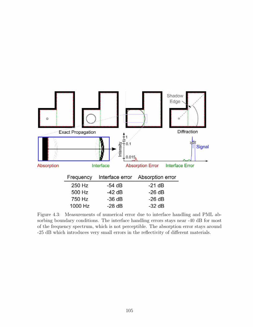
Figure 4.3: Measurements of numerical error due to interface handling and PML ab-sorbing boundary conditions. The interface handling errors stays near -40 dB for mostof the frequency spectrum, which is not perceptible. The absorption error stays around-25 dB which introduces very small errors in the reflectivity of different materials.

105

approximate the simulation domain, there are stair-casing errors near the boundary

(see Figure 4.6). These stair-casing errors are identical to those in FDTD because my

technique does a rectangular decomposition of a uniform Cartesian grid – there is no

additional geometry-approximation error due to using rectangular partitions. In most

room acoustic software, it is common practice to approximate the geometry to varying

degrees [94]. The reason for doing this is that we are not as sensitive to acoustic detail

as much as we are to visual detail. Geometric features comparable or smaller than

the wavelength of sound ( 34 cm at 1kHz) lead to very small variations in the overall

acoustics of the scene due to the presence of diffraction. In contrast, in light simulation,

all geometric details are visible because of the ultra-small wavelength of light and thus

stair-casing is a much more important problem.

The net effect of stair-casing error for numerical simulators is that for frequencies

with wavelengths comparable to the cell size ( 1kHz), the walls act as diffuse instead

of specular reflectors. For frequencies with large wavelengths (500 Hz and below), the

roughness of the surface is effectively ‘invisible’ to the wave, and the boundary errors

are small with near-specular reflections. Therefore, the perceptual impact of boundary

approximation is lesser in acoustic simulation.

However, if very high boundary accuracy is critical for a certain scene, this can

be achieved by coupling our approach with a high-resolution grid near the boundary,

running FDTD at a smaller time-step. As I had mentioned earlier, as long as the

pressure values in neighboring cells are available, it is easy to couple the simulation

in the rectangular partitions with another simulator running in some other part of the

domain. Of course, this would create extra computational overhead, so its an efficiency-

accuracy tradeoff.

As I discussed theoretically in Section 4.1.4 and also demonstrate with experiments

in the next section, my technique is able to nearly eliminate numerical dispersion errors.

However, because the inter-partition interface handling is based on a less accurate (2,6)

106

FDTD scheme, the coupling is not perfect, which leads to erroneous reflections at the

interface. Figure 4.3 shows the interface error for a simple scene. The Nyquist frequency

on the mesh is 2000Hz. The table at the bottom of the figure shows the interface

reflection errors for different frequencies, in terms of sound intensity. Although the

interface errors increase with increasing frequency, it stays ∼ −40dB for most of the

spectrum. Roughly, that is the difference in sound intensity between normal conversation

and a large orchestra.

Since most scenes of practical interest have large empty spaces in their interior, the

number of partition interfaces encountered by a wave traveling the diameter of the scene

is quite low. For example, refer to Figure 4.6 – a wave traveling the 20 m distance from

the source location to the dome at the top encounters only about 10 interfaces. Also,

it is important to note that this is a worst-case scenario for our approach, since many

rectangles are needed to fit the curved dome at the top. This is the chief advantage of our

approach – numerical dispersion is removed for traveling this distance and it is traded off

for very small reflection errors which are imperceptible. Please hear the accompanying

video (link given in Section 4.3) for examples of audio rendered on complex scenes with

numerous interfaces.

Figure 4.3 also shows the absorption errors for the PML Absorbing Boundary Condi-

tion. The absorption errors range from -20 to -30dB, which works well for most scenes,

since this only causes a slight deviation from the actual reflectivity of the material being

modeled. However, if higher accuracy absorption is required, one might increase the

PML thickness. I have used a 10-cell thick PML in all the simulations shown.

4.2.7 ARD and FDTD: efficiency comparison

A direct theoretical comparison of performance of FDTD vs ARD for the same amount

of error is difficult since both techniques introduce different kinds of errors. Since the

final goal in room acoustics is to auralize the sounds to a human listener, it is natural

107

to set these error tolerances based on their auditory perceivability. However, this is

complicated by the absence of systematic listening tests for perceivable errors with both,

FDTD and ARD. It is possible to compare them by assuming conservatively low errors

with both the techniques. I briefly discuss how the parameters in both techniques were

set, for keeping the errors conservatively low and then present a theoretical comparison

to motivate why ARD is more compute-efficient than FDTD.

In recent work, Sakamoto et al. [83] show that FDTD calculations of room-acoustic

impulse responses on a grid with samples per wavelength, s = 6 − 10, agree well with

measured values on a real hall in terms of room acoustic parameters such as reverberation

time. This mesh resolution is also commonly used with the finite difference method

applied to electromagnetic wave propagation [99] to control phase errors resulting from

numerical dispersion. Motivated from these applications, I have set the mesh resolution

conservatively at s = 10 points per wavelength for FDTD, assuming that this safely

ensures that numerical dispersion errors are inaudible in auralizations, serving as a

good reference simulation.

ARD results in fictitious reflections errors at the artificial interfaces. As discussed in

Section 4.2.6, using s = 2.6 with ARD, the fictitious reflection errors can be kept at a

low level of −40dB average over the whole usable frequency range by employing a sixth-

order finite difference transmission operator. This means that for a complex scene with

many interfaces, the global pollution errors stay 40dB below the level of the ambient

sound field, rendering them imperceptible, as demonstrated in the accompanying video.

Therefore, I assume that safely low errors are achieved in ARD with a sampling of

s = 2.6.

Computational expenditure: Table 4.1 shows a theoretical performance com-

parison of FDTD and ARD. For illustrative purposes, consider a point source that emits

a broadband Gaussian pulse band-limited to a frequency of ν = 1kHz, corresponding

to a wavelength of λ = c/ν = 34cm. Further assume that the scene has an air vol-

108

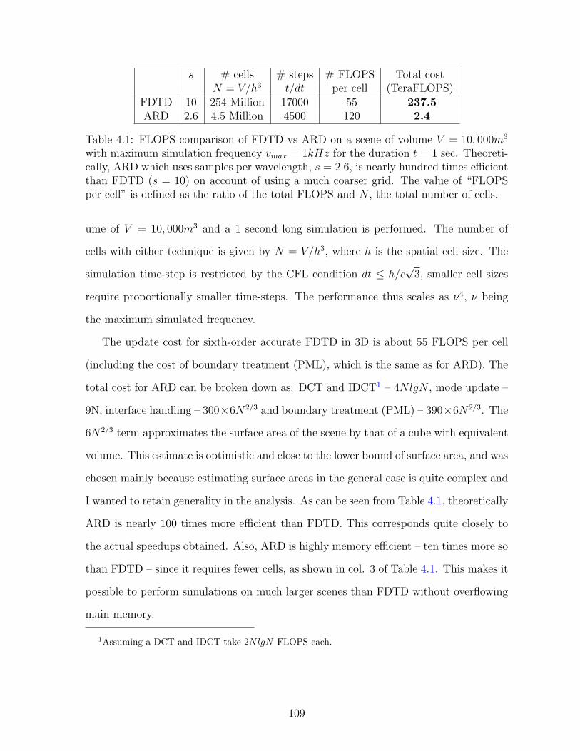
s # cells # steps # FLOPS Total costN = V/h3 t/dt per cell (TeraFLOPS)

FDTD 10 254 Million 17000 55 237.5ARD 2.6 4.5 Million 4500 120 2.4

Table 4.1: FLOPS comparison of FDTD vs ARD on a scene of volume V = 10, 000m3

with maximum simulation frequency vmax = 1kHz for the duration t = 1 sec. Theoreti-cally, ARD which uses samples per wavelength, s = 2.6, is nearly hundred times efficientthan FDTD (s = 10) on account of using a much coarser grid. The value of “FLOPSper cell” is defined as the ratio of the total FLOPS and N , the total number of cells.

ume of V = 10, 000m3 and a 1 second long simulation is performed. The number of

cells with either technique is given by N = V/h3, where h is the spatial cell size. The

simulation time-step is restricted by the CFL condition dt ≤ h/c√3, smaller cell sizes

require proportionally smaller time-steps. The performance thus scales as ν4, ν being

the maximum simulated frequency.

The update cost for sixth-order accurate FDTD in 3D is about 55 FLOPS per cell

(including the cost of boundary treatment (PML), which is the same as for ARD). The

total cost for ARD can be broken down as: DCT and IDCT1 – 4NlgN , mode update –

9N, interface handling – 300×6N2/3 and boundary treatment (PML) – 390×6N2/3. The

6N2/3 term approximates the surface area of the scene by that of a cube with equivalent

volume. This estimate is optimistic and close to the lower bound of surface area, and was

chosen mainly because estimating surface areas in the general case is quite complex and

I wanted to retain generality in the analysis. As can be seen from Table 4.1, theoretically

ARD is nearly 100 times more efficient than FDTD. This corresponds quite closely to

the actual speedups obtained. Also, ARD is highly memory efficient – ten times more so

than FDTD – since it requires fewer cells, as shown in col. 3 of Table 4.1. This makes it

possible to perform simulations on much larger scenes than FDTD without overflowing

main memory.

1Assuming a DCT and IDCT take 2NlgN FLOPS each.

109

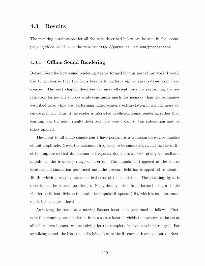
4.3 Results

The resulting auralizations for all the tests described below can be seen in the accom-

panying video, which is at the website: http://gamma.cs.unc.edu/propagation.

4.3.1 Offline Sound Rendering

Before I describe how sound rendering was performed for this part of my work, I would

like to emphasize that the focus here is to perform offline auralizations from fixed

sources. The next chapter describes far more efficient ways for performing the au-

ralization for moving sources while consuming much less memory than the techniques

described here, while also performing high-frequency extrapolation in a much more ac-

curate manner. Thus, if the reader is interested in efficient sound rendering rather than

learning how the audio results described here were obtained, this sub-section may be

safely ignored.

The input to all audio simulations I have perform is a Gaussian-derivative impulse

of unit amplitude. Given the maximum frequency to be simulated, νmax, I fix the width

of the impulse so that its maxima in frequency domain is at νmax

2, giving a broadband

impulse in the frequency range of interest. This impulse is triggered at the source

location and simulation performed until the pressure field has dropped off to about -

40 dB, which is roughly the numerical error of the simulation. The resulting signal is

recorded at the listener position(s). Next, deconvolution is performed using a simple

Fourier coefficient division to obtain the Impulse Response (IR), which is used for sound

rendering at a given location.

Auralizing the sound at a moving listener location is performed as follows. First,

note that running one simulation from a source location yields the pressure variation at

all cell centers because we are solving for the complete field on a volumetric grid. For

auralizing sound, the IRs at all cells lying close to the listener path are computed. Next,

110

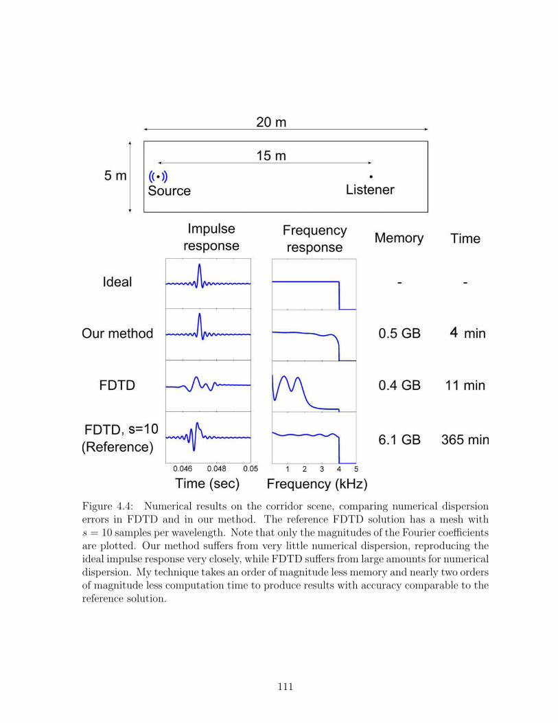
Figure 4.4: Numerical results on the corridor scene, comparing numerical dispersionerrors in FDTD and in our method. The reference FDTD solution has a mesh withs = 10 samples per wavelength. Note that only the magnitudes of the Fourier coefficientsare plotted. Our method suffers from very little numerical dispersion, reproducing theideal impulse response very closely, while FDTD suffers from large amounts for numericaldispersion. My technique takes an order of magnitude less memory and nearly two ordersof magnitude less computation time to produce results with accuracy comparable to thereference solution.

111

Figure 4.5: The House scene demonstrates diffraction of sound around obstacles. All thescene geometry shown was included in the simulation. Our method is able to reproducethe higher diffraction intensity of sound at lower frequencies, while reducing the memoryrequirements by about an order of magnitude and the computational requirements bymore than two orders of magnitude. The reference solution is computed on a mesh withs = 10 samples per wavelength.

the sound at the current position and time is estimated by linearly interpolating the

field values at neighboring cell centers. To obtain the field value at a given cell center, a

convolution of the IR at the corresponding location and the input sound is performed.

Most of the simulations I have performed are band-limited to 1-2kHz due to compu-

tation and memory constraints. However, this is not a big limitation. Although audible

sounds go up to 22kHz, it is important to realize that only frequencies up to about

5kHz are perceptually critical [51] for acoustics simulation. Moreover, the frequency

perception of humans is logarithmic, which reflects in the frequency doubling between

musical octaves. This means that most of the perceptually important frequencies are

contained till about 2kHz. For example, the frequency of the fundamental notes of a

typical 88-key piano goes from about 30Hz to 4kHz, covering 7 octaves, out of which

6 octaves are below 2kHz. However, even though we don’t have accurate perception of

higher frequencies, their complete absence leads to perceptual artifacts and therefore,

there must be some way of accounting for higher frequencies, even if approximately.

One way of doing that would be to combine our technique with a Geometrical Acous-

tic simulator for the higher frequency range. In my work, I have used a much simpler

technique that gives good results in practice.

112

To auralize sounds in the full audible range up to 22kHz, I first up-sample the IR

obtained from the simulation to 44kHz and run a simple peak detector on the IR which

works by searching for local maxima/minima. The resulting IR contains peaks with

varying amplitudes and delays, corresponding to incoming impulses. This is exactly

the kind of IR that geometrical approaches compute by tracing paths for sound and

computing the attenuation and delay along different paths. Each path yields a contri-

bution to the IR. The difference here is that numerical simulation does not explicitly

trace these paths. Instead, my technique extracts this information from the computed

impulse response through peak detection. I use the IR thus computed for higher fre-

quencies. The approximation introduced in this operation is that the diffraction at

higher frequencies is approximated since the peak detector doesn’t differentiate between

reflection and diffraction peaks. Intuitively, this means that high frequencies may also

diffract like low frequencies, which is the approximation introduced by this technique.

This IR filter is then high-passed at the simulation cutoff frequency to yield a filter

to be used exclusively for higher frequencies. As a final step, the exact low-frequency

IR and approximate high-frequency IR are combined in frequency domain to yield the

required IR to be applied on input signals. I must emphasize here that this technique is

applied to obtain an approximate response exclusively in the high-frequency range and

it is ensured that numerical accuracy for lower frequencies till 1-2kHz is maintained.

The reference solution for comparing ARD is the (2,6) FDTD method described in

Section 4.1.2 running on a fine mesh. Since the main bottleneck of our approach is DCT,

which can be performed through an FFT, I used the GPU-based FFT implementation

described in [36], to exploit the compute power available on today’s high-end graphics

cards. Combining optimized transforms with algorithmic improvements described in the

previous sections is the reason my technique gains considerable speedups over FDTD.

All the simulations were performed on a 2.8GHz Intel Xeon CPU, with 8GB of RAM.

The FFTs were performed on an NVIDIA GeForce GTX 280 graphics card.

113

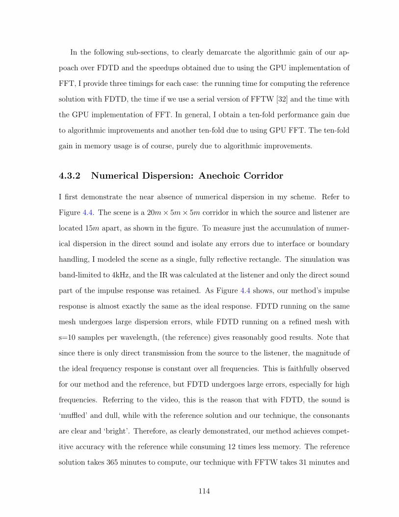
In the following sub-sections, to clearly demarcate the algorithmic gain of our ap-

poach over FDTD and the speedups obtained due to using the GPU implementation of

FFT, I provide three timings for each case: the running time for computing the reference

solution with FDTD, the time if we use a serial version of FFTW [32] and the time with

the GPU implementation of FFT. In general, I obtain a ten-fold performance gain due

to algorithmic improvements and another ten-fold due to using GPU FFT. The ten-fold

gain in memory usage is of course, purely due to algorithmic improvements.

4.3.2 Numerical Dispersion: Anechoic Corridor

I first demonstrate the near absence of numerical dispersion in my scheme. Refer to

Figure 4.4. The scene is a 20m× 5m× 5m corridor in which the source and listener are

located 15m apart, as shown in the figure. To measure just the accumulation of numer-

ical dispersion in the direct sound and isolate any errors due to interface or boundary

handling, I modeled the scene as a single, fully reflective rectangle. The simulation was

band-limited to 4kHz, and the IR was calculated at the listener and only the direct sound

part of the impulse response was retained. As Figure 4.4 shows, our method’s impulse

response is almost exactly the same as the ideal response. FDTD running on the same

mesh undergoes large dispersion errors, while FDTD running on a refined mesh with

s=10 samples per wavelength, (the reference) gives reasonably good results. Note that

since there is only direct transmission from the source to the listener, the magnitude of

the ideal frequency response is constant over all frequencies. This is faithfully observed

for our method and the reference, but FDTD undergoes large errors, especially for high

frequencies. Referring to the video, this is the reason that with FDTD, the sound is

‘muffled’ and dull, while with the reference solution and our technique, the consonants

are clear and ‘bright’. Therefore, as clearly demonstrated, our method achieves compet-

itive accuracy with the reference while consuming 12 times less memory. The reference

solution takes 365 minutes to compute, our technique with FFTW takes 31 minutes and

114

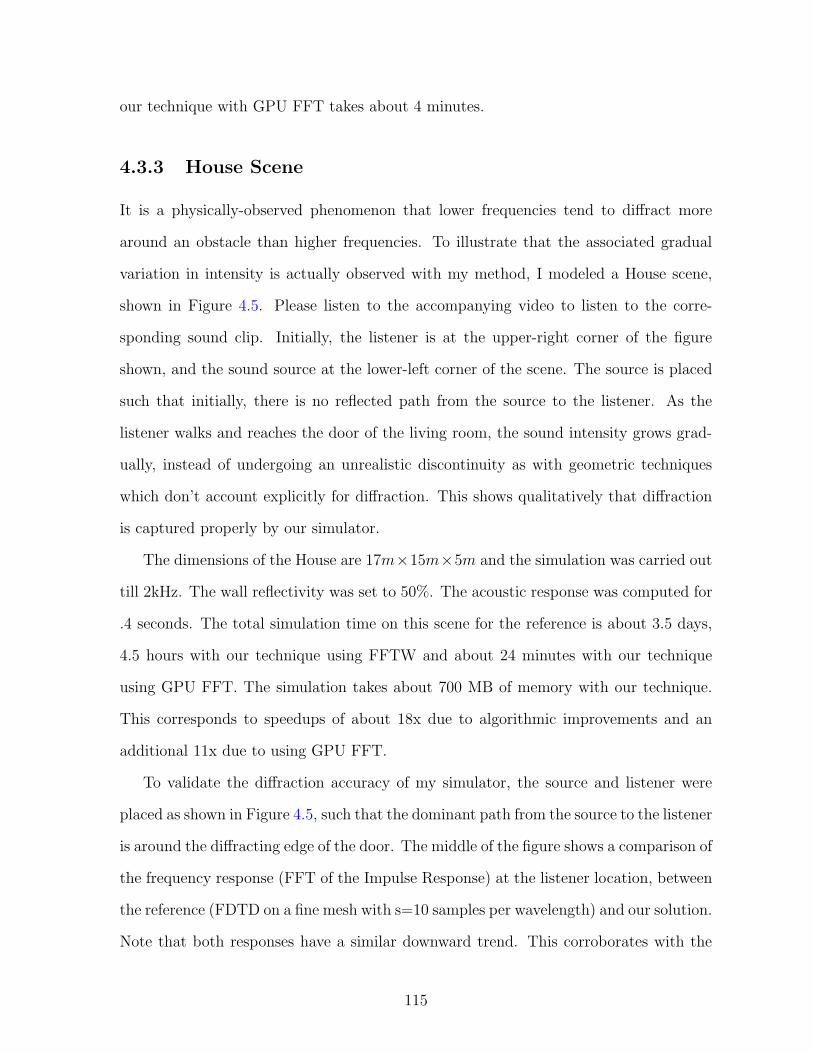
our technique with GPU FFT takes about 4 minutes.

4.3.3 House Scene

It is a physically-observed phenomenon that lower frequencies tend to diffract more

around an obstacle than higher frequencies. To illustrate that the associated gradual

variation in intensity is actually observed with my method, I modeled a House scene,

shown in Figure 4.5. Please listen to the accompanying video to listen to the corre-

sponding sound clip. Initially, the listener is at the upper-right corner of the figure

shown, and the sound source at the lower-left corner of the scene. The source is placed

such that initially, there is no reflected path from the source to the listener. As the

listener walks and reaches the door of the living room, the sound intensity grows grad-

ually, instead of undergoing an unrealistic discontinuity as with geometric techniques

which don’t account explicitly for diffraction. This shows qualitatively that diffraction

is captured properly by our simulator.

The dimensions of the House are 17m×15m×5m and the simulation was carried out

till 2kHz. The wall reflectivity was set to 50%. The acoustic response was computed for

.4 seconds. The total simulation time on this scene for the reference is about 3.5 days,

4.5 hours with our technique using FFTW and about 24 minutes with our technique

using GPU FFT. The simulation takes about 700 MB of memory with our technique.

This corresponds to speedups of about 18x due to algorithmic improvements and an

additional 11x due to using GPU FFT.

To validate the diffraction accuracy of my simulator, the source and listener were

placed as shown in Figure 4.5, such that the dominant path from the source to the listener

is around the diffracting edge of the door. The middle of the figure shows a comparison of

the frequency response (FFT of the Impulse Response) at the listener location, between

the reference (FDTD on a fine mesh with s=10 samples per wavelength) and our solution.

Note that both responses have a similar downward trend. This corroborates with the

115

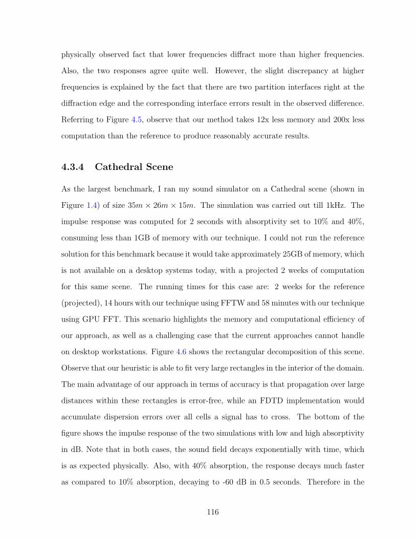
physically observed fact that lower frequencies diffract more than higher frequencies.

Also, the two responses agree quite well. However, the slight discrepancy at higher

frequencies is explained by the fact that there are two partition interfaces right at the

diffraction edge and the corresponding interface errors result in the observed difference.

Referring to Figure 4.5, observe that our method takes 12x less memory and 200x less

computation than the reference to produce reasonably accurate results.

4.3.4 Cathedral Scene

As the largest benchmark, I ran my sound simulator on a Cathedral scene (shown in

Figure 1.4) of size 35m × 26m × 15m. The simulation was carried out till 1kHz. The

impulse response was computed for 2 seconds with absorptivity set to 10% and 40%,

consuming less than 1GB of memory with our technique. I could not run the reference

solution for this benchmark because it would take approximately 25GB of memory, which

is not available on a desktop systems today, with a projected 2 weeks of computation

for this same scene. The running times for this case are: 2 weeks for the reference

(projected), 14 hours with our technique using FFTW and 58 minutes with our technique

using GPU FFT. This scenario highlights the memory and computational efficiency of

our approach, as well as a challenging case that the current approaches cannot handle

on desktop workstations. Figure 4.6 shows the rectangular decomposition of this scene.

Observe that our heuristic is able to fit very large rectangles in the interior of the domain.

The main advantage of our approach in terms of accuracy is that propagation over large

distances within these rectangles is error-free, while an FDTD implementation would

accumulate dispersion errors over all cells a signal has to cross. The bottom of the

figure shows the impulse response of the two simulations with low and high absorptivity

in dB. Note that in both cases, the sound field decays exponentially with time, which

is as expected physically. Also, with 40% absorption, the response decays much faster

as compared to 10% absorption, decaying to -60 dB in 0.5 seconds. Therefore in the

116

corresponding video, with low absorption, the sound is less coherent and individual

notes are hard to discern, because strong reverberations from the walls interfere with

the direct sound. This is similar to what is observed in cathedrals in reality.

Also note that my technique is able to capture high order reflections, corresponding

to about 30 reflections in this scene. This late reverberation phase captures the echoic

trail-off of sound in an environment. Geometric techniques typically have considerable

degradation in performance with the order of reflections and are therefore usually limited

to a few reflections. My technique is able to capture such high order reflections because

of two reasons: Firstly, because it is a numerical solver which works directly with the

volumetric sound field and is thus insensitive to the number of reflections. Secondly,

as discussed in Section 4.3.2, our technique has very low numerical dispersion and thus

preserves the signal well over long distances. For 30 reflections in the Cathedral, the

signal must travel about 600 meters without much dispersion. As discussed earlier, with

FDTD running on the same mesh, the signal would be destroyed in about 20 meters.

4.4 Conclusion and Future Work

I have presented a computation- and memory-efficient technique (ARD) for performing

accurate numerical acoustic simulations on complex domains with millions of cells, for

sounds in the kHz range. My method exploits the analytical solution to the Wave Equa-

tion in rectangular domains and is at least an order of magnitude more efficient, both in

terms of memory and computation, compared to a reference (2,6) FDTD scheme. Con-

sequently, my technique is able to perform physically accurate sound simulation, which

yields perceptually convincing results containing physical effects such as diffraction. My

technique is capable of performing numerical sound simulations on large, complex 3D

scenes, which, to the best of our knowledge, was not previously possible on a desktop

computer.

117

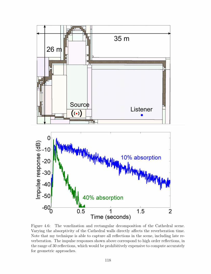
Figure 4.6: The voxelization and rectangular decomposition of the Cathedral scene.Varying the absorptivity of the Cathedral walls directly affects the reverberation time.Note that my technique is able to capture all reflections in the scene, including late re-verberation. The impulse responses shown above correspond to high order reflections, inthe range of 30 reflections, which would be prohibitively expensive to compute accuratelyfor geometric approaches.

118

One of the areas where this implementation may be improved is to add a fine-grid

simulation, possibly based on FDTD, near the boundary to reduce boundary reflec-

tion errors. Another important improvement would be the addition of support for

frequency-dependent absorption at the scene boundary, which is quite important acous-

tically. It might be possible to address both these problems at once by utilizing the

recent work by Savioja et. al. [90]. This technique uses the interpolated wideband

FDTD (IWB-FDTD) scheme [49] to control numerical dispersion. It is shown that dig-

ital impedance filters [49] can be integrated with this technique, making it capable of

handling frequency-dependent absorption. Thus, one can imagine ARD running strictly

in the interior of the domain on a coarse grid, while the IWB-FDTD technique is used

on a fine grid near the boundary. Such an integration would retain computational ef-

ficiency, since the fine grid is confined to a region proportional to the surface area of

the scene, while resulting in simulations with much more accurate boundary treatment

– the finer grid would ensure reduced stair-casing errors and digital impedance filters

would capture frequency-dependent reflections.

For the foreseeable future it seems that even after the increase in computational and

memory efficiency with the ARD approach, numerical approaches will not be feasible

for large 3D scenes for the full audible range till 22kHz. It is interesting to note in this

context that geometric and numerical approaches are complimentary with regard to the

range of frequencies they can simulate efficiently – with geometric approaches it is hard

to simulate low-frequency wave phenomena like diffraction because they assume that

sound travels in straight lines like light, while with numerical approaches, simulating

high frequencies above a few kilohertz becomes prohibitive due to the excessively fine

volume mesh that must be created. Thus, a hybridization of the two techniques, once

numerical techniques can be stretched to work till roughly 4kHz, seems like the best

alternative. Above 4kHz, diffraction won’t be a concern for most scenes and ray-tracing

based geometric techniques would work very well. This goal of 4kHz for numerical

119

approaches seems to be in reach within a few years for scenes with dimensions similar to

typical concert halls. ARD is already capable of working till about 1kHz on such scenes.

For handling sounds till 4kHz, (4kHz/1kHz)4 = 256 times the computation is needed.

This can be achieved by a combination of improving ARD’s numerical characteristics to

work for even coarser meshes. However, this would offer limited advantage because ARD

already operates quite close to the Nyquist limit. Another promising direction would be

by exploiting the computational power of Graphics Processing Units (GPUs) and move

all stages of the ARD pipeline to GPUs. I am currently part of such an exploration and

promising speedups of nearly ten times have already been reported [57].

120

Chapter 5

Interactive Sound Propagation

The previous chapter focused on an efficient technique I have developed to perform

band-limited wave-based acoustic simulations on realistic spaces. The amount of data

generated by a typical numerical simulation is very large, typically ranging in tens of

gigabytes, for simulation from a single source location. Allowing for moving sources re-

quires sampling from hundreds or thousands such source locations, which clearly makes

the memory requirements intractable. The aim of this chapter is to describe a technique

and associated system I have developed that can use these numerical simulations as a

pre-processing step to allow interactive auralizations with moving sources and listener in

an arbitrary 3D environment. This capability requires efficient techniques that exploit

human auditory perception such that the runtime memory usage and performance are

affordable for interactive applications. Also, it also achieves the desirable goal that the

pre-processing time is usually limited to a few hours on today’s desktop systems, which

could otherwise range into days with standard finite-difference time-domain techniques.

The chapter is organized as follows: First I discuss the perceptual properties of reverber-

ant spaces. This is intricately related to research in the area of room acoustics which is

a vast area in itself. My focus is only on the parts that are directly relevant to my work.

In Section 5.2, I give a detailed description of my technique that extensively uses these

perceptual observations to post-process and store the results of numerical simulations

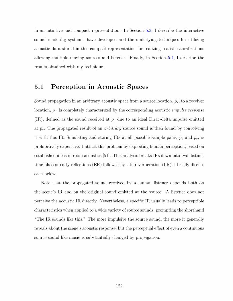
in an intuitive and compact representation. In Section 5.3, I describe the interactive

sound rendering system I have developed and the underlying techniques for utilizing

acoustic data stored in this compact representation for realizing realistic auralizations

allowing multiple moving sources and listener. Finally, in Section 5.4, I describe the

results obtained with my technique.

5.1 Perception in Acoustic Spaces

Sound propagation in an arbitrary acoustic space from a source location, ps, to a receiver

location, pr, is completely characterized by the corresponding acoustic impulse response

(IR), defined as the sound received at pr due to an ideal Dirac-delta impulse emitted

at ps. The propagated result of an arbitrary source sound is then found by convolving

it with this IR. Simulating and storing IRs at all possible sample pairs, ps and pr, is

prohibitively expensive. I attack this problem by exploiting human perception, based on

established ideas in room acoustics [51]. This analysis breaks IRs down into two distinct

time phases: early reflections (ER) followed by late reverberation (LR). I briefly discuss

each below.

Note that the propagated sound received by a human listener depends both on

the scene’s IR and on the original sound emitted at the source. A listener does not

perceive the acoustic IR directly. Nevertheless, a specific IR usually leads to perceptible

characteristics when applied to a wide variety of source sounds, prompting the shorthand

“The IR sounds like this.” The more impulsive the source sound, the more it generally

reveals about the scene’s acoustic response, but the perceptual effect of even a continuous

source sound like music is substantially changed by propagation.

122

time

Impulse Response

direct

reflected

frequency (Hz)

Frequency Response

0

1

a

1+a

1-a

∆t 1/∆t

Figure 5.1: Impulse response (IR) and corresponding frequency response (FR)for a simple scene with one reflection.

5.1.1 Early Reflections (ER)

The ER phase is characterized by a sparse set of high-amplitude pressure peaks, and

captures position-dependent variation in loudness, spectral coloration and echoes. Con-

sider the scene shown in Figure 5.1. The scene’s propagated response can be examined

in two ways: in the time domain, as the impulse response shown on the bottom-left in

Figure 5.1, and equivalently, in the frequency domain, as the complex frequency response

(FR) whose magnitude is shown on the bottom-right. The IR is a set of two impulse

peaks, separated in time by Δt. Assuming the amplitudes of the peaks to be 1 and a,

the FR is a comb-filter that oscillates between 1 + a and 1 − a with “between-teeth”

bandwidth of 1/Δt.

When Δt is above 60-70ms, known as the “echo threshold” [53], we perceive a distinct

echo, especially for impulsive sources. If the delay is much smaller, the peaks fuse in our

perception resulting in no distinct echo. However, the corresponding FR’s between-teeth

bandwidth, which is equal to 1/Δt, increases as Δt is reduced, and our auditory system is

able to extract the resulting selective attenuation of frequencies. The result is perceived

as a comb-filtered, “colored” sound. The most dramatic example this phenomenon of

123

coloration is in small spaces with smooth reflective surfaces, such as an office corridor

or shower.

Following [51, p. 203], if the delay is larger than 20-25ms (FR between-teeth band-

width less than 50Hz), coloration becomes inaudible due to our auditory system’s limited

frequency discrimination [40]. I thus assume that errors in peak delays and amplitudes

are tolerable as long as they preserve FR features up to a resolution of 50Hz. Between

these thresholds (25ms-60ms), our perception transitions from coloration to echoes, lead-

ing to “rough” sounds.

ERs in real scenes are determined by numerous interactions with the boundary. In

an empty room, the ER has low temporal density and audible coloration. In a furnished

room, sound is scattered more highly, yielding an ER with dense, smaller peaks and

leading to a warmer sound. The ER also depends on occlusion, as the sound field

diffracts around obstacles leading to spatial variation in its loudness and frequency

response.

5.1.2 Late Reverberation (LR)

After undergoing many boundary interactions, the sound field enters the LR phase,

becoming dense and chaotic in time and space. The LR between any source and receiver

consists of numerous small-amplitude peaks. These peaks are not individually perceived,

only their overall decay envelope, which causes reverberations to fade out over time. The

decay curve stays largely constant within a room [51, p. 209] and depends on its global

geometry.

An important feature of my approach is that it directly simulates the LR, and so

captures its decay curve automatically from scene geometry. This is possible because

numerical simulation scales linearly in simulated time duration and is insensitive to the

order of boundary interactions. Computing the LR from scene geometry also ensures

that the ER and LR match, preserving realism. The LR is characterized by peak density:

124

1000 peaks per second indicate a fully-developed LR phase [34]. I use a value of 500

peaks per second as the LR’s onset.

5.2 Acoustic Precomputation

The precomputation begins by running an LR probe simulation, which places a source

at the centroid of each room in the scene as described in Section 5.2.2. These LR

simulations determine the time at which the ER phase transitions to the LR phase,

denoted TER. TER depends on the room size. Larger spaces require more time for

the sound field to become stochastic; i.e., to reach the required peak density. This is

detected automatically by processing on the LR probe data and taking the maximum

over all rooms in the scene. For the scenes I have experimented with, values of 50-200ms

are obtained.

In many applications, the listener’s position is more constrained than the sources’.

This can be exploited to reduce memory and preprocessing time. Uniform samples

are placed over a region representing possible locations of the listener at runtime, but

are considered as sources in the precomputed simulation. The principle of acoustic

reciprocity means that we can reverse the simulated sense of source and listener at run-

time. Simulations are then run over multiple source positions, ps, for time length TER, to

record the spatially-varying ER impulse response (ERIR). For each source, the resulting

time-varying field is recorded at samples, pr, uniformly distributed over the entire 3D

scene volume. Each source and receiver sample generates a time-varying sound signal,

s(t), which is then processed as described in Section 5.2.3 to extract its relevant content

and yield a compact result.

125

5.2.1 Numerical Simulation

I utilize the ARD numerical acoustic simulator I have developed. It is fast yet still able to

propagate an input signal over long distances and many reflections without distorting the

waveform due to numerical dispersion errors that arise in finite difference approaches.

This is crucial in subsequent processing – dispersion introduces artificial ringing and

leads to the detection of spurious peaks during the peak detection phase, which I will

describe later. Such spurious peaks would be interpreted as separate physical reflections,

generating errors in the final auralization.

Input to the simulator is the room geometry, absorption parameters (potentially

varying per surface triangle), grid resolution, source reference signal, and source loca-

tion. The simulator then generates the resulting sound at each time-step and at all grid

cell centers in 3D. A single run of the simulator thus captures the whole room’s acoustic

response at every possible listener location, from a fixed source location. Currently,

my simulator models spatially-varying but not frequency-dependent sound absorption.

Including frequency-dependent absorption requires modifications to the ARD simula-

tor, as discussed in Section 4.4 and would lead to more realistic auralizations, without

affecting the approach presented here.

The reference input signal propagated from the source location is a Gaussian pulse

of unit amplitude, given by:

G (t) = exp

(−(t− 5σ)2

σ2

), (5.1)

where σ = (πηf )−1 and ηf is the simulation’s frequency limit, typically 1000Hz. This

function’s Fourier transform is a broadband Gaussian spanning all frequencies from 0

to ηf .

126

Bandlimited simulation To keep preprocessing time and storage manageable, the

simulation frequencies are limited up to ηf . A practical limit used in most of the exam-

ples is ηf = 1000Hz, with a corresponding grid resolution of about 10cm. Information

at higher frequencies must be extrapolated. This limitation of the precomputation be-

comes less of a problem as computational power increases; the run-time supports the

results of higher-frequency simulation without change or additional cost. Frequencies in

the range 100Hz to 5000Hz are most important perceptually for room acoustics [51, p.

27]. Though humans can hear higher frequencies, they quickly attenuate in air and are

highly absorbed by most surfaces.

The simulation’s frequency gap between 1kHz and 5kHz yields two major types of

error. First, it limits the time resolution at which peaks can be separated to 500μs.

Merging a high-amplitude peak with another, which follows closer than this limit elimi-

nates coloration effects. The auralizations thus neglect some high-frequency coloration.

Second, diffraction information is unavailable beyond 1kHz. My method for extrapolat-

ing the frequency trend in Section 5.2.3 produces a plausible, natural-sounding result in

this gap.

Spatial sampling The spatial accuracy at which we perceive sound fields is limited.

A human head acts as a diffractive occluder which destroys interference patterns at

smaller spatial resolution. I thus speculate that its size (�10cm) is a guide to the

smallest sampling resolution required for convincing auralization in typical scenes. To

my knowledge the question is an open research problem.

My simulator generates spatial samples for the receiver near this resolution, but I

further downsample them by a factor of 8× in each dimension to reduce run-time memory

requirements. Typical receiver grid resolution is about 1m. Using the interpolation

method proposed in the next section, subsampled IRs still provide perceptually artifact-

free results without clicks or gurgling, as demonstrated in the accompanying video (link

127

given in Section 5.4). The sound field changes convincingly as the sources and listener

move around obstructions. Increasing spatial resolution would use more memory but

would not significantly affect runtime performance, since the expense is dominated by

FFTs rather than spatial interpolation.

5.2.2 LR Processing

The purpose of the LR probe simulation is to compute the duration of the ER phase,

TER, and the LRIR. A peak detector is run on the simulated probe response to generate

a set of peak delay/amplitude data, {ti, ai}, sorted on delays, ti. This is shown in the

upper right of Figure 5.2. Simulations bandlimited to 1kHz imply a quantization of

peak delays at roughly 500μs. Such quantization can introduce artificial periodicities

and lead to audible but false coloration. The peak times are perturbed by a random

value in the range -500 to +500 μs. Any periodicities above a few milliseconds, including

“fluttering” effects in the LR, are still preserved.

Peak detection A straightforward algorithm is used to for peak detection in my

technique. It scans the time-dependent signal for maxima and minima by comparing

each value with both its neighbors. Detected signal extrema are recorded in terms

of their time and amplitude. Such a simple detector is sensitive to noise and would

be inappropriate for physically-measured IRs. It works well however on the results of

noise-free bandlimited simulations.

LR duration After peak detection, the LR is conservatively truncated when it has

decayed by 90dB. The resulting duration, TLR, is calculated as follows. First, the signal’s

decay envelope, d(t), is constructed from the peaks detected previously via

d(t) = 10× log(ai2), ti ≤ t < ti+1 (5.2)

128

This operation converts pressure amplitudes to intensities and fills out spaces between

peaks. Then, smoothing in time is performed by applying a moving average filter on

d(t) of width 40ms. TLR is given by the smallest t such that d(0) − d(t) > 90. Peaks

with delays beyond TLR are then removed.

ER duration As explained in Section 5.1, TER is calculated as the time when peak

density reaches 500 peaks per second. Starting from time t = 0, all peaks within the

range [t, t + 20ms] are considered and only those are counted that are within 20 dB of

the highest intensity peak in the interval. If the number of such peaks exceeds 500 per

second × 0.02 seconds = 10 peaks, this t is recorded as the ER duration. Otherwise,

t is increased by 20ms and this is continued until the criterion is satisfied. Since peak

density increases with time, this procedure terminates.

Increasing LR peak density Because the simulator is frequency band-limited, it can

detect no more than 1000 peaks per second. While this is sufficient for music and voice, it

is not for impulsive sources such as gunshots or footsteps, which require roughly 10,000

peaks per second [34]. Following practice in artificial reverberators, peaks are added

stochastically to increase the density by a factor of 10. This is done while preserving

the decay envelope, as follows.

First, a densification factor, F (t), TER ≤ t < TLR is computed as

F (t) = 10

(t− TER

TLR − TER

)2

. (5.3)

F(t) builds quadratically in time from 0 to a terminal value of 10, based on the expected

quadratic growth in peak density in physical scenes [51, p. 98]. Next, for each peak

{ti, ai} in the LR after time TER, �F (ti) additional peaks are added with amplitudes

ai× rand(−1, 1). This preserves the simulated decay envelope and yields the final LRIR

for use at runtime.

129

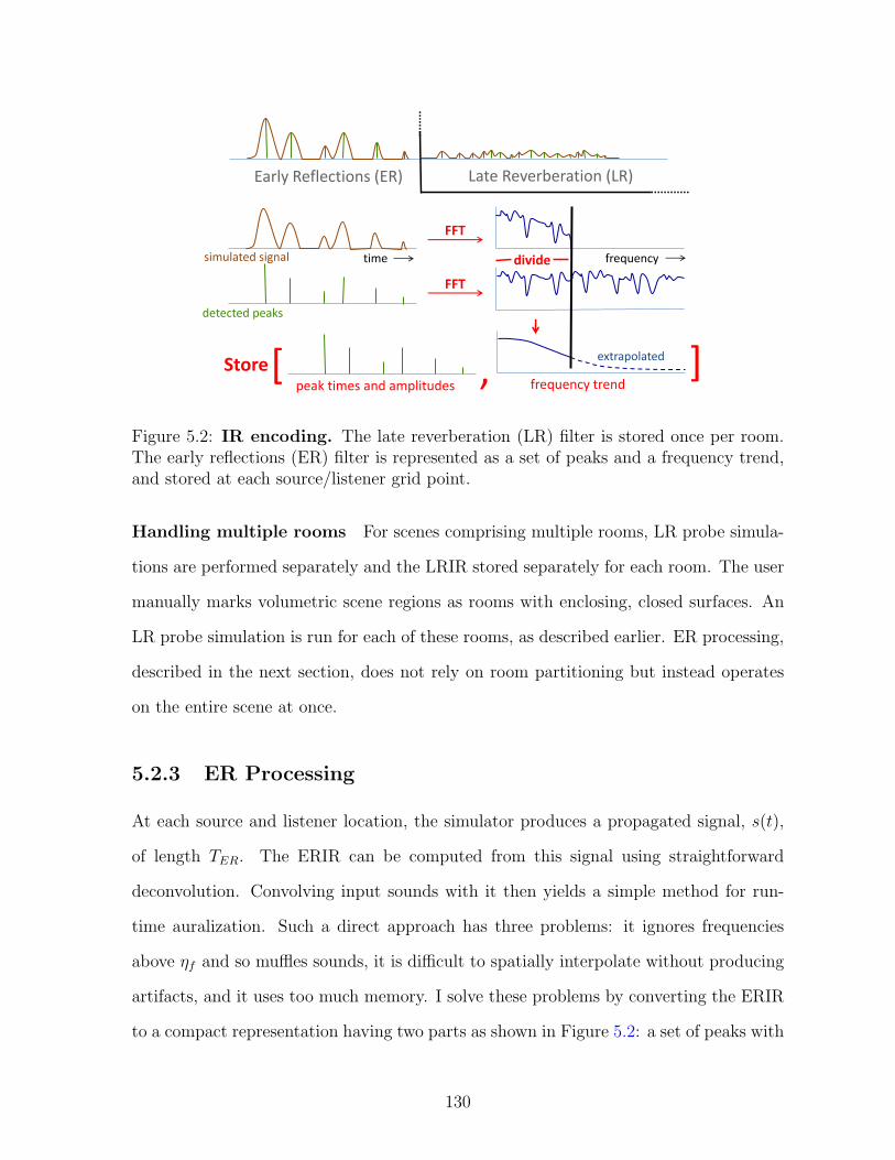
Early Reflections (ER) Late Reverberation (LR)

FFT

FFT

dividetime

Store ,[ ]peak times and amplitudes frequency trend

extrapolated

frequencysimulated signal

detected peaks

Figure 5.2: IR encoding. The late reverberation (LR) filter is stored once per room.The early reflections (ER) filter is represented as a set of peaks and a frequency trend,and stored at each source/listener grid point.

Handling multiple rooms For scenes comprising multiple rooms, LR probe simula-

tions are performed separately and the LRIR stored separately for each room. The user

manually marks volumetric scene regions as rooms with enclosing, closed surfaces. An

LR probe simulation is run for each of these rooms, as described earlier. ER processing,

described in the next section, does not rely on room partitioning but instead operates

on the entire scene at once.

5.2.3 ER Processing

At each source and listener location, the simulator produces a propagated signal, s(t),

of length TER. The ERIR can be computed from this signal using straightforward

deconvolution. Convolving input sounds with it then yields a simple method for run-

time auralization. Such a direct approach has three problems: it ignores frequencies

above ηf and so muffles sounds, it is difficult to spatially interpolate without producing

artifacts, and it uses too much memory. I solve these problems by converting the ERIR

to a compact representation having two parts as shown in Figure 5.2: a set of peaks with

130

associated delays and amplitudes, and a residual frequency response magnitude, called

the frequency trend. ER peaks capture the main time-domain information such as high-

amplitude reflections, as well as coloration effects as described in Section 5.1.1, while

the frequency trend accounts for residual frequency-dependent attenuation including

low-pass filtering due to diffraction.

Peak information is naturally all-frequency, and so applies to arbitrary inputs without

muffling. Only the frequency trend needs to be extrapolated to higher-frequency input

signals.

Peak Extraction

A simple method for detecting peaks in the recorded response, s(t), is to run the peak

detector introduced in Section 5.2.2. Let’s denote this set of peaks as P . First, low-

amplitude peaks from P are removed using a threshold of 40dB below the highest-

amplitude peak present. Such peaks are masked by the higher energy peaks.

Unfortunately, this method merges peaks separated by less than 1ms, since sums

of closely-separated Gaussians have only one extremal point. This can be improved:

using results from a simulation bandlimited to 1kHz, it is possible in theory to resolve

peaks separated by as little as 0.5ms. The following describes an approach that extracts

more information from the simulation in order to preserve coloration effects and simplify

later processing to extract the frequency trend. It doesn’t guarantee all theoretically-

resolvable peaks are detected but provides good results in practice.

The ideal impulse response, I(t), is computed by performing a deconvolution on s(t)

with the input signal G(t) given in (5.1). Using ⊗ to denote convolution, � to denote

element-wise complex multiplication, and x to denote the Fourier transform of x, the

convolution theorem states that

s(t) = G(t)⊗ I(t) ⇔ s(f) = G(f)� I(f). (5.4)

131

To solve for the IR I given s and G, deconvolution is performed using a frequency

coefficient complex division to obtain

I(f) =s(f)

G(f). (5.5)

An inverse FFT on I(f) then yields I(t). Before performing it though, I must be low-

pass filtered to eliminate frequencies above ηf , since these are outside the simulator’s

range and contain large numerical errors.1 This can be done by zero-padding the FR

vector above ηf up to the target rate of 44.1kHz. It is well-known that such an abrupt

zeroing or “brick-wall filtering” leads to ringing artifacts in the time domain and so

to fictitious peaks. At the same time, it provides the best possible time resolution for

separating peaks.

The problem then is to generate a set of super-resolved peaks P ′ from I(t) that are

guaranteed to be real and not “rings” of earlier peaks, in order to separate high-energy

peaks to the fullest possible extent and preserve their audible coloration.

Finding super-resolved peaks P ′ A bound on ringing error in I(t) can be computed

by observing that brick-wall filtering turns an ideal peak into a Sinc function, having

a 1/t time-decaying amplitude. An error envelope, e(t), can therefore be built against

which later peaks in I(t) can be culled to account for “rings” of earlier ones. P ′ is

initialized to contain all peaks detected from the ideal IR, I(t), including rings. Only

peaks within 20dB of the highest amplitude one are retained, since we are interested in

closely-spaced, high-amplitude peaks that create strong oscillations in the FR.

A ringing envelope, S(t), is then defined as the low-pass filtering result of a unit

1The reader might wonder why such low-pass filtering was not also applied to the signal s(t) beforeperforming peak detection on it. The reason is that the input source signal G(t) and its response s(t)contain little energy above ηf . It is only when frequency-domain values are divided by each otherduring deconvolution that a non-negligible result is obtained at higher frequencies, requiring cleanup.

132

ideal impulse at t = 0 to a frequency limit of ηf :

S(t) =

⎧⎪⎪⎪⎪⎨⎪⎪⎪⎪⎩0, |t| < t0

|sin(ωt)| /ωt, t0 ≤ |t| < t1

1/ωt, |t| ≥ t1

(5.6)

where t0 = 0.5/ηf , t1 = 0.75/ηf , and ω = 2πηf . The time t0 represents the first zero

of the Sinc while t1 represents the following minimum of its negative side lobe. The

envelope thus bounds ringing that occurs after a peak’s main lobe. If an ideal peak is

band-passed, peak detection run on it, and all peaks with absolute amplitudes less than

this envelope culled, only the original peak remains.

To build the complete error envelope, e(t), we accumulate these over each peak in

P ′ = {ai, ti} via

e(t) =∑i

|ai|S(t− ti) (5.7)

The fact that P ′ itself contains ringing peaks serves to make the envelope conservative

in the sense that in the worst case we may remove a real peak but never fail to remove

a ringing peak. Culling is straightforward: a peak (ai, ti) is removed if |ai| < e(ti).

Supplementing P with P ′ I use P ′ to supplement P since multiple peaks in P ′ may

have merged to a single peak in P . This is done by scanning through all peaks in P ′ and

assigning each to the peak in P closest to it in time. Then, each peak in P is replaced

with the set of peaks in P ′ that were assigned to it, yielding the final set of peaks. This

automatic procedure generates about N=20-50 peaks in all the scenes I have tested.

Frequency Trend Extraction

Peak extraction ignores diffraction and implicitly assumes every peak acts on all fre-

quencies uniformly. Diffraction introduces frequency-dependent filtering not captured

by this set of peaks. This residual information is captured by my method of frequency

133

trend extraction, as illustrated in the middle of Figure 5.2. It compares the simulated

FR, I(f), to the FR of the idealized IR composed of the extracted peaks, P , in order to

extract any residual low-pass trend due to diffraction. The following description assumes

ηf=1kHz, the typical frequency limit in this work.

The impulse response corresponding to the extracted ER peaks, I ′, is constructed

by summing over its peaks via

I ′ =N∑i=1

ai δ(t− ti) (5.8)

where δ(t) is the discrete analog of the Dirac-delta function – a unit-amplitude pulse of

one sample width. Its corresponding FR is denoted I ′. The FR of the ideal IR of the

original simulation, I, is also constructed, which contains complete information up to

frequencies of 1kHz. The overall frequency-dependent diffraction trend for f ≤ 1kHz is

obtained via

T (f) =

∣∣∣I(f)∣∣∣∣∣∣I ′(f)∣∣∣ . (5.9)

Before performing this division, both the numerator and denominator are smoothed

with a Gaussian of width 50Hz. The unsmoothed I ′(f) often has near-zero values;

smoothing takes care of this problem and makes the above operation numerically stable.

As explained in Section 5.1.1, this has little perceptual impact because we are insensitive

to finer details in the magnitude frequency response. T (f) is then smoothed again with

the same Gaussian to yield the final frequency trend. Average values of T (f) in each

octave band 0-62.5Hz, 62.5-125Hz, . . ., 500-1000Hz are then stored.

This trend contains information only up to 1kHz. Fortunately, much of the per-

ceivable diffraction-related occlusion effect in common acoustic spaces manifests itself

in frequencies below 1kHz [51]. Sound wavelength for 1kHz is about 34cm, which is

comparable to large features such as pillars, doors and windows.

This trend can be plausibly extrapolated to frequencies higher than were simulated.

134

To do this, T (f) is expressed on a log-log scale, which corresponds to plotting the power

at each frequency, in dB, against the frequencies in octaves. These scales better match

our loudness and pitch perception. Moreover, the low-pass diffraction trend for physical

edges is roughly linear on such a log-log scale for mid-to-high frequencies [98]. A line is

then fit to the log-log trend in the frequency range 125-1000Hz. If the slope is negative,

indicating a low-pass trend, the line is extrapolated and stored at octave bands higher

than 1000Hz up to 22,050Hz. If the slope is positive, extrapolation is not performed;

instead the value at the 500-1000Hz octave is just copied into to higher ones.

5.3 Interactive Auralization Runtime

The precomputed, perceptually-encoded information from numerical simulation sup-

ports interactive sound propagation from moving sources to a moving listener. My

approach performs perceptually-smooth spatial interpolation of the IRs, and then prop-

agates source sounds by convolving them with these IRs. My technique generates re-

alistically dense IRs, and the run-time works in the frequency domain to perform the

convolution efficiently. A schematic diagram of my real-time auralization system is

shown in Figure 5.3.

5.3.1 Load-time Computation

At load-time, per-room LR filters are loaded and processed. The initial TER part of the

LRIR is zeroed out, to be replaced at run-time with the spatially-varying ERIR. The

LRIR’s Fourier Transform ILR is then computed and stored, along with its time-domain

peaks.

Next, ERIR filters for the whole scene are loaded, yielding a table, IER(ps, pr), where

points ps lie on a 2.5D region of potential listener positions and pr sample sources over

the entire 3D volume of the scene. Note the reversal of sense of source/listener from

135

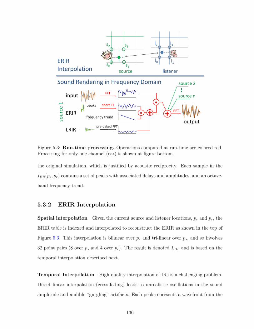
ERIR Interpolation

Sound Rendering in Frequency Domain

source listeners0 s1

s2 s3

l0 l1

l2 l3

.+ IFFT

FFT

output

source 2

source n

short FT

pre-baked FFT

input

ERIR

LRIR

frequency trend. +

sour

ce 1 peaks

Figure 5.3: Run-time processing. Operations computed at run-time are colored red.Processing for only one channel (ear) is shown at figure bottom.

the original simulation, which is justified by acoustic reciprocity. Each sample in the

IER(ps, pr) contains a set of peaks with associated delays and amplitudes, and an octave-

band frequency trend.

5.3.2 ERIR Interpolation

Spatial interpolation Given the current source and listener locations, ps and pr, the

ERIR table is indexed and interpolated to reconstruct the ERIR as shown in the top of

Figure 5.3. This interpolation is bilinear over pr and tri-linear over ps, and so involves

32 point pairs (8 over ps and 4 over pr). The result is denoted ISL, and is based on the

temporal interpolation described next.

Temporal Interpolation High-quality interpolation of IRs is a challenging problem.

Direct linear interpolation (cross-fading) leads to unrealistic oscillations in the sound

amplitude and audible “gurgling” artifacts. Each peak represents a wavefront from the

136

source arriving at the listener. As the listener moves, this peak smoothly translates

in time; cross-fading instead generates twin “ghosts” which only modify amplitudes at

fixed peak times evaluated at the two spatial samples. Frequency-domain interpolation

fails to help because the time and frequency domains are linearly related. Interpolating

over the peak delays and amplitudes that are extracted in my technique better matches

the physical situation and produces no artifacts in all the experiments performed.

Interpolating between delays and amplitudes of two peaks assumes that they corre-

spond; i.e., belong to the same propagating wavefront. The finite speed of sound dictates

that the peaks from the same wavefront at two points in space separated by a distance

Δd can be separated in time by no more than

Δt ≤ Δd

c, (5.10)

where Δd is the spatial sampling distance (1m) and c is the speed of sound in air, 343m/s

at 20◦C. The following procedure computes correspondences and achieves convincing

interpolation.

Denote the peak sets of the two IRs as P1 and P2, and assume both are sorted

over peak times ti. Construct a graph whose edges represent potential correspondence

between a peak in P1 and a peak in P2; in other words, the difference between peak

times satisfies (5.10). Edge weight is assigned the absolute value of the peaks’ amplitude

difference. The algorithm iterates greedily by selecting the edge of smallest weight

currently in the set, finalizing it as a correspondence, and removing all other edges

sharing either of the two peaks selected. The operation is commutative in P1 and P2

and interpolates associated peak delays and amplitudes, yielding a perceptually smooth

auralization for moving sources and listener.

In addition to peaks, the ERIR’s frequency trend must also be interpolated. In this

case, straightforward linear interpolation of amplitudes in each octave band works well.

137

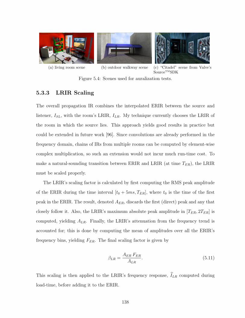
(a) living room scene (b) outdoor walkway scene (c) “Citadel” scene from Valve’sSourceTMSDK

Figure 5.4: Scenes used for auralization tests.

5.3.3 LRIR Scaling

The overall propagation IR combines the interpolated ERIR between the source and

listener, ISL, with the room’s LRIR, ILR. My technique currently chooses the LRIR of

the room in which the source lies. This approach yields good results in practice but

could be extended in future work [96]. Since convolutions are already performed in the

frequency domain, chains of IRs from multiple rooms can be computed by element-wise

complex multiplication, so such an extension would not incur much run-time cost. To

make a natural-sounding transition between ERIR and LRIR (at time TER), the LRIR

must be scaled properly.

The LRIR’s scaling factor is calculated by first computing the RMS peak amplitude

of the ERIR during the time interval [t0 + 5ms, TER], where t0 is the time of the first

peak in the ERIR. The result, denoted AER, discards the first (direct) peak and any that

closely follow it. Also, the LRIR’s maximum absolute peak amplitude in [TER, 2TER] is

computed, yielding ALR. Finally, the LRIR’s attenuation from the frequency trend is

accounted for; this is done by computing the mean of amplitudes over all the ERIR’s

frequency bins, yielding FER. The final scaling factor is given by

βLR =AER FER

ALR

. (5.11)

This scaling is then applied to the LRIR’s frequency response, ILR computed during

load-time, before adding it to the ERIR.

138

5.3.4 Binaural Processing

Human auditory perception is binaural; that is, based on two ears. This allows us

to estimate direction and distance to sound sources, a capability known as localization

[10]. Ideally, this requires augmenting each peak in the ERIR with information about the

corresponding wavefront gradient; i.e., the direction in which the sound is propagating.

It may be possible to extract such information from simulation, but its calculation is

challenging. This is especially true because my technique exploits reciprocity, which

might require tracking simulated wavefronts all the way back to their sources.

Fortunately, a well-known property of localization is the “precedence effect”, also

known as the “law of the first wavefront”, which states that our perception of the

direction to a source is determined almost exclusively by the first arriving sound. My

technique therefore assign to the first peak the direction from source to listener, and the

remaining peaks to random directions. Each peak in ISL is processed depending on its

assigned direction and two ERIRs generated for the left and right ear respectively, I leftSL

and I rightSL .

Binaural perception is sensitive to the exact geometry of the individual listener’s ears,

head and shoulders, which can be encapsulated as his head-related transfer function

(HRTF). Non-individualized HRTFs can lead to large errors in localization [41]. My

system is easily extensible to customized HRTFs and supports them with little additional

run-time cost. To avoid the complexity and present results to a general audience, I

currently use a simple model [41], based on a spherical head and cardioid directivity

function.

5.3.5 ERIR Short Fourier Transform

To perform convolutions, the left/right ERIRs, I leftSL and I right

SL , are transformed to the

frequency domain. This processing is identical for both; I simplify notation by referring

to the ERIR as ISL. Denote the number of audio time samples in the ER and LR

139

phases as NER and NLR, respectively. TER << TLR and so NER << NLR. Because the

ERIR and LRIR are later added in the frequency domain before convolving with the

source signal, a straightforward approach is to perform an FFT of length NLR on ISL.

However, it contains only zeros beyond sample NER. Zero-padding a signal in the time-

domain corresponds to interpolating in the frequency domain, a fact I exploit to reduce

computation. A short FFT on ISL of length 4NER is performed and then the resulting

frequency coefficients are upsampled by a factor of NLR/4NER. The interpolation filter

used is a Sinc truncated at the fifth zero on either side, multiplied by the Lanczos window.

These choices of intermediate buffer size (4NER) and windowing function reduce FFT

wrap-around effects enough to avoid ghost echoes.

The same idea can be applied to compute the Fourier transform on audio buffers

representing each input sound source. Overall, all required per-source FFTs are reduced

from length NLR to 4NER, a speedup of 2-4× compared to the straightforward approach.

5.3.6 Auralization

Audio processing is done in fixed-sized buffers at a constant sampling rate. The size

of FFTs is clamped to the longest LR filter over all rooms. For each source, a sample

queue is maintained in which buffers are pushed from the front at each audio time step.

The input sound signal for the i-th source is denoted ui(t). Refer to Figure 5.3 for the

overall organization of the auralization pipeline.

Processing begins by performing an FFT on the current buffer for the source sound,

ui, yielding the transformed signal ui. Next, the interpolated ERIR, ISL, is computed

based on the current source and listener locations as discussed in Section 5.3.2. The

LRIR is accessed depending on the room containing the source, and its scaling factor

βLR computed as described in Section 5.3.3. Binaural processing from Section 5.3.4 is

performed to yield ERIRs for the two ears, I leftSL and I right

SL . These are transformed to the

140

frequency domain as described in Section 5.3.5, and the scaled LRIRs added to yield

I left = I leftSL + βLR ILR,

I right = I rightSL + βLR ILR. (5.12)

The source signal is then efficiently convolved in the frequency domain, yielding the

propagated versions of this sound for each ear:

v lefti = I left � ui,

v righti = I right � ui. (5.13)

In this way, contributions are accumulated from all sources in the frequency domain,

at each ear. The final result is transformed back to the time domain using two inverse

FFTs:

v left = FFT−1(∑

i vlefti

),

v right = FFT−1(∑

i vrighti

). (5.14)

The first audio buffers for v left and v right are then sent to the sound system for playback.

Between consecutive buffers in time, linear interpolation is performed within a small

(5%) window of overlap.

5.4 Implementation and Results

My system is implemented in C++ and uses the Intel MKL library for computing FFTs.

Vector operations are optimized using SSE3. Performance was measured on a 2.8 GHz

Quad-core Intel Xeon processor, with 2.5 GB RAM. I have intentionally ensured that

the entire sound engine runs inside one thread on a single core, mirroring the practice

141

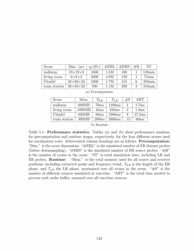
Scene Dim. (m) ηf (Hz) #ERL #ERS #R ST

walkway 19×19×8 1000 1.5M 100 1 120minliving room 6×8×3 2000 4.9M 129 1 75minCitadel 28×60×32 1000 1.7M 155 6 350mintrain station 36×83×32 500 1.1M 200 3 310min

(a) Precomputation

Scene Mem. TER TLR #S ABT

walkway 600MB 70ms 1100ms 1 1.7msliving room 1000MB 45ms 250ms 2 1.8msCitadel 620MB 80ms 1900ms 8 27.2mstrain station 390MB 200ms 2600ms �15 60ms

(b) Runtime

Table 5.1: Performance statistics. Tables (a) and (b) show performance numbersfor precomputation and runtime stages, respectively, for the four different scenes usedfor auralization tests. Abbreviated column headings are as follows. Precomputation:“Dim.” is the scene dimensions. “#ERL” is the simulated number of ER listener probes(before downsampling). “#ERS” is the simulated number of ER source probes. “#R”is the number of rooms in the scene. “ST” is total simulation time, including LR andER probes. Runtime: “Mem.” is the total memory used for all source and receiverpositions, including extracted peaks and frequency trend. TER is the length of the ERphase, and TLR the LR phase, maximized over all rooms in the scene. “#S” is thenumber of different sources simulated at run-time. “ABT” is the total time needed toprocess each audio buffer, summed over all run-time sources.

142

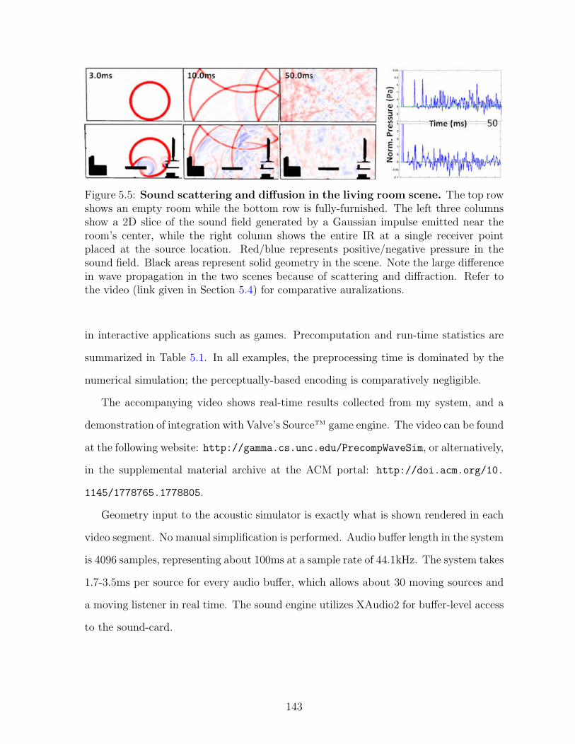
Figure 5.5: Sound scattering and diffusion in the living room scene. The top rowshows an empty room while the bottom row is fully-furnished. The left three columnsshow a 2D slice of the sound field generated by a Gaussian impulse emitted near theroom’s center, while the right column shows the entire IR at a single receiver pointplaced at the source location. Red/blue represents positive/negative pressure in thesound field. Black areas represent solid geometry in the scene. Note the large differencein wave propagation in the two scenes because of scattering and diffraction. Refer tothe video (link given in Section 5.4) for comparative auralizations.

in interactive applications such as games. Precomputation and run-time statistics are

summarized in Table 5.1. In all examples, the preprocessing time is dominated by the

numerical simulation; the perceptually-based encoding is comparatively negligible.

The accompanying video shows real-time results collected from my system, and a

demonstration of integration with Valve’s SourceTM game engine. The video can be found

at the following website: http://gamma.cs.unc.edu/PrecompWaveSim, or alternatively,

in the supplemental material archive at the ACM portal: http://doi.acm.org/10.

1145/1778765.1778805.

Geometry input to the acoustic simulator is exactly what is shown rendered in each

video segment. No manual simplification is performed. Audio buffer length in the system

is 4096 samples, representing about 100ms at a sample rate of 44.1kHz. The system takes

1.7-3.5ms per source for every audio buffer, which allows about 30 moving sources and

a moving listener in real time. The sound engine utilizes XAudio2 for buffer-level access

to the sound-card.

143

5.4.1 Living room

My technique handles complex scenes like the furnished living room shown in Figure 5.4a.

Scattering off furnishings has a noticeable effect on a room’s acoustics. Figure 5.5 com-

pares visualizations of the sound field in a 2D slice of this scene, between the furnished

room and an empty version with all interior objects and carpet removed. In the empty

room, specular wavefronts dominate the sound field and substantial energy still remains

after 50ms. In the furnished room, the greater scattering and larger absorbing surface

area more quickly reduce the sound field’s coherence and energy. Refer to the accom-

panying video to hear the difference. The right column of the figure plots pressure as

a function of time at a single receiver location. The empty room’s IR is dominated by

high, positive-amplitude peaks, while the furnished room’s contains negative pressure

peaks due to diffraction at geometric discontinuities and more closely resembles a real

room’s response qualitatively.

5.4.2 Walkway

Figure 5.4b shows an outdoor scene designed to demonstrate various acoustic effects.

Scene surfaces are all highly reflective with a pressure reflection coefficient of 0.95. Spec-

ular reflections from the walls and lack of scattering yield a fairly long TLR=1.1s, with

a characteristic hollow reverberation due to the parallel walls and lack of intervening

geometry. The walkway’s concave ceiling (blue) focuses sounds, so that they become

louder when the source and receiver both move below it. Occlusion effects are also im-

portant in this scene because diffraction is the only major source of energy transport

behind the walls. The sound loudness changes realistically and smoothly as the listener

walks behind a wall separating him from the source, and demonstrates a convincing

diffracted shadowing effect. Refer to the video for the auralization.

144

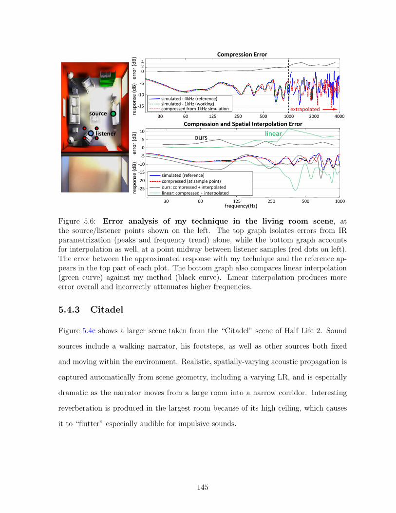
30 60 125 250 500 1000 2000 4000

Compression Error

resp

onse

(dB)

er

ror (

dB)

simulated - 4kHz (reference) simulated - 1kHz (working) compressed from 1kHz simulation

source

listener

30 60 125 250 500 1000

-15

-10

-5

0 2 4

-25

-20

-15

-10

-5

0

5

10 Compression and Spatial Interpolation Error

frequency(Hz)

resp

onse

(dB)

erro

r (dB

)

simulated (reference) compressed (at sample point) ours: compressed + interpolated linear: compressed + interpolated

extrapolated

ours linear

Figure 5.6: Error analysis of my technique in the living room scene, atthe source/listener points shown on the left. The top graph isolates errors from IRparametrization (peaks and frequency trend) alone, while the bottom graph accountsfor interpolation as well, at a point midway between listener samples (red dots on left).The error between the approximated response with my technique and the reference ap-pears in the top part of each plot. The bottom graph also compares linear interpolation(green curve) against my method (black curve). Linear interpolation produces moreerror overall and incorrectly attenuates higher frequencies.

5.4.3 Citadel

Figure 5.4c shows a larger scene taken from the “Citadel” scene of Half Life 2. Sound

sources include a walking narrator, his footsteps, as well as other sources both fixed

and moving within the environment. Realistic, spatially-varying acoustic propagation is

captured automatically from scene geometry, including a varying LR, and is especially

dramatic as the narrator moves from a large room into a narrow corridor. Interesting

reverberation is produced in the largest room because of its high ceiling, which causes

it to “flutter” especially audible for impulsive sounds.

145

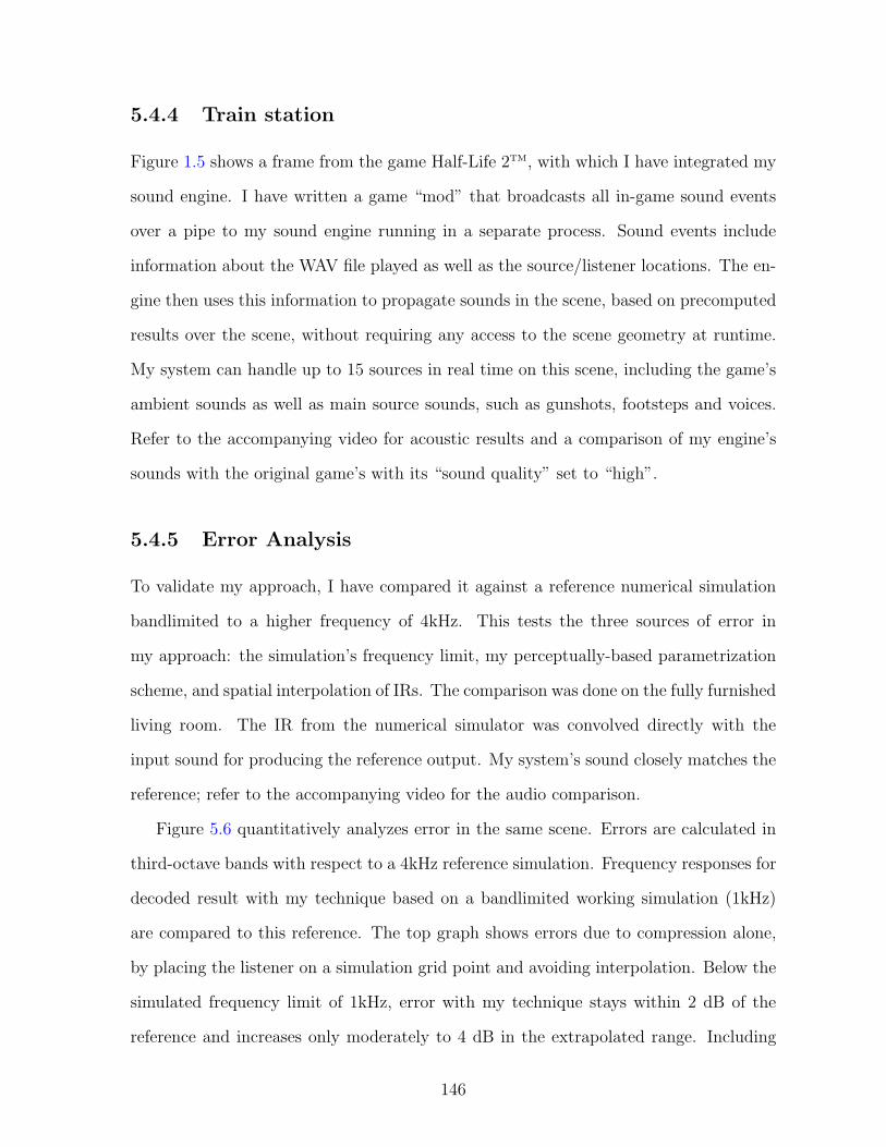
5.4.4 Train station

Figure 1.5 shows a frame from the game Half-Life 2TM, with which I have integrated my

sound engine. I have written a game “mod” that broadcasts all in-game sound events

over a pipe to my sound engine running in a separate process. Sound events include

information about the WAV file played as well as the source/listener locations. The en-

gine then uses this information to propagate sounds in the scene, based on precomputed

results over the scene, without requiring any access to the scene geometry at runtime.

My system can handle up to 15 sources in real time on this scene, including the game’s

ambient sounds as well as main source sounds, such as gunshots, footsteps and voices.

Refer to the accompanying video for acoustic results and a comparison of my engine’s

sounds with the original game’s with its “sound quality” set to “high”.

5.4.5 Error Analysis

To validate my approach, I have compared it against a reference numerical simulation

bandlimited to a higher frequency of 4kHz. This tests the three sources of error in

my approach: the simulation’s frequency limit, my perceptually-based parametrization

scheme, and spatial interpolation of IRs. The comparison was done on the fully furnished

living room. The IR from the numerical simulator was convolved directly with the

input sound for producing the reference output. My system’s sound closely matches the

reference; refer to the accompanying video for the audio comparison.

Figure 5.6 quantitatively analyzes error in the same scene. Errors are calculated in

third-octave bands with respect to a 4kHz reference simulation. Frequency responses for

decoded result with my technique based on a bandlimited working simulation (1kHz)

are compared to this reference. The top graph shows errors due to compression alone,

by placing the listener on a simulation grid point and avoiding interpolation. Below the

simulated frequency limit of 1kHz, error with my technique stays within 2 dB of the

reference and increases only moderately to 4 dB in the extrapolated range. Including

146

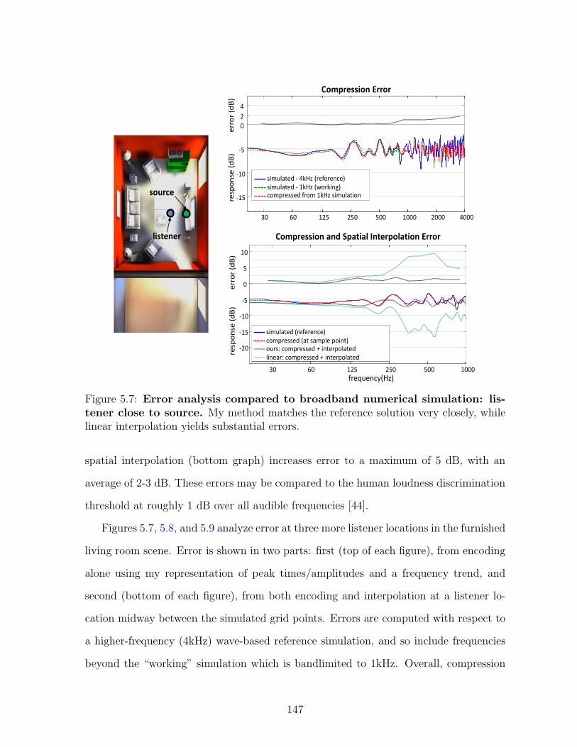
30 60 125 250 500 1000 2000 4000

-15

-10

-5

0 2 4

Compression Error

resp

onse

(dB)

e

rror

(dB)

simulated - 4kHz (reference) simulated - 1kHz (working) compressed from 1kHz simulation

30 60 125 250 500 1000

-20

-15

-10

-5

0

5

10

Compression and Spatial Interpolation Error

frequency(Hz)

resp

onse

(dB)

er

ror (

dB)

simulated (reference) compressed (at sample point) ours: compressed + interpolated linear: compressed + interpolated

source

listener

Figure 5.7: Error analysis compared to broadband numerical simulation: lis-tener close to source. My method matches the reference solution very closely, whilelinear interpolation yields substantial errors.

spatial interpolation (bottom graph) increases error to a maximum of 5 dB, with an

average of 2-3 dB. These errors may be compared to the human loudness discrimination

threshold at roughly 1 dB over all audible frequencies [44].

Figures 5.7, 5.8, and 5.9 analyze error at three more listener locations in the furnished

living room scene. Error is shown in two parts: first (top of each figure), from encoding

alone using my representation of peak times/amplitudes and a frequency trend, and

second (bottom of each figure), from both encoding and interpolation at a listener lo-

cation midway between the simulated grid points. Errors are computed with respect to

a higher-frequency (4kHz) wave-based reference simulation, and so include frequencies

beyond the “working” simulation which is bandlimited to 1kHz. Overall, compression

147

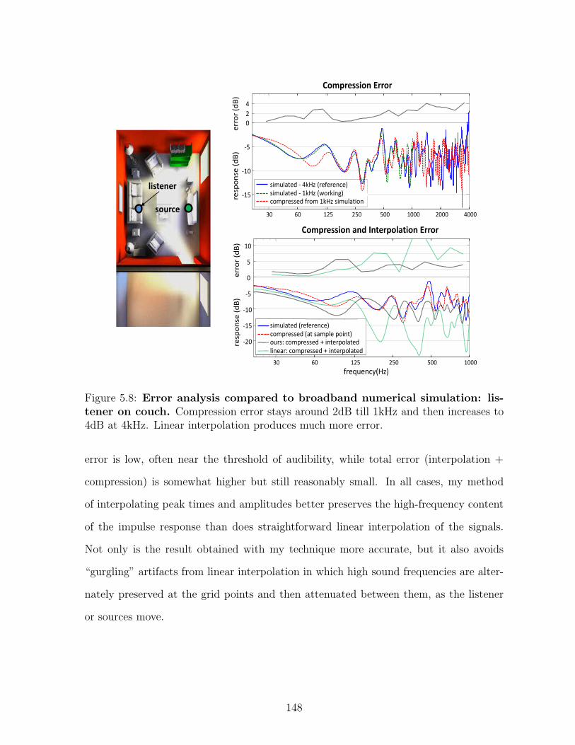
30 60 125 250 500 1000 2000 4000

-15

-10

-5

0 2 4

Compression Error

resp

onse

(dB)

e

rror

(dB)

simulated - 4kHz (reference) simulated - 1kHz (working) compressed from 1kHz simulation

30 60 125 250 500 1000

-20

-15

-10

-5

0

5

10

Compression and Interpolation Error

frequency(Hz)

resp

onse

(dB)

e

rror

(dB)

simulated (reference) compressed (at sample point) ours: compressed + interpolated linear: compressed + interpolated

source

listener

Figure 5.8: Error analysis compared to broadband numerical simulation: lis-tener on couch. Compression error stays around 2dB till 1kHz and then increases to4dB at 4kHz. Linear interpolation produces much more error.

error is low, often near the threshold of audibility, while total error (interpolation +

compression) is somewhat higher but still reasonably small. In all cases, my method

of interpolating peak times and amplitudes better preserves the high-frequency content

of the impulse response than does straightforward linear interpolation of the signals.

Not only is the result obtained with my technique more accurate, but it also avoids

“gurgling” artifacts from linear interpolation in which high sound frequencies are alter-

nately preserved at the grid points and then attenuated between them, as the listener

or sources move.

148

source

listener

30 60 125 250 500 1000 -40 -35 -30 -25 -20 -15 -10 -5 0 5

10

Compression and Spatial Interpolation Errors

frequency(Hz)

resp

onse

(dB)

erro

r (dB

)

simulated (reference) compressed (at sample point) ours: compressed + interpolated linear: compressed + interpolated

30 60 125 250 500 1000 2000 4000

-30

-25

-20

-15

-10

-5

0 2 4

Compression Error

res

pons

e (d

B)

err

or (d

B)

simulated - 4kHz (reference) simulated - 1kHz (working) compressed from 1kHz simulation

Figure 5.9: Error analysis compared to broadband numerical simulation: lis-tener outside door. Sound from the source undergoes multiple scattering in the room,then diffracts around the door to arrive at the listener. Such high-order effects are veryhard to model convincingly and a challenging case for current systems. Notice the clearlow-pass filtering in the frequency response plotted and audible in the demo. Compres-sion error lies between 2 to 4 dB, which is quite low. Spatial interpolation errors arehigher, crossing 5 dB, but my technique produces less error over all frequencies thanlinear interpolation.

149

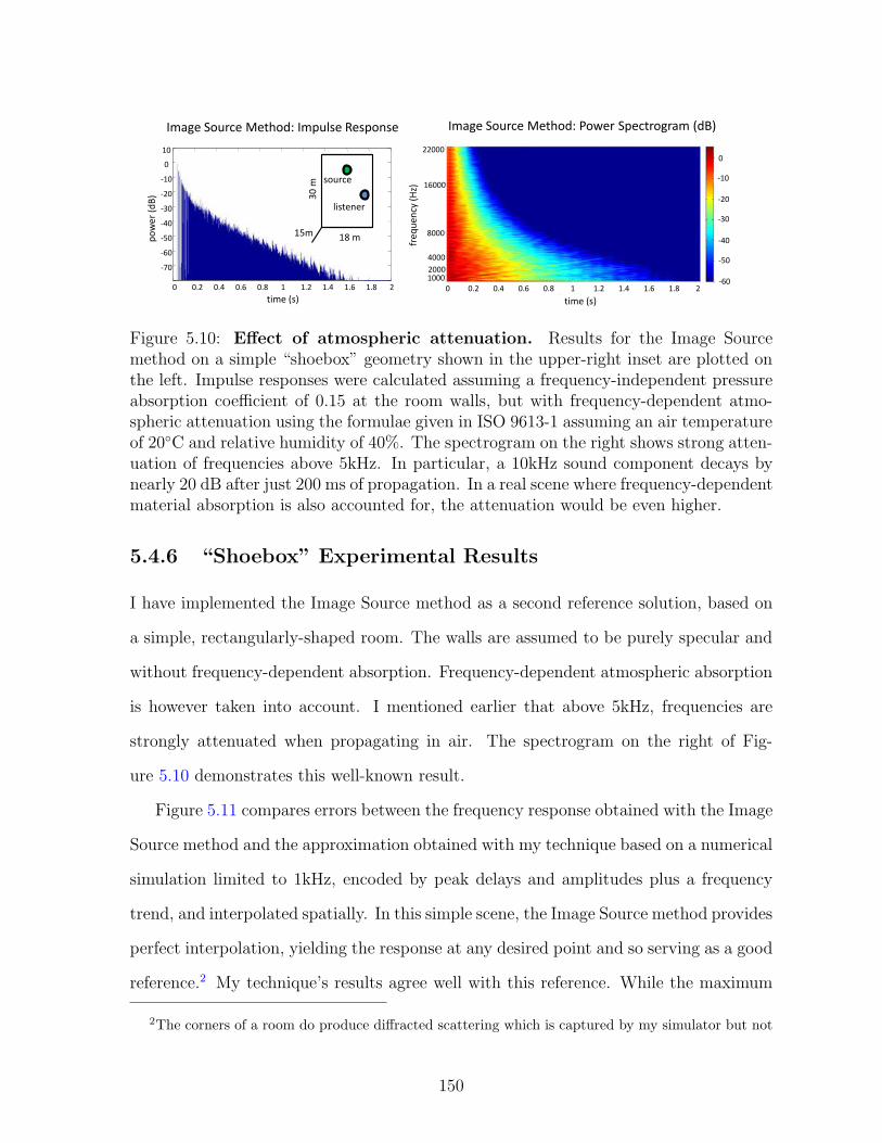
0 0.2 0.4 0.6 0.8 1 1.2 1.4 1.6 1.8 2

-70

-60

-50

-40

-30

-20

-10

0

10

Image Source Method: Impulse Response

time (s)

pow

er (d

B)

freq

uenc

y (H

z)

1000 2000 4000

8000

16000

22000

time (s) 0 0.2 0.4 0.6 0.8 1 1.2 1.4 1.6 1.8 2

0

-10

-20

-30

-40

-50

-60

Image Source Method: Power Spectrogram (dB)

18 m

30 m

source

listener

15m

Figure 5.10: Effect of atmospheric attenuation. Results for the Image Sourcemethod on a simple “shoebox” geometry shown in the upper-right inset are plotted onthe left. Impulse responses were calculated assuming a frequency-independent pressureabsorption coefficient of 0.15 at the room walls, but with frequency-dependent atmo-spheric attenuation using the formulae given in ISO 9613-1 assuming an air temperatureof 20◦C and relative humidity of 40%. The spectrogram on the right shows strong atten-uation of frequencies above 5kHz. In particular, a 10kHz sound component decays bynearly 20 dB after just 200 ms of propagation. In a real scene where frequency-dependentmaterial absorption is also accounted for, the attenuation would be even higher.

5.4.6 “Shoebox” Experimental Results

I have implemented the Image Source method as a second reference solution, based on

a simple, rectangularly-shaped room. The walls are assumed to be purely specular and

without frequency-dependent absorption. Frequency-dependent atmospheric absorption

is however taken into account. I mentioned earlier that above 5kHz, frequencies are

strongly attenuated when propagating in air. The spectrogram on the right of Fig-

ure 5.10 demonstrates this well-known result.

Figure 5.11 compares errors between the frequency response obtained with the Image

Source method and the approximation obtained with my technique based on a numerical

simulation limited to 1kHz, encoded by peak delays and amplitudes plus a frequency

trend, and interpolated spatially. In this simple scene, the Image Source method provides

perfect interpolation, yielding the response at any desired point and so serving as a good

reference.2 My technique’s results agree well with this reference. While the maximum

2The corners of a room do produce diffracted scattering which is captured by my simulator but not

150

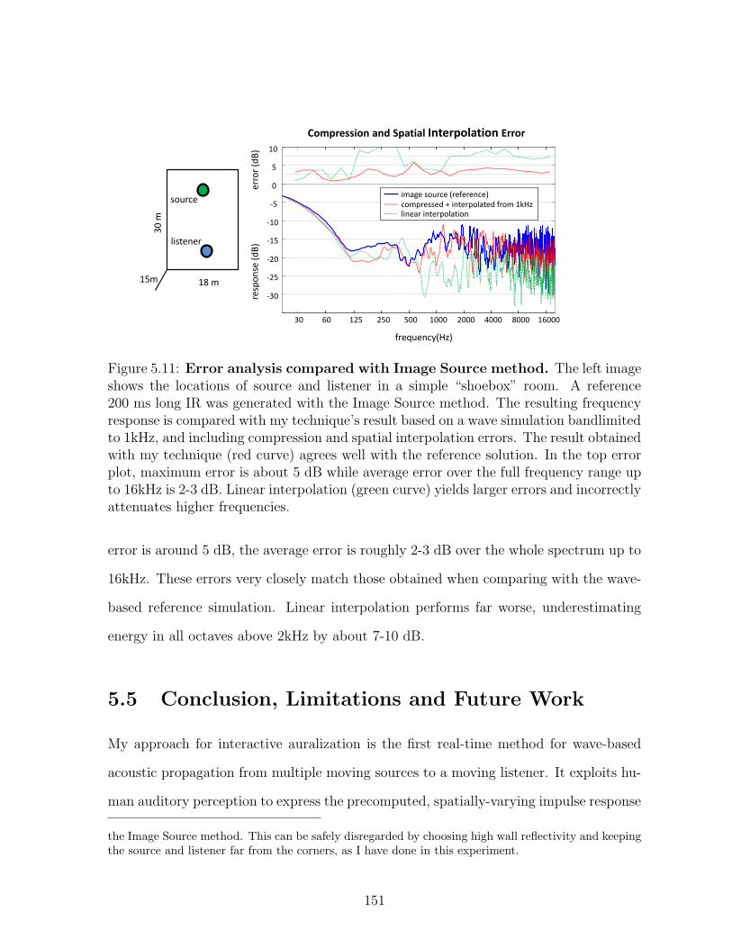
30 60 125 250 500 1000 2000 4000 8000 16000

-30

-25

-20

-15

-10

-5

0

5

10

Compression and Spatial Interpolation Error

frequency(Hz)

resp

onse

(dB)

erro

r (dB

)

image source (reference) compressed + interpolated from 1kHz linear interpolation

30 m

source

listener

15m 18 m

Figure 5.11: Error analysis compared with Image Source method. The left imageshows the locations of source and listener in a simple “shoebox” room. A reference200 ms long IR was generated with the Image Source method. The resulting frequencyresponse is compared with my technique’s result based on a wave simulation bandlimitedto 1kHz, and including compression and spatial interpolation errors. The result obtainedwith my technique (red curve) agrees well with the reference solution. In the top errorplot, maximum error is about 5 dB while average error over the full frequency range upto 16kHz is 2-3 dB. Linear interpolation (green curve) yields larger errors and incorrectlyattenuates higher frequencies.

error is around 5 dB, the average error is roughly 2-3 dB over the whole spectrum up to

16kHz. These errors very closely match those obtained when comparing with the wave-

based reference simulation. Linear interpolation performs far worse, underestimating

energy in all octaves above 2kHz by about 7-10 dB.

5.5 Conclusion, Limitations and Future Work

My approach for interactive auralization is the first real-time method for wave-based

acoustic propagation from multiple moving sources to a moving listener. It exploits hu-

man auditory perception to express the precomputed, spatially-varying impulse response

the Image Source method. This can be safely disregarded by choosing high wall reflectivity and keepingthe source and listener far from the corners, as I have done in this experiment.

151

of a complex but static scene in a compact form. My run-time technique convolves in

the frequency-domain, allowing arbitrarily dense impulse responses. Overall, my sys-

tem captures realistic acoustic effects including late reverberation, diffuse reflections,

reverberation coloration, sound focusing, and diffraction low-pass filtering around ob-

structions.

Some limitations of my approach are due to the high computational cost of wave

simulators on today’s desktops – the simulation’s frequency limit and restricted volume.

Others arise from precomputation – the restriction to static scenes and high runtime

memory use (hundreds of MBs) even with fairly low spatial sampling. Memory use

could be reduced by extracting an even more compact set of ERIR perceptual param-

eters such as loudness, clarity, etc. Finding a “perceptually complete” set is an open

research problem, as is determining spatial sampling requirements for perceptually ac-

curate auralization. My technique might be practically extended to dynamic scenes

by simulating low-dimensional parameterized scenes, such as an opera house at vari-

ous degrees of seating occupation. It could also benefit from approximations to handle

dynamic objects, perhaps by separately precomputing frequency-dependent occlusion

factors and then applying them on the fly.

152

Chapter 6

Conclusion and Future Work

The contributions of my dissertation lie in the three inter-connected sub-problems of

Physically-based Sound Simulation – Interactive Sound Synthesis, Numerical Acoustics

Simulation and Interactive Sound Propagation. In the area of Interactive Sound Syn-

thesis, I have presented techniques that exploit human auditory perception, such as its

limited frequency resolution, to deliver large gains in performance. The system I have

developed has been integrated with existing physics engines such as ODE and NVIDIA

PhysX, to enable interactive applications with hundreds of sounding objects undergo-

ing impacts and rolling, resulting in richly interactive applications with realistic sound.

The second part of my work is on performing fast numerical acoustic simulations that

are hundred times faster than a high-oder finite difference technique. This is achieved

by exploiting known analytical solutions for the Wave Equation and decomposing the

simulation domain into rectangular partitions. This enables acoustic prediction on large

scenes that were intractable earlier on a desktop computer – simulations that would

have taken days on a small cluster of processors can be performed in minutes with the

simulator I have developed.

Lastly, I have developed the first interactive auralization system to utilize wave-

based acoustics for arbitrary static scenes with complex geometry and be able to handle

moving sound sources and listener. My system is capable of automatically handling

commonly perceivable acoustic effects such sound focusing, low-pass filtering due to

occlusion/obstruction, realistic reverberation, and diffuse reflections. Prior techniques

relying on geometric methods have difficulty handling diffraction and high-order reflec-

tions. The key idea behind this technique is a compact representation that captures

the perceptually salient aspects of acoustics responses. This representation allows a

reduction of memory usage by a factor of up to thousand times compared to a simple,

direct storage scheme. In addition to this, I have developed an auralization system that

performs perceptually realistic interpolation of impulse responses stored in this com-

pact representation, and performs fast convolutions in frequency domain to render the

acoustics in real time.

The Future: Over the past few decades, the area of computer graphics has seen a

synergistic development of computational techniques, perceptual approximations, and

computational power, that has enabled the stunning visual realism of interactive appli-

cations today. Based on my experience working on this thesis and the increasing amount

of concurrent work in this area, I believe that interactive sound simulation is following

the same trend. The development of graphics processors has largely removed the burden

of graphics computations from the CPU. In addition, graphics processors offer massive

parallelism, that can be helpful for accelerating precomputation for sound simulation, as

I have shown for the ARD technique. Furthermore, there is an increasing trend towards

multi-core processors – the Xbox 360 gaming console released in 2005 already had three

cores and high-end, quad-core desktop system are easily available today. Therefore, the

amount of computation available for audio is increasing consistently over time. What

is needed is continued development of fast algorithms and approximations based on our

current (and improving) understanding of psycho-acoustics to design ever more efficient

algorithms to translate this available computational power into a compelling overall

aural experience, at interactive speeds.

154

There are many interesting areas for future research in interactive sound simulation.

Perhaps the most general theme to be explored is a systematic study of the limits of

auditory perception in the context of interactive applications and human error toler-

ances while approximating different aural phenomena, whether in the context of sound

synthesis, or propagation. Existing wisdom from other areas of research, such as room

acoustics, speech synthesis and musical synthesis would surely inform such work, as is

the case for this thesis. However, I am quite certain that new studies specific to inter-

active applications will be required, since some questions arise that are very specific to

this area. As an example, it would be very useful to study the tolerable errors in sound

propagation for moving sources and listener, as this would give valuable insights into

approximations that work for acoustic responses in such cases.

The first and foremost requirement for such systematic studies seems to be finding a

“perceptually complete” set of parameters and their associated error tolerance values for

humans. In addition to traditionally used quantities, such as loudness, I am sure such a

list would also contain far more detailed quantities relating to the spectral content and its

time-varying nature. This would prove invaluable for research in this area, serving as an

essential guideline for designing perceptually realistic interactive techniques for sound

simulation, and informing any such technique about the ultimate limits of efficiency

gains from perceptually-based approximations. I am sure that this would be a very

rewarding direction, and might even contribute to research in psychoacoustics as well –

interactive virtual environments can potentially be a very useful tool for psychoacoustic

studies.

There are many future directions possible in the area of sound synthesis. Interactive

sound synthesis is a very nascent area, and there is a large variety of sounds that have

seen limited exploration (or none at all), that can possibly yield to interactive synthesis

through an understanding of their underlying physics, as well as perception. To give a

non-exhaustive list here – cloth sounds, efficient sliding and rolling sounds, explosions,

155

creaking, liquids, footsteps, fracture and engine sounds. Simulating all of these sounds

would add a new layer of immersion to existing interactive applications.

In the area of acoustics, my work has shown that significant compression can be

achieved for storing the results of wave simulation. However, I am sure that a lot

more compression can still be achieved. The first step would be to find a perceptually

sufficient set of perceptually important acoustic parameters. The acoustic responses

would then be stored as lists of these parameters alone. Such development, coupled

with the development of scalable, fast, and memory-efficient acoustic techniques that can

handle indoor and outdoor scenes with equal ease, would allow interactive applications

to make a large step in terms of the realism achieved. However, the challenge of designing

such techniques is quite similar to what global illumination research in graphics has faced

over the years. I am sure that this challenge can be met by a combination of increasing

computational power and improved numerical techniques that rely on physics as well as

perception.

The impact of such sound synthesis and propagation techniques would extend beyond

just game or movie studios – we are seeing the rise of massively multi-player immersive

worlds that let the players collaboratively build environments and objects of their own.

What if you make a “virtual” wooden bowl and it automatically sounds like one? What

if you build a house and its acoustics automatically corresponds to what would be

expected in reality? How does it sound if you drop the bowl in your house’s kitchen?

Obviously, this problem is quite impractical with pre-recorded sounds and filters mainly

because the scene doesn’t exist in reality and thus recording the information might not

even be possible. Moreover, the process of applying such prerecorded information is very

unintuitive – in real life you don’t make an object and then cast a magic spell to assign

some sound to it. The same should apply for the virtual world – by virtue of designing

an object, it should have visual as well as aural properties automatically. What I have

described can be potentially achieved in the future, and my work has served as a step in

156

this direction. But as I have conveyed, a large number of very interesting and challenging

research problems still need to be solved. There are many possible improvements to the

techniques I have described in this thesis, which I have discussed individually. The hope

is that in the future we will be seeing more and more virtual worlds which will integrate

realistic physically-based sounds, and combined with ever-improving graphics, give us a

visceral feeling – “I am here”.

157

Bibliography

[1] Domain decomposition method. http://www.ddm.org. 60

[2] The havok physics engine. http://www.havok.com/. 25

[3] The nvidia physx physics engine. http://www.nvidia.com/object/physx new.html.

25

[4] The open dynamics engine. http://www.ode.org/. 25

[5] Soundscapes in half-life 2, valve corporation.

http://developer.valvesoftware.com/wiki/Soundscapes, 2008. 30

[6] J. B. Allen and D. A. Berkley. Image method for efficiently simulating small-room

acoustics. J. Acoust. Soc. Am, 65(4):943–950, 1979. 52

[7] F. Antonacci, M. Foco, A. Sarti, and S. Tubaro. Real time modeling of acoustic

propagation in complex environments. Proceedings of 7th International Conference

on Digital Audio Effects, pages 274–279, 2004. 52

[8] M. Bertram, E. Deines, J. Mohring, J. Jegorovs, and H. Hagen. Phonon tracing

for auralization and visualization of sound. In IEEE Visualization 2005, pages

151–158, 2005. 52

[9] Stefan Bilbao. Wave and Scattering Methods for Numerical Simulation. Wiley,

July 2004. 58

[10] J. Blauert. An introduction to binaural technology. In R. Gilkey and T. R. An-

derson, editors, Binaural and Spatial Hearing in Real and Virtual Environments.

Lawrence Erlbaum, USA, 1997. 11, 139

[11] Nicolas Bonneel, George Drettakis, Nicolas Tsingos, Isabelle V. Delmon, and Doug

James. Fast modal sounds with scalable frequency-domain synthesis. ACM Trans-

actions on Graphics (SIGGRAPH Conference Proceedings), 27(3), 2008. 47

[12] D. Botteldooren. Acoustical finite-difference time-domain simulation in a quasi-

cartesian grid. The Journal of the Acoustical Society of America, 95(5):2313–2319,

1994. 58

158

[13] D. Botteldooren. Finite-difference time-domain simulation of low-frequency room

acoustic problems. Acoustical Society of America Journal, 98:3302–3308, Decem-

ber 1995. 58

[14] John P. Boyd. Chebyshev and Fourier Spectral Methods: Second Revised Edition.

Dover Publications, 2 revised edition, December 2001. 60

[15] Paul Calamia. Advances in Edge-Diffraction Modeling for Virtual-Acoustic Simu-

lations. PhD thesis, Princeton University, June 2009. 36, 52, 53, 62

[16] Jeffrey N. Chadwick, Steven S. An, and Doug L. James. Harmonic shells: a

practical nonlinear sound model for near-rigid thin shells. In SIGGRAPH Asia

’09: ACM SIGGRAPH Asia 2009 papers, pages 1–10, New York, NY, USA, 2009.

ACM. 48

[17] A. Chaigne and V. Doutaut. Numerical simulations of xylophones. i. time domain

modeling of the vibrating bars. J. Acoust. Soc. Am., 101(1):539–557, 1997. 26,

45, 86

[18] Anish Chandak, Christian Lauterbach, Micah Taylor, Zhimin Ren, and Dinesh

Manocha. Ad-frustum: Adaptive frustum tracing for interactive sound propaga-

tion. IEEE Transactions on Visualization and Computer Graphics, 14(6):1707–

1722, 2008. 36, 52, 62

[19] A. Cheng and D. Cheng. Heritage and early history of the boundary element

method. Engineering Analysis with Boundary Elements, 29(3):268–302, March

2005. 56

[20] J. Y. Chung, J.W.S Liu, and K. J. Lin. Scheduling real-time, periodic jobs using

imprecise results. In Proc. IEEE RTS, 1987. 47

[21] Perry R. Cook. Real Sound Synthesis for Interactive Applications (Book & CD-

ROM). AK Peters, Ltd., 1st edition, 2002. 45

[22] Carlos A. de Moura. Parallel numerical methods for differential equations - a

survey. 59, 100

[23] Yoshinori Dobashi, Tsuyoshi Yamamoto, and Tomoyuki Nishita. Real-time ren-

dering of aerodynamic sound using sound textures based on computational fluid

159

dynamics. ACM Trans. Graph., 22(3):732–740, July 2003. 48

[24] Yoshinori Dobashi, Tsuyoshi Yamamoto, and Tomoyuki Nishita. Synthesizing

sound from turbulent field using sound textures for interactive fluid simulation.

Computer Graphics Forum (Proc. EUROGRAPHICS 2004), 23(3):539–546, 2004.

48

[25] Jack Dongarra. Performance of various computers using standard linear equa-

tions software. Technical report, Electrical Engineering and Computer Science

Department, University of Tennessee, Knoxville, TN 37996-1301, 2008. 73

[26] Durlach. Virtual reality scientific and technological challenges. Technical report,

National Research Council, 1995. 14

[27] M. David Egan. Architectural Acoustics (J. Ross Publishing Classics). J. Ross

Publishing, January 2007. 4, 49

[28] M. Emerit, J. Faure, A. Guerin, R. Nicol, G. Pallone, P. Philippe, and D. Virette.

Efficient binaural filtering in QMF domain for BRIR. In AES 122th Convention,

May 2007. 65

[29] Thomas Ertl, Ken Joy, Beatriz S. Editors, E. Deines, F. Michel, M. Bertram,

H. Hagen, and G. M. Nielson. Visualizing the phonon map. In IEEE-VGTC

Symposium on Visualization, 2006. 52

[30] J. L. Florens and C. Cadoz. The physical model: modeling and simulating the

instrumental universe. In G. D. Poli, A. Piccialli, and C. Roads, editors, Repre-

senations of Musical Signals, pages 227–268. MIT Press, Cambridge, MA, USA,

1991. 45

[31] H. Fouad, J. Ballas, and J. Hahn. Perceptually based scheduling algorithms for

real-time synthesis of complex sonic environments. In Proc. Int. Conf. Auditory

Display, 1997. 47

[32] M. Frigo and S. G. Johnson. The design and implementation of fftw3. Proc. IEEE,

93(2):216–231, 2005. 95, 114

[33] Thomas Funkhouser, Nicolas Tsingos, Ingrid Carlbom, Gary Elko, Mohan Sondhi,

James E. West, Gopal Pingali, Patrick Min, and Addy Ngan. A beam tracing

160

method for interactive architectural acoustics. The Journal of the Acoustical So-

ciety of America, 115(2):739–756, 2004. 36, 52, 62

[34] W. G. Gardner. Reverberation algorithms. In M. Kahrs and K. Brandenburg,

editors, Applications of Digital Signal Processing to Audio and Acoustics (The

Springer International Series in Engineering and Computer Science), pages 85–

131. Springer, 1 edition, 1998. 64, 125, 129

[35] Carolyn Gordon, David L. Webb, and Scott Wolpert. One cannot hear the shape

of a drum. Bulletin of the American Mathematical Society (N.S.), 27(1):134–138,

1992. 11

[36] Naga K. Govindaraju, Brandon Lloyd, Yuri Dotsenko, Burton Smith, and John

Manferdelli. High performance discrete fourier transforms on graphics processors.

In SC ’08: Proceedings of the 2008 ACM/IEEE conference on Supercomputing,

pages 1–12, Piscataway, NJ, USA, 2008. IEEE Press. 32, 113

[37] Eran Guendelman, Robert Bridson, and Ronald Fedkiw. Nonconvex rigid bodies

with stacking. ACM Trans. Graph., 22(3):871–878, July 2003. 81

[38] Nail A. Gumerov and Ramani Duraiswami. Fast multipole methods on graphics

processors. J. Comput. Phys., 227(18):8290–8313, September 2008. 56, 57

[39] Nail A. Gumerov and Ramani Duraiswami. A broadband fast multipole acceler-

ated boundary element method for the three dimensional helmholtz equation. The

Journal of the Acoustical Society of America, 125(1):191–205, 2009. 56

[40] Tor Halmrast. Coloration due to reflections. further investigations. In Interna-

tional Congress on Acoustics, September 2007. 124

[41] W. M. Hartmann and A. Wittenberg. On the externalization of sound images.

The Journal of the Acoustical Society of America, 99(6):3678–3688, June 1996.

139

[42] Murray Hodgson and Eva M. Nosal. Experimental evaluation of radiosity for

room sound-field prediction. The Journal of the Acoustical Society of America,

120(2):808–819, 2006. 52

[43] Doug L. James, Jernej Barbic, and Dinesh K. Pai. Precomputed acoustic transfer:

161

output-sensitive, accurate sound generation for geometrically complex vibration

sources. ACM Transactions on Graphics, 25(3):987–995, July 2006. 63

[44] Walt Jesteadt, Craig C. Wier, and David M. Green. Intensity discrimination as

a function of frequency and sensation level. The Journal of the Acoustical Society

of America, 61(1):169–177, 1977. 147

[45] Matti Karjalainen and Cumhur Erkut. Digital waveguides versus finite difference

structures: equivalence and mixed modeling. EURASIP J. Appl. Signal Process.,

2004(1):978–989, January 2004. 55, 57, 58

[46] Young J. Kim, Ming C. Lin, and Dinesh Manocha. Deep: Dual-space expansion for

estimating penetration depth between convex polytopes. In IEEE International

Conference on Robotics and Automation, May 2002. 81

[47] Lawrence E. Kinsler, Austin R. Frey, Alan B. Coppens, and James V. Sanders.

Fundamentals of acoustics. Wiley, 4 edition, December 2000. 29, 49

[48] Mendel Kleiner, Bengt-Inge Dalenback, and Peter Svensson. Auralization - an

overview. JAES, 41:861–875, 1993. 55

[49] K. Kowalczyk and M. van Walstijn. Room acoustics simulation using 3-d com-

pact explicit fdtd schemes. IEEE Transactions on Audio, Speech and Language

Processing, 2010. 58, 103, 119

[50] A. Krokstad, S. Strom, and S. Sorsdal. Calculating the acoustical room response

by the use of a ray tracing technique. Journal of Sound and Vibration, 8(1):118–

125, July 1968. 52

[51] Heinri Kuttruff. Room Acoustics. Taylor & Francis, October 2000. 31, 35, 37, 49,

94, 112, 122, 124, 127, 129, 134

[52] Tobias Lentz, Dirk Schroder, Michael Vorlander, and Ingo Assenmacher. Virtual

reality system with integrated sound field simulation and reproduction. EURASIP

J. Appl. Signal Process., 2007(1):187, 2007. 61

[53] Ruth Y. Litovsky, Steven H. Colburn, William A. Yost, and Sandra J. Guz-

man. The precedence effect. The Journal of the Acoustical Society of America,

106(4):1633–1654, 1999. 123

162

[54] Qing H. Liu. The pstd algorithm: A time-domain method combining the pseu-

dospectral technique and perfectly matched layers. The Journal of the Acoustical

Society of America, 101(5):3182, 1997. 60, 93

[55] T. Lokki. Physically-based Auralization. PhD thesis, Helsinki University of Tech-

nology, 2002. 61

[56] C. Masterson, G. Kearney, and F. Boland. Acoustic impulse response interpolation

for multichannel systems using dynamic time warping. In 35th AES Conference

on Audio for Games, 2009. 65

[57] Ravish Mehra, Nikunj Raghuvanshi, Ming Lin, and Dinesh Manocha. Efficient

gpu-based solver for acoustic wave equation. Technical report, Department of

Computer Science, UNC Chapel Hill, USA, 2010. 101, 120

[58] P. Min and T. Funkhouser. Priority-driven acoustic modeling for virtual environ-

ments. Computer Graphics Forum, pages 179–188, September 2000. 64

[59] Brian Mirtich and John Canny. Impulse-based simulation of rigid bodies. In I3D

’95: Proceedings of the 1995 symposium on Interactive 3D graphics, New York,

NY, USA, 1995. ACM. 81

[60] James Moody and Paul Dexter. Concert Lighting, Third Edition: Techniques, Art

and Business. Focal Press, 3 edition, September 2009. 1

[61] William Moss, Hengchin Yeh, Jeong-Mo Hong, Ming C. Lin, and Dinesh Manocha.

Sounding liquids: Automatic sound synthesis from fluid simulation. ACM Trans-

actions on Graphics (proceedings of SIGGRAPH 2010), 29(3), July 2010. 48

[62] D. Murphy, A. Kelloniemi, J. Mullen, and S. Shelley. Acoustic modeling using the

digital waveguide mesh. Signal Processing Magazine, IEEE, 24(2):55–66, 2007.

57, 58

[63] James F. O’Brien, Perry R. Cook, and Georg Essl. Synthesizing sounds from

physically based motion. In SIGGRAPH ’01: Proceedings of the 28th annual

conference on Computer graphics and interactive techniques, pages 529–536, New

York, NY, USA, 2001. ACM Press. 26, 45

[64] James F. O’Brien, Chen Shen, and Christine M. Gatchalian. Synthesizing sounds

163

from rigid-body simulations. In The ACM SIGGRAPH 2002 Symposium on Com-

puter Animation, pages 175–181. ACM Press, July 2002. 26, 46, 69, 72

[65] R. Petrausch and S. Rabenstein. Simulation of room acoustics via block-based

physical modeling with the functional transformation method. Applications of

Signal Processing to Audio and Acoustics, 2005. IEEE Workshop on, pages 195–

198, 16-19 Oct. 2005. 60

[66] Jackson Pope, David Creasey, and Alan Chalmers. Realtime room acoustics using

ambisonics. In The Proceedings of the AES 16th International Conference on Spa-

tial Sound Reproduction, pages 427–435. Audio Engineering Society, April 1999.

64

[67] Alfio Quarteroni and Alberto Valli. Domain Decomposition Methods for Partial

Differential Equations (Numerical Mathematics and Scientific Computation). Ox-

ford University Press, USA, July 1999. 60

[68] R. Rabenstein, S. Petrausch, A. Sarti, G. De Sanctis, C. Erkut, and M. Kar-

jalainen. Block-based physical modeling for digital sound synthesis. Signal Pro-

cessing Magazine, IEEE, 24(2):42–54, 2007. 60

[69] Nikunj Raghuvanshi, Nico Galoppo, and Ming C. Lin. Accelerated wave-based

acoustics simulation. In SPM ’08: Proceedings of the 2008 ACM symposium on

Solid and physical modeling, pages 91–102, New York, NY, USA, 2008. ACM. 33

[70] Nikunj Raghuvanshi, Christian Lauterbach, Anish Chandak, Dinesh Manocha,

and Ming C. Lin. Real-time sound synthesis and propagation for games. Commun.

ACM, 50(7):66–73, July 2007. 27

[71] Nikunj Raghuvanshi and Ming C. Lin. Interactive sound synthesis for large scale

environments. In SI3D ’06: Proceedings of the 2006 symposium on Interactive 3D

graphics and games, pages 101–108, New York, NY, USA, 2006. ACM Press. 27

[72] Nikunj Raghuvanshi and Ming C. Lin. Physically based sound synthesis for large-

scale virtual environments. IEEE Computer Graphics and Applications, 27(1):14–

18, 2007. 27

[73] Nikunj Raghuvanshi, Brandon Lloyd, Naga K. Govindaraju, and Ming C. Lin.

Efficient numerical acoustic simulation on graphics processors using adaptive rect-

164

angular decomposition. In EAA Symposium on Auralization, June 2009. 33

[74] Nikunj Raghuvanshi, Rahul Narain, and Ming C. Lin. Efficient and accurate

sound propagation using adaptive rectangular decomposition. IEEE Transactions

on Visualization and Computer Graphics, 15(5):789–801, 2009. 33

[75] Nikunj Raghuvanshi, John Snyder, Ravish Mehra, Ming C. Lin, and Naga K.

Govindaraju. Precomputed wave simulation for real-time sound propagation of

dynamic sources in complex scenes. ACM Transactions on Graphics (proceedings

of SIGGRAPH 2010), 29(3), July 2010. 41

[76] Zhimin Ren, Hengchin Yeh, and Ming C. Lin. Synthesizing contact sounds between

textured models. In 2010 IEEE Virtual Reality Conference (VR), pages 139–146.

IEEE, March 2010. 48

[77] Y. S. Rickard, N. K. Georgieva, and Wei-Ping Huang. Application and optimiza-

tion of pml abc for the 3-d wave equation in the time domain. Antennas and

Propagation, IEEE Transactions on, 51(2):286–295, 2003. 103

[78] J. H. Rindel. The use of computer modeling in room acoustics. Journal of Vibro-

engineering, 3(4):219–224, 2000. 52

[79] D. Rizos and S. Zhou. An advanced direct time domain bem for 3-d wave propa-

gation in acoustic media. Journal of Sound and Vibration, 293(1-2):196–212, May

2006. 56

[80] Ton Roosendaal. The blender foundation. http://www.blender.org. 49

[81] H. Sabine. Room acoustics. Audio, Transactions of the IRE Professional Group

on, 1(4):4–12, 1953. 49

[82] S. Sakamoto, T. Yokota, and H. Tachibana. Numerical sound field analysis in

halls using the finite difference time domain method. In RADS 2004, Awaji,

Japan, 2004. 58

[83] Shinichi Sakamoto, Hiroshi Nagatomo, Ayumi Ushiyama, and Hideki Tachibana.

Calculation of impulse responses and acoustic parameters in a hall by the finite-

difference time-domain method. Acoustical Science and Technology, 29(4), 2008.

108

165

[84] Shinichi Sakamoto, Takuma Seimiya, and Hideki Tachibana. Visualization of

sound reflection and diffraction using finite difference time domain method. Acous-

tical Science and Technology, 23(1):34–39, 2002. 58

[85] Shinichi Sakamoto, Ayumi Ushiyama, and Hiroshi Nagatomo. Numerical analysis

of sound propagation in rooms using the finite difference time domain method.

The Journal of the Acoustical Society of America, 120(5):3008, 2006. 58

[86] L. Savioja. Modeling Techniques for Virtual Acoustics. Doctoral thesis, Helsinki

University of Technology, Telecommunications Software and Multimedia Labora-

tory, Report TML-A3, 1999. 51, 57, 61

[87] L. Savioja, J. Backman, A. Jarvinen, and T. Takala. Waveguide mesh method

for low-frequency simulation of room acoustics. In 15th International Congress on

Acoustics (ICA’95), volume 2, pages 637–640, Trondheim, Norway, June 1995. 57

[88] L. Savioja, T. Rinne, and T. Takala. Simulation of room acoustics with a 3-d finite

difference mesh. In Proceedings of the International Computer Music Conference,

pages 463–466, 1994. 58

[89] L. Savioja and V. Valimaki. Interpolated 3-d digital waveguide mesh with fre-

quency warping. In ICASSP ’01: Proceedings of the Acoustics, Speech, and Signal

Processing, 2001. on IEEE International Conference, pages 3345–3348, Washing-

ton, DC, USA, 2001. IEEE Computer Society. 58

[90] Lauri Savioja. Real-time 3d finite-difference time-domain simulation of mid-

frequency room acoustics. In 13th International Conference on Digital Audio

Effects (DAFx-10), September 2010. 58, 59, 103, 119

[91] Lauri Savioja, Jyri Huopaniemi, Tapio Lokki, and Ritta Vaananen. Creating in-

teractive virtual acoustic environments. Journal of the Audio Engineering Society

(JAES), 47(9):675–705, September 1999. 61

[92] A. Sek and B. C. Moore. Frequency discrimination as a function of frequency,

measured in several ways. J. Acoust. Soc. Am., 97(4):2479–2486, April 1995. 47,

73

[93] K. L. Shlager and J. B. Schneider. A selective survey of the finite-difference time-

domain literature. Antennas and Propagation Magazine, IEEE, 37(4):39–57, 1995.

166

58

[94] Samuel Siltanen. Geometry reduction in room acoustics modeling. Master’s thesis,

Helsinki University of Technology, 2005. 36, 51, 106

[95] Julius O. Smith. Physical Audio Signal Processing.

http://ccrma.stanford.edu/˜jos/pasp, 2010. 45

[96] Efstathios Stavrakis, Nicolas Tsingos, and Paul Calamia. Topological sound prop-

agation with reverberation graphs. Acta Acustica/Acustica - the Journal of the

European Acoustics Association (EAA), 2008. 65, 138

[97] C. Stoelinga and A. Chaigne. Time-domain modeling and simulation of rolling

objects. Acustica united with Acta Acustica, 93(2):290–304, 2007. 48

[98] U. Peter Svensson, Paul Calamia, and Shinsuke Nakanishi. Frequency-domain

edge diffraction for finite and infinite edges. In Acta Acustica/Acustica 95, pages

568–572, 2009. 135

[99] Allen Taflove and Susan C. Hagness. Computational Electrodynamics: The Finite-

Difference Time-Domain Method, Third Edition. Artech House Publishers, 3 edi-

tion, June 2005. 44, 58, 60, 92, 108

[100] Tapio Takala and James Hahn. Sound rendering. SIGGRAPH Comput. Graph.,

26(2):211–220, July 1992. 13, 15

[101] Micah T. Taylor, Anish Chandak, Lakulish Antani, and Dinesh Manocha. Re-

sound: interactive sound rendering for dynamic virtual environments. In MM ’09:

Proceedings of the seventeen ACM international conference on Multimedia, pages

271–280, New York, NY, USA, 2009. ACM. 52, 62

[102] Lonny L. Thompson. A review of finite-element methods for time-harmonic acous-

tics. The Journal of the Acoustical Society of America, 119(3):1315–1330, 2006.

55

[103] Rendell R. Torres, U. Peter Svensson, and Mendel Kleiner. Computation of edge

diffraction for more accurate room acoustics auralization. The Journal of the

Acoustical Society of America, 109(2):600–610, 2001. 62

[104] Andrea Toselli and Olof B. Widlund. Domain decomposition methods–algorithms

167

and theory. Springer series in computational mathematics, 34. Springer, 1 edition,

November 2005. 60

[105] Nicolas Tsingos. Simulating High Quality Dynamic Virtual Sound Fields For In-

teractive Graphics Applications. PhD thesis, Universite Joseph Fourier Grenoble

I, December 1998. 52

[106] Nicolas Tsingos. Pre-computing geometry-based reverberation effects for games.

In 35th AES Conference on Audio for Games, 2009. 64, 65

[107] Nicolas Tsingos, Carsten Dachsbacher, Sylvain Lefebvre, and Matteo Dellepiane.

Instant sound scattering. In Rendering Techniques (Proceedings of the Eurograph-

ics Symposium on Rendering), 2007. 63

[108] Nicolas Tsingos, Thomas Funkhouser, Addy Ngan, and Ingrid Carlbom. Model-

ing acoustics in virtual environments using the uniform theory of diffraction. In

SIGGRAPH ’01: Proceedings of the 28th annual conference on Computer graphics

and interactive techniques, pages 545–552, New York, NY, USA, 2001. ACM. 52,

53

[109] K. van den Doel and D. K. Pai. Synthesis of shape dependent sounds with physical

modeling. In Proceedings of the International Conference on Auditory Displays,

1996. 46

[110] K. van den Doel and D. K. Pai. The sounds of physical shapes. Presence, 7(4):382–

395, 1998. 46

[111] Kees van den Doel. Physically based models for liquid sounds. ACM Trans. Appl.

Percept., 2(4):534–546, October 2005. 48

[112] Kees van den Doel, Dave Knott, and Dinesh K. Pai. Interactive simulation of

complex audiovisual scenes. Presence: Teleoper. Virtual Environ., 13(1):99–111,

2004. 47

[113] Kees van den Doel, Paul G. Kry, and Dinesh K. Pai. Foleyautomatic: physically-

based sound effects for interactive simulation and animation. In SIGGRAPH ’01:

Proceedings of the 28th annual conference on Computer graphics and interactive

techniques, pages 537–544, New York, NY, USA, 2001. ACM Press. 46

168

[114] S. Van Duyne and J. O. Smith. The 2-d digital waveguide mesh. In IEEE Workshop

on Applications of Signal Processing to Audio and Acoustics, pages 177–180, 1993.

57

[115] Michael Vorlander. Auralization: Fundamentals of Acoustics, Modelling, Simula-

tion, Algorithms and Acoustic Virtual Reality (RWTHedition). Springer, 1 edition,

November 2007. 61

[116] Kane Yee. Numerical solution of initial boundary value problems involving

maxwell’s equations in isotropic media. IEEE Transactions on Antennas and

Propagation, 14(3):302–307, May 1966. 58, 90

[117] Changxi Zheng and Doug L. James. Harmonic fluids. In SIGGRAPH ’09: ACM

SIGGRAPH 2009 papers, pages 1–12, New York, NY, USA, 2009. ACM. 48

[118] Changxi Zheng and Doug L. James. Fracture sound with precomputed sound-

banks. ACM Transactions on Graphics (SIGGRAPH 2010), 29(3), July 2010.

48

[119] Eberhard Zwicker and Hugo Fastl. Psychoacoustics: Facts and Models (Springer

Series in Information Sciences) (v. 22). Springer, 2nd updated ed. edition, April

1999. 73

169