interactive segmentation of lung nodules using … department of radiology, nagoya university...

Interactive Segmentation of Lung Nodules using AdaBoost and Graph Cuts

Yuanzhong Li1 , Wataru Ito1 , Shingo Iwano2

1 Imaging Technology Center, FUJIFILM Corporation, 106-8620, Tokyo, Japan

[email protected] 2 Department of Radiology, Nagoya University Graduate School of Medicine,

466-8550, Nagoya, Japan

Abstract. In this paper, we propose an interactive method for lung nodule segmentation. Given a seed point, the segmentation process consisting of three steps is done automatically. The first step is intensity normalization. The second one is to build an energy function for graph cuts. The third one is to do the segmentation by graph cuts. In the third step, if there are imperfects in the result, we provide an interactive way to correct. The main advantages of our method are that: 1) object intensity is estimated based on energy function; 2) boundary energy of graph cuts is determined by AdaBoost; 3) a novel effective correction way is provided. Experimental results show that 1) and 2) improved the segmentation accuracy a lot, and 3) provided an effective way to correct the segmentation results even in very difficult cases.

Keywords: lung nodule, interactive segmentation, AdaBoost, graph cuts.

1 Introduction

Measurement of size and volume of lung nodules are useful for the assessment of staging and the results of chemotherapy or radiotherapy [1, 2]. On follow-up computed tomography (CT), it is important to determine whether a lung nodule has grown and, if so, how fast it has grown. Nodules are defined as solid, part solid and Ground Glass Opacity (GGO). The doubling time of nodules is an important indicator for malignancy. Malignant solid nodules typically double in volume in <500 days. On the other hand, part solid and GGO are sometimes more likely to be malignant than a solid one [3]. Therefore, measurement of all these three types is important. Because nodule growth or shrinkage is a 3D phenomenon, volume is appropriate for measurement.

Because it is very time-consuming to do the volume measurement manually, many researches for automatic segmentation have been done. However, there are two difficulties as shown in Fig. 1. The first one is that nodules are often adherent to pleura or/and vessels. The second one is the diversity of nodules, including big intensity variation among the three types, obscure boundaries, and cavities inside.

Fourth International Workshop on Pulmonary Image Analysis -125-

Fig. 1. Typical types of nodules in our test data set. S: solid, P: part solid, G: GGO.

To solve the first difficulty, sphere-like shape information of nodules is used. In [4], ellipsoid is used as a shape model to approximate a nodule boundary, but the method can not measure nodules with irregular surfaces accurately. In [5, 6], shape feature is incorporated into graph cuts boundary energy. In [7], an adaptive sphericity oriented contrast region growing technique on fuzzy connectivity map within a mask is used to identify the extent of a nodule. Experimental results in [5, 6, 7] showed that the difficulty was solved well.

To solve the second difficulty, estimation of object (i.e., nodule) intensity is necessary. In [7], object region is found by doing local adaptive segmentation. In [8], a graph Laplacian matrix is constructed for the estimation of GGO intensities, but manually drawn scribbles are needed. In [9], a priori distribution and low-level image information are incorporated into a nonparametric dissimilarity measure that defines a local indicator function for the object likelihood. However, it is still very difficult to estimate the object intensity in cases such as P1 and P2 shown in Fig. 1, where parts of object have almost the same intensity with the background.

Recently, methods to analyze the lung anatomy including vessels, bronchi and nodules have been proposed [10, 11]. This is a direction to improve nodule segmentation accuracy, but the anatomy analyzation itself is difficult.

In the previous methods, cases like P1 and P2 in Fig. 1 have not been discussed. Furthermore, because of the diversity of nodules, it is almost impossible to do the automatic segmentation perfectly for all the nodules without correction. For example, there are still failure cases in [5, 6]. 16% of segmentation results required alternative segmentation solution in [7]. To solve this problem, interactive segmentation is proposed in [12], but because it is based on dynamic programming (DP), applying to 3D images is difficult. To the best of our knowledge, there is still no effective way for correcting 3D nodule segmentation results.

In this paper, we propose an interactive method for lung nodule segmentation. Given a seed point, the segmentation process consisting of three steps is done automatically. The first step is intensity normalization based on automatically estimated object and background intensity. The second one is to build an energy function for graph cuts. The third one is to do the segmentation by graph cuts [13, 14]. In the third step, if there are imperfects in segmentation result, we provide an easy interactive method to correct based on the correction points given by user. The main advantages of our method are that: 1) object intensity is estimated based on energy function; 2) boundary energy of graph cuts is determined by AdaBoost [15, 16]; 3) a novel effective correction way is provided.

-126- Fourth International Workshop on Pulmonary Image Analysis

Fig. 2. Examples showing the flow of our method. (a) Cropped images. Blue “+” are seed points. (b) Images with normalized intensity. (c) Images of ( )pAdaScore (section 2.2.2). (d) Segmentation results. (e) Segmentation results after a correction point (blue “O”) is given. If there is no imperfect, (e) is not necessary.

2 Method

The input of our method is 3D pulmonary CT images with a seed point of a nodule. The output is 3D segmentation result. If there are imperfects in the result, correction points can be inputted, and then the corrected result is outputted. Although the segmentation is 3D, only key 2D axial images are shown in Figures because of space limit. Fig. 2 shows the flow of our method with examples.

2.1 Image intensity normalization

Given a seed point S , ROI including the whole nodule is cropped automatically. The ROI size (

xSize , ySize and

zSize ) is determined by using the possible maximum nodule size MaxSize and pixel spacing (

xPS , yPS and

zPS ). We set MaxSize to 70mm.

zz

yy

xx

PSMaxSizeSizePSMaxSizeSizePSMaxSizeSize

///

=== (1)

Based on the cropped ROI, we estimate bkgVal and

objVal . bkgVal represents average

Hounsfield value of air region of background. objVal represents object value. Then,

intensities are normalized to 0.0~1.0, by using bkgVal and

objVal as low and high limits. All calculations about the energy function ( )AE in our method are based on the normalized intensities.

Estimating bkgVal consists of three steps: 1) calculate Hounsfield value histogram;

2) find the biggest peak below -700HU; 3) set bkgVal to the value with the peak.


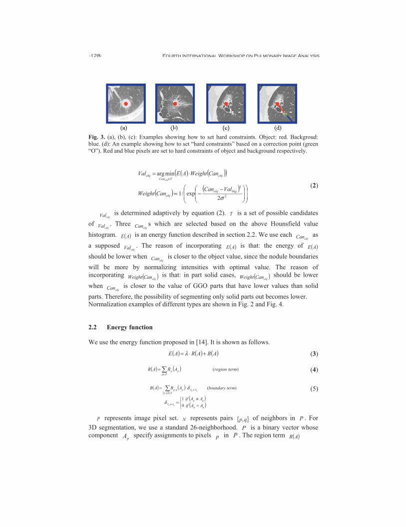
Fig. 3. (a), (b), (c): Examples showing how to set hard constraints. Object: red. Backgroud: blue. (d): An example showing how to set “hard constraints” based on a correction point (green “O”). Red and blue pixels are set to hard constraints of object and background respectively.

( ) ( )( )

( ) ( )��

�

�

��

�

��

��

� −−∝

⋅=∈

2

2

2exp/1

minarg

σbkgobj

obj

objTCan

obj

ValCanCanWeight

CanWeightAEValobj

(2)

objVal is determined adaptively by equation (2). T is a set of possible candidates

of objVal . Three

objCan s which are selected based on the above Hounsfield value histogram. ( )AE is an energy function described in section 2.2. We use each

objCan as a supposed

objVal . The reason of incorporating ( )AE is that: the energy of ( )AE should be lower when

objCan is closer to the object value, since the nodule boundaries will be more by normalizing intensities with optimal value. The reason of incorporating ( )objCanWeight is that: in part solid cases, ( )objCanWeight should be lower when

objCan is closer to the value of GGO parts that have lower values than solid parts. Therefore, the possibility of segmenting only solid parts out becomes lower. Normalization examples of different types are shown in Fig. 2 and Fig. 4.

2.2 Energy function

We use the energy function proposed in [14]. It is shown as follows.

( ) ( ) ( )ABARAE +⋅= λ (3)

( ) ( ) )( termregionARARPp

pp�∈

= (4)

( ) ( ){ }

( )( )

�

=≠

=

⋅=

≠

∈≠�

qp

qpAA

NqpAApqp

AAifAAif

termboundaryABAB

qp

qp

01

)(,

,

δ

δ (5)

P represents image pixel set. N represents pairs { }qp, of neighbors in P . For 3D segmentation, we use a standard 26-neighborhood. P is a binary vector whose component pA specify assignments to pixels p in P . The region term ( )AR


Fig. 4. Comparison results. (a) Cropped image. (b) Normalized intensity. (c) Inverse magnitude of Sobel filter. (d) Result of (c). (e) ( )pAdaScore . (f) Result of (e). assumes that the individual penalties for assigning pixel p to object and background. The boundary term ( )AB comprises the boundary properties of segmentation.

qpB ,

should be small if boundary possibility between p and q is high.

2.2.1 Region Energy

Generally, the region energy is defined as follows. pI and

qI represent intensities.

( ) ( )( ) ( )bkgIbkgR

objIobjR

pp

pp

|Prln

|Prln

−=

−= (6)

However, because of cavities inside and partial volume effects, it is impossible to calculate object intensity likelihood correctly. Therefore, we only set “hard constraints” [14] to pixels which are regarded soundly as object or background. Examples are shown in Fig. 3.

( )

( )

{ }�

∈∈+=� =

=

�

=

NqpqqpPp

p

p

BK

OtherwisepifK

bkgR

OtherwiseROIofperimetertheonispifK

objR

,:,max1

,0SeedPoint,

,0,

(7)

2.2.2 Boundary Energy

( )��

��

� −−∝ 2

2

, 2exp

σqp

qp

IIB

(8)

Generally, the boundary energy is calculated by equation (8). However, we calculate the boundary energy as follows because: 1) nodule size is unknown in advance; 2) segmentation result should be sphere-like; 3) intensity difference can not represent nodule boundaries of different types well.


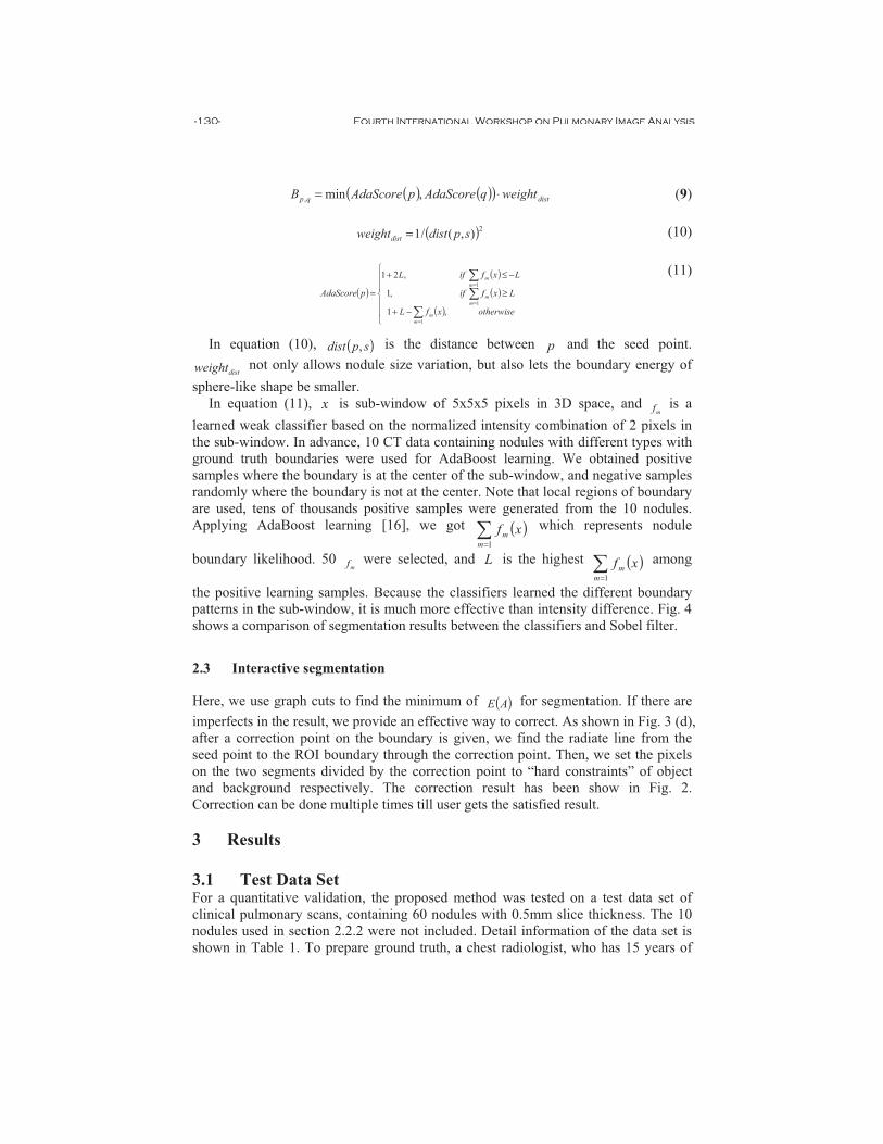
( ) ( )( ) distqp weightqAdaScorepAdaScoreB ⋅= ,min, (9)

( )2),(/1 spdistweightdist = (10)

( )( )( )

( )��

��

�

−+

≥

−≤+

=

��

=

=

=

otherwisexfL

Lxfif

LxfifL

pAdaScore

mm

mm

mm

,1

,1

,21

1

1

1

(11)

In equation (10), ( )spdist , is the distance between p and the seed point.

distweight not only allows nodule size variation, but also lets the boundary energy of sphere-like shape be smaller.

In equation (11), x is sub-window of 5x5x5 pixels in 3D space, and mf is a

learned weak classifier based on the normalized intensity combination of 2 pixels in the sub-window. In advance, 10 CT data containing nodules with different types with ground truth boundaries were used for AdaBoost learning. We obtained positive samples where the boundary is at the center of the sub-window, and negative samples randomly where the boundary is not at the center. Note that local regions of boundary are used, tens of thousands positive samples were generated from the 10 nodules. Applying AdaBoost learning [16], we got ( )�

=1mm xf which represents nodule

boundary likelihood. 50 mf were selected, and L is the highest ( )�

=1mm xf among

the positive learning samples. Because the classifiers learned the different boundary patterns in the sub-window, it is much more effective than intensity difference. Fig. 4 shows a comparison of segmentation results between the classifiers and Sobel filter.

2.3 Interactive segmentation

Here, we use graph cuts to find the minimum of ( )AE for segmentation. If there are imperfects in the result, we provide an effective way to correct. As shown in Fig. 3 (d), after a correction point on the boundary is given, we find the radiate line from the seed point to the ROI boundary through the correction point. Then, we set the pixels on the two segments divided by the correction point to “hard constraints” of object and background respectively. The correction result has been show in Fig. 2. Correction can be done multiple times till user gets the satisfied result. 3 Results

3.1 Test Data Set For a quantitative validation, the proposed method was tested on a test data set of clinical pulmonary scans, containing 60 nodules with 0.5mm slice thickness. The 10 nodules used in section 2.2.2 were not included. Detail information of the data set is shown in Table 1. To prepare ground truth, a chest radiologist, who has 15 years of


experience with the interpretation of thoracic CT images, manually drew the boundaries of each nodule on all 2D axial images.

Table 1. Detail information of the test data set.

Subgroup N / N Internal opacity Solid / Part solid & GGO 33 / 27 Adherence to vessels & pleura None / Present 20 / 40 Diameter(mm) �2 / >2 24 / 36

3.2 Quantitative Evaluation

Experiments of our interactive segmentation evaluate the segmentation results on the test data set. Segmentation results can be corrected several times until the satisfied result is got. Frequency of correction was that: 1) 0 times: 46%; 2) 1-2times: 31%; 3) >2times: 23%. The largest correction times required in the experiments was 4. Nodules adherent to vessels and pleura are prone to have large correction times. Average processing time for segmenting a nodule once is about 2~3 seconds on a quad-core 2.8 GHz PC. And time with and without correction points are almost the same.

Dice’s coefficient (R) between each segmented nodule and the ground truth nodule is calculated as follows:

YXYX

R+∩

=2 (12)

where X and Y are the segmented nodule region and the ground truth respectively. The notation |.| stands for the total number of voxels in the regions.

Fig. 5. Dice's coefficients. Blue dots: solid. Pink dots: part solid & GGO nodules.

Dice's coefficient for nodules (solid / part solid & GGO nodules)

00.10.20.30.40.50.60.70.80.9

1

0 10 20 30 40 50 60 70

Nodule number

coef

ficie

nt (R

)


Fig. 6. Dice's coefficient. Blue dots: solitary. Pink dots: adherent to vessels & pleura.

The mean Dice’s coefficient is 0.85. Fig. 5 shows that, coefficients between solid and part solid & GGO are almost the same. This demonstrates that, our method makes the segmentation robust for both solid and part solid & GGO. Fig. 6 shows that, coefficients between solitary and non-solitary are almost the same. This demonstrates the effectiveness of the interactive correction. Fig. 7 shows some 3D segmentation results. In [6], the mean coefficient for GGO was 0.63 and no effective correction method was proposed. Our method has a much higher Dice’s mean coefficient (0.84) for GGO.

Fig. 7. 3D segmentation results shown by 3 axial images. Column 1,4,6: cropped images. Column 2,5,7: ground truth. Column 3,6,9: results of our method. Row 1: result without correction, R=0.90. Row 2: result without correction, R=0.89. Row 3: result without correction, R=0.83. Row 4: result with 3 correction points, R=0.81.

Dice's coefficient for nodules (solitary / adherent to vessels & pleura)

00.10.20.30.40.50.60.70.80.9

1

0 10 20 30 40 50 60 70

Nodule number

coef

ficie

nt (R

)


4 Conclusion

This paper proposed a novel interactive lung nodule segmentation method using AdaBoost and graph cuts. There are three contributions in this work. The first one is that object intensity is estimated based on energy function. The second one is that boundary energy of graph cuts is determined by AdaBoost. The third one is that an effective correction way is provided. The first and second contributions improve segmentation accuracy a lot, and the third one provides a novel effective way to segment difficult nodules satisfactorily. Because our method is based on AdaBoost and graph cuts, it is generic and can be applied to other tumor segmentation. References

1. Revel, M., et al.: Software Volumetric Evaluation of Doubling Times for Differentiating Benign Versus Malignant Pulmonary Nodules. In: AJR 2006; 187: pp.135-142, (2006)

2. Winer-Muram, H., et al.: Volumetric Growth Rate of Stage I Lung Cancer prior to Treatment: Serial CT Scanning. In: Radiology, pp. 798-805, (2002)

3. Henschke, C., et al.: CT Screening for Lung Cancer Frequency and Significance of Part-Solid and Nonsolid Nodules. In: AJR, pp. 1053-1057, (2002)

4. Okada, K., Comaniciu, D., Krishnan, A.: Robust Anisotropic Gaussian Fitting for Volumetric Characterization of Pulmonary Nodules in Multislice CT. In: IEEE Trans. Medical Imaging, 24(3): 409-423 (2005)

5. Ye, X., Siddique, M., Douiri, A., Beddoe, G., Slabaugh, G.: Graph-cut based automatic segmentation of lung nodules using shape, intensity and spatial features. In: in Proceedings of the 2nd International Workshop on Pulmonary Image Analysis, Held in Conjunction with MICCAI 2009, (2009)

6. Ye, X., Beddoe, G., Slabaugh, G.: Research Article Automatic Graph Cut Segmentation of Lesions in CT Using Mean Shift Superpixels. In: International Journal of Biomedical Imaging, Volume 2010, Article ID 983963, (2010)

7. Dehmeshki, J., Amin, H., Valdivieso, M., Ye, X.: Segmentation of pulmonary nodules in thoracic CT scans: a region growing approach. IEEE Transactions on Medical Imaging, vol. 27, no. 4, pp. 467–480, (2008)

8. Zheng, Y., Kambhamettu, C., Bauer, T., Steiner, K.: Estimation of ground-glass opacity measurement in CT lung images. In: MICCAI 2008, pp. 238–245, (2008)

9. Makrogiannis, S., Bhotika, R., Miller, J., Skinner, J., Vass, M.: Nonparametric Intensity Priors for Level Set Segmentation of Low Contrast Structures. In: MICCAI2009, pp. 239-246, (2009)

10. Ochs, R., et al: Automated classification of lung bronchovascular anatomy in CT using AdaBoost. In: Medical Image Analysis, Volume 11, Issue 3, June 2007, pp. 315-324, (2007)

11. Wu, D., et al.: Stratified learning of local anatomical context for lung nodules in CT images. In: CVPR, pp. 2791-2798, (2010)

12. Li, Y., Hara, S., Ito, W., Shimura, K.: A machine learning approach for interactive lesion segmentation. In: Proceedings of SPIE Medical Imaging, Vol. 6512, (2007)

13. Boykov, Y., Kolmogorov, V.: An Experimental Comparison of Min-Cut/Max-Flow Algorithms for Energy Minimization in Vision. IEEE transactions on Pattern Analysis and Machine Intelligence, vol. 26, no. 9, pp. 1124-1137, Sept. (2004)

14. Boykov, Y., Funka-Lea, G.: Graph Cuts and Efficient N-D Image Segmentation. In: International Journal of Computer Vision (IJCV), vol. 70, no. 2, pp. 109-131, (2006)

15. Schapire, R. E., Singer, Y.: Improved boosting algorithms using confidence-rated predictions. In: Machine Learning, 37:297–336, (1999)

16. Friedman, J., et al: Additive logistic regression: a statistical view of boosting. In: Annals of Statistics, 28(2), 337–407, (2000)


interactive segmentation of lung nodules using … department of radiology, nagoya university...

Documents