interactive simulation of rigid body dynamics in … 2012/ m.-p. cani, f. ganovelli star – state...

EUROGRAPHICS 2012/ M.-P. Cani, F. Ganovelli STAR – State of The Art Report

Interactive Simulation of Rigid Body Dynamics in ComputerGraphics

Jan Bender1, Kenny Erleben2, Jeff Trinkle3 and Erwin Coumans4

1Graduate School CE, TU Darmstadt, Germany2Department of Computer Science, University of Copenhagen, Denmark

3Department of Computer Science, Rensselaer Polytechnic Institute, USA4Advanced Micro Devices, Inc., USA

AbstractInteractive rigid body simulation is an important part of many modern computer tools. No authoring tool nor agame engine can do without. The high performance computer tools open up new possibilities for changing howdesigners, engineers, modelers and animators work with their design problems.This paper is a self contained state-of-the-art report on the physics, the models, the numerical methods and thealgorithms used in interactive rigid body simulation all of which has evolved and matured over the past 20 years.The paper covers applications and the usage of interactive rigid body simulation.Besides the mathematical and theoretical details that this paper communicates in a pedagogical manner the papersurveys common practice and reflects on applications of interactive rigid body simulation. The grand merger ofinteractive and off-line simulation methods is imminent, multi-core is everyman’s property. These observationspose future challenges for research which we reflect on. In perspective several avenues for possible future workis touched upon such as more descriptive models and contact point generation problems. This paper is not only astake in the sand on what has been done, it also seeks to give newcomers practical hands on advices and reflectionsthat can give experienced researchers afterthought for the future.

Keywords: Rigid Body Dynamics, Contact Mechanics, Articulated Bodies, Jointed Mechanisms, Contact PointGeneration, Iterative Methods.

Categories and Subject Descriptors (according to ACM CCS): Computer Graphics [I.3.5]: Computational Geometryand Object Modeling—Physically-based modeling; Computer Graphics [I.3.7]: Three-Dimensional Graphics andRealism—Animation; Mathematics of Computing [G.1.6]: Numerical Analysis—Nonlinear programming

1. Motivation and Perspective on Interactive RigidBody Simulation

Rigid body dynamics simulation is an integral and importantpart of many modern computer tools in a wide range of ap-plication areas like computer games, animation software fordigital production including special effects in film and ani-mation movies, robotics validation, virtual prototyping, andtraining simulators just to mention a few.

In this paper we focus on interactive rigid body dynamicssimulation a subfield that has evolved rapidly over the past10 years and moved the frontier of run-time simulation toapplications in areas where off-line simulation only recentlywere possible. As a consequence this changes the computer

tools humans use and has great social economical impact onsociety as a whole.

The term “interactive” implies a loop closed around a hu-man and simulation tool. For applications like games wherethe feedback is simply animation on a screen, a reasonablegoal is that the simulation deliver 60 frames per second (fps).For haptic rendering, the simulation would be part of a feed-back loop running at 1000Hz, where this rate is needed todisplay realistic forces to the user.

In this state-of-the-art paper we will cover the importantpast 20 years of work on interactive rigid body simulationsince the last state-of-the-art report [Bar93b] on the subject.Rigid body dynamics has a long history in computer graph-

© The Eurographics Association 2012.

J. Bender et al. / Interactive Rigid Body Simulation

Figure 1: Interactive rigid body simulations require the ef-ficient simulation of joints, motors, collisions and contactswith friction.

ics for more than 30 years [AG85, MW88, Hah88, Bar89,BBZ91] and a wealth of work exists on the topic. As earlyas 1993 there were written state-of-the-art reports on thesubject [Bar93b]. In his 93 STAR paper Baraff discussedpenalty based methods and constraint based methods beingan acceleration-level linear complementarity problem for-mulation. He did not cover many details on solving the linearcomplementarity problem. Not until 94 where Baraff pub-lished his version of a direct method based on pivoting wasit feasible to compute solutions for Baraff’s complementar-ity problem formulation. For years the 94 Baraff solutionwas the de-facto standard method of rigid body dynamicschoice in both Maya and Open Dynamics Engine [Smi00].However, the solution only remained interactive for smallsized configurations (below 100 interacting objects or so).When the number of interacting objects increased the com-putational cost quickly made simulations last for hours andthe acceleration-level formulation caused problems too withexistence of solutions and uniqueness. Besides, solutionsfound by his algorithm did not always satisfy the static fric-tion constraints. In the following years after Baraff’s 1994results, the impulse based paradigm was revisited by Mir-tich in 96 [Mir96b] and become a strong competitor whenconcerning interactive simulation. Soon the interactive sim-ulation community moved onto iterative methods and veloc-ity level formulations, eventually evolving into the technol-ogy one finds today in engines such as Bullet [Cou05] andOpen Dynamics Engine. As of this writing interactive sim-ulation on single core CPUs with several 1000 and up to10000 interacting objects are feasible. Multi-core and GPUworks even go far beyond these limits. Even today much ac-tive cross-disciplinary work is ongoing on different contactformulations and iterative solvers taking in people not onlyfrom the field of computer graphics, but also from appliedmath, contact mechanics, robotics and more. Looking be-yond contact problems, one also finds that simulation meth-

Figure 2: The simulation loop provides a coarse descriptionof data flow and processes in a rigid body simulator.

ods for articulated bodies have also undergone rapid devel-opment. In computer graphics, the reduced coordinate for-mulations have won much recognition as being superior forinteractive rag-doll simulations.

1.1. The Anatomy and Physiology of a Rigid BodySimulator

A rigid body simulator is a complex and large piece of soft-ware. Traditionally it has been broken down into smallerwell-defined pieces that each are responsible for solving asimpler single task. All pieces are tied together by a simula-tion loop shown in Figure 2. The loop begins with a col-lision detection query to find the contact points betweenthe various bodies. These points are needed to write thephysical laws governing the motions of the bodies, whichare then solved to determine contact forces that provideproper contact friction effects and prevent bodies from inter-penetrating. This phase is termed “contact handling.” Newlyformed contacts imply collisions, which are accompaniedby impulsive forces (i.e., forces with infinite magnitudesover infinitesimal time periods). Impulsive forces cause in-stantaneous changes in the body velocities and so are oftenhandled separately from pre-existing resting contacts. Onerefers to this as “collision resolving.” After computing allthe contact forces, the positions and velocities of the bodiesare integrated forward in time before a new iteration of thesimulation loop starts. Several iterations of the loop mightbe performed before a frame is rendered.

In order to derive the correct physical laws for the scene,all contacts between bodies must be found. If there are nbodies, then there are O(n2) pairs of bodies to test for col-lisions. To avoid collision detection becoming a computa-tional bottleneck, it is broken into phases. In the first phase,called the “broad phase”, bodies are approximated by simplegeometric primitives for which distance computations arevery fast (see Figure 3). For example, each body is replacedby the smallest sphere that completely contains it. If thespheres covering two bodies do not overlap, then neither dothe actual bodies. The broad phase culling happens in globalworld coordinates. If the individual bodies are complex and



Figure 3: A modular phase description of the sub tasks ofa rigid body simulator helps decomposing a large complexsystem into simpler components.

consist of many parts an additional stage called “mid phase”is used to cull parts in local body space. The culling is typ-ically performed using bounding volume hierarchies. In the“narrow phase” the detailed geometries of bodies are used tofind the precise body features in contact and the location ofthe contact points. However, this expensive operation mustbe done only for the pairs of bodies with overlapping ap-proximations. The narrow phase is often mixed with the midphase for performance reasons. Note that some narrow phasealgorithms do not return all the required contact information,in which case a separate contact point generation algorithmcan be applied (see section 6.3)

1.2. The Quest for Robustness, Accuracy, andPerformance

The recent trend in interactive rigid body simulation has fo-cused on delivering larger and larger simulations of rigidbodies or creating simulation methods that can deliver re-sults faster. Thus, the old saying bigger and faster is betteris very descriptive for many past works in the field of inter-active rigid body simulation. The need for bigger and fasteris motivated by rigid body simulators being used in for in-stance digital production. It looks more interesting to havea pile of skeleton skulls in a movie than having a hand fullof cubes and spheres. Thus, the need in production for cre-ating interesting motion requires more complex simulationscenarios.

The well known tradeoff between accuracy and perfor-mance is an inherent property of interactive rigid body sim-ulation. Many applications enforce a performance constraintwhich leaves too little time for computing accurate solutions.Thus, one must often balance accuracy and stability proper-ties to meet the performance constraint.

Robustness is another desirable numerical trait of a simu-lator. The motivation for this is often caused by having a hu-man being (or the real world in case of robotics) interacting

with a simulator. This may be the cause for much pain andfrustrations as humans have a tendency to be unpredictable.

In summary, the holy grail of interactive rigid body sim-ulation is extremely fast and robust simulation methods thatcan deal gracefully with large scale complex simulation sce-narios under hard performance constraints.

1.3. Application Areas of Interactive Rigid BodySimulation

The maturing technology makes it possible to use rigid bodysimulators as sub-parts in larger systems. For instance intime critical scenarios like tracking humans or maneuveringa robot, a simulator can be used as a prediction tool.

From a digital design viewpoint, one may define a spec-trum of technology. At one end of the spectrum one findsoff-line simulators that may take hours or days to computeresults, but on the other hand they deliver high quality re-sults. For movie production several such computer graph-ics simulation methods have been presented [Bar94,GBF03,KSJP08]. At the other end of the spectrum one finds the fastrun-time simulators capable of delivering plausible resultsvery fast. This kind of simulator often originates from gamephysics. One example is Bullet. At the middle of the spec-trum one finds moderately fast simulators that may deliverhigh fidelity results. These are very suitable for testing de-sign ideas or training.

In general different application areas have different needsin regards to performance/quality trade-offs and accuracy.With this in mind we will discuss a few application areas inthe next four subsections.

1.3.1. Entertainment for Games and Movies

For games and movies rigid body simulation has to be plau-sible rather than physically realistic. For games, the simu-lation needs to be real-time. Simulations for movies do nothave the real-time constraint, but fast simulation methods arealso preferred, since very complex scenarios are simulatedfor special effects and simulation time costs money. There-fore, the development in the two areas go in the same direc-tion. Iterative constraint solving methods are popular in bothareas.

Many games using 2D and 3D graphics rely on a rigidbody dynamics engine to deal with collision detection andcollision response. In some cases the motion of the objectsis fully driven by rigid body dynamics, for example the gameAngry Birds,using the Box2D physics engine or a 3D Jengagame. More commonly, object motion is customized in anon-physical way to a certain degree, to favor a satisfyinggame playing experience over physical realism. This intro-duces the challenge of interaction between rigid bodies andkinematically animated objects. Kinematically animated ob-jects can be represented as rigid bodies with infinite mass,



so that the interaction is one way. The influence from rigidbody to kinematically animated objects is often scripted in anon-physical way.

With increasing CPU budgets, there is growing interest inusing more realistic, higher quality simulation. In particularthe combination of rag-doll simulation, animation, inversekinematics and control requires better methods. It requiresconstraint solvers that can deal with very stiff systems andstrong motors that can deal with the large change in veloc-ity. Several game and movie studios are using Featherstone’sarticulated body method to simulate rag-dolls.

Destruction and fracture of objects can generate a lot ofdynamic rigid bodies, and to handle them, games use multi-core CPUs or offload the rigid body simulation onto GPUs.

1.3.2. Interactive Digital Prototyping

Interactive virtual prototyping can be an important computertool for verifying a design idea or as a pre-processing toolto tune parameters for more computational expensive sim-ulation tools. CEA LIST [CEA11], CMLabs, robot simula-tors Webots, Gazebo, or Microsoft robotics developer stu-dio [KP09,Cyb09,Mic09] are a few examples of many suchtools. The main goal is to reduce the time to market andthereby lower overall production costs. A secondary goal isdevelopment of better products of higher quality.

Interactive prototyping has been motivated by the compu-tational fast technology that has evolved in the gaming andmovie industries. The instant feedback that can be obtainedfrom such simulations is attractive for rapid iterative proto-typing. However, although interactivity is attractive, one cannot compromise the physical correctness too much. Thus,plausible simulation [BHW96] may not be good enough fortrusting a virtual design. A current trend is seen where inter-active simulation tools are improved for accuracy and movedinto engineering tools [Stu08, TNA08, TNA∗10, CA09].

Even the European space agency (ESA) is using PhysXfor verification of the Mars sample rover for the ExoMarsProgramme to investigate the Martian environment [KK11].

1.3.3. Robotics

The main goal of the field of robotics is the developmentof intelligent man-made physical systems that can safelyand efficiently accomplish a wide range of tasks that aidthe achievement of human societal goals. Tasks that areparticularly difficult, dangerous or boring are good candi-dates for robotic methods, e.g., assembly in clean-room envi-ronments, extra-terrestrial exploration, radioactive materialshandling, and laparoscopic surgery. In addition, methods forrobotics are increasingly being applied in the developmentof new generations of active prosthetic devices, includinghands, arms and legs. The most challenging of these tasksmost directly related to this paper are those that cannot be

accomplished without (possibly) intermittent contact, suchas walking, grasping and assembly.

Until now, robot manipulation tasks involving contacthave been limited to those which could be accomplished bycostly design of a workcell or could be conducted via tele-operation. The ultimate goal, however, is to endow robotswith an understanding of contact mechanics and task dy-namics, so they can reason about contact tasks, automati-cally plan and execute them, and enhance their manipulationskills through experience. The fundamental missing compo-nent has been fast, physical simulation tools that accuratelymodel effects such as stick-slip friction, flexibility, and dy-namics. Dynamics is important for robots to perform manip-ulation tasks quickly or to allow it to run over uneven terrain.Physical simulation today has matured to the point where itcan be integrated into algorithms for robot design, task plan-ning, state-estimation and control. As a result, the number ofrobotic solutions to problems involving contact is poised toexperience a major acceleration.

1.3.4. Industrial and Training Simulators

Computer simulators are cheap and risk free ways to trainpeople to handle heavy equipment in critical situations underlarge stress. Examples include large forest machines as wellas bulldozers to cable simulations in tug boats and maneuverbelt vehicles [SL08]. Driving simulators are another goodexample [Uni11, INR11]. The simulators in this field needto be responsive as well as accurate enough to give properpredictions of the virtual equipment being handled. This issimilar to interactive virtual prototyping. In fact in our viewit is mostly the purpose that distinguishes the two, one isdesign the other is training.

The driving simulators are very specialized and includemany aspects of virtual reality. The largest and most com-plex simulator, National Advanced Driving Simulator(NADS), costs in the order of $54 million. In contrast,Gazebo is free software and commercial software such asVortex [CM 11] or Algoryx [Alg11]) are cheap in compari-son with NADS.

2. A Quick Primer

Rigid body simulation is analogous to the numerical solu-tion of nonlinear ordinary differential equations for whichclosed-form solutions do not exist. Assume time t is the in-dependent variable. Given a time period of interest [t0, tN ],driving inputs, and the initial state of the system, the dif-ferential equations (the instantaneous-time model) are dis-cretized in time to yield an approximate discrete-time model,typically in the form of a system of (state-dependent) al-gebraic equations and inequalities. The discrete-time modelis formulated and solved at each time of interest, (t0, .., tN ).In rigid body simulation, one begins with the Newton-Euler(differential) equations, which describes the dynamic motion



of the bodies without contact. These differential equationsare then augmented with three types of conditions: nonpene-tration constraints that prevent the bodies from overlapping,a friction model that requires contact forces to remain withintheir friction cones, and complementarity (or variational in-equality) constraints that enforce certain disjunctive relation-ships among the variables. These relationships enforce criti-cally important physical effects; for example, a contact forcemust become zero if two bodies separate and if bodies aresliding on one another, the friction force acts in the direc-tion that will most quickly halt the sliding. Putting all thesecomponents together yields the instantaneous-time model,as a system of differential algebraic equations and inequali-ties that can be reformulated as a differential nonlinear com-plementarity problem (dNCP). The dNCP cannot be solvedin closed form or directly, so instead, one discretizes it intime, thereby producing a sequence of NCPs whose solu-tions approximate the state and contact force trajectories ofthe system. In the ideal case, the discrete trajectories pro-duced in this process will converge trajectories of the orig-inal instantaneous-time model. Computing a discrete-timesolution requires one to consider possible reformulations ofthe NCPs and a choice of solution method. There are manyoptions for instance reformulation as nonsmooth equationusing Fischer-Burmeister function or proximal point map-pings etc.

2.1. Classical Mechanics

Simulation of the motion of a system of rigid bodies is basedon a famous system of differential equations, the Newton-Euler equations, which can be derived from Newton’s lawsand other basic concepts from classical mechanics:

• Newton’s 1st law: The velocity of a body remains un-changed unless acted upon by a force.• Newton’s 2nd law: The time rate of change of momentum

of a body is equal to the applied force.• Newton’s 3rd law: For every force there is an equal and

opposite force.

Two important implications of Newton’s laws when appliedto rigid body dynamics are: (from the first law) the equationsapply only when the bodies are observed from an inertial(non-accelerating) coordinate frame and (from the third law)at a contact point between two touching bodies, the forceapplied from one body onto the second is equal in mag-nitude, opposite in direction, and collinear with the forceapplied by the second onto the first. Applying these twoimplications to Newton’s second law gives rise to differen-tial equations of motion. While the second law actually ap-plies only to particles, Euler was kind enough to extend itto the case of rigid bodies by viewing them as collectionsof infinite numbers of particles and applying a bit of calcu-lus [GPS02, ESHD05]. This is why the equations of motionare known as the Newton-Euler equations.

N

Bx

vω

Fτg

Figure 4: Illustration of a spatial rigid body showing thebody frame B and inertial frame N as well as notationfor positions, velocities and forces.

Before presenting the Newton-Euler equations, we needto introduce a number of concepts from classical mechanics.Figure 4 shows a rigid body in space, moving with transla-tional velocity v and rotational velocity ω, while being actedupon by an applied force F and moment τ (also known as atorque).

2.1.1. Rigid Bodies

A rigid body is an idealized solid object for which the dis-tance between every pair of points on the object will neverchange, even if huge forces are applied. A rigid body hasmass m, which is distributed over its volume. The centroidof this distribution (marked by the circle with two black-ened quarters) is called the center of mass. To compute ro-tational motions, the mass distribution is key. This is cap-tured in a 3×3 matrix known as the mass (or inertia) matrixI ∈ R(3×3). It is symmetric and positive definite matrix withelements known as moments of inertia and products of iner-tia, which are integrals of certain functions over the volumeof the body [Mei70]. When the integrals are computed in abody-fixed frame, the mass matrix is constant and will bedenoted by Ibody. The most convenient body-fixed frame forsimulation is one with its origin at the center of mass andaxes oriented such that Ibody is diagonal. When computed inthe inertial frame, the mass matrix is time varying and willbe denoted by I.

2.1.2. Rigid Body Kinematics

The body’s position in the inertial (or world) frame is givenby the vector x ∈ R3, from the origin of the inertial frameN fixed in the world to the origin of the frame B fixedin the body. Note that since three independent numbers areneeded to specify the location of the center of mass, a rigidbody has three translational degrees of freedom.

The orientation of a rigid body is defined as the orien-tation of the body-fixed frame with respect to the inertialframe. While many representations of orientation exist, herewe use rotation matrices R ∈ R3×3 and unit quaternions



Q ∈ H. Rotation matrices are members of the class of or-thogonal matrices. Denoting the columns by R1, R2, andR3, orthogonal matrices must satisfy: ‖ Ri ‖= 1; i = 1,2,3and RT

i R j = 0; ∀i 6= j; i = 1,2,3; j = 1,2,3. Since the ninenumbers in R must satisfy these six equations, only threenumbers can be freely chosen. In other words, a rigid bodyhas three rotational degrees of freedom. A unit quaternionis four numbers [Qs, Qx, Qy, Qz], constrained so that thesum of their squares is one. The fourth element can be com-puted in terms of the other three, and this redundancy servesas additional confirmation that orientation has three degreesof freedom. Considering translation and rotation together, arigid body has six degrees of freedom.

The rotational velocity ω ∈ R3 (also known as, angularvelocity) of a body can be thought of as vector whose di-rection identifies a line about which all points on the bodyinstantaneously rotate (shown as a red vector with a doublearrowhead in Figure 4). The magnitude determines the rateof rotation. While the rate of rotation may be changing overtime, at each instant, every point on a rigid body has exactlythe same rotational velocity. The three elements of ω corre-spond to the three rotational degrees of freedom.

Translational velocity v ∈ R3 (also inaccurately referredto as linear velocity) is an attribute of a point, not a body,because when a body rotates, not all points have the samevelocity (see the red vector with a single arrowhead in Fig-ure 4). However, the velocity of every point can be deter-mined from the velocity of one reference point and the an-gular velocity of the body. In rigid body dynamics, the centerof mass is typically chosen as the reference point.

Next we need velocity kinematic relationships. Kinemat-ics is the study of motion without concern for forces, mo-ments, or body masses. By contrast, dynamics is the study ofhow forces produce motions. Since dynamic motions mustalso be kinematically feasible, kinematics is an essentialbuilding block of dynamics. The particular kinematic rela-tionships needed here relate the time derivatives of positionand orientation variables to the translational and rotationalvelocities.

Let us define q = (x, Q) as the tuple containing the po-sition of the center of mass and the orientation parameters.Note that the length of q is seven if Q is a quaternion (whichis the most common choice). The generalized velocity ofthe body is defined as: u = [vT

ωT ]T ∈ R6. The velocity

kinematic equations for a rigid body relate q to u, whichmay have different numbers of elements. The relationshipbetween the translational quantities is simple: x = v. Thetime rate of change of the rotational parameters Q is a bitmore complicated; it is the product of a Jacobian matrix andthe rotational velocity of the body: Q = G(Q)ω, where thedetails of G(Q) are determined by the orientation represen-tation. In the specific case when Q is a unit quaternion, G(Q)

is defined as follows:

G =12

−Qx −Qy −Qz

Qs Qz −Qy−Qz Qs Qx

Qy −Qx Qs

.Putting the two velocity kinematic relationships togetheryields:

q = Hu (1)

where H =

[13×3 0

0 G

], where 13×3 is the 3-by-3 identity

matrix. Note that when the orientation representation usesmore than three parameters, G is not square, although it hasthe property that GT G = 1, where 1 is the identity matrix ofsize 3.

2.1.3. Constraints

Constraints are equations and inequalities that change theway pairs of bodies are allowed to move relative to one an-other. Since they are kinematic restrictions, they also affectthe dynamics. Constraints do not provide a direct means tocompute the forces that must exist to enforce them. Gener-ally, constraints are functions of generalized position vari-ables, generalized velocities, and their derivatives to any or-der:

C(q1,q2,u1,u2, u1, u2, ..., t) = 0 (2)

or

C(q1,q2,u1,u2, u1, u2, ..., t)≥ 0 (3)

where the subscripts indicate the body. Equality and inequal-ity constraints are referred to as bilateral and unilateral con-straints, respectively.

As an example, consider two rigid spheres of radii r1 andr2 and with centers located at x1 and x2. Consider the con-straint function:

C(x1,x2) = ||x1−x2||− (r1 + r2),

where || · || is the Euclidean two-norm. If C = 0, then the sur-faces of the spheres touch at a single point. If this bilateralconstraint is imposed on the Newton-Euler equations, thenregardless of the speeds of the spheres and the sizes of theforces, the surfaces will always remain in single-point con-tact. Intuitively, for this to happen the constraint force nor-mal to the sphere surfaces can be compressive (the spherespush on each other) or tensile (the spheres pull). By contrast,C≥ 0, then the two spheres may move away from each otherbut never overlap. Correspondingly, the constraint force canonly be compressive.

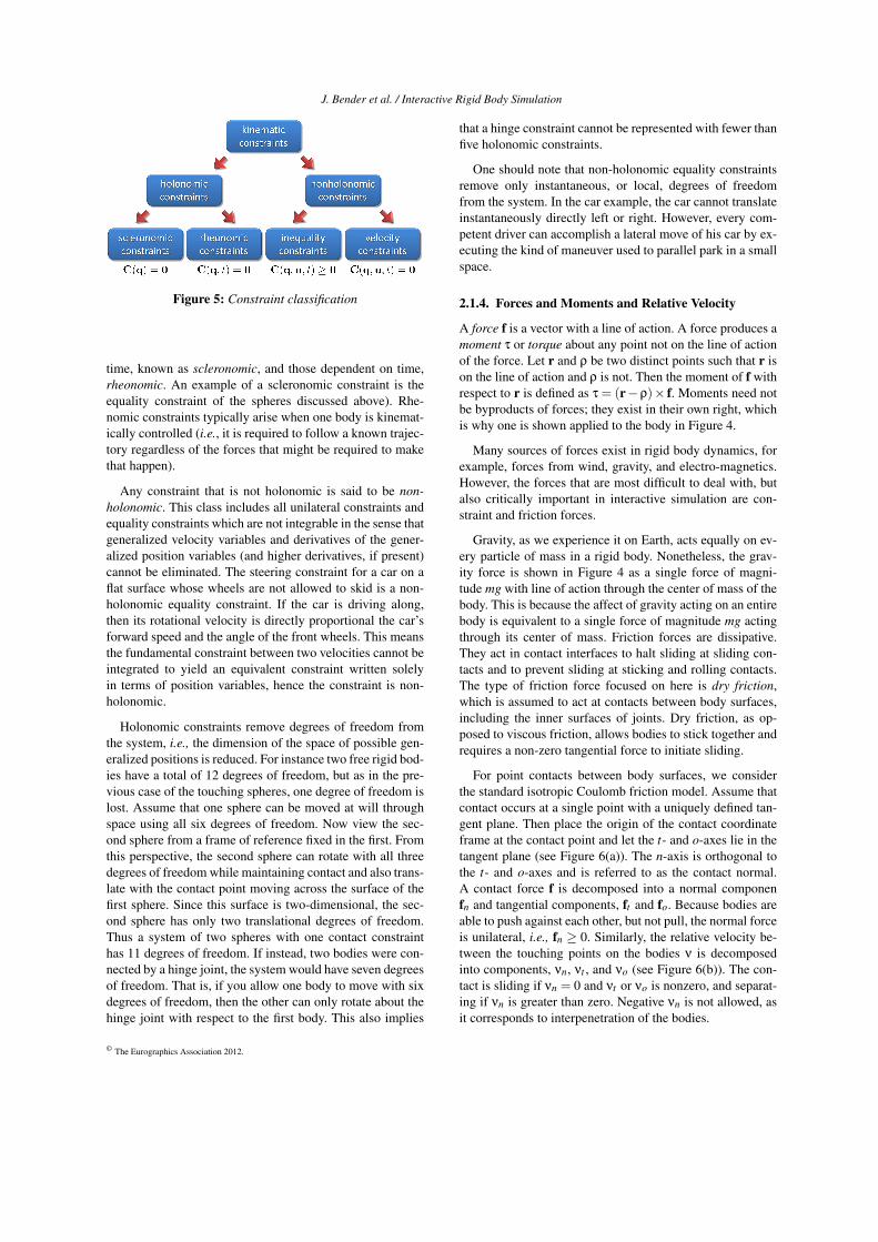
The form of a constraint (see Figure 5) impacts the way inwhich the Newton-Euler equations should be solved. Holo-nomic constraints are those which can be expressed as anequality in terms of only generalized position variables andtime. These are further subdivided into those independent of



Figure 5: Constraint classification

time, known as scleronomic, and those dependent on time,rheonomic. An example of a scleronomic constraint is theequality constraint of the spheres discussed above). Rhe-nomic constraints typically arise when one body is kinemat-ically controlled (i.e., it is required to follow a known trajec-tory regardless of the forces that might be required to makethat happen).

Any constraint that is not holonomic is said to be non-holonomic. This class includes all unilateral constraints andequality constraints which are not integrable in the sense thatgeneralized velocity variables and derivatives of the gener-alized position variables (and higher derivatives, if present)cannot be eliminated. The steering constraint for a car on aflat surface whose wheels are not allowed to skid is a non-holonomic equality constraint. If the car is driving along,then its rotational velocity is directly proportional the car’sforward speed and the angle of the front wheels. This meansthe fundamental constraint between two velocities cannot beintegrated to yield an equivalent constraint written solelyin terms of position variables, hence the constraint is non-holonomic.

Holonomic constraints remove degrees of freedom fromthe system, i.e., the dimension of the space of possible gen-eralized positions is reduced. For instance two free rigid bod-ies have a total of 12 degrees of freedom, but as in the pre-vious case of the touching spheres, one degree of freedom islost. Assume that one sphere can be moved at will throughspace using all six degrees of freedom. Now view the sec-ond sphere from a frame of reference fixed in the first. Fromthis perspective, the second sphere can rotate with all threedegrees of freedom while maintaining contact and also trans-late with the contact point moving across the surface of thefirst sphere. Since this surface is two-dimensional, the sec-ond sphere has only two translational degrees of freedom.Thus a system of two spheres with one contact constrainthas 11 degrees of freedom. If instead, two bodies were con-nected by a hinge joint, the system would have seven degreesof freedom. That is, if you allow one body to move with sixdegrees of freedom, then the other can only rotate about thehinge joint with respect to the first body. This also implies

that a hinge constraint cannot be represented with fewer thanfive holonomic constraints.

One should note that non-holonomic equality constraintsremove only instantaneous, or local, degrees of freedomfrom the system. In the car example, the car cannot translateinstantaneously directly left or right. However, every com-petent driver can accomplish a lateral move of his car by ex-ecuting the kind of maneuver used to parallel park in a smallspace.

2.1.4. Forces and Moments and Relative Velocity

A force f is a vector with a line of action. A force produces amoment τ or torque about any point not on the line of actionof the force. Let r and ρ be two distinct points such that r ison the line of action and ρ is not. Then the moment of f withrespect to r is defined as τ = (r−ρ)× f. Moments need notbe byproducts of forces; they exist in their own right, whichis why one is shown applied to the body in Figure 4.

Many sources of forces exist in rigid body dynamics, forexample, forces from wind, gravity, and electro-magnetics.However, the forces that are most difficult to deal with, butalso critically important in interactive simulation are con-straint and friction forces.

Gravity, as we experience it on Earth, acts equally on ev-ery particle of mass in a rigid body. Nonetheless, the grav-ity force is shown in Figure 4 as a single force of magni-tude mg with line of action through the center of mass of thebody. This is because the affect of gravity acting on an entirebody is equivalent to a single force of magnitude mg actingthrough its center of mass. Friction forces are dissipative.They act in contact interfaces to halt sliding at sliding con-tacts and to prevent sliding at sticking and rolling contacts.The type of friction force focused on here is dry friction,which is assumed to act at contacts between body surfaces,including the inner surfaces of joints. Dry friction, as op-posed to viscous friction, allows bodies to stick together andrequires a non-zero tangential force to initiate sliding.

For point contacts between body surfaces, we considerthe standard isotropic Coulomb friction model. Assume thatcontact occurs at a single point with a uniquely defined tan-gent plane. Then place the origin of the contact coordinateframe at the contact point and let the t- and o-axes lie in thetangent plane (see Figure 6(a)). The n-axis is orthogonal tothe t- and o-axes and is referred to as the contact normal.A contact force f is decomposed into a normal componenfn and tangential components, ft and fo. Because bodies areable to push against each other, but not pull, the normal forceis unilateral, i.e., fn ≥ 0. Similarly, the relative velocity be-tween the touching points on the bodies ν is decomposedinto components, νn, νt , and νo (see Figure 6(b)). The con-tact is sliding if νn = 0 and νt or νo is nonzero, and separat-ing if νn is greater than zero. Negative νn is not allowed, asit corresponds to interpenetration of the bodies.



ft

fo

fn

νt

o

n

(a) A Friction Cone

νt

νo

νn

ν

νf

(b) Contact velocities

Figure 6: The friction cone of a contact and the decomposi-tion of the relative contact velocity.

The Coulomb model has two conditions: first, the net con-tact force must lie in a quadratic friction cone (see the graycone in Figure 6(a)) and second, when the bodies are slip-ping, the friction force must be the one that directly opposessliding. The cone is defined as follows:

F(fn,µ) = µ2f2n− f2

t − f2o ≥ 0, fn ≥ 0 (4)

where µ≥ 0 is the friction coefficient. The friction force thatmaximizes friction dissipation is:

ft = −µfnνt

β(5)

fo = −µfnνo

β(6)

where β =√

ν2t +ν2

o is the sliding speed at the contact (seeFigure 6(b)).

Common variations on this model include using two dif-ferent friction coefficient; one for sticking contact and alower one for sliding. When friction forces are higher inone direction than another, one can replace the circular conewith an elliptical cone. In some simulation schemes the non-linearity of the friction cone causes problems, and so it iseliminated by approximating the cone as a symmetric poly-hedral cone. Finally, to model the fact that contacts betweenreal bodies are actually small patches, the friction cone canbe extended, as done by Contensou, to allow for a fric-tion moment that resists rotation about the contact normal[Con93, TTP01].

A similar model for dry friction acting to resist joint mo-tion will be discussed in section 3.

2.1.5. The Newton-Euler Equations

The Newton-Euler equations are obtained by applying New-ton’s second law twice; once for translational motion andagain for rotational motion. Specifically, the net force F ap-plied to the body is equal to the time rate of change of trans-lational momentum mv (i.e., d

dt (mv) = F) and the net mo-ment τ is equal to the time rate of change of rotational mo-

mentum Iω (i.e., ddt (Iω) = τ). Specializing these equations

to the case of a rigid body (which, by definition, has constantmass) yields:

mv = F (7)

Iω+ω× Iω = τ. (8)

where recall that I is the 3-by-3 inertia matrix and × repre-sents the vector cross product.

The second term on the left side of the rotational equationis called the “gyroscopic force” which arises from the properdifferentiation of the rotational momentum. The rotationalvelocity and mass matrix must both be expressed in the sameframe, which is usually taken as a body-fixed frame (whichis rotating with the body in the inertial frame) or the inertialframe. In a body-fixed frame, Ibody is constant, but ω is avector expressed in a rotating frame, which means that Iω

is also a vector expressed in a rotating frame. The first termrepresents the rate of increase of angular velocity along thevector ω.

One might be tempted to try to eliminate the secondterm by expressing the rotational quantities in the inertialframe and differentiating them there. However this doesnot work, because the inertia matrix expressed in the iner-tial frame I is time-varying, as seen by the following iden-tity I = RIbodyRT . Differentiating inertial frame quantitiesyields an equivalent expression with equivalent complexity.

The Newton-Euler equations contain the net force F andmoment τ. F is simply the vector sum of all forces acting onthe body. τ is the vector sum of the moments of all the forcesand pure moments. One can see from equation (7), that thenet force causes the center of gravity to accelerate in the di-rection of the net force proportional to its magnitude. This istrue independent of the location of the line of action in space.Equation (8) implies that the net moment directly affects therotational velocity of the body, but in a more complicatedway. The gyroscopic moments tend to cause the axis of ro-tation of a rotating rigid body to “precess” about a circularcone.

Simulation of free body motion is done by integratingthe Newton-Euler equations (7,8) and the velocity kinematicequation (1) simultaneously. If there are contacts and joints,then these equations must be augmented with the constraintequations (2,3). If in addition, dry friction exists in contacts,then equations (4,5,6) must be included. The complete sys-tem of differential and algebraic equations and inequalities ischallenging to integrate, but methods to do this robustly havebeen developed over the past 20 years. To push the bound-aries of interactive rigid body dynamics, one must maintainthe current level of solution robustness and greatly increasethe solution speed.

2.1.6. Impulse

When a pair of bodies collides, those bodies, and any otherbodies they are touching, experience very high forces of very



short duration. In the case of ideal rigid bodies, the forcemagnitudes become infinite and the duration becomes in-finitesimal. These forces are referred to as impulsive forcesor shocks. One can see from equation (7), that shocks causeinfinite accelerations, which makes direct numerical integra-tion of the Newton-Euler equations impossible. One way todeal with this problem during simulation is to use a stan-dard integration method up to the time of impact, then usean impulse-momentum law to determine the jump disconti-nuities in the velocities, and finally restart the integrator.

Let [t, t +∆t] be a time step during which a collision oc-curs. Further, define p =

∫ t+∆tt Fdt as the impulse of the

net force and mv as translational momentum. Integratingequation (7) from t to t + ∆t yields m(v(t + ∆t)− v(t)) =∫ t+∆t

t Fdt, which states that impulse of the net applied forceequals the change of translational momentum of the body. Inrigid body collisions, ∆t approaches zero. Taking the limit as∆t goes to zero, one obtains an impulse momentum law thatis applied at the instant of impact to compute post collisionvelocities. Since ∆t goes to zero and the velocities remainfinite, the generalized position of the bodies are fixed duringthe impact. After processing the collision, one has the val-ues of the generalized positions and velocities, which are theneeded initial conditions to restart the integrator. Note thatintegration of the rotational equation (8) yields an impulse-momentum law for determining jump discontinuities in therotational velocities.

Based on impulse-momentum laws, several algebraic col-lision rules have been proposed. Newton’s Hypothesis isstated in terms of the normal component of the relative ve-locity of the colliding points just before and just after colli-sion: v+n =−εv−n , where v−n is relative normal velocity justbefore impact, v+n is the relative normal velocity just afterimpact, and ε ∈ [0,1] is known as the coefficient of restitu-tion. Setting ε to zero yields a perfectly plastic impact (i.e.,an impact with no bounce). Setting this value to 1 yields per-fectly elastic impacts (i.e., no energy is lost).

Poisson’s Hypothesis is similar, but is a function of col-lision impulse rather than the rate of approach. The normalimpulse is divided into two parts, pc

n and prn, which are re-

lated as follows prn = εpc

n, where again ε ∈ [0,1]. Immedi-ately prior to the collision, ν

−n of the impact points is neg-

ative. The compression impulse pcn is defined as the amount

of impulse required to cause the relative normal velocity tobecome zero - just enough to prevent body interpenetrationwith no bounce. The restitution impulse is applied after thecompression impulse to generate bounce (i.e., ν

−n > 0).

The same idea can be applied to frictional collision im-pulses by replacing the normal components of the impulsesand velocities with the tangential components (see for ex-ample [Bra91]). The normal and tangential impact hypothe-ses can be used together to determine the velocity jumpscaused by impacts. While simple and intuitive, this approachcan unfortunately generate energy during oblique collisions.

To prevent such unrealistic outcomes, Stronge developedan energy-based collision law that imposes a condition thatprevents energy generation. Chatterjee and Ruina incorpo-rated Stronge’s energy constraint and recast the collisionlaw in terms of two parameters that are physically mean-ingful [CR98].

3. Models for Interactive Simulation

The laws of physics must be combined into what we term aninstantaneous-time model, which describes the continuousmotions of the rigid bodies. Following this, we discretize thismodel over the time domain to obtain a discrete-time model,which is a sequence of so-called time-stepping subproblems.The subproblems are formulated and numerically solved atevery time step to simulate the system.

In this section, we present generic models for systemswith multiple simultaneous frictional contacts in Section 3.1.The particulars of models for dealing with aspects of reducedcoordinate formulations are covered in Section 3.2.

3.1. Modeling of Simultaneous Frictional Contacts

Here we take a strict approach trying to keep the physicsas correct as possible by only introducing errors of lin-earization and discretization. The model consists of fiveparts: the Newton-Euler equation [Lan86], a kinematic map(to relate time derivatives of configuration parameters totranslational and angular velocity variables), equality con-straints (to model permanent joint connections), normal con-tact conditions (to model intermittent contact behavior),and a dry friction law satisfying the principle of maximumpower dissipation, also known as the principle of maximumwork [Goy89]. These five parts will be explained in detailbelow.

Two types of constraints exist: permanent mechanicaljoints, each represented by a system of equations (five scalarequations in the case of a one-degree-of-freedom joint), andisolated point contacts with well-defined contact normals,each represented by one scalar inequality constraint. Let Band U denote the mutually exclusive sets of bilateral (equal-ity) and unilateral (inequality) contacts:

B = i : contact i is a joint (9)

U = i : contact i is a point contact (10)

where B∪U = 1, ...,nc and nc is the number of contacts.Note that distributed contacts can be approximated arbitrar-ily well by a number of isolated point contacts.

To formulate the equations of motion properly, one needsprecise definitions of contact maintenance, sliding, androlling. It is convenient to partition possible relative mo-tions at each contact into normal and frictional subspaces.Let κCin and κCi f , where κ ∈ b, u, denote signed distance



functions (or gap functions) in the normal and friction sub-space directions at contact i. If two bodies touch at contact i,then κCin = 0. This is always enforced for joints (bCin = 0),which are permanent contacts, but not for unilateral contacts,which can be broken as bodies separate (uCin > 0).

The first time derivatives of the distance functions are therelative contact velocities, κ

νiσ = ddt(

κCiσ)

; κ∈ b, u,σ∈n, f. Note that κ

νin and κνi f are orthogonal subspaces,

where unallowed motions are prevented by body structuresand sliding motions are resisted by friction forces, respec-tively. If a pair of contact points (one on each body at thepoint of touching) are in rolling contact, instantaneously, thedistance between those bodies in the direction of possiblesliding is zero (κ

νi f = 0). If they slip, at least one friction di-rection displacement will become nonzero. For example, thefriction direction of a one-degree-of-freedom joint is in thedirection of motion of the joint. For a unilateral contact withisotropic Coulomb friction, the friction subspace will consistof relative translation in the t- and o-directions. The corre-sponding displacement functions will be denoted by uCit anduCio. Relative rotations are not resisted by body structure orfriction, so they are not included in either subspace.

We now partition all contacts into sliding and rolling sub-sets. At the position level, contact i is sustained if the dis-tance function κCin(q, t); κ ∈ b,u is equal to zero for afinite period of time. However, one cannot distinguish slid-ing from rolling with this position-level condition; one needstime derivatives. The velocity-level set definitions are:

S = i : κCin = 0, κνin = 0, κ

νi f 6= 0 (11)

R = i : κCin = 0, κνin = 0, κ

νi f = 0, (12)

where the sets S andR are mutually exclusive.

We are now in a position to develop the system of equa-tions and inequalities defining the instantaneous-time dy-namic model of a multi-rigid-body system with bilateral andunilateral contacts. Recall the five parts mentioned above.

Newton-Euler Equations: The Newton-Euler equation canbe written as follows:

M(q)u = g(q,u, t), (13)

where M(q) is the generalized mass matrix containing thebody mass properties and g(q,u, t) is the vector of loads,including the gyroscopic moment (the cross-product term inequation (15)). Specifically for the jth rigid body we have:

M j =

[m j13×3 0

0 I j(Q j)

], (14)

g j =

[F j

τ j−ω j× I j(Q j)ω j

], (15)

where 13×3 is the 3-by-3 identity matrix. Recall that I is the3-by-3 inertia matrix, and F j and τ j are the externally ap-plied force and moment. Also note that M is positive definiteand symmetric.

Kinematic Map: The time rate of change of the general-ized coordinates of the bodies q is related to the generalizedvelocities of the bodies u:

q = H(q)u. (16)

where H(q) is the generalized kinematic map. The diagonalblocks H j j are given by equation 1 and off diagonal blocksare zero.

Joint Constraints: Since joints are permanent contacts, ifcontact i is a joint (i.e., i ∈ B), then the vector functionbCin(q, t) = 0 for all time. Stacking the bCin functions forall i ∈ B into the vector bCn(q, t), yields the position-levelconstraint for all joints:

bCn(q, t) = 0. (17)

From a physical perspective, these constraints are main-tained by reaction forces bfin that are unconstrained. Thatis, generalized forces normal or anti-normal to the constraintsurface in the system’s configuration space can be generated.When viewing multibody dynamics from a variational per-spective, these forces are Lagrange multipliers [Lan86].

Normal Contact Constraints: For the unilateral contacts,the scalar functions, uCin(q, t) for all i ∈ U must be non-negative. Stacking all the gap functions into the vectoruCn(q, t) yields the following position-level non-penetrationconstraint:

uCn(q, t)≥ 0. (18)

From a physical perspective, this constraint is maintained bythe normal component of the contact force ufin between thebodies. Again, this force can be viewed as a Lagrange multi-plier, but since the constraint is one-sided, so is the multiplier(i.e., ufin ≥ 0). This means that constraint forces at unilateralcontacts must be compressive or zero. Combining all ufin forall i ∈ U into the vector ufn, we write all normal force con-straints as:

ufn ≥ 0. (19)

There is one more aspect of unilateral contacts that must bemodeled. If contact i is supporting a load (i.e., ufin > 0), thenthe contact must be maintained (i.e., uCin = 0). Conversely,if the contact breaks (i.e., uCin > 0), then the normal com-ponents (and hence the frictional components) of the contactforce must be zero (i.e., ufin = 0). For each contact, at leastone of ufin and uCin must be zero, (i.e., uCin

ufin = 0). Theseconditions are imposed at every contact simultaneously byan orthogonality constraint:

uCn(q, t) · ufn = 0 (20)

where · denotes the vector dot product.

Friction Law: At contact i, the generalized friction forceκfi f can act only in a subset of the unconstrained directionsand must lie within a closed convex limit setFi(

κfin,µi). The



limit set must contain the origin, so that a zero friction forceis possible. Also, typically, the limit set scales linearly withthe normal component of the contact force, thus forming acone of possible contact forces.

When contact i is rolling, the friction force may take onany value within the limit set. However, when the contact issliding, the friction force must be the one within Fi(

κfin,µi)that maximizes the power dissipation. Such models are saidto satisfy the principle of maximum dissipation [Goy89]. Atthe velocity level, maximum dissipation can be expressed asfollows:

κfi f ∈ argmaxf′i f

−κ

νi f ·f′i f : f′i f ∈ Fi(κfin,µi)

(21)

where f′i f is an arbitrary vector in the set Fi(κfin,µi). No-

tice that when this set is strictly convex, then the frictionforce will be unique. For example, under the assumption ofisotropic Coulomb friction at a unilateral contact, the limitset is the disc µ2

iuf2

in− uf2it − uf2

io ≥ 0 and the unique frictionforce is the one directly opposite the relative sliding velocity,(u

νit ,uνio).

Finally, our instantaneous-time dynamic model is the sys-tem of differential algebraic inequalities (DAIs) composedof equations (13,16–21), where the sliding and rolling con-tact sets are defined as in equations (11) and (12) In the cur-rent form, the DAI is difficult to solve. However, as will beshown, it is possible to cast the model as a differential com-plementarity problem [CPS92b,TPSL97], then discretize theresult to form simulation subproblems in the form of non-linear or linear complementarity problems, allowing one toapply well-studied solution algorithms.

Complementarity Problems

The standard nonlinear complementarity problem (NCP) canbe stated as follows:

Definition 1 Nonlinear Complementarity Problem: Given anunknown vector x ∈ Rm and a known vector function y(x) :Rm→ Rm, determine x such that:

0≤ y(x)⊥ x≥ 0, (22)

where ⊥ implies orthogonality (i.e., y(x) · x = 0).

The standard linear complementarity problem (LCP) is aspecial case in which the function y(x) is linear in x:

Definition 2 Linear Complementarity Problem: Given anunknown vector x ∈ Rm, a known fixed matrix A ∈ Rm×m,and a known fixed vector b ∈ Rm, determine x such that:

0≤ Ax+b⊥ x≥ 0. (23)

We adopt the shorthand notation, LCP(A,b).

3.1.1. Complementarity Formulation of theInstantaneous-Time Model

To achieve model formulation as a properly posed comple-mentarity problem, we must write all the conditions (13,16–21) in terms of a common small set of dependent variables.In the current formulation, the dependent variables are posi-tions, velocities, and accelerations. However, by taking theappropriate number of time derivatives, all equations will bewritten in terms of accelerations, thus generating a modelin which all dependent variables are forces and accelera-tions. This transformation will be carried out below in threesteps. First, express the principle of maximum dissipation asa system of equations and inequalities in forces and accel-erations, second, reformulate the Newton-Euler equation toexpose the forces, and third, differentiate the distance func-tions twice with respect to time to expose the accelerations.

Reformulation of maximum dissipation The principle ofmaximum dissipation (21) can be replaced by an equiva-lent system of equations and inequalities by formulating itas an unconstrained optimization problem, and solving it inclosed form. To do this, however, one must choose a spe-cific form of Fi. In this paper, we will demonstrate the so-lution process for isotropic Coulomb friction at a unilateralcontact and apply the result to dry friction of constant maxi-mum magnitude in a one-degree-of-freedom joint. The sameprocedure can be applied to other friction models, includingContensou [TP97, TTP01].

Closed-form solutions of optimization problems cansometimes be found by obtaining a system of equationscorresponding to necessary and sufficient conditions foran optimal solution, then solving them. The most com-mon approach is to augment the objective function withthe constraints multiplied by Lagrange multipliers and thenobtain the equations, known as the Karush-Kuhn-Tucker(KKT) equations, by partial differentiation. To be valid, thesystem must satisfy a regularity condition (also known as,“constraint qualification”). In the case of isotropic Coulombfriction, the system does not satisfy any of the possible reg-ularity conditions at the point of the cone (where ufin = 0),so the method fails.

Fortunately, the more general Fritz-John conditions[MF67] do satisfy a regularity condition everywhere onthe cone. In the case of isotropic Coulomb friction, theaugmented objective function (recall equation (21) is:

− uβi0(

ufituνit +

ufiouνio)+

uβi(µ

2i

uf2in− uf2

it − uf2io), (24)

where uβi and u

βi0 are Lagrange multipliers. To obtain a sys-tem of equations and inequalities equivalent to the maximumdissipation condition (21), one takes partial derivatives withrespect to the unknown friction force components and La-grange multipliers and then imposes the additional condi-tions of the Fritz-John method: u

βi0 ≥ 0 and (uβi0,

uβi) 6=

(0,0). Following the derivation on pages 28-30 of [Ber09],



one arrives at the following system of constraints:

µiufin

uνit +

ufituβi = 0

µiufin

uνio +

ufiouβi = 0

uαi = µ2

iuf2

in− uf2it − uf2

io ≥ 0

0≤ uαi ⊥ u

βi ≥ 0

∀ i ∈ U ∩S, (25)

where uαi is a slack variable for the friction limit set. Note

that uβi =‖

uνi f ‖ at the optimal solution, and represents

the magnitude of the slip velocity at contact i (i.e., uβi =

‖ uνi f ‖=

√uν2

it +uν2

io ). Note that this condition is not writ-ten in terms of accelerations, because at a sliding contact, thefriction force (ufit ,

ufio) can be written in terms of the normalforce and eliminated. For example, in the case of Coulombfriction, equations (5) and (6) are used. Tangential acceler-ation at a contact does not enter unless the contact point isrolling.

If contact i is a one-degree-of-freedom joint, we will as-sume that the maximum magnitude of the dry friction forceis independent of the load in the other five component direc-tions. Thus, the friction limit set for a bilateral joint Fi(µi)will be:

Fi(bfi fmax) =

bfi f :

∣∣∣bfi f

∣∣∣≤ bfi fmax

, ∀ i∈ B∩S (26)

where |·| denotes the absolute value of a scalar and bfi fmax

is the nonnegative maximum magnitude of the generalizedfriction force in joint i.

Notice that this joint friction model is a special case of theresult obtained for Coulomb friction; fix ufinµi to the valueof bfi fmax and remove one of the friction directions, say thet-direction. The result is:

bfiomaxbνio +

bfiobβi = 0

bαi =

bf2iomax −

bf2io ≥ 0

0≤ bαi ⊥ b

βi ≥ 0

∀ i ∈ B. (27)

As before, bβi =‖

bνi f ‖ at an optimal solution.

Contact Constraints in Terms of Accelerations Contactconstraints (unilateral and bilateral) can be written in termsof accelerations through Taylor series expansion of con-straint functions, κCiσ(q, t); κ ∈ b, u; σ ∈ n, f Letq = q+∆q and t = t +∆t where ∆q and ∆t are small per-turbations.

Then the Taylor expansion of one of these scalar displace-ment functions truncated to the quadratic terms is:

κCiσ(q, t) = κCiσ(q, t)

+∂

κCiσ

∂q∆q+

∂κCiσ

∂t∆t

+12

((∆q)T ∂

2κCiσ

∂q2 ∆q+2∂

2κCiσ

∂q∂t∆q∆t +

∂2κCiσ

∂t2 ∆t2

)

Notice that if contact exists at the current values of q and t,then the first term is zero. Dividing the linear terms by ∆t andtaking the limit as ∆t (and ∆q) goes to zero, one obtains therelative velocity, κ

νiσ at the contact. Dividing the quadraticterms by (∆t)2 and taking the limit yields the relative accel-eration κaiσ:

κaiσ = κJiσu+ κkiσ(q,u, t) (28)

where

κJiσ =∂(κCiσ)

∂qH

κkiσ(q,u, t) =∂(κCiσ)

∂q∂H∂t

u+∂

2(κCiσ)

∂q∂tHu+

∂2(κCiσ)

∂t2 ,

where recall that κ is either b or u and σ is either n or f .

Stacking all the quantities above for every unilateral andbilateral contact (as defined in equations (11) and (12)), onearrives at the definitions of κan, κJn, and κkn, which allowsus to express equations (17-20) in terms of accelerations asfollows:

ban = 0. (30)

0≤ ufn ⊥ uan ≥ 0. (31)

The principle of maximum dissipation (21) must be con-sidered further. When contact i is sliding, the solutions ofconditions (25) and (27) produce the correct results (i.e., thefriction force obtains its maximum magnitude and directlyopposes the sliding direction) and, we can use these condi-tions to eliminate κfi f . Also as required, when a contact isrolling, these conditions allow the friction force to lie any-where within the friction limit set. What these conditions donot provide is a mechanism for determining if a rolling con-tact will change to sliding. However, this problem is easilyremedied by replacing the relative velocity variables in equa-tion (21) with the analogous acceleration variables.

µiufin

uait +ufit

uβi = 0

µiufin

uaio +ufio

uβi = 0

uβi = µ2

iuf2

in− uf2it − uf2

io ≥ 0

0≤ uβi ⊥

uβi ≥ 0

∀ i ∈ U ∩R (32)

where uβi =‖

uai f ‖ at the optimal solution, and

bfi fmaxbai f +

bfi fbβi = 0

bβi =

bf2i fmax −

bf2i f ≥ 0

0≤ bβi ⊥

bβi ≥ 0

∀ i ∈ B∩R (33)

where bfi f =∣∣∣bai f

∣∣∣ at the optimal solution.

Exposing the Contact Forces in the Newton-Euler Equa-tion Recall that the vector g(q,u, t) represents the resultantgeneralized forces acting on the bodies, and naturally gener-ated gyroscopic forces. In order to complete the formulationas an NCP, g(q,u, t) is expressed as the sum of the normal



and friction forces at the unilateral and bilateral contacts andall other generalized forces. The Newton-Euler equation be-comes:

M(q)u = uJn(q)T ufn +uJ f (q)

T uf f (34)

+ bJn(q)T bfn +bJ f (q)

T bf f +gext(q,u, t)

where gext(q,u, t) is the resultant of all non-contact forcesand moments applied to the bodies, uf f and bf f are formedby stacking the generalized friction vectors at the unilateraland bilateral contacts respectively, and the matrices κJσ mapcontact forces into a common inertial frame.

3.1.2. A Differential NCP

The instantaneous dynamic model is now complete.

Definition 3 CP1: Equations (16,25,27,30–34) constitute adifferential, nonlinear complementarity problem.

It is known that solutions to CP1 do not always exist(see [TPSL97]), however, if the principle of maximum dis-sipation is relaxed so that friction forces merely need to bedissipative, rather than maximally dissipative, then a solu-tion always exists [PT96]. If one wanted to use this NCP inan integration scheme to simulate the motion of a multibodysystem, the PATH algorithm by Ferris and Munson is themost robust, general purpose NCP solver available [CPN11].One should also note that this NCP can be converted into anapproximate LCP by linearizing the friction cone constraint(see [TPSL97] for details). The LCP then can be solved byLemke’s algorithm [CPS92b], but the solution non-existenceproblem persists unless the maximum dissipation require-ment is relaxed as just stated above.

3.1.3. A Nonlinear Discrete-Time Model

We recommend against applying a integration method to theinstantaneous-time model due the possible non-existence ofcomputable solutions (i.e., a values of the unknown acceler-ations and constraint forces might not exist OR the solutionmight contain infinite values). However, this problem can bealleviated by applying discrete-time derivative approxima-tions to the model over a time step ∆t and then recasting themodel as a time-stepping complementarity problem whoseunknowns are impulses (time integrals of forces) and veloc-ities (time integrals of accelerations). We demonstrate theprocess in this section.

Let ∆t denote a positive step size and t` the current time,for which we have estimates of the configuration q(`) = q(t`)and the generalized velocity u(`) = u(t`) of the system. Ourgoal is to compute configurations q(`+1) = q(t` + ∆t) andvelocities u(`+1) = u(t`+∆t) that lie as close as possible toa solution of the differential NCP, CP1.

In the derivation, we will require estimates of the matricesM, κJσ, and the vector gext, which all vary with the systemconfiguration q. As will be seen, the simplest choice will be

to use their values at q(`), denoted by M(`),κJ(`)σ , and g(`)ext,because that will result in an explicit time-stepping methodwith each step requiring the solution of an NCP, whose onlynonlinearity is the quadratic constraint of the friction cone.Approximating the cone constraint with a polyhedral conewill replace the quadratic constraints with linear ones, andthus will convert the NCP into an LCP, which is typicallyeasier to solve.

In the following section, we discretize the five compo-nents of the instantaneous-time model derived above. Tosimplify our presentation, we choose the simple backwardEuler approximation of the state derivatives, i.e., u(t`+1) ≈(u(`+1)−u(`))/∆t and q(t`+1)≈ (q(`+1)−q(`))/∆t.

Discrete-Time Newton-Euler Equations Applying thebackward Euler approximation to the Newton-Euler equa-tion (34) yields the equation below in which all quantitiesare evaluated at the end of the time step:

M(`+1)(

u(`+1)−u(`))= (uJT

n )(`+1)up(`+1)

n (35)

+(uJTf )

(`+1)up(`+1)f +(bJ

Tn )

(`+1)bp(`+1)n

+(bJTf )

(`+1)bp(`+1)f +(pext)

(`+1),

where the vectors are unknown generalized contact impulsesdefined as p(`+1) = ∆tf(`+1) and pext = ∆tgext is the impulseof the generalized forces applied to the bodies over the timestep.

Discrete-Time Kinematic Map Applying the backwardEuler approximation to the kinematic map (16) gives:

q(`+1)−q(`) = ∆tH(`+1)u(`+1), (36)

which is nonlinear in the unknown system configurationq(`+1). An important issue arises when solving this equationfor q(`+1). The “vector” q(`+1), is NOT a vector; the orienta-tion part of q lives in a curved space, not a vector space. Forexample, when orientation is represented by a unit quater-nion, then quaternion elements of q(`) and q(`+1) must haveunit length, but adding ∆tH(`+1)u(`+1) to q(`) slightly in-creases the length. This problem can be solved simply bynormalizing the quaternion elements of q(`+1) after eachtime step.

Discrete-Time Contact Constraints The contact and jointconstraints given in equations (17,18,20) can be incorpo-rated into the discrete-time framework by replacing the con-figuration variables with their values at time t(`+1). An al-ternative is to expand the functions in a Taylor series andchoose the point of truncation, to control the level of accu-racy and nonlinearity. Denoting κCσ

(q(`), t(`)

)by κC(`)

σ , a



Taylor series expansion is:

κC(`+1)σ = κC(`)

σ +(κJσ)(`)u(`+1)

∆t +∂

κC(`)σ

∂t∆t +H.O.T,

(37)where the hat over the C in denotes an approximation andH.O.T. denotes higher-order terms.

Discrete-Time Normal Contact Constraints Given thatthe discrete time Newton-Euler equations are written interms of unknown impulses, equation (19) should also beconverted to impulses. Since up(`+1)

n = ∆tuf(`+1)n and ∆t is

strictly positive, equation (19) becomes:

up(`+1)n ≥ 0. (38)

Last, for each unilateral contact, we must enforce com-plementarity between the gap function at the end of the timestep and the normal impulse. Inserting the Taylor series ap-proximation into equation (20) yields:

0≤ up(`+1)n ⊥ uC

(`+1)n ≥ 0. (39)

Note that, in general, the right-hand inequality is nonlinearin the unknown u(`+1). However, it can be made linear bytruncating the Taylor series after the linear terms. It is alsoimportant to see that this relationship implies that the normalimpulse up(`+1)

n at the end of the time step can be nonzeroonly if the approximated distance function at the end of thetime step is zero.

Discrete-Time Maximum Dissipation Principle To mod-ify the maximum dissipation condition for use in time step-ping, one integrates the force over a short time interval to ob-tain an impulse. If the direction of sliding changes little overthe time step, then the friction law can be well approximatedby simply replacing force variables with impulse variables.Thus, equation (21) becomes:

κp(`+1)i f ∈ argmax

p′i f

−(

κν(`+1)i f

)Tp′i f :

p′i f ∈ Fi(κp(`+1)

in ,µi) (40)

where p′i f is an arbitrary vector in the set Fi(κp(`+1)

in ,µi). Asit was the case during the formulation of the instantaneousmodel, we cannot complete the formulation of the discrete-time model without assuming a particular form of Fi.

3.1.4. The Discrete-Time Model as an LCP

To develop a discrete-time model in the form of an LCP, allequations and inequalities in the model must be linear in theunknown configuration q(`+1), velocity u(`+1), and impulse(pext)

(`+1). The discrete-time Newton Euler equation (35)appears to be linear in the unknown impulses and velocities,but the Jacobian matrices are functions of the unknown con-figuration and the external impulse (pext)

(`+1) is generally

a function of both q(`+1) and u(`+1). The standard way toobtain a linear equation is to evaluate the Jacobians and theexternal impulse at t`.

M(`)(

u(`+1)−u(`))= (uJT

n )(`)up(`+1)

n (41)

+(uJTf )

(`)up(`+1)f +(bJ

Tn )

(`)bp(`+1)n

+(bJTf )

(`)bp(`+1)f +(pext)

(`).

Another option is to extrapolate these quantities forward intime using quantities known as time t`, as done in [PAGT05].A drawback of this approach is that it requires computationof derivatives of the matrices.

Equation (36) is also nonlinear due to the dependence ofH on q(`+1). As above, evaluating it at t` yields a linear ap-proximation:

q(`+1)−q(`) = ∆tH(`)u(`+1). (42)

As mentioned earlier, the distance function constraintscan be made linear by truncating the Taylor series after thelinear terms. For the bilateral contacts, equation (37) be-comes:

bC(`)n +(bJn)

(`)u(`+1)∆t +

∂bC

(`)n

∂t∆t = 0. (43)

Similarly, the normal complementarity condition (39) be-comes:

0≤ up(`+1)n ⊥ uC(`)

n +(uJn)(`)u(`+1)

∆t +∂

uC(`)n

∂t∆t ≥ 0.

(44)It only remains to linearize the friction model. To do so, how-ever, requires a specific choice of friction limit set. There-fore, at this point, we will choose isotropic Coulomb frictionand demonstrate the process of linearization for it, whichis illustrated in Figure 7. The circular friction limit set is acircle of radius µi

up(`+1)in (shown in Figure 7(b)). This cir-

cle is approximated by a convex polygon whose vertices aredefined by nd the unit vectors di j that positively span thefriction plane.

To constrain the friction impulse at contact i, up(`+1)i f , to

lie within the polygonal limit set, we employ nonnegativebarycentric coordinates, u

αi j ≥ 0; j = 1, ...,nd. The inte-rior and boundary of the linearized friction impulse limit setcan be represented as follows:

up(`+1)i f = uDi

uαi

∑ndj=1

uαi j ≤ µi

up(`+1)in

∀ i ∈ U (45)

where uDi is the matrix whose jth column is the unit vectordi j and u

αi is the vector with jth element given by uαi j.

For the developments in the next few paragraphs, it is im-portant to see that if u

αi j = µiup(`+1)

in , then the friction im-pulse is simply µidi j, which is a vertex of the polygon. If



t

o

n

(a) Friction Cone

t

of

ν

(b) Limit Set

Figure 7: Example of friction cone linearization using sevenfriction direction vectors. Note the linearization side-effect -the friction force that maximizes dissipation is not exactlyopposite the relative velocity at the contact point.

uαi j +

uαik = µi

up(`+1)in , where di j and dik are adjacent di-

rection vectors, then the friction impulse is on an edge ofthe polygon. Importantly, these are the only ways to repre-sent friction impulses on the boundary of the limit set usingbarycentric coordinates. All other coordinate combinationsdefine a friction impulse on the interior of the polygon.

It remains to enforce that at rolling contacts, the frictionimpulse must be within the limit set, but while sliding, itmust maximize power dissipation, which requires the im-pulse to be on the boundary of the limit set. Let the non-negative slack variable u

βi be a scalar sliding indicator forcontact i, where u

βi = 0 implies rolling and uβi > 0 implies

sliding. When uβi = 0, the friction impulse may be anywhere

in the interior of the polygon or on its boundary, but whenuβi > 0 it must be on the boundary.

These two requirements suggest a complementarity re-lationship between the representation (second equation inbracketed equations just above) and u

βi:

0≤(

µi p(`+1)in − ueT

iuαi

)⊥ u

βi ≥ 0 ∀ i ∈ U . (46)

where ei is a vector length nd with all elements equal toone. This condition ensures that the friction impulse is inthe cone, but it does not enforce maximum dissipation. Toachieve the latter, one must introduce another condition thatallows only one or two consecutive barycentric coordinatesto be nonzero. One way to accomplish this is by the intro-duction of another complementarity constraint that maps therelative velocity of the friction subspace ν

(`+1)i f onto the di j

vectors (this can be accomplished with uDTi

uJi f u(`+1)) and

identifies j such that di j is most directly opposite to ν(`+1)i f .

The following linear complementarity condition, in conjunc-tion with condition (46), identifies the correct di j:

0≤(

uDTi

uJi f u(`+1)+eiuβi

)⊥ u

αi ≥ 0 ∀ i ∈ U . (47)

Consider for a moment complementarity condition (47).If the contact is sliding u

βi > 0, at least one element of uαi

must be positive. The only way to have a positive elementof u

αi is to have at least one element of the expression onthe left be zero, which can only happen when u

βi takes on itsminimum value. Note that this minimum value can never bezero as long as the vectors di j; i = 1, ...,nd positively spanthe friction subspace, and furthermore, it approximates theslip speed, with the approximation converging to the exactslip speed as nd goes to infinity.

One important side-effect of the above approximation ofthe principle of maximum dissipation is that a finite coneof relative velocities at contact i leads to exactly the samefriction impulse. Even if the direction of sliding changessmoothly, the direction of the friction impulse jumps fromone direction vector to the next.

Combining the tangential complementarity conditions forall unilateral contacts yields linear complementarity systemsthat replace equations (25) and (32) in the instantaneous-time model:

0≤(

uDT uJ f u(`+1)+ uEuβ

)⊥ u

α≥ 0

0≤(

U up(`+1)n − uET u

α

)⊥ u

β≥ 0(48)

where the column vectors uα and u

β are formed by stackingthe vectors u

αi and scalars uβi,

uDT is formed by stackingthe matrices uDT

i , uE is a block diagonal matrix with nonzeroblocks given by uei, and U is the diagonal matrix with ele-ment (i, i) equal to µi.

If all joints in the system are one-degree-of-freedomjoints, equations (27) and (33) of the instantaneous-timemodel are replaced with the following:

0≤(

bDT bJ f u(`+1)+ bEb

β

)⊥ b

α≥ 0

0≤(

bp f max−bE

T bα

)⊥ b

β≥ 0(49)

where the column vectors bα and b

β are formed by stacking

the vectors bαi and scalars b

βi,bD

Tis formed by stacking

the matrices bDTi , bE is a block diagonal matrix with nonzero

blocks given by bei, and bp f max is ∆t bf f max.

3.1.5. A Time-Stepping LCP

Equations (41–44,48,49) constitute a discrete-time model inthe form of a mixed LCP, that is “mixed,” because it con-tains equations that cannot be directly put into the form ofa linear complementarity condition: the Newton-Euler equa-tion (41), the kinematic map (42), and the normal joint con-straint (43). Notice, however, that the only place in the mixedLCP in which the unknown generalized position q(`+1) ap-pears is the kinematic map equation (42). Therefore, themixed LCP can be decoupled into an LCP with unknowngeneralized velocities and impulses and the kinematic map



equation with unknown generalized positions. The decou-pled systems can be solved in two steps: solve the smallermixed LCP (LCP1 defined below), then use the solution toLCP1 in the kinematic map to update the generalized posi-tions.

Definition 4 LCP1: A mixed LCP with unknown velocitiesand impulses is constituted by equations (41,43,44,48,49).

It is known that solutions always exist to LCP1 if the termsuC(`)

n , ∂uC(`)

n∂t ∆t, and ∂

bC(`)n

∂t ∆t from equations (43) and (44) areremoved (see [AP97a]).

The mixed LCP1 can be solved in its current form bythe PATH algorithm [FM99] or it can first be reformulatedas a standard LCP and then solved. Since M is symmetricand positive definite, and under the assumption that the null

space of bJ(`)n is trivial (which is usually true if there are no

kinematic loops in mechanisms), then one can solve for both

u(`+1) and bp(`+1)n with equations (41) and (43) and substi-

tute the results into equations (39,48,49). Before substitutionthese equations :

0≤

uJ(`)n u(`+1)+uC(`)

n∆t +

∂uC(`)

n∂t

uDT uJ f u(`+1)+ uE uβ

bDT bJ f u(`+1)+ bE b

β

U up(`+1)n − uET u

α

bp f max−bE

T bα

⊥

up(`+1)

uα

bα

uβ

bβ

≥ 0. (50)

For the remainder of section 3.1.5, we will drop the su-perscript (`) on all matrices and constraints, since they areevaluated at time t`. Continuing with the derivation of LCP1,we cast equations (41) and (43) into matrix form:[

M −bJTn

−bJn 0

][u(`+1)

bp(`+1)n

]=

[x1x2

](51)

where

x1 =uJT

nup(`+1)

n + bJTf

bDbα+ uJT

fuDu

α+Mu(`)+pext

x2 =bCn

∆t+

∂bCn

∂t.

Inverting the matrix on the left side of equation (51) yields:[u(`+1)

bp(`+1)n

]=

[S11 S12ST

12 S22

][x1x2

]. (52)

Letting B = −bJnM−1bJTn , then S11, S12, and S22 are de-

fined as follows:

S11 = M−1 +M−1 bJTn B−1 bJn M−1 (53a)

S12 = B−1 bJnM−1 (53b)

S22 = B−1. (53c)

Substituting back into inequalities (50) and using the short-hand κJD = κJ f

κDT yields a standard LCP(A, b) with A, b,

and x given as follows:

b =

uJnr+

uCn∆t + ∂

uCn∂tuJDr

bJDr0

bp f max

x =

upnuα

bα

uβ

bβ

A =

uJnS11uJT

nuJnS11

uJTD

uJnS11bJ

TD 0 0

uJDS11uJT

nuJDS11

uJTD

uJDS11bJ

TD

uE 0bJDS11

uJTn

bJDS11uJT

DbJDS11

bJTD 0 bE

U −uET 0 0 00 0 −bE

T0 0

where

r = S11

(Mu(`)+pext

)+S12

(bCn

∆t+

∂bCn

∂t

). (54)

Note that it is known that when there are no joints (i.e., rowsthree and five are removed from A, b, and x and columnsthree and five are removed from A) and the sum

uCn∆t + ∂

uCn∂t

is nonnegative, then a solution always exists.

3.2. Modeling of Articulated Bodies and JointedMechanics

An articulated-body is a system of rigid bodies connectedby joints (see figure 8). Each joint defines a holonomic con-straint which must be resolved during the simulation. Aholonomic constraint reduces the number of degrees of free-dom of the system permanently (see section 2.1).

Figure 8: This articulated body is a tree of rigid bodieswhich are connected by spherical joints.

For the simulation of articulated bodies there exist twodifferent formulations: the reduced (or generalized) coordi-nate formulation and the maximal coordinate formulation.The first one models the holonomic constraints by using a



reduced set of coordinates to describe the state of the sys-tem. An articulated-body has as many degrees of freedomas its number of independent coordinates. In contrast to thatthe maximal coordinate formulation uses the original coor-dinates of the rigid bodies and introduces additional forcesor impulses in order to maintain the constraints.

3.2.1. Maximal coordinate formulation

The maximal coordinate formulation is well-known in thearea of computer graphics. One of the first studies aboutmulti-body simulation using this formulation was [BB88]which describes physically-based modeling with constraints.In the following, we will introduce different methods for thisformulation.

Penalty force method The penalty force method can handleholonomic and nonholonomic equality constraints. Theseconstraints are given in form of implicit functions in theform C = 0. In a simulation step we can determine the vi-olation of a constraint by evaluating its implicit function forthe current state of the system. The result is zero if the con-straint is fulfilled. Otherwise we add a force to the systemin order to reduce the violation. For a holonomic equalityconstraint C(q, t) = 0 this force can be computed by the fol-lowing equation [dJB94]:

Fpenalty =−αJT (Ω2 C+2Ωµ C+ C),

where J is the Jacobi matrix of the constraint C. The val-ues α, Ω and µ are constant parameters which are used tocontrol the magnitude of the force. Multiplying the matrixJT projects the force into the space of the constraint. Thederivatives of the constraint C and C are used in order to in-crease the stability. The resulting force is equivalent to theforce of a damped spring with the spring constant α, naturalfrequency Ω and the damping ratio µ.

The force for a nonholonomic constraint is determined by

Fpenalty =−α

(∂C∂u

)T

(µC+ C).

For the simulation the penalty forces are added as ex-ternal forces to the equation of motion. The penalty forcemethod is easy to implement and very fast since the compu-tation of penalty forces is very simple. The disadvantage ofthe method is that constraints can only be fulfilled approxi-mately. An accurate solution is only possible for a very largevalue of α which leads to stiff differential equations.

Lagrange multipliers In contrast to the penalty forcemethod the Lagrange multiplier method computes forcesin order to prevent a violation of constraints. This methodcan simulate systems with holonomic and nonholonomicequality constraints. These constraints are transformed inthe general constraint form

J(q,u, t) u+k(q,u, t) = 0. (55)

In an n-dimensional system with an m-dimensional con-straint the matrix J has the dimension m× n and the vectork the dimension m. A holonomic constraint is transformedin the general form by differentiating the constraint functionC twice with respect to time. A nonholonomic equality con-straint has just to be differentiated once. For a holonomicconstraint C(q, t) = 0 we get (cf. Equation 28)

J =∂C∂q

H, k =∂C∂q

∂H∂t

u+∂

2C∂q∂t

Hu+∂

2C∂2t

.

A nonholonomic constraint C(q,u, t) = 0 results in

J =∂C∂u

, k =∂C∂q

Hu+∂C∂t

.

Most commonly in computer graphics the Lagrange mul-tipliers λ are computed as follows. For each rigid body themass matrix is defined by equation 14. The mass matrix fora particle with mass m is just the upper left block m13×3.Constraints are simulated by additional forces Fc which areadded to the equation of motion

u = M−1 (Fext +Fc) (56)

where M is the mass matrix of the system which containsthe mass matrices M j of all bodies on the diagonal.

Substituting equation (56) into the general constraint (55),we obtain

JM−1 Fc =−JM−1 Fext−k.

Regarding D’Alembert’s principle [GPS02], it follows that

Fc = JTλ. (57)

Hence, the constraint forces always act in the constrained di-rections of system. Such forces do not influence the motionof the n−m degrees of freedom of an articulated body. Fi-nally, we get a system of linear equations for the Lagrangemultipliers

JM−1 JT︸︷︷︸A

λ =−JM−1 Fext−k︸︷︷︸b

. (58)

The matrix A is positive definite if there are no conflictingor redundant constraints. Furthermore, the matrix is sparsefor the most models since it reflects the structure of the ar-ticulated body. After solving for λ the constraint forces aredetermined by equation 57.

One of the most well-known Lagrange multiplier methodsin computer graphics is the one of David Baraff [Bar96].This method allows the simulation of articulated bodieswithout closed loops in linear time. Only constraints that actbetween a pair of bodies are supported.

For a linear time computation the system of linear equa-tions 58 is transformed in the following form(

M −JT

−J 0

)︸︷︷︸

K

(yλ

)=

(0−b

).



Matrix K is known as the KKT-matrix [NW99]. The matrixA is smaller than K and positive definite if J has full rankwhile K is not. A has a row and column for each constraintwhile K has a row and column for each degree of freedomand each constraint. The advantage of the new formulationis that K is always sparse and symmetric.

The next step is to create an undirected graph for K witha node for each block of the matrix and an edge betweenthe nodes i 6= j for each Ki j 6= 0. This graph is acyclic sincethe model has no loops. By a depth search in this graph thematrix is reordered so that the row index that corresponds toa node in the graph is greater than the one of its children.Afterwards a LDLT decomposition is performed. Due to thereordered matrix structure the decomposition introduces nonew nonzero elements, can be stored in linear space and per-formed in linear time. The system of linear equations for theLagrange multipliers can also be solved in linear time. Fi-nally, the velocities and positions are determined by numer-ical integration.

The Lagrange multiplier method computes constraintforces in order to prevent a violation of constraints due toexternal forces. If the constraints are violated in a differentway, e.g. by errors that occur during numerical integration,the method cannot correct this. These errors sum up over thesimulation and the method is not able to prevent joints frombreaking. The problem is that a holonomic constraint is notregarded directly. It is just demanded that its second deriva-tive is zero. An error term of the form k1t+k2 where k1 andk2 are two arbitrary constant vectors cannot be corrected inthis way since

d2

d2tC(q, t) = d2

d2t(C(q, t)+k1t +k2) .

Therefore, joints will break due to numerical errors. An anal-ogous problem exists for nonholonomic equality constraints.Therefore, an additional stabilization is required for the sim-ulation with Lagrange multipliers.

The method of Baumgarte is often used for stabiliza-tion [Bau72]. This method replaces the equation C = 0 ofa holonomic constraint by

C+2αC+β2C = 0

where α and β are constant parameters. In this way positionand velocity errors are regarded in the simulation. The equa-tion C = 0 of a nonholonomic equality constraint is replacedby

C+ γC = 0

where the parameter γ defines the weight of the velocity errorin the multiplier computation.

The stabilization terms can be added to the general formof a constraint (equation (55)). Alternatively, the terms canbe taken into account by adding additional forces to theequation of motion [WW90]. The determination of suitable

parameters for the stabilization is not easy. Ascher et al. dis-cuss the problems of finding suitable parameters and proposean enhanced stabilization method [ACPR95].

Impulse-based simulation The impulse-based method[BFS05, BS06, Ben07, WTF06] is similar to the Lagrangemultiplier method. The main difference between these meth-ods is that the impulse-based approach determines impulsesto perform a simulation with constraints by using a previewwhile the Lagrange multiplier method computes additionalforces just regarding the current state.

Witkin et al. introduced a Lagrange multipliermethod based on a constraint formulation with connec-tors [WGW90]. A connector is e.g. a point or vector inlocal coordinates of a body which is used to define a con-straint. This allows to formulate generic constraints withoutknowledge about the object itself. For example, if twopoints are attached together, the corresponding constraint isC(P1,P2) = ‖P1−P2‖ = 0 where the points P1 and P2 areconnectors. The connector concept also solves the problemthat the generalized position q and velocity u of a bodycommonly have not the same length (see Section 2.1).

In the following, constraints are defined by connectorsPi(q, t) fixed to the bodies:

C(P1, . . . ,Pm, t) = 0.

In this way the translational and rotational degrees of free-dom can be constrained. By differentiating the constraintfunction C with respect to time we get a general constraintform for velocities Ju+k = 0 which is analogous to the oneof equation 55. The matrix J and the vector k are determinedby

Ji j = ∑k

∂Ci

∂Pk

∂Pk∂q j

H j, ki =∂Ci

∂t+∑

k

∂Pk∂t

.

Now a system of linear equations for the impulses couldbe created which is analogous to the one of equation 58.However, the impulse-based method uses a different righthand side b for the system in order to solve the stabilizationproblem of the Lagrange multiplier method. The vector b isdetermined by a prediction of the joint state. This idea wasfirst introduced by Bender et al. [BFS05] and later also usedby Weinstein et al. [WTF06].

Figure 9 shows the preview of a ball joint with the holo-nomic constraint C = a−b = 0. For the preview we assumethat both rigid bodies are unconstrained. Then, we can eas-ily compute the positions of the connector points a(t + h)and b(t + h) after a time step of size h by integration. Thepreview of a vector r fixed to a body is obtained by solvingthe differential equation

r = ω× r. (59)

The predicted position of a point a is obtained by first solv-ing equation 59 for the vector r(t) = a(t)− x(t) from the



rigid body 1

rigid body 2

a

b

dp

−p

Figure 9: Preview of a ball joint. The points a and b havedifferent positions which must be corrected by a pair of im-pulses p and −p.

center of mass of the body to the point to get r(t +h). Then,we solve the equation of motion for the center of mass anddetermine the new position as a(t +h) = r(t +h)+x(t +h).For the predicted state we evaluate the constraint functionand get the distance vector d(t + h) = a(t + h)− b(t + h).This vector shows us the violation which would occur with-out additional impulses in the system. Now we want to com-pute a pair of impulses p and −p for time t to prevent theviolation. These impulses must cause a velocity change ofthe connectors so that the constraint d(t +h) = 0 will be ful-filled.

The required impulses for a constraint can be determinedby solving a nonlinear equation. Weinstein et al. use Newtoniteration for the solution [WTF06]. In a system with multipleconstraints there exist dependencies between the constraintsif they have a common body. These dependencies are han-dled in an iterative way by Weinstein et al. In contrast tothat Bender et al. linearize the equation by an approxima-tion of the required velocity change. If the connectors havea linear relative motion, the required velocity change wouldbe ∆v = d(t + h)/h. Bender et al. use this value as an ap-proximation for the nonlinear case which leads commonlyto small errors [BS06]. These errors are eliminated by solv-ing the following system for the impulses p iteratively

JM−1 JT p = ∆v

where ∆v is the vector containing the velocity changes forall constraints.

Numerical comparisons and of the impulse-based ap-proach with other simulation methods can be found in [?,?].Bender showed in [Ben07] that the system of linear equa-tions can be solved in linear time for articulated bodies with-out loops. In [?] the impulse-based method is extended by in-equality constraints in order to simulate collisions and rest-ing contacts. Bayer et al. [?] presented different optimiza-tions for the impulse-based approach which increase the per-formance.

3.2.2. Reduced coordinate formulation

If we have a system of rigid bodies with m degrees of free-dom and remove c of them by constraints, only the remain-ing n = m− c degrees of freedom have to be simulated. Thereduced coordinate formulation uses a parameterization forthe m maximal coordinates in terms of n independent coordi-nates qi which are called reduced or generalized coordinates.The m maximal coordinates of the system can be written asfunction of the reduced coordinates

xi = xi(q1, . . . ,qn), i ∈ [1, . . . ,m].

Figure 10 shows an example for a reduced coordinate for-mulation. A particle with position x ∈ R2 rotates around the

Figure 10: The only degree of freedom of a particle movingon a circular path can be described by the angle α.

origin on a circular path with radius r. This particle has onlyone degree of freedom which can be described by the angleα. The position in maximal coordinates is determined by

x(α) = r(

cosα

sinα

). (60)

Equation 60 defines all valid positions x for the particle.

In order to perform a simulation with reduced coordinateswe must first find a parameterization for our model. Then,we form the equations of motion with respect to the reducedcoordinates. The resulting system of differential equationscan be solved by numerical methods.

The equations of motion can be obtained by using theLagrange formulation [GPS02, Fea07]. We require the La-grangian function L = T −V where T and V are the totalkinetic and potential energy respectively. This function de-scribes the difference of the total kinetic and potential en-ergy of the system which should be conserved. By the Euler-Lagrange equation

ddt

∂L∂qi− ∂L

∂qi= 0, i = 1, . . . ,n

we get a system of differential equations for the motion ofthe bodies which can be solved numerically. Methods basedon Lagrange formulation have a complexity of O(n4).

An overview over more efficient reduced coordinate



methods can be found in [FO00]. One of them is the well-known articulated-body algorithm (ABA) of Featherstonewith a complexity of O(n) for articulated bodies with tree-structure [Fea87]. This algorithm works in two phases. In thefirst phase the kinematic parameters are determined consid-ering external forces. The parameters of a body in the treeonly depend on the parameters of its parent. Therefore, thekinematic parameters are computed in one traversal of thetree. In the second phase the tree is traversed in reverse. Dur-ing this traversal the internal forces are determined for eachbody which just depend on the children of the body. A de-tailed description of the ABA of Featherstone can be foundin [Mir96b] and [Fea07].

The method of Featherstone is used in different areasof computer graphics. One application area is the simu-lation of rag-dolls which have a tree-structure. These areused for example for improved motion synthesis techniqueswhich combine motion capture data with physical simula-tion [MZS09]. There are also other application areas likethe simulation of strands [Had06] or in games [Kok04]. Re-don et al. [RGL05] presented an adaptive variant of Feath-erstone’s method in order to improve the performance. Thisapproach allows to reduce the numbers of degrees of free-dom (at the cost of accuracy) while it automatically deter-mines the best set of active joints.

The method of Featherstone works for models withoutkinematic loops. Models with loops cause problems whichare discussed in detail by Wittenburg [Wit77]. An exampleis shown in Figure 11. The model consists of one static rigidbody and five dynamic bodies where each has six degrees offreedom. Therefore, the free system has 30 degrees of free-dom. If we create hinge joints between the bodies as shownin the figure, these degrees of freedom are reduced. Each ofthe six hinge joints eliminates five degrees of freedom in aloop-free model. Hence, we could expect that the model hasno degrees of freedom left. But in fact it has still one.

Figure 11: Closed kinematic loop with one degree of free-dom.

The degrees of freedom of a closed-loop model can varyand forces in such a model can be indeterminate when thesystem is overconstrained. Therefore, these models needssome special treatment. A common approach to handleclosed loops is to remove joints from the articulated body

until we have a tree structure [FO00]. This is done by ex-tracting a spanning tree from the connectivity graph. Now asimulation step is performed for the spanning tree and addi-tional forces are added to mimic the effects of the kinematicloops. Loop handling is explained in detail in [Fea07].

4. The Numerical Solution Methods

Once discrete models have been obtained we must apply nu-merical methods to compute solutions. We start with how tointegrate the motion of free moving rigid bodies such as bod-ies in ballistic motion without any collisions or contact. Sub-sequently in Sections 4.2- 4.4 we cover numerical methodsfor computing solutions of the discrete LCP contact modelfrom Section 3.1.

4.1. Time Integration of Free Motion

For the simulation of constrained rigid bodies we extend theequation of motion by additional forces or impulses. Alter-natively, we can formulate these equations in terms of re-duced coordinates. In both cases we have to perform an inte-gration step to obtain the dynamic state of a body for thenext time step. Therefore, we want to introduce the mostimportant numerical integration methods: semi-implicit Eu-ler (also called symplectic Euler), Runge-Kutta methods andadaptive methods like the embedded Runge-Kutta.

In contrast to the well-known explicit Euler, the semi-implicit Euler uses the velocity at time t0 +h instead of timet0 for the integration of the position vector:

u(t0 +h) = u(t0)+hM−1 g(q,u, t0)q(t0 +h) = q(t0)+hHu(t0 +h)

where M, g(q,u, t) and H are defined by equations 1, 14and 15. The semi-implicit Euler is a first-order symplecticintegrator. The advantage of integrating the velocities firstis that the new velocities can be adapted before the posi-tion integration in order to resolve collisions or to simulatedamping [GBF03, MHHR07].

Runge-Kutta methods are also very popular in the field ofrigid body dynamics [BWAK03, RGL05, BS06, Ben07] forsolving the initial value problem given by the equation ofmotion. An initial value problem is an ordinary differentialequation

z = h(t,z(t))

together with an initial value (t0,z0). One of the most impor-tant methods in this field is the fourth-order Runge-Kutta:

k1 = hh(ti, zi)

k2 = hh(ti +12

h, zi +12

k1)

k3 = hh(ti +12

h, zi +12

k2)

k4 = hh(ti +h, zi +k3)


interactive simulation of rigid body dynamics in … 2012/ m.-p. cani, f. ganovelli star – state...

Documents