Vol. 3: 195-207, 1993 I

CLIMATE RESEARCH Clim. Res.

Published December 30

Interannual variability of Central European mean temperature in January-February and its relation

to large-scale circulation

Peter C. Wernerl , Hans v o n storch2

' Potsdam-Institut fur Klimafolgenforschung, D-11412 Potsdam. Germany ZMax-Planck-Institut fur Meteorologie, D-20146 Hamburg, Germany

ABSTRACT The Central European temperature distribution field, as given by 11 stations [Fana, Hamburg, Potsdam, Jena , Frankfurt Uccle, Hohenpeioenberg, Praha (Prague) Wien (Vienna), Zunch and Geneve (Geneva)] , IS analyzed rwth respect to its year-to-year vanab~l i ty January-February (JF) average temperatures are considered for the interval 1901-1980 An Empirical Orthogonal Functlon (EOF) analys~s reveals that the J F temperature variability is almost entirely controlled by one entlrely positive EOF The second EOF represents only 7 % of the total vanance and descnbes a north-south gradlent The time coefficient of the first EOF IS almost stationary whereas the second pattern describes a slight downward trend at the northern statlons and a slight upward trend at the southern stations The relationship of the temperature field to large-scale circulation, represented by the North At lant~c/ European sea-level pressure (SLP) field, is investigated by means of a Canonical Correlation Analysis (CCA). Two CCA pairs are Identified which account for most of the temperature year-to-year variance and w h c h suggest plaus~ble mechanisms The CCA pairs fail, however, to consistently link the long-term temperature trends to changes in the large-scale circulation In the output of a 100 yr run with a coupled atmosphere-ocean model (ECHAMl/LSG), the same CCA pairs are found, but the strength of the link between Central European temperature and North Atlantic SLP is markedly weaker than in the observed data.

INTRODUCTION

The statistics of regional distributions of climate vari- ables are regarded as Important for a number of reasons. Historically, this type of information has been of value to users in agriculture and hydrology who require information on the range of natural variability. Traditionally, the time series has been regarded as stationary. Today, with the threat of the anthropogenic greenhouse effect apparent to all, regional climate data are being used to investigate the possible implica- tions of man-made climate change. Two questions are currently being asked: can a trend be discovered in re- cent history? Do General Circulation Models (GCMs) reproduce realistically the statistics of the present-day regional climate?

In the present study we consider the space-time vari- ability of Central European temperature in winter in the interval 1901-1980. The area 'Central Europe' is rep- resented by 11 stations: Potsdam, HohenpeiRenberg,

Frankfurt am Main, Jena and Hamburg (Germany), Uccle (Belgium), Wien (= Vienna) (Austria), Geneve (= Geneva), Zurich (Switzerland), Fan0 (Denmark) and Praha (= Prague) (Czech Republic) (Fig. 1). Unfortunately no site-specific information is available to us indicating to what extent the time series are homogeneous or affected by urbanization. A visual inspection of the raw data did not reveal any apparent inhomogeneities. To estimate the importance of the urbanization effect we compared the time series of the urban stations against the 2 rural stations Fan0 and HohenpeiRenberg. These differences appear stationary for most stat~ons, with the exceptions of Ziirich and Geneve (not shown). In Zurich temperature increases monotonically relative to the HohenpeiRenberg series, whereas the Geneve temper- ature seems to suffer from a minor inhomogeneity at around 1920. We conclude that urbanization does not influence our data except for Zurich.

We define 'winter' as the January-February (JF) mean because the monthly mean temperatures in January and

O Inter-Research 1993

196 Clim. Res. 3: 195-207, 1993

Fig. 1 Positions of the 11 Central European stations used in thls study. Contours show altitude (m)

February are more highly correlated than December is with January or February [e.g. for Potsdam station temperature the correlations (p ) are: p(Jan, Feb) = 0.48, p(Dec, Jan) = 0.22 and p(Dec, Feb) = 0.201. Also, in December zonal circulations are more frequent than in January and February (Srnirnov & Kazakova 1966, Miller et al. 1967, Hess & Brezowsky 1977). In the next section, we derive Empirical Orthogonal Functions (EOFs) from the JF mean temperatures at the 11 stations.

In the subsequent section, we analyze the relation- ship between the Central European temperature field and the large-scale circulation by means of a Canon- ical Correlation Analysis (CCA). As a parameter to represent the large-scale circulation we chose the sea- level pressure (SLP) field on a 5" X 5' grid from 35" to 75" N and from 50" W to 40' E . The SLP data were prepared by the National Center for Atmospheric Research, Boulder, Colorado, USA. This data set was checked critically by Trenberth & Paolino (1980) who found no substantial data problem for the area of the North Atlantic area. Also, von Storch et al. (1993) used this data set to relate Iberian rainfall to the large-scale SLP field. They found that the substantial changes which took place in Iberian rainfall since the begin- ning of the century could be described by similar changes in the Atlantic SLP field. Our conclusion that the SLP data set is not contaminated by serious data

problems is also supported by the study of Hense et al. (1990) who found the SLP changes from the beginning to the middle of the century to be consistent with the simultaneously observed sea-surface temperature (SST) changes.

An alternative candidate to represent large-scale circulation would be geopotential height. This para- meter has the advantage over SLP of being hardly affected by local factors. Unfortunately upper air fields are available only from 1946 onward, and there are some inhomogeneities in the data set. We prefer there- fore for our analysis the SLP data set which is fairly homogeneous and available from 1901 onward.

We then examine the consistency of trends in the large-scale circulation and temperature. In the penulti- mate section, the output of a coupled atmosphere- ocean climate model (ECHAMWLSG) is screened to discover whether the links between large-scale circu- lation and Central European temperature found in the observed data are reproduced by the climate model. The final section offers a series of conclusions.

EMPIRICAL ORTHOGONAL FUNCTIONS OF CENTRAL EUROPEAN TEMPERATURE IN

Method

EOFs are a powerful tool to identify the dominant coherent spatial patterns in a vector field. EOFs are the eigenvectors of the covariance matrix of the analyzed vector time series; the input data for the EOF analysis are anomalies of the meteorological parameters, which in the present study are the winter temperatures at the Central European stations.

If C,, i = l , ... m is a set of EOFs of a field F ( x , t ) , then the field m

C Ci(t).Ci r = l

(1)

with the coefficients c, as dot product of the ith EOF and the field F

C, ( t ) = F(x, t ) . C, (X) ( 2 ) X

is an optimal representation of F by m orthogonal patterns. The coefficients ci(t) are called the EOF co- efficients. The coefficients are normalized to variance 1, i.e. Var[c,(t)] = 1, so that the information about the relative strength is in the patterns.

Results

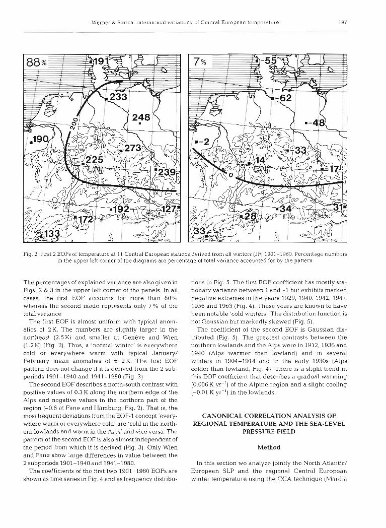
We derived EOFs of Central European temperature for the complete interval 1901-1980 (Fig. 2) as well as for the 2 subintervals 1901-1940 and 1941 -1980 (Fig. 3).

Werner & Storch: Interannual variability of Central European temperature 197

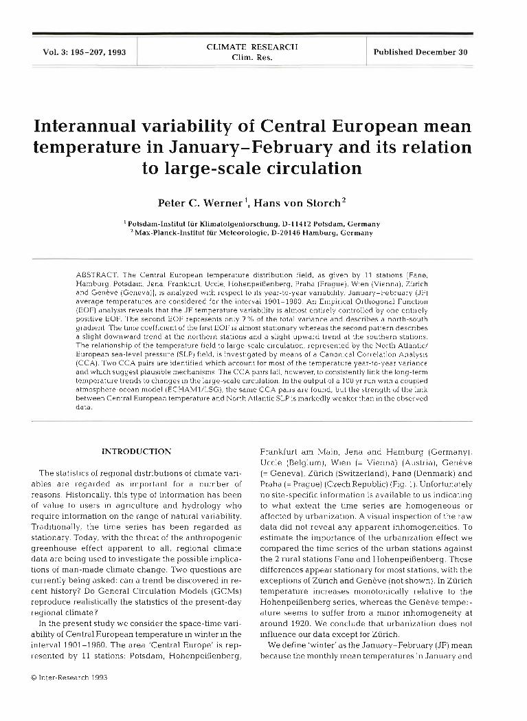
Fig. 2. First 2 EOFs of temperature at 11 Central European stations derived from all winters (JF) 1901-1980. Percentage numbers in the upper left corner of the diagrams are percentage of total variance accounted for by the pattern

The percentages of explained variance are also given in Figs. 2 & 3 in the upper left corner of the panels. In all cases, the first EOF accounts for more than 80% whereas the second mode represents only 7 % of the total variance.

The first EOF is almost uniform with typical anom- alies of 2K. The numbers are slightly larger in the northeast (2.5K) and smaller at Geneve and Wien (1.2K) (Fig. 2). Thus, a 'normal winter' is everywhere cold or everywhere warm with typical January/ February mean anomalies of +_ 2 K . The first EOF pattern does not change if it is derived from the 2 sub- periods 1901-1940 and 1941-1980 (Fig. 3)

The second EOF describes a north-south contrast with positive values of 0.3 K along the northern edge of the Alps and negative values in the northern part of the region (-0.6 at Fan0 and Hamburg; Fig. 2). That is, the most frequent deviations from the EOF-1 concept 'every- where warm or everywhere cold' are 'cold in the north- ern lowlands and warm in the Alps' and vice versa. The pattern of the second EOF is also almost independent of the period from which it is derived (Fig. 3). Only Wien and Fan0 show large differences in value between the 2 subperiods 1901-1940 and 1941-1980.

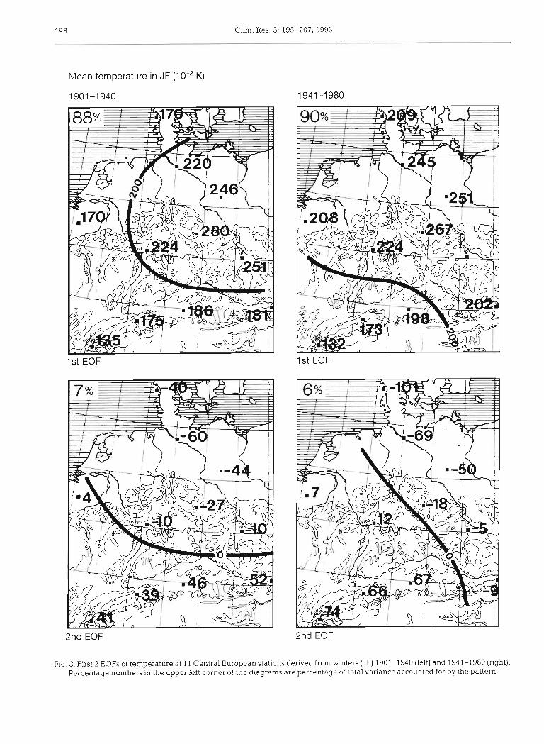
The coefficients of the first two 1901-1980 EOFs are shown as time series in Fig. 4 and as frequency distribu-

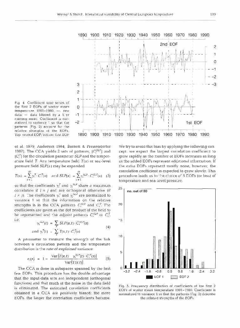
tions in Fig. 5. The first EOF coefficient has mostly sta- tionary variance between 1 and -1 but exhibits marked negative extremes in the years 1929, 1940, 1942, 1947, 1956 and 1963 (Fig. 4). These years are known to have been notable 'cold winters'. The distribution function is not Gaussian but markedly skewed (Fig. 5).

The coefficient of the second EOF is Gaussian dis- tributed (Fig. 5). The greatest contrasts between the northern lowlands and the Alps were in 1912,1936 and 1940 (Alps warmer than lowland) and in several winters in 1904-1914 and in the early 1930s (Alps colder than lowland; Fig. 4). There is a slight trend in this EOF coefficient that describes a gradual warming (0.006 K yr-') of the Alpine region and a slight cooling (-0.01 K yr-l) in the lowlands.

CANONICAL CORRELATION ANALYSIS OF REGIONAL TEMPERATURE AND THE SEA-LEVEL

PRESSURE FIELD

Method

In this section we analyze jointly the North Atlantic/ European SLP and the regional Central European winter temperature using the CCA technique (Mardia

Werner & Storch: Interannual variability of Central European temperature

Fig. 4 Coefficient time series of the first 2 EOFs of wlnter mean temperature 1901-1980. -: raw data; ---: data filtered by a 5 yr running mean. Coefficient is nor- malized to variance 1 so that the patterns (Fig. 2) account for the relative strengths of the EOFs. Top: second EOF; bottom: first EOF

et al. 1979, Anderson 1984, Barnett & Preisendorfer 1987). The CCA yields 2 sets of patterns, (CiSLP) and {C:) for the circulation parameter SLP and the temper- ature field T. Any temperature field T(x) or sea-level pressure field SLP(x) may be expanded

m m

T(x) = X y:. C ~ ( X ) and SLP(x) = &,SLP. C,SLP(x) (3) 1:l 1 = 1

so that the coefficients y: and y P P share a maximum correlation if i = j and are orthogonal otherwise (if i # j). The coefficients y: and y P P are normalized to variance 1 so that the information on the relative strengths is in the CCA patterns C,SLP and C,? The coefficients are given as the dot product of the field to be represented and the adjoint patterns or C:

and y:(t) = T(x, t ) . c ~ ( x ) X

A parameter to measure the strength of the link between a circulation pattern and the temperature distribution is the rate of explained variance:

The CCA is done in subspaces spanned by the first few EOFs. This procedure has the double advantage that the input-data sets are independent (orthogonal

We try to avoid this bias by applying the following con- cept: we expect the largest correlation coefficient to grow rapidly as the number of EOFs increases as long as the added EOFs represent add~tional information. If the extra EOFs represent mostly noise, however, the correlation coefficient is expected to grow slowly. This procedure leads us to the choice of 5 EOFs (or less) of temperature and sea-level pressure.

25 no. out of 80

-3.2 -2.4 -1.6 -0.8 0.0 0.8 1.6 2.4 3.2

EOF 1 m EOF2

functions) and that much of the noise in the data field Fig. 5. Frequency distribution of coefficients of the first 2 is eliminated. The estimated correlation coefficients EOFs of winter mean temperature 1901-1980, Coefflclent is

obtained in a CCA are positively biased: the normalized to variance 1 so that the patterns (Fig. 2) describe EOFs, the larger the correlation coefficients become. the relative strengths of the EOFs

200 Clim. Res. 3: 195-207, 1993

Fig. 6. First CCA pair of SLP and seasonal mean temperature for J F derived from the 1901-1940 subset Correlation coefficient estimated from the complete interval 1901-1980 is 0.64. (A) SLP pattern; repre- sents 39% of the total variance of SLP in the interval 1901-1980. (B) Temperature pattern (upper value) and field of percent- age of explained local variance (lower

value) in the interval 1901-1980

The CCA was carried out with the sea-level pressure and temperature data from the 'estimation' interval 1901-1940; the explained variances &;(X) and the correlation coefficients are calculated from the com- plete interval 1901-1980 including the 'test' interval 1941-1980.

Results

The first CCA pair (Fig. 6) has a correlation [between Y:(t) and ylSLP(t)] of 70% in the estimation period 1901-1940. The SLP pattern describes an anomalous southwesterly flow into Central Europe. This south- westerly flow advects anomalously warm maritime air

so that the temperature pattern is positive everywhere with maximum values of almost 2 K along the Alps and minimum values of 0.7 K a t Fans. In Fig. 6b the rate E ,

of explained local variance, as derived from the test sample 1941-1980, is also given. This rate 1s greater than 40% everywhere except for Zurich (31%), Hamburg (37 %) and Fans (22 %). Apparently, the first CCA pair determines mostly the southern part of the analysis area.

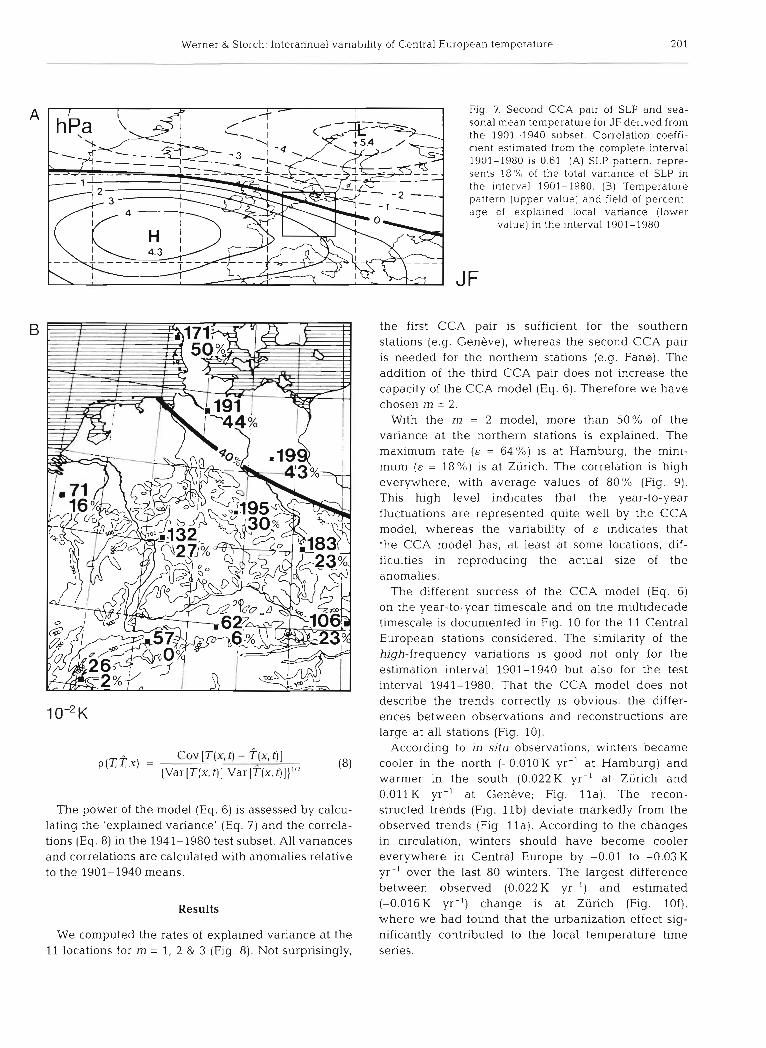
The second CCA pair (Fig. 7) specifies the northern part of the analysis area. The SLP field represents a strong northwesterly flow that affects mainly the northern part of Central Europe. There the typical temperature anomalies are almost 2 K (at Potsdam, Hamburg and Fans), and the rates of explained local variance are more than 40%. Along the Alps, at Geneve and Zurich, the typical anomalies are 0.6K with explained variances of less than 10 %.

CONSISTENCY OF TRENDS IN CIRCULATION AND TEMPERATURE

Method

We may use the results of the CCA analysis of the previous section to derive temperature anomalies indi- rectly using only anomalous circulation. This 'CCA model' is given by:

(von Storch et al. 1993) where m is the number of CCA pairs used.

The power of the model in Eq. (6) can be monitored either by the rate of the T-variance explained by T

Var [T(x, t) - ~ ( x , t)] E(? ;~ ,x ) = 1 -

Var [T(x, t ) ] (7)

or by the correIation between Tand f

Werner & Storch- Interannual variability of Central European temperature 201

p- P-

Fig. 7. Second CCA pair of SLP and sea- sonal mean temperature for J F derived from the 1901-1940 subset. Correlation coeffi- cient estimated from the complete interval 1901-1980 is 0.61 (A) SLP pattern. repre- sents 18% of the total vanance of SLP in the interval 1901 - 1980. (B) Temperature pattern (upper value) and field of percent- age of explained local variance (lower

value) in the interval 1901-1980

P ( T ~ ; x ) = Cov [T(x, t) - T ( X , t)]

(Var [T(x , t ) ] Var [?(X, t)])"' (8)

The power of the model (Eq. 6) is assessed by calcu- lating the 'explained variance' (Eq. 7) and the correla- tions (Eq. 8) in the 1941-1980 test subset. All variances and correlations a re calculated with anomalies relative to the 1901-1940 means.

Results

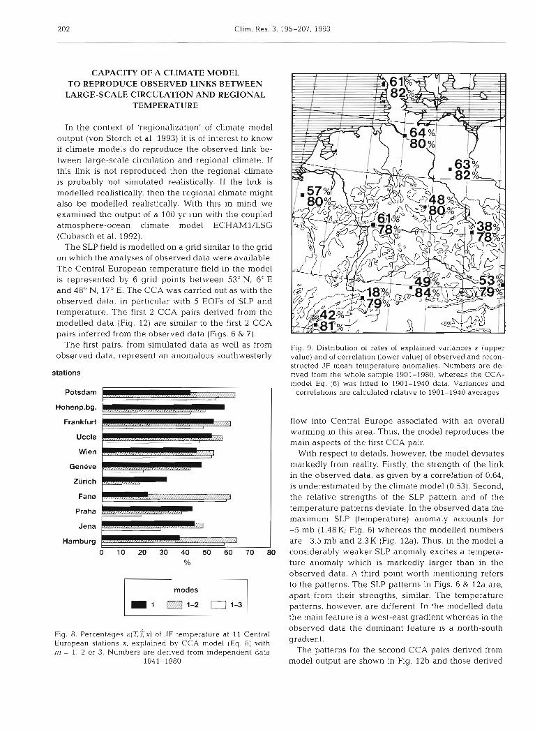
We computed the rates of explained variance a t the 11 locations for m = 1, 2 & 3 (Fig. 8). Not surprisingly,

the first CCA pair is sufficient for the southern stations (e.g. Geneve), whereas the second CCA pair is needed for the northern stations (e.g. Fans). The addition of the third CCA pair does not increase the capacity of the CCA model (Eq. 6). Therefore we have chosen m = 2.

With the m = 2 model, more than 50% of the variance at the northern stations is explained. The maximum rate ( E = 64%) is at Hamburg, the mini- mum (E = 18%) is at Zurich. The correlation is high everywhere, with average values of 80% (Fig. 9) . This high level indicates that the year-to-year fluctuations are represented quite well by the CCA model, whereas the variability of E indicates that the CCA model has, at least a t some locations, dif- ficulties in reproducing the actual size of the anomalies.

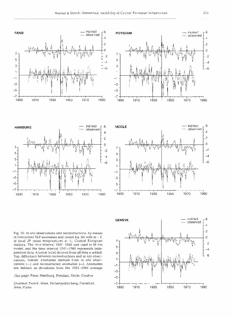
The different success of the CCA model (Eq. 6) on the year-to-year timescale and on the multidecade timescale is documented in Fig. 10 for the 11 Central European stations considered. The similarity of the high-frequency variations is good not only for the estimation interval 1901-1940 but also for the test interval 1941-1980. That the CCA model does not describe the trends correctly is obvious: the differ- ences between observations and reconstructions are large at all stations (Fig. 10).

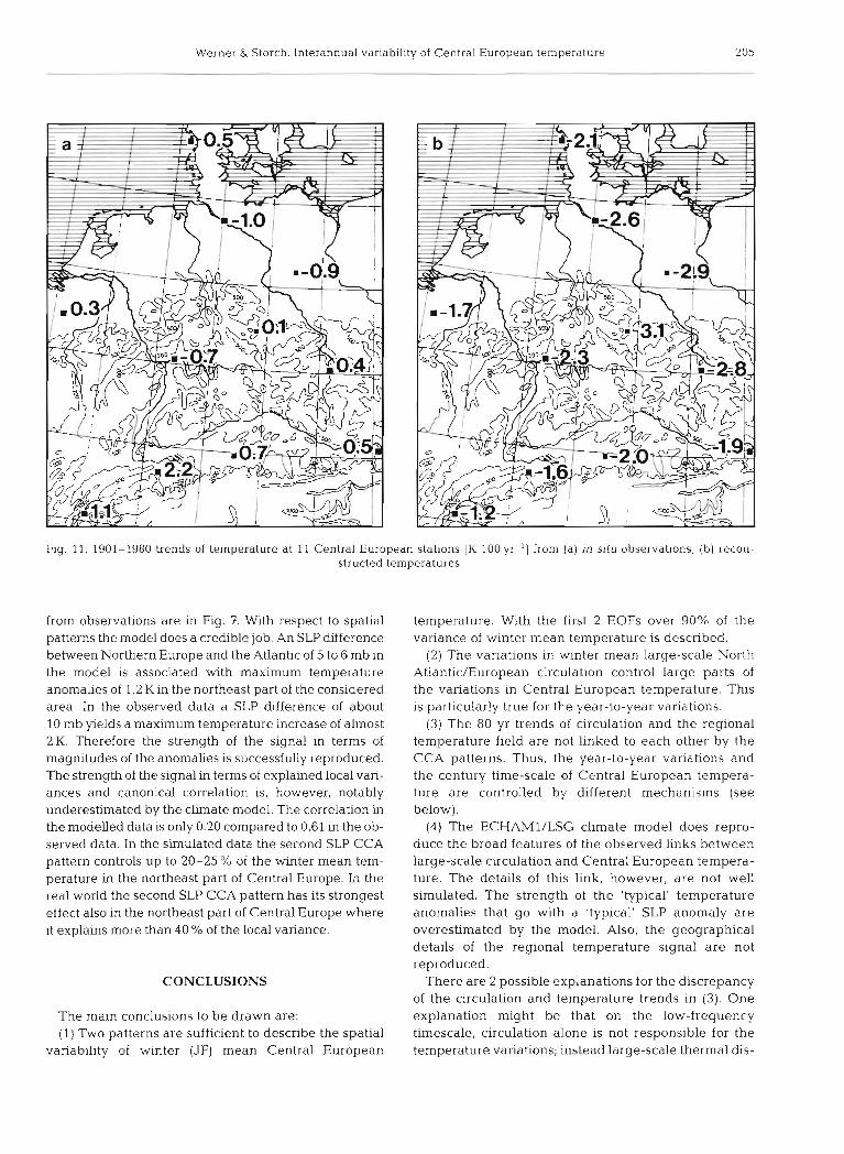
According to in situ observations, winters became cooler in the north (-0.010K yr-' a t Hamburg) and warmer in the south (0.022K yr-' at Zurich and 0.011K yr-' at Geneve; Fig. l l a ) . The recon- structed trends (Fig. l l b ) deviate markedly from the observed trends (Fig l l a ) . According to the changes in circulation, winters should have become cooler everywhere in Central Europe by -0.01 to -0.03 K yr-' over the last 80 winters. The largest difference between observed (0.022K yr-') and estimated (-0.016K yr-') change is a t Ziirich (Fig. l O f ) , where we had found that the urbanization effect sig- nificantly contributed to the local temperature time series.

202 Clim. Res. 3: 195-207, 1993

CAPACITY OF A CLIMATE MODEL TO REPRODUCE OBSERVED LINKS BETWEEN

LARGE-SCALE CIRCULATION AND REGIONAL TEMPERATURE

In the context of 'regionalization' of climate model output (von Storch et al. 1993) it is of interest to know if climate models do reproduce the observed link be- tween large-scale circulation and regional climate. If this link is not reproduced then the regional climate is probably not simulated realistically. If the link is modelled realistically, then the regional climate might also be modelled realistically. With this in mind we examined the output of a 100 yr run with the coupled atmosphere-ocean climate model ECHAMl/LSG (Cubasch et al. 1992).

The SLP field is modelled on a grid similar to the grid on which the analyses of observed data were available. The Central European temperature field in the model is represented by 6 grid points between 53" N, 6" E and 48' N, 17" E. The CCA was carried out as with the observed data, in particular with 5 EOFs of SLP and temperature. The first 2 CCA pairs derived from the modelled data (Fig. 12) are similar to the first 2 CCA pairs inferred from the observed data (Figs. 6 & 7 ) .

The first pairs, from simulated data as well as from observed data, represent an anomalous southwesterly

stations

Potsdam

Hohenp.bg.

Frankfurt - p- -

Uccle

Wien

Genhve

Ziirich

Praha

Jena

Hamburg

0 10 20 30 40 50 60 70 80

modes

Fig. 8. Percentages c ( ? ; t x ) of JF temperature at 11 Central European stations X, explained by CCA model (Eq. 6) with m = 1, 2 or 3. Numbers are derived from independent data

Fig. 9. Distribution of rates of expla~ned variances E (upper value) and of correlation (lower value) of observed and recon- structed JF mean temperature anomalies. Numbers are de- rived from the whole sample 1901-1980, whereas the CCA- model Eq. (6) was fitted to 1901-1940 data. Variances and

correlations are calculated relative to 1901-1940 averages

flow into Central Europe associated with an overall warming in this area. Thus, the model reproduces the main aspects of the first CCA pair.

With respect to details, however, the model deviates markedly from reality. Firstly, the strength of the link in the observed data, as given by a correlation of 0.64, is underestimated by the climate model (0.53). Second, the relative strengths of the SLP pattern and of the temperature patterns deviate. In the observed data the maximum SLP (temperature) anomaly accounts for -5 mb ( 1 . 4 8 K ; Fig. 6) whereas the modelled numbers are -3.5 mb and 2.3 K (Fig. 12a). Thus, in the model a considerably weaker SLP anomaly excites a tempera- ture anomaly which is markedly larger than in the observed data. A third point worth mentioning refers to the patterns. The SLP patterns in Figs. 6 & 12a are, apart from their strengths, similar. The temperature patterns, however, are different. In the modelled data the main feature is a west-east gradient whereas in the observed data the dominant feature is a north-south gradient.

The patterns for the second CCA pairs derived from 1941-1980 model output are shown in Fig. 12b and those derived

Werner & Storch: Interannual variability of Central European temperature

observed

HAMBURG UCCLE

7 7

5 5

3 3

1 1

-1 -1

-3 -3

-5 -5

-7 -7 I

1890 1910 1930 1950 1970 1990 1890 1910 1930 1950 1970 1990

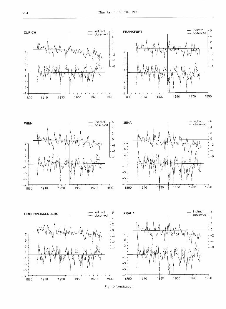
Fig. 10. In situ observations and reconstructions, by means of concurrent SLP anomalies and model Eq. (6) with m = 2, of local JF mean temperatures at 11 Central European stations. The time interval 1901-1940 was used to fit the model, and the time interval 1941-1980 represents inde- pendent data. A linear trend derived from all data is added. Top: difference between reconstructions and in situ obser- vations; bottom: anomalies derived from in situ obser- vations ( - - - ) and reconstructed anomalies (-). Anomalies are defined as deviations from the 1901-1940 average

This page: Fane, Hamburg, Potsdam, Uccle, Geneve

Overleaf: Ziirich, Wien. Hohenpelaenberg, Frankfurt, Jena, Praha

- indirect .---. observed

Werner & Storch: Interannual variability of Central European temperature

Fig. 11. 1901-1980 trends of temperature at 11 Central European stations [K 100 yr-'1 from (a) in situ observations, (b) recon- structed temperatures

from observations are in Fig. 7. With respect to spatial patterns the model does a credible job. An SLP difference between Northern Europe and the Atlantic of 5 to 6 mb in the model is associated with maximum temperature anomalies of 1.2 K in the northeast part of the considered area. In the observed data a SLP difference of about 10 mb ylelds a maximum temperature increase of almost 2 K . Therefore the strength of the signal in terms of magnitudes of the anomalies is successfully reproduced. The strength of the signal in terms of explained local vari- ances and canonical correlation is, however, notably underestimated by the climate model. The correlation in the modelled data is only 0.20 compared to 0.61 in the ob- served data. In the simulated data the second SLP CCA pattern controls up to 20-25 % of the winter mean tem- perature in the northeast part of Central Europe. In the real world the second SLP CCA pattern has its strongest effect also in the northeast part of Central Europe where it explains more than 40 % of the local variance.

CONCLUSIONS

The main conclusions to be drawn are: (1) Two patterns are sufficient to describe the spatial

variability of winter (JF) mean Central European

temperature. With the first 2 EOFs over 90% of the variance of winter mean temperature is described.

(2) The variations in winter mean large-scale North Atlantic/European circulation control large parts of the variations in Central European temperature. This is particularly true for the year-to-year variations.

(3) The 80 yr trends of circulation and the regional temperature field are not linked to each other by the CCA patterns. Thus, the year-to-year variations and the century time-scale of Central European tempera- ture are controlled by different mechanisms (see below).

(4) The ECHAMl/LSG climate model does repro- duce the broad features of the observed links between large-scale circulation and Central European tempera- ture. The details of this link, however, are not well simulated. The strength of the 'typical' temperature anomalies that go with a 'typical' SLP anomaly are overestimated by the model. Also, the geographical details of the regional temperature signal are not reproduced.

There are 2 possible explanations for the discrepancy of the circulation and temperature trends in (3). One explanation might be that on the low-frequency timescale, circulation alone is not responsible for the temperature variations; instead large-scale thermal dis-

206 Clim. Res. 3: 195-207, 1993

Fig. 12. First 2 pairs of CCA patterns inferred from the 100 yr output of a climate model (ECHAMULSG). Correlations are (a) 0.53 for the first pair and (b) 0.20 for the second pair Left diagrams show SLP patterns with the 6 model grid points representing Central Europe. The associated temperature distribution at these 6 grid points, together with the percentage of local temperature

variance, is shown in the right panels. Panels (a) should be compared with Fig. 6 and panels (b) with Fig. 7

tribution, and in particular North Atlantic SST, is relevant. An EOF analysis of Atlantic SST in January (Hense et al. 1990) revealed that the most important EOF descnbes a gradual warming of most of the Atlantic from the beginning of the century. Maximum trends are 0.016K yr-l from 1900 through 1960. This warming of the surface might counteract a cooling trend induced by the gradual weakening of the wintertime circulation in the North Atlantic/European region.

The other explanation would be that the data are inconsistent, i.e. that either the temperature trends or the circulation trends are incorrectly given by the data. The circulation trend has been documented by van Loon & Williams (1976) and has been shown to be consistent with trends in Iberian rainfall by von Storch et al. (1993). Are there reasons to suspect the temperature data? A wild-card in the present analysis is the urbanization effect: it is possible that the readings of temperature have systematically increased through the past 80 yr simply because of the increasing size and density of the towns in which many of the thermometers are placed.

ever, to the conclusion that this effect does not interfere with our results, apart from Zurich.

We propose as a more likely hypothesis that the vari- ability of the regional temperature on timescales of several decades is controlled not only by the circula- tion but also by low-frequency variations of Atlantic sea-surface temperature.

LITERATURE CITED

Anderson. C. W. (1984). An introduction to multivariate statistical analysis, 2nd edn. Wiley & Sons, New York

Barnett, T P., Preisendorfer, R. (1987). Origins and levels of monthly and seasonal forecast skills for United States surface air temperatures determined from canonical cor- relation analysis. Mon. Weather Rev. 115: 1825-1850

Cubasch, U., Hasselmann. K., Hock, H., Maier-Reimer. E., Mikolajewicz, U,, Santer, B. D., Sausen, R. (1992). Time- dependent greenhouse warming computations with a cou- pled ocean-atmosphere model. Clim. Dyn. 8: 55-69

Hess, P., Brezowsky, H. (1977). Katalog der GroDwetterlagen Europas, 3. verbesserte und erganzte Auflage. Ber. Dtsch.

The urbanization effect would imply an artificial posi- Wetterdienstes 113 Hense, A., Glowienka-Hense, R., von Storch, H., Stahler, U.

tive temperature trend. The comparison of the tempera- (1990). Northern Hemispheric atmospheric response to ture time series from urban stations with those from the chanaes of Atlantic Ocean SST on decadal time scales: a

d

2 rural stations Fan0 and HohenpeiDenberg led us, how- GCM experiment. Clim. Dyn. 4: 157-174

Werner & Storch: Interannual variability of Central European temperature 207

Mardia, K. V., Kent, J. T., Bibby, J. M. (1979). Multivariate analysis. Academic Press, London

Miller, A. J. , Teweles, S . , Woolf, H. M. (1967). Seasonal varia- tion of angular momentum transport at 500 mb. Mon. Weather Rev. 95: 427-439

Smirnov, I. P., Kazakova, L. L. (1966). Voprosy gidrodina- miteskol teoni klimata i dolgosrocnogo prognoza pogody. Trudy Mirovoj Meteorologitseskoj Centr 12: 43-63

Trenberth. K., Paolino, D. A. (1980). The northern hemisphere

Editor: G. Esser

sea-level pressure data set: trends, errors and discontinu- ities. Mon. Weather Rev. 108: 855-872

von Storch, H., Zonta, E. , Cubasch, U . (1993). Downscaling of global climate change estimates to regional scales: an application to Iberian rainfall in wintertime. J. Clim. 6: 1161-1171

van Loon, H.. Williams, J (1976). The connection between trends of mean temperature and circulation at the surface. I. Winter. Mon. Weather Rev. 104: 365-380

Manuscript first received: February 17, 1993 Revised version accepted: August 11, 1993