interception capacity of conventional depressed curb inlets and inlets with channel ... ·...
TRANSCRIPT

TECHNICAL REPORT 0-6842-1TxDOT PROJECT NUMBER 0-6842
Interception Capacity of Conventional Depressed Curb Inlets and Inlets with Channel Extension
Ben R. HodgesMichael E. BarrettMuhammad AshrafFrank E. Schalla
May 2018; Published September 2018
http://library.ctr.utexas.edu/ctr-publications/0-6842-1.pdf

Technical Report Documentation Page
1. Report No.
FHWA/TX-18/0-6842-1
2. Government
Accession No.
3. Recipient’s Catalog No.
4. Title and Subtitle
Interception Capacity of Conventional Depressed Curb Inlets and
Inlets with Channel Extension
5. Report Date
May 2018; Published September 2018
6. Performing Organization Code
7. Author(s)
Ben R. Hodges, Ph.D.; Michael E. Barrett, Ph.D.;
Muhammad Ashraf, and Frank E. Schalla
8. Performing Organization Report No.
0-6842-1
9. Performing Organization Name and Address
Center for Transportation Research
The University of Texas at Austin
3925 W. Braker Lane, 4th floor
Austin, TX 78759
10. Work Unit No. (TRAIS)
11. Contract or Grant No.
0-6842
12. Sponsoring Agency Name and Address
Texas Department of Transportation
Research and Technology Implementation Division
P.O. Box 5080
Austin, TX 78763-5080
13. Type of Report and Period Covered
Technical Report
January 2015–April 2018
14. Sponsoring Agency Code
15. Supplementary Notes
Project performed in cooperation with the Texas Department of Transportation.
16. Abstract
This report presents the results of a project investigating the performance of the TxDOT PCO curb inlet for effects of flush supports
and internal hydraulic controls. PCO inlets use flush supports for the top slab of inlets longer than 5 ft, which are thought to reduce
the interception capacity of curb inlets by as much as 50%. PCO inlets longer than 5 ft are divided into a main bay and side extension
chamber(s). Unlike a conventional inlet, flow in an extension does not fall directly into a large bay. Instead, an extension has a channel
directing the flow into the main bay, which has the potential to reduce the interception capacity.
Three topics were investigated: 1) The effect of structural slab supports on the performance of curb inlets, 2) the performance of
conventional depressed inlets under different flow conditions and road slopes, and 3) the effect of potential flow restrictions on the
interception capacity of curb inlets with channel extensions. An existing model of a roadway with adjustable slopes was modified to
accommodate a full-scale model of the depressed PCO inlet.
Experiments for on-grade 10 and 15 ft inlets showed no observable difference in the intercepted flow due to the presence of slab
supports. However, tests showed the present on-grade equations for long curb inlets significantly overestimate their capacity. A
correction factor was developed for computing the 100% interception flow and a new relationship for computing the inlet capture at
less than 100% interception condition. Tests showed the 10 ft PCO inlets on-grade are equivalent to a conventional inlet and requires
the same correction factor to compute capacity. The 15 ft PCO inlets should never be used on-grade due to clogging potential. Tests
for a submerged PCO extension in a sag show significant degradation such that 10 ft and 15 ft inlets will be 58% and 47% of expected
capacity. PCO inlets are not recommended to handle submerged sag conditions.
17. Key Words
Depressed curb inlets; Channel extensions; Flush slab
supports; Interception capacity
18. Distribution Statement
No restrictions. This document is available to the public
through the National Technical Information Service,
Springfield, Virginia 22161; www.ntis.gov.
19. Security Classif. (of report)
Unclassified
20. Security Classif. (of this page)
Unclassified
21. No. of pages
144
22. Price
Form DOT F 1700.7 (8-72) Reproduction of completed page authorized

Interception Capacity of Conventional Depressed Curb Inlets and
Inlets with Channel Extension
Ben R. Hodges
Michael E. Barrett
Muhammad Ashraf
Frank E. Schalla
CTR Technical Report: 0-6842-1
Report Date: May 2018; Published September 2018
Project: 0-6842
Project Title: Analysis of Curb Inlets in the new TxDOT Standard Inlet and Manhole Program
Sponsoring Agency: Texas Department of Transportation
Performing Agency: Center for Transportation Research at The University of Texas at Austin
Project performed in cooperation with the Texas Department of Transportation and the Federal Highway
Administration.

Center for Transportation Research
The University of Texas at Austin
3925 W. Braker Lane, Stop D9300
Austin, TX 78759
http://ctr.utexas.edu/

v
Disclaimers
Author’s Disclaimer: The contents of this report reflect the views of the authors, who are
responsible for the facts and the accuracy of the data presented herein. The contents do not
necessarily reflect the official view or policies of the Federal Highway Administration or the Texas
Department of Transportation (TxDOT). This report does not constitute a standard, specification,
or regulation.
Patent Disclaimer: There was no invention or discovery conceived or first actually reduced to
practice in the course of or under this contract, including any art, method, process, machine
manufacture, design or composition of matter, or any new useful improvement thereof, or any
variety of plant, which is or may be patentable under the patent laws of the United States of
America or any foreign country.
Engineering Disclaimer
NOT INTENDED FOR CONSTRUCTION, BIDDING, OR PERMIT PURPOSES.
Research Supervisor: Dr. Ben R. Hodges

vi
Acknowledgments
The authors would like to thank the technical and programmatic contributions provided by the
TxDOT staff, including Stan Hopfe, Saul Nuccitelli, and Wade Odell. The assistance of the staff
at the Center for Transportation Research has been greatly appreciated in preparation and
submission of deliverables. A special thanks to the CTR Library staff who have been instrumental
in helping us obtain reports and data sets of past experiments that were not readily available. We
also thank the staff of the Center for Water and the Environment, who help keep the administrative
wheels rolling.
vii
Table of Contents
Chapter 1: Introduction ............................................................................................................... 1
1.1 Background ........................................................................................................................... 1
1.2 Objectives .............................................................................................................................. 3
1.3 Approach ............................................................................................................................... 3
Chapter 2: Literature Review ...................................................................................................... 4
2.1 Street Hydraulics ................................................................................................................... 4
2.2 Design Approaches of Depressed Curb Inlets ....................................................................... 5
2.2.1 Curb Inlets Performance ................................................................................................. 5
2.2.2 HEC-22 Design Equations ............................................................................................. 6
2.2.3 Comparison of Curb Inlet Design Equations .................................................................. 8
2.3 Flush Slab Supports ............................................................................................................... 9
2.3.1 Potential Issues with Top Slab Supports ........................................................................ 9
2.3.2 Review for Impact of Slab Support in Previous Studies ................................................ 9
2.4 Inlets with Channel Extension ............................................................................................. 11
2.4.1 Overview ...................................................................................................................... 11
2.4.2 Inlets Installed On-Grade.............................................................................................. 12
2.4.3 Inlets Installed in a Sag ................................................................................................. 12
2.5 On Experiment Scaling ....................................................................................................... 13
2.6 Conclusions ......................................................................................................................... 15
Chapter 3: Experimental Step-up ............................................................................................. 16
3.1 Existing Modeling Facility .................................................................................................. 16
3.2 Constructed Elements .......................................................................................................... 18
3.2.1 Summary ....................................................................................................................... 18
3.2.2 Curb Inlet ...................................................................................................................... 21
3.2.3 V-Notch Weirs and Approach Channels ...................................................................... 23
3.2.4 Headbox ........................................................................................................................ 23
3.3 Flow Measurement .............................................................................................................. 25
3.3.1 Measurement Devices ................................................................................................... 25
3.3.2 Flow Equations ............................................................................................................. 26
3.3.3 Flow Measurement Device Calibration ........................................................................ 27
3.3.4 Uncertainty in Measurements ....................................................................................... 28
3.4 Repeatability Tests .............................................................................................................. 29
3.5 Determining and Modifying Model Roughness .................................................................. 30
viii
3.5.1 Experimental Procedure for Data Collection................................................................ 30
3.5.2 Data and Analysis ......................................................................................................... 31
3.5.3 Roughness Modification ............................................................................................... 32
3.6 Conclusions ......................................................................................................................... 32
Chapter 4: Effects of Slab Supports .......................................................................................... 33
4.1 Experimental Procedures for Data Collection ..................................................................... 33
4.2 Results and Analysis ........................................................................................................... 33
4.3 Conclusions ......................................................................................................................... 36
Chapter 5: Interception Capacity of Depressed Curb Inlets .................................................. 38
5.1 Introduction ......................................................................................................................... 38
5.2 Tests at Modified Roughness .............................................................................................. 38
5.3 Comparison between Experimental Results and HEC-22 Design Equations ..................... 40
5.4 Analysis of Assumptions in HEC-22 .................................................................................. 43
5.4.1 Overview ...................................................................................................................... 43
5.4.2 Linear Decrease in the Water Surface along Inlet’s Length ......................................... 43
5.4.3 Flow Conditions Immediately Upstream the Inlet ....................................................... 44
5.4.4 Evaluation of the Equivalent Slope (Se) ....................................................................... 46
5.5 Correction Factor for HEC-22 at 100% Interception Condition ......................................... 47
5.5.1 Overview ...................................................................................................................... 47
5.5.2 Data Collection and Regression Analysis .................................................................... 47
5.5.3 Deficiency of Curb Inlets on a Combination of Steep Grade and Flat Cross Slope ..... 50
5.6 Bypass Flow Conditions...................................................................................................... 53
5.7 Discussion of Izzard’s L2 Length Scale .............................................................................. 60
5.8 Conclusions ......................................................................................................................... 65
Chapter 6: Interception Capacity of Inlets with Channel Extension ..................................... 66
6.1 Introduction ......................................................................................................................... 66
6.2 Modifications to the Model ................................................................................................. 67
6.3 Inlet on Grade ...................................................................................................................... 69
6.3.1 Comparison between Conventional and PCO Inlets .................................................... 69
6.3.2 The Effect of Inlet Tail Water on Interception Capacity .............................................. 71
6.4 Inlet in a Sag ........................................................................................................................ 74
6.4.1 Testing the Extension of the PCO Inlet ........................................................................ 74
6.4.2 Comparison to HEC-22 Results ................................................................................... 77
6.5 Simplified Design Procedure for PCO Inlet On-Grade ....................................................... 79

ix
6.6 Expected Performance of the TxDOT PCU Inlet ................................................................ 80
6.7 Conclusions ......................................................................................................................... 81
Chapter 7: Conclusions .............................................................................................................. 82
7.1 Summary ............................................................................................................................. 82
7.2 Slab Supports....................................................................................................................... 82
7.3 Depressed Curb Inlets ......................................................................................................... 82
7.4 Inlets with Channel Extension ............................................................................................. 84
References .................................................................................................................................... 86
Appendix A: Summary of Recent Studies on Curb Inlets ...................................................... 89
Appendix B: Experimental Data ............................................................................................... 90

x
List of Figures
Figure 1: Front view of new TxDOT precast curb inlet outside roadway (PCO) extracted
from TxDOT file presd03.dgn (January 2015 revisions).......................................................... 2
Figure 2: Plan view of new TxDOT PCO extracted from file presd03.dgn (January 2015
revisions). .................................................................................................................................. 2
Figure 3: Upper inlet basin of TxDOT PCO 10-ft inlet. Manhole and concrete floor are of
separate component on which the upper inlet is stacked (photograph courtesy of
TxDOT)..................................................................................................................................... 2
Figure 4: Roadway sections: (a) uniform section, (b) composite section. ...................................... 4
Figure 5: Comparison of efficiency from prior experiments and HEC-22 computation for
a 15 ft curb inlet (from Table 1) at road geometry: Sx =2%, SL = 2%, n = 0.0166. ................. 8
Figure 6: Curb inlet (depressed) with flush slab support (Denver Urban Storm Drainage
Criteria Manual, V. 1, pg. ST-20). .......................................................................................... 10
Figure 7: Photograph from Appendix C in Hammonds and Holley (1995) with arrows
added. ...................................................................................................................................... 11
Figure 8: Illustration of the main bay and extension of a curb inlet (Oldcastle, 2018). ............... 12
Figure 9: Definitions of h and do based on an inclined inlet throat (modified after HEC-
22). .......................................................................................................................................... 13
Figure 10: Comparison between full-scale and 1:6 scaled models: a) undepressed inlet, b)
depressed inlet (modified after Zwamborn, 1966). ................................................................. 14
Figure 11: Upstream support cross section (Qian et al., 2013). .................................................... 17
Figure 12: Downstream support cross section (Qian et al., 2013). ............................................... 17
Figure 13: Physical model before modifications. ......................................................................... 18
Figure 14: Definition sketch of physical model with modifications. ............................................ 19
Figure 15: Completed full-scale model of conventional 15 foot curb inlet without internal
slab supports............................................................................................................................ 20
Figure 16: Upstream curb and gutter transition for the full-scale model of conventional
curb inlet. ................................................................................................................................ 20
Figure 17: V-notch weirs and approach channels designed for measurement of
interception in each bay of conventional 15 ft curb inlet. ....................................................... 21
Figure 18: Inlet pipe manifold with valves, and headbox. ............................................................ 21
Figure 19: Under construction – wood framework of 2x6 inch studs for conventional
depressed inlet. ........................................................................................................................ 22
Figure 20: Under construction – view from downstream of the 2x6 inch wood framework
for conventional 15 ft inlet. ..................................................................................................... 22
Figure 21: Graded sand variations test panel for matching existing roadway texture. ................. 24
Figure 22: Profile view of the designs for the three V-notch weirs. ............................................. 25
Figure 23: Manifold design. .......................................................................................................... 25
xi
Figure 24: Flow measurement calibration. Comparison of simultaneously measured flows
with the new V-notch weirs and the existing rectangular weir. .............................................. 27
Figure 25. Repeatability test. Ponded width profiles at 100% curb inlet interception, 15 ft
inlet length and SL =2%, SX =4%. .......................................................................................... 29
Figure 26: Manning’s roughness coefficient as a function of longitudinal slope (data from
Qian et al, 2013 for existing roadway). ................................................................................... 31
Figure 27: Intercepted flow rates for the 15 ft inlet with and without slab supports. ................... 34
Figure 28: Ponded widths for 15 ft inlet with and without slab supports (Test#24 and 59
in Appendix B). ....................................................................................................................... 35
Figure 29: Waves at an internal slab support for a 15 ft curb inlet (Test #60 in Appendix
B)............................................................................................................................................. 35
Figure 30: Waves around both internal slab supports for a 15 ft curb inlet (Test#60 in
Appendix B). ........................................................................................................................... 36
Figure 31: Intercepted flow rates for the 10 ft inlet with and without slab supports. ................... 36
Figure 32: Intercepted flow rates for the 10 ft inlet at the original and the modified
roughness for all tested slopes. ............................................................................................... 38
Figure 33: Ponded width upstream of the 10 ft inlet at the original and the modified
roughness for all tested slopes. ............................................................................................... 39
Figure 34: 100% interception flow rates for a 15 ft curb inlet. Experimental
measurements and HEC-22 computations for all tested slopes. ............................................. 40
Figure 35: 100% interception flow rates for a 15 ft curb inlet. Experimental
measurements and HEC-22 computations at different slope combinations. .......................... 40
Figure 36: 100% interception flow rates for a 10 ft curb inlet. Experimental
measurements and HEC-22 computations for all tested slopes. ............................................. 41
Figure 37: 100% interception flow rates for a 10 ft curb inlet. Experimental
measurements and HEC-22 computations at different slope combinations. .......................... 41
Figure 38: 100% interception flow rates for a 5 ft curb inlet. Experimental measurements
and HEC-22 computations for all tested slopes. ..................................................................... 42
Figure 39: 100% interception flow rates for a 5 ft curb inlet. Experimental measurements
and HEC-22 computations at different slope combinations. .................................................. 42
Figure 40: Assumed linear decrease in water surface profile along inlet length (modified
from the original paper of Izzard, 1950). ................................................................................ 43
Figure 41: Along-inlet water surface profile (measured from the depressed inlet’s
opening) at 100% interception for 15 ft inlet with (a) SL=2%; Sx=2%, (b) SL=2%;
Sx=4%. .................................................................................................................................... 44
Figure 42: Observed flow spread at the uniform gutter and the observed spread
immediately upstream the depressed inlet. ............................................................................. 45
Figure 43: Cross-section of observed water surface elevation immediately upstream a 10
ft depressed inlet at SL=4% and Sx=2%. ................................................................................. 45
Figure 44: Observed uniform gutter spread for Eo =1 experiments (spread at inlet equal to
depression width). ................................................................................................................... 46
xii
Figure 45: Eo computed with HEC-22 for experiments of Figure 44 compared to observed
Eo =1. ...................................................................................................................................... 46
Figure 46: Histogram of Eo values based on Se computed from experimental intercepted
flow rates. ................................................................................................................................ 47
Figure 47: Measured intercepted flow rates for 100% interception and computed by: a)
HEC-22, b) HEC-22 after correction factor applied. .............................................................. 49
Figure 48: Measured experimental inlet length for 100% capture (Wasley, 1960) and as
computed by HEC-22 at Sx =1.042%. .................................................................................... 51
Figure 49: 100% interception flow rate. Measured and computed with HEC-22 and HEC-
22 with CF correction for steep grade flows in all available data. ......................................... 52
Figure 50: 100% interception flow rate. Measured and computed with HEC-22 with the
CF’ Correction for comparison with Figure 49. ..................................................................... 52
Figure 51: Computed inlet efficiency (Equation 2.7) based on HEC-22 values for LT and
observed values LT, as compared to observed efficiency of Karaki and Haynie (1961). ....... 54
Figure 52: Intercepted flow vs. spread of gutter flow, 3.75 ft inlet at 0.4% SL and 2.1% SX
(data from Hammond and Holley, 1995). ............................................................................... 55
Figure 53: Non-dimensional spread vs. intercepted flow for data from Figure 52. ...................... 55
Figure 54: Linear relationship between T and Qi in different studies. ......................................... 56
Figure 55: Observed vs. computed m slopes from Equation 5.9 using data from six prior
studies. .................................................................................................................................... 57
Figure 56: Histogram of experimental inlet efficiency data. ........................................................ 58
Figure 57: Comparison between observed inlet efficiency from different studies and the
computed efficiency using: a) HEC-22, b) Equation 5.8. ....................................................... 58
Figure 58: Efficiency computed using m=2.25 and m from Equation 5.9 for six prior
studies. .................................................................................................................................... 59
Figure 59: Comparison between efficiencies computed using HEC-22 with and without
CF correction. ......................................................................................................................... 59
Figure 60: Disturbance line observed at the depressed zone in the physical model. .................... 61
Figure 61: Dimensionless diagram of curb inlet performance, modified after Bauer and
Woo (1964). ............................................................................................................................ 62
Figure 62: Modified dimensionless diagram for inlet performance, modified after Izzard
(1977). ..................................................................................................................................... 63
Figure 63: Relative prediction error () corresponding to L2/Li for tests at 100%
interception for Manning’s n= 0.016 and 0.012 using data from the present study. .............. 64
Figure 64: Relative Prediction error () corresponding to the ratio L2/Li for tests at 100%
interception from the current study and Karaki and Haynie (1961). ...................................... 64
Figure 65: Rear view of the modeled 15-ft inlet before modifications. ........................................ 66
Figure 66: Recirculation in the downstream extension of a 15 ft PCO inlet on-grade (plan
view). ...................................................................................................................................... 67
Figure 67: Upstream section of the model after modifications. .................................................... 67
xiii
Figure 68: Opening connecting the two 5-ft sections in the model. ............................................. 68
Figure 69: Front view of the10-ft PCO inlet and the locations of cross-sections A and B. ......... 68
Figure 70: PCO inlet and the modified model at cross-section A (in Figure 69). ........................ 69
Figure 71: PCO inlet and the modified model at cross-section B (in Figure 69). ........................ 69
Figure 72: Comparison between intercepted flow rates at the PCO and conventional inlet
model configurations. ............................................................................................................. 70
Figure 73: Excess inflow being diverted from the upstream extension to the main inlet
section. .................................................................................................................................... 71
Figure 74: Cross-section of the upstream extension for tail water at the upper lip of the
inlet. ........................................................................................................................................ 71
Figure 75: The two tested tail water levels, looking from inside the inlet. ................................... 72
Figure 76: Front view of the box used to control tail water (Level A setup). .............................. 72
Figure 77: Full box at level A steup.............................................................................................. 73
Figure 78: Comparison between intercepted flow rates at low and raised tail water
conditions. ............................................................................................................................... 73
Figure 79: Inflow into the upstream extension being diverted into the main bay (Level A
setup). ...................................................................................................................................... 74
Figure 80: The set-up for the fully-submerged inlet, looking downstream. ................................. 74
Figure 81: Fully-submerged inlet, looking upstream. ................................................................... 75
Figure 82: Intercepted flow rate at the extension of a PCO inlet as a function of the depth
upstream the inlet. ................................................................................................................... 76
Figure 83: Cross-section of the PCO extension. ........................................................................... 76
Figure 84: The observations and fitted equation for the intercepted flow rates at the PCO
extension as a function of water depth at the inlet. ................................................................. 77
Figure 85: Intercepted flow rates at the PCO extension as a function of water depth at the
inlet based on HEC-22 and Experimental results. .................................................................. 77
Figure 86: Intercepted flow rates at the 10-ft PCO inlet as a function of water depth at the
inlet based on HEC-22 and experimental results. ................................................................... 78
Figure 87: Intercepted flow rates at the 15-ft PCO inlet as a function of water depth at the
inlet based on HEC-22 and experimental results. ................................................................... 78
Figure 88: Percent ratio between the interception capacities based on model results and
HEC-22 vs. the water depth at the inlet. ................................................................................. 79
Figure 89: Observed and computed Qi using Equation 6.2. ......................................................... 80
xiv
List of Tables
Table 1: Regression coefficients and exponents from the literature for Equation (2.14). .............. 8
Table 2: Literature reviewed for evidence that flush slab supports cause a 50% reduction
in capture. .................................................................................................................................. 9
Table 3: Dimensions of the three identical approach channels. .................................................... 25
Table 4: Individual uncertainty quantities in Equation 3.8. .......................................................... 28
Table 5: Repeatability test. Flow rates for 100% interception with 15 ft inlet and SL =2%,
SX =4%. ................................................................................................................................... 30
Table 6: Tested road geometries and flow rates. .......................................................................... 30
Table 7: Average Manning’s n from this experiment and Qian et al. (2013). .............................. 31
Table 8: Measured values of Manning’s n after resurfacing the model. ...................................... 32
Table 9: Tested configurations for analysis of slab supports effects. ........................................... 33
Table 10: Summary of conducted tests and intercepted flow ranges at original roughness. ........ 34
Table 11: Change in inlet efficiency due to change in road roughness (data from Karaki
and Haynie, 1961). .................................................................................................................. 39
Table 12: Parameter ranges in the final dataset. ........................................................................... 48
Table 13: Iterative procedure to compute the 100% interception inlet length given the
gutter flow. .............................................................................................................................. 50
Table 14: Tested configurations for PCO inlet on-grade. ............................................................. 70
Table 15: Tested configurations of extension in a sag. ................................................................. 75
Table 16: Tested configurations in the data used in developing PCO inlet design
procedure. ................................................................................................................................ 80
Table 17: Summary of recommendations and conclusions. ......................................................... 83
Table A-1: Curb inlet studies from the recent literature ............................................................... 89
Table B-1: Physical model data recorded during experiments for 15 ft curb inlet without
slab supports............................................................................................................................ 91
Table B-2: Physical model data recorded during experiments for 15 ft curb inlet with slab
supports. .................................................................................................................................. 96
Table B-3: Physical model data recorded during experiments for 10 ft curb inlet without
slab supports.......................................................................................................................... 101
Table B-4: Physical model data recorded during experiments for 10 ft curb inlet with slab
supports. ................................................................................................................................ 109
Table B-5: Physical model data recorded during experiments for 5 ft curb inlet. ...................... 113
Table B-6: Physical model data recorded during experiments at the new roughness for 10
ft curb inlet without slab support. ......................................................................................... 119
Table B-7: Experimental results of 10 ft PCO inlet on-grade .................................................... 127
Table B-8: Experimental results of 4.5 ft PCO extension in a sag ............................................. 129

1
Chapter 1: Introduction
1.1 Background
Storm-water runoff on roadways is typically collected and conveyed to subsurface sewers using
storm drain inlets. Curb-opening inlets are one of the commonly used storm drain inlets, which
consist of vertical openings in the curb covered by a top slab. Curb inlets are commonly used rather
than grate inlets as they are less susceptible to clogging by debris, pose minor interference to traffic
operation, and are safe for pedestrians and cyclists (TxDOT, 2016). Curb inlets are sized and
placed along a road to maintain a safe spread of water from the curb to reduce the chances of
vehicle hydroplaning. Accuracy of curb inlet interception equations is a critical issue for safe
roadway design as over-prediction of the interception will lead to roads with greater flow
downstream of the inlet and a larger spread from the curb than desired. The accepted curb inlet
design standard is the third edition of the Urban Drainage Design Manual (Brown et al., 2009—
herein HEC-22), which contains the FHWA's guidelines and recommended design procedures.
HEC-22 equations are widely used in design of roadway drainage (Hammonds and Holley, 1995),
and are implemented in TxDOT (2016).
Commercial storm drainage software typically includes the HEC-22 equations, e.g., the
StormCAD V8 XM user manual states that HEC-22 1996 edition is used for inlet computations
and Innovyze InfoSWMM allows users to specifically select HEC-22 inlets as well as other
approaches. The US EPA-supported public-domain Storm Water Management Model (SWMM)
is often used as an engine for commercial software but does not directly implement the HEC-22
equations. Instead, the user must design an orifice to represent a storm drain (Rossman, 2017). In
general, limited documentation is readily available on proprietary software implementation and
much of the detail is only accessible through the application graphical user interface (GUI).
Analysis of methods used in commercial software was beyond the scope of this study.
The new TxDOT standard pre-cast on-grade curb inlet, Type PCO (Figure 1 and Figure 2), uses
6-inch flush supports for the top slab when extensions are used on the right, left, or both sides of
the main inlet. These slab supports are thought by HEC-22 to decrease the interception capacity of
inlets by as much as 50%. However, HEC-22 doesn’t provide any guidance regarding quantifying
these effects.
The standard hydraulic calculations for the design of on-grade curb inlets assume free-fall
overflow from the lip of the inlet into the sewer system, and submerged inlets in a sag configuration
are based on orifice flow controlled by the inlet opening. However, some designs of long curb
inlets divide the inlet into a main bay with side extension chambers. Unlike a conventional inlet,
flow intercepted through an extension does not fall directly into the main bay. Instead the extension
provides a horizontal channel directing the intercepted flow, as shown in Figure 3 for the TxDOT
PCO inlet. For a compact design the cross-section of the extension channel is typically smaller
than the cross-section of the curb inlet itself. This reduction in cross-section can cause the
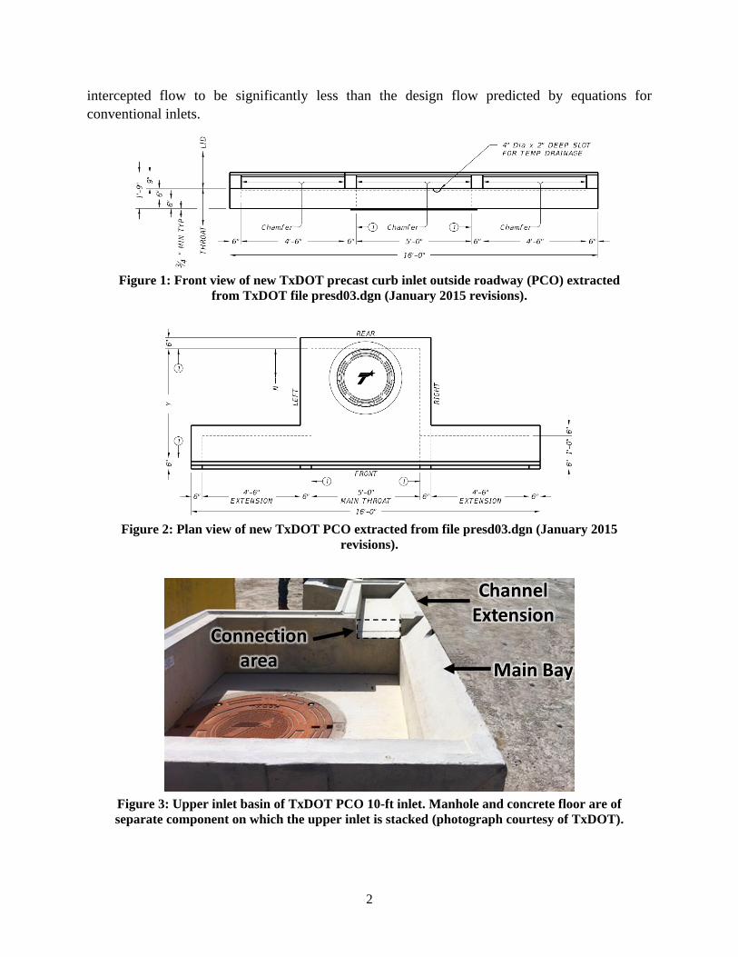
2
intercepted flow to be significantly less than the design flow predicted by equations for
conventional inlets.
Figure 1: Front view of new TxDOT precast curb inlet outside roadway (PCO) extracted
from TxDOT file presd03.dgn (January 2015 revisions).
Figure 2: Plan view of new TxDOT PCO extracted from file presd03.dgn (January 2015
revisions).
Figure 3: Upper inlet basin of TxDOT PCO 10-ft inlet. Manhole and concrete floor are of
separate component on which the upper inlet is stacked (photograph courtesy of TxDOT).

3
1.2 Objectives
The main objective of this project is to provide updated design guidance on the performance of the
TxDOT PCO inlet. This objective involves the investigation of three issues:
1) The effect of structural slab supports on the performance of curb inlets.
2) The performance of standard inlets under various flow conditions and road slopes.
3) The effect of potential flow restrictions on the interception capacity of inlets with channel extensions.
1.3 Approach
A pure analytical approach to this problem seemed implausible due to the complexity of flow in
the vicinity of curb inlets. Although computational models are possible, these require verification
against experiments before confidence in their results can be gained and such experiments (prior
to the present work) did not exist. Therefore, the approach of this study was to conduct full-scale
experiments for various roadway slope configurations and flow conditions. Modifications were
made to an existing physical model of a roadway at the University of Texas to accommodate a
full-scale model of a depressed curb inlet. Conventional inlets of 5, 10, and 15 ft were tested with
and without slab supports. The 10-ft PCO inlet was tested on-grade and an extension was tested in
a sag. The literature was surveyed for experimental data for depressed inlets to be used with results
from this study in assessing and updating the current design guidelines.
4
Chapter 2: Literature Review
2.1 Street Hydraulics
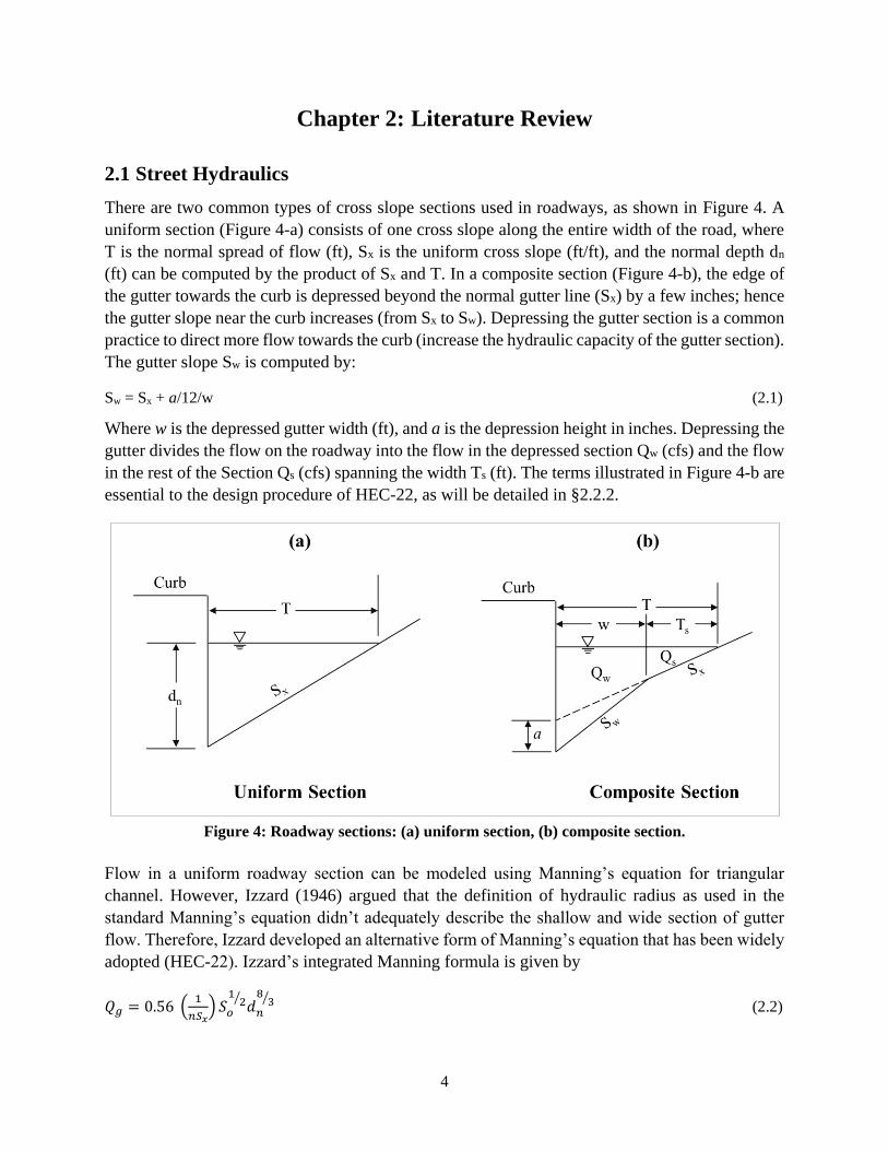
There are two common types of cross slope sections used in roadways, as shown in Figure 4. A
uniform section (Figure 4-a) consists of one cross slope along the entire width of the road, where
T is the normal spread of flow (ft), Sx is the uniform cross slope (ft/ft), and the normal depth dn
(ft) can be computed by the product of Sx and T. In a composite section (Figure 4-b), the edge of
the gutter towards the curb is depressed beyond the normal gutter line (Sx) by a few inches; hence
the gutter slope near the curb increases (from Sx to Sw). Depressing the gutter section is a common
practice to direct more flow towards the curb (increase the hydraulic capacity of the gutter section).
The gutter slope Sw is computed by:
Sw = Sx + a/12/w (2.1)
Where w is the depressed gutter width (ft), and a is the depression height in inches. Depressing the
gutter divides the flow on the roadway into the flow in the depressed section Qw (cfs) and the flow
in the rest of the Section Qs (cfs) spanning the width Ts (ft). The terms illustrated in Figure 4-b are
essential to the design procedure of HEC-22, as will be detailed in §2.2.2.
Figure 4: Roadway sections: (a) uniform section, (b) composite section.
Flow in a uniform roadway section can be modeled using Manning’s equation for triangular
channel. However, Izzard (1946) argued that the definition of hydraulic radius as used in the
standard Manning’s equation didn’t adequately describe the shallow and wide section of gutter
flow. Therefore, Izzard developed an alternative form of Manning’s equation that has been widely
adopted (HEC-22). Izzard’s integrated Manning formula is given by
𝑄𝑔 = 0.56 (1
𝑛𝑆𝑥) 𝑆𝑜
12⁄
𝑑𝑛
83⁄ (2.2)

5
Where Qg is the total gutter flow (cfs), n is Manning’s roughness coefficient, and So is the
longitudinal slope of the roadway (ft/ft). Equation 2.2 yield 18% higher roughness coefficient
value compared to the standard Manning equation for a triangular channel (Izzard, 1946).
2.2 Design Approaches of Depressed Curb Inlets
2.2.1 Curb Inlets Performance
Inlet interception can be increased by increasing the inlet length, roadway cross slope, and/or
roadway roughness, all of which help direct flow into the inlet. Conversely, the inlet interception
is decreased by increasing the roadway longitudinal slope (Jens, 1979), which tends to make water
flow past the inlet. Experiments have also shown that depressing the gutter section at an inlet also
increases interception (Johns Hopkins University, 1956). Another method of increasing the design
inlet interception is by allowing a small portion of the flow in the gutter to bypass the inlet. Because
of nonlinearity in the inlet equations, allowing a small bypass flow (< 5%) typically increases the
inlet interception greater than the bypassed amount, thus leading to a more cost-effective
configuration for a series of inlets (Karaki and Haynie, 1961).
The majority of curb inlets equations in the literature are based on empirical data fit to experiments.
Experiments were conducted for specific depression geometry and inlet length(s), and for one or
more roadway slope combinations. Regression analysis is then carried out to relate the intercepted
flow into the inlet to the normal depth (dn) or spread (T). Examples of these studies are McEnroe
et al. (1999), Kranc et al. (2001), and Fiuzat et al. (2000). Equations based solely on fits to
empirical data should be applied only to inlets matching the tested configuration for road slope,
inlet length, and the range of flow conditions. Other equations are based on theory with empirically
calibrated coefficients. For example, Izzard (1950) assumed that the flow across the inlet lip is
critical (i.e., the inlet is behaving like a weir) and that the water depth decreases linearly along the
inlet length. The discharge dQ per length dL of the inlet was integrated for the entire inlet length
to get the total flow into the inlet (Qi). The coefficients of the resulting equation were then
calibrated using experimental data from the University of Illinois. Equations based on theory with
well-behaved empirical coefficients can be applied to a wider range of cases, but care still must be
taken when extrapolating beyond the tested conditions. Other examples of these studies are
Hammond and Holley (1995), and Uyumaz (2002).
Design equations and charts are more accessible to practitioners compared to (commercial)
numerical models, which contributes to the scarcity of the use of numerical models in the literature.
Examples of the few computational studies are Jiang (2007) and Fang et al. (2010), which use the
numerical model FLOW-3D in evaluating curb inlet performance. Table A-1 (Appendix A)
provides a summary of curb inlet studies over the past 25 years that are available in the literature.
These studies typically caution that their equations cannot be used beyond their specific tests, and
clearly a relatively small range of inlet lengths have been examined.

6
2.2.2 HEC-22 Design Equations
The HEC-22 design manual can be considered the accepted (albeit imperfect) state of the art in
curb inlet design and is implemented within TxDOT (2016). The basic approach of HEC-22 is
used throughout the USA, although alternative approaches (particularly for grate inlets) have been
proposed (Gomez and Russo, 2005, 2011; Comport and Thorton, 2012).
The HEC-22 design procedures are based on computing an inlet efficiency (E), defined from the
intercepted flow rate (Qi) by the inlet and the total gutter flow rate upstream of the inlet (Qg) in a
ratio:
E =Q i
Qg
(2.3)
The bypass flow (Qb) that continues in the gutter downstream of the inlet is obtained by mass
conservation as:
Q
b= Q
g- Q
i (2.4)
HEC-22 uses an empirical equation for the required length of a non-depressed curb opening inlets
for 100% interception (i.e., E = 1), defined as:
LT
= KuQ
g
0.42SL
0.3 1
nSx
æ
èç
ö
ø÷
0.6
(2.5)
where Ku = 0.817 (SI) or 0.6 (English). This equation is based on the work of Izzard (1950):
LT= K Qg0.44 SL
0.28 ( 1
nSx )
0.56
(2.6)
where K=1.51 (SI) or 1.03 (English). HEC-22 approximates the exponents in Equation 2.6, but
there is a noticeable difference between the coefficients K and Ku. Izzard obtained Equation 2,6
with K = Ku= 0.6 based on the theoretical assumptions discussed in § 2.2.1. However, Izzard
modified the value of K to match a set of experimental data. Hammond and Holley (1995) showed
that using Ku instead K in Equation 2.6 provided better match with their experimental results.
Based on this discussion, we can safely conclude that HEC-22 uses the same theoretical
assumptions first proposed by Izzard (1950). Where the installed curb inlet length (Lc) is less than
LT for the design Qg, HEC-22 recommends an efficiency equation for use with Equation 2.3 of the
form:
E = 1- 1-L
c
LT
æ
èç
ö
ø÷
1.8
(2.7)
It follows that the bypass flow is obtained by manipulating Equations 2.3–2.6 to obtain:
7
Qb
= Qg
1-L
c
LT
æ
èç
ö
ø÷
1.8
(2.8)
HEC-22 extends the non-depressed inlet equations (above) for use with depressed curb inlets by
defining an equivalent cross slope, Se, to replace Sx in Equation 2.5:
S
e= S
x+S
w
' Eo (2.9)
where Sw'
is the cross slope of the depressed gutter section measured from the cross slope of the
pavement, and Eo is the ratio of flow in the depressed section to the total gutter flow. The depressed
gutter section cross slope measured from the pavement cross slope, Sw'
, is defined as:
Sw' = 𝑎/12/w (2.10)
where a is in inches and w is in ft. Sw is computed by Equation 2.1.
HEC-22 provides the following expression to compute Eo:
(2.11)
For a depressed curb inlet Equation 2.5 becomes:
LT
= KuQ
g
0.42SL
0.3 1
nSe
æ
èç
ö
ø÷
0.6
(2.12)
i.e., the same form and exponents as Equation 2.5 are retained, but Se is substituted for Sx. It should
be noted that Equation 2.11 applies for an inlet with a continuously depressed gutter. For an inlet
with a locally depressed gutter, the uniform gutter section upstream the inlet transitions gradually
into a fully depressed section at the inlet. According to HEC-22, the local depression does not
direct the flow into the inlet and the portion of the flow in the depressed section is determined from
the uniform gutter section upstream the transition region. For a uniform section, Sx = Sw; therefore
Equation 2.11 for Eo reduces to:
Eo = 1 – [1 – (w/T)]2.67 (2.13)
Although capturing the entire design gutter flow (i.e., Lc = LT, E=1, Qb=0) might seem preferable,
the power relationship in Equation 2.7 implies that reductions of installed curb length (Lc < LT)
are not linearly related to the efficiency. It follows that a relatively small bypass can allow a
significantly shorter inlet. Using the HEC-22 approach with Equation 2.7, an inlet length that is
81% of LT (19% reduction in length) leads to 5% bypass (95% capture), which is conservative
compared to studies of Fiuzat (2000) and Izzard (1977), who noted inlet lengths that were 75% of
8
LT had only 5% bypass. This concept is implemented within TxDOT (2016), where a bypass flow
up to 0.5 cfs is allowed where capturing the entire design gutter flow is not necessary.
2.2.3 Comparison of Curb Inlet Design Equations
For the Colorado Type R depressed curb inlet, Comport and Thorton (2012) and Guo and
MacKenzie (2012) developed revised sets of coefficients and exponents for the LT computation of
Equation 2.12 from HEC-22, which can be written in a general depressed curb inlet form as
LT=NQ
g
a SL
b 1
nSe
æ
èç
ö
ø÷
c
(2.14)
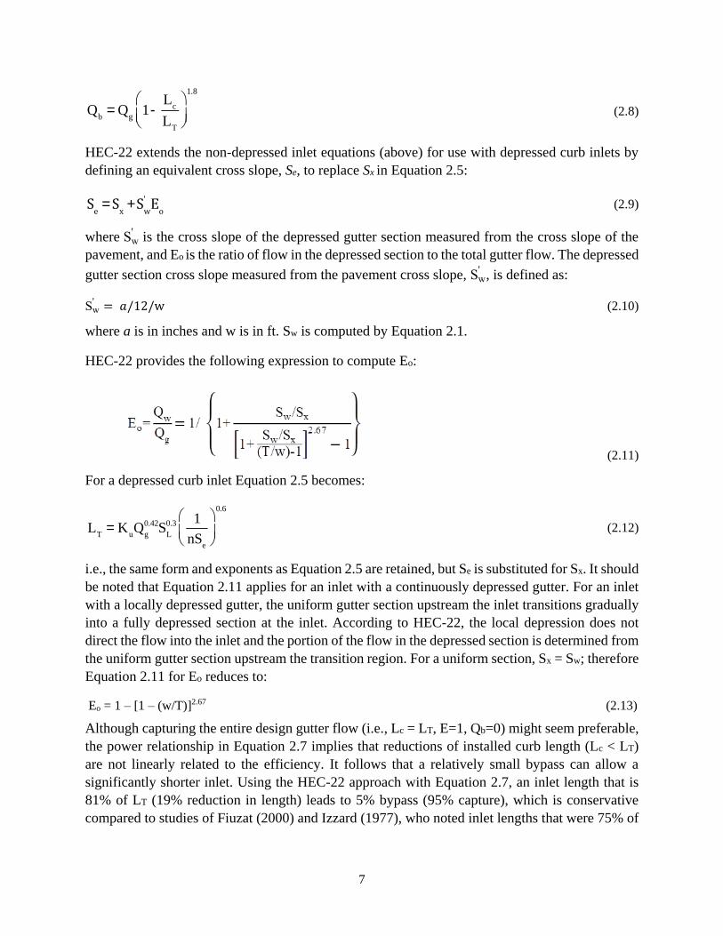
The different recommendations are shown in Table 1 and graphed in Figure 5. Although these
results show a significant departure from HEC-22, the accuracy of Comport and Thornton (2012)
has been questioned by Russo and Gomez (2014), whose experiments supported HEC-22, albeit
for grate inlets (Gomez and Russo, 2005 & 2011).
Table 1: Regression coefficients and exponents from the literature for Equation (2.14).
N [SI (English)] a b c
HEC-22 / TxDOT (2016) 0.817 (0.6) 0.42 0.3 0.6
Comport and Thornton (2012) 0.493 (0.176) 0.62 -0.021 0.49
Guo and Mackenzie (2012) (0.38) 0.51 0.06 0.46
Figure 5: Comparison of efficiency from prior experiments and HEC-22 computation for a
15 ft curb inlet (from Table 1) at road geometry: Sx =2%, SL = 2%, n = 0.0166.
Furthermore, the presence of a negative exponent for b in the Comport and Thorton (2012) implies
a departure from the physics of the theoretical model used to develop LT, indicating that their
approach is an empirical fit that might not be applicable beyond their tested system.

9
2.3 Flush Slab Supports
2.3.1 Potential Issues with Top Slab Supports
The new TxDOT standard pre-cast on-grade curb inlet, Type PCO (Figure 1 and Figure 2), uses
6-inch flush supports for the top slab for inlets longer than 5 ft (with one or more extensions
installed next to the main bay). Although flush slab supports are not uncommon in practice, HEC-
22 notes that:
“Top slab supports placed flush with the curb line can substantially reduce the interception
capacity of curb openings. Tests have shown that such supports reduce the effectiveness of
openings downstream of the support by as much as 50%.”
HEC-22 recommends that supports should be “recessed several inches from the curb line and
rounded.” However, HEC-22 does not provide any citation for studies supporting these
recommendations. Furthermore, no information is provided on quantifying the effects of flush slab
supports. Thus, the effect of such supports on performance of the new TxDOT Type PCO curb
inlet is unknown.
Storm water drainage computational software (e.g., StormCAD) typically use the HEC-22
equations, but we have been unable to find any vendor documentation related to any reduction
factor applied for slab supports. This null result is not definitive as these software applications do
not have comprehensive manuals detailing every feature
available through their graphical user interface (GUI). A
detailed review of storm drainage software GUIs was
beyond the scope of the present project.
2.3.2 Review for Impact of Slab Support in Previous
Studies
Curb inlet efficiency for roadway drainage has been
studied for more than 60 years, as summarized in reviews
of Holley et al. (1992), Hammonds and Holley (1995),
Thompson et al. (2003), and Jiang (2007). None of these
reviews mention investigations of the effects with and
without slab supports, although some research clearly
used models that included slab supports (e.g., Hammonds
and Holley, 1995; Comport and Thornton, 2012). Further
review of the literature (Table 2) has not provided any
evidence for the contention of HEC-22 that flush slab
supports have a 50% reduction in capture effectiveness.
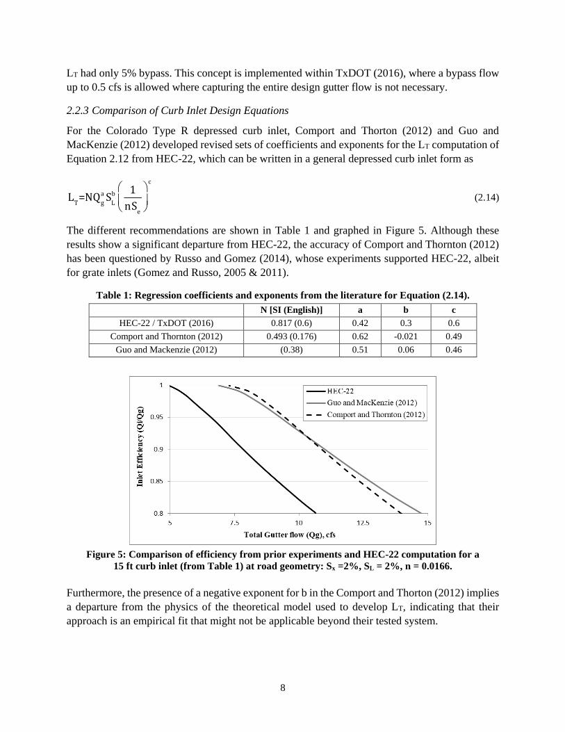
It is clear that flush structural slab supports are used in
practice despite the HEC-22 admonition, e.g., Figure 6
from the Denver Urban Storm Drainage Criteria
Table 2: Literature
reviewed for evidence that
flush slab supports cause a
50% reduction in capture.
Izzard (1950)
Johns Hopkins University (1956)
Zawmborn (1966)
Izzard (1977)
Bowman (1988)
Hotchkiss and Bohac (1991)
Soares (1991)
Holley et al. (1992)
Uyumaz (1992, 1994, 2002)
Hotchkiss (1994)
Hammond and Holley (1995)
MacCallan and Hotchkiss (1996)
McEnroe and Wade (1998)
McEnroe et al. (1999)
Fiuzat et al. (2000)
Spaliviero et al. (2000)
Kranc et al. (1998, 2001)
Guo (2006)
Jiang (2007)
Fang et al. (2010)
Comport and Thorton (2012)
Guo and MacKenzie (2012)
10
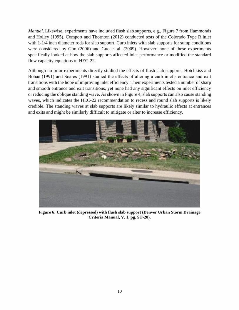
Manual. Likewise, experiments have included flush slab supports, e.g., Figure 7 from Hammonds
and Holley (1995). Comport and Thornton (2012) conducted tests of the Colorado Type R inlet
with 1-1/4 inch diameter rods for slab support. Curb inlets with slab supports for sump conditions
were considered by Guo (2006) and Guo et al. (2009). However, none of these experiments
specifically looked at how the slab supports affected inlet performance or modified the standard
flow capacity equations of HEC-22.
Although no prior experiments directly studied the effects of flush slab supports, Hotchkiss and
Bohac (1991) and Soares (1991) studied the effects of altering a curb inlet’s entrance and exit
transitions with the hope of improving inlet efficiency. Their experiments tested a number of sharp
and smooth entrance and exit transitions, yet none had any significant effects on inlet efficiency
or reducing the oblique standing wave. As shown in Figure 4, slab supports can also cause standing
waves, which indicates the HEC-22 recommendation to recess and round slab supports is likely
credible. The standing waves at slab supports are likely similar to hydraulic effects at entrances
and exits and might be similarly difficult to mitigate or alter to increase efficiency.
Figure 6: Curb inlet (depressed) with flush slab support (Denver Urban Storm Drainage
Criteria Manual, V. 1, pg. ST-20).
11
Figure 7: Photograph from Appendix C in Hammonds and Holley (1995) with arrows
added.
Although the figure was poorly reproduced in the PDF digitization, it is still possible to
observe the build-up of waves associated with the two supports (arrows).
Arguably, numerical simulations could provide a means of analyzing curb inlet configurations for
various types of slab supports (or no supports at all). Fang et al. (2010) used numerical simulations
(FLOW-3D) of the TxDOT Type C and D inlets previously studied in the laboratory by Hammonds
and Holley (1995). Unfortunately neither Fang et al. (2010) nor the dissertation of Jiang (2007)
provide confidence that FLOW-3D is correctly representing the complex flows around slab
supports. In particular, the numerical model was calibrated from Subramanya and Awasthy (1972)
experimental data, which was generated in a study of side-weir flow without any internal supports.
Thus, the ability of the FLOW-3D model (or any other model) to predict the effects of supports-
either recessed or flush with the curb- is as yet unproven.
2.4 Inlets with Channel Extension
2.4.1 Overview
Conventional curb inlets consist of an opening in the curb that leads to an underground basin that
spans the entire inlet length. Some designs of curb inlets restrict the length of the basin to only a
portion of the total inlet length (i.e., main bay), and the rest of the inlet length is added as a channel
attached on one or both sides of the main bay as shown in Figure 8. Saving on excavation, concrete,
and installation costs is the main motivation behind this inlet design. Curb inlets with channel
extensions are commonly used around the US, e.g. South Carolina inlet Type-5, 7, 17, 18; TxDOT
Type-C; Arkansas rectangular drop inlet; Oregon attachment to CG-1 and CG-2 inlets.

12
Figure 8: Illustration of the main bay and extension of a curb inlet (Oldcastle, 2018).
TxDOT PCO inlets (longer than 5 ft) consist of a 5 ft main bay and one or two 4.5 ft extension
chambers. The cross-section of the extension is 5” high and 12” wide, which is 20% of the area of
the opening of the inlet (as shown previously in Figure 3 with the connection area highlighted).
Accordingly, Flow intercepted by the 4.5 ft extension is expected to pass through a much smaller
section compared to the opening of the extension. As a convenience in nomenclature, we will call
these 5 ft extensions.
2.4.2 Inlets Installed On-Grade
A concern of TxDOT is that the design of the extensions of the standard PCO inlet might have the
potential to induce flow restrictions affecting the interception capacity. There are two fundamental
concerns: 1) the flow restriction at the connection of the upstream extension to the main chamber
for an on-grade configuration with a low tail-water could limit the inflow into the main chamber
and thus degrade the interception capacity, and 2) a high tail-water condition that submerged the
connection between the extension and the main chamber could cause further degradation in
capacity.
2.4.3 Inlets Installed in a Sag
When the flow depth in the gutter exceeds the height of the inlet opening, a conventional curb-
inlet in a sag is expected to operate as an orifice with the inlet-opening acting as the opening area
of the orifice. However, the design of the extensions of the PCO inlet might alter the expected
inlet-operation and reduce the interception capacity. This concern is due the relatively small area
of the opening connecting the extension to the main bay as compared to the inlet-opening.
HEC-22 proposes an orifice-flow equation for the interception capacity of a submerged inlet in a
sag:
Qi = Co h L (2 g do)0.5 = Co Ag (2 g do)
0.5 (2.15)
13
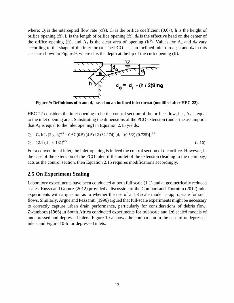
where: Qi is the intercepted flow rate (cfs), Co is the orifice coefficient (0.67), h is the height of
orifice opening (ft), L is the length of orifice opening (ft), do is the effective head on the center of
the orifice opening (ft), and Ag is the clear area of opening (ft2). Values for Ag and do vary
according to the shape of the inlet throat. The PCO uses an inclined inlet throat; h and do in this
case are shown in Figure 9, where di is the depth at the lip of the curb opening (ft).
Figure 9: Definitions of h and do based on an inclined inlet throat (modified after HEC-22).
HEC-22 considers the inlet opening to be the control section of the orifice-flow, i.e., Ag is equal
to the inlet opening area. Substituting the dimensions of the PCO extension (under the assumption
that Ag is equal to the inlet opening) in Equation 2.15 yields:
Qi = Co h L (2 g do)0.5 = 0.67 (0.5) (4.5) {2 (32.174) [di – (0.5/2) (0.725)]}0.5
Qi = 12.1 (di – 0.181)0.5 (2.16)
For a conventional inlet, the inlet-opening is indeed the control section of the orifice. However, in
the case of the extension of the PCO inlet, if the outlet of the extension (leading to the main bay)
acts as the control section, then Equation 2.15 requires modifications accordingly.
2.5 On Experiment Scaling
Laboratory experiments have been conducted at both full scale (1:1) and at geometrically reduced
scales. Russo and Gomez (2012) provided a discussion of the Comport and Thornton (2012) inlet
experiments with a question as to whether the use of a 1:3 scale model is appropriate for such
flows. Similarly, Argue and Pezzaniti (1996) argued that full-scale experiments might be necessary
to correctly capture urban drain performance, particularly for considerations of debris flow.
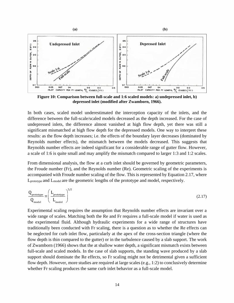
Zwamborn (1966) in South Africa conducted experiments for full-scale and 1:6 scaled models of
undepressed and depressed inlets. Figure 10-a shows the comparison in the case of undepressed
inlets and Figure 10-b for depressed inlets.
14
Figure 10: Comparison between full-scale and 1:6 scaled models: a) undepressed inlet, b)
depressed inlet (modified after Zwamborn, 1966).
In both cases, scaled model underestimated the interception capacity of the inlets, and the
difference between the full-scale/scaled models decreased as the depth increased. For the case of
undepressed inlets, the difference almost vanished at high flow depth, yet there was still a
significant mismatched at high flow depth for the depressed models. One way to interpret these
results: as the flow depth increases; i.e. the effects of the boundary layer decreases (dominated by
Reynolds number effects), the mismatch between the models decreased. This suggests that
Reynolds number effects are indeed significant for a considerable range of gutter flow. However,
a scale of 1:6 is quite small and may amplify the mismatch compared to larger 1:3 and 1:2 scales.
From dimensional analysis, the flow at a curb inlet should be governed by geometric parameters,
the Froude number (Fr), and the Reynolds number (Re). Geometric scaling of the experiments is
accompanied with Froude number scaling of the flow. This is represented by Equation 2.17, where
Lprototype and Lmodel are the geometric lengths of the prototype and model, respectively.
Qprototype
Qmodel
=L
prototype
Lmodel
æ
èç
ö
ø÷
5/2
(2.17)
Experimental scaling requires the assumption that Reynolds number effects are invariant over a
wide range of scales. Matching both the Re and Fr requires a full-scale model if water is used as
the experimental fluid. Although hydraulic experiments for a wide range of structures have
traditionally been conducted with Fr scaling, there is a question as to whether the Re effects can
be neglected for curb inlet flow, particularly at the apex of the cross-section triangle (where the
flow depth is thin compared to the gutter) or in the turbulence caused by a slab support. The work
of Zwamborn (1966) shows that the at shallow water depth, a significant mismatch exists between
full-scale and scaled models. In the case of slab supports, the standing wave produced by a slab
support should dominate the Re effects, so Fr scaling might not be detrimental given a sufficient
flow depth. However, more studies are required at large scales (e.g., 1:2) to conclusively determine
whether Fr scaling produces the same curb inlet behavior as a full-scale model.

15
2.6 Conclusions
Although curb inlets have continued to be studied, the focus over the past 20 years has largely
been on providing performance characteristics of specific inlets. Evidence of inlet/end wall effects
(see §2.3.2) supports the HEC-22 recommendation to avoid slab supports. However, slab supports
are a structural necessity for long inlets and cannot be simply dismissed as an inefficient or
unacceptable design practice. Unfortunately, there has been no attempt to develop a theoretical
model (i.e., similar to Izzard, 1950) to account for the presence of slab supports, nor has there been
any attempt to quantitatively investigate the effects of slab supports on inlet efficiency. The review
also showed a potential inaccuracy associated with using scaled models, especially at shallow
gutter flow. Although inlets with channel extensions has been widely use, the concerns regarding
potential flow restrictions in these inlets are yet to be addressed. This literature review has
confirmed the need to conduct the full-scale experimental investigations for TxDOT Project 0-
6842.

16
Chapter 3: Experimental Step-up
3.1 Existing Modeling Facility
The physical model is located in the CWE laboratory at the J.J. Pickle Research Campus of The
University of Texas at Austin. The physical model was originally constructed for Holley et al.
(1992), and built as a 3:4 scale representation of one lane of a roadway with adjustable longitudinal
and cross slopes. It has been used for a variety of projects (e.g. Hammond and Holley, 1995; Qian
et al., 2013) and modified according to projects’ specific needs.
The physical model has a length of 64 ft (19.05 m) and operational surface (framed by two curbs)
width of 10.5 ft (3.2 m). The physical model has a steel structure supporting a wood deck, curbs
and headbox. The steel structure is supported at 4 locations, each near a corner of the physical
model. One corner sits on a ball bearing, acting as a pivot point and allowing the other three corners
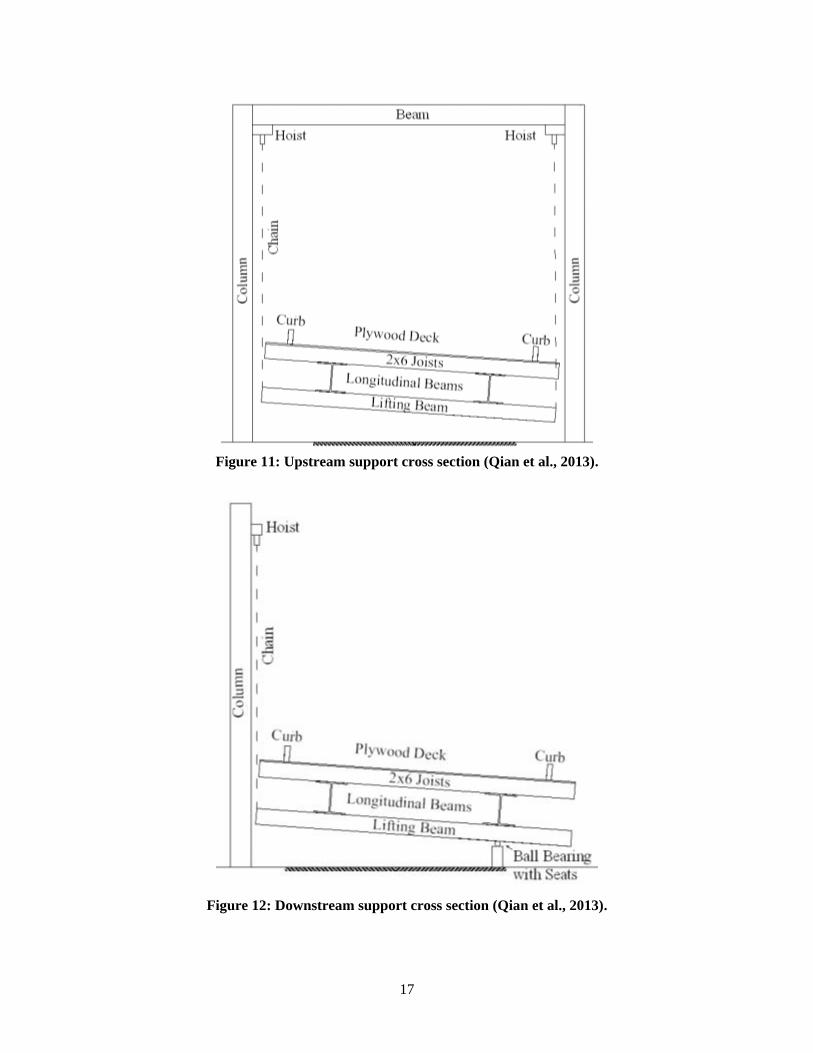
to be raised and lowered independently by crane hoists (Figure 11Figure 12). This provides a full
range of longitudinal and cross slope combinations. A 12 inch diameter pipe, reduced to 4 inch
pipe and valve, provides the water supply into a headbox at the upstream end of the physical model.
Water is taken from an exterior holding tank by 2 pumps operating in parallel. The pumps were
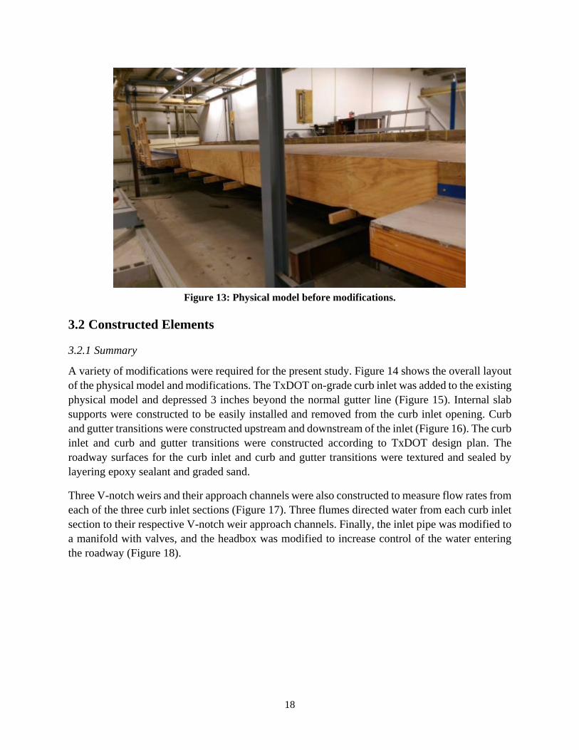
designed to discharge up to 7 cfs (Holley et al., 1992). Figure 13 shows the roadway before
modifications.
The model’s road surface is sealed with layers of fiberglass and resin. The surface is textured with
a mean diameter particle size of 1.3 mm (Hammond and Holley, 1995). Recent roughness
calculations performed by Qian et al. (2013) show an average Manning’s roughness coefficient of
0.0166.
17
Figure 11: Upstream support cross section (Qian et al., 2013).
Figure 12: Downstream support cross section (Qian et al., 2013).
18
Figure 13: Physical model before modifications.
3.2 Constructed Elements
3.2.1 Summary
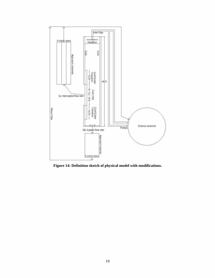
A variety of modifications were required for the present study. Figure 14 shows the overall layout
of the physical model and modifications. The TxDOT on-grade curb inlet was added to the existing
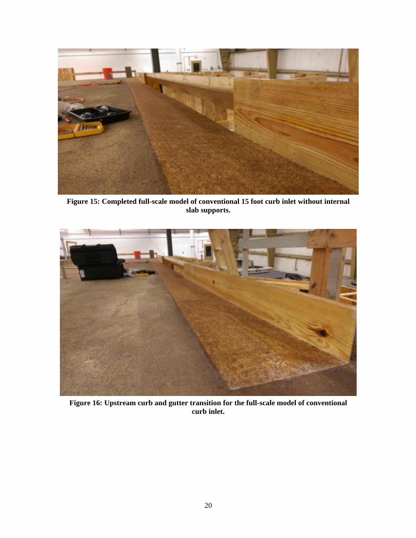
physical model and depressed 3 inches beyond the normal gutter line (Figure 15). Internal slab
supports were constructed to be easily installed and removed from the curb inlet opening. Curb
and gutter transitions were constructed upstream and downstream of the inlet (Figure 16). The curb
inlet and curb and gutter transitions were constructed according to TxDOT design plan. The
roadway surfaces for the curb inlet and curb and gutter transitions were textured and sealed by
layering epoxy sealant and graded sand.
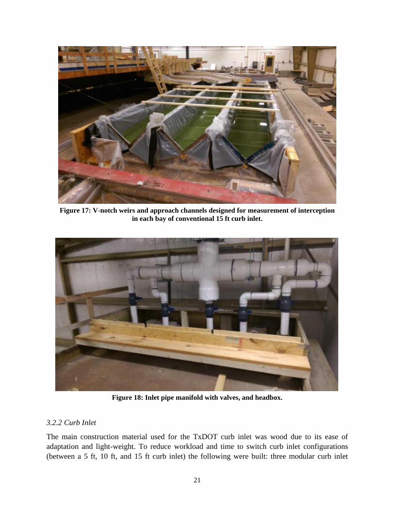
Three V-notch weirs and their approach channels were also constructed to measure flow rates from
each of the three curb inlet sections (Figure 17). Three flumes directed water from each curb inlet
section to their respective V-notch weir approach channels. Finally, the inlet pipe was modified to
a manifold with valves, and the headbox was modified to increase control of the water entering
the roadway (Figure 18).
19
Figure 14: Definition sketch of physical model with modifications.
20
Figure 15: Completed full-scale model of conventional 15 foot curb inlet without internal
slab supports.
Figure 16: Upstream curb and gutter transition for the full-scale model of conventional
curb inlet.
21
Figure 17: V-notch weirs and approach channels designed for measurement of interception
in each bay of conventional 15 ft curb inlet.
Figure 18: Inlet pipe manifold with valves, and headbox.
3.2.2 Curb Inlet
The main construction material used for the TxDOT curb inlet was wood due to its ease of
adaptation and light-weight. To reduce workload and time to switch curb inlet configurations
(between a 5 ft, 10 ft, and 15 ft curb inlet) the following were built: three modular curb inlet
22
sections (5 ft lengths), two removable flush slab supports, one modular curb and gutter transition
(downstream of the curb inlet), one permanent curb and gutter transition (upstream of the curb
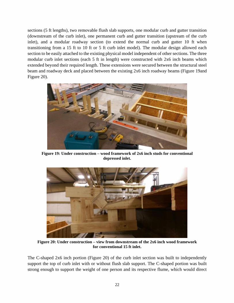
inlet), and a modular roadway section (to extend the normal curb and gutter 10 ft when
transitioning from a 15 ft to 10 ft or 5 ft curb inlet model). The modular design allowed each
section to be easily attached to the existing physical model independent of other sections. The three
modular curb inlet sections (each 5 ft in length) were constructed with 2x6 inch beams which
extended beyond their required length. These extensions were secured between the structural steel
beam and roadway deck and placed between the existing 2x6 inch roadway beams (Figure 19and
Figure 20).
Figure 19: Under construction – wood framework of 2x6 inch studs for conventional
depressed inlet.
Figure 20: Under construction – view from downstream of the 2x6 inch wood framework
for conventional 15 ft inlet.
The C-shaped 2x6 inch portion (Figure 20) of the curb inlet section was built to independently
support the top of curb inlet with or without flush slab support. The C-shaped portion was built
strong enough to support the weight of one person and its respective flume, which would direct
23
the curb inlet’s intercepted flow into an approach channel. On top of the 2x6 inch beams ¾ inch
plywood was installed.
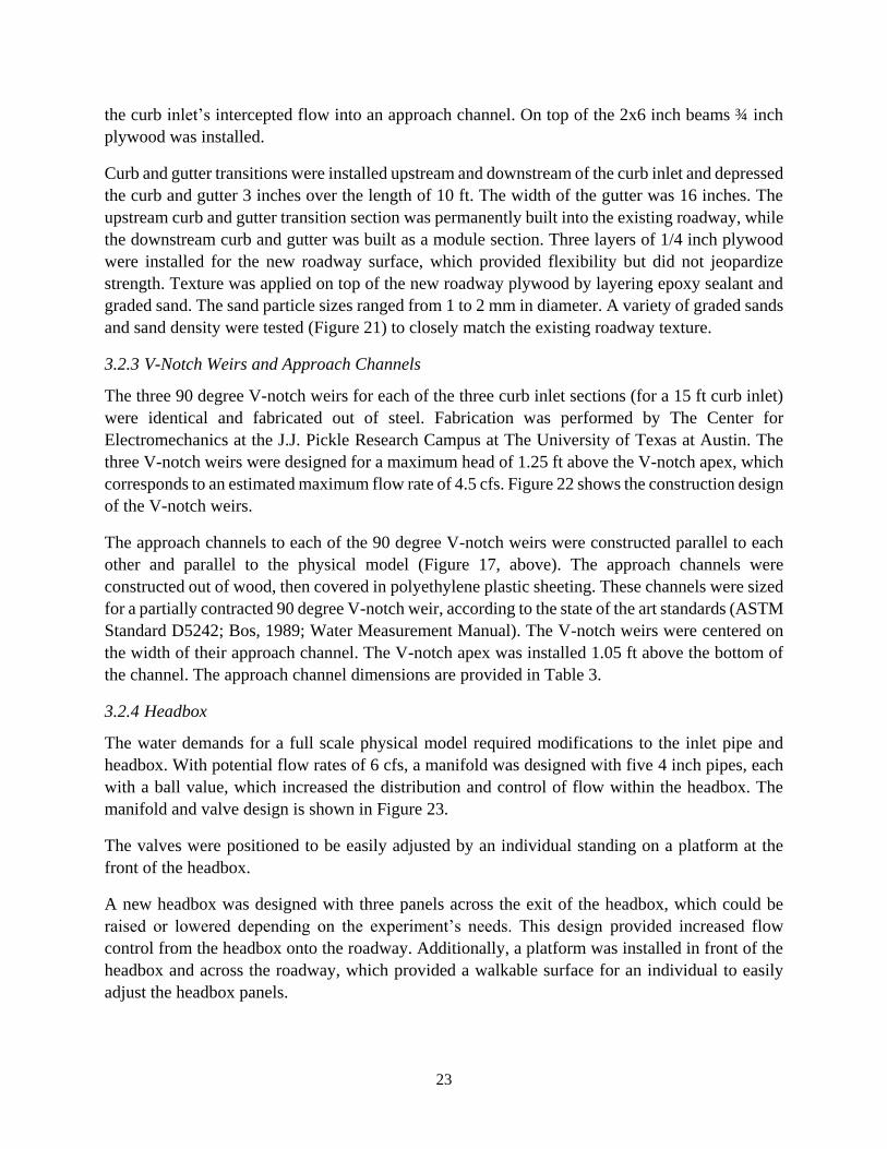
Curb and gutter transitions were installed upstream and downstream of the curb inlet and depressed
the curb and gutter 3 inches over the length of 10 ft. The width of the gutter was 16 inches. The
upstream curb and gutter transition section was permanently built into the existing roadway, while
the downstream curb and gutter was built as a module section. Three layers of 1/4 inch plywood
were installed for the new roadway surface, which provided flexibility but did not jeopardize
strength. Texture was applied on top of the new roadway plywood by layering epoxy sealant and
graded sand. The sand particle sizes ranged from 1 to 2 mm in diameter. A variety of graded sands
and sand density were tested (Figure 21) to closely match the existing roadway texture.
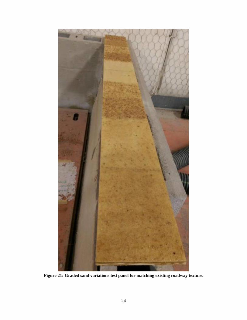
3.2.3 V-Notch Weirs and Approach Channels
The three 90 degree V-notch weirs for each of the three curb inlet sections (for a 15 ft curb inlet)
were identical and fabricated out of steel. Fabrication was performed by The Center for
Electromechanics at the J.J. Pickle Research Campus at The University of Texas at Austin. The
three V-notch weirs were designed for a maximum head of 1.25 ft above the V-notch apex, which
corresponds to an estimated maximum flow rate of 4.5 cfs. Figure 22 shows the construction design
of the V-notch weirs.
The approach channels to each of the 90 degree V-notch weirs were constructed parallel to each
other and parallel to the physical model (Figure 17, above). The approach channels were
constructed out of wood, then covered in polyethylene plastic sheeting. These channels were sized
for a partially contracted 90 degree V-notch weir, according to the state of the art standards (ASTM
Standard D5242; Bos, 1989; Water Measurement Manual). The V-notch weirs were centered on
the width of their approach channel. The V-notch apex was installed 1.05 ft above the bottom of
the channel. The approach channel dimensions are provided in Table 3.
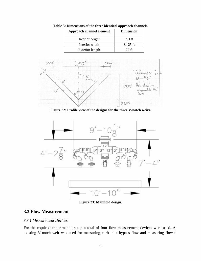
3.2.4 Headbox
The water demands for a full scale physical model required modifications to the inlet pipe and
headbox. With potential flow rates of 6 cfs, a manifold was designed with five 4 inch pipes, each
with a ball value, which increased the distribution and control of flow within the headbox. The
manifold and valve design is shown in Figure 23.
The valves were positioned to be easily adjusted by an individual standing on a platform at the
front of the headbox.
A new headbox was designed with three panels across the exit of the headbox, which could be
raised or lowered depending on the experiment’s needs. This design provided increased flow
control from the headbox onto the roadway. Additionally, a platform was installed in front of the
headbox and across the roadway, which provided a walkable surface for an individual to easily
adjust the headbox panels.
24
Figure 21: Graded sand variations test panel for matching existing roadway texture.
25
Table 3: Dimensions of the three identical approach channels.
Approach channel element Dimension
Interior height 2.3 ft
Interior width 3.125 ft
Exterior length 22 ft
Figure 22: Profile view of the designs for the three V-notch weirs.
Figure 23: Manifold design.
3.3 Flow Measurement
3.3.1 Measurement Devices
For the required experimental setup a total of four flow measurement devices were used. An
existing V-notch weir was used for measuring curb inlet bypass flow and measuring flow to

26
determining the Manning’s n. This weir was located at the bottom of the roadway and can be used
as either a 120 degree or 60 degree V-notch weir.
The three remaining flow measurement devices were 90 degree V-notch weirs. The V-notch weirs
were identical and fabricated out of steel. The three weirs were designed for a maximum head of
1.25 ft above the notch apex, which corresponds to an estimated maximum flow rate of 4.5 cfs.
The sizing of the weirs and their approach channels was done according to state of the art standards
(ASTM Standard D5242; Bos, 1989; U.S Department of the Interior).
3.3.2 Flow Equations
A V-notch weir flow rate can be calculated with as follows (Bos, 1989; ASTM Standard D5242):
5/2
e
8Q C 2g tan H
15 2
(3.1)
where Q is the discharge (cfs), Ce is the discharge coefficient (a factor of notch angle and
contraction type), is the angle of the V-notch weir (degrees), and H is the head on the weir
measured from the apex (ft). The three V-notch angles used were: 60, 90 and 120 degrees. The 60
degree V-notch weir was used to measure flow that bypassed the curb inlet. The 120 degree V-
notch weir was used to measure flow rates when calibrating the physical model roughness. Three
90 degree partially-contracted V-notch weirs were used for each of the three curb inlet sections.
The term partially-contracted is used when the sidewalls and bottom of the approach channel affect
the contraction of the jet of water flowing over the weir (ASTM Standard D5242). The partially-
contracted 90 degree V-notch weirs were not fully contracted due to space constraints in the
laboratory. Partial contraction of a 90 degree V-notch weir is an approved method and the
discharge coefficient uncertainty 1% compared to a fully-contracted weir.
For a 60 degree V-notch weir Ce = 0.577 (Figure 5.9 from Bos, 1989; Figure 6 from ASTM
Standard D5242) and Equation 3.1 becomes:
5/2Q 1.426H (3.2)
For a 90 degree partially contracted V-notch weir Ce = 0.597 (Figure 5.10 from Bos, 1989; Figure
7 from ASTM Standard D5242) and Equation 3.1 becomes:
5/2Q 2.555H (3.3)
For a 120 degree V-notch weir Ce = 0.584 (Grant and Dawson, 2001) and Equation 3.1 becomes:
5/2Q 4.330H (3.4)
The flow rate measurements were calculated with an ISCO 4230 Bubbler Flow Meter. This device
accurately measures head on a weir and is programmed to use Equations 3.2, 3.3, and 3.4 to
continuously output flow rates.

27
3.3.3 Flow Measurement Device Calibration
An Acoustic Doppler Velocimeter (ADV) is a device that measures point velocities. After a variety
of calibration tests it was determined that the ADV was not appropriate for the purpose of flow
measurement calibration in the outflow channels. Instead of using the ADV, a sharp crested
rectangular weir without end contractions was used. Furthermore, by using a rectangular weir that
is downstream of all four V-notch weirs, it was possible to compare the cumulative flow rate of
all four V-notch weirs to the rectangular weir.
A sharp crested rectangular weir flow rate can be calculated with the following equation (Grant
and Dawson, 2001):
1.5Q 3.330LH (3.5)
where Q is the discharge (cfs), L is the length of the weir, and H is the head on the weir measured
from the top of the weir (ft). With the weir length of 5 feet Equation 3.5 becomes
1.5Q 16.65H (3.6)
The flow measurement was calculated by measuring and averaging H from both sides of the
channel and using Equation 3.6. A range of 11 flow rates from 1 cfs to 6 cfs were measured for
the rectangular weir and all V-notch weirs. Figure 24 provides a comparison of flow rates for the
V-notch weirs and rectangular weir. The root mean square difference (RMSD) between the V-
notch weirs and rectangular weir was 0.36 cfs. The alignment between the V-notch weirs and
rectangular weir shows that the V-notch weir flow measurement devices are reasonable and
Equations 3.2 - 3.4 are appropriate.
Figure 24: Flow measurement calibration. Comparison of simultaneously measured flows
with the new V-notch weirs and the existing rectangular weir.

28
3.3.4 Uncertainty in Measurements
Measurement uncertainty is determined by adding the combined standard uncertainty (CSU) with
the flow rate variability from the Bubbler Flow Meter. The variability in flow rate from the Bubbler
Flow Meter is due to the natural undulation of water levels in the V-notch weir approach channel.
The CSU can be expressed as follows:
UQ,Equation= √(∂f
∂CeuCe
)2
+ (∂f
∂θuθ)
2
+ (∂f
∂HuH)
2
(3.7)
where UQ,Equation is the CSU of the V-notch weirs flow rate. The measured quantities Ce, θ, and H,
are functions of Equation 3.1, which have their own respective uncertainty (e.g. UH), which are
listed in Table 4. The UCe value of Equation 3.7 was selected from ASTM Standard D5242. The
UƟ value was estimated based on V-notch weir construction accuracy. The UH value was estimated
from the uncertainty in defining the water level datum compared to the apex of the V-notch. The
variability in flow rate outputs due to natural undulation in water levels can be expressed as
follows:
UQ,measured= 0.005Qmeasured + 0.005 (3.8)
where UQ,Measured is the uncertainty from the flow rate outputs and Qmeasured is the flow rate output
from the Bubbler Flow Meter.
Table 4: Individual uncertainty quantities in Equation 3.8.
Measured Quantities Unit of Measurement Uncertainty
Ce N/A ±0.0119
degree ±0.01
H feet ±0.00984
The total measured uncertainty (UT) is the summation of Equation 3.7 and 3.8 and is expressed in Equation
3.9 for a 15-foot curb inlet (upper bound of uncertainty) and Equation 3.10 for a 5-ft curb inlet (lower bound
of uncertainty). The total uncertainty ranges from ±0.03 cfs at Q=0.5 cfs for a 5-foot curb inlet to ±0.23 cfs
at Q=6cfs for a 15-foot curb inlet.
UT,15ft = 0.031Q + 0.0397 (3.9)
UT,5ft = 0.0256Q + 0.0216 (3.10)
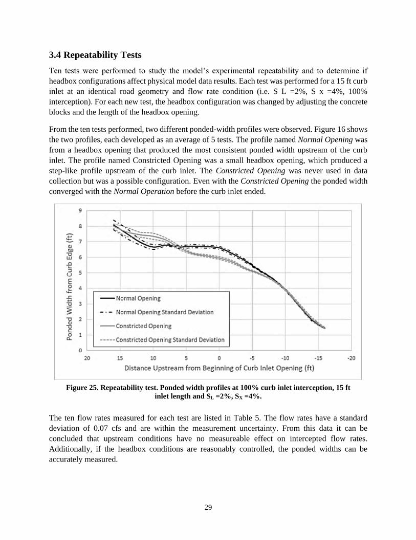
29
3.4 Repeatability Tests
Ten tests were performed to study the model’s experimental repeatability and to determine if
headbox configurations affect physical model data results. Each test was performed for a 15 ft curb
inlet at an identical road geometry and flow rate condition (i.e. S L =2%, S x =4%, 100%
interception). For each new test, the headbox configuration was changed by adjusting the concrete
blocks and the length of the headbox opening.
From the ten tests performed, two different ponded-width profiles were observed. Figure 16 shows
the two profiles, each developed as an average of 5 tests. The profile named Normal Opening was
from a headbox opening that produced the most consistent ponded width upstream of the curb
inlet. The profile named Constricted Opening was a small headbox opening, which produced a
step-like profile upstream of the curb inlet. The Constricted Opening was never used in data
collection but was a possible configuration. Even with the Constricted Opening the ponded width
converged with the Normal Operation before the curb inlet ended.
Figure 25. Repeatability test. Ponded width profiles at 100% curb inlet interception, 15 ft
inlet length and SL =2%, SX =4%.
The ten flow rates measured for each test are listed in Table 5. The flow rates have a standard
deviation of 0.07 cfs and are within the measurement uncertainty. From this data it can be
concluded that upstream conditions have no measureable effect on intercepted flow rates.
Additionally, if the headbox conditions are reasonably controlled, the ponded widths can be
accurately measured.
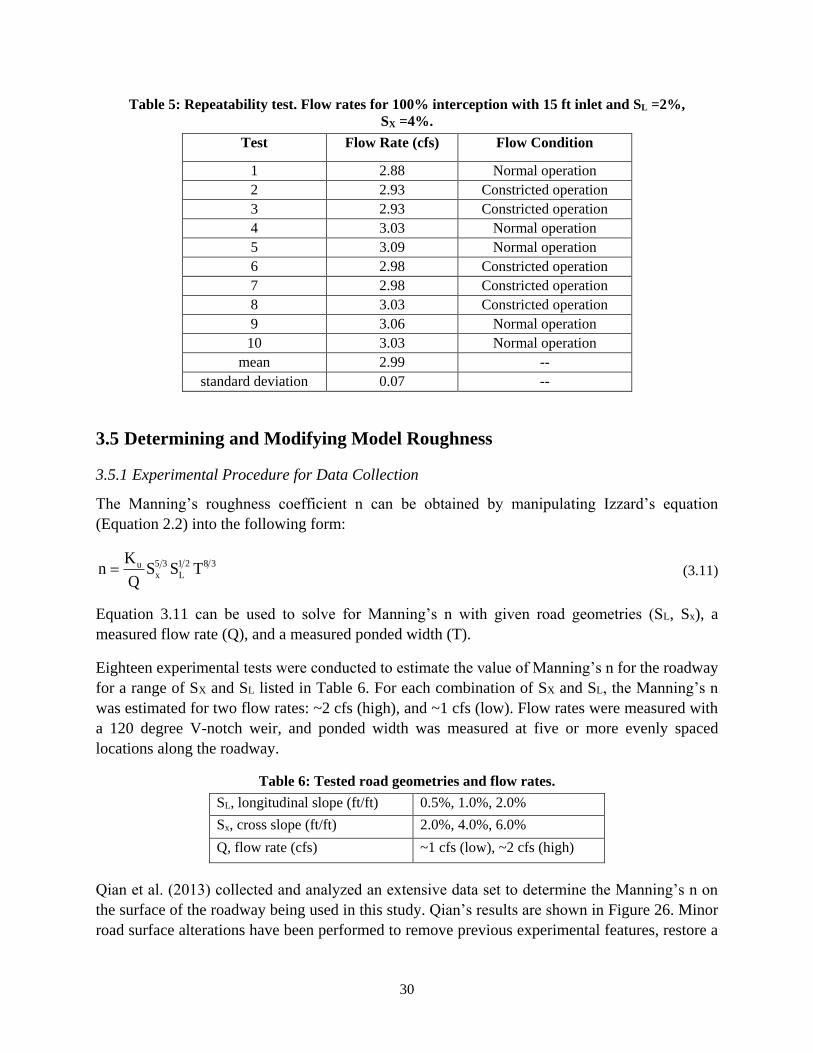
30
Table 5: Repeatability test. Flow rates for 100% interception with 15 ft inlet and SL =2%,
SX =4%.
Test Flow Rate (cfs) Flow Condition
1 2.88 Normal operation
2 2.93 Constricted operation
3 2.93 Constricted operation
4 3.03 Normal operation
5 3.09 Normal operation
6 2.98 Constricted operation
7 2.98 Constricted operation
8 3.03 Constricted operation
9 3.06 Normal operation
10 3.03 Normal operation
mean 2.99 --
standard deviation 0.07 --
3.5 Determining and Modifying Model Roughness
3.5.1 Experimental Procedure for Data Collection
The Manning’s roughness coefficient n can be obtained by manipulating Izzard’s equation
(Equation 2.2) into the following form:
5 3 1 2 8 3ux L
Kn S S T
Q (3.11)
Equation 3.11 can be used to solve for Manning’s n with given road geometries (SL, Sx), a
measured flow rate (Q), and a measured ponded width (T).
Eighteen experimental tests were conducted to estimate the value of Manning’s n for the roadway
for a range of SX and SL listed in Table 6. For each combination of SX and SL, the Manning’s n
was estimated for two flow rates: ~2 cfs (high), and ~1 cfs (low). Flow rates were measured with
a 120 degree V-notch weir, and ponded width was measured at five or more evenly spaced
locations along the roadway.
Table 6: Tested road geometries and flow rates.
SL, longitudinal slope (ft/ft) 0.5%, 1.0%, 2.0%
Sx, cross slope (ft/ft) 2.0%, 4.0%, 6.0%
Q, flow rate (cfs) ~1 cfs (low), ~2 cfs (high)
Qian et al. (2013) collected and analyzed an extensive data set to determine the Manning’s n on
the surface of the roadway being used in this study. Qian’s results are shown in Figure 26. Minor
road surface alterations have been performed to remove previous experimental features, restore a
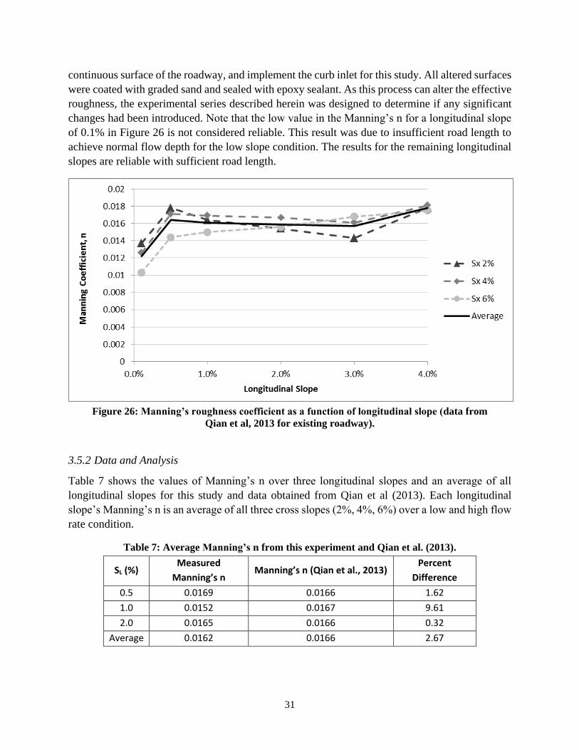
31
continuous surface of the roadway, and implement the curb inlet for this study. All altered surfaces
were coated with graded sand and sealed with epoxy sealant. As this process can alter the effective
roughness, the experimental series described herein was designed to determine if any significant
changes had been introduced. Note that the low value in the Manning’s n for a longitudinal slope
of 0.1% in Figure 26 is not considered reliable. This result was due to insufficient road length to
achieve normal flow depth for the low slope condition. The results for the remaining longitudinal
slopes are reliable with sufficient road length.
Figure 26: Manning’s roughness coefficient as a function of longitudinal slope (data from
Qian et al, 2013 for existing roadway).
3.5.2 Data and Analysis
Table 7 shows the values of Manning’s n over three longitudinal slopes and an average of all
longitudinal slopes for this study and data obtained from Qian et al (2013). Each longitudinal
slope’s Manning’s n is an average of all three cross slopes (2%, 4%, 6%) over a low and high flow
rate condition.
Table 7: Average Manning’s n from this experiment and Qian et al. (2013).
SL (%) Measured
Manning’s n Manning’s n (Qian et al., 2013)
Percent
Difference
0.5 0.0169 0.0166 1.62
1.0 0.0152 0.0167 9.61
2.0 0.0165 0.0166 0.32
Average 0.0162 0.0166 2.67

32
The average Manning’s n was determined to be 0.0162, a 2.67% difference from the Qian et al.
(2013) value of 0.0166. Experimental variation in data collection for the roadway typically ranges
from 1% to 10%, which encompasses the percent difference between this study and Qian et al.
(2013). The close alignment of data with Qian et al. (2013) confirms that the road surface
roughness has not significantly changed and that using their reported Manning’s n of 0.0166 for
this study is appropriate.
3.5.3 Roughness Modification
Once experiments were conducted on the original roughness of the roadway (n=0.0166),
resurfacing of the roadway was required to evaluate the impact of roughness on the curb inlet
performance. The final goal of the resurfacing process was to reach a smoother manning roughness
value of 0.012-0.013. During resurfacing, a total of four epoxy layers were applied on the roadway.
After each layer cured, testing was conducted to get an estimate of the Manning roughness value
thus decide whether to conduct full testing of the roughness value or apply additional epoxy layers.
When another epoxy layer was required, the surface of the road way was first roughened to ensure
mechanical bonding between the old and new epoxy layers.
18 tests were conducted to estimate the value of Manning’s n. For each combination of longitudinal
and cross-sectional slope, the Manning’s n was estimate for two flow rates: ~2 cfs (high), and ~1
cfs (low). Flow rates were measured with a 120 degree V-notch weir, and ponded width was
measured at nine evenly spaced locations along the roadway. Table 8 shows the values of
Manning’s n over three longitudinal slopes and an average of all longitudinal slopes. Each
longitudinal slope’s Manning’s n is an average of all three cross slopes (2%, 4%, 6%) for the low
and high flow rate conditions. The final estimated value of Manning’s roughness coefficient n after
resurfacing is 0.012.
Table 8: Measured values of Manning’s n after resurfacing the model.
SL (%) 0.5 1 2 Average
Measured Manning’s n 0.0127 0.0116 0.0116 0.012
3.6 Conclusions
An existing model of a roadway with adjustable slopes was modifying to accommodate a full-scale
model of depressed curb inlet. The modifications included 15 ft curb inlet consisting of three 5-ft
modular units, 10 ft upstream and downstream transition sections, a headbox for controlling flow
onto the model, V-notch weirs and approach channels for flow measurement. The uncertainty in
flow measurement was determined to be on average 5% of the flow measured. Repeatability tests
were conducted to ensure that the conditions at the upstream end of the model do not interfere with
the flow in the vicinity of the inlet. Finally, the original roughness of the model was quantified
(n=0.016), and after the testing of 5, 10, and 15 ft inlets was completed, the roadway of the model
was resurfaced using layers of epoxy to a obtain a smoother roadway (n=0.012).
33
Chapter 4: Effects of Slab Supports
4.1 Experimental Procedures for Data Collection
Conventional depressed inlets of 5, 10, and 15 ft were tested for various slope configurations
(Table 9). Two flow rate conditions were tested: 100% gutter flow rate interception by the curb
inlet (100% interception), and gutter bypass condition (or bypass) where less than 100% of the
gutter flow rate was intercepted by the curb inlet. To evaluate the effects of slab supports on the
interception capacity of inlets, the 10 and 15 ft inlets were tested with and without slab supports.
Table 9: Tested configurations for analysis of slab supports effects.
Property Tested
Longitudinal slope (%) 0.1, 0.5, 1.0, 2.0, 4.0
Cross slope (%) 2.0, 4.0, 6.0
Inlet configuration (inlet length/ number internal slab supports) 15/2, 15/0, 10/1, 10/0, 5/0
Flow Rate Conditions 100% interception, bypass
A single flow rate was determined for 100% interception by first slowly increasing the flow rate
until bypass flow was noticed. At this point the flow rate was slowly decreased until only a small
trickle of bypass flow was occurring. This instance was considered 100% interception.
Multiple bypass flow rates were collected and generally ranged from 0.1 to 0.5 cfs. A bypass flow
rate of up to 0.5 cfs is allowed by TxDOT and was selected as the upper limit. Bypass flow was
achieved by slowly increasing the flow rate until bypass flow occurs, then incrementally increasing
the flow rate to obtain the desired bypass flow rate. The range of bypass flow achieved was a
function of the pump capacity and physical model limitations (i.e. ponded width limit and water
depth at curb limit).
Once these conditions were met the following data were collected: flow rate(s), water spread, and
water depth. Flow rate measurements were taken from each V-notch weir and repeated after an
approximate 5-minute wait. This wait was to confirm the flow rate had not changed. If the flow
rate had changed another 5-minute wait occurred until a steady flow rate had occurred. Water
spread measurements were collected every 2 ft along the roadway, starting 18 ft upstream of the
beginning of the curb inlet opening and continued until 5 ft downstream of the end of the curb inlet
opening. Measurements were taken perpendicular to the curb from the curb edge to the edge of the
water surface on the roadway. Water depth was measured at 3 locations upstream of the gutter
depression transitions.
4.2 Results and Analysis
A total of 173 tests were conducted at the original roughness (n=0.0166) for the configurations
listed in Table 9. A summary of the conducted tests and the ranges of intercepted flow are provided
in Table 10.
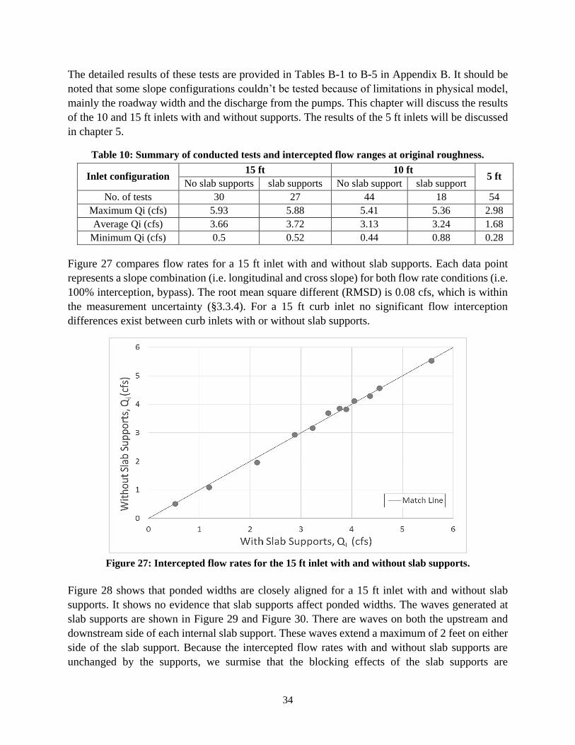
34
The detailed results of these tests are provided in Tables B-1 to B-5 in Appendix B. It should be
noted that some slope configurations couldn’t be tested because of limitations in physical model,
mainly the roadway width and the discharge from the pumps. This chapter will discuss the results
of the 10 and 15 ft inlets with and without supports. The results of the 5 ft inlets will be discussed
in chapter 5.
Table 10: Summary of conducted tests and intercepted flow ranges at original roughness.
Inlet configuration 15 ft 10 ft
5 ft No slab supports slab supports No slab support slab support
No. of tests 30 27 44 18 54
Maximum Qi (cfs) 5.93 5.88 5.41 5.36 2.98
Average Qi (cfs) 3.66 3.72 3.13 3.24 1.68
Minimum Qi (cfs) 0.5 0.52 0.44 0.88 0.28
Figure 27 compares flow rates for a 15 ft inlet with and without slab supports. Each data point
represents a slope combination (i.e. longitudinal and cross slope) for both flow rate conditions (i.e.
100% interception, bypass). The root mean square different (RMSD) is 0.08 cfs, which is within
the measurement uncertainty (§3.3.4). For a 15 ft curb inlet no significant flow interception
differences exist between curb inlets with or without slab supports.
Figure 27: Intercepted flow rates for the 15 ft inlet with and without slab supports.
Figure 28 shows that ponded widths are closely aligned for a 15 ft inlet with and without slab
supports. It shows no evidence that slab supports affect ponded widths. The waves generated at
slab supports are shown in Figure 29 and Figure 30. There are waves on both the upstream and
downstream side of each internal slab support. These waves extend a maximum of 2 feet on either
side of the slab support. Because the intercepted flow rates with and without slab supports are
unchanged by the supports, we surmise that the blocking effects of the slab supports are
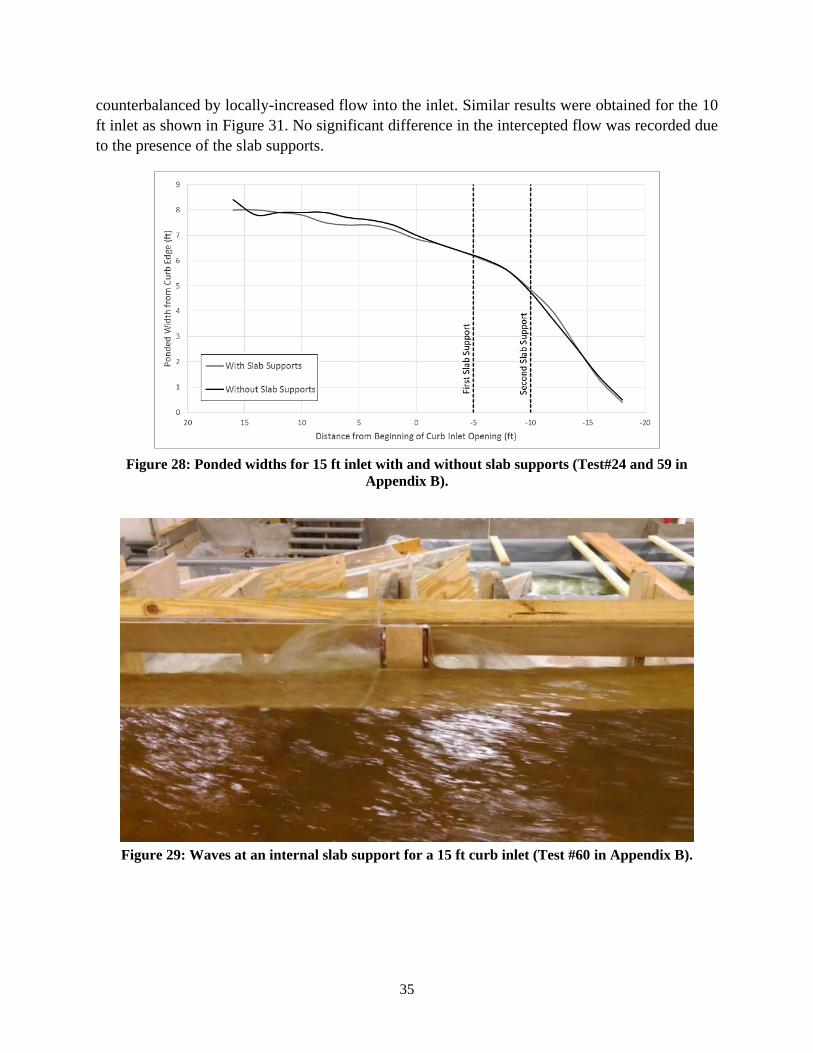
35
counterbalanced by locally-increased flow into the inlet. Similar results were obtained for the 10
ft inlet as shown in Figure 31. No significant difference in the intercepted flow was recorded due
to the presence of the slab supports.
Figure 28: Ponded widths for 15 ft inlet with and without slab supports (Test#24 and 59 in
Appendix B).
Figure 29: Waves at an internal slab support for a 15 ft curb inlet (Test #60 in Appendix B).
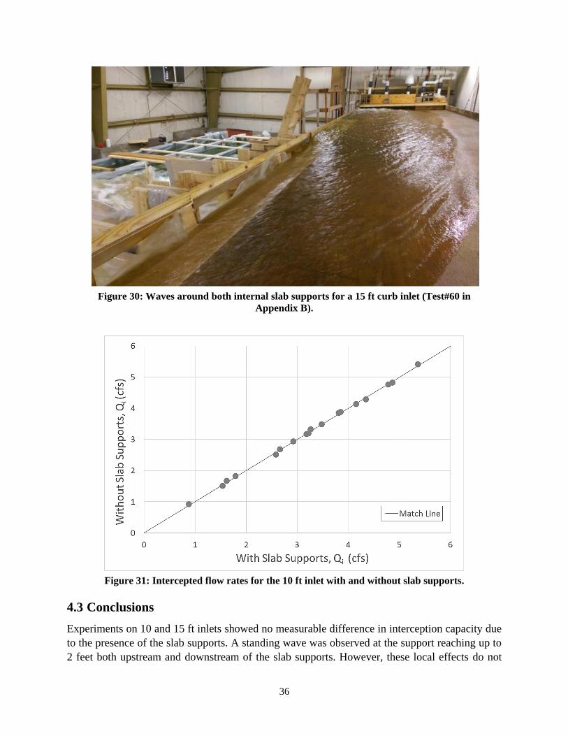
36
Figure 30: Waves around both internal slab supports for a 15 ft curb inlet (Test#60 in
Appendix B).
Figure 31: Intercepted flow rates for the 10 ft inlet with and without slab supports.
4.3 Conclusions
Experiments on 10 and 15 ft inlets showed no measurable difference in interception capacity due
to the presence of the slab supports. A standing wave was observed at the support reaching up to
2 feet both upstream and downstream of the slab supports. However, these local effects do not

37
affect the ponded width or the interception capacity of the inlet; flow obstructed by the supports is
simply diverted into the inlet upstream and/or downstream. Accordingly, the effective inlet length
should include the slab supports as well. In other words, to compute the effective inlet opening the
presence of the slab supports should be ignored and the length of the inlet be considered as the
distance from the upstream to the downstream ends of the curb opening (i.e., including the length
nominally blocked by the slab support as long as such blockage is sufficiently similar to the 6-inch
length of the tested slab supports).
These results indicate that the HEC-22 statement about slab supports reducing inlet capacity (see
§2.3.1) is incorrect. However, this should not be taken as proof that slab supports are irrelevant for
practical installation. We have not tested the effects of debris clogging, but can speculate on some
of the likely effects. The presence of slab supports arguably makes clogging more likely as large
debris (e.g., tree branches) can get caught on slab supports and collect additional debris. The effect
of such clogging would depend on whether 1 bay, 2 bays, or an entire 3-bay system is clogged.
Note that the PCO inlet extensions (see §2.4 and Chapter 6) will likely have increased clogging
due to the reduced area at the throat between the extension and the main basin.
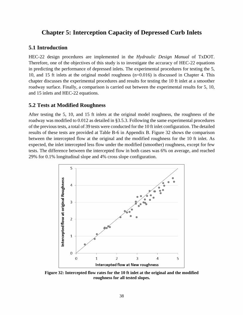
38
Chapter 5: Interception Capacity of Depressed Curb Inlets
5.1 Introduction
HEC-22 design procedures are implemented in the Hydraulic Design Manual of TxDOT.
Therefore, one of the objectives of this study is to investigate the accuracy of HEC-22 equations
in predicting the performance of depressed inlets. The experimental procedures for testing the 5,
10, and 15 ft inlets at the original model roughness (n=0.016) is discussed in Chapter 4. This
chapter discusses the experimental procedures and results for testing the 10 ft inlet at a smoother
roadway surface. Finally, a comparison is carried out between the experimental results for 5, 10,
and 15 inlets and HEC-22 equations.
5.2 Tests at Modified Roughness
After testing the 5, 10, and 15 ft inlets at the original model roughness, the roughness of the
roadway was modified to 0.012 as detailed in §3.5.3. Following the same experimental procedures
of the previous tests, a total of 39 tests were conducted for the 10 ft inlet configuration. The detailed
results of these tests are provided at Table B-6 in Appendix B. Figure 32 shows the comparison
between the intercepted flow at the original and the modified roughness for the 10 ft inlet. As
expected, the inlet intercepted less flow under the modified (smoother) roughness, except for few
tests. The difference between the intercepted flow in both cases was 6% on average, and reached
29% for 0.1% longitudinal slope and 4% cross slope configuration.
Figure 32: Intercepted flow rates for the 10 ft inlet at the original and the modified
roughness for all tested slopes.
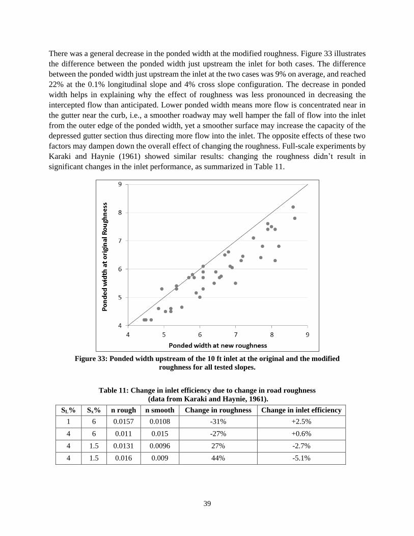
39
There was a general decrease in the ponded width at the modified roughness. Figure 33 illustrates
the difference between the ponded width just upstream the inlet for both cases. The difference
between the ponded width just upstream the inlet at the two cases was 9% on average, and reached
22% at the 0.1% longitudinal slope and 4% cross slope configuration. The decrease in ponded
width helps in explaining why the effect of roughness was less pronounced in decreasing the
intercepted flow than anticipated. Lower ponded width means more flow is concentrated near in
the gutter near the curb, i.e., a smoother roadway may well hamper the fall of flow into the inlet
from the outer edge of the ponded width, yet a smoother surface may increase the capacity of the
depressed gutter section thus directing more flow into the inlet. The opposite effects of these two
factors may dampen down the overall effect of changing the roughness. Full-scale experiments by
Karaki and Haynie (1961) showed similar results: changing the roughness didn’t result in
significant changes in the inlet performance, as summarized in Table 11.
Figure 33: Ponded width upstream of the 10 ft inlet at the original and the modified
roughness for all tested slopes.
Table 11: Change in inlet efficiency due to change in road roughness
(data from Karaki and Haynie, 1961).
SL% Sx% n rough n smooth Change in roughness Change in inlet efficiency
1 6 0.0157 0.0108 -31% +2.5%
4 6 0.011 0.015 -27% +0.6%
4 1.5 0.0131 0.0096 27% -2.7%
4 1.5 0.016 0.009 44% -5.1%
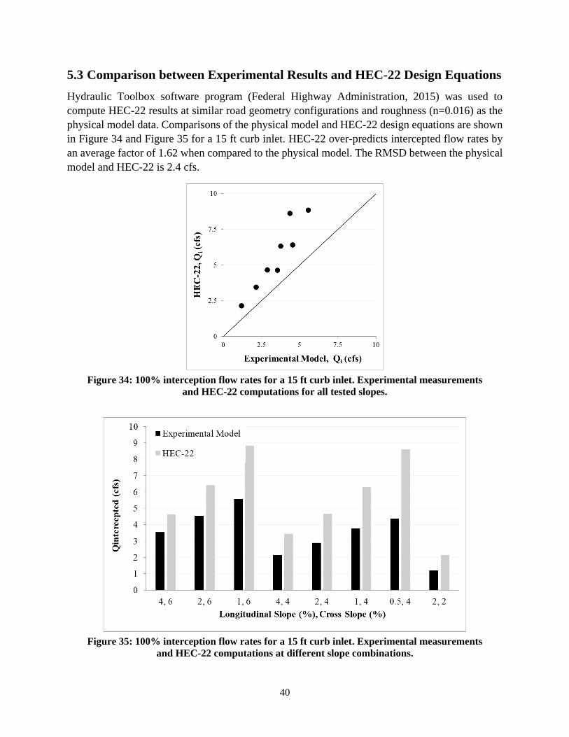
40
5.3 Comparison between Experimental Results and HEC-22 Design Equations
Hydraulic Toolbox software program (Federal Highway Administration, 2015) was used to
compute HEC-22 results at similar road geometry configurations and roughness (n=0.016) as the
physical model data. Comparisons of the physical model and HEC-22 design equations are shown
in Figure 34 and Figure 35 for a 15 ft curb inlet. HEC-22 over-predicts intercepted flow rates by
an average factor of 1.62 when compared to the physical model. The RMSD between the physical
model and HEC-22 is 2.4 cfs.
Figure 34: 100% interception flow rates for a 15 ft curb inlet. Experimental measurements
and HEC-22 computations for all tested slopes.
Figure 35: 100% interception flow rates for a 15 ft curb inlet. Experimental measurements
and HEC-22 computations at different slope combinations.
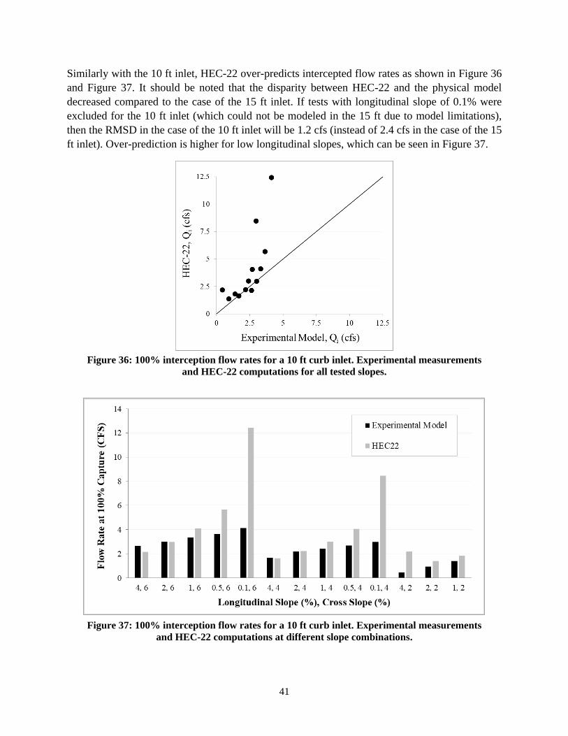
41
Similarly with the 10 ft inlet, HEC-22 over-predicts intercepted flow rates as shown in Figure 36
and Figure 37. It should be noted that the disparity between HEC-22 and the physical model
decreased compared to the case of the 15 ft inlet. If tests with longitudinal slope of 0.1% were
excluded for the 10 ft inlet (which could not be modeled in the 15 ft due to model limitations),
then the RMSD in the case of the 10 ft inlet will be 1.2 cfs (instead of 2.4 cfs in the case of the 15
ft inlet). Over-prediction is higher for low longitudinal slopes, which can be seen in Figure 37.
Figure 36: 100% interception flow rates for a 10 ft curb inlet. Experimental measurements
and HEC-22 computations for all tested slopes.
Figure 37: 100% interception flow rates for a 10 ft curb inlet. Experimental measurements
and HEC-22 computations at different slope combinations.
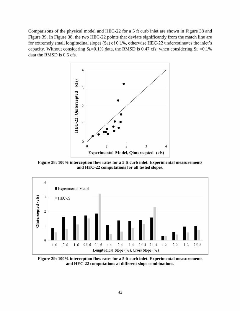
42
Comparisons of the physical model and HEC-22 for a 5 ft curb inlet are shown in Figure 38 and
Figure 39. In Figure 38, the two HEC-22 points that deviate significantly from the match line are
for extremely small longitudinal slopes (SL) of 0.1%, otherwise HEC-22 underestimates the inlet’s
capacity. Without considering SL=0.1% data, the RMSD is 0.47 cfs; when considering SL =0.1%
data the RMSD is 0.6 cfs.
Figure 38: 100% interception flow rates for a 5 ft curb inlet. Experimental measurements
and HEC-22 computations for all tested slopes.
Figure 39: 100% interception flow rates for a 5 ft curb inlet. Experimental measurements
and HEC-22 computations at different slope combinations.
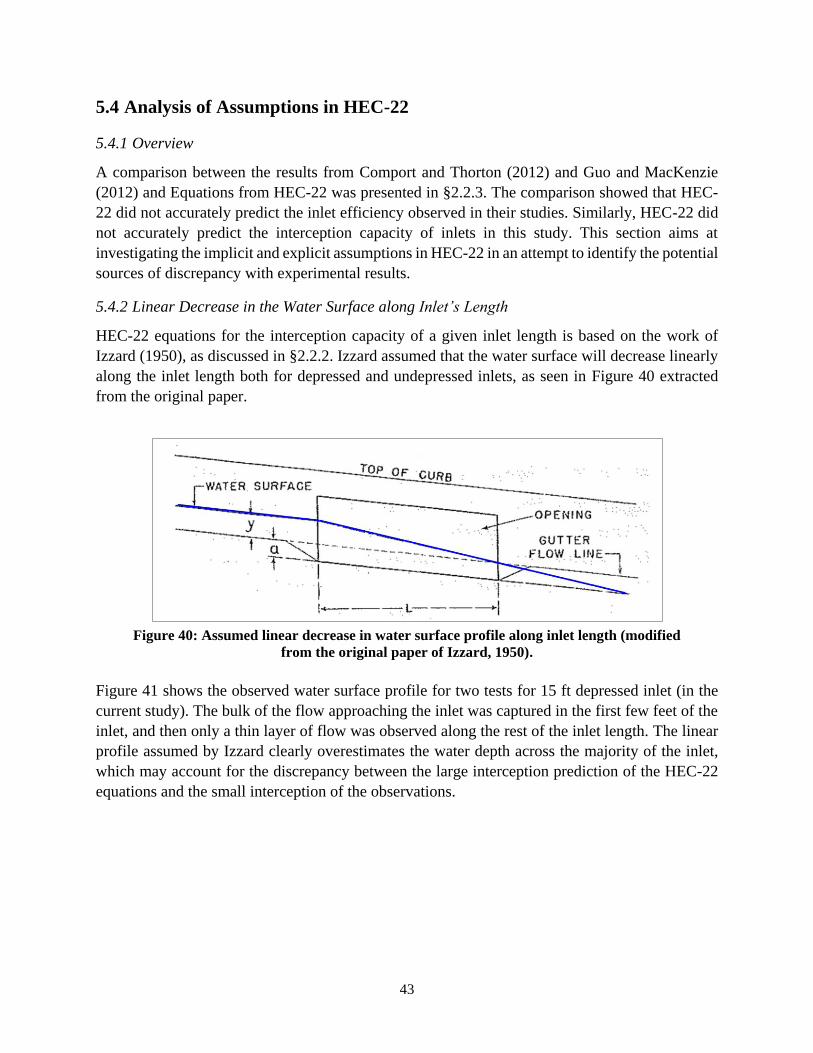
43
5.4 Analysis of Assumptions in HEC-22
5.4.1 Overview
A comparison between the results from Comport and Thorton (2012) and Guo and MacKenzie
(2012) and Equations from HEC-22 was presented in §2.2.3. The comparison showed that HEC-
22 did not accurately predict the inlet efficiency observed in their studies. Similarly, HEC-22 did
not accurately predict the interception capacity of inlets in this study. This section aims at
investigating the implicit and explicit assumptions in HEC-22 in an attempt to identify the potential
sources of discrepancy with experimental results.
5.4.2 Linear Decrease in the Water Surface along Inlet’s Length
HEC-22 equations for the interception capacity of a given inlet length is based on the work of
Izzard (1950), as discussed in §2.2.2. Izzard assumed that the water surface will decrease linearly
along the inlet length both for depressed and undepressed inlets, as seen in Figure 40 extracted
from the original paper.
Figure 40: Assumed linear decrease in water surface profile along inlet length (modified
from the original paper of Izzard, 1950).
Figure 41 shows the observed water surface profile for two tests for 15 ft depressed inlet (in the
current study). The bulk of the flow approaching the inlet was captured in the first few feet of the
inlet, and then only a thin layer of flow was observed along the rest of the inlet length. The linear
profile assumed by Izzard clearly overestimates the water depth across the majority of the inlet,
which may account for the discrepancy between the large interception prediction of the HEC-22
equations and the small interception of the observations.
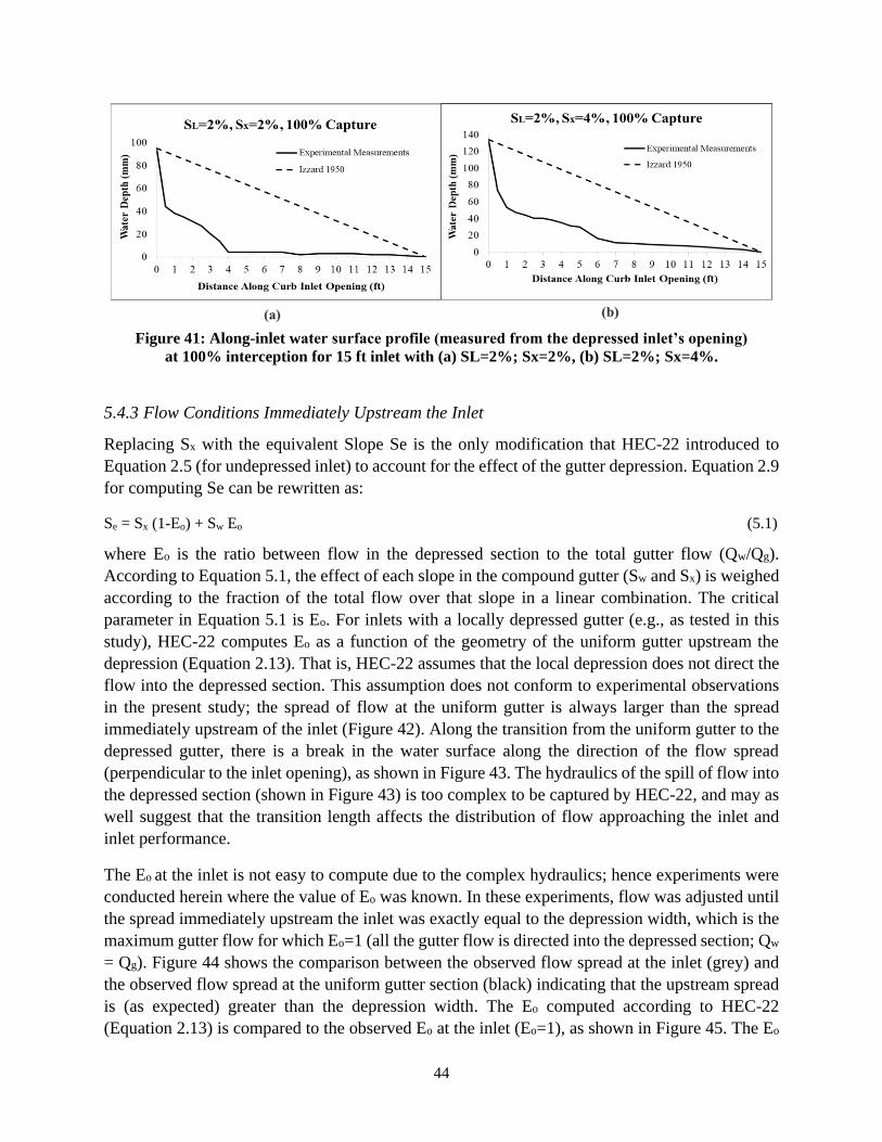
44
Figure 41: Along-inlet water surface profile (measured from the depressed inlet’s opening)
at 100% interception for 15 ft inlet with (a) SL=2%; Sx=2%, (b) SL=2%; Sx=4%.
5.4.3 Flow Conditions Immediately Upstream the Inlet
Replacing Sx with the equivalent Slope Se is the only modification that HEC-22 introduced to
Equation 2.5 (for undepressed inlet) to account for the effect of the gutter depression. Equation 2.9
for computing Se can be rewritten as:
Se = Sx (1-Eo) + Sw Eo (5.1)
where Eo is the ratio between flow in the depressed section to the total gutter flow (Qw/Qg).
According to Equation 5.1, the effect of each slope in the compound gutter (Sw and Sx) is weighed
according to the fraction of the total flow over that slope in a linear combination. The critical
parameter in Equation 5.1 is Eo. For inlets with a locally depressed gutter (e.g., as tested in this
study), HEC-22 computes Eo as a function of the geometry of the uniform gutter upstream the
depression (Equation 2.13). That is, HEC-22 assumes that the local depression does not direct the
flow into the depressed section. This assumption does not conform to experimental observations
in the present study; the spread of flow at the uniform gutter is always larger than the spread
immediately upstream of the inlet (Figure 42). Along the transition from the uniform gutter to the
depressed gutter, there is a break in the water surface along the direction of the flow spread
(perpendicular to the inlet opening), as shown in Figure 43. The hydraulics of the spill of flow into
the depressed section (shown in Figure 43) is too complex to be captured by HEC-22, and may as
well suggest that the transition length affects the distribution of flow approaching the inlet and
inlet performance.
The Eo at the inlet is not easy to compute due to the complex hydraulics; hence experiments were
conducted herein where the value of Eo was known. In these experiments, flow was adjusted until
the spread immediately upstream the inlet was exactly equal to the depression width, which is the
maximum gutter flow for which Eo=1 (all the gutter flow is directed into the depressed section; Qw
= Qg). Figure 44 shows the comparison between the observed flow spread at the inlet (grey) and
the observed flow spread at the uniform gutter section (black) indicating that the upstream spread
is (as expected) greater than the depression width. The Eo computed according to HEC-22
(Equation 2.13) is compared to the observed Eo at the inlet (Eo=1), as shown in Figure 45. The Eo
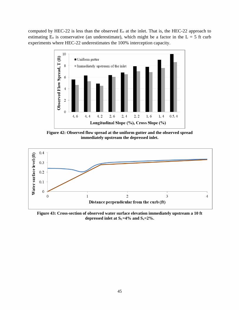
45
computed by HEC-22 is less than the observed Eo at the inlet. That is, the HEC-22 approach to
estimating Eo is conservative (an underestimate), which might be a factor in the L = 5 ft curb
experiments where HEC-22 underestimates the 100% interception capacity.
Figure 42: Observed flow spread at the uniform gutter and the observed spread
immediately upstream the depressed inlet.
Figure 43: Cross-section of observed water surface elevation immediately upstream a 10 ft
depressed inlet at SL=4% and Sx=2%.
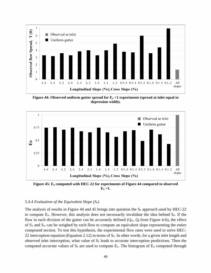
46
Figure 44: Observed uniform gutter spread for Eo =1 experiments (spread at inlet equal to
depression width).
Figure 45: Eo computed with HEC-22 for experiments of Figure 44 compared to observed
Eo =1.
5.4.4 Evaluation of the Equivalent Slope (Se)
The analysis of results in Figure 44 and 45 brings into question the Se approach used by HEC-22
to compute Eo. However, this analysis does not necessarily invalidate the idea behind Se. If the
flow in each division of the gutter can be accurately defined (Qw, Qs from Figure 4-b), the effect
of Sx and Sw can be weighed by each flow to compute an equivalent slope representing the entire
compound section. To test this hypothesis, the experimental flow rates were used to solve HEC-
22 interception equation (Equation 2.12) in terms of Se. In other words, for a given inlet length and
observed inlet interception, what value of Se leads to accurate interception predictions. Then the
computed accurate values of Se are used to compute Eo. The histogram of Eo computed through
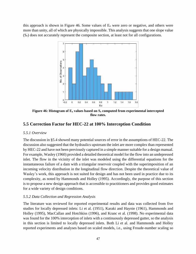
47
this approach is shown in Figure 46. Some values of Eo were zero or negative, and others were
more than unity, all of which are physically impossible. This analysis suggests that one slope value
(Se) does not accurately represent the composite section, at least not for all configurations.
Figure 46: Histogram of Eo values based on Se computed from experimental intercepted
flow rates.
5.5 Correction Factor for HEC-22 at 100% Interception Condition
5.5.1 Overview
The discussion in §5.4 showed many potential sources of error in the assumptions of HEC-22. The
discussion also suggested that the hydraulics upstream the inlet are more complex than represented
by HEC-22 and have not been previously captured in a simple manner suitable for a design manual.
For example, Wasley (1960) provided a detailed theoretical model for the flow into an undepressed
inlet. The flow in the vicinity of the inlet was modeled using the differential equations for the
instantaneous failure of a dam with a triangular reservoir coupled with the superimposition of an
incoming velocity distribution in the longitudinal flow direction. Despite the theoretical value of
Wasley’s work, this approach is not suited for design and has not been used in practice due to its
complexity, as noted by Hammonds and Holley (1995). Accordingly, the purpose of this section
is to propose a new design approach that is accessible to practitioners and provides good estimates
for a wide variety of design conditions.
5.5.2 Data Collection and Regression Analysis
The literature was reviewed for reported experimental results and data was collected from five
studies for locally depressed inlets: Li et al. (1951), Karaki and Haynie (1961), Hammonds and
Holley (1995), MacCallan and Hotchkiss (1996), and Kranc et al. (1998). No experimental data
was found for the 100% interception of inlets with a continuously depressed gutter, so the analysis
in this section is limited to locally depressed inlets. Both Li et al. and Hammonds and Holley
reported experiments and analyses based on scaled models, i.e., using Froude-number scaling so
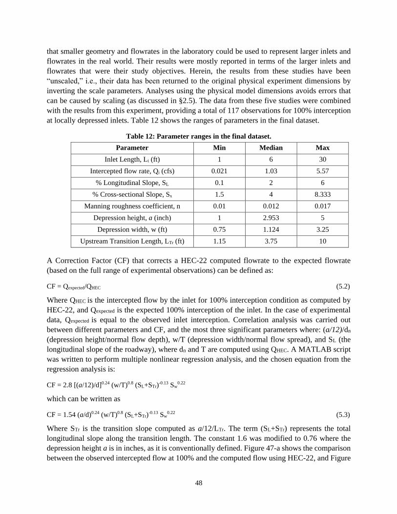
48
that smaller geometry and flowrates in the laboratory could be used to represent larger inlets and
flowrates in the real world. Their results were mostly reported in terms of the larger inlets and
flowrates that were their study objectives. Herein, the results from these studies have been
“unscaled,” i.e., their data has been returned to the original physical experiment dimensions by
inverting the scale parameters. Analyses using the physical model dimensions avoids errors that
can be caused by scaling (as discussed in §2.5). The data from these five studies were combined
with the results from this experiment, providing a total of 117 observations for 100% interception
at locally depressed inlets. Table 12 shows the ranges of parameters in the final dataset.
Table 12: Parameter ranges in the final dataset.
Parameter Min Median Max
Inlet Length, Li (ft) 1 6 30
Intercepted flow rate, Qi (cfs) 0.021 1.03 5.57
% Longitudinal Slope, SL 0.1 2 6
% Cross-sectional Slope, Sx 1.5 4 8.333
Manning roughness coefficient, n 0.01 0.012 0.017
Depression height, a (inch) 1 2.953 5
Depression width, w (ft) 0.75 1.124 3.25
Upstream Transition Length, LTr (ft) 1.15 3.75 10
A Correction Factor (CF) that corrects a HEC-22 computed flowrate to the expected flowrate
(based on the full range of experimental observations) can be defined as:
CF = Qexpected/QHEC (5.2)
Where QHEC is the intercepted flow by the inlet for 100% interception condition as computed by
HEC-22, and Qexpected is the expected 100% interception of the inlet. In the case of experimental
data, Qexpected is equal to the observed inlet interception. Correlation analysis was carried out
between different parameters and CF, and the most three significant parameters where: (a/12)/dn
(depression height/normal flow depth), w/T (depression width/normal flow spread), and SL (the
longitudinal slope of the roadway), where dn and T are computed using QHEC. A MATLAB script
was written to perform multiple nonlinear regression analysis, and the chosen equation from the
regression analysis is:
CF = 2.8 [(a/12)/d]0.24 (w/T)0.8 (SL+STr)-0.13 Sw
0.22
which can be written as
CF = 1.54 (a/d)0.24 (w/T)0.8 (SL+STr)-0.13 Sw
0.22 (5.3)
Where STr is the transition slope computed as a/12/LTr. The term (SL+STr) represents the total
longitudinal slope along the transition length. The constant 1.6 was modified to 0.76 where the
depression height a is in inches, as it is conventionally defined. Figure 47-a shows the comparison
between the observed intercepted flow at 100% and the computed flow using HEC-22, and Figure
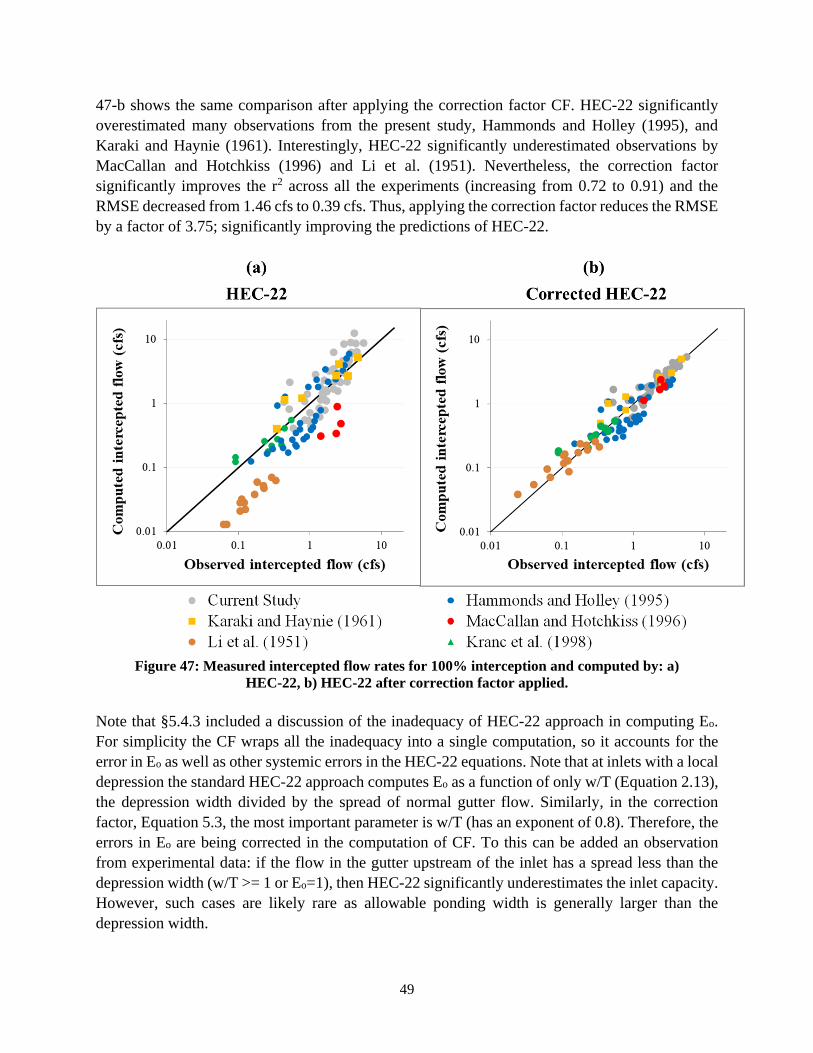
49
47-b shows the same comparison after applying the correction factor CF. HEC-22 significantly
overestimated many observations from the present study, Hammonds and Holley (1995), and
Karaki and Haynie (1961). Interestingly, HEC-22 significantly underestimated observations by
MacCallan and Hotchkiss (1996) and Li et al. (1951). Nevertheless, the correction factor
significantly improves the r2 across all the experiments (increasing from 0.72 to 0.91) and the
RMSE decreased from 1.46 cfs to 0.39 cfs. Thus, applying the correction factor reduces the RMSE
by a factor of 3.75; significantly improving the predictions of HEC-22.
Figure 47: Measured intercepted flow rates for 100% interception and computed by: a)
HEC-22, b) HEC-22 after correction factor applied.
Note that §5.4.3 included a discussion of the inadequacy of HEC-22 approach in computing Eo.
For simplicity the CF wraps all the inadequacy into a single computation, so it accounts for the
error in Eo as well as other systemic errors in the HEC-22 equations. Note that at inlets with a local
depression the standard HEC-22 approach computes Eo as a function of only w/T (Equation 2.13),
the depression width divided by the spread of normal gutter flow. Similarly, in the correction
factor, Equation 5.3, the most important parameter is w/T (has an exponent of 0.8). Therefore, the
errors in Eo are being corrected in the computation of CF. To this can be added an observation
from experimental data: if the flow in the gutter upstream of the inlet has a spread less than the
depression width (w/T >= 1 or Eo=1), then HEC-22 significantly underestimates the inlet capacity.
However, such cases are likely rare as allowable ponding width is generally larger than the
depression width.

50
The new design procedure can be summarized in the following steps:
Given input: Li, Sx, SL, STr, n, w, a
1) Compute the flow rate for 100% interception condition (QHEC) per instructions in HEC-22
(e.g. Hydraulic Toolbox software by the Federal Highway Administration, 2015)
2) Using the computed QHEC , compute T (spread of normal flow) using manning formula for
gutter flow by manipulating Equation 2.2:
T = (QHEC n
0.56√SL )
3/8
Sx−5/8
(5.4)
3) Compute dn:
dn = T Sx (5.5)
4) Compute a/dn and w/T, then apply Equation 5.3 (Note: depression height a is in inches).
5) Qexpected is then given by:
Qexpected = CF QHEC (5.6)
If flow in the gutter (Qg) is given and the required is to determine the inlet length for 100%
interception, then an iterative procedure is given in the following steps:
A) Assume Li, recommended to start with a small length (e.g., 1 ft)
B) Perform steps 1-5, above for computing Qexpected
C) Compute difference between given Qg and computed Qexpected as Qg - Qexpected
D) If Qg > Qexpected (difference is positive), assume large Li and repeat steps A-C, if Qg <
Qexpected then assume a smaller Li and repeat steps A-C till the difference become
insignificant. Table 13 provides an example of the iterative process.
Table 13: Iterative procedure to compute the 100% interception inlet length given the
gutter flow.
Input
a (inch) w (ft) Qg (cfs) SL% Sx% n STr % Li (ft) as a
check 3 1.333 3.64 0.5 6 0.0166 2.5 10
Iterations
Li (ft) QHEC (cfs) T (ft) dn (ft) a/dn w/T Qexpected (cfs) Diff%
1 0.06 1.46 0.088 34.25 1.747 0.23 93.61
5 1.56 4.95 0.3 10.1 0.444 1.7 53.3
8 3.81 6.92 0.42 7.23 0.269 2.93 19.49
11 7 8.69 0.52 5.75 0.236 4.25 -16.72
9.7 5.52 7.95 0.48 6.29 0.256 3.67 -0.97
5.5.3 Deficiency of Curb Inlets on a Combination of Steep Grade and Flat Cross Slope
During experiments for inlets at 4% SL and 2% Sx configuration, flow tended to go past the inlet
along the outer edge of the gutter. The 100% interception condition for this configuration was
barely achievable for both rough and smooth roadway surfaces. In the work of Hammonds and
Holley (1995), this tendency of the flow to move in the longitudinal direction and bypass the inlet
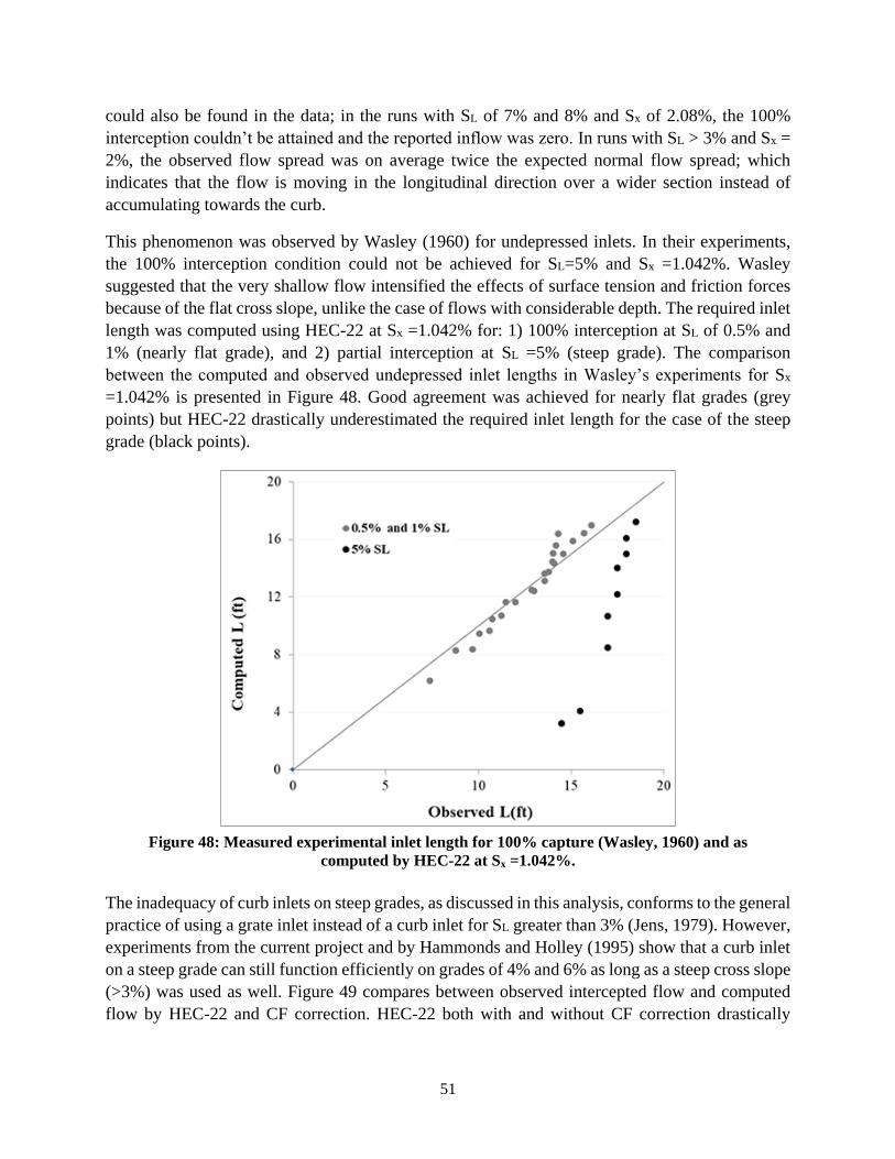
51
could also be found in the data; in the runs with SL of 7% and 8% and Sx of 2.08%, the 100%
interception couldn’t be attained and the reported inflow was zero. In runs with SL > 3% and Sx =
2%, the observed flow spread was on average twice the expected normal flow spread; which
indicates that the flow is moving in the longitudinal direction over a wider section instead of
accumulating towards the curb.
This phenomenon was observed by Wasley (1960) for undepressed inlets. In their experiments,
the 100% interception condition could not be achieved for SL=5% and Sx =1.042%. Wasley
suggested that the very shallow flow intensified the effects of surface tension and friction forces
because of the flat cross slope, unlike the case of flows with considerable depth. The required inlet
length was computed using HEC-22 at Sx =1.042% for: 1) 100% interception at SL of 0.5% and
1% (nearly flat grade), and 2) partial interception at SL =5% (steep grade). The comparison
between the computed and observed undepressed inlet lengths in Wasley’s experiments for Sx
=1.042% is presented in Figure 48. Good agreement was achieved for nearly flat grades (grey
points) but HEC-22 drastically underestimated the required inlet length for the case of the steep
grade (black points).
Figure 48: Measured experimental inlet length for 100% capture (Wasley, 1960) and as
computed by HEC-22 at Sx =1.042%.
The inadequacy of curb inlets on steep grades, as discussed in this analysis, conforms to the general
practice of using a grate inlet instead of a curb inlet for SL greater than 3% (Jens, 1979). However,
experiments from the current project and by Hammonds and Holley (1995) show that a curb inlet
on a steep grade can still function efficiently on grades of 4% and 6% as long as a steep cross slope
(>3%) was used as well. Figure 49 compares between observed intercepted flow and computed
flow by HEC-22 and CF correction. HEC-22 both with and without CF correction drastically
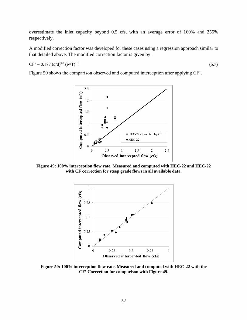
52
overestimate the inlet capacity beyond 0.5 cfs, with an average error of 160% and 255%
respectively.
A modified correction factor was developed for these cases using a regression approach similar to
that detailed above. The modified correction factor is given by:
CF’ = 0.177 (a/d)0.8 (w/T)1.18 (5.7)
Figure 50 shows the comparison observed and computed interception after applying CF’.
Figure 49: 100% interception flow rate. Measured and computed with HEC-22 and HEC-22
with CF correction for steep grade flows in all available data.
Figure 50: 100% interception flow rate. Measured and computed with HEC-22 with the
CF’ Correction for comparison with Figure 49.
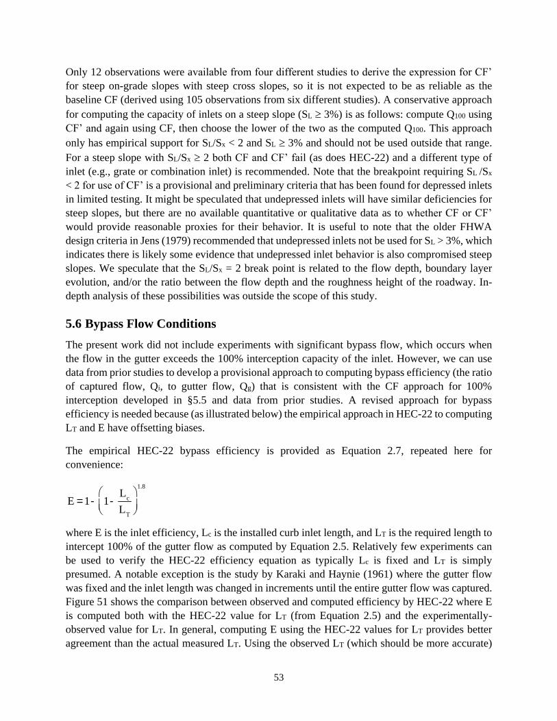
53
Only 12 observations were available from four different studies to derive the expression for CF’
for steep on-grade slopes with steep cross slopes, so it is not expected to be as reliable as the
baseline CF (derived using 105 observations from six different studies). A conservative approach
for computing the capacity of inlets on a steep slope (SL 3%) is as follows: compute Q100 using
CF’ and again using CF, then choose the lower of the two as the computed Q100. This approach
only has empirical support for SL/Sx < 2 and SL 3% and should not be used outside that range.
For a steep slope with SL/Sx 2 both CF and CF’ fail (as does HEC-22) and a different type of
inlet (e.g., grate or combination inlet) is recommended. Note that the breakpoint requiring SL /Sx
< 2 for use of CF’ is a provisional and preliminary criteria that has been found for depressed inlets
in limited testing. It might be speculated that undepressed inlets will have similar deficiencies for
steep slopes, but there are no available quantitative or qualitative data as to whether CF or CF’
would provide reasonable proxies for their behavior. It is useful to note that the older FHWA
design criteria in Jens (1979) recommended that undepressed inlets not be used for SL > 3%, which
indicates there is likely some evidence that undepressed inlet behavior is also compromised steep
slopes. We speculate that the SL/Sx = 2 break point is related to the flow depth, boundary layer
evolution, and/or the ratio between the flow depth and the roughness height of the roadway. In-
depth analysis of these possibilities was outside the scope of this study.
5.6 Bypass Flow Conditions
The present work did not include experiments with significant bypass flow, which occurs when
the flow in the gutter exceeds the 100% interception capacity of the inlet. However, we can use
data from prior studies to develop a provisional approach to computing bypass efficiency (the ratio
of captured flow, Qi, to gutter flow, Qg) that is consistent with the CF approach for 100%
interception developed in §5.5 and data from prior studies. A revised approach for bypass
efficiency is needed because (as illustrated below) the empirical approach in HEC-22 to computing
LT and E have offsetting biases.
The empirical HEC-22 bypass efficiency is provided as Equation 2.7, repeated here for
convenience:
E = 1- 1-L
c
LT
æ
èç
ö
ø÷
1.8
where E is the inlet efficiency, Lc is the installed curb inlet length, and LT is the required length to
intercept 100% of the gutter flow as computed by Equation 2.5. Relatively few experiments can
be used to verify the HEC-22 efficiency equation as typically Lc is fixed and LT is simply
presumed. A notable exception is the study by Karaki and Haynie (1961) where the gutter flow
was fixed and the inlet length was changed in increments until the entire gutter flow was captured.
Figure 51 shows the comparison between observed and computed efficiency by HEC-22 where E
is computed both with the HEC-22 value for LT (from Equation 2.5) and the experimentally-
observed value for LT. In general, computing E using the HEC-22 values for LT provides better
agreement than the actual measured LT. Using the observed LT (which should be more accurate)
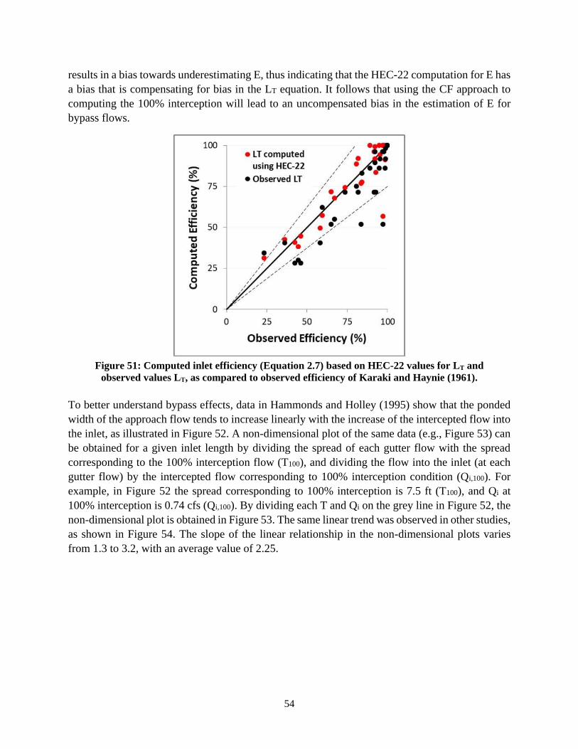
54
results in a bias towards underestimating E, thus indicating that the HEC-22 computation for E has
a bias that is compensating for bias in the LT equation. It follows that using the CF approach to
computing the 100% interception will lead to an uncompensated bias in the estimation of E for
bypass flows.
Figure 51: Computed inlet efficiency (Equation 2.7) based on HEC-22 values for LT and
observed values LT, as compared to observed efficiency of Karaki and Haynie (1961).
To better understand bypass effects, data in Hammonds and Holley (1995) show that the ponded
width of the approach flow tends to increase linearly with the increase of the intercepted flow into
the inlet, as illustrated in Figure 52. A non-dimensional plot of the same data (e.g., Figure 53) can
be obtained for a given inlet length by dividing the spread of each gutter flow with the spread
corresponding to the 100% interception flow (T100), and dividing the flow into the inlet (at each
gutter flow) by the intercepted flow corresponding to 100% interception condition (Qi,100). For
example, in Figure 52 the spread corresponding to 100% interception is 7.5 ft (T100), and Qi at
100% interception is 0.74 cfs (Qi,100). By dividing each T and Qi on the grey line in Figure 52, the
non-dimensional plot is obtained in Figure 53. The same linear trend was observed in other studies,
as shown in Figure 54. The slope of the linear relationship in the non-dimensional plots varies
from 1.3 to 3.2, with an average value of 2.25.
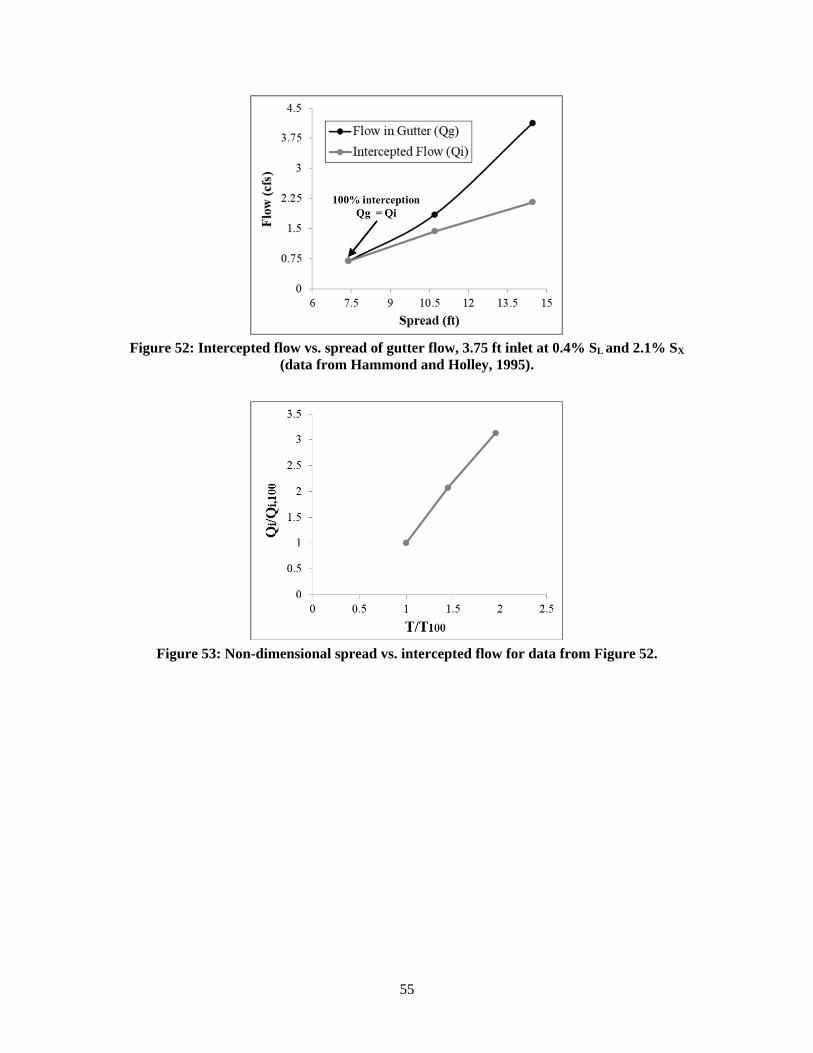
55
Figure 52: Intercepted flow vs. spread of gutter flow, 3.75 ft inlet at 0.4% SL and 2.1% SX
(data from Hammond and Holley, 1995).
Figure 53: Non-dimensional spread vs. intercepted flow for data from Figure 52.
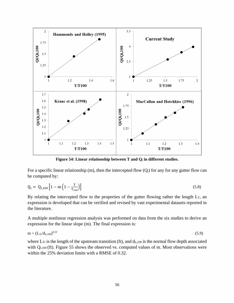
56
Figure 54: Linear relationship between T and Qi in different studies.
For a specific linear relationship (m), then the intercepted flow (Qi) for any for any gutter flow can
be computed by:
Qi = Qi,100 [1 − m (1 −T
T100)] (5.8)
By relating the intercepted flow to the properties of the gutter flowing rather the length LT, an
expression is developed that can be verified and revised by vast experimental datasets reported in
the literature.
A multiple nonlinear regression analysis was performed on data from the six studies to derive an
expression for the linear slope (m). The final expression is:
m = (LTr/dn,100)0.22 (5.9)
where LTr is the length of the upstream transition (ft), and dn,100 is the normal flow depth associated
with Qi,100 (ft). Figure 55 shows the observed vs. computed values of m. Most observations were
within the 25% deviation limits with a RMSE of 0.32.
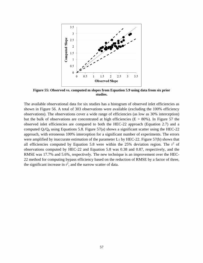
57
Figure 55: Observed vs. computed m slopes from Equation 5.9 using data from six prior
studies.
The available observational data for six studies has a histogram of observed inlet efficiencies as
shown in Figure 56. A total of 303 observations were available (excluding the 100% efficiency
observations). The observations cover a wide range of efficiencies (as low as 30% interception)
but the bulk of observations are concentrated at high efficiencies (E > 80%). In Figure 57 the
observed inlet efficiencies are compared to both the HEC-22 approach (Equation 2.7) and a
computed Qi/Qg using Equations 5.8. Figure 57(a) shows a significant scatter using the HEC-22
approach, with erroneous 100% interception for a significant number of experiments. The errors
were amplified by inaccurate estimation of the parameter LT by HEC-22. Figure 57(b) shows that
all efficiencies computed by Equation 5.8 were within the 25% deviation region. The r2 of
observations computed by HEC-22 and Equation 5.8 was 0.38 and 0.87, respectively, and the
RMSE was 17.7% and 5.6%, respectively. The new technique is an improvement over the HEC-
22 method for computing bypass efficiency based on the reduction of RMSE by a factor of three,
the significant increase in r2, and the narrow scatter of data.
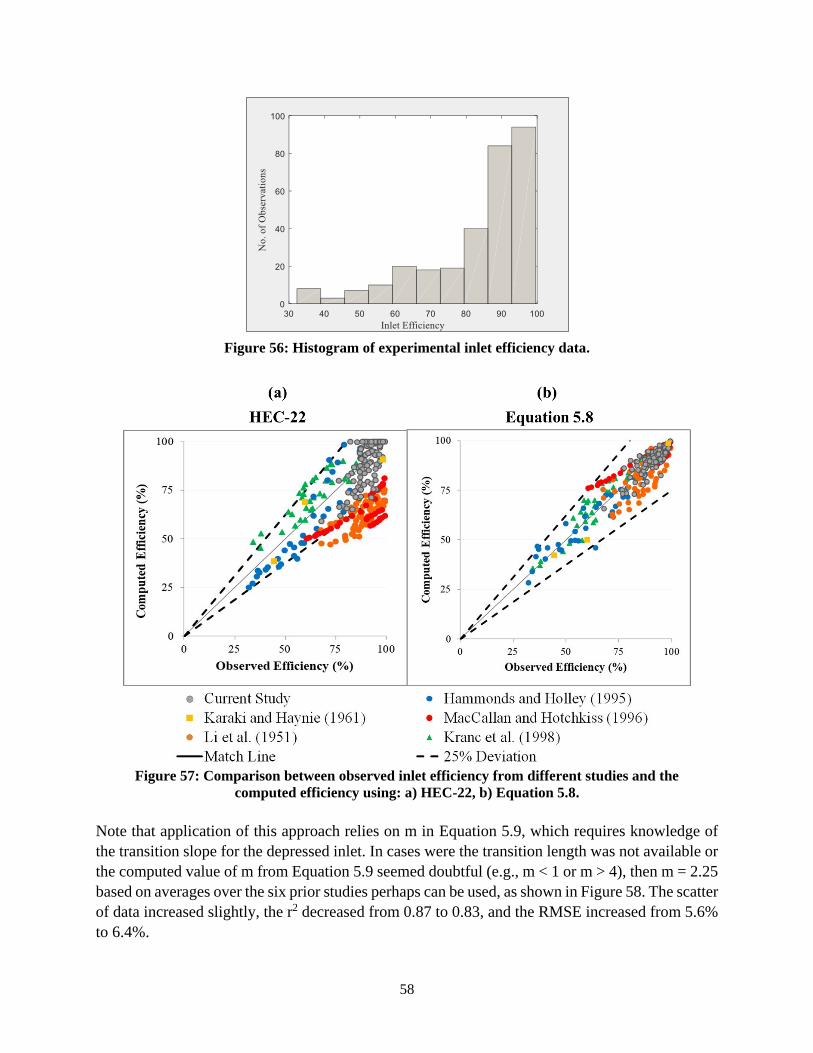
58
Figure 56: Histogram of experimental inlet efficiency data.
Figure 57: Comparison between observed inlet efficiency from different studies and the
computed efficiency using: a) HEC-22, b) Equation 5.8.
Note that application of this approach relies on m in Equation 5.9, which requires knowledge of
the transition slope for the depressed inlet. In cases were the transition length was not available or
the computed value of m from Equation 5.9 seemed doubtful (e.g., m < 1 or m > 4), then m = 2.25
based on averages over the six prior studies perhaps can be used, as shown in Figure 58. The scatter
of data increased slightly, the r2 decreased from 0.87 to 0.83, and the RMSE increased from 5.6%
to 6.4%.
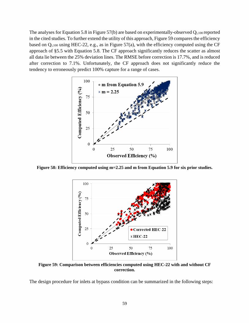
59
The analyses for Equation 5.8 in Figure 57(b) are based on experimentally-observed Qi,100 reported
in the cited studies. To further extend the utility of this approach, Figure 59 compares the efficiency
based on Qi,100 using HEC-22, e.g., as in Figure 57(a), with the efficiency computed using the CF
approach of §5.5 with Equation 5.8. The CF approach significantly reduces the scatter as almost
all data lie between the 25% deviation lines. The RMSE before correction is 17.7%, and is reduced
after correction to 7.1%. Unfortunately, the CF approach does not significantly reduce the
tendency to erroneously predict 100% capture for a range of cases.
Figure 58: Efficiency computed using m=2.25 and m from Equation 5.9 for six prior studies.
Figure 59: Comparison between efficiencies computed using HEC-22 with and without CF
correction.
The design procedure for inlets at bypass condition can be summarized in the following steps:
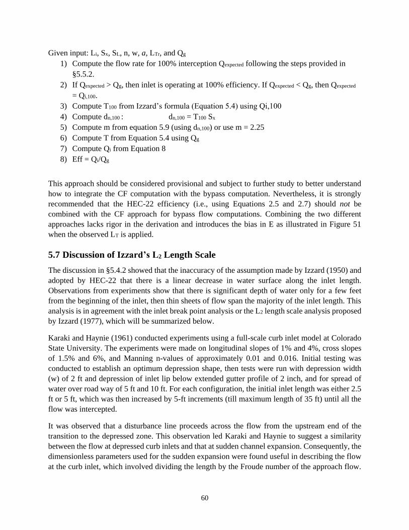
60
Given input: Li, Sx, SL, n, w, a, LTr, and Qg
1) Compute the flow rate for 100% interception Qexpected following the steps provided in
§5.5.2.
2) If Qexpected > Qg, then inlet is operating at 100% efficiency. If Qexpected < Qg, then Qexpected
= Qi,100.
3) Compute T100 from Izzard’s formula (Equation 5.4) using Qi,100
4) Compute dn,100 : dn,100 = T100 Sx
5) Compute m from equation 5.9 (using dn,100) or use m = 2.25
6) Compute T from Equation 5.4 using Qg
7) Compute Qi from Equation 8
8) Eff = Qi/Qg
This approach should be considered provisional and subject to further study to better understand
how to integrate the CF computation with the bypass computation. Nevertheless, it is strongly
recommended that the HEC-22 efficiency (i.e., using Equations 2.5 and 2.7) should not be
combined with the CF approach for bypass flow computations. Combining the two different
approaches lacks rigor in the derivation and introduces the bias in E as illustrated in Figure 51
when the observed LT is applied.
5.7 Discussion of Izzard’s L2 Length Scale
The discussion in §5.4.2 showed that the inaccuracy of the assumption made by Izzard (1950) and
adopted by HEC-22 that there is a linear decrease in water surface along the inlet length.
Observations from experiments show that there is significant depth of water only for a few feet
from the beginning of the inlet, then thin sheets of flow span the majority of the inlet length. This
analysis is in agreement with the inlet break point analysis or the L2 length scale analysis proposed
by Izzard (1977), which will be summarized below.
Karaki and Haynie (1961) conducted experiments using a full-scale curb inlet model at Colorado
State University. The experiments were made on longitudinal slopes of 1% and 4%, cross slopes
of 1.5% and 6%, and Manning n-values of approximately 0.01 and 0.016. Initial testing was
conducted to establish an optimum depression shape, then tests were run with depression width
(w) of 2 ft and depression of inlet lip below extended gutter profile of 2 inch, and for spread of
water over road way of 5 ft and 10 ft. For each configuration, the initial inlet length was either 2.5
ft or 5 ft, which was then increased by 5-ft increments (till maximum length of 35 ft) until all the
flow was intercepted.
It was observed that a disturbance line proceeds across the flow from the upstream end of the
transition to the depressed zone. This observation led Karaki and Haynie to suggest a similarity
between the flow at depressed curb inlets and that at sudden channel expansion. Consequently, the
dimensionless parameters used for the sudden expansion were found useful in describing the flow
at the curb inlet, which involved dividing the length by the Froude number of the approach flow.
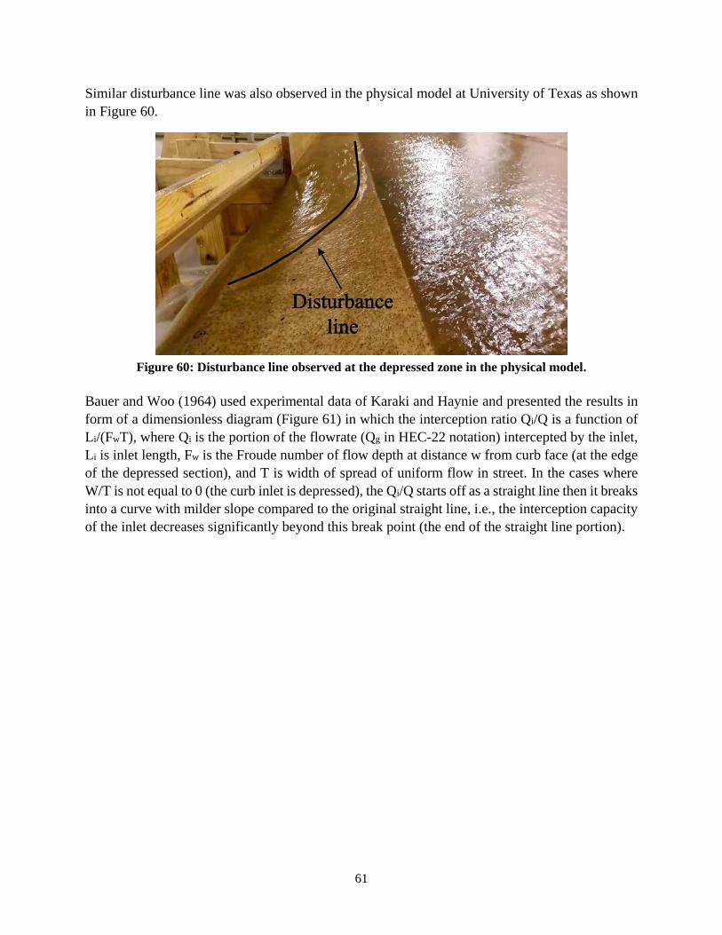
61
Similar disturbance line was also observed in the physical model at University of Texas as shown
in Figure 60.
Figure 60: Disturbance line observed at the depressed zone in the physical model.
Bauer and Woo (1964) used experimental data of Karaki and Haynie and presented the results in
form of a dimensionless diagram (Figure 61) in which the interception ratio Qi/Q is a function of
Li/(FwT), where Qi is the portion of the flowrate (Qg in HEC-22 notation) intercepted by the inlet,
Li is inlet length, Fw is the Froude number of flow depth at distance w from curb face (at the edge
of the depressed section), and T is width of spread of uniform flow in street. In the cases where
W/T is not equal to 0 (the curb inlet is depressed), the Qi/Q starts off as a straight line then it breaks
into a curve with milder slope compared to the original straight line, i.e., the interception capacity
of the inlet decreases significantly beyond this break point (the end of the straight line portion).
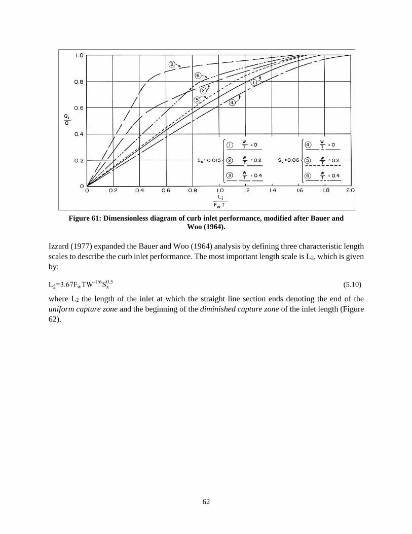
62
Figure 61: Dimensionless diagram of curb inlet performance, modified after Bauer and
Woo (1964).
Izzard (1977) expanded the Bauer and Woo (1964) analysis by defining three characteristic length
scales to describe the curb inlet performance. The most important length scale is L2, which is given
by:
L2=3.67FwTW-1/6Sx0.5 (5.10)
where L2 the length of the inlet at which the straight line section ends denoting the end of the
uniform capture zone and the beginning of the diminished capture zone of the inlet length (Figure
62).
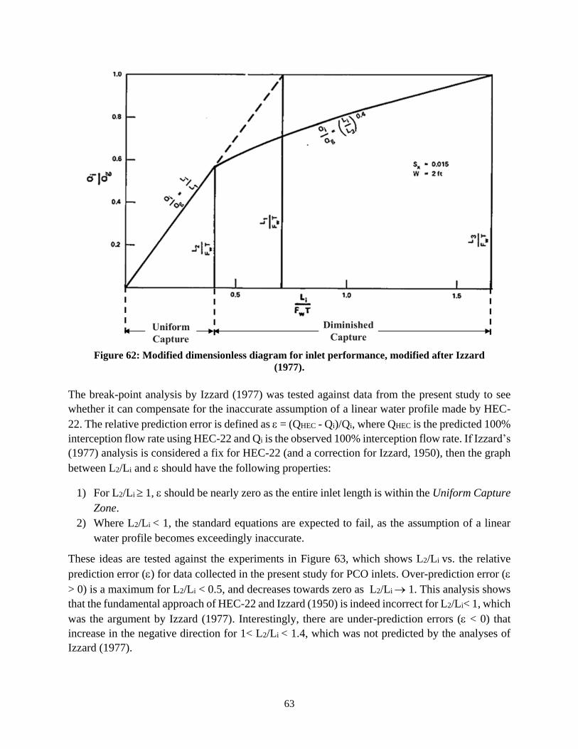
63
Figure 62: Modified dimensionless diagram for inlet performance, modified after Izzard
(1977).
The break-point analysis by Izzard (1977) was tested against data from the present study to see
whether it can compensate for the inaccurate assumption of a linear water profile made by HEC-
22. The relative prediction error is defined as = (QHEC - Qi)/Qi, where QHEC is the predicted 100%
interception flow rate using HEC-22 and Qi is the observed 100% interception flow rate. If Izzard’s
(1977) analysis is considered a fix for HEC-22 (and a correction for Izzard, 1950), then the graph
between L2/Li and should have the following properties:
1) For L2/Li 1, should be nearly zero as the entire inlet length is within the Uniform Capture
Zone.
2) Where L2/Li < 1, the standard equations are expected to fail, as the assumption of a linear
water profile becomes exceedingly inaccurate.
These ideas are tested against the experiments in Figure 63, which shows L2/Li vs. the relative
prediction error () for data collected in the present study for PCO inlets. Over-prediction error (
> 0) is a maximum for L2/Li < 0.5, and decreases towards zero as L2/Li 1. This analysis shows
that the fundamental approach of HEC-22 and Izzard (1950) is indeed incorrect for L2/Li< 1, which
was the argument by Izzard (1977). Interestingly, there are under-prediction errors ( < 0) that
increase in the negative direction for 1< L2/Li < 1.4, which was not predicted by the analyses of
Izzard (1977).
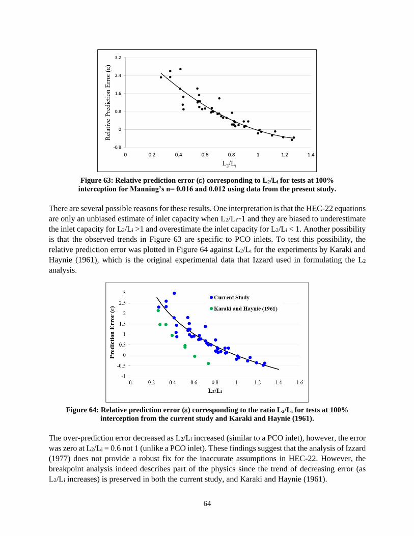
64
Figure 63: Relative prediction error () corresponding to L2/Li for tests at 100%
interception for Manning’s n= 0.016 and 0.012 using data from the present study.
There are several possible reasons for these results. One interpretation is that the HEC-22 equations
are only an unbiased estimate of inlet capacity when L2/Li~1 and they are biased to underestimate
the inlet capacity for L2/Li >1 and overestimate the inlet capacity for L2/Li < 1. Another possibility
is that the observed trends in Figure 63 are specific to PCO inlets. To test this possibility, the
relative prediction error was plotted in Figure 64 against L2/Li for the experiments by Karaki and
Haynie (1961), which is the original experimental data that Izzard used in formulating the L2
analysis.
Figure 64: Relative prediction error () corresponding to the ratio L2/Li for tests at 100%
interception from the current study and Karaki and Haynie (1961).
The over-prediction error decreased as L2/Li increased (similar to a PCO inlet), however, the error
was zero at L2/Li = 0.6 not 1 (unlike a PCO inlet). These findings suggest that the analysis of Izzard
(1977) does not provide a robust fix for the inaccurate assumptions in HEC-22. However, the
breakpoint analysis indeed describes part of the physics since the trend of decreasing error (as
L2/Li increases) is preserved in both the current study, and Karaki and Haynie (1961).

65
An attempt was made to exploit the trend in Figure 63 to develop a correction method for HEC-
22 based on the relationship between L2/Li and the relative predictive error. Given the inlet length
and QHEC, the goal was to apply a correction to HEC-22 so the expected intercepted flow (Qi) could
be obtained. However, applying a correction factor based on L2/Li requires prior knowledge about
Qi for computing L2 (L2 is a function of the Froude number Fw associated with the gutter flow).
Accordingly, this method required a cumbersome iterative solution that produced multiple possible
values for Qi. Eventually, this approach was abandoned for the simpler method described in §5.5.
5.8 Conclusions
HEC-22 provides inaccurate predictions of the 100% interception flow rate for the inlets tested in
this study and other studies, specifically overestimation for the 10 and 15 ft inlets and
underestimation for 5 ft inlets. Three of the main assumptions employed by HEC-22 were
evaluated and potential sources of error were identified. Due to the complexities associated with
some of these inaccurate assumptions, a statistical approach was developed to revise HEC-22 to
avoid introducing complexities that might not be compatible with the scope of experiments in this
study. Experimental data from this study and from five other studies was used to derive a correction
factor for the 100% interception flow rate computed by HEC-22. Applying the correction factor to
HEC-22 produced satisfactory results, reducing the RMSE by a factor of 3.75. A linear relationship
was observed between the spread of gutter flow and the flow intercepted by the inlet. This
relationship was used to develop a new formula for evaluating the efficiency of inlets at bypass
flow condition. The main advantage of this formula is that it is compatible with the typical
experimental procedures in curb inlets studies; therefore the formula could be tested against a large
pool of data from the literature (303 observations) compared to the HEC-22 formula (27
observations). The new formula for bypass flow showed good agreement with the experimental
results, reducing the RMSE from HEC-22 by a factor of three. Finally, the L2 analysis proposed
by Izzard (1977) provides a serious critique to the linear water assumption by HEC-22. Although
Izzard’s analysis was not applied directly to revise HEC-22, it provides an important insight
regarding the higher effectiveness of short inlets compared to longer ones. Finally, changing the
roughness of the model did not have a significant effect on the interception capacity of the 10 ft
inlet, possibly due to the increase in the capacity of the depressed gutter associated with a smoother
surface.
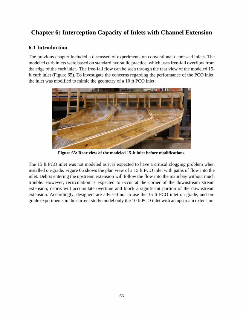
66
Chapter 6: Interception Capacity of Inlets with Channel Extension
6.1 Introduction
The previous chapter included a discussed of experiments on conventional depressed inlets. The
modeled curb inlets were based on standard hydraulic practice, which uses free-fall overflow from
the edge of the curb inlet. The free-fall flow can be seen through the rear view of the modeled 15-
ft curb inlet (Figure 65). To investigate the concerns regarding the performance of the PCO inlet,
the inlet was modified to mimic the geometry of a 10 ft PCO inlet.
Figure 65: Rear view of the modeled 15-ft inlet before modifications.
The 15 ft PCO inlet was not modeled as it is expected to have a critical clogging problem when
installed on-grade. Figure 66 shows the plan view of a 15 ft PCO inlet with paths of flow into the
inlet. Debris entering the upstream extension will follow the flow into the main bay without much
trouble. However, recirculation is expected to occur at the corner of the downstream stream
extension; debris will accumulate overtime and block a significant portion of the downstream
extension. Accordingly, designers are advised not to use the 15 ft PCO inlet on-grade, and on-
grade experiments in the current study model only the 10 ft PCO inlet with an upstream extension.
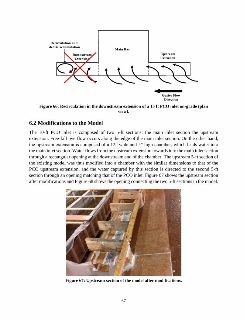
67
Figure 66: Recirculation in the downstream extension of a 15 ft PCO inlet on-grade (plan
view).
6.2 Modifications to the Model
The 10-ft PCO inlet is composed of two 5-ft sections: the main inlet section the upstream
extension. Free-fall overflow occurs along the edge of the main inlet section. On the other hand,
the upstream extension is composed of a 12” wide and 5” high chamber, which leads water into
the main inlet section. Water flows from the upstream extension towards into the main inlet section
through a rectangular opening at the downstream end of the chamber. The upstream 5-ft section of
the existing model was thus modified into a chamber with the similar dimensions to that of the
PCO upstream extension, and the water captured by this section is directed to the second 5-ft
section through an opening matching that of the PCO inlet. Figure 67 shows the upstream section
after modifications and Figure 68 shows the opening connecting the two 5-ft sections in the model.
Figure 67: Upstream section of the model after modifications.
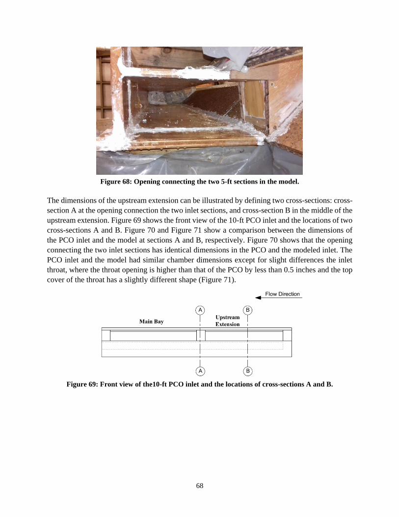
68
Figure 68: Opening connecting the two 5-ft sections in the model.
The dimensions of the upstream extension can be illustrated by defining two cross-sections: cross-
section A at the opening connection the two inlet sections, and cross-section B in the middle of the
upstream extension. Figure 69 shows the front view of the 10-ft PCO inlet and the locations of two
cross-sections A and B. Figure 70 and Figure 71 show a comparison between the dimensions of
the PCO inlet and the model at sections A and B, respectively. Figure 70 shows that the opening
connecting the two inlet sections has identical dimensions in the PCO and the modeled inlet. The
PCO inlet and the model had similar chamber dimensions except for slight differences the inlet
throat, where the throat opening is higher than that of the PCO by less than 0.5 inches and the top
cover of the throat has a slightly different shape (Figure 71).
Figure 69: Front view of the10-ft PCO inlet and the locations of cross-sections A and B.
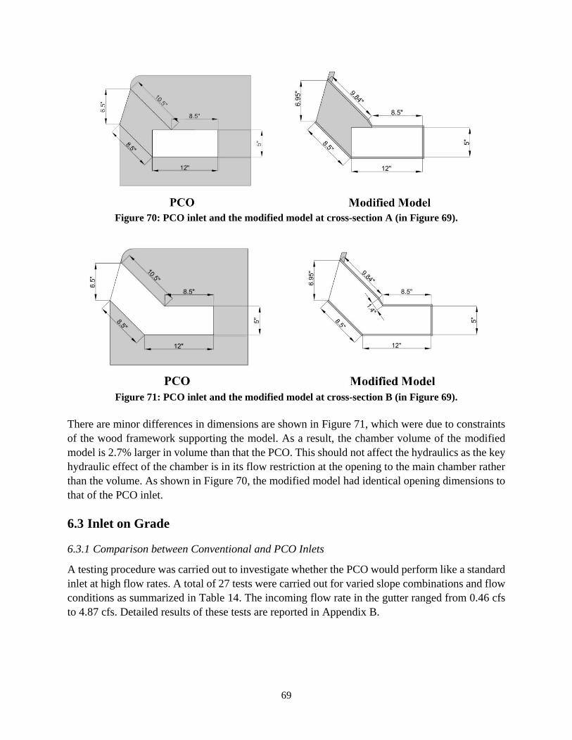
69
Figure 70: PCO inlet and the modified model at cross-section A (in Figure 69).
Figure 71: PCO inlet and the modified model at cross-section B (in Figure 69).
There are minor differences in dimensions are shown in Figure 71, which were due to constraints
of the wood framework supporting the model. As a result, the chamber volume of the modified
model is 2.7% larger in volume than that the PCO. This should not affect the hydraulics as the key
hydraulic effect of the chamber is in its flow restriction at the opening to the main chamber rather
than the volume. As shown in Figure 70, the modified model had identical opening dimensions to
that of the PCO inlet.
6.3 Inlet on Grade
6.3.1 Comparison between Conventional and PCO Inlets
A testing procedure was carried out to investigate whether the PCO would perform like a standard
inlet at high flow rates. A total of 27 tests were carried out for varied slope combinations and flow
conditions as summarized in Table 14. The incoming flow rate in the gutter ranged from 0.46 cfs
to 4.87 cfs. Detailed results of these tests are reported in Appendix B.
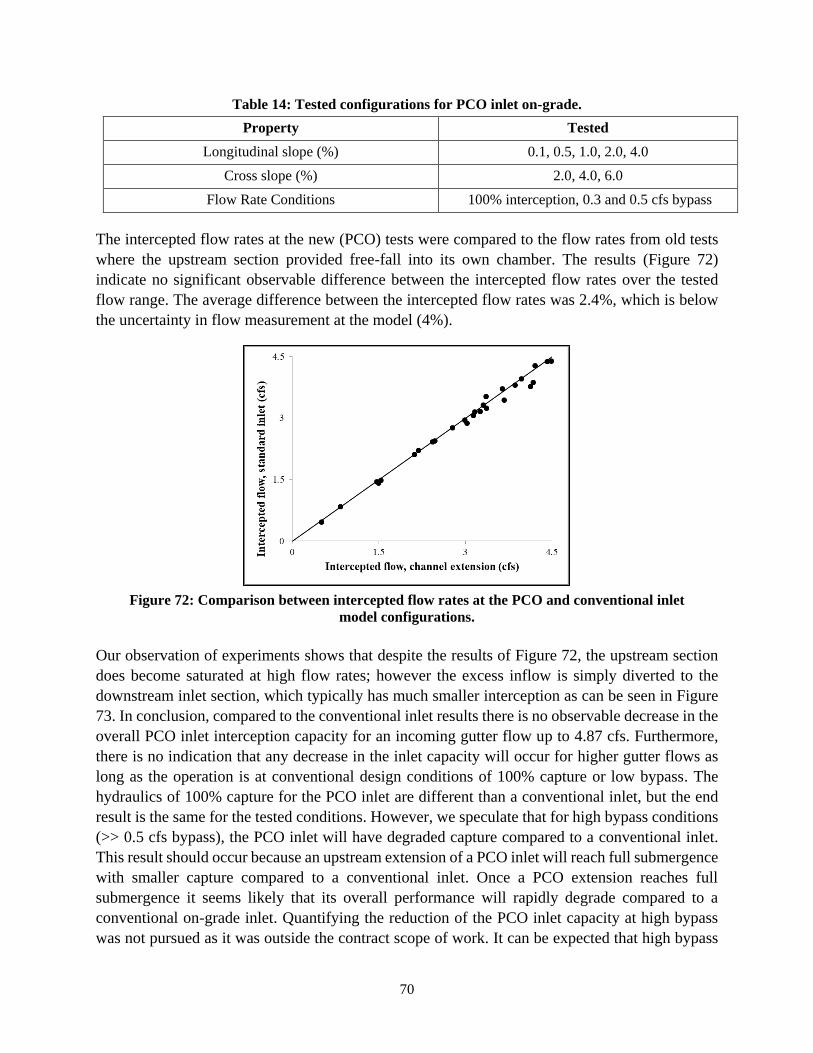
70
Table 14: Tested configurations for PCO inlet on-grade.
Property Tested
Longitudinal slope (%) 0.1, 0.5, 1.0, 2.0, 4.0
Cross slope (%) 2.0, 4.0, 6.0
Flow Rate Conditions 100% interception, 0.3 and 0.5 cfs bypass
The intercepted flow rates at the new (PCO) tests were compared to the flow rates from old tests
where the upstream section provided free-fall into its own chamber. The results (Figure 72)
indicate no significant observable difference between the intercepted flow rates over the tested
flow range. The average difference between the intercepted flow rates was 2.4%, which is below
the uncertainty in flow measurement at the model (4%).
Figure 72: Comparison between intercepted flow rates at the PCO and conventional inlet
model configurations.
Our observation of experiments shows that despite the results of Figure 72, the upstream section
does become saturated at high flow rates; however the excess inflow is simply diverted to the
downstream inlet section, which typically has much smaller interception as can be seen in Figure
73. In conclusion, compared to the conventional inlet results there is no observable decrease in the
overall PCO inlet interception capacity for an incoming gutter flow up to 4.87 cfs. Furthermore,
there is no indication that any decrease in the inlet capacity will occur for higher gutter flows as
long as the operation is at conventional design conditions of 100% capture or low bypass. The
hydraulics of 100% capture for the PCO inlet are different than a conventional inlet, but the end
result is the same for the tested conditions. However, we speculate that for high bypass conditions
(>> 0.5 cfs bypass), the PCO inlet will have degraded capture compared to a conventional inlet.
This result should occur because an upstream extension of a PCO inlet will reach full submergence
with smaller capture compared to a conventional inlet. Once a PCO extension reaches full
submergence it seems likely that its overall performance will rapidly degrade compared to a
conventional on-grade inlet. Quantifying the reduction of the PCO inlet capacity at high bypass
was not pursued as it was outside the contract scope of work. It can be expected that high bypass
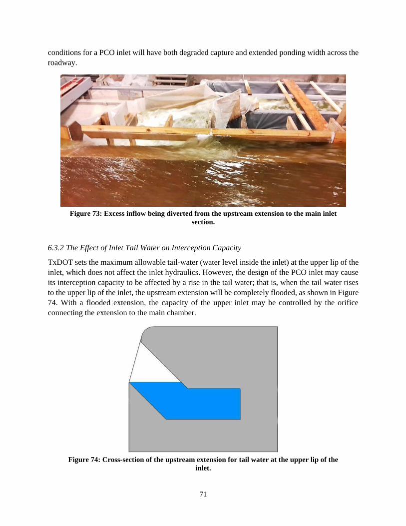
71
conditions for a PCO inlet will have both degraded capture and extended ponding width across the
roadway.
Figure 73: Excess inflow being diverted from the upstream extension to the main inlet
section.
6.3.2 The Effect of Inlet Tail Water on Interception Capacity
TxDOT sets the maximum allowable tail-water (water level inside the inlet) at the upper lip of the
inlet, which does not affect the inlet hydraulics. However, the design of the PCO inlet may cause
its interception capacity to be affected by a rise in the tail water; that is, when the tail water rises
to the upper lip of the inlet, the upstream extension will be completely flooded, as shown in Figure
74. With a flooded extension, the capacity of the upper inlet may be controlled by the orifice
connecting the extension to the main chamber.
Figure 74: Cross-section of the upstream extension for tail water at the upper lip of the
inlet.
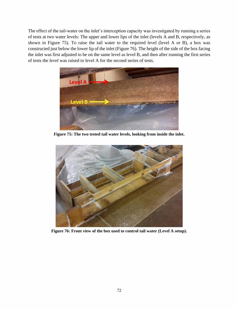
72
The effect of the tail-water on the inlet’s interception capacity was investigated by running a series
of tests at two water levels: The upper and lower lips of the inlet (levels A and B, respectively, as
shown in Figure 75). To raise the tail water to the required level (level A or B), a box was
constructed just below the lower lip of the inlet (Figure 76). The height of the side of the box facing
the inlet was first adjusted to be on the same level as level B, and then after running the first series
of tests the level was raised to level A for the second series of tests.
Figure 75: The two tested tail water levels, looking from inside the inlet.
Figure 76: Front view of the box used to control tail water (Level A setup).
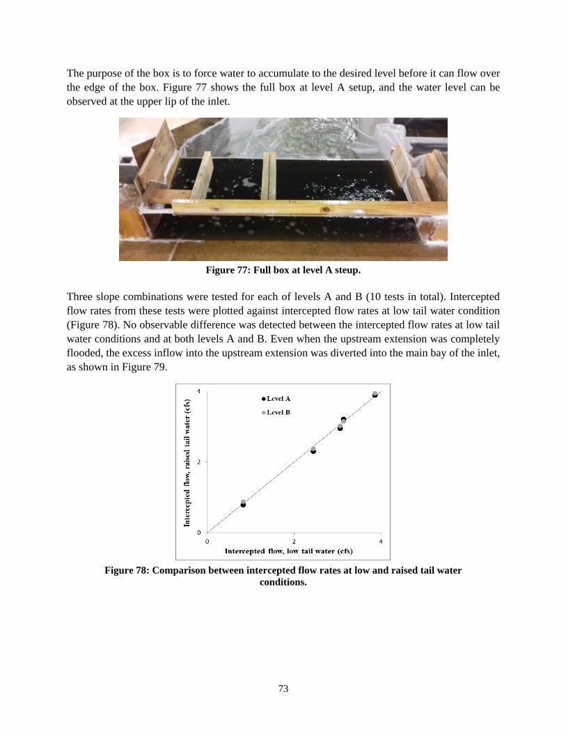
73
The purpose of the box is to force water to accumulate to the desired level before it can flow over
the edge of the box. Figure 77 shows the full box at level A setup, and the water level can be
observed at the upper lip of the inlet.
Figure 77: Full box at level A steup.
Three slope combinations were tested for each of levels A and B (10 tests in total). Intercepted
flow rates from these tests were plotted against intercepted flow rates at low tail water condition
(Figure 78). No observable difference was detected between the intercepted flow rates at low tail
water conditions and at both levels A and B. Even when the upstream extension was completely
flooded, the excess inflow into the upstream extension was diverted into the main bay of the inlet,
as shown in Figure 79.
Figure 78: Comparison between intercepted flow rates at low and raised tail water
conditions.
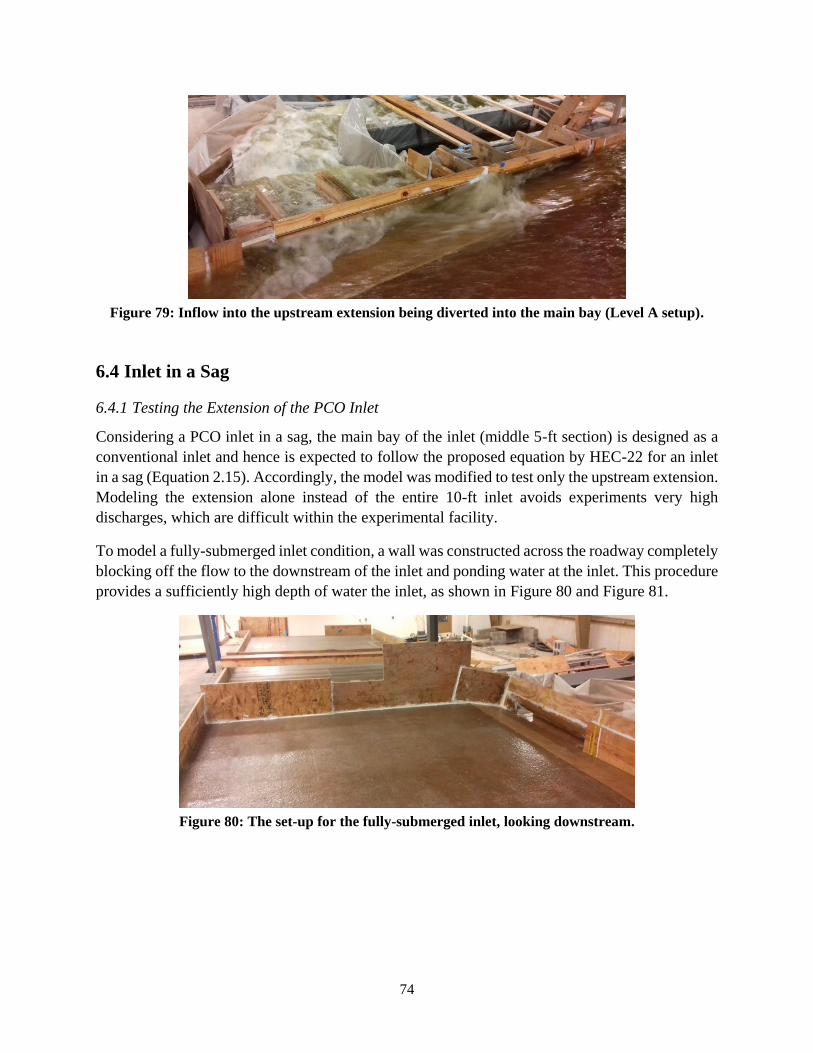
74
Figure 79: Inflow into the upstream extension being diverted into the main bay (Level A setup).
6.4 Inlet in a Sag
6.4.1 Testing the Extension of the PCO Inlet
Considering a PCO inlet in a sag, the main bay of the inlet (middle 5-ft section) is designed as a
conventional inlet and hence is expected to follow the proposed equation by HEC-22 for an inlet
in a sag (Equation 2.15). Accordingly, the model was modified to test only the upstream extension.
Modeling the extension alone instead of the entire 10-ft inlet avoids experiments very high
discharges, which are difficult within the experimental facility.
To model a fully-submerged inlet condition, a wall was constructed across the roadway completely
blocking off the flow to the downstream of the inlet and ponding water at the inlet. This procedure
provides a sufficiently high depth of water the inlet, as shown in Figure 80 and Figure 81.
Figure 80: The set-up for the fully-submerged inlet, looking downstream.
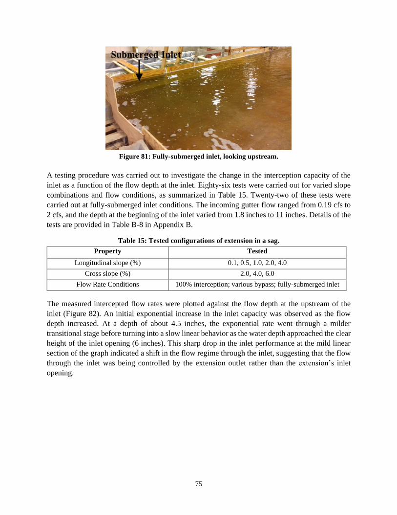
75
Figure 81: Fully-submerged inlet, looking upstream.
A testing procedure was carried out to investigate the change in the interception capacity of the
inlet as a function of the flow depth at the inlet. Eighty-six tests were carried out for varied slope
combinations and flow conditions, as summarized in Table 15. Twenty-two of these tests were
carried out at fully-submerged inlet conditions. The incoming gutter flow ranged from 0.19 cfs to
2 cfs, and the depth at the beginning of the inlet varied from 1.8 inches to 11 inches. Details of the
tests are provided in Table B-8 in Appendix B.
Table 15: Tested configurations of extension in a sag.
Property Tested
Longitudinal slope (%) 0.1, 0.5, 1.0, 2.0, 4.0
Cross slope (%) 2.0, 4.0, 6.0
Flow Rate Conditions 100% interception; various bypass; fully-submerged inlet
The measured intercepted flow rates were plotted against the flow depth at the upstream of the
inlet (Figure 82). An initial exponential increase in the inlet capacity was observed as the flow
depth increased. At a depth of about 4.5 inches, the exponential rate went through a milder
transitional stage before turning into a slow linear behavior as the water depth approached the clear
height of the inlet opening (6 inches). This sharp drop in the inlet performance at the mild linear
section of the graph indicated a shift in the flow regime through the inlet, suggesting that the flow
through the inlet was being controlled by the extension outlet rather than the extension’s inlet
opening.
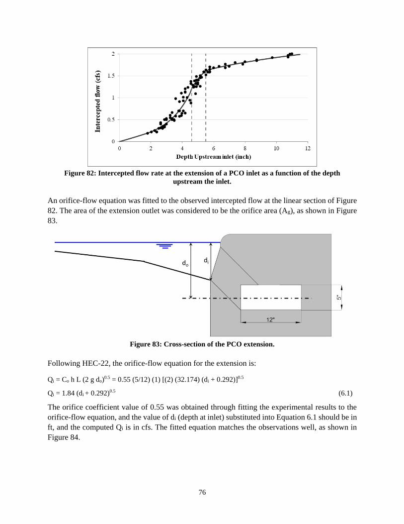
76
Figure 82: Intercepted flow rate at the extension of a PCO inlet as a function of the depth
upstream the inlet.
An orifice-flow equation was fitted to the observed intercepted flow at the linear section of Figure
82. The area of the extension outlet was considered to be the orifice area (Ag), as shown in Figure
83.
Figure 83: Cross-section of the PCO extension.
Following HEC-22, the orifice-flow equation for the extension is:
Qi = Co h L (2 g do)0.5 = 0.55 (5/12) (1) [(2) (32.174) (di + 0.292)]0.5
Qi = 1.84 (di + 0.292)0.5 (6.1)
The orifice coefficient value of 0.55 was obtained through fitting the experimental results to the
orifice-flow equation, and the value of di (depth at inlet) substituted into Equation 6.1 should be in
ft, and the computed Qi is in cfs. The fitted equation matches the observations well, as shown in
Figure 84.
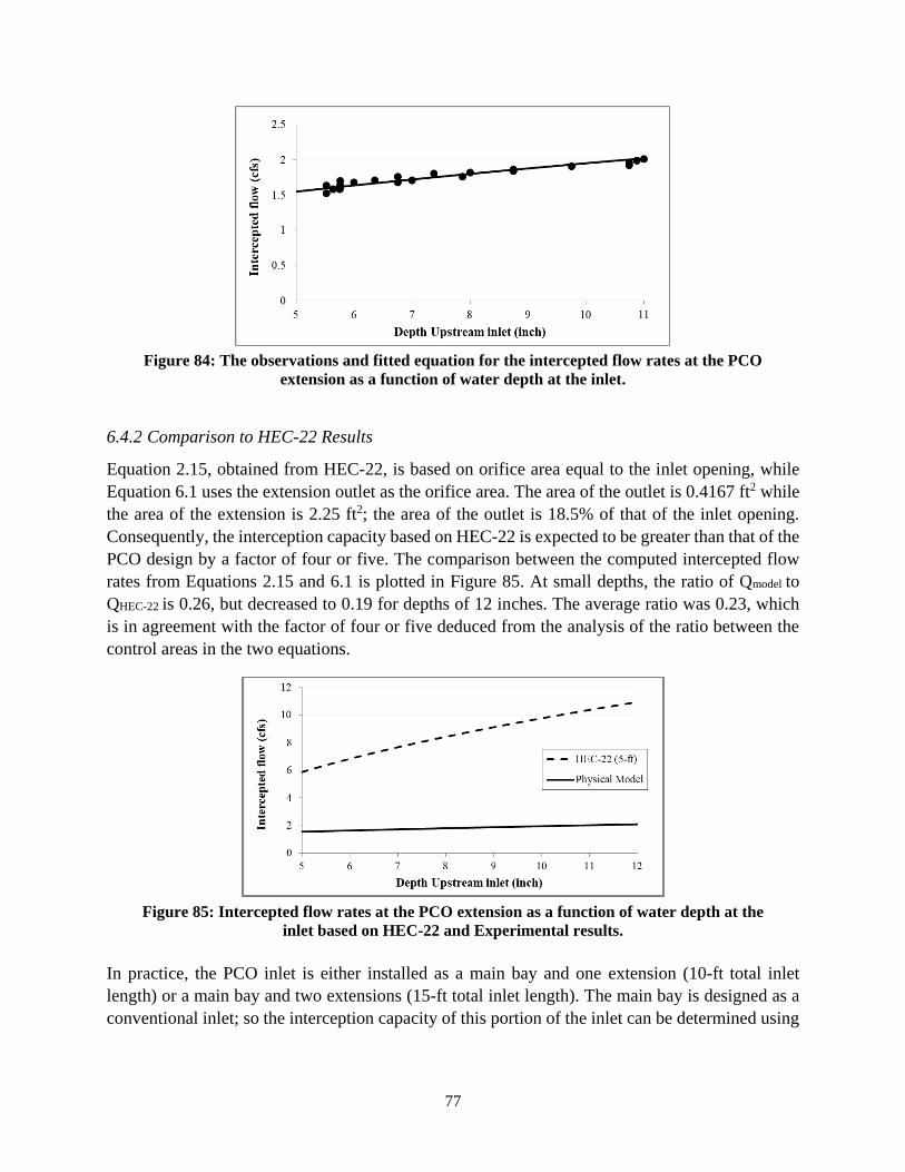
77
Figure 84: The observations and fitted equation for the intercepted flow rates at the PCO
extension as a function of water depth at the inlet.
6.4.2 Comparison to HEC-22 Results
Equation 2.15, obtained from HEC-22, is based on orifice area equal to the inlet opening, while
Equation 6.1 uses the extension outlet as the orifice area. The area of the outlet is 0.4167 ft2 while
the area of the extension is 2.25 ft2; the area of the outlet is 18.5% of that of the inlet opening.
Consequently, the interception capacity based on HEC-22 is expected to be greater than that of the
PCO design by a factor of four or five. The comparison between the computed intercepted flow
rates from Equations 2.15 and 6.1 is plotted in Figure 85. At small depths, the ratio of Qmodel to
QHEC-22 is 0.26, but decreased to 0.19 for depths of 12 inches. The average ratio was 0.23, which
is in agreement with the factor of four or five deduced from the analysis of the ratio between the
control areas in the two equations.
Figure 85: Intercepted flow rates at the PCO extension as a function of water depth at the
inlet based on HEC-22 and Experimental results.
In practice, the PCO inlet is either installed as a main bay and one extension (10-ft total inlet
length) or a main bay and two extensions (15-ft total inlet length). The main bay is designed as a
conventional inlet; so the interception capacity of this portion of the inlet can be determined using
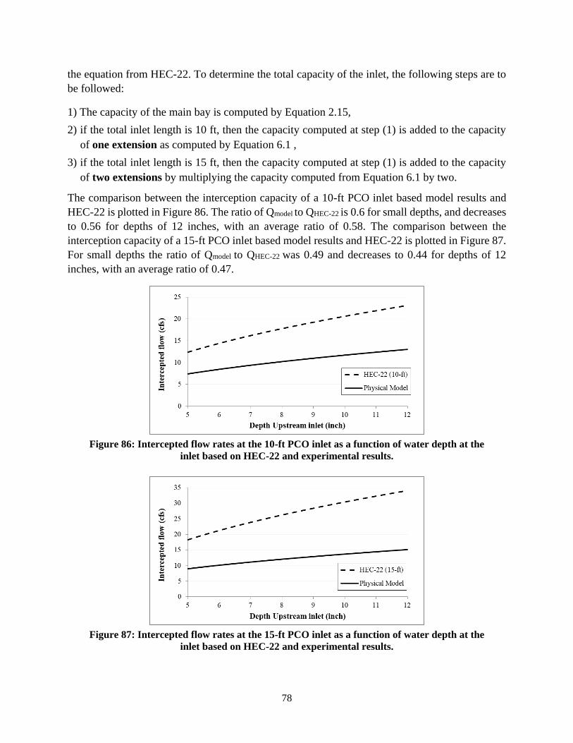
78
the equation from HEC-22. To determine the total capacity of the inlet, the following steps are to
be followed:
1) The capacity of the main bay is computed by Equation 2.15,
2) if the total inlet length is 10 ft, then the capacity computed at step (1) is added to the capacity
of one extension as computed by Equation 6.1 ,
3) if the total inlet length is 15 ft, then the capacity computed at step (1) is added to the capacity
of two extensions by multiplying the capacity computed from Equation 6.1 by two.
The comparison between the interception capacity of a 10-ft PCO inlet based model results and
HEC-22 is plotted in Figure 86. The ratio of Qmodel to QHEC-22 is 0.6 for small depths, and decreases
to 0.56 for depths of 12 inches, with an average ratio of 0.58. The comparison between the
interception capacity of a 15-ft PCO inlet based model results and HEC-22 is plotted in Figure 87.
For small depths the ratio of Qmodel to QHEC-22 was 0.49 and decreases to 0.44 for depths of 12
inches, with an average ratio of 0.47.
Figure 86: Intercepted flow rates at the 10-ft PCO inlet as a function of water depth at the
inlet based on HEC-22 and experimental results.
Figure 87: Intercepted flow rates at the 15-ft PCO inlet as a function of water depth at the
inlet based on HEC-22 and experimental results.
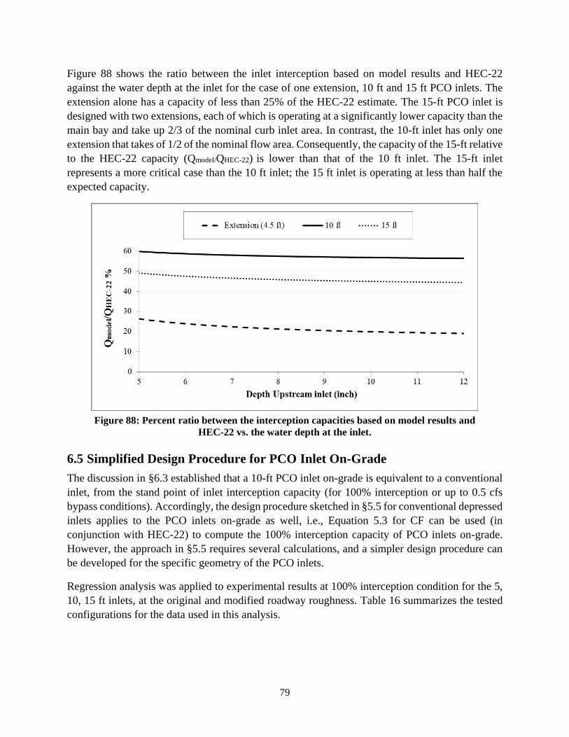
79
Figure 88 shows the ratio between the inlet interception based on model results and HEC-22
against the water depth at the inlet for the case of one extension, 10 ft and 15 ft PCO inlets. The
extension alone has a capacity of less than 25% of the HEC-22 estimate. The 15-ft PCO inlet is
designed with two extensions, each of which is operating at a significantly lower capacity than the
main bay and take up 2/3 of the nominal curb inlet area. In contrast, the 10-ft inlet has only one
extension that takes of 1/2 of the nominal flow area. Consequently, the capacity of the 15-ft relative
to the HEC-22 capacity (Qmodel/QHEC-22) is lower than that of the 10 ft inlet. The 15-ft inlet
represents a more critical case than the 10 ft inlet; the 15 ft inlet is operating at less than half the
expected capacity.
Figure 88: Percent ratio between the interception capacities based on model results and
HEC-22 vs. the water depth at the inlet.
6.5 Simplified Design Procedure for PCO Inlet On-Grade
The discussion in §6.3 established that a 10-ft PCO inlet on-grade is equivalent to a conventional
inlet, from the stand point of inlet interception capacity (for 100% interception or up to 0.5 cfs
bypass conditions). Accordingly, the design procedure sketched in §5.5 for conventional depressed
inlets applies to the PCO inlets on-grade as well, i.e., Equation 5.3 for CF can be used (in
conjunction with HEC-22) to compute the 100% interception capacity of PCO inlets on-grade.
However, the approach in §5.5 requires several calculations, and a simpler design procedure can
be developed for the specific geometry of the PCO inlets.
Regression analysis was applied to experimental results at 100% interception condition for the 5,
10, 15 ft inlets, at the original and modified roadway roughness. Table 16 summarizes the tested
configurations for the data used in this analysis.
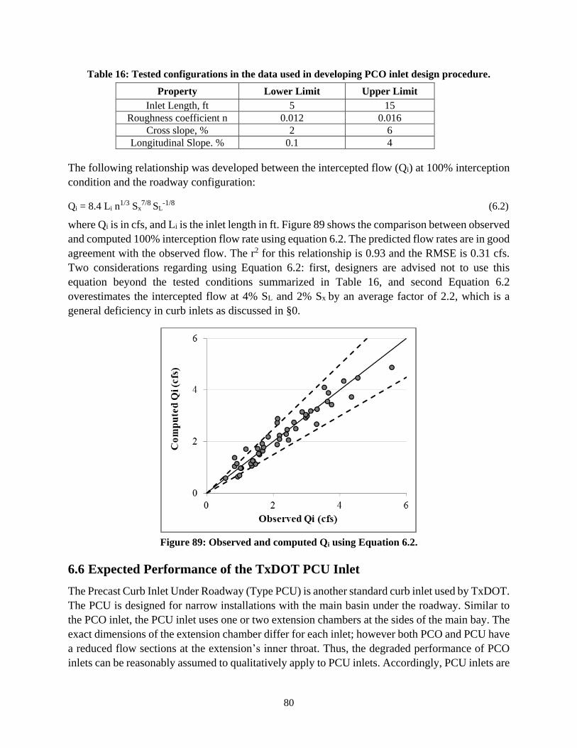
80
Table 16: Tested configurations in the data used in developing PCO inlet design procedure.
Property Lower Limit Upper Limit
Inlet Length, ft 5 15
Roughness coefficient n 0.012 0.016
Cross slope, % 2 6
Longitudinal Slope. % 0.1 4
The following relationship was developed between the intercepted flow (Qi) at 100% interception
condition and the roadway configuration:
Qi = 8.4 Li n1/3 Sx
7/8 SL-1/8 (6.2)
where Qi is in cfs, and Li is the inlet length in ft. Figure 89 shows the comparison between observed
and computed 100% interception flow rate using equation 6.2. The predicted flow rates are in good
agreement with the observed flow. The r2 for this relationship is 0.93 and the RMSE is 0.31 cfs.
Two considerations regarding using Equation 6.2: first, designers are advised not to use this
equation beyond the tested conditions summarized in Table 16, and second Equation 6.2
overestimates the intercepted flow at 4% SL and 2% Sx by an average factor of 2.2, which is a
general deficiency in curb inlets as discussed in §0.
Figure 89: Observed and computed Qi using Equation 6.2.
6.6 Expected Performance of the TxDOT PCU Inlet
The Precast Curb Inlet Under Roadway (Type PCU) is another standard curb inlet used by TxDOT.
The PCU is designed for narrow installations with the main basin under the roadway. Similar to
the PCO inlet, the PCU inlet uses one or two extension chambers at the sides of the main bay. The
exact dimensions of the extension chamber differ for each inlet; however both PCO and PCU have
a reduced flow sections at the extension’s inner throat. Thus, the degraded performance of PCO
inlets can be reasonably assumed to qualitatively apply to PCU inlets. Accordingly, PCU inlets are

81
expected to have a similar performance to a standard inlet for an on-grade configuration (under
100% interception or low bypass-flow conditions), and reduced capture when installed in a sag.
However, the throat area of the PCU extension is about 11% larger than that of a PCO extension,
so the capacity of a PCU inlet in a sag is expected to be somewhat higher than the tested PCO
configuration. It seems unlikely that this small increase in the throat area would be enough for the
PCU to achieve the same capture as a standard inlet in a sag, but establishment of a quantitative
value for the reduced capture of the PCU in a sag requires either direct testing of a PCU
configuration or development of adequate hydraulics theory that explains the PCO reduction and
is extensible to the PCU.
6.7 Conclusions
A series of tests was conducted to investigate the effect of the constricted upstream extension on
the overall interception capacity of the inlet. Results from these tests showed no notable difference
from interception capacity of a 10-ft inlet with a free-fall overflow along the entire inlet length.
However, degraded inlet capture is expected at higher bypass flow conditions (Qbypass >> 0.5 cfs).
Another series of tests showed that a tail water as high as the upper lip of the inlet (maximum
allowable level by TxDOT) will not affect the inlet’s interception capacity. Interestingly, the
observed inlet capacities are very robust to the significant changes in the hydraulic configurations
between the PCO and non-PCO inlets. Although the constriction of the upstream inlet did not
cause further limitation of the inlet’s interception capacity, it must be emphasized that the HEC-
22 design equations cannot be directly applied to the PCO inlet under all conditions, as discussed
in §5.4.
The capacity of the extension of the PCO inlet in a sag was investigated through a series of
experiments. Results from these experiments showed that HEC-22 significantly overestimates the
interception capacity of the extension. The design of the extension changes the orifice control-
section from the inlet opening to the smaller opening of the inner outlet of the extension. An
equation was proposed for the capacity of the extension as a function of the depth at the inlet. This
equation was used in combination with HEC-22 to determine the capacity of the 10 ft and 15 ft
PCO inlets. This analysis showed that the capacity of the 10 ft and the 15-ft PCO inlet are about
58% and 47% of the capacities computed using the HEC-22 equation. The significant decrease in
the interception capacity of the PCO inlet calls for careful consideration from designers upon
deciding to install these inlets in a sag, particularly for a 15-ft PCO inlet
82
Chapter 7: Conclusions
7.1 Summary
The objective of this study is to provide updated design guidance on the TxDOT PCO inlet. This
objective involved studying the effects of flush slab support on the inlet capacity, the performance
of conventional depressed inlets, and the potential flow restrictions in inlets with channel
extensions. A full-scale physical model of a depressed inlet mounted on a roadway with adjustable
slopes was used to address these issues. A comparison between full-scale and scaled models of
depressed and undepressed inlets in South Africa showed a significant mismatch between the two
cases, especially at shallow water depth for depressed inlets. Therefore, the use of a full-scale
model eliminated potential sources of error due to misrepresentation of Reynolds number effects
in scaled models. Experimental data from this study and the literature were employed in assessing
the design procedures in HEC-22 and proposing revisions to HEC-22. Conclusions and
recommendations from this study are summarized in Table 17.
7.2 Slab Supports
A review of 22 studies from 1950 to 2012 did not produce any evidence in support of the statement
by HEC-22 that flush slab supports decrease the effectiveness of the inlet by as much as 50%. Full-
scale experiments on 10 and 15 ft inlets with and without slab supports showed no observable
difference in the intercepted flow rate in the two cases. The hydraulic effects of the slab support
are local and do not interfere with the ponded width or the intercepted flow. Thus, the presence of
small slab supports should be ignored in hydraulic computations and the total inlet length should
be computed from the inlet opening to the inlet end without any adjustment for slab supports.
However, the HEC-22 statement that slab supports have a significant effect on inlet clogging is
not contradicted by the present work and potential for clogging should be considered in any design.
We can also speculate that clogging will be worse for PCO and PCU inlets due to the reduced
throat area at the extensions. Analysis of clogging effects was beyond the scope of the present
study.
7.3 Depressed Curb Inlets
The 5, 10, and 15 ft inlets were tests at the original model roughness, and the 10 ft inlet was tested
at a smoother roadway roughness. On comparing the tests for 10 ft inlets at different roadway
roughness, only a minor decrease in inlet interception capacity was observed. The intercepted flow
rates at 100% interception condition for the 5, 10, and 15 ft inlets were compared to predictions
by HEC-22. This comparison showed that HEC-22 overestimated the intercepted flow by the 10
and 15 ft inlets, and underestimated the capacity of 5 ft inlets. Potential sources of errors in the
assumptions employed by HEC-22 include: 1) the invalid assumption of linear decrease in water
surface profile along the length of the inlet, 2) oversimplification of flow immediately upstream
the inlet that led to discrepancies between the observed and computed capacity of the depressed
gutter section, and 3) using the equivalent slope Se to account for the combined effects of the two
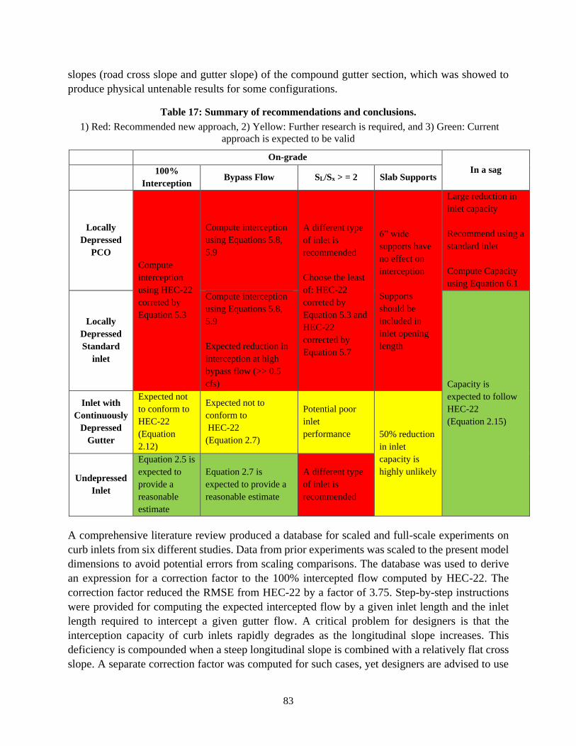
83
slopes (road cross slope and gutter slope) of the compound gutter section, which was showed to
produce physical untenable results for some configurations.
Table 17: Summary of recommendations and conclusions.
1) Red: Recommended new approach, 2) Yellow: Further research is required, and 3) Green: Current
approach is expected to be valid
On-grade
In a sag
100%
Interception Bypass Flow SL/Sx > = 2 Slab Supports
Locally
Depressed
PCO
Compute
interception
using HEC-22
correted by
Equation 5.3
Compute interception
using Equations 5.8,
5.9
A different type
of inlet is
recommended
Choose the least
of: HEC-22
correted by
Equation 5.3 and
HEC-22
corrected by
Equation 5.7
6” wide
supports have
no effect on
interception
Supports
should be
included in
inlet opening
length
Large reduction in
inlet capacity
Recommend using a
standard inlet
Compute Capacity
using Equation 6.1
Locally
Depressed
Standard
inlet
Compute interception
using Equations 5.8,
5.9
Expected reduction in
interception at high
bypass flow (>> 0.5
cfs) Capacity is
expected to follow
HEC-22
(Equation 2.15)
Inlet with
Continuously
Depressed
Gutter
Expected not
to conform to
HEC-22
(Equation
2.12)
Expected not to
conform to
HEC-22
(Equation 2.7)
Potential poor
inlet
performance 50% reduction
in inlet
capacity is
highly unlikely Undepressed
Inlet
Equation 2.5 is
expected to
provide a
reasonable
estimate
Equation 2.7 is
expected to provide a
reasonable estimate
A different type
of inlet is
recommended
A comprehensive literature review produced a database for scaled and full-scale experiments on
curb inlets from six different studies. Data from prior experiments was scaled to the present model
dimensions to avoid potential errors from scaling comparisons. The database was used to derive
an expression for a correction factor to the 100% intercepted flow computed by HEC-22. The
correction factor reduced the RMSE from HEC-22 by a factor of 3.75. Step-by-step instructions
were provided for computing the expected intercepted flow by a given inlet length and the inlet
length required to intercept a given gutter flow. A critical problem for designers is that the
interception capacity of curb inlets rapidly degrades as the longitudinal slope increases. This
deficiency is compounded when a steep longitudinal slope is combined with a relatively flat cross
slope. A separate correction factor was computed for such cases, yet designers are advised to use

84
a different type of inlet (e.g. grate or combination inlet) when the ratio of SL/Sx is greater than or
equal to two.
During analysis of data for inlets at bypass condition (less than 100% efficiency), a linear
relationship was observed between the intercepted flow rate (Qi) and the spread of the gutter flow
(T). The proposed formula by HEC-22 for bypass flow is based on the parameter LT, the required
inlet length for 100% capture of the approaching gutter flow. Experimental data for this parameter
is scarce in the literature due to the practical difficulties of setting up experiments with variable
inlet length. Proposing a formula based on Qi and T allows for using vast experimental datasets
reported in the literature. The new formula was tested against 303 observations from six different
studies, and showed good agreement with these observations. The RMSE was reduced by a factor
of three compared to the HEC-22 approach.
Izzard (1977) argued that after a certain point along the inlet length (L2), the intercepted flow by
the inlet decreases drastically. His argument challenges the assumption of a linearly decreases
water profile along the inlet length, which is common in HEC-22 equations and other design
approaches. Analysis of the relationship between the error in HEC-22 predictions and the L2 length
scale showed that HEC-22 only accurately predicts the interception capacity of a PCO inlet of
length Li equal to L2, which is support’s Izzard’s argument. However, this finding was not
replicable with data from another study, which suggests that Izzard’s analysis does not provide a
robust fix for the inaccurate assumptions in HEC-22. The main insight gained from Izzard’s
analysis is that shorter inlets are expected to be more effective than longer curb inlets.
7.4 Inlets with Channel Extension
The downstream extension of a 15 ft PCO inlet on-grade is expected to have clogging issues, so
the use of the 15 ft PCO inlet on-grade is not recommended. The first 5-ft section of the model
was modified to mimic the dimensions of the upstream extension chamber of the PCO inlet. The
model for 10 ft PCO inlet was tested on-grade and the isolated upstream extension was tested in a
sag. Tests on-grade showed that the PCO inlet on-grade intercepts the same flow rate as a
conventional inlet of the same length. Tests on high tail-water conditions showed that the on-grade
PCO inlet is robust under these conditions as well.
To test the PCO extension in a sag, a wall was constructed along the width of the model to
accumulate the flow at the inlet for testing the fully submerged inlet condition. The intercepted
flow by the inlet was plotted against the depth at the inlet. This plot showed that once the inlet was
submerged there was a sharp decline in the intercepted flow. An orifice-flow equation was fitted
to the data for fully submerged inlet, which showed that the control section in this case shifted
from the curb opening of the extension to the small outlet connecting the extension to the main
bay. This shift in the control section diminished the intercepted flow by the extension to 23% of
the expected interception from a non-restricted inlet of the same length. Since the 10 and 15 ft
PCO inlets use one and two extensions, respectively, it follows that the overall intercepted flow
by 10 and 15 ft PCO inlets in a sag will be 58% and 47% of the expected interception of
conventional inlets of the same length. Because of this poor performance, designers are advised

85
not to use a PCO inlet in a sag where the inlet is expected to be submerged. Finally, the PCO inlet
on-grade was shown to have similar effectiveness to a conventional inlet. Accordingly, a simplified
design procedure was developed for obtaining the 100% interception flow rate of PCO inlets on-
grade. Designers are advised not to apply this design procedure outside the tested conditions.

86
References
ASTM Standard D5242 (2013). "Standard test method for open-channel flow measurement of water with
thin-plate weirs," ASTM International, West Conshohocken, PA, 2013, DOI: 10.1520/D5242-92R13,
www.astm.org.
Argue, J.R. and D. Pezzaniti (1996). “How reliable are inlet (hydraulic) models at representing
stormwater flow?” The Science of the Total Environment, 189/190:355-359.
Bauer, W. J., and D. C. Woo. (1964). “Hydraulic Design of Depressed Curb-Opening Inlets.” HRB,
Highway Research Record 58, pp. 61-80.
Bos, M. G. (1989). Discharge Measurement Structures. 3rd ed. Wageningen, Netherlands: International
Institute for Land Reclamation and Improvement.
Bowman, N. K. (1988). Hydraulic analysis of alternative South Carolina curb inlet structures, Thesis.
Clemson University.
Charbeneau, R.J., J. Jeong, and M.E. Barrett (2008). Highway Drainage at Superelevation Transitions,
Report FHWA/TX-08/0-4875-1, Center for Transportation Research, University of Texas at Austin.
180 pgs.
Comport, B.C. and C.I. Thornton (2012). “Hydraulic efficiency of grate and curb inlets for urban storm
drainage.” ASCE Journal of Hydraulic Engineering, 138:10:878:884.
Fang, X., S. Jiang, and S. R. Alam (2010). “Numerical simulations of efficiency of curb-opening inlets.”
ASCE Journal of Hydraulic Engineering, 136:1:62-66.
Fiuzat, A. A., C. E. Soares, and B. L. Sill (2000). "Design of Curb Opening Inlet Structure." Iranian
Journal of Science & Technology, 24:11-21.
Grant, Douglas M., and Brian D. Dawson (2001). ISCO Open Channel Flow Measurement Handbook.
5th ed. ISCO, Lincoln, Nebraska.
Guo, J.C.Y. (2006). “Design of street curb opening inlets using a decay-based clogging factor.” ASCE
Journal of Hydraulic Engineering, 132:11:1237:1241.
Guo, J.C.Y., K.A. MacKenzie, and A. Mommandi (2009). “Design of street sump inlet.” ASCE Journal of
Hydraulic Engineering, 135:11:1000-1004.
Guo, J.C.Y. and K. MacKenzie (2012). Hydraulic Efficiency of Grate and Curb-Opening Inlets Under
Clogging Effect. Report No. CDOT-2012-3. Colorado Department of Transportation, DTD Applied
Research and Innovation Branch, April 2012, 92 pgs.
Gomez, M. and B. Russo (2005). “Comparative study among different methodologies to determine storm
sewer inlet efficiency from test data.” Proceedings of the 10th International Conference on Urban
Drainage, Copenhagen (Denmark), 21-26 August 2005, 8 pgs.
Gomez, M. and B. Russo (2011). “Methodology to estimate hydraulic efficiency of drain inlets.” Water
Management, Proceedings of the Institution of Civil Engineers, 164:WM2:81-90.
Hammonds, M.A. and E. Holley (1995). Hydraulic Characteristics of Flush Depressed Curb Inlets and
Bridge Deck Drains. Research Report 0-1409-01, Center for Transportation Research, University of
Texas at Austin. December 1995. 171 pgs.
HDS3 (1961). Design Charts for Open-Channel Flow. Federal Highway Administration. 228 pgs.
http://www.fhwa.dot.gov/engineering/hydraulics/pubs/hds3.pds , accessed August 15, 2014.

87
HEC-22: Brown, S.A., J.D. Schall, J.L. Morris, C.L. Doherty, S.M. Stein, and J.C. Warner (2009). Urban
Drainage Design Manual, Hydraulic Engineering Circular 22, Third Edition. U.S. Department of
Transportation, Federal Highway Administration Publication No. FHWA-NHI-10-009, September
2009, Revised August 2013, 478 pgs.
Holley, E.R., C. Woodward, A. Brigneti, and C. Ott (1992). Hydraulic Characteristics of Recessed Curb
Inlets and Bridge Drains. Research Report FHWA/TX-03+1267-1F, Center for Transportation
Research, University of Texas at Austin. December 1992, 89 pgs.
Hotchkiss, R. H, D. E. Bohac (1991). Efficiency of highway storm water inlets. Final Report RES (0099)
P440 Nebraska Department of Roads, Department of Civil Engineering, University of Nebraska-
Lincoln. October 1991. 53 pgs.
Hotchkiss, R. H. (1994). “Improvements in curb opening and grate inlet efficiency.” Recent Research on
Hydraulics and Hydrology, 1471:24-30.
Hydraulic Toolbox (2015). Hydraulic Toolbox Computer Software. Vers. 4.2. Federal Highway
Administration, Nov. 2015.
<https://www.fhwa.dot.gov/engineering/hydraulics/software/toolbox404.cfm>.
Izzard, C. F. (1946). "Hydraulics of Runoff from Developed Surfaces," Proceedings, 26th Annual
Meeting, Highway Research Board, pp. 129-150.
Izzard, C. F. (1950). “Tentative results on capacity of curb opening inlets, with discussion”. Highway
Research Board, Research Report No. 11-B, pp.36-54.
Izzard, C. F. (1977). “Simplified method for design of curb opening inlets.” Transportation Research
Record, 631:39-46.
Jens, S. W. (1979). Design of Urban Highway Drainage. FHWA Pub. No. TS-79, 225. Chicago.
www.fhwa.dot.gov/engineering/hydraulics/pubs/ts79_225.pdf. Accessed Jul. 5, 2016.
Jiang, S. (2007). Numerical Simulations of Shallow Flow through Curb-Opening Inlets at Various
Longitudinal and Cross Slopes. Ph.D. Dissertation, Lamar University, Texas. 176 pgs.
Johns Hopkins University (1956). The Design of Storm-Water Inlets, Baltimore, Maryland.
Karaki, S. S. and Haynie, R. M. (1961). Depressed Curb-Opening Inlets Supercritical Flow -
Experimental Data, Colorado State University Research Foundation, Civil Engineering Sec., Ft.
Collins, Colorado.
Kranc, S.C., C.J. Cromwell, C.J. Rabens, and J.D. Killian (2001). Hydraulic Performance of Several
Curb and Gutter Inlets. Research Report FL/DOT/RMC/0895-BB895, Department of Civil and
Environmental Engineering, University of South Florida, 37 pgs.
Kranc, S.C., F. Romano, S. Ethier, J. Wilmot, R. Deavers, J. Kromolicki, G. Rabens, and C. Cowell
(1998). Hydraulic Performance of Drainage Structures Phase I and II. Research Report
FL/DOT/RMC/0790-BA515, Department of Civil and Environmental Engineering, University of
South Florida, 48 pgs.
Li, W. H., K. K. Sorteberg, and J. C. Geyer. (1951). “Hydraulic Behavior of Storm-Water Inlets. II. Flow
into Curb-Opening Inlets.” Sewage and Industrial Wastes, Vol. 23, No. 6, pp. 143-159.
MacCallan, R.M. and R.H. Hotchkiss (1996). Hydraulic Efficiency of Highway Stormwater Inlets-Final
Report. Research Report NE-DOT-R-96-1, Department of Civil Engineering, University of Nebraska-
Lincoln, May 1996, 140 pgs.
McEnroe, B.M., R.P. Wade and A.K. Smith (1998). Hydraulic Performance of Curb and Gutter Inlets.
Report No. K-TRANL KU-99-1, Department of Transportation, Kansas, 61 pgs.

88
Oldcastle (2018). Catch Basin Products, Oldcastle Precast.
https://oldcastleprecast.com/c/drainage/catch-basins-inlets/. Accessed March, 8, 2018.
Qian, Q., X. Liu, R. Charbeneau, and M. Barrett (2013). Hydraulic Performance of Small Scale Bridge
Deck Drains, Report FHWA/TX-12/0-6653-1. Center for Transportation Research, University of
Texas at Austin. 112 pgs.
Rossman, L. (2017). Storm Water Management Model Reference Manual Volume II – Hydraulics.
Technical Report EPA/600/R-17/111, U.S. Environmental Protection Agency,
Russo, B. and M. Gomez (2012). “Discussion of Hydraulic efficiency of grate and curb inlets for urban
storm drainage by Brendan C. Comport and Christopher I. Thornton.” ASCE Journal of Hydraulic
Engineering, 140:1:121-122.
Soares, C. E. (1991). Analysis of the efficiency of an alternative South Carolina storm water drainage
structure. Thesis. Clemson University.
Spaliviero, F., R.W.P. May, and M. Escarameia (2000). Spacing of Road Gullies: Hydraulic performance
of BS EN 124 gully gratings and kerb inlets. Report SR 533 HR Wallingford, September 2000, 25
pgs.
Subramanya, K., and S. C. Awasthy (1972). “Spatially varied flow over side weirs.” Journal of
Hydraulics Division ASCE, 98:1:1-10.
Thompson, D., X. Fang, and G.-C. Om Bahadur (2003). Synthesis of TxDOT Storm Drain Design. Report
4553-1, Center for Multidisciplinary Research in Transportation, Department of Civil Engineering,
Texas Tech University, 157 pgs.
TxDOT (2016). Hydraulic Design Manual. Effective date July 01, 2016. Online resource. Accessed April
11, 2018. http://onlinemanuals.txdot.gov/txdotmanuals/hyd/storm_drain_inlets.htm.
USBR (2001). Water measurement manual U.S. Department of the Interior. Bureau of
Reclamation.Washington, DC: Government Printing Office.
Uyumaz, A. (1992). “Discharge Capacity for Curb-Opening Inlets.” ASCE Journal of Hydraulic
Engineering, 118:7:1048-1051.
Uyumaz, A. (1994). “Highway storm drainage with kerb-opening inlets.” The Science of the Total
Environment, 146/147:471-478.
Uyumaz, A. (2002). “Urban Drainage with Curb Opening Inlets.” Global Solutions for Urban Drainage,
Proceedings of the Ninth International Conference on Urban Drainage, Portland, Oregon (USA),
September 8-13, 2002, 9 pgs.
Wasley RJ. (1960). Hydrodynamics of Flow into Curb-opening Inlets. Department of Civil Engineering,
Stanford University.
Zwamborn, J. A. (1966). “Stormwater inlet design.” Annual Municipal Conference.

89
Appendix A: Summary of Recent Studies on Curb Inlets
Table A-1: Curb inlet studies from the recent literature

90
Appendix B: Experimental Data
In the following tables the columns labeled Flow Rate 1, 2 and 3 correspond to the first, second
and third section of the curb inlet while moving downstream, respectively. Flow rate measurements
are all provided in cfs. The spread (or ponded width) and water depth measurements are provided
in feet. All spread and water depth measurements locations were in respect to the distance upstream
(e.g. +10ft) or downstream (e.g. -6ft) of the beginning of the curb inlet. The beginning of the curb
inlet is the furthest upstream point of the curb inlet opening. Tests that do not list a bypass flow
rate were performed at 100% interception condition. The variation in water depth at curb
measurements was ±0.01 ft.
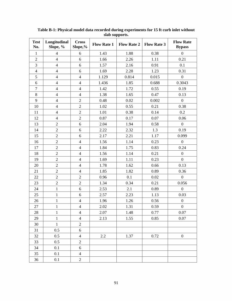
91
Table B-1: Physical model data recorded during experiments for 15 ft curb inlet without
slab supports.
Test
No.
Longitudinal
Slope, %
Cross
Slope,% Flow Rate 1 Flow Rate 2 Flow Rate 3
Flow Rate
Bypass
1 4 6 1.43 1.88 0.38 0
2 4 6 1.66 2.26 1.11 0.21
3 4 6 1.57 2.16 0.91 0.1
4 4 6 1.69 2.28 1.23 0.31
5 4 4 1.129 0.814 0.015 0
6 4 4 1.436 1.85 0.688 0.3043
7 4 4 1.42 1.72 0.55 0.19
8 4 4 1.38 1.65 0.47 0.13
9 4 2 0.48 0.02 0.002 0
10 4 2 1.02 0.55 0.21 0.38
11 4 2 1.01 0.38 0.14 0.2
12 4 2 0.87 0.17 0.07 0.06
13 2 6 2.04 1.94 0.58 0
14 2 6 2.22 2.32 1.3 0.19
15 2 6 2.17 2.21 1.17 0.099
16 2 4 1.56 1.14 0.23 0
17 2 4 1.84 1.75 0.83 0.24
18 2 4 1.56 1.14 0.21 0
19 2 4 1.69 1.11 0.23 0
20 2 4 1.78 1.62 0.66 0.13
21 2 4 1.85 1.82 0.89 0.36
22 2 2 0.96 0.1 0.02 0
23 2 2 1.34 0.34 0.21 0.056
24 1 6 2.53 2.1 0.89 0
25 1 6 2.57 2.23 1.13 0.03
26 1 4 1.96 1.26 0.56 0
27 1 4 2.02 1.31 0.59 0
28 1 4 2.07 1.48 0.77 0.07
29 1 4 2.13 1.55 0.85 0.07
30 1 2
31 0.5 6
32 0.5 4 2.2 1.37 0.72 0
33 0.5 2
34 0.1 6
35 0.1 4
36 0.1 2
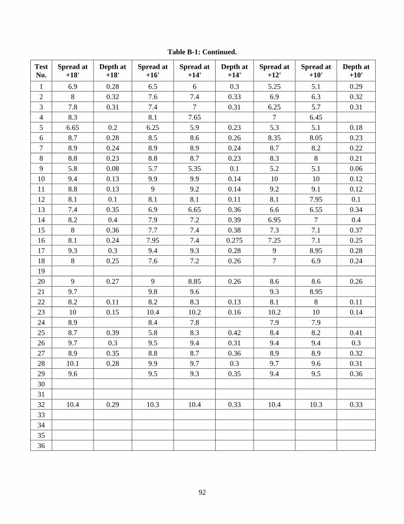
92
Table B-1: Continued.
Test
No.
Spread at
+18'
Depth at
+18'
Spread at
+16'
Spread at
+14'
Depth at
+14'
Spread at
+12'
Spread at
+10'
Depth at
+10'
1 6.9 0.28 6.5 6 0.3 5.25 5.1 0.29
2 8 0.32 7.6 7.4 0.33 6.9 6.3 0.32
3 7.8 0.31 7.4 7 0.31 6.25 5.7 0.31
4 8.3 8.1 7.65 7 6.45
5 6.65 0.2 6.25 5.9 0.23 5.3 5.1 0.18
6 8.7 0.28 8.5 8.6 0.26 8.35 8.05 0.23
7 8.9 0.24 8.9 8.9 0.24 8.7 8.2 0.22
8 8.8 0.23 8.8 8.7 0.23 8.3 8 0.21
9 5.8 0.08 5.7 5.35 0.1 5.2 5.1 0.06
10 9.4 0.13 9.9 9.9 0.14 10 10 0.12
11 8.8 0.13 9 9.2 0.14 9.2 9.1 0.12
12 8.1 0.1 8.1 8.1 0.11 8.1 7.95 0.1
13 7.4 0.35 6.9 6.65 0.36 6.6 6.55 0.34
14 8.2 0.4 7.9 7.2 0.39 6.95 7 0.4
15 8 0.36 7.7 7.4 0.38 7.3 7.1 0.37
16 8.1 0.24 7.95 7.4 0.275 7.25 7.1 0.25
17 9.3 0.3 9.4 9.3 0.28 9 8.95 0.28
18 8 0.25 7.6 7.2 0.26 7 6.9 0.24
19
20 9 0.27 9 8.85 0.26 8.6 8.6 0.26
21 9.7 9.8 9.6 9.3 8.95
22 8.2 0.11 8.2 8.3 0.13 8.1 8 0.11
23 10 0.15 10.4 10.2 0.16 10.2 10 0.14
24 8.9 8.4 7.8 7.9 7.9
25 8.7 0.39 5.8 8.3 0.42 8.4 8.2 0.41
26 9.7 0.3 9.5 9.4 0.31 9.4 9.4 0.3
27 8.9 0.35 8.8 8.7 0.36 8.9 8.9 0.32
28 10.1 0.28 9.9 9.7 0.3 9.7 9.6 0.31
29 9.6 9.5 9.3 0.35 9.4 9.5 0.36
30
31
32 10.4 0.29 10.3 10.4 0.33 10.4 10.3 0.33
33
34
35
36
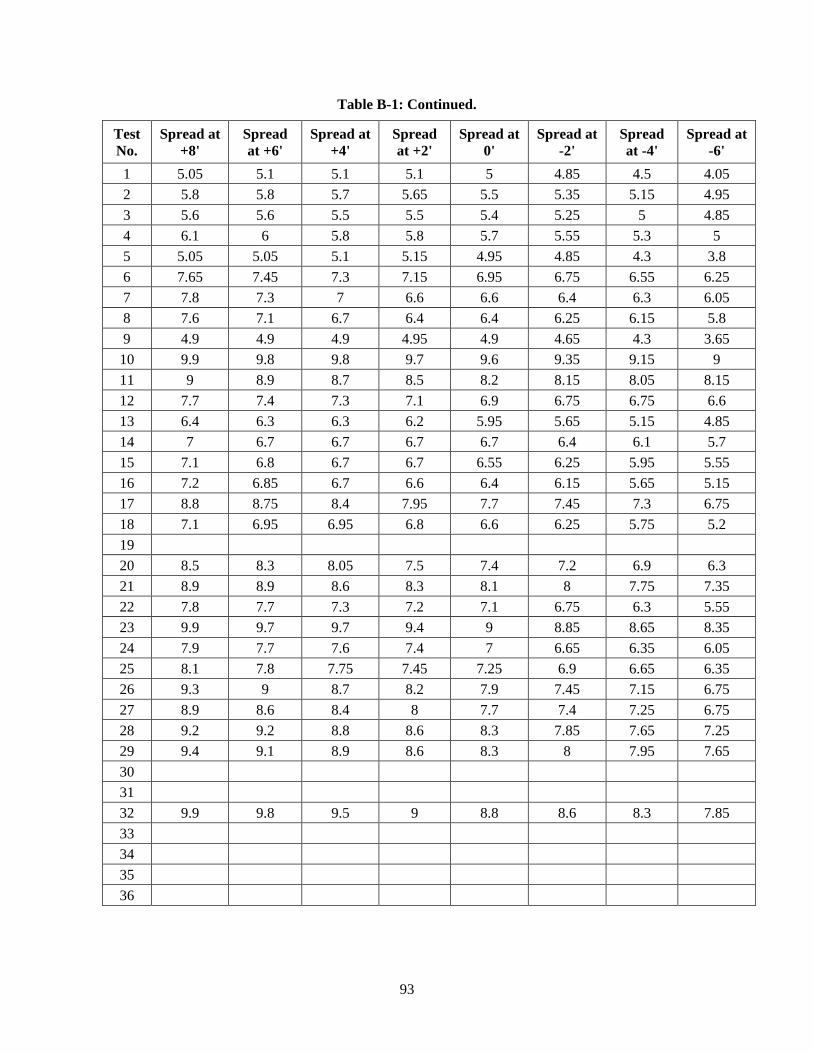
93
Table B-1: Continued.
Test
No.
Spread at
+8'
Spread
at +6'
Spread at
+4'
Spread
at +2'
Spread at
0'
Spread at
-2'
Spread
at -4'
Spread at
-6'
1 5.05 5.1 5.1 5.1 5 4.85 4.5 4.05
2 5.8 5.8 5.7 5.65 5.5 5.35 5.15 4.95
3 5.6 5.6 5.5 5.5 5.4 5.25 5 4.85
4 6.1 6 5.8 5.8 5.7 5.55 5.3 5
5 5.05 5.05 5.1 5.15 4.95 4.85 4.3 3.8
6 7.65 7.45 7.3 7.15 6.95 6.75 6.55 6.25
7 7.8 7.3 7 6.6 6.6 6.4 6.3 6.05
8 7.6 7.1 6.7 6.4 6.4 6.25 6.15 5.8
9 4.9 4.9 4.9 4.95 4.9 4.65 4.3 3.65
10 9.9 9.8 9.8 9.7 9.6 9.35 9.15 9
11 9 8.9 8.7 8.5 8.2 8.15 8.05 8.15
12 7.7 7.4 7.3 7.1 6.9 6.75 6.75 6.6
13 6.4 6.3 6.3 6.2 5.95 5.65 5.15 4.85
14 7 6.7 6.7 6.7 6.7 6.4 6.1 5.7
15 7.1 6.8 6.7 6.7 6.55 6.25 5.95 5.55
16 7.2 6.85 6.7 6.6 6.4 6.15 5.65 5.15
17 8.8 8.75 8.4 7.95 7.7 7.45 7.3 6.75
18 7.1 6.95 6.95 6.8 6.6 6.25 5.75 5.2
19
20 8.5 8.3 8.05 7.5 7.4 7.2 6.9 6.3
21 8.9 8.9 8.6 8.3 8.1 8 7.75 7.35
22 7.8 7.7 7.3 7.2 7.1 6.75 6.3 5.55
23 9.9 9.7 9.7 9.4 9 8.85 8.65 8.35
24 7.9 7.7 7.6 7.4 7 6.65 6.35 6.05
25 8.1 7.8 7.75 7.45 7.25 6.9 6.65 6.35
26 9.3 9 8.7 8.2 7.9 7.45 7.15 6.75
27 8.9 8.6 8.4 8 7.7 7.4 7.25 6.75
28 9.2 9.2 8.8 8.6 8.3 7.85 7.65 7.25
29 9.4 9.1 8.9 8.6 8.3 8 7.95 7.65
30
31
32 9.9 9.8 9.5 9 8.8 8.6 8.3 7.85
33
34
35
36
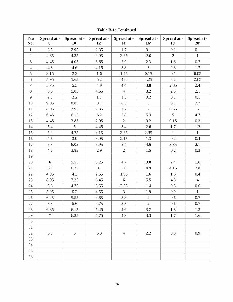
94
Table B-1: Continued
Test
No.
Spread at -
8'
Spread at -
10'
Spread at -
12'
Spread at -
14'
Spread at -
16'
Spread at -
18'
Spread at -
20'
1 3.5 2.95 2.35 1.7 0.1 0.1 0.1
2 4.65 4.35 3.95 3.35 2.6 2 1
3 4.45 4.05 3.65 2.9 2.3 1.6 0.7
4 4.8 4.6 4.15 3.8 3 2.3 1.7
5 3.15 2.2 1.6 1.45 0.15 0.1 0.05
6 5.95 5.65 5.2 4.8 4.25 3.2 2.65
7 5.75 5.3 4.9 4.4 3.8 2.85 2.4
8 5.6 5.05 4.55 4 3.2 2.5 2.1
9 2.8 2.2 1.7 1.5 0.2 0.1 0.1
10 9.05 8.85 8.7 8.3 8 8.1 7.7
11 8.05 7.95 7.35 7.2 7 6.55 6
12 6.45 6.15 6.2 5.8 5.3 5 4.7
13 4.45 3.85 2.95 2 0.2 0.15 0.3
14 5.4 5 4.45 3.4 2.6 1.7 1.2
15 5.3 4.75 4.15 3.35 2.35 1 1
16 4.6 3.9 3.05 2.15 1.3 0.2 0.4
17 6.3 6.05 5.95 5.4 4.6 3.35 2.1
18 4.6 3.85 2.9 2 1.5 0.2 0.3
19
20 6 5.55 5.25 4.7 3.8 2.4 1.6
21 6.7 6.25 6 5.6 4.9 4.15 2.8
22 4.95 4.3 2.55 1.95 1.6 1.6 0.4
23 8.05 7.25 6.45 6 5.5 4.8 4
24 5.6 4.75 3.65 2.55 1.4 0.5 0.6
25 5.95 5.2 4.55 3 1.9 0.9 1
26 6.25 5.55 4.65 3.3 2 0.6 0.7
27 6.3 5.6 4.75 3.5 2 0.6 0.7
28 6.85 6.15 5.45 4.6 3.2 1.8 1.3
29 7 6.35 5.75 4.9 3.3 1.7 1.6
30
31
32 6.9 6 5.3 4 2.2 0.8 0.9
33
34
35
36
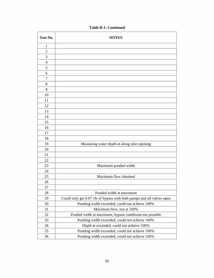
95
Table B-1: Continued
Test No. NOTES
1
2
3
4
5
6
7
8
9
10
11
12
13
14
15
16
17
18
19 Measuring water depth at along inlet opening
20
21
22
23 Maximum ponded width
24
25 Maximum flow obtained
26
27
28 Ponded width at maximum
29 Could only get 0.07 cfs of bypass with both pumps and all valves open
30 Ponding width exceeded, could not achieve 100%
31 Maximum flow, not at 100%
32 Ponded width at maximum, bypass conditions not possible
33 Ponding width exceeded, could not achieve 100%
34 Depth at exceeded, could not achieve 100%
35 Ponding width exceeded, could not achieve 100%
36 Ponding width exceeded, could not achieve 100%
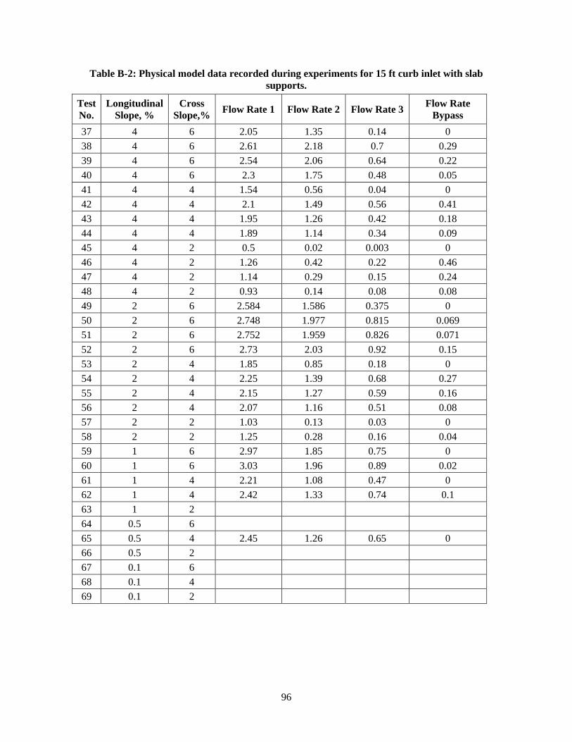
96
Table B-2: Physical model data recorded during experiments for 15 ft curb inlet with slab
supports.
Test
No.
Longitudinal
Slope, %
Cross
Slope,% Flow Rate 1 Flow Rate 2 Flow Rate 3
Flow Rate
Bypass
37 4 6 2.05 1.35 0.14 0
38 4 6 2.61 2.18 0.7 0.29
39 4 6 2.54 2.06 0.64 0.22
40 4 6 2.3 1.75 0.48 0.05
41 4 4 1.54 0.56 0.04 0
42 4 4 2.1 1.49 0.56 0.41
43 4 4 1.95 1.26 0.42 0.18
44 4 4 1.89 1.14 0.34 0.09
45 4 2 0.5 0.02 0.003 0
46 4 2 1.26 0.42 0.22 0.46
47 4 2 1.14 0.29 0.15 0.24
48 4 2 0.93 0.14 0.08 0.08
49 2 6 2.584 1.586 0.375 0
50 2 6 2.748 1.977 0.815 0.069
51 2 6 2.752 1.959 0.826 0.071
52 2 6 2.73 2.03 0.92 0.15
53 2 4 1.85 0.85 0.18 0
54 2 4 2.25 1.39 0.68 0.27
55 2 4 2.15 1.27 0.59 0.16
56 2 4 2.07 1.16 0.51 0.08
57 2 2 1.03 0.13 0.03 0
58 2 2 1.25 0.28 0.16 0.04
59 1 6 2.97 1.85 0.75 0
60 1 6 3.03 1.96 0.89 0.02
61 1 4 2.21 1.08 0.47 0
62 1 4 2.42 1.33 0.74 0.1
63 1 2
64 0.5 6
65 0.5 4 2.45 1.26 0.65 0
66 0.5 2
67 0.1 6
68 0.1 4
69 0.1 2
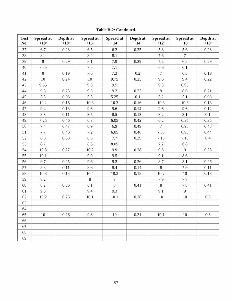
97
Table B-2: Continued.
Test
No.
Spread at
+18'
Depth at
+18'
Spread at
+16'
Spread at
+14'
Depth at
+14'
Spread at
+12'
Spread at
+10'
Depth at
+10'
37 6.7 0.23 6.5 6.2 0.25 5.8 5.6 0.28
38 8.2 8.2 8.1 7.6 7
39 8 0.29 8.1 7.9 0.29 7.3 6.8 0.29
40 7.75 7.5 7.1 6.6 6.1
41 8 0.19 7.6 7.3 0.2 7 6.3 0.19
42 10 0.24 10 9.75 0.25 9.6 9.4 0.22
43 9.55 9.6 9.5 9.3 8.95
44 9.3 0.23 9.3 9.2 0.23 9 8.6 0.21
45 5.5 0.08 5.5 5.25 0.1 5.2 5.1 0.08
46 10.2 0.16 10.3 10.3 0.16 10.3 10.3 0.13
47 9.4 0.13 9.6 9.6 0.14 9.6 9.6 0.12
48 8.3 0.11 8.5 8.5 0.13 8.2 8.1 0.1
49 7.25 0.46 6.3 6.05 0.42 6.2 6.35 0.35
50 7.4 0.47 6.9 6.9 0.49 7 6.95 0.43
51 7.7 0.46 7.2 6.05 0.46 7.05 6.95 0.44
52 8.8 0.38 8.5 7.7 0.39 7.15 7.15 0.4
53 8.7 8.6 8.05 7.2 6.8
54 10.3 0.27 10.2 9.9 0.28 9.5 9 0.28
55 10.1 9.9 9.5 9.1 8.6
56 9.7 0.25 9.6 9.3 0.26 8.7 8.1 0.26
57 8.3 0.11 8.6 8.4 0.14 8 7.9 0.11
58 10.3 0.15 10.4 10.3 0.15 10.2 10 0.13
59 8.2 8 8 7.9 7.8
60 8.2 0.36 8.1 8 0.41 8 7.8 0.41
61 9.5 9.4 9.3 9.1 9
62 10.2 0.25 10.1 10.1 0.28 10 10 0.3
63
64
65 10 0.26 9.8 10 0.31 10.1 10 0.3
66
67
68
69
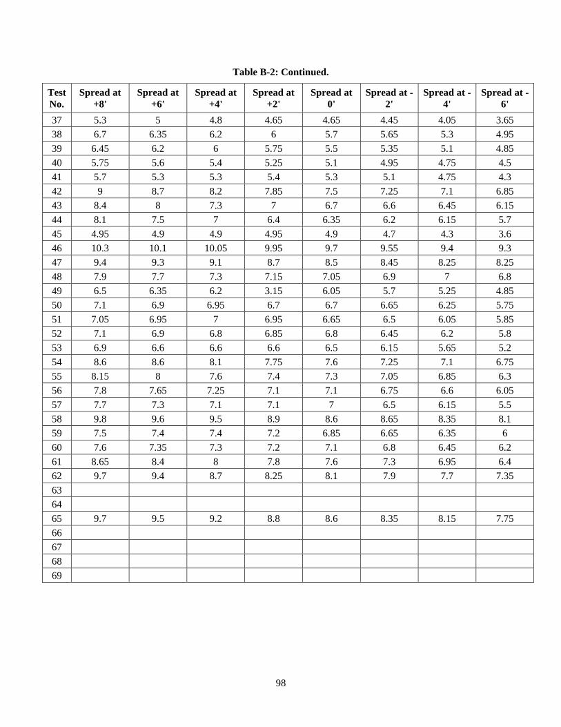
98
Table B-2: Continued.
Test
No.
Spread at
+8'
Spread at
+6'
Spread at
+4'
Spread at
+2'
Spread at
0'
Spread at -
2'
Spread at -
4'
Spread at -
6'
37 5.3 5 4.8 4.65 4.65 4.45 4.05 3.65
38 6.7 6.35 6.2 6 5.7 5.65 5.3 4.95
39 6.45 6.2 6 5.75 5.5 5.35 5.1 4.85
40 5.75 5.6 5.4 5.25 5.1 4.95 4.75 4.5
41 5.7 5.3 5.3 5.4 5.3 5.1 4.75 4.3
42 9 8.7 8.2 7.85 7.5 7.25 7.1 6.85
43 8.4 8 7.3 7 6.7 6.6 6.45 6.15
44 8.1 7.5 7 6.4 6.35 6.2 6.15 5.7
45 4.95 4.9 4.9 4.95 4.9 4.7 4.3 3.6
46 10.3 10.1 10.05 9.95 9.7 9.55 9.4 9.3
47 9.4 9.3 9.1 8.7 8.5 8.45 8.25 8.25
48 7.9 7.7 7.3 7.15 7.05 6.9 7 6.8
49 6.5 6.35 6.2 3.15 6.05 5.7 5.25 4.85
50 7.1 6.9 6.95 6.7 6.7 6.65 6.25 5.75
51 7.05 6.95 7 6.95 6.65 6.5 6.05 5.85
52 7.1 6.9 6.8 6.85 6.8 6.45 6.2 5.8
53 6.9 6.6 6.6 6.6 6.5 6.15 5.65 5.2
54 8.6 8.6 8.1 7.75 7.6 7.25 7.1 6.75
55 8.15 8 7.6 7.4 7.3 7.05 6.85 6.3
56 7.8 7.65 7.25 7.1 7.1 6.75 6.6 6.05
57 7.7 7.3 7.1 7.1 7 6.5 6.15 5.5
58 9.8 9.6 9.5 8.9 8.6 8.65 8.35 8.1
59 7.5 7.4 7.4 7.2 6.85 6.65 6.35 6
60 7.6 7.35 7.3 7.2 7.1 6.8 6.45 6.2
61 8.65 8.4 8 7.8 7.6 7.3 6.95 6.4
62 9.7 9.4 8.7 8.25 8.1 7.9 7.7 7.35
63
64
65 9.7 9.5 9.2 8.8 8.6 8.35 8.15 7.75
66
67
68
69
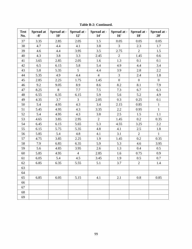
99
Table B-2: Continued.
Test
No.
Spread at
-8'
Spread at -
10'
Spread at -
12'
Spread at -
14'
Spread at -
16'
Spread at -
18'
Spread at -
20'
37 3.35 2.85 2.05 1.5 0.05 0.05 0.05
38 4.7 4.4 4.1 3.8 3 2.3 1.7
39 4.6 4.4 3.95 3.5 2.75 2 1.5
40 4.3 3.8 3.3 2.45 2 1.45 0.6
41 3.65 2.85 2.05 1.6 1.3 0.1 0.1
42 6.5 6.15 5.8 5.4 4.9 4.4 3.4
43 5.8 5.35 5 4.4 3.9 2.8 2.2
44 5.35 4.9 4.4 4 3 2.4 1.8
45 2.85 2.25 1.75 1.45 0 0 0
46 9.2 9.05 8.9 8.6 8.2 8.1 7.9
47 8.25 8 7.7 7.5 7.3 6.7 6.3
48 6.55 6.35 6.15 5.9 5.6 5.2 4.9
49 4.35 3.7 3 2.05 0.3 0.25 0.1
50 5.4 4.95 4.3 3.4 2.15 0.85 1
51 5.45 4.95 4.3 3.35 2.2 0.95 1
52 5.4 4.95 4.3 3.8 2.5 1.5 1.1
53 4.65 3.85 2.95 2 1.45 0.2 0.35
54 6.45 6.15 5.65 5.3 4.55 3.25 2.2
55 6.15 5.75 5.35 4.8 4.1 2.5 1.8
56 5.85 5.4 4.8 4.1 3.1 2 1
57 4.75 3.85 2.25 1.9 1.45 0.2 0.35
58 7.9 6.85 6.35 5.9 5.3 4.6 3.95
59 5.6 4.85 3.95 2.6 1.3 0.4 0.5
60 5.85 4.95 4 2.85 1.6 0.75 0.9
61 6.05 5.4 4.5 3.45 1.9 0.5 0.7
62 6.85 6.35 5.55 5.1 3.7 2 1.4
63
64
65 6.85 6.05 5.15 4.1 2.1 0.8 0.85
66
67
68
69
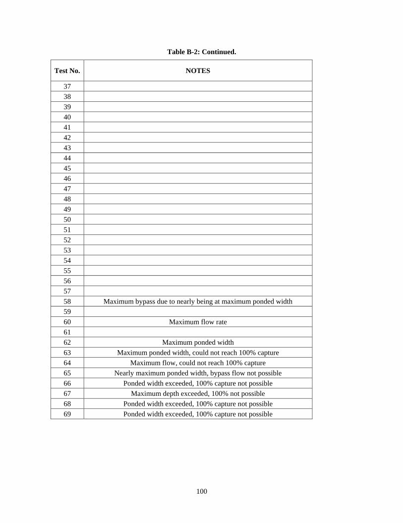
100
Table B-2: Continued.
Test No. NOTES
37
38
39
40
41
42
43
44
45
46
47
48
49
50
51
52
53
54
55
56
57
58 Maximum bypass due to nearly being at maximum ponded width
59
60 Maximum flow rate
61
62 Maximum ponded width
63 Maximum ponded width, could not reach 100% capture
64 Maximum flow, could not reach 100% capture
65 Nearly maximum ponded width, bypass flow not possible
66 Ponded width exceeded, 100% capture not possible
67 Maximum depth exceeded, 100% not possible
68 Ponded width exceeded, 100% capture not possible
69 Ponded width exceeded, 100% capture not possible

101
Table B-3: Physical model data recorded during experiments for 10 ft curb inlet without
slab supports.
Test
No.
Longitudinal
Slope, %
Cross
Slope,% Flow Rate 1 Flow Rate 2
Flow Rate
Bypass
70 4 6 1.42 1.21 0
71 4 6 1.66 2.5 0.55
72 4 6 1.57 2.24 0.33
73 4 6 1.48 1.98 0.13
74 4 4 1.14 0.53 0
75 4 4 1.41 1.78 0.48
76 4 4 1.35 1.59 0.3
77 4 4 1.28 1.23 0.09
78 4 2 0.435 0.005 0
79 4 2 1.05 0.54 0.49
80 4 2 1.02 0.39 0.3
81 4 2 0.9 0.13 0.1
82 2 6 1.84 1.18 0
83 2 6 2.1 2.24 0.49
84 2 6 2.04 2.04 0.3
85 2 6 1.94 1.68 0.1
86 2 4 1.51 0.68 0
87 2 4 1.78 1.62 0.47
88 2 4 1.65 1.44 0.3
89 2 4 1.6 1.15 0.09
90 2 2 0.86 0.06 0
91 2 2 1.22 0.29 0.09
92 2 2 1.3 0.52 0.27
93 1 6 2.12 1.2 0
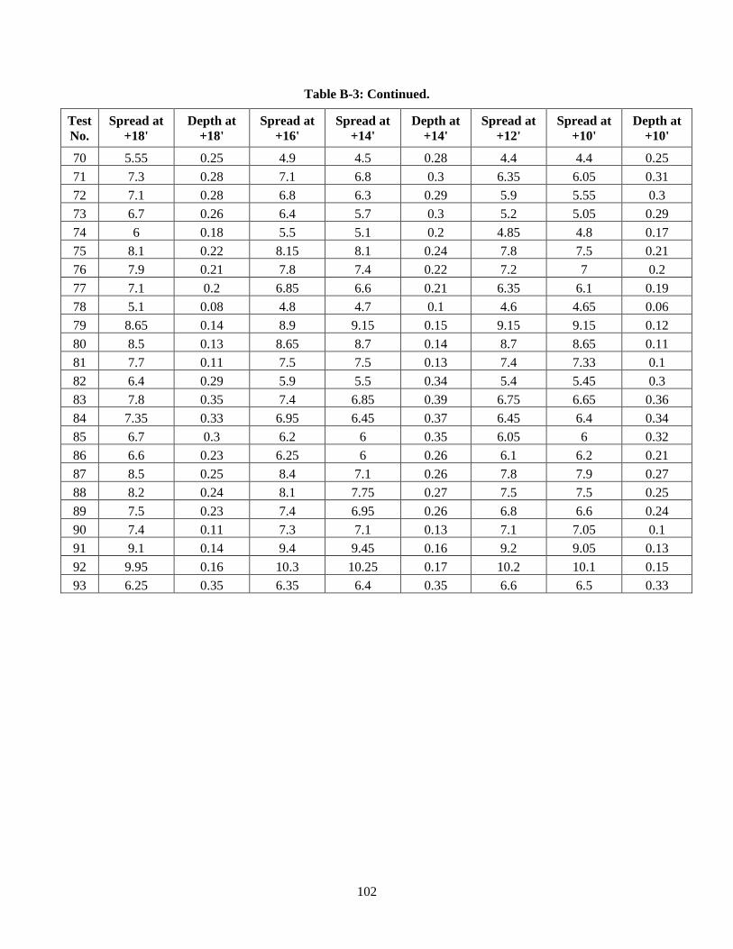
102
Table B-3: Continued.
Test
No.
Spread at
+18'
Depth at
+18'
Spread at
+16'
Spread at
+14'
Depth at
+14'
Spread at
+12'
Spread at
+10'
Depth at
+10'
70 5.55 0.25 4.9 4.5 0.28 4.4 4.4 0.25
71 7.3 0.28 7.1 6.8 0.3 6.35 6.05 0.31
72 7.1 0.28 6.8 6.3 0.29 5.9 5.55 0.3
73 6.7 0.26 6.4 5.7 0.3 5.2 5.05 0.29
74 6 0.18 5.5 5.1 0.2 4.85 4.8 0.17
75 8.1 0.22 8.15 8.1 0.24 7.8 7.5 0.21
76 7.9 0.21 7.8 7.4 0.22 7.2 7 0.2
77 7.1 0.2 6.85 6.6 0.21 6.35 6.1 0.19
78 5.1 0.08 4.8 4.7 0.1 4.6 4.65 0.06
79 8.65 0.14 8.9 9.15 0.15 9.15 9.15 0.12
80 8.5 0.13 8.65 8.7 0.14 8.7 8.65 0.11
81 7.7 0.11 7.5 7.5 0.13 7.4 7.33 0.1
82 6.4 0.29 5.9 5.5 0.34 5.4 5.45 0.3
83 7.8 0.35 7.4 6.85 0.39 6.75 6.65 0.36
84 7.35 0.33 6.95 6.45 0.37 6.45 6.4 0.34
85 6.7 0.3 6.2 6 0.35 6.05 6 0.32
86 6.6 0.23 6.25 6 0.26 6.1 6.2 0.21
87 8.5 0.25 8.4 7.1 0.26 7.8 7.9 0.27
88 8.2 0.24 8.1 7.75 0.27 7.5 7.5 0.25
89 7.5 0.23 7.4 6.95 0.26 6.8 6.6 0.24
90 7.4 0.11 7.3 7.1 0.13 7.1 7.05 0.1
91 9.1 0.14 9.4 9.45 0.16 9.2 9.05 0.13
92 9.95 0.16 10.3 10.25 0.17 10.2 10.1 0.15
93 6.25 0.35 6.35 6.4 0.35 6.6 6.5 0.33
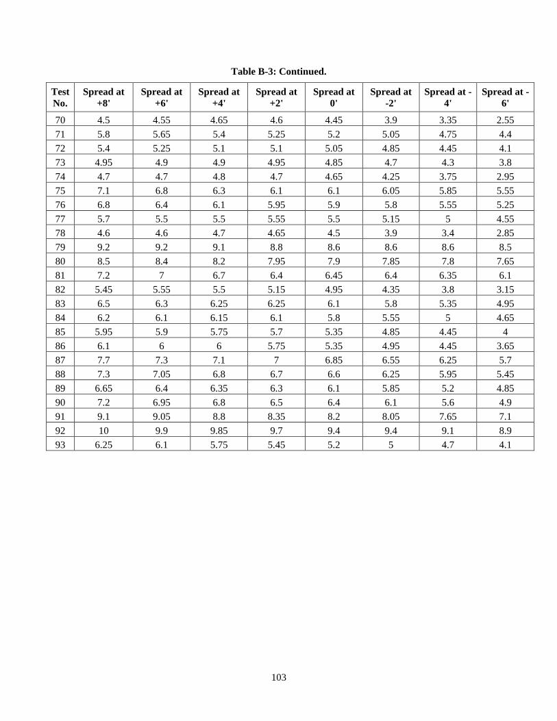
103
Table B-3: Continued.
Test
No.
Spread at
+8'
Spread at
+6'
Spread at
+4'
Spread at
+2'
Spread at
0'
Spread at
-2'
Spread at -
4'
Spread at -
6'
70 4.5 4.55 4.65 4.6 4.45 3.9 3.35 2.55
71 5.8 5.65 5.4 5.25 5.2 5.05 4.75 4.4
72 5.4 5.25 5.1 5.1 5.05 4.85 4.45 4.1
73 4.95 4.9 4.9 4.95 4.85 4.7 4.3 3.8
74 4.7 4.7 4.8 4.7 4.65 4.25 3.75 2.95
75 7.1 6.8 6.3 6.1 6.1 6.05 5.85 5.55
76 6.8 6.4 6.1 5.95 5.9 5.8 5.55 5.25
77 5.7 5.5 5.5 5.55 5.5 5.15 5 4.55
78 4.6 4.6 4.7 4.65 4.5 3.9 3.4 2.85
79 9.2 9.2 9.1 8.8 8.6 8.6 8.6 8.5
80 8.5 8.4 8.2 7.95 7.9 7.85 7.8 7.65
81 7.2 7 6.7 6.4 6.45 6.4 6.35 6.1
82 5.45 5.55 5.5 5.15 4.95 4.35 3.8 3.15
83 6.5 6.3 6.25 6.25 6.1 5.8 5.35 4.95
84 6.2 6.1 6.15 6.1 5.8 5.55 5 4.65
85 5.95 5.9 5.75 5.7 5.35 4.85 4.45 4
86 6.1 6 6 5.75 5.35 4.95 4.45 3.65
87 7.7 7.3 7.1 7 6.85 6.55 6.25 5.7
88 7.3 7.05 6.8 6.7 6.6 6.25 5.95 5.45
89 6.65 6.4 6.35 6.3 6.1 5.85 5.2 4.85
90 7.2 6.95 6.8 6.5 6.4 6.1 5.6 4.9
91 9.1 9.05 8.8 8.35 8.2 8.05 7.65 7.1
92 10 9.9 9.85 9.7 9.4 9.4 9.1 8.9
93 6.25 6.1 5.75 5.45 5.2 5 4.7 4.1
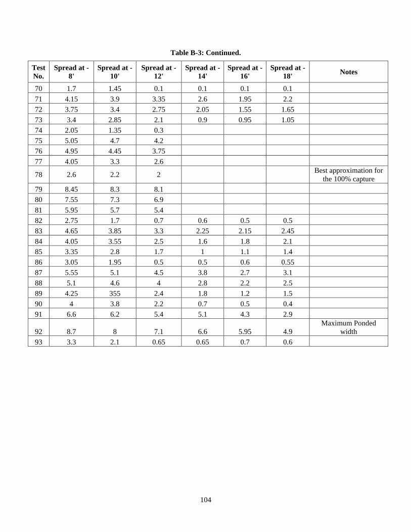
104
Table B-3: Continued.
Test
No.
Spread at -
8'
Spread at -
10'
Spread at -
12'
Spread at -
14'
Spread at -
16'
Spread at -
18' Notes
70 1.7 1.45 0.1 0.1 0.1 0.1
71 4.15 3.9 3.35 2.6 1.95 2.2
72 3.75 3.4 2.75 2.05 1.55 1.65
73 3.4 2.85 2.1 0.9 0.95 1.05
74 2.05 1.35 0.3
75 5.05 4.7 4.2
76 4.95 4.45 3.75
77 4.05 3.3 2.6
78 2.6 2.2 2 Best approximation for
the 100% capture
79 8.45 8.3 8.1
80 7.55 7.3 6.9
81 5.95 5.7 5.4
82 2.75 1.7 0.7 0.6 0.5 0.5
83 4.65 3.85 3.3 2.25 2.15 2.45
84 4.05 3.55 2.5 1.6 1.8 2.1
85 3.35 2.8 1.7 1 1.1 1.4
86 3.05 1.95 0.5 0.5 0.6 0.55
87 5.55 5.1 4.5 3.8 2.7 3.1
88 5.1 4.6 4 2.8 2.2 2.5
89 4.25 355 2.4 1.8 1.2 1.5
90 4 3.8 2.2 0.7 0.5 0.4
91 6.6 6.2 5.4 5.1 4.3 2.9
92 8.7 8 7.1 6.6 5.95 4.9
Maximum Ponded
width
93 3.3 2.1 0.65 0.65 0.7 0.6
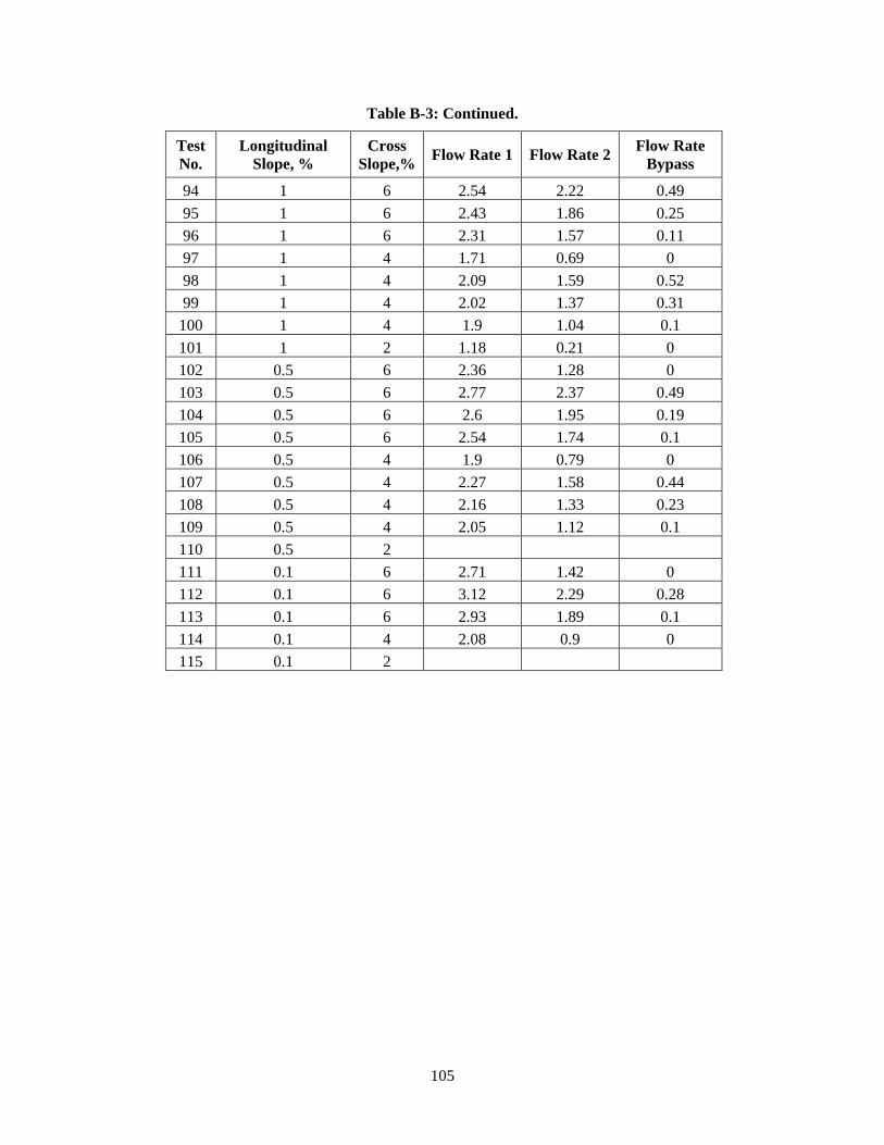
105
Table B-3: Continued.
Test
No.
Longitudinal
Slope, %
Cross
Slope,% Flow Rate 1 Flow Rate 2
Flow Rate
Bypass
94 1 6 2.54 2.22 0.49
95 1 6 2.43 1.86 0.25
96 1 6 2.31 1.57 0.11
97 1 4 1.71 0.69 0
98 1 4 2.09 1.59 0.52
99 1 4 2.02 1.37 0.31
100 1 4 1.9 1.04 0.1
101 1 2 1.18 0.21 0
102 0.5 6 2.36 1.28 0
103 0.5 6 2.77 2.37 0.49
104 0.5 6 2.6 1.95 0.19
105 0.5 6 2.54 1.74 0.1
106 0.5 4 1.9 0.79 0
107 0.5 4 2.27 1.58 0.44
108 0.5 4 2.16 1.33 0.23
109 0.5 4 2.05 1.12 0.1
110 0.5 2
111 0.1 6 2.71 1.42 0
112 0.1 6 3.12 2.29 0.28
113 0.1 6 2.93 1.89 0.1
114 0.1 4 2.08 0.9 0
115 0.1 2
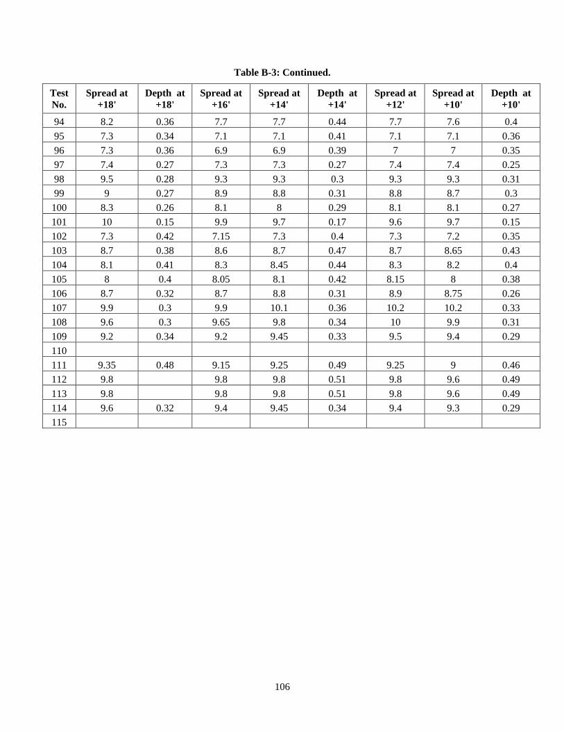
106
Table B-3: Continued.
Test
No.
Spread at
+18'
Depth at
+18'
Spread at
+16'
Spread at
+14'
Depth at
+14'
Spread at
+12'
Spread at
+10'
Depth at
+10'
94 8.2 0.36 7.7 7.7 0.44 7.7 7.6 0.4
95 7.3 0.34 7.1 7.1 0.41 7.1 7.1 0.36
96 7.3 0.36 6.9 6.9 0.39 7 7 0.35
97 7.4 0.27 7.3 7.3 0.27 7.4 7.4 0.25
98 9.5 0.28 9.3 9.3 0.3 9.3 9.3 0.31
99 9 0.27 8.9 8.8 0.31 8.8 8.7 0.3
100 8.3 0.26 8.1 8 0.29 8.1 8.1 0.27
101 10 0.15 9.9 9.7 0.17 9.6 9.7 0.15
102 7.3 0.42 7.15 7.3 0.4 7.3 7.2 0.35
103 8.7 0.38 8.6 8.7 0.47 8.7 8.65 0.43
104 8.1 0.41 8.3 8.45 0.44 8.3 8.2 0.4
105 8 0.4 8.05 8.1 0.42 8.15 8 0.38
106 8.7 0.32 8.7 8.8 0.31 8.9 8.75 0.26
107 9.9 0.3 9.9 10.1 0.36 10.2 10.2 0.33
108 9.6 0.3 9.65 9.8 0.34 10 9.9 0.31
109 9.2 0.34 9.2 9.45 0.33 9.5 9.4 0.29
110
111 9.35 0.48 9.15 9.25 0.49 9.25 9 0.46
112 9.8 9.8 9.8 0.51 9.8 9.6 0.49
113 9.8 9.8 9.8 0.51 9.8 9.6 0.49
114 9.6 0.32 9.4 9.45 0.34 9.4 9.3 0.29
115
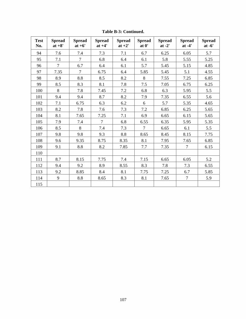
107
Table B-3: Continued.
Test
No.
Spread
at +8'
Spread
at +6'
Spread
at +4'
Spread
at +2'
Spread
at 0'
Spread
at -2'
Spread
at -4'
Spread
at -6'
94 7.6 7.4 7.3 7.1 6.7 6.25 6.05 5.7
95 7.1 7 6.8 6.4 6.1 5.8 5.55 5.25
96 7 6.7 6.4 6.1 5.7 5.45 5.15 4.85
97 7.35 7 6.75 6.4 5.85 5.45 5.1 4.55
98 8.9 8.8 8.5 8.2 8 7.55 7.25 6.85
99 8.5 8.3 8.1 7.8 7.5 7.05 6.75 6.25
100 8 7.8 7.45 7.2 6.8 6.3 5.95 5.5
101 9.4 9.4 8.7 8.2 7.9 7.35 6.55 5.6
102 7.1 6.75 6.3 6.2 6 5.7 5.35 4.65
103 8.2 7.8 7.6 7.3 7.2 6.85 6.25 5.65
104 8.1 7.65 7.25 7.1 6.9 6.65 6.15 5.65
105 7.9 7.4 7 6.8 6.55 6.35 5.95 5.35
106 8.5 8 7.4 7.3 7 6.65 6.1 5.5
107 9.8 9.8 9.3 8.8 8.65 8.45 8.15 7.75
108 9.6 9.35 8.75 8.35 8.1 7.95 7.65 6.85
109 9.1 8.8 8.2 7.85 7.7 7.35 7 6.15
110
111 8.7 8.15 7.75 7.4 7.15 6.65 6.05 5.2
112 9.4 9.2 8.9 8.55 8.3 7.8 7.3 6.55
113 9.2 8.85 8.4 8.1 7.75 7.25 6.7 5.85
114 9 8.8 8.65 8.3 8.1 7.65 7 5.9
115
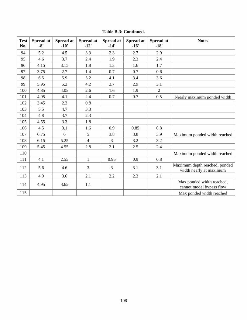
108
Table B-3: Continued.
Test
No.
Spread at
-8'
Spread at
-10'
Spread at
-12'
Spread at
-14'
Spread at
-16'
Spread at
-18'
Notes
94 5.2 4.5 3.3 2.3 2.7 2.9
95 4.6 3.7 2.4 1.9 2.3 2.4
96 4.15 3.15 1.8 1.3 1.6 1.7
97 3.75 2.7 1.4 0.7 0.7 0.6
98 6.5 5.9 5.2 4.1 3.4 3.6
99 5.95 5.2 4.2 2.7 2.9 3.1
100 4.85 4.05 2.6 1.6 1.9 2
101 4.95 4.1 2.4 0.7 0.7 0.5 Nearly maximum ponded width
102 3.45 2.3 0.8
103 5.5 4.7 3.3
104 4.8 3.7 2.3
105 4.55 3.3 1.8
106 4.5 3.1 1.6 0.9 0.85 0.8
107 6.75 6 5 3.8 3.8 3.9 Maximum ponded width reached
108 6.15 5.25 4 3 3.2 3.2
109 5.45 4.55 2.8 2.1 2.5 2.4
110 Maximum ponded width reached
111 4.1 2.55 1 0.95 0.9 0.8
112 5.6 4.6 3 3 3.1 3.1 Maximum depth reached, ponded
width nearly at maximum
113 4.9 3.6 2.1 2.2 2.3 2.1
114 4.95 3.65 1.1 Max ponded width reached,
cannot model bypass flow
115 Max ponded width reached
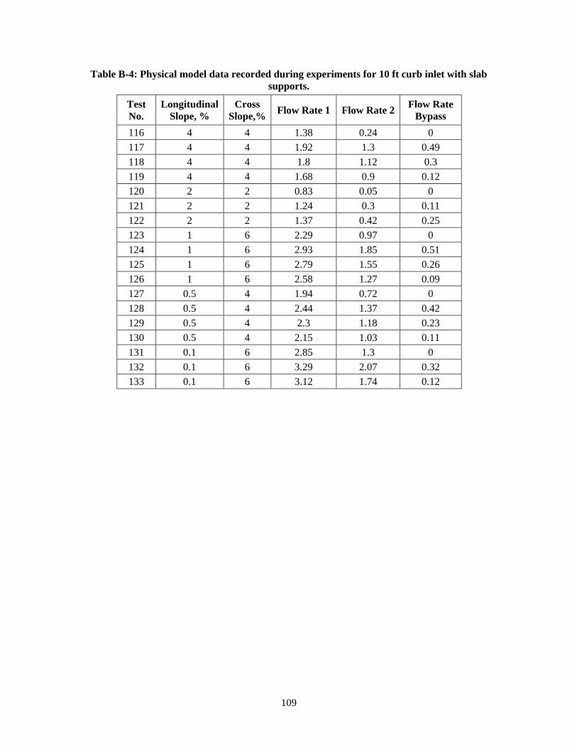
109
Table B-4: Physical model data recorded during experiments for 10 ft curb inlet with slab
supports.
Test
No.
Longitudinal
Slope, %
Cross
Slope,% Flow Rate 1 Flow Rate 2
Flow Rate
Bypass
116 4 4 1.38 0.24 0
117 4 4 1.92 1.3 0.49
118 4 4 1.8 1.12 0.3
119 4 4 1.68 0.9 0.12
120 2 2 0.83 0.05 0
121 2 2 1.24 0.3 0.11
122 2 2 1.37 0.42 0.25
123 1 6 2.29 0.97 0
124 1 6 2.93 1.85 0.51
125 1 6 2.79 1.55 0.26
126 1 6 2.58 1.27 0.09
127 0.5 4 1.94 0.72 0
128 0.5 4 2.44 1.37 0.42
129 0.5 4 2.3 1.18 0.23
130 0.5 4 2.15 1.03 0.11
131 0.1 6 2.85 1.3 0
132 0.1 6 3.29 2.07 0.32
133 0.1 6 3.12 1.74 0.12
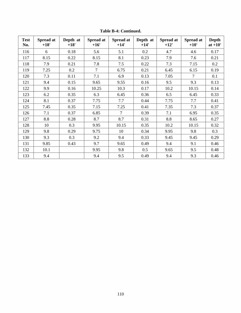
110
Table B-4: Continued.
Test
No.
Spread at
+18'
Depth at
+18'
Spread at
+16'
Spread at
+14'
Depth at
+14'
Spread at
+12'
Spread at
+10'
Depth
at +10'
116 6 0.18 5.6 5.1 0.2 4.7 4.6 0.17
117 8.15 0.22 8.15 8.1 0.23 7.9 7.6 0.21
118 7.9 0.21 7.8 7.5 0.22 7.3 7.15 0.2
119 7.25 0.2 7 6.75 0.21 6.45 6.15 0.19
120 7.3 0.11 7.1 6.9 0.13 7.05 7 0.1
121 9.4 0.15 9.65 9.55 0.16 9.5 9.3 0.13
122 9.9 0.16 10.25 10.3 0.17 10.2 10.15 0.14
123 6.2 0.35 6.3 6.45 0.36 6.5 6.45 0.33
124 8.1 0.37 7.75 7.7 0.44 7.75 7.7 0.41
125 7.45 0.35 7.15 7.25 0.41 7.35 7.3 0.37
126 7.1 0.37 6.85 7 0.39 7.1 6.95 0.35
127 8.8 0.28 8.7 8.7 0.31 8.8 8.65 0.27
128 10 0.3 9.95 10.15 0.35 10.2 10.15 0.32
129 9.8 0.29 9.75 10 0.34 9.95 9.8 0.3
130 9.3 0.3 9.2 9.4 0.33 9.45 9.45 0.29
131 9.85 0.43 9.7 9.65 0.49 9.4 9.1 0.46
132 10.1 9.95 9.8 0.5 9.65 9.5 0.48
133 9.4 9.4 9.5 0.49 9.4 9.3 0.46
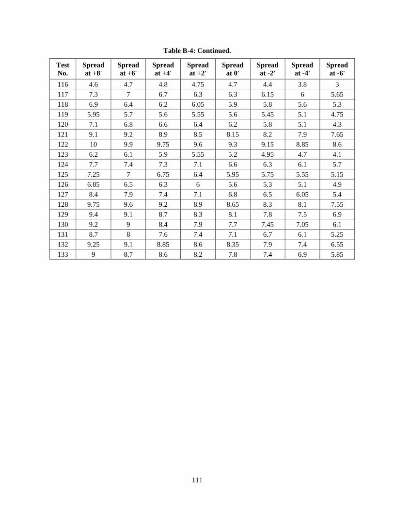
111
Table B-4: Continued.
Test
No.
Spread
at +8'
Spread
at +6'
Spread
at +4'
Spread
at +2'
Spread
at 0'
Spread
at -2'
Spread
at -4'
Spread
at -6'
116 4.6 4.7 4.8 4.75 4.7 4.4 3.8 3
117 7.3 7 6.7 6.3 6.3 6.15 6 5.65
118 6.9 6.4 6.2 6.05 5.9 5.8 5.6 5.3
119 5.95 5.7 5.6 5.55 5.6 5.45 5.1 4.75
120 7.1 6.8 6.6 6.4 6.2 5.8 5.1 4.3
121 9.1 9.2 8.9 8.5 8.15 8.2 7.9 7.65
122 10 9.9 9.75 9.6 9.3 9.15 8.85 8.6
123 6.2 6.1 5.9 5.55 5.2 4.95 4.7 4.1
124 7.7 7.4 7.3 7.1 6.6 6.3 6.1 5.7
125 7.25 7 6.75 6.4 5.95 5.75 5.55 5.15
126 6.85 6.5 6.3 6 5.6 5.3 5.1 4.9
127 8.4 7.9 7.4 7.1 6.8 6.5 6.05 5.4
128 9.75 9.6 9.2 8.9 8.65 8.3 8.1 7.55
129 9.4 9.1 8.7 8.3 8.1 7.8 7.5 6.9
130 9.2 9 8.4 7.9 7.7 7.45 7.05 6.1
131 8.7 8 7.6 7.4 7.1 6.7 6.1 5.25
132 9.25 9.1 8.85 8.6 8.35 7.9 7.4 6.55
133 9 8.7 8.6 8.2 7.8 7.4 6.9 5.85
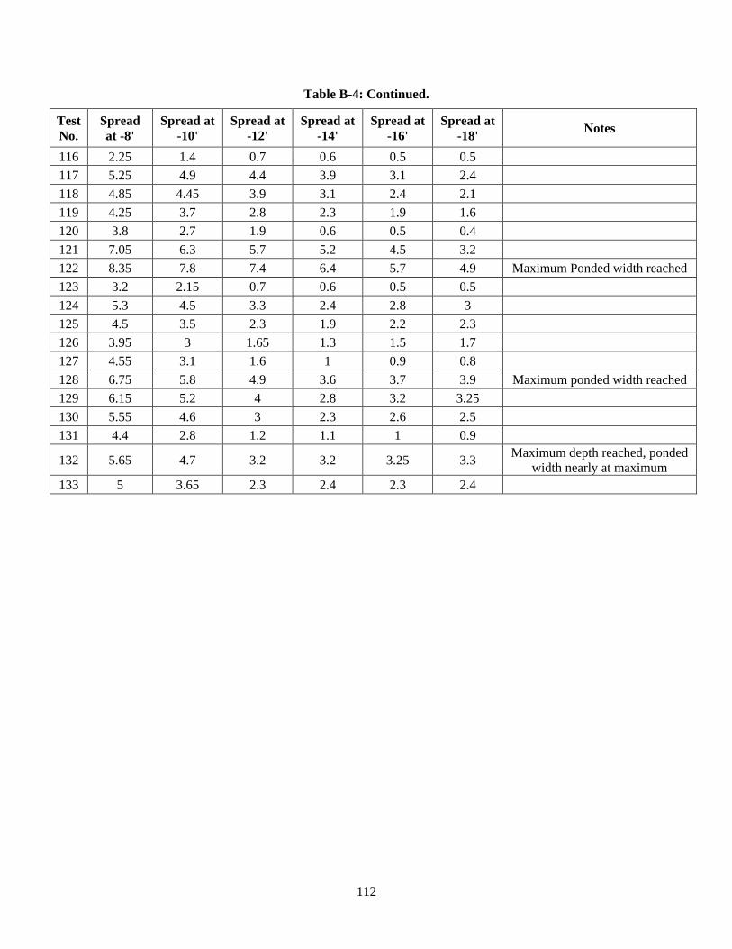
112
Table B-4: Continued.
Test
No.
Spread
at -8'
Spread at
-10'
Spread at
-12'
Spread at
-14'
Spread at
-16'
Spread at
-18' Notes
116 2.25 1.4 0.7 0.6 0.5 0.5
117 5.25 4.9 4.4 3.9 3.1 2.4
118 4.85 4.45 3.9 3.1 2.4 2.1
119 4.25 3.7 2.8 2.3 1.9 1.6
120 3.8 2.7 1.9 0.6 0.5 0.4
121 7.05 6.3 5.7 5.2 4.5 3.2
122 8.35 7.8 7.4 6.4 5.7 4.9 Maximum Ponded width reached
123 3.2 2.15 0.7 0.6 0.5 0.5
124 5.3 4.5 3.3 2.4 2.8 3
125 4.5 3.5 2.3 1.9 2.2 2.3
126 3.95 3 1.65 1.3 1.5 1.7
127 4.55 3.1 1.6 1 0.9 0.8
128 6.75 5.8 4.9 3.6 3.7 3.9 Maximum ponded width reached
129 6.15 5.2 4 2.8 3.2 3.25
130 5.55 4.6 3 2.3 2.6 2.5
131 4.4 2.8 1.2 1.1 1 0.9
132 5.65 4.7 3.2 3.2 3.25 3.3 Maximum depth reached, ponded
width nearly at maximum
133 5 3.65 2.3 2.4 2.3 2.4
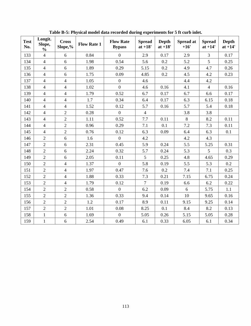
113
Table B-5: Physical model data recorded during experiments for 5 ft curb inlet.
Test
No.
Longit.
Slope,
%
Cross
Slope,% Flow Rate 1
Flow Rate
Bypass
Spread
at +18'
Depth
at +18'
Spread at
+16'
Spread
at +14'
Depth
at +14'
133 4 6 0.84 0 2.9 0.17 2.9 3 0.17
134 4 6 1.98 0.54 5.6 0.2 5.2 5 0.25
135 4 6 1.89 0.29 5.15 0.2 4.9 4.7 0.26
136 4 6 1.75 0.09 4.85 0.2 4.5 4.2 0.23
137 4 4 1.05 0 4.6 4.4 4.2
138 4 4 1.02 0 4.6 0.16 4.1 4 0.16
139 4 4 1.79 0.52 6.7 0.17 6.7 6.6 0.17
140 4 4 1.7 0.34 6.4 0.17 6.3 6.15 0.18
141 4 4 1.52 0.12 5.7 0.16 5.7 5.4 0.18
142 4 2 0.28 0 4 3.8 3.8
143 4 2 1.11 0.52 7.7 0.11 8 8.2 0.11
144 4 2 0.96 0.29 7.1 0.1 7.2 7.3 0.11
145 4 2 0.76 0.12 6.3 0.09 6.4 6.3 0.1
146 2 6 1.6 0 4.2 4.2 4.3
147 2 6 2.31 0.45 5.9 0.24 5.5 5.25 0.31
148 2 6 2.24 0.32 5.7 0.24 5.3 5 0.3
149 2 6 2.05 0.11 5 0.25 4.8 4.65 0.29
150 2 4 1.37 0 5.8 0.19 5.5 5.3 0.2
151 2 4 1.97 0.47 7.6 0.2 7.4 7.1 0.25
152 2 4 1.88 0.33 7.3 0.21 7.15 6.75 0.24
153 2 4 1.79 0.12 7 0.19 6.6 6.2 0.22
154 2 2 0.58 0 6.2 0.09 6 5.75 1.1
155 2 2 1.36 0.33 9.4 0.14 10 9.65 0.16
156 2 2 1.2 0.17 8.9 0.11 9.15 9.25 0.14
157 2 2 1.01 0.08 8.25 0.1 8.4 8.2 0.13
158 1 6 1.69 0 5.05 0.26 5.15 5.05 0.28
159 1 6 2.54 0.49 6.1 0.33 6.05 6.1 0.34
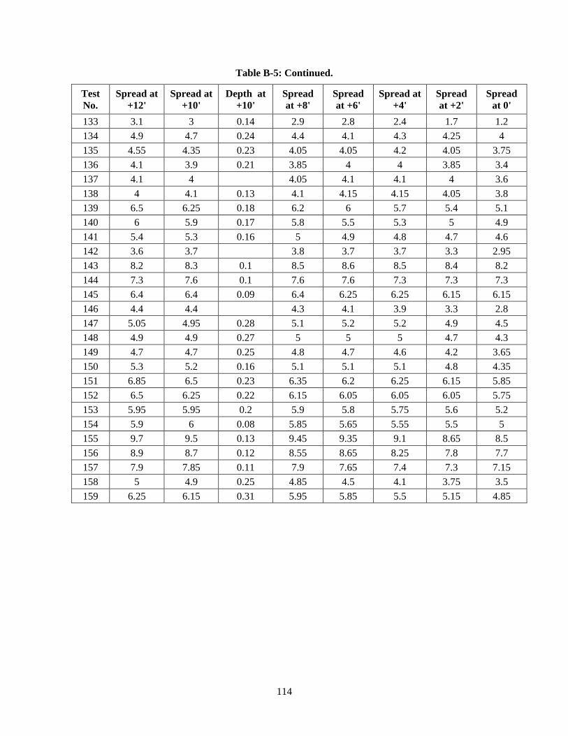
114
Table B-5: Continued.
Test
No.
Spread at
+12'
Spread at
+10'
Depth at
+10'
Spread
at +8'
Spread
at +6'
Spread at
+4'
Spread
at +2'
Spread
at 0'
133 3.1 3 0.14 2.9 2.8 2.4 1.7 1.2
134 4.9 4.7 0.24 4.4 4.1 4.3 4.25 4
135 4.55 4.35 0.23 4.05 4.05 4.2 4.05 3.75
136 4.1 3.9 0.21 3.85 4 4 3.85 3.4
137 4.1 4 4.05 4.1 4.1 4 3.6
138 4 4.1 0.13 4.1 4.15 4.15 4.05 3.8
139 6.5 6.25 0.18 6.2 6 5.7 5.4 5.1
140 6 5.9 0.17 5.8 5.5 5.3 5 4.9
141 5.4 5.3 0.16 5 4.9 4.8 4.7 4.6
142 3.6 3.7 3.8 3.7 3.7 3.3 2.95
143 8.2 8.3 0.1 8.5 8.6 8.5 8.4 8.2
144 7.3 7.6 0.1 7.6 7.6 7.3 7.3 7.3
145 6.4 6.4 0.09 6.4 6.25 6.25 6.15 6.15
146 4.4 4.4 4.3 4.1 3.9 3.3 2.8
147 5.05 4.95 0.28 5.1 5.2 5.2 4.9 4.5
148 4.9 4.9 0.27 5 5 5 4.7 4.3
149 4.7 4.7 0.25 4.8 4.7 4.6 4.2 3.65
150 5.3 5.2 0.16 5.1 5.1 5.1 4.8 4.35
151 6.85 6.5 0.23 6.35 6.2 6.25 6.15 5.85
152 6.5 6.25 0.22 6.15 6.05 6.05 6.05 5.75
153 5.95 5.95 0.2 5.9 5.8 5.75 5.6 5.2
154 5.9 6 0.08 5.85 5.65 5.55 5.5 5
155 9.7 9.5 0.13 9.45 9.35 9.1 8.65 8.5
156 8.9 8.7 0.12 8.55 8.65 8.25 7.8 7.7
157 7.9 7.85 0.11 7.9 7.65 7.4 7.3 7.15
158 5 4.9 0.25 4.85 4.5 4.1 3.75 3.5
159 6.25 6.15 0.31 5.95 5.85 5.5 5.15 4.85
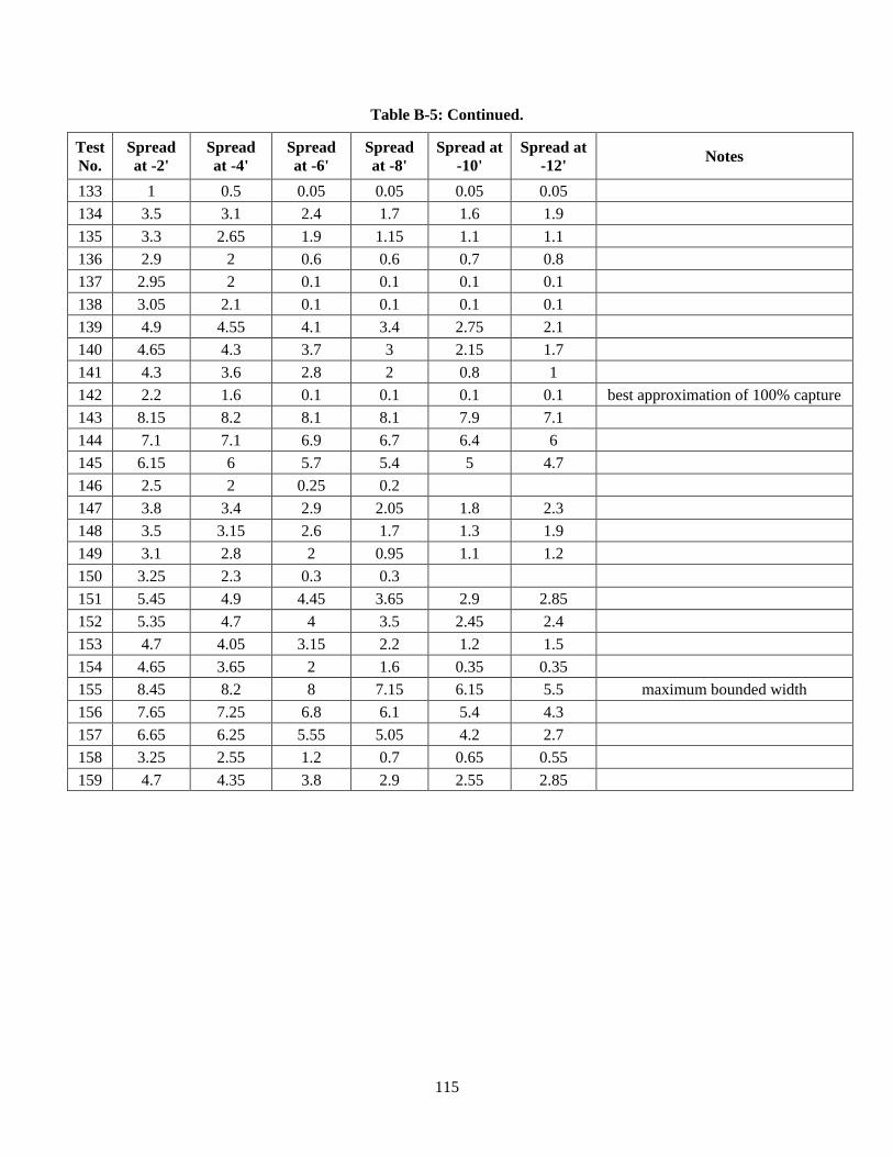
115
Table B-5: Continued.
Test
No.
Spread
at -2'
Spread
at -4'
Spread
at -6'
Spread
at -8'
Spread at
-10'
Spread at
-12' Notes
133 1 0.5 0.05 0.05 0.05 0.05
134 3.5 3.1 2.4 1.7 1.6 1.9
135 3.3 2.65 1.9 1.15 1.1 1.1
136 2.9 2 0.6 0.6 0.7 0.8
137 2.95 2 0.1 0.1 0.1 0.1
138 3.05 2.1 0.1 0.1 0.1 0.1
139 4.9 4.55 4.1 3.4 2.75 2.1
140 4.65 4.3 3.7 3 2.15 1.7
141 4.3 3.6 2.8 2 0.8 1
142 2.2 1.6 0.1 0.1 0.1 0.1 best approximation of 100% capture
143 8.15 8.2 8.1 8.1 7.9 7.1
144 7.1 7.1 6.9 6.7 6.4 6
145 6.15 6 5.7 5.4 5 4.7
146 2.5 2 0.25 0.2
147 3.8 3.4 2.9 2.05 1.8 2.3
148 3.5 3.15 2.6 1.7 1.3 1.9
149 3.1 2.8 2 0.95 1.1 1.2
150 3.25 2.3 0.3 0.3
151 5.45 4.9 4.45 3.65 2.9 2.85
152 5.35 4.7 4 3.5 2.45 2.4
153 4.7 4.05 3.15 2.2 1.2 1.5
154 4.65 3.65 2 1.6 0.35 0.35
155 8.45 8.2 8 7.15 6.15 5.5 maximum bounded width
156 7.65 7.25 6.8 6.1 5.4 4.3
157 6.65 6.25 5.55 5.05 4.2 2.7
158 3.25 2.55 1.2 0.7 0.65 0.55
159 4.7 4.35 3.8 2.9 2.55 2.85
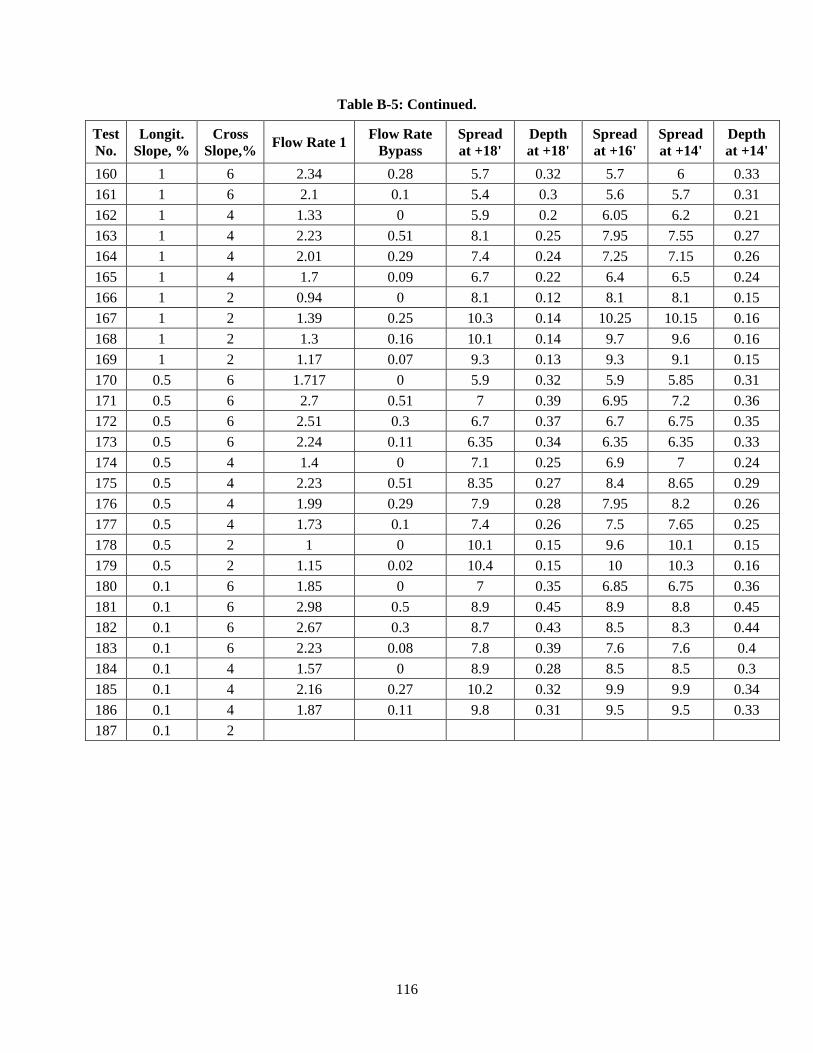
116
Table B-5: Continued.
Test
No.
Longit.
Slope, %
Cross
Slope,% Flow Rate 1
Flow Rate
Bypass
Spread
at +18'
Depth
at +18'
Spread
at +16'
Spread
at +14'
Depth
at +14'
160 1 6 2.34 0.28 5.7 0.32 5.7 6 0.33
161 1 6 2.1 0.1 5.4 0.3 5.6 5.7 0.31
162 1 4 1.33 0 5.9 0.2 6.05 6.2 0.21
163 1 4 2.23 0.51 8.1 0.25 7.95 7.55 0.27
164 1 4 2.01 0.29 7.4 0.24 7.25 7.15 0.26
165 1 4 1.7 0.09 6.7 0.22 6.4 6.5 0.24
166 1 2 0.94 0 8.1 0.12 8.1 8.1 0.15
167 1 2 1.39 0.25 10.3 0.14 10.25 10.15 0.16
168 1 2 1.3 0.16 10.1 0.14 9.7 9.6 0.16
169 1 2 1.17 0.07 9.3 0.13 9.3 9.1 0.15
170 0.5 6 1.717 0 5.9 0.32 5.9 5.85 0.31
171 0.5 6 2.7 0.51 7 0.39 6.95 7.2 0.36
172 0.5 6 2.51 0.3 6.7 0.37 6.7 6.75 0.35
173 0.5 6 2.24 0.11 6.35 0.34 6.35 6.35 0.33
174 0.5 4 1.4 0 7.1 0.25 6.9 7 0.24
175 0.5 4 2.23 0.51 8.35 0.27 8.4 8.65 0.29
176 0.5 4 1.99 0.29 7.9 0.28 7.95 8.2 0.26
177 0.5 4 1.73 0.1 7.4 0.26 7.5 7.65 0.25
178 0.5 2 1 0 10.1 0.15 9.6 10.1 0.15
179 0.5 2 1.15 0.02 10.4 0.15 10 10.3 0.16
180 0.1 6 1.85 0 7 0.35 6.85 6.75 0.36
181 0.1 6 2.98 0.5 8.9 0.45 8.9 8.8 0.45
182 0.1 6 2.67 0.3 8.7 0.43 8.5 8.3 0.44
183 0.1 6 2.23 0.08 7.8 0.39 7.6 7.6 0.4
184 0.1 4 1.57 0 8.9 0.28 8.5 8.5 0.3
185 0.1 4 2.16 0.27 10.2 0.32 9.9 9.9 0.34
186 0.1 4 1.87 0.11 9.8 0.31 9.5 9.5 0.33
187 0.1 2
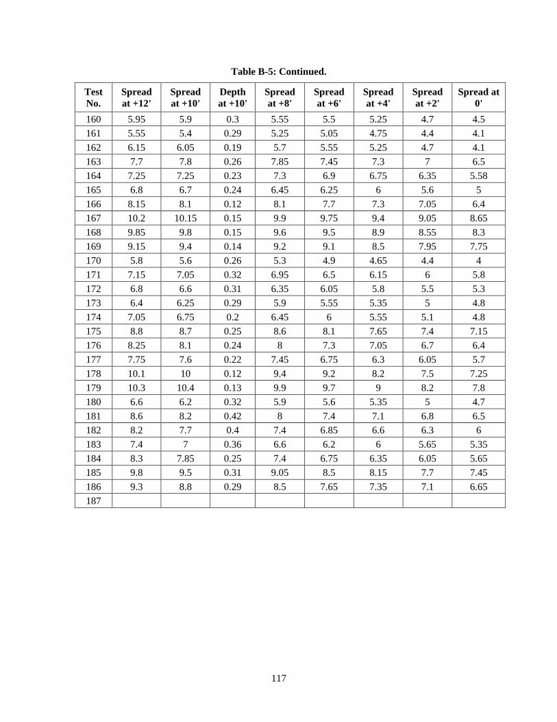
117
Table B-5: Continued.
Test
No.
Spread
at +12'
Spread
at +10'
Depth
at +10'
Spread
at +8'
Spread
at +6'
Spread
at +4'
Spread
at +2'
Spread at
0'
160 5.95 5.9 0.3 5.55 5.5 5.25 4.7 4.5
161 5.55 5.4 0.29 5.25 5.05 4.75 4.4 4.1
162 6.15 6.05 0.19 5.7 5.55 5.25 4.7 4.1
163 7.7 7.8 0.26 7.85 7.45 7.3 7 6.5
164 7.25 7.25 0.23 7.3 6.9 6.75 6.35 5.58
165 6.8 6.7 0.24 6.45 6.25 6 5.6 5
166 8.15 8.1 0.12 8.1 7.7 7.3 7.05 6.4
167 10.2 10.15 0.15 9.9 9.75 9.4 9.05 8.65
168 9.85 9.8 0.15 9.6 9.5 8.9 8.55 8.3
169 9.15 9.4 0.14 9.2 9.1 8.5 7.95 7.75
170 5.8 5.6 0.26 5.3 4.9 4.65 4.4 4
171 7.15 7.05 0.32 6.95 6.5 6.15 6 5.8
172 6.8 6.6 0.31 6.35 6.05 5.8 5.5 5.3
173 6.4 6.25 0.29 5.9 5.55 5.35 5 4.8
174 7.05 6.75 0.2 6.45 6 5.55 5.1 4.8
175 8.8 8.7 0.25 8.6 8.1 7.65 7.4 7.15
176 8.25 8.1 0.24 8 7.3 7.05 6.7 6.4
177 7.75 7.6 0.22 7.45 6.75 6.3 6.05 5.7
178 10.1 10 0.12 9.4 9.2 8.2 7.5 7.25
179 10.3 10.4 0.13 9.9 9.7 9 8.2 7.8
180 6.6 6.2 0.32 5.9 5.6 5.35 5 4.7
181 8.6 8.2 0.42 8 7.4 7.1 6.8 6.5
182 8.2 7.7 0.4 7.4 6.85 6.6 6.3 6
183 7.4 7 0.36 6.6 6.2 6 5.65 5.35
184 8.3 7.85 0.25 7.4 6.75 6.35 6.05 5.65
185 9.8 9.5 0.31 9.05 8.5 8.15 7.7 7.45
186 9.3 8.8 0.29 8.5 7.65 7.35 7.1 6.65
187
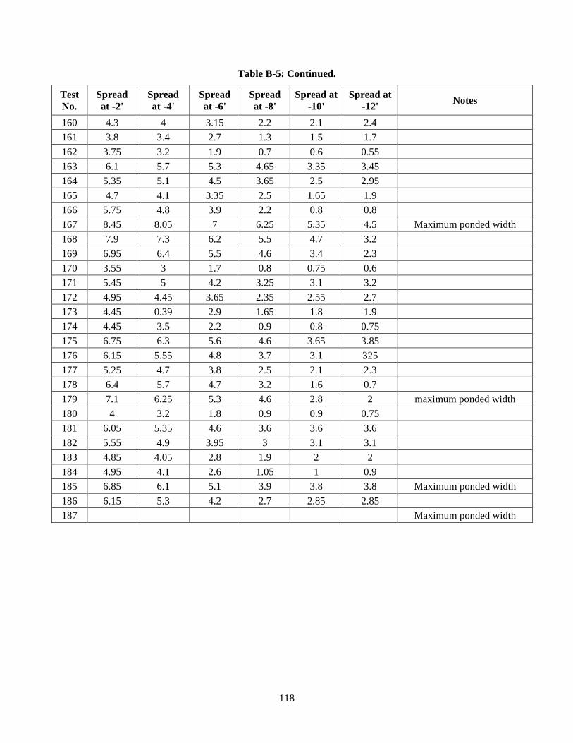
118
Table B-5: Continued.
Test
No.
Spread
at -2'
Spread
at -4'
Spread
at -6'
Spread
at -8'
Spread at
-10'
Spread at
-12' Notes
160 4.3 4 3.15 2.2 2.1 2.4
161 3.8 3.4 2.7 1.3 1.5 1.7
162 3.75 3.2 1.9 0.7 0.6 0.55
163 6.1 5.7 5.3 4.65 3.35 3.45
164 5.35 5.1 4.5 3.65 2.5 2.95
165 4.7 4.1 3.35 2.5 1.65 1.9
166 5.75 4.8 3.9 2.2 0.8 0.8
167 8.45 8.05 7 6.25 5.35 4.5 Maximum ponded width
168 7.9 7.3 6.2 5.5 4.7 3.2
169 6.95 6.4 5.5 4.6 3.4 2.3
170 3.55 3 1.7 0.8 0.75 0.6
171 5.45 5 4.2 3.25 3.1 3.2
172 4.95 4.45 3.65 2.35 2.55 2.7
173 4.45 0.39 2.9 1.65 1.8 1.9
174 4.45 3.5 2.2 0.9 0.8 0.75
175 6.75 6.3 5.6 4.6 3.65 3.85
176 6.15 5.55 4.8 3.7 3.1 325
177 5.25 4.7 3.8 2.5 2.1 2.3
178 6.4 5.7 4.7 3.2 1.6 0.7
179 7.1 6.25 5.3 4.6 2.8 2 maximum ponded width
180 4 3.2 1.8 0.9 0.9 0.75
181 6.05 5.35 4.6 3.6 3.6 3.6
182 5.55 4.9 3.95 3 3.1 3.1
183 4.85 4.05 2.8 1.9 2 2
184 4.95 4.1 2.6 1.05 1 0.9
185 6.85 6.1 5.1 3.9 3.8 3.8 Maximum ponded width
186 6.15 5.3 4.2 2.7 2.85 2.85
187 Maximum ponded width
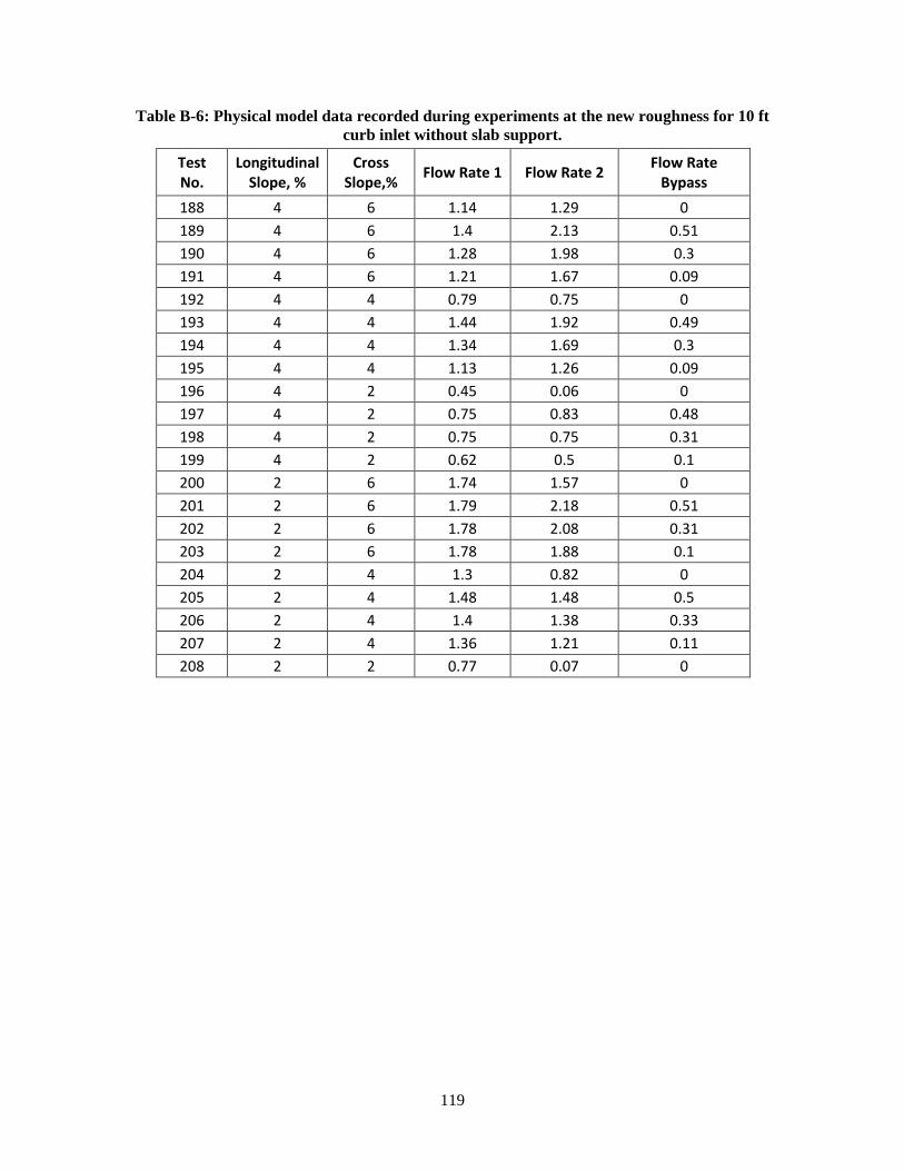
119
Table B-6: Physical model data recorded during experiments at the new roughness for 10 ft
curb inlet without slab support.
Test No.
Longitudinal Slope, %
Cross Slope,%
Flow Rate 1 Flow Rate 2 Flow Rate
Bypass
188 4 6 1.14 1.29 0
189 4 6 1.4 2.13 0.51
190 4 6 1.28 1.98 0.3
191 4 6 1.21 1.67 0.09
192 4 4 0.79 0.75 0
193 4 4 1.44 1.92 0.49
194 4 4 1.34 1.69 0.3
195 4 4 1.13 1.26 0.09
196 4 2 0.45 0.06 0
197 4 2 0.75 0.83 0.48
198 4 2 0.75 0.75 0.31
199 4 2 0.62 0.5 0.1
200 2 6 1.74 1.57 0
201 2 6 1.79 2.18 0.51
202 2 6 1.78 2.08 0.31
203 2 6 1.78 1.88 0.1
204 2 4 1.3 0.82 0
205 2 4 1.48 1.48 0.5
206 2 4 1.4 1.38 0.33
207 2 4 1.36 1.21 0.11
208 2 2 0.77 0.07 0
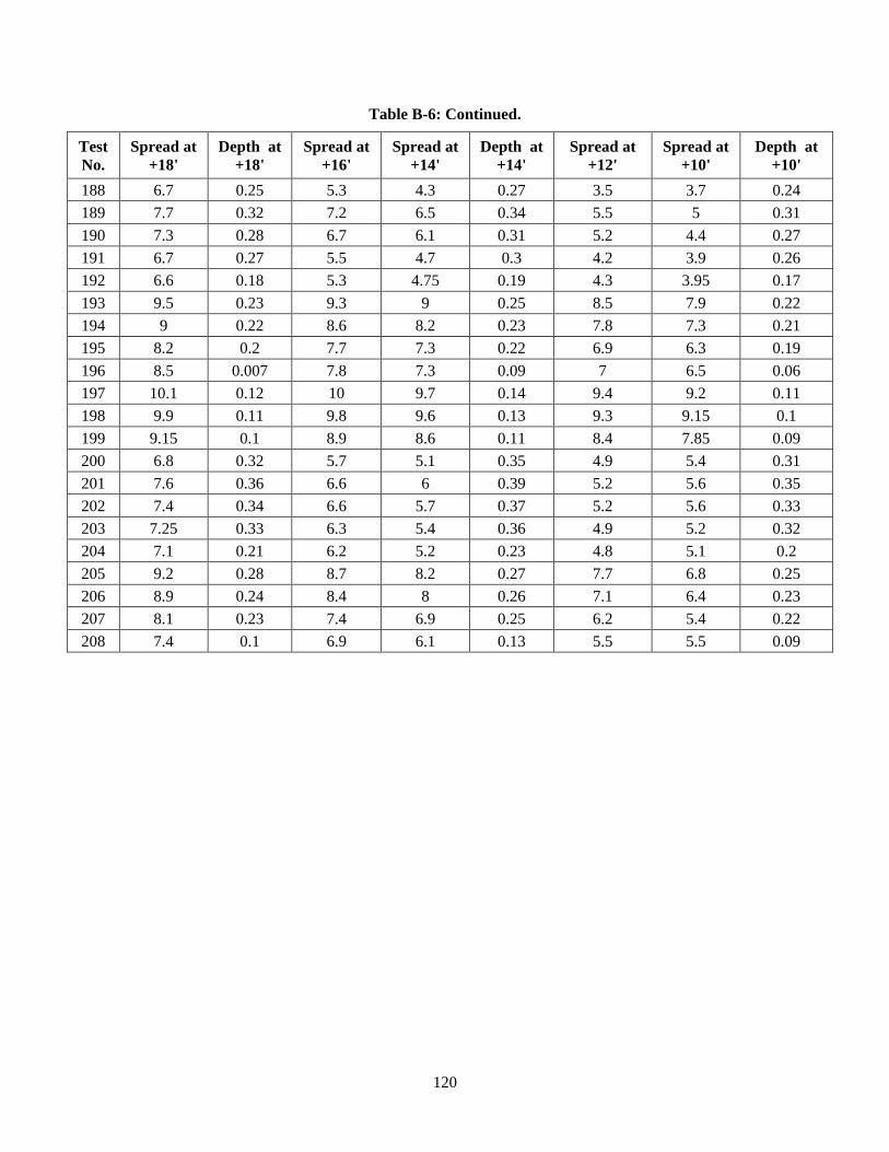
120
Table B-6: Continued.
Test
No.
Spread at
+18'
Depth at
+18'
Spread at
+16'
Spread at
+14'
Depth at
+14'
Spread at
+12'
Spread at
+10'
Depth at
+10'
188 6.7 0.25 5.3 4.3 0.27 3.5 3.7 0.24
189 7.7 0.32 7.2 6.5 0.34 5.5 5 0.31
190 7.3 0.28 6.7 6.1 0.31 5.2 4.4 0.27
191 6.7 0.27 5.5 4.7 0.3 4.2 3.9 0.26
192 6.6 0.18 5.3 4.75 0.19 4.3 3.95 0.17
193 9.5 0.23 9.3 9 0.25 8.5 7.9 0.22
194 9 0.22 8.6 8.2 0.23 7.8 7.3 0.21
195 8.2 0.2 7.7 7.3 0.22 6.9 6.3 0.19
196 8.5 0.007 7.8 7.3 0.09 7 6.5 0.06
197 10.1 0.12 10 9.7 0.14 9.4 9.2 0.11
198 9.9 0.11 9.8 9.6 0.13 9.3 9.15 0.1
199 9.15 0.1 8.9 8.6 0.11 8.4 7.85 0.09
200 6.8 0.32 5.7 5.1 0.35 4.9 5.4 0.31
201 7.6 0.36 6.6 6 0.39 5.2 5.6 0.35
202 7.4 0.34 6.6 5.7 0.37 5.2 5.6 0.33
203 7.25 0.33 6.3 5.4 0.36 4.9 5.2 0.32
204 7.1 0.21 6.2 5.2 0.23 4.8 5.1 0.2
205 9.2 0.28 8.7 8.2 0.27 7.7 6.8 0.25
206 8.9 0.24 8.4 8 0.26 7.1 6.4 0.23
207 8.1 0.23 7.4 6.9 0.25 6.2 5.4 0.22
208 7.4 0.1 6.9 6.1 0.13 5.5 5.5 0.09
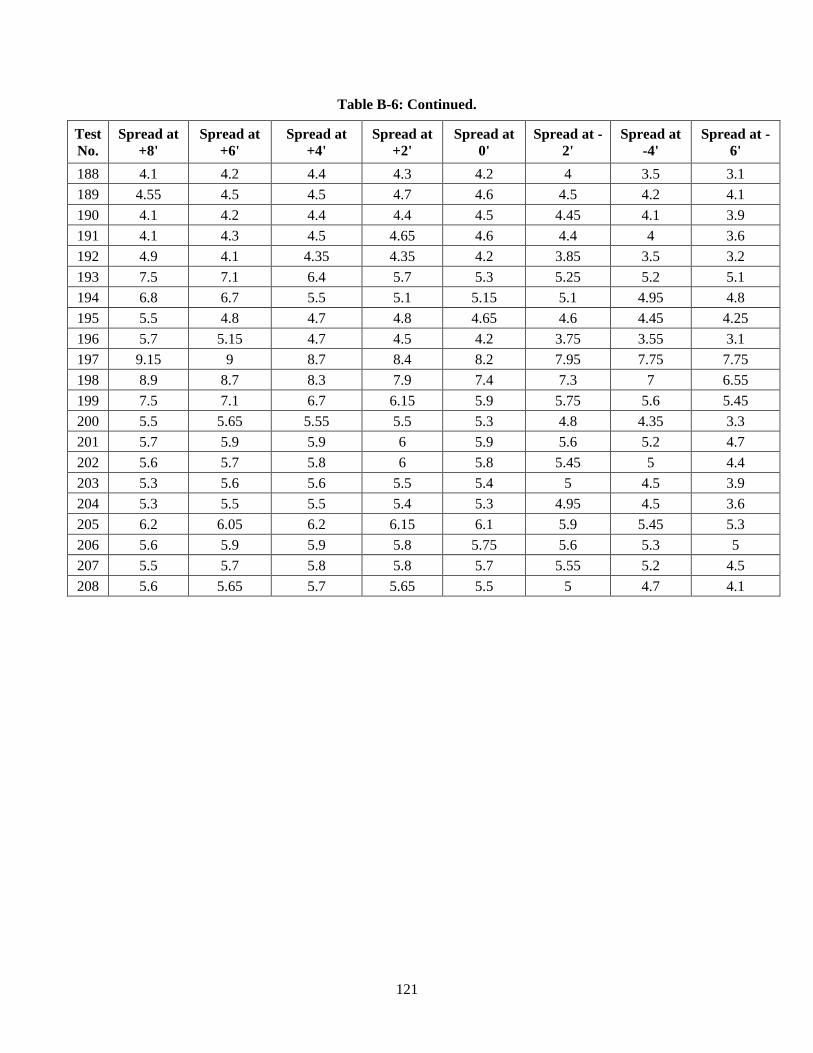
121
Table B-6: Continued.
Test
No.
Spread at
+8'
Spread at
+6'
Spread at
+4'
Spread at
+2'
Spread at
0'
Spread at -
2'
Spread at
-4'
Spread at -
6'
188 4.1 4.2 4.4 4.3 4.2 4 3.5 3.1
189 4.55 4.5 4.5 4.7 4.6 4.5 4.2 4.1
190 4.1 4.2 4.4 4.4 4.5 4.45 4.1 3.9
191 4.1 4.3 4.5 4.65 4.6 4.4 4 3.6
192 4.9 4.1 4.35 4.35 4.2 3.85 3.5 3.2
193 7.5 7.1 6.4 5.7 5.3 5.25 5.2 5.1
194 6.8 6.7 5.5 5.1 5.15 5.1 4.95 4.8
195 5.5 4.8 4.7 4.8 4.65 4.6 4.45 4.25
196 5.7 5.15 4.7 4.5 4.2 3.75 3.55 3.1
197 9.15 9 8.7 8.4 8.2 7.95 7.75 7.75
198 8.9 8.7 8.3 7.9 7.4 7.3 7 6.55
199 7.5 7.1 6.7 6.15 5.9 5.75 5.6 5.45
200 5.5 5.65 5.55 5.5 5.3 4.8 4.35 3.3
201 5.7 5.9 5.9 6 5.9 5.6 5.2 4.7
202 5.6 5.7 5.8 6 5.8 5.45 5 4.4
203 5.3 5.6 5.6 5.5 5.4 5 4.5 3.9
204 5.3 5.5 5.5 5.4 5.3 4.95 4.5 3.6
205 6.2 6.05 6.2 6.15 6.1 5.9 5.45 5.3
206 5.6 5.9 5.9 5.8 5.75 5.6 5.3 5
207 5.5 5.7 5.8 5.8 5.7 5.55 5.2 4.5
208 5.6 5.65 5.7 5.65 5.5 5 4.7 4.1
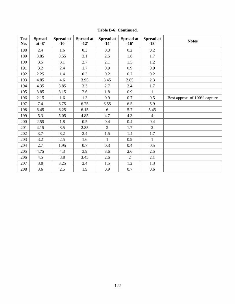
122
Table B-6: Continued.
Test
No.
Spread
at -8'
Spread at
-10'
Spread at
-12'
Spread at
-14'
Spread at
-16'
Spread at
-18' Notes
188 2.4 1.6 0.3 0.3 0.2 0.2
189 3.85 3.55 3.1 2.5 1.8 1.7
190 3.5 3.1 2.7 2.1 1.5 1.2
191 3.2 2.4 1.7 0.9 0.9 0.9
192 2.25 1.4 0.3 0.2 0.2 0.2
193 4.85 4.6 3.95 3.45 2.85 2.3
194 4.35 3.85 3.3 2.7 2.4 1.7
195 3.85 3.15 2.6 1.8 0.9 1
196 2.15 1.6 1.3 0.9 0.7 0.5 Best approx. of 100% capture
197 7.4 6.75 6.75 6.55 6.5 5.9
198 6.45 6.25 6.15 6 5.7 5.45
199 5.3 5.05 4.85 4.7 4.3 4
200 2.55 1.8 0.5 0.4 0.4 0.4
201 4.15 3.5 2.85 2 1.7 2
202 3.7 3.2 2.4 1.5 1.4 1.7
203 3.2 2.5 1.6 1 0.9 1
204 2.7 1.95 0.7 0.3 0.4 0.5
205 4.75 4.3 3.9 3.6 2.6 2.5
206 4.5 3.8 3.45 2.6 2 2.1
207 3.8 3.25 2.4 1.5 1.2 1.3
208 3.6 2.5 1.9 0.9 0.7 0.6
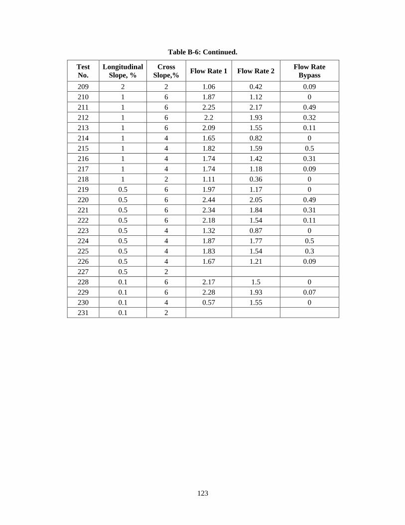
123
Table B-6: Continued.
Test
No.
Longitudinal
Slope, %
Cross
Slope,% Flow Rate 1 Flow Rate 2
Flow Rate
Bypass
209 2 2 1.06 0.42 0.09
210 1 6 1.87 1.12 0
211 1 6 2.25 2.17 0.49
212 1 6 2.2 1.93 0.32
213 1 6 2.09 1.55 0.11
214 1 4 1.65 0.82 0
215 1 4 1.82 1.59 0.5
216 1 4 1.74 1.42 0.31
217 1 4 1.74 1.18 0.09
218 1 2 1.11 0.36 0
219 0.5 6 1.97 1.17 0
220 0.5 6 2.44 2.05 0.49
221 0.5 6 2.34 1.84 0.31
222 0.5 6 2.18 1.54 0.11
223 0.5 4 1.32 0.87 0
224 0.5 4 1.87 1.77 0.5
225 0.5 4 1.83 1.54 0.3
226 0.5 4 1.67 1.21 0.09
227 0.5 2
228 0.1 6 2.17 1.5 0
229 0.1 6 2.28 1.93 0.07
230 0.1 4 0.57 1.55 0
231 0.1 2
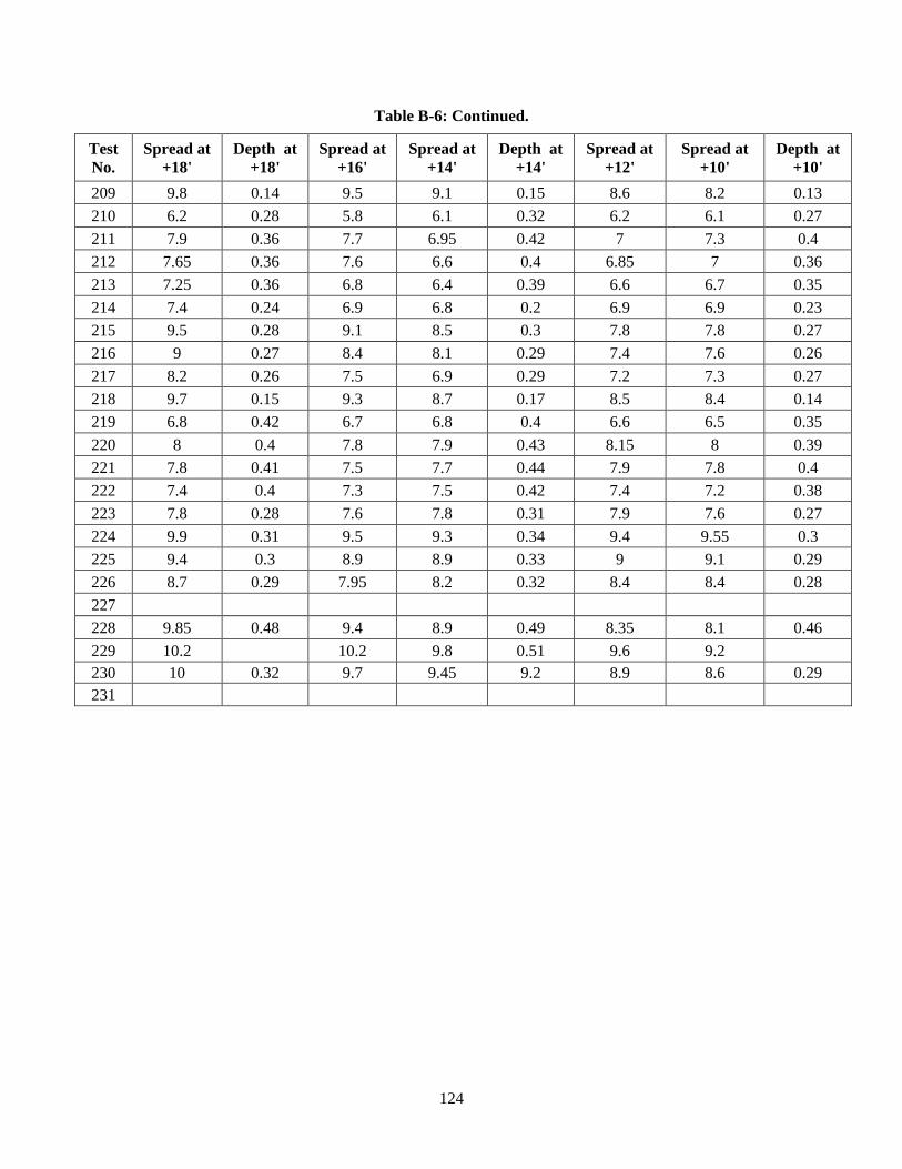
124
Table B-6: Continued.
Test
No.
Spread at
+18'
Depth at
+18'
Spread at
+16'
Spread at
+14'
Depth at
+14'
Spread at
+12'
Spread at
+10'
Depth at
+10'
209 9.8 0.14 9.5 9.1 0.15 8.6 8.2 0.13
210 6.2 0.28 5.8 6.1 0.32 6.2 6.1 0.27
211 7.9 0.36 7.7 6.95 0.42 7 7.3 0.4
212 7.65 0.36 7.6 6.6 0.4 6.85 7 0.36
213 7.25 0.36 6.8 6.4 0.39 6.6 6.7 0.35
214 7.4 0.24 6.9 6.8 0.2 6.9 6.9 0.23
215 9.5 0.28 9.1 8.5 0.3 7.8 7.8 0.27
216 9 0.27 8.4 8.1 0.29 7.4 7.6 0.26
217 8.2 0.26 7.5 6.9 0.29 7.2 7.3 0.27
218 9.7 0.15 9.3 8.7 0.17 8.5 8.4 0.14
219 6.8 0.42 6.7 6.8 0.4 6.6 6.5 0.35
220 8 0.4 7.8 7.9 0.43 8.15 8 0.39
221 7.8 0.41 7.5 7.7 0.44 7.9 7.8 0.4
222 7.4 0.4 7.3 7.5 0.42 7.4 7.2 0.38
223 7.8 0.28 7.6 7.8 0.31 7.9 7.6 0.27
224 9.9 0.31 9.5 9.3 0.34 9.4 9.55 0.3
225 9.4 0.3 8.9 8.9 0.33 9 9.1 0.29
226 8.7 0.29 7.95 8.2 0.32 8.4 8.4 0.28
227
228 9.85 0.48 9.4 8.9 0.49 8.35 8.1 0.46
229 10.2 10.2 9.8 0.51 9.6 9.2
230 10 0.32 9.7 9.45 9.2 8.9 8.6 0.29
231
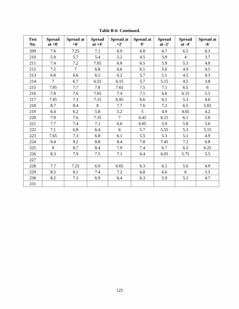
125
Table B-6: Continued.
Test
No.
Spread
at +8'
Spread at
+6'
Spread
at +4'
Spread at
+2'
Spread at
0'
Spread
at -2'
Spread
at -4'
Spread at
-6'
209 7.6 7.25 7.1 6.9 6.8 6.7 6.5 6.3
210 5.9 5.7 5.4 5.2 4.5 3.9 4 3.7
211 7.4 7.2 7.05 6.8 6.5 5.9 5.3 4.8
212 7.2 7 6.8 6.6 6.1 5.6 4.9 4.5
213 6.8 6.6 6.5 6.2 5.7 5.1 4.5 4.3
214 7 6.7 6.55 6.15 5.7 5.15 4.5 3.8
215 7.95 7.7 7.8 7.65 7.5 7.1 6.5 6
216 7.8 7.6 7.65 7.4 7.1 6.6 6.15 5.5
217 7.45 7.3 7.15 6.95 6.6 6.1 5.3 4.6
218 8.7 8.4 8 7.7 7.6 7.2 6.5 5.65
219 6.4 6.2 5.8 5.2 5 4.9 4.65 4.2
220 7.9 7.6 7.35 7 6.45 6.15 6.1 5.8
221 7.7 7.4 7.1 6.6 6.05 5.9 5.8 5.6
222 7.1 6.8 6.4 6 5.7 5.55 5.3 5.15
223 7.65 7.3 6.8 6.1 5.5 5.3 5.1 4.9
224 9.4 9.2 8.8 8.4 7.8 7.45 7.2 6.8
225 9 8.7 8.4 7.9 7.4 6.7 6.5 6.25
226 8.3 7.9 7.5 7.1 6.4 6.05 5.75 5.5
227
228 7.7 7.25 6.9 6.65 6.3 6.1 5.6 4.9
229 8.5 8.1 7.4 7.2 6.8 6.6 6 5.5
230 8.2 7.3 6.9 6.4 6.3 5.9 5.1 4.7
231
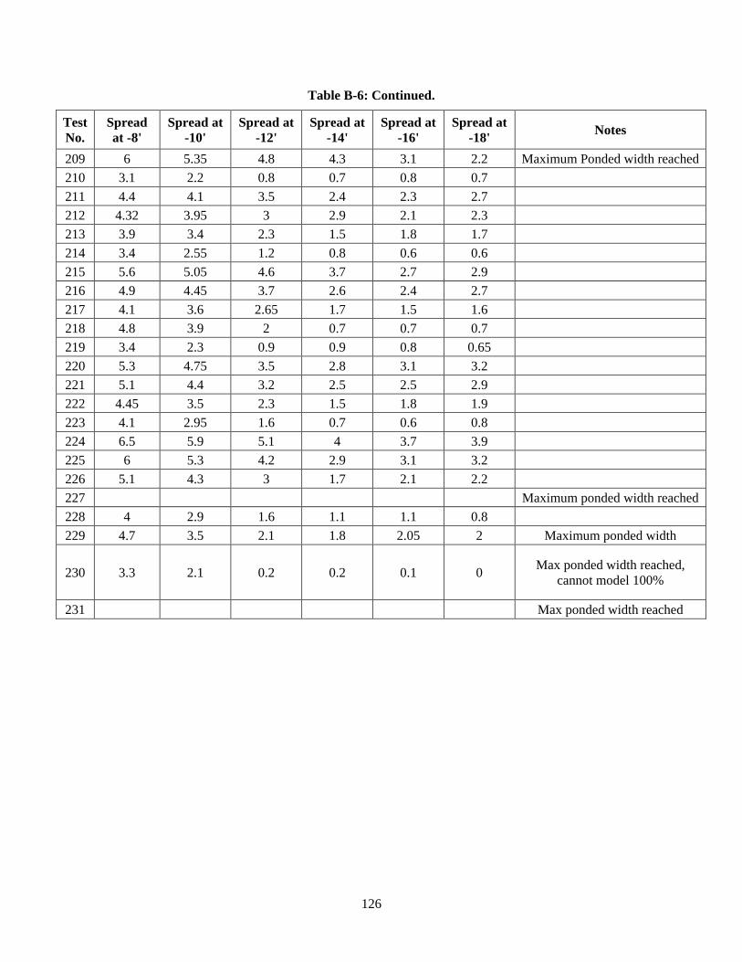
126
Table B-6: Continued.
Test
No.
Spread
at -8'
Spread at
-10'
Spread at
-12'
Spread at
-14'
Spread at
-16'
Spread at
-18' Notes
209 6 5.35 4.8 4.3 3.1 2.2 Maximum Ponded width reached
210 3.1 2.2 0.8 0.7 0.8 0.7
211 4.4 4.1 3.5 2.4 2.3 2.7
212 4.32 3.95 3 2.9 2.1 2.3
213 3.9 3.4 2.3 1.5 1.8 1.7
214 3.4 2.55 1.2 0.8 0.6 0.6
215 5.6 5.05 4.6 3.7 2.7 2.9
216 4.9 4.45 3.7 2.6 2.4 2.7
217 4.1 3.6 2.65 1.7 1.5 1.6
218 4.8 3.9 2 0.7 0.7 0.7
219 3.4 2.3 0.9 0.9 0.8 0.65
220 5.3 4.75 3.5 2.8 3.1 3.2
221 5.1 4.4 3.2 2.5 2.5 2.9
222 4.45 3.5 2.3 1.5 1.8 1.9
223 4.1 2.95 1.6 0.7 0.6 0.8
224 6.5 5.9 5.1 4 3.7 3.9
225 6 5.3 4.2 2.9 3.1 3.2
226 5.1 4.3 3 1.7 2.1 2.2
227 Maximum ponded width reached
228 4 2.9 1.6 1.1 1.1 0.8
229 4.7 3.5 2.1 1.8 2.05 2 Maximum ponded width
230 3.3 2.1 0.2 0.2 0.1 0 Max ponded width reached,
cannot model 100%
231 Max ponded width reached
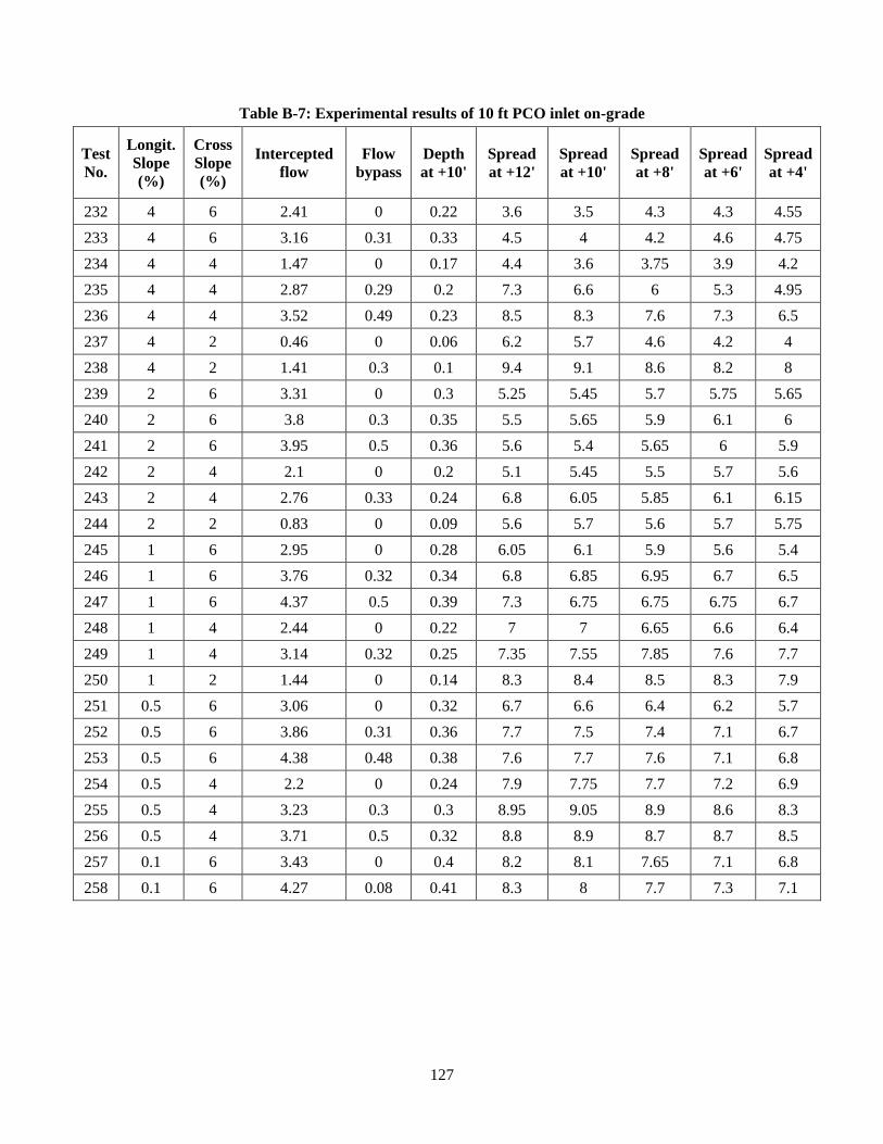
127
Table B-7: Experimental results of 10 ft PCO inlet on-grade
Test
No.
Longit.
Slope
(%)
Cross
Slope
(%)
Intercepted
flow
Flow
bypass
Depth
at +10'
Spread
at +12'
Spread
at +10'
Spread
at +8'
Spread
at +6'
Spread
at +4'
232 4 6 2.41 0 0.22 3.6 3.5 4.3 4.3 4.55
233 4 6 3.16 0.31 0.33 4.5 4 4.2 4.6 4.75
234 4 4 1.47 0 0.17 4.4 3.6 3.75 3.9 4.2
235 4 4 2.87 0.29 0.2 7.3 6.6 6 5.3 4.95
236 4 4 3.52 0.49 0.23 8.5 8.3 7.6 7.3 6.5
237 4 2 0.46 0 0.06 6.2 5.7 4.6 4.2 4
238 4 2 1.41 0.3 0.1 9.4 9.1 8.6 8.2 8
239 2 6 3.31 0 0.3 5.25 5.45 5.7 5.75 5.65
240 2 6 3.8 0.3 0.35 5.5 5.65 5.9 6.1 6
241 2 6 3.95 0.5 0.36 5.6 5.4 5.65 6 5.9
242 2 4 2.1 0 0.2 5.1 5.45 5.5 5.7 5.6
243 2 4 2.76 0.33 0.24 6.8 6.05 5.85 6.1 6.15
244 2 2 0.83 0 0.09 5.6 5.7 5.6 5.7 5.75
245 1 6 2.95 0 0.28 6.05 6.1 5.9 5.6 5.4
246 1 6 3.76 0.32 0.34 6.8 6.85 6.95 6.7 6.5
247 1 6 4.37 0.5 0.39 7.3 6.75 6.75 6.75 6.7
248 1 4 2.44 0 0.22 7 7 6.65 6.6 6.4
249 1 4 3.14 0.32 0.25 7.35 7.55 7.85 7.6 7.7
250 1 2 1.44 0 0.14 8.3 8.4 8.5 8.3 7.9
251 0.5 6 3.06 0 0.32 6.7 6.6 6.4 6.2 5.7
252 0.5 6 3.86 0.31 0.36 7.7 7.5 7.4 7.1 6.7
253 0.5 6 4.38 0.48 0.38 7.6 7.7 7.6 7.1 6.8
254 0.5 4 2.2 0 0.24 7.9 7.75 7.7 7.2 6.9
255 0.5 4 3.23 0.3 0.3 8.95 9.05 8.9 8.6 8.3
256 0.5 4 3.71 0.5 0.32 8.8 8.9 8.7 8.7 8.5
257 0.1 6 3.43 0 0.4 8.2 8.1 7.65 7.1 6.8
258 0.1 6 4.27 0.08 0.41 8.3 8 7.7 7.3 7.1
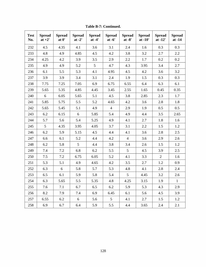
128
Table B-7: Continued.
Test
No.
Spread
at +2'
Spread
at 0'
Spread
at -2'
Spread
at -4'
Spread
at -6'
Spread
at -8'
Spread
at -10'
Spread
at -12'
Spread
at -14
232 4.5 4.35 4.1 3.6 3.1 2.4 1.6 0.3 0.3
233 4.8 4.9 4.85 4.5 4.2 3.8 3.2 2.7 2.2
234 4.25 4.2 3.9 3.5 2.9 2.2 1.7 0.2 0.2
235 4.9 4.9 5.2 5 4.7 4.3 3.95 3.4 2.7
236 6.1 5.5 5.3 4.1 4.95 4.5 4.2 3.6 3.2
237 3.9 3.9 3.4 3.1 2.4 1.9 1.5 0.3 0.3
238 7.75 7.25 7.05 6.9 6.75 6.55 6.4 6.3 6.1
239 5.65 5.35 4.85 4.45 3.45 2.55 1.65 0.45 0.35
240 6 6.05 5.65 5.1 4.5 3.8 2.85 2.3 1.7
241 5.85 5.75 5.5 5.2 4.65 4.2 3.6 2.8 1.8
242 5.65 5.45 5.1 4.9 4 2.9 1.9 0.5 0.5
243 6.2 6.15 6 5.85 5.4 4.9 4.4 3.5 2.65
244 5.7 5.6 5.4 5.25 4.9 4.1 2.7 1.8 1.6
245 5 4.35 3.95 4.05 3.7 3.1 2.2 1.5 1.2
246 6.2 5.9 5.15 4.5 4.4 4.1 3.6 2.8 2.5
247 6.6 6.1 5.2 4.4 4.2 4 3.6 2.9 2.6
248 6.2 5.8 5 4.4 3.8 3.4 2.6 1.5 1.2
249 7.4 7.2 6.8 6.2 5.5 5 4.5 3.9 2.5
250 7.5 7.2 6.75 6.05 5.2 4.1 3.3 2 1.6
251 5.3 5.1 4.9 4.65 4.2 3.5 2.7 1.2 0.9
252 6.3 6 5.8 5.7 5.3 4.8 4.1 2.8 2.4
253 6.5 6.1 5.9 5.8 5.4 5 4.45 3.2 2.6
254 6.3 5.65 5.5 5.35 4.8 4.25 3.15 1.9 1
255 7.6 7.1 6.7 6.5 6.2 5.9 5.3 4.3 2.9
256 8.2 7.9 7.4 6.9 6.45 6.1 5.6 4.5 3.9
257 6.55 6.2 6 5.6 5 4.1 2.7 1.5 1.2
258 6.9 6.7 6.4 5.9 5.5 4.4 3.65 2.4 2.1
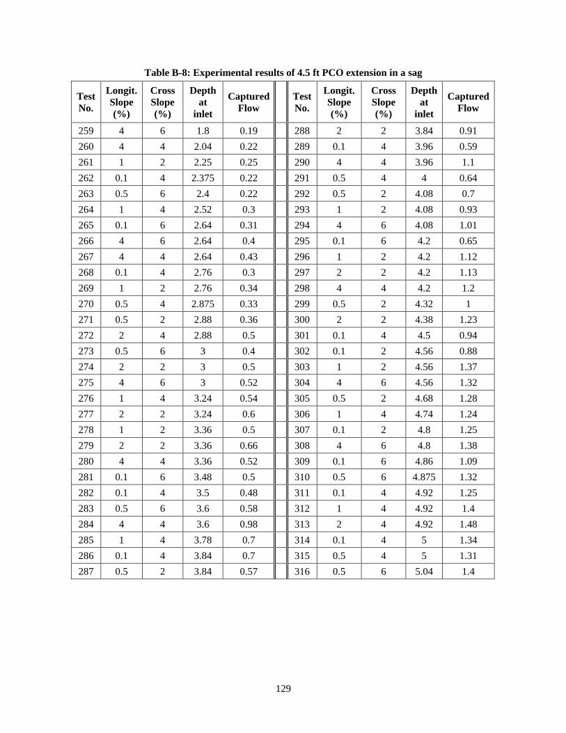
129
Table B-8: Experimental results of 4.5 ft PCO extension in a sag
Test
No.
Longit.
Slope
(%)
Cross
Slope
(%)
Depth
at
inlet
Captured
Flow
Test
No.
Longit.
Slope
(%)
Cross
Slope
(%)
Depth
at
inlet
Captured
Flow
259 4 6 1.8 0.19 288 2 2 3.84 0.91
260 4 4 2.04 0.22 289 0.1 4 3.96 0.59
261 1 2 2.25 0.25 290 4 4 3.96 1.1
262 0.1 4 2.375 0.22 291 0.5 4 4 0.64
263 0.5 6 2.4 0.22 292 0.5 2 4.08 0.7
264 1 4 2.52 0.3 293 1 2 4.08 0.93
265 0.1 6 2.64 0.31 294 4 6 4.08 1.01
266 4 6 2.64 0.4 295 0.1 6 4.2 0.65
267 4 4 2.64 0.43 296 1 2 4.2 1.12
268 0.1 4 2.76 0.3 297 2 2 4.2 1.13
269 1 2 2.76 0.34 298 4 4 4.2 1.2
270 0.5 4 2.875 0.33 299 0.5 2 4.32 1
271 0.5 2 2.88 0.36 300 2 2 4.38 1.23
272 2 4 2.88 0.5 301 0.1 4 4.5 0.94
273 0.5 6 3 0.4 302 0.1 2 4.56 0.88
274 2 2 3 0.5 303 1 2 4.56 1.37
275 4 6 3 0.52 304 4 6 4.56 1.32
276 1 4 3.24 0.54 305 0.5 2 4.68 1.28
277 2 2 3.24 0.6 306 1 4 4.74 1.24
278 1 2 3.36 0.5 307 0.1 2 4.8 1.25
279 2 2 3.36 0.66 308 4 6 4.8 1.38
280 4 4 3.36 0.52 309 0.1 6 4.86 1.09
281 0.1 6 3.48 0.5 310 0.5 6 4.875 1.32
282 0.1 4 3.5 0.48 311 0.1 4 4.92 1.25
283 0.5 6 3.6 0.58 312 1 4 4.92 1.4
284 4 4 3.6 0.98 313 2 4 4.92 1.48
285 1 4 3.78 0.7 314 0.1 4 5 1.34
286 0.1 4 3.84 0.7 315 0.5 4 5 1.31
287 0.5 2 3.84 0.57 316 0.5 6 5.04 1.4
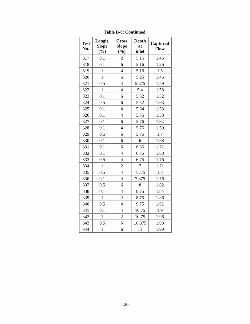
130
Table B-8: Continued.
Test
No.
Longit.
Slope
(%)
Cross
Slope
(%)
Depth
at
inlet
Captured
Flow
317 0.1 2 5.16 1.45
318 0.1 6 5.16 1.26
319 1 4 5.16 1.5
320 1 6 5.25 1.46
321 0.5 4 5.375 1.59
322 1 4 5.4 1.58
323 0.1 6 5.52 1.52
324 0.5 6 5.52 1.63
325 0.1 4 5.64 1.58
326 0.1 4 5.75 1.58
327 0.1 6 5.76 1.64
328 0.1 4 5.76 1.59
329 0.5 6 5.76 1.7
330 0.1 6 6 1.68
331 0.1 6 6.36 1.71
332 0.1 4 6.75 1.68
333 0.5 4 6.75 1.76
334 1 2 7 1.71
335 0.5 4 7.375 1.8
336 0.1 4 7.875 1.76
337 0.5 6 8 1.82
338 0.1 4 8.75 1.84
339 1 2 8.75 1.86
340 0.5 4 9.75 1.91
341 0.1 4 10.75 1.9
342 1 2 10.75 1.96
343 0.5 6 10.875 1.98
344 1 6 11 1.99