intercomparison of rain gauge, radar, and satellite-based...

Intercomparison of Rain Gauge, Radar, and Satellite-Based Precipitation Estimateswith Emphasis on Hydrologic Forecasting

KORAY K. YILMAZ

Department of Hydrology and Water Resources, The University of Arizona, Tucson, Arizona

TERRI S. HOGUE

Department of Civil and Environmental Engineering, University of California, Los Angeles, Los Angeles, California

KUO-LIN HSU AND SOROOSH SOROOSHIAN

Department of Civil and Environmental Engineering, University of California, Irvine, Irvine, California

HOSHIN V. GUPTA

Department of Hydrology and Water Resources, The University of Arizona, Tucson, Arizona

THORSTEN WAGENER

Department of Civil and Environmental Engineering, The Pennsylvania State University, University Park, Pennsylvania

(Manuscript received 14 October 2004, in final form 7 February 2005)

ABSTRACT

This study compares mean areal precipitation (MAP) estimates derived from three sources: an opera-tional rain gauge network (MAPG), a radar/gauge multisensor product (MAPX), and the PrecipitationEstimation from Remotely Sensed Information using Artificial Neural Networks (PERSIANN) satellite-based system (MAPS) for the time period from March 2000 to November 2003. The study area includesseven operational basins of varying size and location in the southeastern United States. The analysisindicates that agreements between the datasets vary considerably from basin to basin and also temporallywithin the basins. The analysis also includes evaluation of MAPS in comparison with MAPG for use in flowforecasting with a lumped hydrologic model [Sacramento Soil Moisture Accounting Model (SAC-SMA)].The latter evaluation investigates two different parameter sets, the first obtained using manual calibrationon historical MAPG, and the second obtained using automatic calibration on both MAPS and MAPG, butover a shorter time period (23 months). Results indicate that the overall performance of the model simu-lations using MAPS depends on both the bias in the precipitation estimates and the size of the basins, withpoorer performance in basins of smaller size (large bias between MAPG and MAPS) and better perfor-mance in larger basins (less bias between MAPG and MAPS). When using MAPS, calibration of theparameters significantly improved the model performance.

1. Introduction

Many hydrologic simulation studies, whether relatedto climate change scenarios, flood forecasting, or watermanagement, depend heavily on the availability of

good-quality precipitation estimates. Difficulties in es-timating precipitation arise in many remote parts of theworld and particularly in developing countries whereground-based measurement networks (rain gauges orweather radar) are either sparse or nonexistent, mainlydue to the high costs of establishing and maintaininginfrastructure. This situation imposes an importantlimitation on the possibility and reliability of hydrologicforecasting and early warning systems in these regions.For example, recent monsoon flooding (June–July

Corresponding author address: Koray K. Yilmaz, Departmentof Hydrology and Water Resources, The University of Arizona,Tucson, AZ 85721-0011.E-mail: [email protected]

AUGUST 2005 Y I L M A Z E T A L . 497

© 2005 American Meteorological Society

JHM431

2004) in Bangladesh caused massive damage to theland, infrastructure, and economy and affected morethan 23 million people.

The International Association of Hydrological Sci-ences (IAHS) recently launched an initiative called theDecade on Predictions in Ungauged Basins (PUB),aimed at achieving major advances in the capacity tomake reliable predictions in “ungauged” basins (Siva-palan et al. 2003). Ungauged is used to indicate loca-tions where measurements of the variables of interestare either too few or too poor in quality, or not avail-able at all. In particular, where measurements of thesystem response (e.g., streamflow) are lacking, priorestimates of the model parameters cannot be improvedvia calibration (Gupta et al. 2005). However, wheremeasurements of the system input (e.g., precipitation)are missing, the model cannot even be driven to pro-vide forecasts.

Recent improvements in the ability of satellite-basedprecipitation retrieval algorithms to produce estimates(with global coverage) at high space and time resolu-tions makes them potentially attractive for hydrologicforecasting in ungauged basins. This study provides atest of the Precipitation Estimation from RemotelySensed Information using Artificial Neural Networks(PERSIANN; see section 3d for description) satellite-based product using several basins in the southeasternUnited States where other sources of precipitation es-timates (rain gauge, weather radar) exist for compari-son. The National Weather Service (NWS) is theagency responsible for providing river forecasts for theUnited States. For this purpose, the NWS routinelyuses mean areal precipitation estimates from rain gaugenetworks and recently from radar/gauge multisensorproducts to drive the Sacramento Soil Moisture Ac-counting Model (SAC-SMA; Burnash et al. 1973; Bur-nash 1995). Hereafter, MAPG, MAPX, and MAPS willdenote basin mean areal precipitation (MAP) estimatesderived from the rain gauge network, the Weather Sur-veillance Radar-1998 Doppler (WSR-88D) multisensorproduct, and the PERSIANN satellite-based system,respectively.

The research questions addressed in this study are asfollows.

1) How do precipitation estimates based on the raingauge network, radar/gauge multisensor product,and satellite-based algorithm compare at the space–time scale currently utilized by the NWS for opera-tional hydrologic forecasting procedures within theselected study basins (basin MAP at 6-h intervals)?

2) How does the performance of a hydrologic modelchange when the rain gauge–based precipitation es-

timates are replaced by satellite-based estimates? Inother words, how do differences between precipita-tion estimates affect the resulting simulated flowforecasts?

The importance of the second question is twofold. Ifthe model adequately captures the dynamics of waterdistribution and movement in the basin and the calibra-tion is robust, a comparison of the simulated and ob-served flow will serve as an independent check on theaccuracy of the precipitation estimates. Further, be-cause the rainfall-runoff transformation acts as a low-pass filter, it is interesting to determine whether thebias error in the precipitation estimates becomes at-tenuated, thereby helping to clarify what level of inputaccuracy is required for hydrological prediction (An-dreassian et al. 2001).

The paper is organized as follows. Relevant back-ground information is presented in section 2. Details ofthe study area, datasets, and the hydrologic model aregiven in section 3. Methods and calibration procedureare presented in section 4. The results are summarizedin section 5, and conclusions and recommendations areoffered in section 6.

2. Background

Whether measured directly by rain gauges or indi-rectly by remote sensing techniques, all precipitationestimates contain uncertainty. While rain gauges pro-vide a direct measurement of precipitation reaching theground, they may contain significant bias arising fromcoarse spatial resolution (yielding underestimation es-pecially during events with low spatial coherency, i.e.,convective showers), location, wind, and mechanical er-rors among others (Groisman and Legates 1994). Ac-cording to Legates and DeLiberty (1993) rain gaugesmay underestimate the true precipitation by about 5%.Radar estimates hold promise for hydrologic studies byproviding data at high spatial and temporal resolutionover extended areas but suffer from bias due to severalfactors including hardware calibration, uncertain Z–Rrelationships (Winchell et al. 1998; Morin et al. 2003),ground clutter, brightband contamination, mountainblockage, anomalous propagation, and range-depen-dent bias (Smith et al. 1996). Recent advances in satel-lite-based remote sensing have enabled scientists todevelop precipitation estimates having near-globalcoverage, thereby providing data for regions whereground-based networks are sparse or unavailable (So-rooshian et al. 2000). However, this advantage is offsetby the indirect nature of the satellite observables (e.g.,cloud-top reflectance or thermal radiance) as measures

498 J O U R N A L O F H Y D R O M E T E O R O L O G Y VOLUME 6

of surface precipitation intensity (Petty and Krajewski1996).

In general, satellite-based precipitation estimation al-gorithms use information from two primary sources.The infrared (IR) channels from geosynchronous satel-lites are used to establish a relationship between cloud-top conditions and rainfall rate at the base of the cloud.This relationship can be developed at relatively highspatial (�4 km � 4 km) and temporal (30 min) resolu-tion. The microwave (MW) channels from low-orbitingsatellites are used to more directly infer precipitationrates by penetrating the cloud, but a low-orbiting sat-ellite can retrieve only one or two samples per day. Therelative strengths and weaknesses of various sourceshave been exploited in the development of algorithmsthat combine and make the best use of each source. TheNWS uses a multivariate objective analysis scheme tomerge radar and rain gauge estimates (Fulton et al.1998). In the case of satellite-based estimates, algo-rithms have been designed that merge satellite imagerywith other kinds of satellite imagery (Sorooshian et al.2000; Kuligowski 2002), numerical weather prediction(NWP) models (Grimes and Diop 2003), rain gauges(Adler et al. 2000; Huffman et al. 2001), and rain gaugesand NWP models (Xie and Arkin 1997).

Numerous studies have compared precipitation esti-mates from different sensors to validate the algorithmswith a view to improve the quality of estimates. Forexample, intercomparison studies focusing on radar-based estimates include Johnson et al. (1999), Young etal. (2000), Stellman et al. (2001), and Grassotti et al.(2003). Studies focusing on satellite-based estimates in-clude Adler et al. (2001), Krajewski et al. (2000), Ro-zumalski (2000), and McCollum et al. (2002). We buildon this previous work by comparing all three types ofprecipitation estimates and take the evaluation furtherby examining the adequacy of satellite products for usein basinscale hydrologic modeling.

Previous radar-based precipitation intercomparisonstudies in the Southern Great Plains have reported thathourly digital precipitation (HDP) radar estimates(Smith et al. 1996) and radar/gauge merged stage IIIestimates (Johnson et al. 1999; Young et al. 2000) tendto underestimate the rain gauge estimates. Smith et al.(1996) showed that HDP estimates suffer from range-dependent underestimation bias varying between 14%and 100% depending on the season. Young et al. (2000)also observed range-dependent bias in the stage III es-timates, but less than that in the HDP estimates. Smithet al. (1996) further reported that more than 30% sys-tematic difference between precipitation estimatesfrom adjacent radars may be present because of radarcalibration differences. Grassotti et al. (2003) reported

a seasonal bias between radar-only estimates developedby the Weather Service International Corporation(WSI) and rain gauges; the bias took the form of un-derestimation during the cold season and overestima-tion during the warm season. Over the Culloden Basinin Georgia, Stellman et al. (2001) found that MAPXwas similar to MAPG during summer but suffered fromunderestimation (�50%) during the cold season.

In a study to quantify the error variance of themonthly Global Precipitation Climatology Project(GPCP) satellite-based estimates, Krajewski et al.(2000) noted significant geographical and seasonal vari-ability in the error statistics. Their Oklahoma siteshowed a positive bias during the summer and a nega-tive bias during the winter while the Georgia siteshowed a negative bias in the summer and winter. In avalidation study over the United States, McCollum etal. (2002) found that an algorithm using microwavechannels of the satellites overestimates precipitation insummer and underestimates in winter, with an east-to-west bias gradient. Rozumalski (2000) evaluated theIR-based AutoEstimator (A-E) algorithm over the Ar-kansas–Red Basin and reported that the A-E skill di-minished when moving from warm to cold season andthat 24-h A-E totals overestimated stage III precipita-tion by a factor of 2 during the warm season and un-derestimated by a factor of 0.61 during the cold season.

The effect of different precipitation scenarios on hy-drologic model parameters and simulated hydrographshas been studied by various researchers (Finnerty et al.1997; Winchell et al. 1998; Koren et al. 1999; Johnson etal. 1999; Andreassian et al. 2001; Grimes and Diop2003; Tsintikidis et al. 1999). Among others, Grimesand Diop (2003) investigated the use of the Meteosatthermal IR imagery–based satellite precipitation esti-mation algorithm for flow forecasting and indicatedthat the inclusion of NWP model output improved thequality of modeled hydrographs. In a feasibility analysisto estimate mean areal precipitation based on visibleand IR Meteosat imagery, Tsintikidis et al. (1999) in-dicated that semidistributed hydrologic model param-eters should be recalibrated with satellite-based pre-cipitation using spatially variable parameter values.The study of Finnerty et al. (1997) showed that SAC-SMA model parameters derived at a particular spaceand time scale cannot be applied at different scaleswithout introducing significant runoff bias.

A general conclusion from the above studies is thatthe accuracy of both radar and satellite-based precipi-tation estimates depends on the calibration procedureused, the season, and the geographic location, and thatthe differences in these estimates can affect hydrologicpredictions. This study therefore seeks to gain insight


into the utility of the satellite-based estimates for hy-drologic forecasting by analyzing the differences be-tween MAPG, MAPX, and MAPS and by explorationof the corresponding performance of a hydrologicmodel.

3. Study area, datasets, and hydrologic model

a. Study area

The study area includes seven NWS operational ba-sins of varying size and geographic location within therelatively humid southeastern United States (Fig. 1;Table 1). The area is free of snow and the radar beamsare not blocked by mountains. The basins AYSG1,CLUG1, and REDG1 lie within the responsibility ofthe NWS’s Southeast River Forecast Center (SERFC),and the basins CLSM6, DARL1, PLAM6, and SJOA4

lie within the responsibility of the NWS’s Lower Mis-sissippi River Forecast Center (LMRFC).

b. Rain gauge data

The RFCs use an operational rain gauge network andthe National Weather Service River Forecast System(NWSRFS) to derive MAPG. We obtained the opera-tional MAPG from RFC archives because they havealready been subject to quality control procedures (andalso because not all rain gauges used in the operationalnetwork are reported to other agencies). In an opera-tional basin, 6-h MAPG is calculated as follows: (i) pre-cipitation values obtained from operational networkare accumulated to derive daily totals for each raingauge, (ii) missing data are estimated by a distanceweighting procedure, (iii) daily MAPG is computed us-ing the Theissen polygon method and distributed to 6-h

FIG. 1. Location map of the study area.

TABLE 1. Study basin characteristics and relevant information; P is annual precipitation (rain gauges) and Q is flow.

Basin ID Basin name Elev (m) Area (km2) P* (mm yr�1) Q* (mm yr�1)

PLAM6 Pearl River near Burnside, MS 114.7 1346 1636.0 568.5DARL1 Amite River near Darlington, LA 44.4 1502 1343.5 439.4CLSM6 Leaf River near Collins, MS 60.2 1954 1660.9 562.1SJOA4 Buffalo River near St. Joe, AR 170.8 2147 1085.0 460.5REDG1 Ohoopee River near Reidsville, GA 22.5 2939 1171.5 271.1AYSG1 Satilla River near Waycross, GA 20.2 3281 1243.0 243.6CLUG1 Flint River near Culloden, GA 102.0 4774 1335.5 374.5

* Based on water years 2002–03.


values based on the 1- or 6-h rain gauges closest to thecentroid of the basin in each of four quadrants(Johnson et al. 1999). Unfortunately, MAPG is unavail-able for the period from May 2001 to September 2001for the SERFC basins.

c. Radar data

The RFCs calculate operational MAPX using a mul-tisensor product derived by merging the operationalhourly rain gauge and radar (WSR-88D) precipitationestimates. The early version of the merging algorithm,known as stage II, is the result of a multivariate optimalestimation procedure (Seo et al. 1997). The mosaic ofstage II product over each RFC is quality controlled byRFC personnel and termed as stage III (Fulton et al.1998). Operational experience with the stage II/III al-gorithms led to development of the Multisensor Pre-cipitation Estimator (MPE) to mitigate some of the ra-dar deficiencies such as range degradation and beamblockage. The main objective of the MPE product is toreduce both spatially mean and local bias errors in ra-dar-derived precipitation using rain gauges and satelliteso that the final multisensor product is better than anysingle sensor alone (Fulton 2002). The RFCs have ini-tiated the switch from stage II/III to the MPE algo-rithm. SERFC and LMRFC have switched from thestage III algorithm to the MPE algorithm in October2002 and in October 2003, respectively. Radar/gaugemultisensor products are mapped on a polar stereo-graphic projection called the Hydrologic RainfallAnalysis Project (HRAP) grid (�4 km � 4 km). TheRFCs compute MAPX by averaging the precipitationvalues from each HRAP bin contained in the basin(Stellman et al. 2001). We obtained the operationalMAPX values from the LMRFC. Missing data for theLMRFC and all the data for the SERFC were calcu-lated by downloading the hourly radar/gauge multisen-sor product from the National Oceanic and Atmo-spheric Administration (NOAA) Hydrologic Data Sys-tems Group Web site (http://dipper.nws.noaa.gov/hdsb/data/nexrad/nexrad_data.html) and following theprocedures listed on the NWS Hydrology LaboratoryWeb site (http://www.nws.noaa.gov/oh/hrl/dmip/nexrad.html). For the SERFC basins, MAPX is un-available for August 2000 and April 2001.

d. Satellite data

The PERSIANN system (Hsu et al. 1997, 1999, 2002;Sorooshian et al. 2000) uses an artificial neural networkto estimate 30-min rainfall rates at 0.25° � 0.25° spatialresolution using IR images from geosynchronous satel-lites [Geostationary Operational Environmental Satel-

lite (GOES), Geostationary Meteorological Satellite(GMS), and Meteosat] and a previously calibrated neu-ral network mapping function. The system classifies sat-ellite images according to cloud-top IR brightness tem-perature and texture at and around the estimationpixel. For each class, a multivariate linear mappingfunction is used to relate the input features to the out-put rain rate. Whenever an MW-based rainfall mea-surement (Ferraro and Marks 1995; Kummerow et al.1998; Weng et al. 2003) from a low-orbiting satellite[Tropical Rainfall Measuring Mission (TRMM);NOAA-15, -16, -17; Defense Meteorological SatelliteProgram (DMSP) F-13, -14, -15] is available, the errorin each pixel is used to adjust the parameters of theassociated mapping function. MAPS values are calcu-lated by area weighting each PERSIANN grid over thebasin. The PERSIANN dataset starts in March 2000.Because of an algorithm failure reported by the devel-opers of the PERSIANN system, we removed the pe-riod from 29 January through 15 February 2003 fromprecipitation comparison and model simulation analy-sis.

e. Hydrologic model

The SAC-SMA (Burnash et al. 1973; Burnash 1995)is a lumped, conceptual rainfall-runoff model com-posed of a thin upper layer representing the surface soilregimes and the interception storage, and a thickerlower layer representing the deeper soil layers contain-ing the majority of the soil moisture and groundwaterstorage (Brazil and Hudlow 1981). Percolation from theupper to the lower layer is controlled by a nonlinearprocess dependent on the contents of upper-zone freewater and the deficiencies in the lower-zone storages.The model utilizes six soil moisture states and 16 pa-rameters to describe the flow of water through the ba-sin. The SAC-SMA model inputs are 6-h MAP anddaily mean areal potential evaporation (MAPE), andoutput is the daily runoff. Output from the SAC-SMAis then routed through a unit hydrograph (obtainedfrom the RFCs) to obtain streamflow values. MAPEvalues are obtained from the RFCs and constitute themidmonth values.

4. Methods and calibration procedure

a. Methods

The first objective of this study is to analyze the dif-ferences between MAPG, MAPX, and MAPS over avariety of basins, and to determine the dependence ofrelative bias on seasonality, size of the basin, and geo-graphic location. The analysis compares datasets at the


monthly time scale as total precipitation and at the 6-htime scale using scatterplots and statistical measures[linear correlation coefficient (CORR), relative meanbias (BIAS), and normalized root-mean-square error(NRMSE)];

BIAS �

�i�1

n

�MAPei � MAPri�

n, �1�

NRMSE � ��i�1

n

�MAPei � MAPri�2

n��

��i�1

n

MAPri

n� , �2�

where MAPe and MAPr denote the precipitation esti-mates under comparison (MAPe denotes either MAPXor MAPS, and MAPr denotes either MAPG orMAPX), and n is the number of 6-h dataset pairs in theanalysis. The NWS utilizes a 6-h precipitation input forhydrologic forecasting in the selected study basins. Sta-tistical measures are based on 6-h data pairs in whicheither of the datasets in the analysis reported precipita-tion [i.e., for the MAPX–MAPG analysis, a pair is in-cluded if either MAPX or MAPG �0 mm (6 h)�1].Time periods when at least one dataset is unavailablefor a basin (see sections 3b–d for time periods) wereexcluded from the statistical measures for all datasetcomparisons for all study basins. The study time periodwas selected to run from March 2000 through Novem-ber 2003 based on data availability and was subjectivelysubdivided into cold (October through March) andwarm (April through September) seasons in an effort toseparate stratiform precipitation (large-scale organiza-tion of shallow warm clouds) from convective precipi-tation (small-scale patterns of thick clouds with gener-ally cold cloud tops). A further differentiation wasmade to discriminate between summer (June, July, Au-gust) and winter (November, December, January).

To evaluate the utility of satellite-based precipitationestimates for flow prediction, 6-h MAPG and MAPSwere used as input to the SAC-SMA model, and theresulting mean daily flows were compared with eachother and with the observed flow measured at U.S.Geological Society (USGS) stations. MAPX has beenexcluded from this analysis due to change in the pro-cessing algorithm employed by SERFC (section 3c).Simulations were performed with parameter sets ob-

tained through 1) manual calibration by an NWS hy-drologist using historical data from a rain gauge net-work (hereafter RFC parameters), and 2) automaticcalibration via a multistep automatic calibration scheme(MACS; Hogue et al. 2000) using data from a 23-monthtime period. Note that the RFC parameters are opera-tional parameters employed by the RFCs throughoutthe study time period. Although the SAC-SMA param-eters should be considered tied to the space and timescales for which they were calibrated (Finnerty et al.1997), comparing MAPS-simulated flow using RFC pa-rameters and specifically calibrated parameters willprovide some insight as to whether the performance ofthe hydrological model improves with calibration. Themodel calibration period was set from October 2001 toNovember 2003, because this is the wettest period forwhich continuous precipitation data were available.Model initialization was performed using the ShuffledComplex Evolution–University of Arizona algorithm(SCE-UA; Duan et al. 1992) to optimize the initialstates [using the root-mean-square error of the log-transformed flow (hereafter called LOG) as the objec-tive function] of the model using the RFC parametersand MAPG as input (for October and November 2001).After establishing estimates of the initial states, param-eter calibration was performed (using a 3-month warm-up period) for January 2002–November 2003. The veri-fication period was set to May 2000–April 2001 basedon data availability (using a 2-month warm-up period).Model initialization for the verification period wasagain performed using SCE-UA in a manner similar tothe calibration period. We note that the verification ofthe model performance over one year with only a fewhigh flows together with short warm-up period (2months) may yield insufficient information about themodel performance, and results should therefore beviewed as preliminary. Model performance evaluationsare based on visual inspection of observed and simu-lated hydrographs, and overall statistical measures in-cluding the percent bias (% BIAS) and the Nash–Sutcliffe efficiency index (NSE):

% BIAS �

�i�1

n

�SIMi � OBSi�

�i�1

n

OBSi

�100�, �3�

NSE � 1 �� i�1

n

�SIMi � OBSi�2

�i�1

n

�OBSi � OBSmean�2� , �4�


where SIM is the simulated daily flow, OBS is the ob-served daily flow, OBSmean is the mean of the observeddaily flows, and n is the number of days in the analysis.NSE can vary between � and 1, with higher valuesindicating better agreement. Analysis of the timing cor-respondence between the five highest observed andsimulated peak flows was also performed and is pre-sented together with the hydrographs. The SJOA4 ba-sin was excluded from flow analysis because the RFCparameters for this basin vary by season (G. Tillis,LMRFC, 2004, personal communication).

b. Calibration procedure

Calibration of the SAC-SMA model was performedusing MACS (Hogue et al. 2000), which uses the SCE-UA global search algorithm and a step-by-step processto emulate the progression of steps followed by theNWS hydrologists during manual calibration. The step-by-step process is as follows: 1) Initial calibration usesthe LOG objective function with 12 SAC-SMA param-eters to optimize lower-zone parameters by placing astrong emphasis on fitting the low-flow portions of thehydrograph, 2) the lower-zone parameters are subse-quently fixed and the remaining parameters are opti-mized with the daily root-mean-squared (DRMS) ob-jective function to provide a stronger emphasis onsimulating high flow events, 3) refinement of the lower-zone parameters is performed using the LOG criterionand keeping the upper-zone parameters fixed. Twelveparameters of the SAC-SMA model were calibratedwhile the rest were set to RFC values.

5. Results

a. Intercomparison of precipitation datasets

Because of the enormous volume of results, detailedanalyses will only be shown for two representative ba-sins, CLSM6 and CLUG1 (Fig. 1). Analysis of other

basins will be provided as summary statistics, and im-portant points will be discussed as necessary. Note thatMAPS has a known detection failure during 29 Januarythrough 15 February 2003. It is worth mentioning thatthe following comparison is aimed at analyzing the rela-tive differences between each precipitation dataset(MAPG, MAPX, and MAPS). These relative differ-ences are likely due to a combination of many factorsincluding differences in precipitation sampling area foreach dataset, MAP calculation procedures, and othererror characteristics (see section 2) inherent to the in-dividual precipitation dataset.

Comparison of the monthly total precipitationamounts for the CLSM6 basin (Fig. 2) demonstrates aseasonal trend with both MAPX and MAPS overesti-mating (underestimating) MAPG during the warm(cold) season. For example, during the year 2001 warmseason, MAPG reported 775.5 mm of precipitationwhereas MAPX and MAPS reported 1046.1 and 990.1mm of precipitation respectively, resulting in 34.9%and 27.7% more precipitation than MAPG. However,during the year 2001/02 cold season, MAPG reported773.4 mm of precipitation whereas MAPX and MAPSreported 598.0 and 560.3 mm, respectively (22.7% and27.5% less than MAPG). This general trend was ob-served throughout the study time period within theCLSM6 basin at varying degrees. In PLAM6, DARL1,and SJOA4 basins, this general seasonal trend was evi-dent for some periods but not for others. These trendswill be discussed later, together with the summary sta-tistics.

In the CLUG1 basin (Fig. 3), MAPS and MAPGmonthly totals are in good agreement throughout thetime period, without any evidence of seasonal bias.MAPX also shows good agreement with MAPG duringthe cold season with only a slight underestimation.However, MAPX significantly overestimates MAPGand MAPS during the 2000 and 2002 warm seasons. Forexample, during the 2002 warm season, MAPG re-

FIG. 2. Total monthly precipitation for the CLSM6 basin reported by MAPG, MAPX, and MAPS binned by month for Mar2000–Nov 2003 (cold and warm seasons are separated by vertical lines).


ported 518.0 mm of precipitation whereas MAPX andMAPS reported 821.9 and 517.0 mm, corresponding to58.7% overestimation and �0.2% underestimation, in-dicating that MAPS more closely follows MAPGmonthly totals than MAPX. MAPX is in good agree-ment with MAPG, with a slight underestimation start-ing from September 2002 through the end of the studytime period. Examination of the CORR statistic for the6-h MAPG–MAPX pairs binned by month (not shown)also reveals improved correlations during this time pe-riod. This change in MAPX behavior coincides with theapproximate time that the SERFC changed the multi-sensor processing algorithm from stage III to MPE(section 3c). The April–May 2003 period is marked bydramatically high monthly precipitation reported byMAPS, resulting from a high number of false detec-tions. Overall, the same trend between MAPG, MAPX,and MAPS observed in CLUG1 was also evident inother Georgia basins (REDG1 and AYSG1). Progress-ing to 6-h time scales will allow greater insight into theresults obtained from the monthly analysis.

Scatterplots in Figs. 4 and 5 result from aggregationof all available 6-h datasets for the winter and summerfor the CLSM6 and CLUG1 basins, respectively. Fig-ure 4 illustrates the same trend obtained from themonthly comparison at the 6-h time scale for theCLSM6 basin. MAPG is overestimated by MAPS [0.62mm (6 h)�1 BIAS] and MAPX [0.85 mm (6 h)�1 BIAS]during summer (Figs. 4a,c) and underestimated byMAPS [�0.94 mm (6 h)�1 BIAS] and MAPX [�1.09mm (6 h)�1 BIAS] during winter (Figs. 4d,f). Compari-son of MAPX–MAPG, both in the summer and winter,results in better statistics than the MAPS–MAPGcomparison, as indicated by the higher (lower) CORR(NRMSE). This is expected since the radar/gauge mul-tisensor product is already corrected with the raingauges. MAPX shows better agreement with MAPGduring winter (CORR � 0.92) as opposed to summer(CORR � 0.75) (Figs. 4c,f). This may be due to pos-sible rain gauge catch deficiency during local, short-

duration summer convective storms. Smith et al. (1996)reported that even very high density rain gauge net-works are unable to represent the high-rainfall-rate re-gions of the storm systems. Also, the procedure fordisaggregating the daily rain gauge values into 6-h val-ues employed by the RFCs may not be representativefor the timing of the convective summer storms (Stell-man et al. 2001). For the summer season, the compari-son of MAPS–MAPG and MAPS–MAPX (Figs. 4a,b)reveals that MAPS and MAPX provide similar magni-tudes for some of the high-precipitation events. Thesame characteristics were also observed in daily scat-terplots (not shown). This behavior may be an aggre-gate effect of the rain gauge catch deficiency explainedabove and a similar behavior of MAPX and MAPSduring convective storms.

In the CLUG1 basin (Fig. 5), a seasonal trend is notevident between MAPS and MAPG. Figures 5c and 5fshow a general trend with MAPX overestimatingMAPG during the summer [0.58 mm (6 h)�1 BIAS] andunderestimating MAPG during the winter [�0.33 mm(6 h)�1 BIAS]. Significantly high total monthly MAPXestimates during summer (Fig. 3) can be explained byconsistent overestimation of MAPG and MAPS byMAPX, which is evident in the scatterplots (Figs. 5b,c).MAPS, highly scattered around MAPG (Fig. 5a), showsreduced bias in monthly totals. Clearly, MAPX andMAPG are in better agreement during the winter thanduring the summer (CORR � 0.85 and 0.76, respec-tively) (Figs. 5c,f). In the summer, the MAPS–MAPXcomparison results in higher CORR (0.63) than theMAPS–MAPG comparison (CORR � 0.52), indicatingbetter agreement between MAPX and MAPS. Itshould also be noted that the Georgia basins receivemuch less precipitation during the analysis time periodwhen compared to other study basins (see scatterplots)and that they contain fewer hourly rain gauges thanother study basins, where almost 30% of the 6-h pre-cipitation estimates were obtained by uniformly distrib-uting daily estimates. Also, the Georgia basins are

FIG. 3. Same as in Fig. 2, but for the CLUG1 basin.


larger then the other study sites, and thus more satelliteprecipitation estimation grids are used for areal aver-aging, likely smoothing out the localized high precipi-tation rates. In the CLUG1 basin, the highest rainfallrates occur in April–May 2003. During this time periodMAPS overestimates both MAPG and MAPX (Fig. 3).

To summarize the general trends between the pre-cipitation datasets, statistical measures are presentedfor each study basin for summer and winter (Fig. 6).Note that basins are listed from left to right in order ofincreasing area and that the last three basins are locatedin Georgia (REDG1, AYSG1, and CLUG1). There aregeneral trends between the datasets among the studybasins. Starting with the MAPX–MAPG comparison(Figs. 6a–c), the CORR (NRMSE) statistic is higher(lower) during winter than summer for all study basins.Possible reasons were explained earlier in the discus-sion of Figs. 4 and 5. The SJOA4 basin has the highest(lowest) CORR (NRMSE) statistic between MAPX–MAPG. The SJOA4 basin, located within elevated ter-rain in Arkansas, receives precipitation in terms of

short-term rapid outbreaks. The Automated LocalEvaluation in Real Time (ALERT) network of theNWS established within the basin enables a large num-ber of hourly rain gauges, thus improving the bias cor-rection of the radar estimate. The REDG1 basin statis-tics result in the lowest (highest) CORR (NRMSE),especially during the summer season. Daily rainfallcomparison shows a similar behavior (not given). Apossible reason is the small number of rain gaugeswithin the REDG1 basin. MAPX overestimatesMAPG for every study basin (Fig. 6b) during the sum-mer (indicated by positive bias). However, during thewinter, MAPX underestimates MAPG in five out ofseven basins. In the SJOA4 and DARL1 basins, MAPXshows a general trend of overestimating MAPGthroughout the study time period, but this is more pro-nounced during the summer season. Note that these arethe aggregate statistics. There were changes in theagreement between the MAPX and MAPG throughoutthe study time period (cf. agreement between theMAPX and MAPG for summer 2002 and 2003 in

FIG. 4. Intercomparison of 6-h precipitation (mm) from MAPG, MAPX, and MAPS for the CLSM6 basin for (a), (b), (c) summer(Jun–Jul–Aug) and (d), (e), (f) winter (Nov–Dec–Jan). Here, nGS � number of data pairs where the first term estimate shows noprecipitation while the second term estimate shows precipitation [i.e., rain gauge � 0 mm (6 h)�1 and PERSIANN � 0 mm (6 h)�1].


Fig. 3). General CORR, BIAS, and NRMSE statisticaltrends for the MAPS–MAPG comparisons (Figs. 6d–f)over PLAM6, DARL1, CLSM6, and SJOA4 basins aresimilar to the MAPX–MAPG comparisons, but lower(higher) CORR (NRMSE) statistics indicate reducedagreement. MAPS is underestimating (overestimating)MAPG during the cold (warm) season for PLAM6,DARL1, CLSM6, and SJOA4 basins (Fig. 6e). The hy-etograph comparison (not shown) indicated that underdry winter conditions, MAPS overestimates MAPGdue to false precipitation detection, but given that highprecipitation rates are observed by MAPG, underesti-mation by MAPS is evident. The MAPS–MAPG com-parison (Fig. 6e) for Georgia basins (CLUG1, AYSG1,and REDG1) shows almost no bias in summer and win-ter seasons. A possible explanation is the fewer numberof high-precipitation-rate events occurring in Georgiaas opposed to other study basins. As an example, theSJOA4 and REDG1 basins are similar in size (areas are2147 and 2939 km2, respectively), but the SJOA4 basinis located in elevated terrain in Arkansas and receivesmuch higher rainfall rates during the summer comparedto the REDG1 basin located in Georgia. Figure 6e

shows that MAPS has the highest overestimation ofMAPG for the SJOA4 basin during the summer whileno bias is observed for the REDG1 basin. The MAPS–MAPX comparison (Figs. 6g–i) reveals that the CORR(NRMSE) statistic is higher (lower) especially for theGeorgia basins when compared to the MAPS–MAPGanalysis (Figs. 6d–f). A possible explanation is thatMAPS shows better agreement in timing of precipita-tion with MAPX than MAPG, possibly due to thesmaller number of 1–6-h rain gauges.

There are several possible reasons for the observedseasonal differences between the precipitation datasets.First, rain gauges tend to underestimate local, short-duration summer convective precipitation, while pro-viding better estimates of the larger-scale, longer-duration liquid precipitation events during the winter.However, IR-based satellite estimates tend to overesti-mate both area and magnitude of summer convectiveprecipitation (Scofield and Kuligowski 2003; Rozumal-ski 2000; Petty and Krajewski 1996; Xie and Arkin1995), which usually occupies only a small fraction ofcold cloud area detected by the sensor. Further, IR-based techniques may produce misidentification be-

FIG. 5. Same as in Fig. 4, but for the CLUG1 basin.


cause some cold clouds, such as cirrus, may not gener-ate any rainfall (Kidd 2001). Underestimation byMAPS during cold seasons is likely because stratiformprecipitation characterized by warm cloud tops is un-likely to give rise to a signal that can be detected by anypassive (microwave or infrared) technique (Scofieldand Kuligowski 2003; Petty and Krajewski 1996). Spe-cial Sensor Microwave Imager (SSM/I) (DMSP satel-lite) precipitation rates may also result in underestima-tion because it is sensitive to scattering by frozen pre-cipitation particles in the upper portions of the coldclouds, but not all rain-bearing clouds contain such iceparticles (Petty and Krajewski 1996). In basins where afewer number of satellite precipitation estimation gridsare used, these biases are expected to become morepronounced.

Finally, underestimation by MAPX in the wintermonths is due mostly to shallow stratiform precipitationsystems in which the radar beam overshoots the upperlevel of rainfall, especially at far range (Fulton et al.1998; Stellman et al. 2001; Grassotti et al. 2003). Over-estimation by MAPX during summer is likely due to

the presence of mixed precipitation (i.e., hail, graupel,ice falling through melting layers, etc.), which producesunreasonably high rain rates within a Z–R relationship(Fulton et al. 1998; Grassotti et al. 2003). The seasonalbias observed in the stage III multisensor product dur-ing various periods over several study basins was alsoobserved by Grassotti et al. (2003) in a radar-only prod-uct (WSI). This similarity may indicate the lack of asufficient number of rain gauges for radar bias correc-tion and inadequate quality control procedures for thestage III multisensor product.

b. Evaluation of flow predictions

This subsection analyzes the utility of satellite pre-cipitation estimates for flow prediction. The MAPG-and MAPS-driven SAC-SMA model-simulated flowswere generated using both the RFC parameters (RFC-MAPG, RFC-MAPS) and calibrated parameters(CAL-MAPG, CAL-MAPS) and evaluated in terms ofoverall statistical measures, (% BIAS) and NSE (Fig.7), and visual examination of hydrographs, residuals,and peak timing (Figs. 8–11). To better visualize the

FIG. 6. Statistics of 6-h precipitation for (a), (b), (c) MAPX–MAPG; (d), (e), (f) MAPS–MAPG; and (g), (h), (i) MAPS–MAPXdataset pairs for summer and winter.


FIG. 7. Evaluation of model performance over study basins for the (a)–(f) calibration and (g)–(l) verification period. (Lines denotethe improvement in performance when model parameters are changed from RFC to CAL.)


FIG. 8. CLSM6 basin calibration period. RFC parameters simulation (a) hydrographs, (b) RFC-MAPGresiduals, and (c) RFC-MAPS residuals. MACS parameters simulation (d) hydrographs, (e) CAL-MAPG residuals, and (f) CAL-MAPS residuals. The number of peak events predicted within 1 daytime window around the five highest observed peak flows is also provided with the hydrographs.


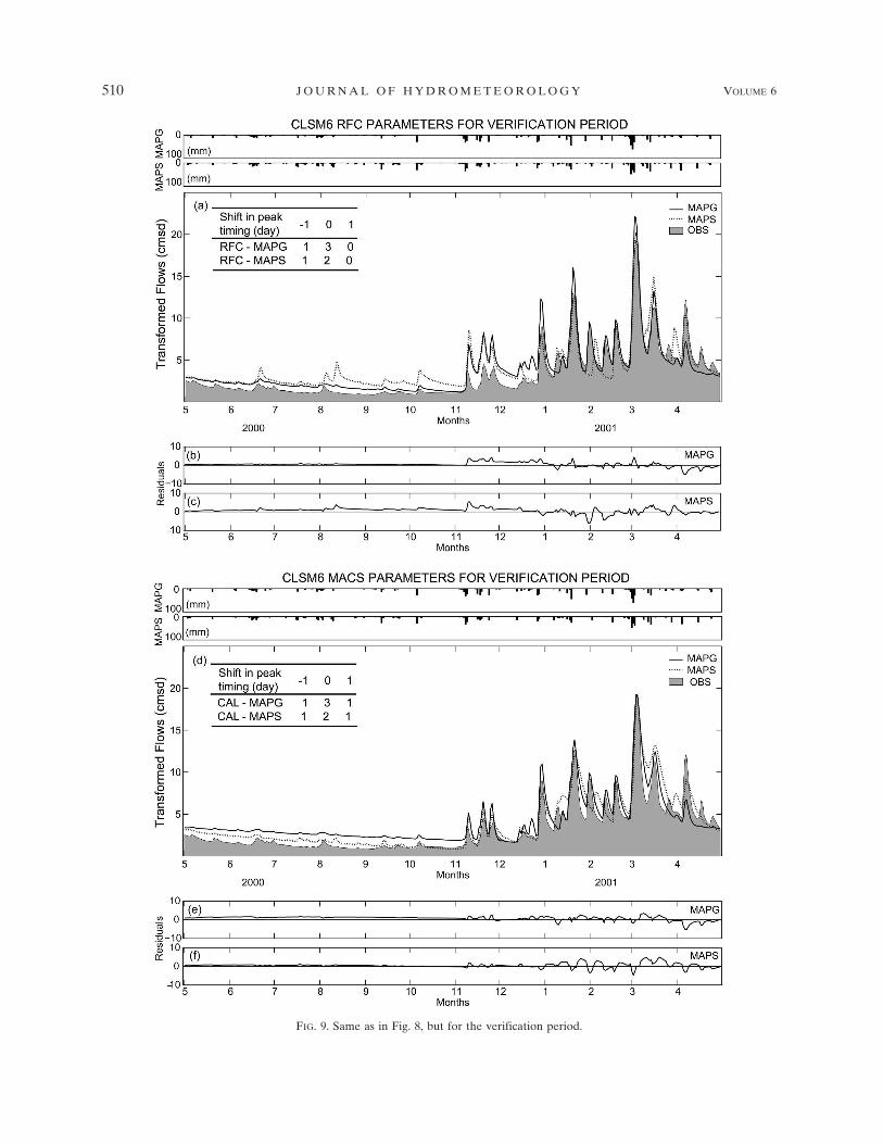
FIG. 9. Same as in Fig. 8, but for the verification period.


FIG. 10. Same as in Fig. 8, but for CLUG1.


FIG. 11. Same as in Fig. 8, but for the CLUG1 verification period.


flow performance over the full range of flows, hydro-graphs are plotted in the transformed space

Qtransformed ��Q � 1�� 1

�, �5�

where Q is the flow and � is a transformation param-eter, which is set to 0.3 (after evaluating the visual ef-fect provided by a full range of � values).

1) RFC PARAMETERS

The overall statistics (Fig. 7) show that the RFC-MAPG simulation generally resulted in reasonableNSE statistics with a minimum for the PLAM6 basin(NSE � 0.5). An exception is the CLSM6 basin wherepoor performance (NSE � 0.1) is observed, possiblydue to the large overestimation of the observed peaksduring October–December 2002 and poor matching ofthe peak timing (Fig. 8a). Overall, a large positive %BIAS results from the RFC-MAPG simulations (reach-ing up to 38% for the PLAM6 basin during the calibra-tion period). Verification period statistics also show alarge positive % BIAS for RFC-MAPG (especially inthe Georgia basins), most likely due to the prevailingdry conditions. RFC-MAPS, on the other hand, re-sulted in negative NSE statistics for CLSM6, DARL1,PLAM6, and CLUG1 basins during the calibration pe-riod, indicating simulation predictions are not as goodas simply using the observed mean as a predictor. In theCLSM6 basin, the RFC-MAPS (Figs. 8a,c) significantlyoverestimated peak flows during spring–summer 2003.A major overestimation is evident around 9 April 2003with an observed peak flow of 266 cm. During thisevent, MAPS reported 197 mm of rainfall in three dayswith a peak flow of 1073 cm (300% BIAS) on the sameday, while MAPG reported 83.5 mm and a peak flow of307 cm (15% BIAS) one day earlier than observed.Overestimation of peak flows during spring and sum-mer are also evident in the PLAM6 and DARL1 basinRFC-MAPS simulations (not shown). In the CLSM6basin, RFC-MAPS (Figs. 8a,c) resulted in a general un-derestimation of flows during the winter, with the ex-ception of several overestimated peak flows (see mid-D e c e m -ber 2002). Throughout the calibration period RFC-MAPS shows both false (mid-May 2003) and missed(mid-October 2002) peak flows, which are properly de-picted by the MAPG.

In the CLUG1 basin, RFC-MAPG results in goodoverall performance (Fig. 7f) (0.87 NSE; 11% BIAS)and a good match between the observed and simulatedhydrographs (Figs. 10a,b). RFC-MAPS, on the otherhand, has particular difficulty with both over- and un-derestimations during winter 2002 and spring 2003. A

major overestimation of peak flow by RFC-MAPS isevident on 9 May 2003 with an observed flow of 1014cm. During this event, MAPS reported 183.7 mm ofrainfall in 4 days with a peak flow of 2235 cm (120%BIAS) while MAPG reported 97 mm and a peak flowof 798 cm (21% BIAS). Another interesting event oc-curs in early October 2002, when RFC-MAPS missed apeak flow, which is properly diagnosed by RFC-MAPG.

During the verification period (Figs. 7g–l), the RFC-MAPS for the CLSM6 and PLAM6 basins show bettermodel performance than the RFC-MAPG as indicatedby higher (lower) NSE (% BIAS). This situation can beexplained using Fig. 9a, in which RFC-MAPG simula-tions overestimated the high-flow events. This resultmay be due to error in the MAPG estimates, but also toerror in the evapotranspiration estimates since overes-timation was also seen in winter/early fall 2002 (Fig.8a).

2) CALIBRATED PARAMETERS

The previous subsection illustrated that model per-formance significantly reduces when utilizing satellite-based precipitation estimates with RFC parameters.This subsection introduces model calibration efforts toanalyze whether an improvement in the performance ofa model driven by MAPS and MAPG can be achievedbased on calibration using a relatively short period ofdata (23 months).

The overall statistics (Figs. 7a–f) show comparativelybetter model performance with calibrated parameterscompared to the RFC parameters for both MAPG andMAPS simulations. In the CLSM6 basin, a significantimprovement in the calibration period is observed forCAL-MAPG when compared to RFC-MAPG (NSEchanged from 0.1 to 0.8), followed however by onlyminor improvement for the verification period. Analy-sis of the hydrographs for the calibration period (Figs.8a–e) shows that the improvement in model perfor-mance is mainly due to the better estimation of flowsduring October–December 2002 and better matchingin timing of the peak flows. Another significant im-provement with CAL-MAPG, both in terms of NSEand % BIAS, is obtained for the PLAM6 basin, whichis also followed by significant improvement in the veri-fication period. For the DARL1, CLUG1, AYSG1,and REDG1 basins, CAL-MAPG resulted in minorimprovements in model performance. CAL-MAPS, onthe other hand, yields performance improvements forevery basin during the calibration period, but theCLSM6 and PLAM6 basins still suffer from poor per-formance. Improvement in model performance forthe CLSM6 basin, when using CAL-MAPS, is mainly


due to a decrease in overestimation of peak flows andalso a better simulation of peak timing (Figs. 8a,d).While parameter adjustments compensated for someof the error in the MAPS input, calibration also re-sulted in increased errors during the recessions and lowflows (see April, May, and August 2003). In theCLUG1 basin (Figs. 7f, 10), model performance im-provement is mainly due to the elimination of false highflows by CAL-MAPS compared to RFC-MAPS. Forexample, the highest observed flow event (1014 cm)occurring on 9 May 2003 was reduced from 2350 cm(120% BIAS) for RFC-MAPS to 1200 cm (18% BIAS)for CAL-MAPS. In the CLUG1 basin, the verificationperformance for CAL-MAPS (0.65 NSE and �6.5%BIAS) is in line with the calibration performance andslightly poorer than the CAL-MAPG performance dur-ing verification (0.89 NSE and �7.5% BIAS). In theCLUG1 basin verification period (Fig. 11d), both CAL-MAPS and CAL-MAPG had difficulty in predictingpeak flows during March–April 2001, but CAL-MAPGbetter represented the lower peak flows (see Septem-ber and December 2000).

In the AYSG1 basin (Figs. 7e,k), although the cali-brated parameters resulted in slightly improved per-formance over the RFC parameters during the calibra-tion period, they failed to capture the observed flowsduring the verification period (NSE ��1 and BIAS�100%). The REDG1 basin (Figs. 7d,j) shows im-proved model performance due to model calibration,not only during the calibration period but also duringthe verification period. In the verification period, CAL-MAPS resulted in even better performance than CAL-MAPG. Analysis of the hydrographs (not shown) indi-cates that both CAL-MAPG and CAL-MAPS tend tostrongly overestimate the dry conditions prevailing dur-ing May–September 2000 in the REDG1 basin, but italso revealed that the CAL-MAPG simulations over-estimate the relatively high flow conditions during win-ter/spring 2001. The SERFC has also reported particu-lar difficulty in calibration of the AYSG1 and REDG1basins (J. Bradberry, SERFC, 2004, personal commu-nication).

As an overall summary, calibration of the SAC-SMAmodel with satellite precipitation estimates has im-proved the model performance in both the calibrationand verification periods when compared to the modelsimulations with RFC parameters. But MAPS-drivenmodel performances were still poor for the PLAM6,DARL1, and CLSM6 basins, which are smaller in sizeand produced high biases between MAPG and MAPS.Poor model performance even for the calibration pe-riod is an indication of an inability of the model and the

calibration procedure to filter out the variation and er-ror in MAPS. Better performances obtained for theCLUG1 (slightly poorer than rain gauge calibration)and REDG1 (better than rain gauge calibration duringverification period) basins are probably due to the largesize of these basins and a smaller bias between MAPGand MAPS. Again, note that short calibration and veri-fication time periods may also have an effect on theseresults.

6. Conclusions and recommendations

The objective of this study was to evaluate the utilityof satellite-based precipitation estimates for hydrologicforecasting, as they may provide the only source of pre-cipitation for areas where ground-based networks areunavailable. The results of our precipitation intercom-parison study performed at seven basins within thesoutheastern United States show that agreements be-tween the precipitation datasets vary from basin to ba-sin and also temporally within the basins. General con-clusions from the three-way intercomparison of thedatasets are provided below. Please note that these arerelative comparisons only.

1) MAPS tends to provide larger estimates thanMAPG during the warm season and smaller esti-mates than MAPG during the cold season for thebasins located in Mississippi, Louisiana, and Arkan-sas. This warm-season trend is most pronounced forthe Arkansas basin. In the Georgia basins, a sea-sonal trend was not evident between the MAPG andMAPS, and fairly good agreements in terms ofmonthly totals and overall bias were observed.

2) MAPX tends to provide slightly larger estimatesthan MAPG for the basins in Louisiana and Arkan-sas regardless of the season; however, this tendencyis more pronounced during the warm season. In theMississippi basins, MAPX tends to provide largerestimates than MAPG during the warm season andsmaller estimates during the cold season. In theGeorgia basins, the MAPX–MAPG comparisonshows large variation. MAPX provides considerablylarger estimates than MAPG during the warm sea-son in the earlier time periods, but better agreement(with slightly smaller estimates) in the later timeperiod. This change is probably due to the change inthe radar-processing algorithm (from stage III toMPE) implemented by the SERFC. At the 6-h timescale, the correlation between MAPX and MAPG ishigher for winter stratiform precipitation than sum-mer convective precipitation. This difference is


more pronounced for the two basins in Georgia, inwhich a fewer hourly rain gauges are present.

3) The MAPS–MAPX comparison shows smaller biasthan the MAPS–MAPG comparison at some timeperiods but larger bias in other periods. This ismainly due to a similar MAPX and MAPS responseto stratiform and convective precipitation patternsin some basins (although for different reasons), butis complicated by calibration differences betweenradars, availability of hourly rain gauges for radarbias correction, degree of radar quality control, andgeographic location.

Results from the evaluation of the hydrologicalmodel performance show that, when using satellite-based precipitation estimates, even short time periodsof model calibration can considerably improve modelperformance compared to manually calibrated param-eters using historical rain gauge data (RFC param-eters). Of course, the degree of improvement may varywith basin size and location. These results can be sum-marized as follows.

1) When MAPS is used to drive the model with RFCparameters, major deterioration in model perfor-mance is observed when compared with the MAPG-driven model. We observe positive streamflow pre-diction bias in all study basins, and negative Nash–Sutcliffe efficiencies in four out of six basins.Calibration improves model performance in all ba-sins as expected, but the results are not satisfactoryfor basins in Mississippi and Louisiana (even for thecalibration period). The better calibration perfor-mance obtained with MAPG (indicated by NSE and% BIAS statistics) suggests problems with theMAPS product. The poor MAPS results may be at-tributed to the large differences between MAPS andMAPG over these basins, which may be partly dueto the fact that these basins are smaller in size andtherefore there is less smoothing of the precipitationvariation and error. For the two Georgia basins,model calibration using MAPS resulted in signifi-cantly improved model performance (for both cali-bration and verification periods)—these are also thebasins showing better agreement between MAPSand MAPG. Note, however, that for all the studiesconducted here the calibration and verification pe-riods used were for relatively short and dry condi-tions—those results should therefore be only viewedas preliminary.

2) Changes/improvements in the radar/gauge multisen-sor precipitation-processing algorithms (such astransition from stage III to MPE) affect the behav-ioral characteristics of this dataset. These behavior-

al changes must be properly taken into accountwhen such data are used for model calibration and/or evaluation in future studies.

As a future extension of this analysis, different hy-droclimatic regions (e.g., semiarid) over different partsof the world will be selected with varying basin sizesand rain gauge network densities to further test thepossible benefits of using satellite-based precipitationestimates for flow prediction. The availability of theseestimates at finer spatial scales will improve their ap-plicability to basin-scale hydrologic applications, espe-cially when using distributed models. Also, inclusion oferror estimates associated with satellite-based precipi-tation products will enable hydrologists to define con-fidence limits on the hydrologic predictions. As a natu-ral extension of this work for ungauged basin studies,satellite-based precipitation estimates will be used to-gether with model parameters derived from basin char-acteristics, rather than calibrated through observedstreamflow.

We have demonstrated that although satellite-basedprecipitation estimates contain errors that can affectflow predictions, there is clear potential for use ofthese products in hydrologic forecasting and watermanagement. This potential is expected to increasewith the launch of new satellites. The neural networkstructure of the PERSIANN system can easily beadapted to incorporate new information as it becomesavailable.

Acknowledgments. Support for this work was pro-vided by NASA Jet Propulsion Laboratory (Grant1236728), the Center for Sustainability of semi-AridHydrology and Riparian Areas (SAHRA) (EAR-9876800), the Hydrology Laboratory of the NationalWeather Service (Grants NA87WHO582 andNA07WH0144), NASA-EOS (Grant NA56GPO185),TRMM (Grant NAG5-7716), and the InternationalCentre for Scientific Culture—World Laboratory. Wethank the personnel of Lower Mississippi and South-east River Forecast Centers for their help and guid-ance. We would also like to thank David R. Legatesand anonymous reviewers for their constructive com-ments.

REFERENCES

Adler, R. F., G. J. Huffman, D. T. Bolvin, S. Curtis, and E. J.Nelkin, 2000: Tropical rainfall distributions determined usingTRMM combined with other satellite and rain gauge infor-mation. J. Appl. Meteor., 39, 2007–2023.

——, C. Kidd, G. Petty, M. Morrissey, and H. M. Goodman, 2001:Intercomparison of global precipitation products: The third


Precipitation Intercomparison Project (PIP-3). Bull. Amer.Meteor. Soc., 82, 1377–1396.

Andreassian, V., C. Perrin, C. Michel, I. Usart-Sanchez, and J.Lavabre, 2001: Impact of imperfect rainfall knowledge on theefficiency and the parameters of watershed models. J. Hy-drol., 250, 206–223.

Brazil, L. E., and M. D. Hudlow, 1981: Calibration proceduresused with the National Weather Service River Forecast Sys-tem. Water and Related Land Resource Systems, Y. Y.Haimes and J. Kindler, Eds., Pergamon, 457–566.

Burnash, R. J. C., 1995: The NWS River Forecast System—Catchment modeling. Computer Models of Watershed Hy-drology, V. P. Singh, Ed., Water Resources Publications,311–366.

——, R. L. Ferral, and R. A. McGuire, 1973: A generalizedstreamflow simulation system—Conceptual modeling fordigital computers. Joint Federal–State River Forecast CenterTech. Rep., Department of Water Resources, State of Cali-fornia and National Weather Service, 204 pp.

Duan, Q. Y., S. Sorooshian, and H. V. Gupta, 1992: Effective andefficient global optimization for conceptual rainfall-runoffmodels. Water Resour. Res., 28, 1015–1031.

Ferraro, R. R., and G. F. Marks, 1995: The development of SSM/Irain-rate retrieval algorithms using ground-based radar mea-surements. J. Atmos. Oceanic Technol., 12, 755–770.

Finnerty, B. D., M. B. Smith, D.-J. Seo, V. Koren, and G. E. Mo-glen, 1997: Space–time scale sensitivity of the Sacramentomodel to radar-gage precipitation inputs. J. Hydrol., 203, 21–38.

Fulton, R. A., 2002: Activities to improve WSR-88D radar rainfallestimation in the National Weather Service. Proc. SecondFederal Interagency Hydrologic Modeling Conf., Las Vegas,NV, Subcomittee on Hydrology, Advisory Committee onWater Data, CD-ROM. [Available online at http://www.nws.noaa.gov/oh/hrl/presentations/fihm02/pdfs/qpe_hydromodelconf_web.pdf.]

——, J. P. Breidenbach, D.-J. Seo, D. A. Miller, and T. O’Bannon,1998: The WSR-88D rainfall algorithm. Wea. Forecasting, 13,377–395.

Grassotti, C., R. N. Hoffman, E. R. Vivoni, and D. Entekhabi,2003: Multiple-timescale intercomparison of two radar prod-ucts and rain gauge observations over the Arkansas–RedRiver basin. Wea. Forecasting, 18, 1207–1229.

Grimes, D. I. F., and M. Diop, 2003: Satellite-based rainfall esti-mation for river flow forecasting in Africa. I: Rainfall esti-mates and hydrological forecasts. Hydrol. Sci. J., 48, 567–584.

Groisman, P. Y., and D. R. Legates, 1994: The accuracy of UnitedStates precipitation data. Bull. Amer. Meteor. Soc., 75, 215–227.

Gupta, H. V., K. J. Beven, and T. Wagener, 2005: Model calibra-tion and uncertainty estimation. Encyclopedia of Hydrologi-cal Sciences, M. G. Anderson, Ed., John Wiley & Sons, inpress.

Hogue, T. S., S. Sorooshian, H. V. Gupta, A. Holz, and D. Braatz,2000: A multistep automatic calibration scheme for riverforecasting models. J. Hydrometeor., 1, 524–542.

Hsu, K., X. Gao, S. Sorooshian, and H. V. Gupta, 1997: Precipi-tation estimation from remotely sensed information using ar-tificial neural networks. J. Appl. Meteor., 36, 1176–1190.

——, H. V. Gupta, X. Gao, and S. Sorooshian, 1999: Estimation ofphysical variables from multiple channel remotely sensed im-agery using a neural network: Application to rainfall estima-tion. Water Resour. Res., 35, 1605–1618.

——, ——, ——, ——, and B. Imam, 2002: Self-organizing linearoutput map (SOLO): An artificial neural network suitablefor hydrologic modeling and analysis. Water Resour. Res., 38,1302, doi:10.1029/2001WR000795.

Huffman, G. J., R. F. Adler, M. Morrissey, D. T. Bolvin, S. Curtis,R. Joyce, B. McGavock, and J. Susskind, 2001: Global pre-cipitation at one-degree daily resolution from multisatelliteobservations. J. Hydrometeor., 2, 36–50.

Johnson, D., M. Smith, V. Koren, and B. Finnerty, 1999: Com-paring mean areal precipitation estimates from NEXRADand rain gauge networks. J. Hydrol. Eng., 2, 117–124.

Kidd, C., 2001: Satellite rainfall climatology: A review. Int. J. Cli-matol., 21, 1041–1066.

Koren, V. I., B. D. Finnerty, J. C. Schaake, M. B. Smith, D.-J. Seo,and Q. Y. Duan, 1999: Scale dependencies of hydrologicmodels to spatial variability of precipitation. J. Hydrol., 217,285–302.

Krajewski, W. F., G. J. Ciach, J. R. McCollum, and C. Bacotiu,2000: Initial validation of the Global Precipitation Climatol-ogy Project monthly rainfall over the United States. J. Appl.Meteor., 39, 1071–1086.

Kuligowski, R. J., 2002: A self-calibrating real-time GOES rainfallalgorithm for short-term rainfall estimates. J. Hydrometeor.,3, 112–130.

Kummerow, C., W. Barnes, T. Kozu, J. Shiue, and J. Simpson,1998: The Tropical Rainfall Measuring Mission (TRMM)sensor package. J. Atmos. Oceanic Technol., 15, 809–816.

Legates, D. R., and T. L. DeLiberty, 1993: Precipitation measure-ment biases in the United States. Water Resour. Bull., 29,855–861.

McCollum, J. R., W. F. Krajewski, R. R. Ferraro, and M. B. Ba,2002: Evaluation of biases of satellite rainfall estimation al-gorithms over the continental United States. J. Appl. Meteor.,41, 1065–1080.

Morin, E., W. F. Krajewski, D. C. Goodrich, X. Gao, and S. So-rooshian, 2003: Estimating rainfall intensities from weatherradar data: The scale-dependency problem. J. Hydrometeor.,4, 782–797.

Petty, G., and W. F. Krajewski, 1996: Satellite estimation of pre-cipitation over land. Hydrol. Sci. J., 41, 433–451.

Rozumalski, R. A., 2000: A quantitative assessment of theNESDIS Auto-Estimator. Wea. Forecasting, 15, 397–415.

Scofield, R. A., and R. J. Kuligowski, 2003: Status and outlook ofoperational satellite precipitation algorithms for extreme-precipitation events. Wea. Forecasting, 18, 1037–1051.

Seo, D.-J., R. A. Fulton, and J. P. Breidenbach, 1997: Interagencymemorandum of understanding among the NEXRAD pro-gram, WSR-88D Operational Support Facility, and the NWS/OH Hydrologic Research Laboratory. NWS/OH HydrologicResearch Laboratory Final Report, Silver Spring, MD.[Available from NWS/OH/HRL, 1325 East–West Hwy.,W/OH1, Silver Spring, MD 20910.]

Sivapalan, M., and Coauthors, 2003: IAHS decade on Predictionsin Ungauged Basins (PUB), 2003–2012: Shaping an excitingfuture for the hydrological sciences. Hydrol. Sci. J., 48, 857–880.

Smith, J. A., D. J. Seo, M. L. Baeck, and M. D. Hudlow, 1996: Anintercomparison study of NEXRAD precipitation estimates.Water Resour. Res., 32, 2035–2045.

Sorooshian, S., K. Hsu, X. Gao, H. V. Gupta, B. Imam, and D.Braithwaite, 2000: Evaluation of PERSIANN system satel-


lite-based estimates of tropical rainfall. Bull. Amer. Meteor.Soc., 81, 2035–2046.

Stellman, K. M., H. E. Fuelberg, R. Garza, and M. Mullusky,2001: An examination of radar and rain gauge–derived meanareal precipitation over Georgia watersheds. Wea. Forecast-ing, 16, 133–144.

Tsintikidis, D., K. P. Georgakakos, G. A. Artan, and A. A. Tso-nis, 1999: A feasibility study on mean areal rainfall estimationand hydrologic response in the Blue Nile region usingMETEOSAT images. J. Hydrol., 221, 97–116.

Weng, F., L. Zhao, R. R. Ferraro, G. Poe, X. Li, and N. C. Grody,2003: Advanced microwave sounding unit cloud and precipi-tation algorithms. Radio Sci., 38, 8068, doi:10.1029/2002RS002679.

Winchell, M., H. V. Gupta, and S. Sorooshian, 1998: On the simu-

lation of infiltration- and saturation-excess runoff using ra-dar-based rainfall estimates: Effects of algorithm uncertaintyand pixel aggregation. Water Resour. Res., 34, 2655–2670.

Xie, P., and P. A. Arkin, 1995: An intercomparison of gauge ob-servations and satellite estimates of monthly precipitation. J.Appl. Meteor., 34, 1143–1160.

——, and ——, 1997: Global precipitation: A 17-year monthlyanalysis based on gauge observations, satellite estimates, andnumerical model outputs. Bull. Amer. Meteor. Soc., 78, 2539–2558.

Young, C. B., A. A. Bradley, W. F. Krajewski, A. Kruger, andM. L. Morrissey, 2000: Evaluating NEXRAD multisensorprecipitation estimates for operational hydrologic forecast-ing. J. Hydrometeor., 1, 241–254.


intercomparison of rain gauge, radar, and satellite-based...

Documents