interface(rtablesize=20): linear elliptic pdes: solution of ... concreteness, we will focus on the...
TRANSCRIPT
> >
> >
restart:with(LinearAlgebra):with(plots):with(PDEtools):interface(rtablesize=20):
Linear elliptic PDEs: solution of Laplace and Poisson equations in 2DThe purpose of this worksheet is to illsutrate how to solve linear elliptic PDEs. For concreteness, we will focus on the following PDE:
v2uvx2 C
v2uvy2 = f x, y ,
where the source function f x, y is given. If f x, y = 0 this is known as Laplace's equation, if not it is Poisson's equation. We will seek a solution on a rectangular region of the xy-plane: x, y 2 KL, L # KL, L subject to Dirichlet boundary conditions:
u x, y =KL = g1 x , u x =CL, y = g2 y , u x, y =CL = g3 x , u x =KL, y = g4 y , .
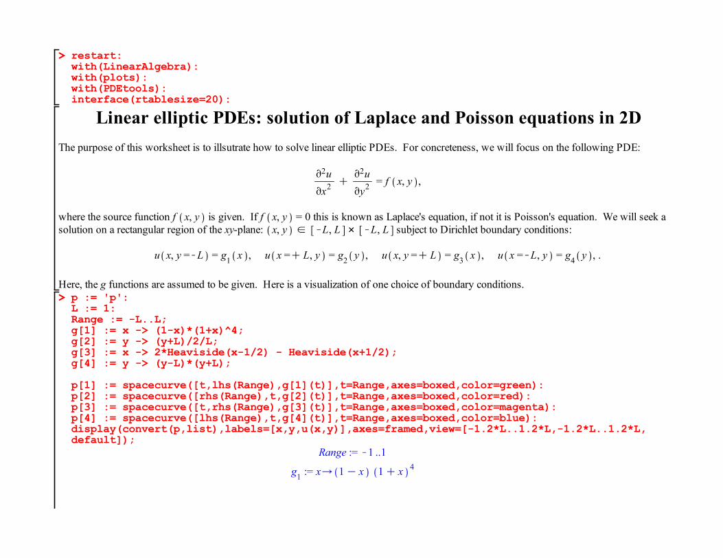
Here, the g functions are assumed to be given. Here is a visualization of one choice of boundary conditions.p := 'p':L := 1:Range := -L..L;g[1] := x -> (1-x)*(1+x)^4;g[2] := y -> (y+L)/2/L;g[3] := x -> 2*Heaviside(x-1/2) - Heaviside(x+1/2);g[4] := y -> (y-L)*(y+L);
p[1] := spacecurve([t,lhs(Range),g[1](t)],t=Range,axes=boxed,color=green):p[2] := spacecurve([rhs(Range),t,g[2](t)],t=Range,axes=boxed,color=red):p[3] := spacecurve([t,rhs(Range),g[3](t)],t=Range,axes=boxed,color=magenta):p[4] := spacecurve([lhs(Range),t,g[4](t)],t=Range,axes=boxed,color=blue):display(convert(p,list),labels=[x,y,u(x,y)],axes=framed,view=[-1.2*L..1.2*L,-1.2*L..1.2*L,default]);
Range := K1 ..1
g1 := x/ 1K x 1C x 4

g2 := y/12
yCL
L
g3 := x/2 Heaviside xK12
KHeaviside xC12
g4 := y/ yKL yCL

> >
> >
(1.1)(1.1)
In this plot, the desired values of u x, y are shown on the boundary of the region we are interested in. The goal of the numerical analysis will to be to "fill-in" the values of u x, y interior to the boundary.
Numerical solution using a five-point stencil for the LaplacianIn this section, we will develop the solution to the following PDE assuming a stencil for the differential operator involving five points:pde := diff(u(x,y),x,x) + diff(u(x,y),y,y) - f(x,y);
pde := v2
vx2 u x, y Cv2
vy2 u x, y K f x, y
StencilAs usual, we make use of the GenerateStencil procedure:GenerateStencil := proc(F,N,{orientation:=center,stepsize:=h,showorder:=true,showerror:=false}) local vars, f, ii, Degree, stencil, Error, unknowns, Indets, ans, Phi, r, n, phi;
Phi := convert(F,D); vars := op(Phi); n := PDEtools[difforder](Phi); f := op(1,op(0,Phi)); if (nops([vars])<>1) then: r := op(1,op(0,op(0,Phi))); else: r := 1; fi: phi := f(vars); if (orientation=center) then: if (type(N,odd)) then: ii := [seq(i,i=-(N-1)/2..(N-1)/2)]; else: ii := [seq(i,i=-(N-1)..(N-1),2)]; fi; elif (orientation=left) then: ii := [seq(i,i=-N+1..0)]: elif (orientation=right) then: ii := [seq(i,i=0..N-1)]: fi; stencil := add(a[ii[i]]*subsop(r=op(r,phi)+ii[i]*stepsize,phi),i=1..N);

> >
> >
> >
(1.1.2)(1.1.2)
(1.1.1)(1.1.1)
Error := D[r$n](f)(vars) - stencil; Error := convert(series(Error,stepsize,N),polynom); unknowns := {seq(a[ii[i]],i=1..N)}; Indets := indets(Error) minus {vars} minus unknowns minus {stepsize}; Error := collect(Error,Indets,'distributed'); ans := solve({coeffs(Error,Indets)},unknowns); if (ans=NULL) then: print(`Failure: try increasing the number of points in the stencil`); return NULL; fi: stencil := subs(ans,stencil); Error := convert(series(`leadterm`(D[r$n](f)(vars) - stencil),stepsize,N+20),polynom); Degree := degree(Error,stepsize); if (showorder) then: print(cat(`This stencil is of order `,Degree)); fi: if (showerror) then: print(cat(`This leading order term in the error is `,Error)); fi: convert(D[r$n](f)(vars) = stencil,diff);
end proc:We will use centered stencils for the second derivatives in the x and y directions:substencil[1] := GenerateStencil(diff(u(x,y),x,x),3);substencil[2] := GenerateStencil(diff(u(x,y),y,y),3);
This stencil is of order 2
substencil1 := v2
vx2 u x, y =u xK h, y
h2 K2 u x, y
h2 Cu xC h, y
h2
This stencil is of order 2
substencil2 := v2
vy2 u x, y =u x, yK h
h2 K2 u x, y
h2 Cu x, yC h
h2
Notice that we have assumed the same stepsize h in the x and y directions. Putting these into (1.1) gives:stencil[1] := subs(substencil[1],substencil[2],pde);
stencil1 :=u xK h, y
h2 K4 u x, y
h2 Cu xC h, y
h2 Cu x, yK h
h2 Cu x, yC h
h2 K f x, y
> >
> >
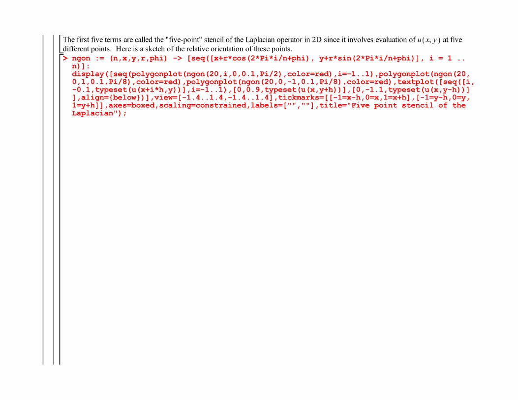
The first five terms are called the "five-point" stencil of the Laplacian operator in 2D since it involves evaluation of u x, y at five different points. Here is a sketch of the relative orientation of these points.ngon := (n,x,y,r,phi) -> [seq([x+r*cos(2*Pi*i/n+phi), y+r*sin(2*Pi*i/n+phi)], i = 1 .. n)]:display([seq(polygonplot(ngon(20,i,0,0.1,Pi/2),color=red),i=-1..1),polygonplot(ngon(20,0,1,0.1,Pi/8),color=red),polygonplot(ngon(20,0,-1,0.1,Pi/8),color=red),textplot([seq([i,-0.1,typeset(u(x+i*h,y))],i=-1..1),[0,0.9,typeset(u(x,y+h))],[0,-1.1,typeset(u(x,y-h))]],align={below})],view=[-1.4..1.4,-1.4..1.4],tickmarks=[[-1=x-h,0=x,1=x+h],[-1=y-h,0=y,1=y+h]],axes=boxed,scaling=constrained,labels=["",""],title="Five point stencil of the Laplacian");

> >
(1.1.3)(1.1.3)
> >
u xK h, y u x, y u xC h, y
u x, yC h
u x, yK h
x K h x x C h
y K h
y
y C h
Five point stencil of the Laplacian
Let's check the error in the stencil by expanding in a Taylor series and then making use of the original PDE:Error := series(stencil[1],h,8):Error := convert(dsubs(isolate(pde,f(x,y)),Error),D);
Error :=112
D1, 1, 1, 1 u x, y C112
D2, 2, 2, 2 u x, y h2 C1
360 D2, 2, 2, 2, 2, 2 u x, y

(1.1.4)(1.1.4)
> >
(1.1.6)(1.1.6)
> >
(1.2.1)(1.2.1)
> >
(1.1.5)(1.1.5)
> >
(1.1.3)(1.1.3)
> >
C1
360 D1, 1, 1, 1, 1, 1 u x, y h4 CO h6
It is common in the literature to conclude from this result that the error in the stencil is O h2 . However, some care is warranted with this terminology since it relies on the stencil being written precisely in the form of (1.1.2); i.e., on the u terms all being divided by h2. If we had instead written our stencil as:alt_stencil := expand(h^2*stencil[1]);
alt_stencil := u xK h, y K 4 u x, y C u xC h, y C u x, yK h C u x, yC h K h2 f x, y
and expanded about h = 0 the leading order behaviour would have been O h4 : alt_Error := series(alt_stencil,h,6):alt_Error := convert(dsubs(isolate(pde,f(x,y)),alt_Error),D);
alt_Error :=112
D1, 1, 1, 1 u x, y C112
D2, 2, 2, 2 u x, y h4 CO h6
The common definition of error for the numeric solution PDEs involves first writing the stencil in a form whose limit is the original PDEas the cell size goes to zero:limit(stencil[1],h=0);limit(alt_stencil,h=0);
D2, 2 u x, y CD1, 1 u x, y K f x, y
0
We see that stencil matches this requirement, but alt_stencil does not. The error is then defined as the discrepancy between the stencil written in the perferred form and zero; i.e., what we have called Error but not what we've called alt_Error.
The algorithmHaving now obtained a discrete form (1.1.2) of the PDE (1.1), we now turn our attention to how to exploit it and obtain a numeric solution. We first need to discretize the domain x, y 2 a, b # c, d over which we seek a solution. We will assume NC 2 lattice points in the x and y directions, respectively. The coordinates of the lattice point will be explicitly given by xi = Z i and yj = Z j , whereL := 'L':N := 'N':g := 'g':Z := i -> -L+2*L/(N+1)*i;x[0] = Z(0),x[N+1] = Z(N+1),y[0] = Z(0),y[N+1] = Z(N+1);

> >
> >
(1.2.1)(1.2.1)
(1.1.3)(1.1.3)
Z := i/KL C2 L i
NC 1x0 = KL, xN C 1 = L, y0 = KL, yN C 1 = L
Here is a visualization of the lattice:N := 4;L := 1;r := L/(N+1)/4;ngon := (n,x,y,r,phi) -> [seq([x+r*cos(2*Pi*i/n+phi), y+r*sin(2*Pi*i/n+phi)], i = 1 .. n)]:p[1] := display([seq(polygonplot(ngon(4,Z(0),Z(j),r,Pi/2),color=magenta),j=0..N+1),seq(polygonplot(ngon(4,Z(N+1),Z(j),r,Pi/2),color=magenta),j=0..N+1),seq(polygonplot(ngon(4,Z(i),Z(0),r,0),color=magenta),i=1..N),seq(polygonplot(ngon(4,Z(i),Z(N+1),r,0),color=magenta),i=1..N),seq(seq(polygonplot(ngon(20,Z(i),Z(j),r,0),color=white),i=1..N),j=1..N),textplot([seq(seq([Z(i+0.1),Z(j),typeset(u[i,j])],i=0..N+1),j=0..N+1)],align={above,right})],view=[Z(-1)..Z(N+2),Z(-1)..Z(N+2)],tickmarks=[[seq(Z(i)=typeset(x[i]=evalf[2](Z(i))),i=0..N+1)],[seq(Z(i)=typeset(y[i]=evalf[2](Z(i))),i=0..N+1)]],axes=boxed,scaling=constrained,labels=[``,``]):p[1];
N := 4L := 1
r :=120

(1.2.1)(1.2.1)
(1.1.3)(1.1.3)
> >
u0, 0 u1, 0 u2, 0 u3, 0 u4, 0 u5, 0
u0, 1 u1, 1 u2, 1 u3, 1 u4, 1 u5, 1
u0, 2 u1, 2 u2, 2 u3, 2 u4, 2 u5, 2
u0, 3 u1, 3 u2, 3 u3, 3 u4, 3 u5, 3
u0, 4 u1, 4 u2, 4 u3, 4 u4, 4 u5, 4
u0, 5 u1, 5 u2, 5 u3, 5 u4, 5 u5, 5
x0 = K1. x1 = K0.6 x2 = K0.2 x3 = 0.2 x4 = 0.6 x5 = 1.
y0 = K1.
y1 = K0.6
y2 = K0.2
y3 = 0.2
y4 = 0.6
y5 = 1.

> >
(1.2.2)(1.2.2)
> >
(1.2.4)(1.2.4)
> >
(1.2.1)(1.2.1)
> >
(1.2.3)(1.2.3)
(1.1.3)(1.1.3)
Each node is labelled by our approximation to the true solution of the PDE ui, j z u xi, yj . Boundary conditions will be used to fix ui, j at each of the purple boundary nodes, so the goal of the code will be to solve for ui, j at each of the white interior nodes. We also define fi, j = f xi, yj , which allows us to re-write the stencil (1.1.2) as:Subs := seq(seq(u(x+ii*h,y+jj*h)=u[i+ii,j+jj],ii=-1..1),jj=-1..1),f(x,y)=f[i,j]:stencil[1] := subs(Subs,stencil[1]);
stencil1 :=ui K 1, j
h2 K4 ui, j
h2 Cui C 1, j
h2 Cui, j K 1
h2 Cui, j C 1
h2 K fi, j
We will enforce this stencil for i = 1 ... N and j = 1 ... N; i.e., at each of the white circles in the above plot. To do this, it is useful to rewrite the stencil as a mapping:Stencil[1] := unapply(stencil[1],h,i,j,u,f);
Stencil1 := h, i, j, u, f /
ui K 1, j
h2 K4 ui, j
h2 Cui C 1, j
h2 Cui, j K 1
h2 Cui, j C 1
h2 K fi, j
Here is an example of the kind of system of equations we need to solve for N 2 = 9 total internal lattice points. The boundary conditions u x,KL = g1 x , etc. are implemented by assigning values to all the boundary nodes (purple diamonds in the above sketch). For example, we set u0, i = g1 xi . The boundary conditions are held in the list BCs.
Aside: There is a potential conflict at the corners of our lattice where i, j = 0, 0 , NC 1, 0 , NC 1 , NC 1 , 0, NC 1 if g1 L s g2 KL , g2 KL s g3 L , g3 KL s g4 L , or g4 KL s g1 KL . Ideally, we should choose boundary data to ensure that this does not happen, but if there is an ambiguity we will (arbitrarily) assume that the top and bottom boundary data (g1 and g3) take precedence over the left and right boundary data (g2 and g4).N := 3:
BCs := [seq(u[0,i] =g[4](y[i]),i=1..N), seq(u[i,0] =g[1](x[i]),i=0..N+1), seq(u[N+1,i]=g[2](y[i]),i=1..N), seq(u[i,N+1]=g[3](x[i]),i=0..N+1)]:
sys := Vector([subs(BCs,[seq(seq(Stencil[1](h,i,j,u,f),i=1..N),j=1..N)])]);

(1.2.4)(1.2.4)
> >
(1.2.1)(1.2.1)
> >
(1.1.3)(1.1.3)
sys :=
g4 y1
h2 K4 u1, 1
h2 Cu2, 1
h2 Cg1 x1
h2 Cu1, 2
h2 K f1, 1
u1, 1
h2 K4 u2, 1
h2 Cu3, 1
h2 Cg1 x2
h2 Cu2, 2
h2 K f2, 1
u2, 1
h2 K4 u3, 1
h2 Cg2 y1
h2 Cg1 x3
h2 Cu3, 2
h2 K f3, 1
g4 y2
h2 K4 u1, 2
h2 Cu2, 2
h2 Cu1, 1
h2 Cu1, 3
h2 K f1, 2
u1, 2
h2 K4 u2, 2
h2 Cu3, 2
h2 Cu2, 1
h2 Cu2, 3
h2 K f2, 2
u2, 2
h2 K4 u3, 2
h2 Cg2 y2
h2 Cu3, 1
h2 Cu3, 3
h2 K f3, 2
g4 y3
h2 K4 u1, 3
h2 Cu2, 3
h2 Cu1, 2
h2 Cg3 x1
h2 K f1, 3
u1, 3
h2 K4 u2, 3
h2 Cu3, 3
h2 Cu2, 2
h2 Cg3 x2
h2 K f2, 3
u2, 3
h2 K4 u3, 3
h2 Cg2 y3
h2 Cu3, 2
h2 Cg3 x3
h2 K f3, 3
This is a linear system in the ui, j's. Though it is natural to think of the ui, j's to be arranged in a matrix, it is more convenient to reshape them into a vector as indicated by this before and after plot:p[1] := display([seq(polygonplot(ngon(4,Z(0),Z(j),r,Pi/2),color=magenta),j=0..N+1),seq(polygonplot(ngon(4,Z(N+1),Z(j),r,Pi/2),color=magenta),j=0..N+1),seq(polygonplot(ngon(4,Z(i),Z(0),r,0),color=magenta),i=1..N),seq(polygonplot(ngon(4,Z(i),Z(N+1),r,0),color=magenta),i=1..N),seq(seq(polygonplot(ngon(20,Z(i),Z(j),r,0),color=white),i=1..N),j=1..N),textplot([seq(seq([Z(i+0.1),Z(j),typeset(u[i,j])],i=1..N),j=1..N)],align={above,right})],view=[Z(-1)..Z(N+2),Z(-1)..Z(N+2)],tickmarks=[[seq(Z(i)=typeset(x[i]=evalf[2](Z

(1.2.4)(1.2.4)
> >
(1.2.1)(1.2.1)
> >
(1.1.3)(1.1.3)
(i))),i=0..N+1)],[seq(Z(i)=typeset(y[i]=evalf[2](Z(i))),i=0..N+1)]],axes=boxed,scaling=constrained,labels=[``,``],title="Before re-labelling"):
p[2] := display([seq(polygonplot(ngon(4,Z(0),Z(j),r,Pi/2),color=magenta),j=0..N+1),seq(polygonplot(ngon(4,Z(N+1),Z(j),r,Pi/2),color=magenta),j=0..N+1),seq(polygonplot(ngon(4,Z(i),Z(0),r,0),color=magenta),i=1..N),seq(polygonplot(ngon(4,Z(i),Z(N+1),r,0),color=magenta),i=1..N),seq(seq(polygonplot(ngon(20,Z(i),Z(j),r,0),color=white),i=1..N),j=1..N),textplot([seq(seq([Z(i+0.1),Z(j),typeset(w[(j-1)*N+i])],i=1..N),j=1..N)],align={above,right})],view=[Z(-1)..Z(N+2),Z(-1)..Z(N+2)],tickmarks=[[seq(Z(i)=typeset(x[i]=evalf[2](Z(i))),i=0..N+1)],[seq(Z(i)=typeset(y[i]=evalf[2](Z(i))),i=0..N+1)]],axes=boxed,scaling=constrained,labels=[``,``],title="After re-labelling"):
display(Array(1..2,[p[1],p[2]]));

(1.2.5)(1.2.5)
(1.2.4)(1.2.4)
> >
(1.2.1)(1.2.1)
> >
> >
(1.1.3)(1.1.3)
u1, 1 u2, 1 u3, 1
u1, 2 u2, 2 u3, 2
u1, 3 u2, 3 u3, 3
x0 = K1. x2 = 0. x4 = 1.
y0 = K1.
y1 = K0.5
y2 = 0.
y3 = 0.5
y4 = 1.
Before re-labelling
w1 w2 w3
w4 w5 w6
w7 w8 w9
x0 = K1. x2 = 0. x4 = 1.
y0 = K1.
y1 = K0.5
y2 = 0.
y3 = 0.5
y4 = 1.
After re-labelling
In other words, we re-label the ui, j sequentially by rows. With this understanding (1.2.4) is seen to be a linear system Aw = b withw := [seq(seq(u[i,j],i=1..N),j=1..N)];A,b := GenerateMatrix(convert(sys,list),w);
w := u1, 1, u2, 1, u3, 1, u1, 2, u2, 2, u3, 2, u1, 3, u2, 3, u3, 3

(1.2.5)(1.2.5)
(1.2.4)(1.2.4)
> >
(1.2.1)(1.2.1)
> >
> >
(1.1.3)(1.1.3)
A, b :=
K4h2
1h2 0
1h2 0 0 0 0 0
1h2 K
4h2
1h2 0
1h2 0 0 0 0
01h2 K
4h2 0 0
1h2 0 0 0
1h2 0 0 K
4h2
1h2 0
1h2 0 0
01h2 0
1h2 K
4h2
1h2 0
1h2 0
0 01h2 0
1h2 K
4h2 0 0
1h2
0 0 01h2 0 0 K
4h2
1h2 0
0 0 0 01h2 0
1h2 K
4h2
1h2
0 0 0 0 01h2 0
1h2 K
4h2
,
Kg4 y1
h2 C f1, 1 Kg1 x1
h2
f2, 1 Kg1 x2
h2
f3, 1 Kg2 y1
h2 Kg1 x3
h2
Kg4 y2
h2 C f1, 2
f2, 2
f3, 2 Kg2 y2
h2
Kg4 y3
h2 C f1, 3 Kg3 x1
h2
Kg3 x2
h2 C f2, 3
Kg3 x3
h2 C f3, 3 Kg2 y3
h2
To obtain our numeric solution for u x, y all we need to do is solve this system for w and hence ui, j. Here is some code that performs this task (we set the choice parameter equal to 1 to use the five-point stencil discussed here; later we set it equal to 2 to use the nine-point stencil):PoissonSolve := proc(N,_f,g,L,choice) local Z, h, i, u, f, sys, w, sol, j, Data:
# define basic grid parameters Z := i -> -L+2*L/(N+1)*i; h := evalf(Z(1)-Z(0));

(1.2.5)(1.2.5)
> >
(1.2.1)(1.2.1)
> >
(1.2.4)(1.2.4)
> >
> >
(1.1.3)(1.1.3)
# fix the boundary data and the source matrix for i from 0 to N+1 do: u[N+1,i] := evalf(g[2](Z(i))); u[0,i] := evalf(g[4](Z(i))); u[i,0] := evalf(g[1](Z(i))); u[i,N+1] := evalf(g[3](Z(i))); od: f := Array(0..N+1,0..N+1,[seq([seq(evalf(_f(Z(i),Z(j))),i=0..N+1)],j=0..N+1)],datatype=float);
# write down the system of equations to solve and solve them sys := [seq(seq(Stencil[choice](h,i,j,u,f),i=1..N),j=1..N)]; w := [seq(seq(u[i,j],i=1..N),j=1..N)]; sol := LinearSolve(GenerateMatrix(sys,w));
# parse the solution vector sol back into "matrix" form for i from 1 to N do: for j from 1 to N do: u[i,j] := sol[(j-1)*N+i]: od: od:
# generate a 3D plot of the solution using the surfdata command Data := [seq([seq([Z(i),Z(j),u[i,j]],i=0..N+1)],j=0..N+1)]: surfdata(Data,axes=boxed,labels=[`x`,`y`,`u(x,y)`],shading=zhue,style=patchcontour);
end proc:Here is an example of the output when the source function is set to zero f x, y = 0; i.e., when (1.1) reduces down to Laplace's equation:f := (x,y) -> 0;g := [x -> 0,x -> 0,x -> 0,x -> (1-x)*(1+x)];PoissonSolve(10,f,g,1,1);
f := x, y /0g := x/0, x/0, x/0, x/ 1K x 1C x

(1.2.5)(1.2.5)
(1.2.4)(1.2.4)
> >
> >
(1.2.1)(1.2.1)
> >
> >
(1.1.3)(1.1.3)
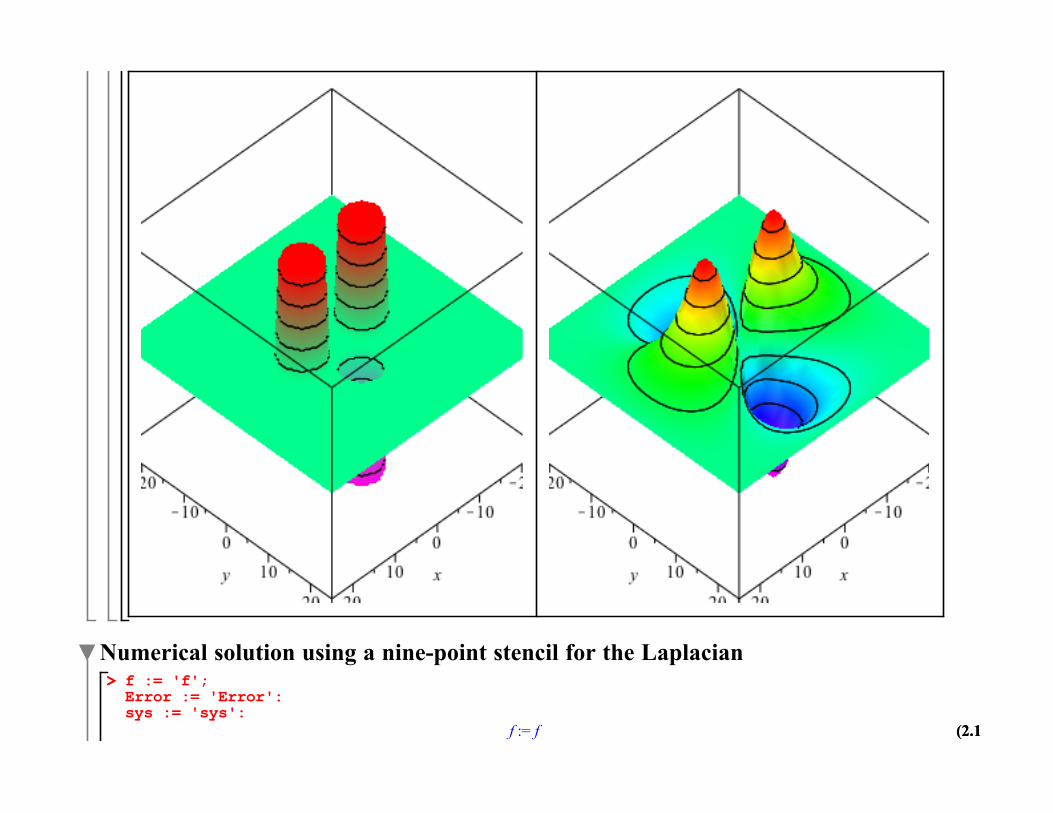
Here is an example problem the calculates the electric potential around a ring of 2n alternating charges. We model the charges as discs of radius r located a distance of R away from the origin and with surface charge density ±1. (For n = 1, this is an electric dipole.)n := 2;r := 4;R := 7;L := 25;g := [x->0,x->0,x->0,x->0];

(1.2.5)(1.2.5)
(1.2.4)(1.2.4)
> >
> >
(1.2.1)(1.2.1)
> >
> >
(1.1.3)(1.1.3)
f := (x,y) -> add((-1)^i*Heaviside(r^2-(x-R*cos(Pi*i/n))^2 - (y-R*sin(Pi*i/n))^2),i=0..2*n-1);p[1] := plot3d(f(x,y),x=-L..L,y=-L..L,grid=[100,100],shading=zhue,axes=boxed,style=patchcontour,labels=[x,y,`f(x,y)`]):p[2] := PoissonSolve(30,f,g,L,1):display(Array([p[1],p[2]]));
n := 2r := 4R := 7L := 25
g := x/0, x/0, x/0, x/0
f := x, y /add K1 i Heaviside r2 K xKR cosp in
2
K yKR sinp in
2
, i = 0 ..2 nK 1
(1.2.5)(1.2.5)
> >
(1.2.4)(1.2.4)
> >
> >
(2.1)(2.1)
(1.2.1)(1.2.1)
> >
> >
(1.1.3)(1.1.3)
Numerical solution using a nine-point stencil for the Laplacianf := 'f';Error := 'Error':sys := 'sys':
f := f

(1.2.5)(1.2.5)
> >
> >
> >
> >
(1.2.1)(1.2.1)
(1.2.4)(1.2.4)
(2.2)(2.2)
> >
> >
(1.1.3)(1.1.3)
We now attempt to find a more accurate stencil to the PDE (1.1). Let us assume a nine point stencil for the Laplacian of the form:substencil[3] := diff(u(x,y),x,x)+diff(u(x,y),y,y) = add(add(a[i,j]/h^2*u(x+i*h,y+j*h),i=-1..1),j=-1..1);stencil[2] := subs(isolate(substencil[3],diff(u(x,y),x,x)),pde);
substencil3 := v2
vx2 u x, y Cv2
vy2 u x, y =aK1, K1 u xK h, yK h
h2 Ca0, K1 u x, yK h
h2 Ca1, K1 u xC h, yK h
h2
CaK1, 0 u xK h, y
h2 Ca0, 0 u x, y
h2 Ca1, 0 u xC h, y
h2 CaK1, 1 u xK h, yC h
h2 Ca0, 1 u x, yC h
h2
Ca1, 1 u xC h, yC h
h2
stencil2 :=aK1, K1 u xK h, yK h
h2 Ca0, K1 u x, yK h
h2 Ca1, K1 u xC h, yK h
h2 CaK1, 0 u xK h, y
h2 Ca0, 0 u x, y
h2
Ca1, 0 u xC h, y
h2 CaK1, 1 u xK h, yC h
h2 Ca0, 1 u x, yC h
h2 Ca1, 1 u xC h, yC h
h2 K f x, y
This stencil involves a square array of points centered about x, y , as shown in the plot:display([seq(seq(polygonplot(ngon(20,i,j,0.1,Pi/2),color=red),i=-1..1),j=-1..1),textplot([seq([i,-0.1,typeset(u(x+i*h,y))],i=-1..1),seq([i,0.9,typeset(u(x,y+h))],i=-1..1),seq([i,-1.1,typeset(u(x,y-h))],i=-1..1)],align={below})],view=[-1.4..1.4,-1.4..1.4],tickmarks=[[-1=x-h,0=x,1=x+h],[-1=y-h,0=y,1=y+h]],axes=boxed,scaling=constrained,labels=["",""],title="Nine point stencil of the Laplacian");

(1.2.5)(1.2.5)
(2.3)(2.3)
(1.2.4)(1.2.4)
> >
> >
> >
(1.2.1)(1.2.1)
> >
> >
(1.1.3)(1.1.3)
u xK h, y u x, y u xC h, y
u x, yC h u x, yC h u x, yC h
u x, yK h u x, yK h u x, yK h
x K h x x C h
y K h
y
y C h
Nine point stencil of the Laplacian
We will now calculate the error in the stencil, simplify the expression using the PDE (1.1), and then select the ai, j coefficients to minimize the error. More specifically, we'll try to eliminate the derivatives of u x, y of order 2 and higher from the Taylor series of (2.2) using the following relations:derivative[1] := isolate(pde,diff(u(x,y),x,x));derivative[2] := diff(derivative[1],x);derivative[3] := diff(derivative[2],x);

(1.2.5)(1.2.5)
> >
> >
> >
(1.2.1)(1.2.1)
(2.3)(2.3)
(1.2.4)(1.2.4)
(2.4)(2.4)
> >
> >
(1.1.3)(1.1.3)
derivative1 := v2
vx2 u x, y = Kv2
vy2 u x, y C f x, y
derivative2 := v3
vx3 u x, y = Kv3
vy2 vx u x, y C
v
vx f x, y
derivative3 := v4
vx4 u x, y = Kv4
vy2 vx2 u x, y Cv2
vx2 f x, y
Here is our calculation of the error in the stencil (2.2). The set sys[Poisson] is the set of equations to be satisfied by the ai, j's to ensure
that the error is O h3 or higher.Error[Poisson] := convert(convert(series(stencil[2],h,5),polynom),diff):Error[Poisson] := dsubs(convert(derivative,list),Error[Poisson]):vars := {seq(seq(a[i,j],i=-1..1),j=-1..1)}:Indets := indets(Error[Poisson]) minus vars minus {x,y};Error[Poisson] := collect(Error[Poisson],Indets,'distributed'):sys[Poisson] := {coeffs(Error[Poisson],Indets)};
Indets := h,v
vx f x, y ,
v
vy f x, y , v2
vx2 f x, y , v2
vy2 f x, y ,v
vx u x, y ,
v
vy u x, y , v2
vy2 u x, y , v3
vy3 u x, y ,
v4
vy4 u x, y , v2
vy vx f x, y , v2
vy vx u x, y , v3
vy2 vx u x, y , f x, y , u x, y
sysPoisson := aK1, K1 K a1, K1 K a
K1, 1 C a1, 1, K16
aK1, 1 C
16
aK1, K1 K
16
a1, K1 C16
a1, 1,12
aK1, 1 K
12
aK1, K1
K12
a1, K1 C12
a1, 1, K12
a1, 0 K12
aK1, 0 C
12
a0, 1 C12
a0, K1, KaK1, K1 C a1, 0 C a1, 1 C a1, K1 K a
K1, 0 K aK1, 1,
K13
aK1, K1 K
16
a1, 0 C13
a1, 1 C16
aK1, 0 K
13
aK1, 1 C
13
a1, K1, K16
aK1, 0 C
16
a1, 0 C16
a1, 1 K16
aK1, 1
K16
aK1, K1 C
16
a1, K1, K124
aK1, 0 K
124
a1, 0 C524
a1, K1 C524
aK1, 1 C
524
aK1, K1 C
524
a1, 1, Ka0, K1 K aK1, K1
K a1, K1 C a0, 1 C a1, 1 C aK1, 1, K
16
a0, K1 K13
aK1, 1 K
13
a1, 1 C13
a1, K1 C16
a0, 1 C13
aK1, K1,
124
a1, 0
C124
a1, K1 C124
aK1, 0 C
124
aK1, 1 C
124
aK1, K1 C
124
a1, 1,12
aK1, 0 K 1C
12
aK1, 1 C
12
aK1, K1 C
12
a1, K1

(1.2.5)(1.2.5)
> >
(2.6)(2.6)
> >
> >
(1.2.1)(1.2.1)
(2.5)(2.5)
(2.3)(2.3)
(2.7)(2.7)
(1.2.4)(1.2.4)
(2.4)(2.4)
> >
> >
> >
> >
(1.1.3)(1.1.3)
C12
a1, 0 C12
a1, 1,124
a1, 0 C124
aK1, 0 C
124
a0, K1 K16
a1, K1 K16
a1, 1 C124
a0, 1 K16
aK1, 1 K
16
aK1, K1,
aK1, K1 C a
K1, 0 C a0, K1 C a1, 1 C a1, K1 C a1, 0 C aK1, 1 C a0, 0 C a0, 1
This a linear system of 14 equations for 9 unknowns; there is no solution.nops(sys[Poisson]);nops(vars);solve(sys[Poisson]);
149
So the stencil (2.2) cannot be made to yield an error smaller that O h2 when solving Poisson's equation. This is no better than the five point stencil of the previous section. However if we now specialize to Laplace's equation by setting f x, y = 0, we can do a little better:Error[laplace] := dsubs(f(x,y)=0,Error[Poisson]):vars := {seq(seq(a[i,j],i=-1..1),j=-1..1)}:Indets := indets(Error[laplace]) minus vars minus {x,y};Error[laplace] := collect(Error[laplace],Indets,'distributed'):sys[laplace] := {coeffs(Error[laplace],Indets)};
Indets := h,v
vx u x, y ,
v
vy u x, y , v2
vy2 u x, y , v3
vy3 u x, y , v4
vy4 u x, y , v2
vy vx u x, y , v3
vy2 vx u x, y , u x, y
syslaplace := aK1, K1 K a1, K1 K a
K1, 1 C a1, 1, K12
a1, 0 K12
aK1, 0 C
12
a0, 1 C12
a0, K1, KaK1, K1 C a1, 0 C a1, 1 C a1, K1
K aK1, 0 K a
K1, 1, K13
aK1, K1 K
16
a1, 0 C13
a1, 1 C16
aK1, 0 K
13
aK1, 1 C
13
a1, K1, Ka0, K1 K aK1, K1 K a1, K1 C a0, 1
C a1, 1 C aK1, 1, K
16
a0, K1 K13
aK1, 1 K
13
a1, 1 C13
a1, K1 C16
a0, 1 C13
aK1, K1,
124
a1, 0 C124
aK1, 0
C124
a0, K1 K16
a1, K1 K16
a1, 1 C124
a0, 1 K16
aK1, 1 K
16
aK1, K1, a
K1, K1 C aK1, 0 C a0, K1 C a1, 1 C a1, K1 C a1, 0
C aK1, 1 C a0, 0 C a0, 1
We now have 8 equations for 9 unknowns, yielding a one parameter family of solutions for the coefficients:nops(sys[laplace]);nops(vars);

(1.2.5)(1.2.5)
> >
> >
> >
> >
(1.2.1)(1.2.1)
> >
(2.8)(2.8)
(2.3)(2.3)
(2.7)(2.7)
(2.9)(2.9)
(1.2.4)(1.2.4)
(2.4)(2.4)
> >
> >
> >
(1.1.3)(1.1.3)
(2.10)(2.10)
solve(sys[laplace]);89
aK1, K1 = a1, 1, a
K1, 0 = 4 a1, 1, aK1, 1 = a1, 1, a0, K1 = 4 a1, 1, a0, 0 = K20 a1, 1, a0, 1 = 4 a1, 1, a1, K1 = a1, 1, a1, 0 = 4 a1, 1, a1, 1
= a1, 1
What is the reason behind the different sizes of sys[Poisson] and sys[laplace]? Basically, there are more indeterminants in the Poisson equation error from the source function (i.e., f x, y , fx x, y , fy x, y , etc.) resulting in more equations that must be satisfied to
cancel all the terms of order h2 or less. The classic nine-point stencil is defined by the following assumption (of course, this is arbitrary and can be changed):assumptions := {a[1,1]=1/6};ans := solve(subs(assumptions,sys[laplace])) union assumptions;
assumptions := a1, 1 =16
ans := aK1, K1 =
16
, aK1, 0 =
23
, aK1, 1 =
16
, a0, K1 =23
, a0, 0 = K103
, a0, 1 =23
, a1, K1 =16
, a1, 0 =23
, a1, 1 =16
We sub this back into (2.2):stencil[2] := subs(ans,stencil[2]);
stencil2 :=16
u xK h, yK h
h2 C23
u x, yK h
h2 C16
u xC h, yK h
h2 C23
u xK h, y
h2 K103
u x, y
h2
C23
u xC h, y
h2 C16
u xK h, yC h
h2 C23
u x, yC h
h2 C16
u xC h, yC h
h2 K f x, y
Note that we have left the source term in this expression; the reason will be apparent shortly. Let's calculate the error with these specific values of the coefficients:Error[poisson] := dsubs(convert(derivative,list),convert(convert(series(stencil[2],h,6),`+`),diff));
Errorpoisson :=112
h2 v2
vy2 f x, y C112
h2 v2
vx2 f x, y CO h4
We immediately see that the leading order term in the error is f h2V2f x, y = h4
V4u x, y so it will indeed vanish for Laplace's equation, and we will have a stencil with error O h4 . But the crucial thing to note is that f x, y is a known function, so we can actually calculate the h2 term in (2.10) explicitly. Hence, it is possible to modify our stencil in such a way as to cancel this error term:

(1.2.5)(1.2.5)
(2.13)(2.13)
(2.11)(2.11)
> >
> >
(1.2.1)(1.2.1)
> >
(2.3)(2.3)
> >
(2.7)(2.7)
(1.2.4)(1.2.4)
(2.4)(2.4)
> >
(2.12)(2.12)
> >
> >
> >
(2.14)(2.14)
(1.1.3)(1.1.3)
> >
stencil[2] := stencil[2]-convert(Error[poisson],polynom);
stencil2 :=16
u xK h, yK h
h2 C23
u x, yK h
h2 C16
u xC h, yK h
h2 C23
u xK h, y
h2 K103
u x, y
h2
C23
u xC h, y
h2 C16
u xK h, yC h
h2 C23
u x, yC h
h2 C16
u xC h, yC h
h2 K f x, y K112
h2 v2
vy2 f x,
y K112
h2 v2
vx2 f x, y
If the source is known analytically, we could in principle calculate the derivatives directly. But the source might not be known analytically (i.e., we could only have numeric knowledge), or we may be coding in an environment where we cannot take the derivative automatically (i.e., in C or FORTRAN). At any rate, we only need the derivatives to enough accuracy to negate the leading order term in (2.10), so we can use the followed centered stencils:substencil[4] := GenerateStencil(diff(f(x,y),x,x),3);substencil[5] := GenerateStencil(diff(f(x,y),y,y),3);
This stencil is of order 2
substencil4 := v2
vx2 f x, y =f xK h, y
h2 K2 f x, y
h2 Cf xC h, y
h2
This stencil is of order 2
substencil5 := v2
vy2 f x, y =f x, yK h
h2 K2 f x, y
h2 Cf x, yC h
h2
Subbing these in to (2.11) yield the final form of the nine-point stencil of the Poisson equation:stencil[2] := expand(subs(substencil[4],substencil[5],stencil[2]));
stencil2 :=16
u xK h, yK h
h2 C23
u x, yK h
h2 C16
u xC h, yK h
h2 C23
u xK h, y
h2 K103
u x, y
h2
C23
u xC h, y
h2 C16
u xK h, yC h
h2 C23
u x, yC h
h2 C16
u xC h, yC h
h2 K23
f x, y K112
f x, yK h
K112
f x, yC h K112
f xK h, y K112
f xC h, y
We confirm that the error in this stencil is of order h4 for the Poisson equation (not just the Laplace equation):Error[poisson] := dsubs(convert(derivative,list),convert(convert(series(stencil[2],h,8),`+`),diff));

(1.2.5)(1.2.5)
(2.11)(2.11)
> >
> >
(1.2.1)(1.2.1)
(2.15)(2.15)
(2.3)(2.3)
> >
(2.7)(2.7)
(1.2.4)(1.2.4)
(2.4)(2.4)
> >
> >
> >
> >
> >
(2.14)(2.14)
(1.1.3)(1.1.3)
Errorpoisson := K1
240 h4 v4
vy4 f x, y C190
h4 v4
vy2 vx2 f x, y K1
240 h4 v4
vx4 f x, y CO h6
Note that even this error is only a functional of f x, y , not of the solution u x, y . Hence, we could have even cancelled this term in the error by adding more terms to (2.13) if an even more accurate stencil is desired. However, the finite difference representation of the higher order derivatives in (2.14) will require more than the nine points already in (2.13), which is not desirable if we cannot take derivatives of f analytically.
The PoissonSolve procedure from above does not need to be modified to use the nine-point stencil (instead of the five-point) as long as we define a mapping Stencil[2] that yields the constraint among the ui, j's at a given lattice point:Subs := seq(seq(u(x+ii*h,y+jj*h)=u[i+ii,j+jj],ii=-1..1),jj=-1..1),seq(seq(f(x+ii*h,y+jj*h)=f[i+ii,j+jj],ii=-1..1),jj=-1..1):stencil[2] := subs(Subs,stencil[2]):Stencil[2] := unapply(stencil[2],h,i,j,u,f);
Stencil2 := h, i, j, u, f /16
ui K 1, j K 1
h2 C23
ui, j K 1
h2 C16
ui C 1, j K 1
h2 C23
ui K 1, j
h2 K103
ui, j
h2 C23
ui C 1, j
h2
C16
ui K 1, j C 1
h2 C23
ui, j C 1
h2 C16
ui C 1, j C 1
h2 K23
fi, j K112
fi, j K 1 K112
fi, j C 1 K112
fi K 1, j K112
fi C 1, j
Here is some example output:n := 2;r := 4;R := 7;L := 25;g := [x->0,x->0,x->0,x->0];f := (x,y) -> add((-1)^i*Heaviside(r^2-(x-R*cos(Pi*i/n))^2 - (y-R*sin(Pi*i/n))^2),i=0..2*n-1);p[1] := plot3d(f(x,y),x=-L..L,y=-L..L,grid=[100,100],shading=zhue,axes=boxed,style=patchcontour,labels=[x,y,`f(x,y)`]):p[2] := FivePoint(30,f,g,L,2):display(Array([p[1],p[2]]));
n := 2r := 4R := 7L := 25

(1.2.5)(1.2.5)
(2.11)(2.11)
> >
> >
(1.2.1)(1.2.1)
(2.3)(2.3)
> >
(2.7)(2.7)
(1.2.4)(1.2.4)
(2.4)(2.4)
> >
> >
> >
(2.14)(2.14)
(1.1.3)(1.1.3)
g := x/0, x/0, x/0, x/0
f := x, y /add K1 i Heaviside r2 K xKR cosp in
2
K yKR sinp in
2
, i = 0 ..2 nK 1