Vasilis Friderikos and Katerina PapadakiInterference aware routing for minimum frame length schedules in wireless mesh networks Journal article

Original citation: Friderikos, Vasilis and Papadaki, Katerina (2008) Interference aware routing for minimum frame length schedules in wireless mesh networks. EURASIP journal on wireless communications and networking, article ID 817876 DOI: 10.1155/2008/817876 This version available at: http://eprints.lse.ac.uk/26208/ Available in LSE Research Online: December 2009 © 2008 Vasilis Friderikos and Katerina Papadaki. This is an open access article distributed under the Creative Commons Attribution License, which permits unrestricted use, distribution, and reproduction in any medium, provided the original work is properly cited.

LSE has developed LSE Research Online so that users may access research output of the School. Copyright © and Moral Rights for the papers on this site are retained by the individual authors and/or other copyright owners. Users may download and/or print one copy of any article(s) in LSE Research Online to facilitate their private study or for non-commercial research. You may not engage in further distribution of the material or use it for any profit-making activities or any commercial gain. You may freely distribute the URL (http://eprints.lse.ac.uk) of the LSE Research Online website.

Hindawi Publishing CorporationEURASIP Journal on Wireless Communications and NetworkingVolume 2008, Article ID 817876, 13 pagesdoi:10.1155/2008/817876

Research ArticleInterference Aware Routing for Minimum Frame LengthSchedules in Wireless Mesh Networks

Vasilis Friderikos1 and Katerina Papadaki2

1 Division of Engineering, Centre for Telecommunications Research, King’s College London, Strand,London WC2R 2LS, England, UK

2 Department of Management, Operational Research Group, London School of Economics, Houghton Street,London WC2A 2AE, England, UK

Correspondence should be addressed to Katerina Papadaki, k.p.papadaki@lse.ac.uk

Received 18 January 2008; Revised 4 June 2008; Accepted 15 August 2008

Recommended by Athanasios Vasilakos

The focus of this paper is on routing in wireless mesh networks (WMNs) that results in spatial TDMA (STDMA) scheduleswith minimum frame length. In particular, the emphasis is on spanning tree construction; and we formulate the joint routing,power control, and scheduling problem as a mixedinteger linear program (MILP). Since this is an N P -complete problem, wepropose a low-complexity iterative pruning-based routing scheme that utilizes scheduling information to construct the spanningtree. A randomized version of this scheme is also discussed and numerical investigations reveal that the proposed iterative pruningalgorithms outperform previously proposed routing schemes that aim to minimize the transmitted power or interference producedin the network without explicitly taking into account scheduling decisions.

Copyright © 2008 V. Friderikos and K. Papadaki. This is an open access article distributed under the Creative CommonsAttribution License, which permits unrestricted use, distribution, and reproduction in any medium, provided the original work isproperly cited.

1. INTRODUCTION

Algorithmic aspects of wireless mesh networks (WMNs)are currently a vigorous area of research and have steadilyaccumulated momentum over the last few years. The lead-ing exponents of this increased interest are the potentialmultifarious applications of WMNs [1]. Admittedly, the twomost important of them are provision of low-cost and rapid-deployable broadband last mile connectivity to the Internetor backhaul support for 3G cells and IEEE 802.11“x” hotspots.

Efficient resource utilization in WMNs calls for schedul-ing and routing policies that maximize the aggregatethroughput of the system. Under this perspective, the centraltheme of this paper is the design of joint scheduling andshortest-path spanning tree schemes that provide increasedsystem performance. With a preconstructed spanning treewithin the mesh network, the cornerstone aim of thescheduling engine is either to maximize the transmissionopportunities of active links in a specific time window (framelength) by taking into account the interference caused by

simultaneously transmitting nodes or to minimize the timespan for all links to transmit, that is, minimize frame length.Concurrent transmissions are of utmost importance sincethey increase system efficiency but can lead to erroneousreception at the receiver if the level of the received signalis too weak compared to the aggregate interference. Thus,the spatial reuse of timeslots heavily depends on the selectedactive set of links in the mesh topology; but, the active setof links is constructed by the routing algorithm. Therefore,and as it will become vividly clear in the sequel, thereis an interplay between scheduling and routing decisions.The rationale of designing joint routing and schedulingschemes stems exactly from this interplay between the twofunctionalities.

The medium-access control scheme considered hereafteris based on time division multiple access (TDMA), wheretime is divided into timeslots and each node can transmitonly at predefined timeslots, thus, collisions can be avoided(the same analysis can also be applied for FDMA-basednetworks). Since nodes are spatially distributed, timeslotscan be potentially reused by nodes that are sufficiently far

2 EURASIP Journal on Wireless Communications and Networking

apart. Spatial reusing of timeslots has been defined in theseminal work of Nelson and Kleinrock [2] and is calledspatial TDMA (STDMA).

In this paper, we focus on utilizing shortest-path algo-rithms, which are widely studied and used in practise. Theemphasis is on Dijkstra’s algorithm which for boundeddegree graphs finds the shortest paths from a source nodeto every other node in O(n logn) time, where n is thenumber of nodes in the network. The cost metric used is therequired transmission power for a link (i, j) to be established.We focus on rooted spanning tree construction (for bothuplink and downlink) since the mesh mode specificationsthat have been integrated into the IEEE 802.16-2004 standardare based on tree topology. Our proposed pruning schemesrun Dijkstra iteratively, and at each iteration, eliminate(prune) links that produce high interference; the resultingtree’s scheduling performance is evaluated by using optimalscheduling or a greedy scheduling heuristic and the tree withthe best scheduling performance is kept. Thus, schedulinginformation is incorporated in making decisions aboutrouting.

We compare the proposed pruning algorithm with otherDijkstra-based schemes. These heuristics use as costs linearcombinations of the required power for transmission andthe interference produced. We show that proposed pruningalgorithm outperforms these heuristics.

The rest of the paper is organized as follows. InSection 2, selected closely related previous works in the areaof joint routing and scheduling are outlined. The problemdescription and the mixed-integer linear program (MILP)formulation are detailed in Section 3. The inherent interplaybetween routing and scheduling is explained in Section 4. InSection 5, suboptimal joint scheduling and routing schemesare explained; and Section 6 outlines the two flavors ofthe proposed pruning algorithm. Numerical investigationsare reported in Section 7; and finally, Section 8 concludesthe paper by outlining the main findings followed by briefremarks on future avenues for research.

2. REVIEW OF SELECTED PRIOR WORKS

After the introduction of the spatial TDMA concept byNelson and Kleinrock in [2], general timeslot (or channel)assignment scheduling problems have been extensively stud-ied in the literature. The bulk of previous research workfocused on graph theoretic solutions by conceiving linkscheduling as a graph-coloring problem [3–5]. In the basicsetting, graph-coloring approaches aim to tackle the primaryand secondary conflicts between links. More specifically, anypair of directed edges (a, b), (c,d) may be colored withthe same color if and only if (i) a, b, c,d are all mutuallydistinct and (ii) edges (a,d), (c, b) do not belong in the setof edges in the graph. When the first (second) condition failsto hold, then there will be a primary (secondary) conflictbetween edges (a, b) and (c,d). Scheduling based on graphtheoretic tools proved essential for formally defining theproblem and for the design of distributed solutions. Thelimitations on the other hand of these solutions stem fromthe fact that the aggregate effect of interference of links

transmitting in concurrent timeslots (reflected in the signal-to-interference noise ratio (SINR)) is not taken explicitly intoaccount [6]. Hence, a schedule provided by a graph-coloringtechnique may lead to an infeasible allocation when the SINRthresholds are taken into account. Related to this last pointis the observation that an optimal schedule based on graphcoloring can be considered as a lower bound of the minimumnumber of timeslots that can be used in the network.

To fill this void, the authors in [7] have explicitly takeninto account the SINR thresholds together with powercontrol for constructing minimum frame length schedulingin STDMA networks with directional antennas. From acomputational complexity perspective, even without takinginto account the aggregate interference, constructing a trans-mission schedule of timeslots where all links are scheduledwith the minimum number of timeslots (i.e., minimumframe length) has shown to be an N P -complete problem[8].

The work of Tassiulas and Ephremides [9] showed thatthe capacity region of wireless multihop networks dependson the power allocation vector (which itself depends onchannel conditions) as well as the routing and schedulingdecisions. This formal characterization of the inherentcoupling between power control, scheduling, and routing,sparked a research interest in schemes that attempt tooptimize them jointly [10, 11]. These so-called cross-layeroptimization approaches have recently been extended totake into account end-to-end flow and congestion controldecisions (transport layer) [12]. Polynomial complexityalgorithms together with necessary and sufficient conditionsfor optimal scheduling and routing of a predefined setof source-destination rates in mesh networks have beendiscussed in [13]. In contrast to these previous works, theemphasis in this paper is on how to construct spanningtrees that minimize the frame length (in terms of requiredtimeslots) in the mesh network.

Finally, it is worth mentioning that pruning techniqueshave been mainly used within quality of service (QoS)routing to produce a sparser graph, consisting entirely offeasible links [14, 15]. In these QoS routing schemes, linksare deleted from the topology if their available resourcesdo not meet the corresponding constraints. In our case,the incentive for link pruning is a rather different one;pruning is used to delete links that produce high interferenceto neighbor nodes that can lead to low-spatial reuse oftimeslots.

2.1. Contribution of the paper

To the authors best knowledge, this is the first paper thatexplicitly addresses the issue of how to jointly construct aspanning tree while minimizing the required frame length(in terms of the number of timeslots) in a wireless meshnetwork. In that respect, the contributions of the paperrepresent measurable progress on the following fronts:

(1) formulation of MILP to perform optimal jointlyspanning tree construction and scheduling that min-imizes the required frame length in timeslots;

V. Friderikos and K. Papadaki 3

(2) interference aware iterative pruning routing algo-rithms to construct spanning trees in the WMN witha minimum frame length schedule;

(3) quantification of the gains in terms of schedulingof the pruning schemes compared to previouslyproposed schemes based on an extensive set ofsimulations.

It is worth mentioning that even though in this paper we haveassumed omnidirectional antennas (0 dB gain) and baselinepath loss models, the proposed scheme is independent of theoperational characteristics and models used. Thus, resultsdrawn in this paper can be applied for different antennaradiation patterns and/or link gain models.

3. PROBLEM DESCRIPTION

Before embarking our study of suboptimal solutions inlater sections, we first formulate the problem of jointrouting and scheduling as an MILP. Section 3.1 deals withthe mathematical programming formulation for performingSTDMA scheduling under the assumption of a predefinedroute and Section 3.2 augments the scheduling model toincorporate routing decisions.

For performing joint scheduling and routing in WMNs,we consider the graph G, defined by the (V ,L) pair, whereV is a set of vertices (wireless nodes) and L is the set oftransmission links that satisfy the SINR threshold criterion,

L = {(u, v) | u, v ∈ V s.t. u /=v can transmit to v

and vice versa}.

(1)

Routing is usually performed using a weighting functionw : L→R, which assigns a weight to each edge. The weight ofan edge is commonly related with the required transmissionpower, which depends on the Euclidean distance betweenthe nodes and the level of interference. A number ofdifferent possible edge weights that implicitly take intoaccount scheduling information for suboptimal routing andscheduling will be discussed in the following sections.

3.1. A mixed-integer linear programming (MILP)formulation for scheduling

We first focus our attention on how to perform optimalscheduling decisions under the assumption that routingpaths are preconstructed. Similar formulations appear in[16, 17]. In this case, the routing will create the directedgraph GS = (V ,LS), where LS ⊆ L, and scheduling will beperformed on GS.

We encapsulate power control within the MILP formu-lation by introducing the variable pi jt, which expresses thetransmitted power by node i in link (i, j) at timeslot t,under the constraint that 0 ≤ pi jt ≤ Pmax for all t. Thevariable Pmaxexpresses the power ceiling at the transmittingnode (without loss of generality Pmax is assumed to be equalfor all nodes in the WMN). Additionally, we assume thatomnidirectional antennas are used by all wireless nodes totransmit and receive signals. Thus, the interference level

produced by link (i, j) to all other receiving nodes willbe based on their Euclidean distance with node i. Witha constant target bit error rate (i.e., Eb/N0 = Γ), thetransmission can be translated into a signal-to-interferenceratio requirement, which will be denoted hereafter as γ. ByW we denote the lump sum thermal noise power, and by gi jthe link gain between nodes i, j which encapsulates both pathloss and slow fading.

To be able to express now the problem in a mathematicalprogramming setting, we introduce the boolean variables xi jtand πt , which are defined as follows:

xi jt =⎧⎨

⎩

1, if link (i, j) active at timeslot t,

0, otherwise,

πt =⎧⎨

⎩

1, if timeslot t is used,

0, otherwise.

(2)

The mixed-integer linear program for scheduling that mini-mizes the required frame length in a predefined route on theset of links LS is denoted as OS (LS) and can be written asfollows:

minM∑

t=1

πt, (3)

∑

(i, j)∈LSxi jt ≤ πt·|LS| ∀t, (4)

M∑

t=1

xi jt ≥ 1 ∀(i, j) ∈ LS, (5)

∑

j:(i, j)∈LSxi jt +

∑

k:(k,i)∈LSxkit ≤ 1 ∀i ∈ V , ∀t, (6)

gi j pi jt +(1− xi jt

)Λ

∑(m,n)∈LS\{(i, j)}gmj pmnt +W

≥ γ ∀(i, j) ∈ LS, ∀t, (7)

xi jt ≤pi jtgi jWγ

∀(i, j) ∈ LS, ∀t, (8)

xi jt ≥ pi jt/Pmax ∀(i, j) ∈ LS, ∀t, (9)

xi jt ∈ {0, 1} ∀(i, j) ∈ LS, ∀t, (10)

πt ∈ {0, 1} ∀t, (11)

0 ≤ pi jt ≤ Pmax ∀(i, j) ∈ LS, ∀t. (12)

In this formulation, an initial frame lengthM is assumed,where all links can be easily scheduled. For example, an initialframe length value M could be the number of links.

Constraints (4) are the binding constraints for variablesπt and xi jt. The requirement that all links transmit at leastonce during the frame length is ensured by constraint (5).Constraint (6) is the degree constraint, that is, a nodecannot transmit and receive at the same timeslot. Constraint(7) expresses the required SINR threshold that should besatisfied in order to have a successful reception at thereceiver. The term Λ(1 − xi jt) ensures that the inequality issatisfied when link (i, j) does not transmit at timeslot t, fora sufficiently high value of Λ. The binding constraints for

4 EURASIP Journal on Wireless Communications and Networking

variables xi jt and pi jt are shown in (8) and (9). These bindingconstraints ensure that if link (i, j) is not transmitting attimeslot t, then the transmitted power pi jt is zero and viceversa. Constraint (8) is based on the assumption that alllinks (i, j) in LS satisfy the SINR constraint when there areno concurrent transmissions, which is equivalent to gi j pi jt >γW .

3.2. Performing joint scheduling and routing

In the previous section, we formulated the schedulingproblem given a fixed routing LS. Allowing flexibility withrouting decisions can improve the resulting scheduling. Theaim here is to construct a routing such that the number oftimeslots in a time frame is minimized. We focus our routingdecisions on constructing spanning trees. The direction ofthe spanning tree depends on whether we are performinguplink or downlink transmission.

We augment the previously defined scheduling model toincorporate both routing (tree construction) and schedulingdecisions. Note that the optimal joint routing and schedulingproblem operate on the graph G = (V ,L). Before describingthe new constraints that need to be added, we first introducethe routing variables yi, j , which are defined as follows:

yi j =⎧⎨

⎩

1, link (i, j) in optimal spanning tree,

0, otherwise.(13)

Without loss of generality, we assume that node r is the rootnode in the constructed spanning tree. Based on the abovedefinitions, the optimal joint scheduling and spanning treeconstruction problem will be denoted as OSR (L), which isbased on the set of all feasible links L. The mathematicalformulation of the OSR (L) can be constructed by adding thefollowing routing constraints to the already defined OS (L)formulation:

yi j ≤M∑

t=1

xi jt ≤ yi j·M ∀(i, j) ∈ L, (14)

∑

(i, j)∈L:i, j∈Dyi j ≤ |D| − 1 ∀D ⊆ V , (15)

∑

(i, j)∈Lyi j = |V | − 1 ∀(i, j) ∈ L, (16)

∑

j∈V :(i, j)∈Lyi j = 1 ∀i ∈ V \ {r},

∑

(r,i)∈Lyri = 0, (17)

yi j + yji ≤ 1 ∀(i, j) ∈ L. (18)

Constraint (14) binds the boolean variables xi jt and yi jso that a link (i, j) transmits if and only if it belongs to theoptimal spanning tree. Constraint (15) ensure that there areno cycles and constraint (16) ensure that there are |V | − 1links. Since an acyclic graph with |V | nodes and |V |−1 edgesis a spanning tree, the previous two constraints constructa spanning tree. Constraints (17), (18) ensure that the treeis directed in the uplink direction towards root node r. In

A1

A2

A3

A4

Root node

Figure 1: Worst-case scenario for timeslot reuse: the number ofrequired timeslots is equal to the number of edges (i.e., M = |L|).

the case of downlink, constraint (17) are replaced by thefollowing:

∑

j∈V :( j,i)∈Ly ji = 1 ∀i ∈ V \ {r},

∑

(i,r)∈Lyir = 0. (19)

The OSR (L) formulation constructs a tree that producesschedules with the minimal timeslot frame length. Giventhat OR (LS) is an N P -complete problem [8], the N P -completeness of OSR (L) follows.

4. THE BINDING NATURE OF SPANNING TREECONSTRUCTION AND SCHEDULING

The aim of this section is twofold. Firstly, to reveal the closelycoupled nature of the spanning tree construction and thescheduling problem by focusing on the uplink transmissionproblem. Secondly, this discussion will motivate the pro-posed scheme with polynomial computational complexityfor spanning tree construction.

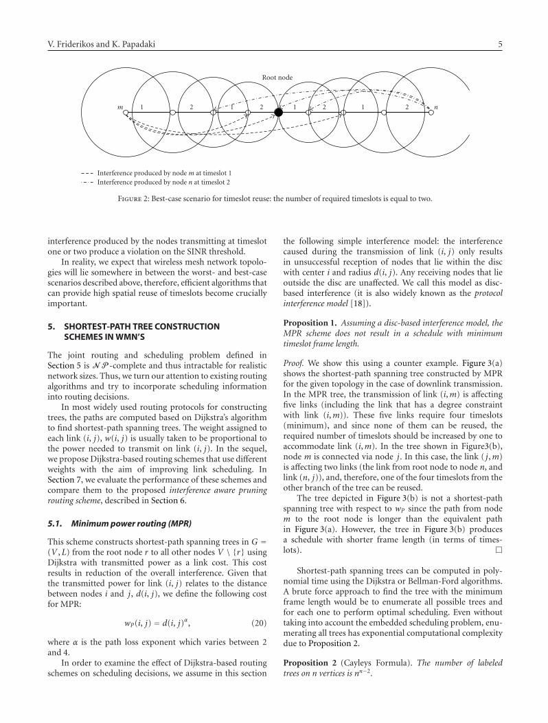
Figure 1 shows the worst-case scenario of a minimumpower spanning tree in terms of utilization of the timeslots.As shown in the figure, the transmission areas of the nodesare nested in the sense that each node’s transmission areaincludes all nodes that are further away from the root node.If we define the transmission area of node i as Ai, then nodes{i, i + 1, i + 2 . . .} fall within the area Ai. This means thateach node i cannot transmit at the same timeslot as nodesi+1, i+2, . . .. Thus, no concurrent transmission can occur andthe number of timeslots required for all nodes to transmitgrows linearly, Ω(n) with the number of transmitting nodes.On the other hand, Figure 2 depicts a topology where theminimum power spanning tree requires only two timeslotsfor all the nodes to transmit. Two timeslots is the minimumnumber required since the degree of the topology is two.As shown in the figure, two timeslots are sufficient sincethe transmission areas of nodes transmitting at timeslot one(or two) do not overlap. Note that this one-dimensionaltopology has the minimum interference between nodes thattransmit concurrently at timeslots one or two and, in thiscase, a new timeslot will only be required if the aggregate

V. Friderikos and K. Papadaki 5

m 1 2 1 2 1 2 1 2 n

Root node

Interference produced by node m at timeslot 1Interference produced by node n at timeslot 2

Figure 2: Best-case scenario for timeslot reuse: the number of required timeslots is equal to two.

interference produced by the nodes transmitting at timeslotone or two produce a violation on the SINR threshold.

In reality, we expect that wireless mesh network topolo-gies will lie somewhere in between the worst- and best-casescenarios described above, therefore, efficient algorithms thatcan provide high spatial reuse of timeslots become cruciallyimportant.

5. SHORTEST-PATH TREE CONSTRUCTIONSCHEMES IN WMN’S

The joint routing and scheduling problem defined inSection 5 is N P -complete and thus intractable for realisticnetwork sizes. Thus, we turn our attention to existing routingalgorithms and try to incorporate scheduling informationinto routing decisions.

In most widely used routing protocols for constructingtrees, the paths are computed based on Dijkstra’s algorithmto find shortest-path spanning trees. The weight assigned toeach link (i, j), w(i, j) is usually taken to be proportional tothe power needed to transmit on link (i, j). In the sequel,we propose Dijkstra-based routing schemes that use differentweights with the aim of improving link scheduling. InSection 7, we evaluate the performance of these schemes andcompare them to the proposed interference aware pruningrouting scheme, described in Section 6.

5.1. Minimum power routing (MPR)

This scheme constructs shortest-path spanning trees in G =(V ,L) from the root node r to all other nodes V \ {r} usingDijkstra with transmitted power as a link cost. This costresults in reduction of the overall interference. Given thatthe transmitted power for link (i, j) relates to the distancebetween nodes i and j, d(i, j), we define the following costfor MPR:

wP(i, j) = d(i, j)α, (20)

where α is the path loss exponent which varies between 2and 4.

In order to examine the effect of Dijkstra-based routingschemes on scheduling decisions, we assume in this section

the following simple interference model: the interferencecaused during the transmission of link (i, j) only resultsin unsuccessful reception of nodes that lie within the discwith center i and radius d(i, j). Any receiving nodes that lieoutside the disc are unaffected. We call this model as disc-based interference (it is also widely known as the protocolinterference model [18]).

Proposition 1. Assuming a disc-based interference model, theMPR scheme does not result in a schedule with minimumtimeslot frame length.

Proof. We show this using a counter example. Figure 3(a)shows the shortest-path spanning tree constructed by MPRfor the given topology in the case of downlink transmission.In the MPR tree, the transmission of link (i,m) is affectingfive links (including the link that has a degree constraintwith link (i,m)). These five links require four timeslots(minimum), and since none of them can be reused, therequired number of timeslots should be increased by one toaccommodate link (i,m). In the tree shown in Figure3(b),node m is connected via node j. In this case, the link ( j,m)is affecting two links (the link from root node to node n, andlink (n, j)), and, therefore, one of the four timeslots from theother branch of the tree can be reused.

The tree depicted in Figure 3(b) is not a shortest-pathspanning tree with respect to wP since the path from nodem to the root node is longer than the equivalent pathin Figure 3(a). However, the tree in Figure 3(b) producesa schedule with shorter frame length (in terms of times-lots).

Shortest-path spanning trees can be computed in poly-nomial time using the Dijkstra or Bellman-Ford algorithms.A brute force approach to find the tree with the minimumframe length would be to enumerate all possible trees andfor each one to perform optimal scheduling. Even withouttaking into account the embedded scheduling problem, enu-merating all trees has exponential computational complexitydue to Proposition 2.

Proposition 2 (Cayleys Formula). The number of labeledtrees on n vertices is nn−2.

6 EURASIP Journal on Wireless Communications and Networking

12

32

4 2

5

3

n

j

m

id1

Root node

(a)

1 2

32

42

3

4

n

j

m

id2

Root node

(b)

Figure 3: (a) Minimum power spanning tree (MPST), and (b) aspanning tree that requires less number of timeslots (better spatialreuse). Timeslots are shown within the rectangular boxes.

5.2. Minimum nearest neighborhoods routing—MNR

The MNR algorithm tries to minimize the number of nodesthat are within the area of each link in the shortest-pathspanning tree. In order to compute such a tree, Dijkstra’salgorithm can be deployed where the cost of each link (i, j) ∈L is equal to the number of receiving nodes that are within itstransmission range (taken to be the disc of center i and radiusd(i, j)). In this case, the cost can be written as follows:

wN (i, j) =∑

n∈V\{i, j,r}I(i, j)(n), (21)

where I(i, j)(n) is the indicator function which is defined asfollows for n /= i, j:

I(i, j)(n) =⎧⎨

⎩

1, if d(i,n) ≤ d(i, j),

0, otherwise.(22)

This algorithm can also include a lower bound on thenumber of nodes that are within the transmission range ofeach link so that connectivity can be established with highprobability [19].

a

b

c

d

Figure 4: Possible edge crossing in the minimum nearest neighbor-hoods spanning tree algorithm.

A drawback of this scheme is that it may introduce edgecrossings in the constructed tree.

Proposition 3. The MNR scheme may create shortest-pathspanning trees that are nonplanar graphs.

Proof. Figure 4 shows a possible construction of a spanningtree based on the MNR algorithm. The root node is node aand after the construction of links (a, b), which has cost 0,and (a, c), which has cost 1, the cost of the link (b,d) is 4(nodes within the circle shown by solid lines) whilst the costfor links (a,d) and (c,d) is 5 and 7, respectively (nodes withinthe dashed and doted dashed circles, resp.). Thus, the least-cost path to node d is through node b and, therefore, an edgecrossing will be introduced.

Link crossing can be detected, and, subsequently, pla-narity can be restored, but the current proposed techniquesneed to be adapted before being applied for tree construction(see [20] and references therein).

5.3. Interference based routing—IR

In this case, the actual interference that will be producedto the other receiving nodes in the network is taken intoaccount to produce the cost for every link in the network.More specifically, the cost for link (i, j) is computed asfollows:

wI(i, j) =∑

n∈V\{i, j,r}g(i,n)

g(i, j). (23)

Therefore, the cost for link (i, j) is inversely proportional tothe link gain g(i, j) but weighted with the aggregate link gainsof node i to all other receiving nodes in the network. Thus,the actual interference that will be produced by link (i, j) isexplicitly taken into account.

5.4. Weighted power and interference routing (WPIR)

In WPIR, the two different metrics (i.e., required power forestablishing the link and interference caused by the link) are

V. Friderikos and K. Papadaki 7

condensed into a single metric via a linear combination. Thecost for link (i, j) can be, therefore, written as follows:

wPI(i, j) = βwP(i, j)Θ + (1− β)wI(i, j), (24)

where β controls the weight of each individual metric inthe cost and Θ is a normalizing constant between theaverage wP and wI values. By this linear combination, asingle weight is assigned to every link and thus it becomespossible to use a Dijkstra-like algorithm. Since differentspanning trees will be constructed with different values of β,a drawback of this scheme is that by linearly combining thetwo metrics, the optimal weighting value will be different fordifferent topologies. This routing scheme is similar to the onediscussed in [21].

6. INTERFERENCE AWARE PRUNING ROUTINGALGORITHM—IAPR

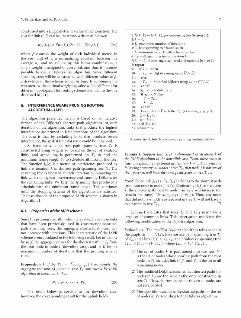
The algorithm presented herein is based on an iterativeversion of the Dijkstra’s shortest-path algorithm. At eachiteration of the algorithm, links that produce the highestinterference are pruned in later iterations of the algorithm.The idea is that by excluding links that produce severeinterference, the spatial timeslot reuse could be enhanced.

At iteration k, a shortest-path spanning tree Tk isconstructed using weights wP based on the set of availablelinks, and scheduling is performed on Tk to find theminimum frame length Sk to schedule all links in the tree.The function Ik(e) is a metric of interference produced bylink e at iteration k in shortest-path spanning tree Tk . Thespanning tree is updated at each iteration by removing thelink with the highest interference and running Dijkstra onthe remaining links. We keep the spanning that produced aschedule with the minimum frame length. This continuesuntil the stopping criteria of the algorithm are satisfied.The pseudocode of the proposed IAPR scheme is shown inAlgorithm 1.

6.1. Properties of the IAPR scheme

Since the pruning algorithm eliminates at each iteration linksthat have been previously used in constructing shortest-path spanning trees, the aggregate shortest-path cost willnot decrease with iterations. This characteristic of the IAPRscheme is encapsulated in the following result. Let us denoteby pk(i) the aggregate power for the shortest path in Tk fromthe root node to node i (downlink case), and let K be themaximum number of iterations that the pruning schemeruns.

Proposition 4. If by Pk = ∑i∈V\{r}pk(i) we denote the

aggregate transmitted power in tree Tk constructed by IAPRalgorithm at iterations k, then

P1 ≤ P2 ≤ · · · ≤ PK . (25)

The result below is specific to the downlink case,however, the corresponding result for the uplink holds.

1: G(V ,L)← G(V ,L), pre-processing (see Section 6.2)2: k ← 0,3: K , maximum number of iterations4: T , best spanning tree found so far5: S, minimum frame length achieved so far6: Tk ← ∅, spanning tree at iteration k7: Sk = |L|, frame length achieved at iteration k by tree Tk8: repeat9: if k = 0 then10: Tk+1 ← Dijkstra using wP on G(V ,L)11: else12: Tk+1 ←Modified Dijkstra using wP on G(V ,L)13: end if14: Sk+1 ← Schedule(Tk+1)15: if Sk+1 < S then16: T ← Tk+1

17: S← Sk+1

18: end if19: Find link e ∈ L such that Ik+1(e) = maxl∈L{Ik+1(l)}20: L← L \ {e}21: k ← k + 122: until (k > K)23: return T , S

Algorithm 1: Interference aware pruning routing (IAPR).

Lemma 1. Suppose link (i, j) is eliminated at iteration k ofthe IAPR algorithm in the downlink case. Then, there exists atleast one spanning tree found at iteration k + 1, Tk+1 with thefollowing property: all nodes of tree Tk, that node j is not one oftheir parents, will have the same predecessor in tree Tk+1.

Proof. Since link (i, j) ∈ Tk , (i, j) belongs to the shortest pathfrom root node to node j in Tk. Eliminating (i, j) at iterationk, the shortest-path cost to node j in Tk+1 will increase (orremain the same). Thus, pk+1( j) ≥ pk( j). Thus, any nodethat did not have node j as a parent in tree Tk will not have jas a parent in tree Tk+1.

Lemma 1 indicates that trees Tk and Tk+1 may have alarge set of common links. This observation motivates thefollowing modification of the Dijkstra algorithm.

Definition 1. The modified Dijkstra algorithm takes as inputthe graph Gk = (V ,Lk), the shortest-path spanning tree Tkof Gk, and a link (i, j) ∈ Tk,Lk, and produces a spanning treeTk+1 of Gk+1 = (V ,Lk+1), where Lk+1 = Lk \ {(i, j)}.

(1) The set of nodes V is partitioned into two sets: V1

is the set of nodes whose shortest path from the rootnode on Tk includes link (i, j), and V2 is the set of allremaining nodes.

(2) The modified Dijkstra assumes that shortest paths fornodes in V2 are the same as the ones constructed intree Tk. Thus, shortest paths for this set of nodes arenot recalculated.

(3) The algorithm calculates the shortest paths for the setof nodes in V1 according to the Dijkstra algorithm.

8 EURASIP Journal on Wireless Communications and Networking

Proposition 5. The tree produced by the modified Dijkstraalgorithm is a shortest-path spanning tree.

Proof. The proof follows from Lemma 1.

The above modification of the Dijkstra algorithm is usedto accelerate the updating of trees in the IAPR scheme atiterations k ≥ 1.

6.2. Preprocessing on the initial graph

In order to accelerate the performance of the algorithm, thefollowing preprocessing step can be implemented. In graphG(V ,L) of WMN, the set L of links is reduced by consideringonly links (i, j) that havewN (i, j) ≤ Nmax (i.e., only links withless than Nmax neighbors are considered) (see Section 5.2).

6.3. Complexity of IAPR

The computational complexity that pertains one iterationof the algorithm is that of the modified Dijkstra algorithm,the pruning operation, and the scheduling engine. Assuminga greedy packing heuristic for scheduling (see Section 7),the complexity of each aforementioned step in one iterationis O(n logn). In the worst-case scenario, the algorithmterminates after K iterations, thus the complexity of theoverall computational can be O(Kn logn) steps.

6.4. Stopping criterion

In general, a stopping criterion is needed to avoid pruninglinks that are required to ensure connectivity. A possiblestopping criterion could be to hault the algorithm at theiteration at which the remaining links no longer can ensurea connected graph. This would mean that we run thealgorithm in the order of |V |2 iterations, in the case of densenetworks, that is, complete graphs. However, in practiseafter the removal of a few high interference links at thebeginning, the algorithm will stop improving. Even thoughthe algorithm will not deteriorate after many iterations (sincewe keep the best schedule), it will be unnecessary to runit until the graph is disconnected. This is intuitive and wehave also verified it experimentally as will be shown in latersections. Thus, either a relatively small number of iterationsshould be chosen or the algorithm should run within somepredefined small time limit. An operator, for example, canput a maximum time limit on the computational time forrunning the routing algorithm. In that case, the number ofiterations will be limited by this time limit.

6.5. A randomized version of the IAPR

At each iteration of the IAPR scheme, the link that producesthe highest interference is pruned with probability one,irrespectively of whether the framelength is decreased or not.A variation of the scheme could be to check a number oflinks ordered by the level of interference they produce, andprune the first link whose removal improves the framelength.In this case, a number of pruning options are considered

and the scheme proceeds in the direction that improves theframelength. However, in the case that none of the V − 1links of the shortest-path tree (when pruned) improve theframelength, the above scheme will be unable to searchfurther and thus stall. In order to further increase the searchspace and at the same time avoid stalling, we randomize theabove scheme by pruning a link with a small probabilityp, even though the resulting frame length produced byremoving this link is not leading to an improvement.The pseudocode of the randomized version of the IAPRscheme (R-IAPR) is shown in Algorithm 2. In the worst-case scenario, the algorithm in each iteration will test alllinks in the shortest-path tree. Therefore, the computationalcomplexity of the R-IAPR scheme can be O(K(V−1)n logn)steps.

7. NUMERICAL INVESTIGATIONS

In this section, we evaluate the performance of the proposedIAPR scheme (both the deterministic and randomized one)compared to the MPR, MNR, IR, and WPIR schemesthat have been detailed in Section 5. Simulations are con-ducted on different randomly generated WMN topolo-gies. For all different schemes, a simple greedy heuristicfor evaluating the scheduling has been used, which isdescribed in Algorithm 3. We denote by S the frame lengthachieved by either the optimal scheduling or the packingheuristic.

The packing heuristic tries to pack as many links aspossible in each time slot that have not yet transmitted inprevious time slots (list A), giving priority to the ones withthe highest transmitted power. This continues until all linkshave transmitted at least once (list A is empty). This packingheuristic is similar to a heuristic used in [16, 22, 23], where itwas shown to produce satisfactory solutions.

The IAPR (and R-IAPR) scheme uses the packingheuristic at each iteration to evaluate the scheduling ofthe current shortest path spanning tree. Further, we usethe following function to evaluate the interference causedby each link (i, j) in the shortest-path spanning tree Tk:Ik((i, j)) = wN (i, j), that is, the number of receiving nodesthat are within the disc with center i and radius d(i, j).

For the WPIR scheme, the value of Θ has been selectedto normalize the average power weight wP and the averageinterference weight wI . The value of β = 0.5, which givesequal weight to the two metrics, has been used in thesimulations.

For the numerical investigations reported in the fol-lowing sections the parameterization of the simulationenvironment is as follows. The path loss model for link (i, j)is PLd(i, j) = PL (do) + 10 η log10(d(i, j)/do), where d(i, j)is the distance of link (i, j), PL (do) is the close in distanceloss (40 dB) for distance do (100 m), and η is the path lossexponent, which is assumed to be equal to 3. The value of theSINR threshold γ is 5 dB. The thermal and background noiseat the receiver W is assumed to be 10−11 Watt, the carrierfrequency 2500 MHz, and the maximum transmission powerPmax is equal to 50 Watts for all nodes.

V. Friderikos and K. Papadaki 9

1: Initialization as in Algorithm 1, p, r (uniformly distributed [0, 1] random variable)2: T0 ← Dijkstra G(V ,L); Tbest ← T0

3: S0 ← Schedule(T0); Sbest ← S0

4: k ← 05: repeat6: Hk+1 ← Links in Tk sorted (descending) by Ik(·)7: S← Sk ; flag← 1; i← 18: repeat9: e ← Hk+1; T ′ ← Dijkstra G(V ,L \ {e}); S′ ← Schedule(T ′)10: if S′ < S then11: L← L \ {e}; S← S′; flag← 012: else if r < p then13: L← L \ {e}; flag← 014: else if i = V − 1 then15: flag← 016: else17: i← i + 1;18: end if19: until flag = 020: Tk+1 ← Dijkstra G(V ,L)21: Sk+1 ← Schedule(Tk+1)22: if Sk+1 < Sbest then23: Sbest ← Sk+1; Tbest ← Tk+1

24: end if25: k ← k + 126: until (k > K)27: return Tbest, Sbest

Algorithm 2: Randomized interference aware pruning routing (R-IAPR).

Note: The packing heuristic does not perform power control and assumes that each link transmitswith power that is 10% higher than the minimum power needed to transmit on its own, i.e., whenthere is no interference.

1: Let A be a list of all links sorted according to transmitted power (highest power first). LetB be an empty list and t = 1. At timeslot t schedule the first link in list A for transmissionand shift it from list A to list B

2: repeat3: Proceed down the current list A scheduling links for transmission in timeslot t, if feasible,

and shifting them to list B if they transmit4: Let t ← t + 15: until A is empty6: return t − 1

Algorithm 3: Packing heuristic.

7.1. Main results

The performance of the different routing schemes has beentested with varying number of nodes in the WMN. Theaverage frame length (in terms of timeslots) and the standarddeviation of the framelength has been measured for 100random uniformly distributed WMN’s with 40, 60, and80 nodes. The packing heuristic was used to evaluate thescheduling and the results are detailed in Table 1. FromTable 1, two interesting conclusions can be drawn. The firstone is that in all different scenarios, the IAPR scheme

outperforms all the other routing algorithms. The averageperformance gains in terms of minimum framelength withrespect to the second best routing scheme, which is MPR,range between 3.2% and 4.7%. It is interesting to notethat the standard deviation of the IAPR averaged acrossall different scenarios is 13% better than that of the MPRscheme. This is of significant importance because the IARPscheme not only has better average minimum framelengthbut is also more robust to WMN topologies. Secondly, and asmentioned earlier, the MPR scheme outperforms the otherrouting schemes, except IAPR. This result reveals also the

10 EURASIP Journal on Wireless Communications and Networking

11

10

9

8

7

6

5

4

3

2

1

0

Tim

eslo

ts

(a) (b) (c) (d) (e)

11

10

9

8

7

6

5

4

3

2

1

0

Tim

eslo

ts

(a) (b) (c) (d) (e)

Figure 5: Required number of timeslots for optimal scheduling inthe case of top 60 nodes and bottom 40 nodes: (a) minimum powerrouting (MPR), (b) interference aware pruning routing (IAPR), (c)minimum neighbors routing (MNR), (d) interference routing (IR),and (e) weighted power and interference routing (WPIR).

Table 1: Performance of the routing schemes in WMN topologieswith varying number of nodes.

Nodes 40 60 80

Timeslots avg. std avg. std avg. std

MPR 18.70 1.98 22.33 1.81 24.07 1.71

IAPR 18.10 1.97 21.27 1.57 23.10 1.37

MNR 20.27 1.95 23.8 1.86 26.63 1.63

IR 20.10 1.58 23.6 1.81 26.2 1.84

WPIR 18.93 1.78 22.43 1.55 24.26 1.82

inherent difficulties of tuning the β, Θ values for the WPIRso that it can outperform the MPR.

For the same random topologies of 40 and 60 nodes, wetest the performance of the different routing schemes usingoptimal scheduling and the results are shown in Figure 5.When using the optimal scheduling, the average frame lengthfor all different routing schemes is approximately the same(except for MNR and IR schemes which require slightlylarger frame lengths). In other words, an optimal scheduling

181716151413121110

9876543210

Tim

eslo

ts

(a) (b) (c) (d) (e)

Heuristic schedulingOptimal scheduling

Figure 6: Comparison between packing heuristic and optimalscheduling for the different routing schemes for the case of18 nodes: (a) interference aware pruning routing (IAPR), (b)minimum power routing (MPR), (c) minimum neighbors-basedrouting (MNR), (d) interference routing (IR), and (e) weightedpower and interference routing (WPIR).

1

0.9

0.8

0.7

0.6

0.5

0.4

0.3

0.2

0.1

0

F(x

)

5 10 15 20 25

x

Empirical CDF

Figure 7: The empirical cumulative distribution function (cdf) ofthe number of pruning iterations for finding the minimum schedulein terms of timeslots.

engine can compensate the decisions from the routing engineand thus being able to successfully pack all transmission inalmost the same number of timeslots irrespectively of therouting scheme. Despite this fact, the IARP scheme is stillvery robust to different topologies. As can be seen fromthe error bar, which expresses the standard deviation, inFigure 5, the std of the frame length for the IARP scheme isapproximately 30% less than that of the MPR scheme.

The optimal joint power and routing problem OSR(L)(defined in Section 3.2) has been solved for a small WMN

V. Friderikos and K. Papadaki 11

2

3

4

5

6

78

9

10

11

1213

14

15

16 17

18

19

20

21

22

23

24

25

26

27

28

29

30

1

0.9

0.8

0.7

0.6

0.5

0.4

0.3

0.2

0.1

0

Dis

tan

ce(k

m)

0 0.1 0.2 0.3 0.4 0.5 0.6 0.7 0.8

Distance (km)

Root node

(a)

2

3

4

5

6

78

9

10

11

12 13

14

15

16 17

18

19

20

21

22

23

24

2526

27

28

29

30

1

0.9

0.8

0.7

0.6

0.5

0.4

0.3

0.2

0.1

0

Dis

tan

ce(k

m)

0 0.1 0.2 0.3 0.4 0.5 0.6 0.7 0.8

Distance (km)

Root node

(b)

2

3

4

5

6

78

9

10

11

1213

14

15

16 17

18

19

20

21

22

23

24

2526

27

28

29

30

1

0.9

0.8

0.7

0.6

0.5

0.4

0.3

0.2

0.1

0

Dis

tan

ce(k

m)

0 0.1 0.2 0.3 0.4 0.5 0.6 0.7 0.8

Distance (km)

Root node

(c)

2

3

4

5

6

7

8

9

10

11

1213

14

15

16 17

18

19

20

21

22

23

24

2526

27

28

29

30Root node

1

0.9

0.8

0.7

0.6

0.5

0.4

0.3

0.2

0.1

0

Dis

tan

ce(k

m)

0 0.1 0.2 0.3 0.4 0.5 0.6 0.7 0.8

Distance (km)

(d)

2

3

4

5

6

78

9

10

11

1213

14

15

1617

18

19

20

21

22

23

24

2526

27

28

29

30

1

0.9

0.8

0.7

0.6

0.5

0.4

0.3

0.2

0.1

0

Dis

tan

ce(k

m)

0 0.1 0.2 0.3 0.4 0.5 0.6 0.7 0.8

Distance (km)

Root node

(e)

2

3

4

5

6

78

9

10

11

1213

14

15

16 17

18

19

20

21

22

23

24

2526

27

28

29

30

1

0.9

0.8

0.7

0.6

0.5

0.4

0.3

0.2

0.1

0

Dis

tan

ce(k

m)

0 0.1 0.2 0.3 0.4 0.5 0.6 0.7 0.8

Distance (km)

Root node

(f)

Figure 8: Spanning trees constructed by the different schemes with the assumptions being as follows: 30 nodes (including the root nodeshown by star) uniformly distributed in a 1× 1 km plane, path loss exponent is 3, γ = 5 dB, (a) interference aware pruning routing (IAPR)(15 pruning operations) (S = 17), (b) randomized interference aware pruning routing (IAPR) (P = .01) (S = 16), (c) weighted power andinterference routing (WPIR) (β = 0.5) (S = 19), (d) minimum power routing (MPR) (S = 19), (e) minimum neighbors routing (MNR)(S = 17), and (f) interference routing (IR) (S = 19).

12 EURASIP Journal on Wireless Communications and Networking

with 18 nodes. For this topology, the minimum numberof timeslots computed by CPLEX was 5 (this solution wasfound within 200 seconds). In Figure 6, we compare thenumber of timeslots computed for the same topology forthe different routing schemes with optimal and heuristicscheduling. As can be seen from the figure, when usingthe heuristic scheduling, the pruning scheme provides a6.7% improvement compared to the other routing schemes.It is also worth mentioning that when using the optimalscheduling, three out of five routing schemes achieve thesame number of timeslots as the optimal joint schedulingand routing.

One interesting question is that if we run the pruningalgorithm for a fixed number of iterations, at which iterationwill it find the schedule with the minimum possible framelength? To shed some light on that question, we haveperformed the following experiment. For a specific numberof nodes in the network, namely, 40 in this case, 100uniformly distributed topologies have been generated in a3 × 3 km rectangular area. For each topology, we perform30 pruning operations and store the iteration where theIAPR scheme found the frame length with the minimumnumber of timeslots. We have repeated this procedure foreach topology and the result is shown in Figure 7, whichdepicts the empirical cumulative distribution function (cdf)that has been obtained by the experiment. The empiricalcdf reveals that with 90% probability, the pruning algorithmfinds the schedule with the minimum timeslot span in lessthan 14 iterations.

7.2. Randomized pruning scheme

In Section 6.5, we described a variation of the pruningscheme (called R-IAPR) that increases the search space fora better solution by testing more links or by randomizing thesearch. After demonstrating the improvement performed bythe IAPR scheme in Section 7.1, we proceed to demonstratethat the randomized version of the IAPR scheme can offerfurther improvement.

Table 2 shows the average framelength (in terms oftimeslots) and the standard deviation of the frame length,averaged over 100 random uniformly distributed WMNtopologies with 40, 60, and 80 nodes, respectively, for theMPR, IAPR, and R-IAPR schemes. For the R-IAPR scheme,we used pruning probability p = 1/3V (see Section 6.5). Theaverage gains of the pruning schemes are also displayed. Weobserve that the improvement in performance is evident overall three network sizes, with the randomized pruning schemeoffering a consistent enhancement in performance over theIAPR scheme.

7.3. Routing illustrations

Figure 8 shows the spanning trees constructed by the differ-ent schemes in the case of a random WMN topology with30 nodes. In this scenario, the packing heuristic has beenused as the scheduling technique for evaluating the framelengths produced by the different routing schemes. The IAPRscheme requires 17 timeslots (Figure 8(a)), while the R-IAPR

Table 2: Average timeframes of MPR, IAPR, R-IAPR routingschemes, and average performance gains of the pruning schemes.

Nodes 40 60 80

Timeslots avg. std. avg. std. avg. std.

MPR 13.17 1.37 14.99 1.59 16.02 1.44

IAPR 12.58 1.32 14.23 1.57 15.45 1.31

R-IAPR 12.23 1.22 13.76 1.31 14.89 1.25

gains over MPR avg. avg. avg.

IAPR 4.34 4.96 3.42

R-IAPR 6.94 7.91 6.90

scheme requires 16 timeslots (Figure 8(b)). These should becompared to the MPR and the WPIR schemes, which bothrequire 19 timeslots (Figures 8(c) and 8(b), resp.). Thus, theR-IARP scheme provides more than 15% improvement overthe MPR. It is also interesting to note that for this scenario,the MNR scheme achieved the same frame length as theIARP. Note also that even though the spatial reuse for MPR,WPIR, and IR schemes is the same, the constructed spanningtrees are very different.

8. CONCLUSIONS

In this paper, an interference aware pruning-based routingscheme has been proposed which strives to optimize pathselection and STDMA scheduling. A randomized versionof the pruning scheme has also been detailed and hasbeen shown to improve the later heuristic. We have formu-lated the corresponding MILP to perform joint schedulingand routing, and used this formulation to compare theperformance of the proposed scheme with the optimaljoint scheduling and routing. The routing schemes wereevaluated using both a greedy scheduling heuristic andoptimal scheduling. Extensive performance evaluation indifferent network settings of the proposed scheme revealedthat it outperforms the previously proposed routing schemeswhere interference and power consumption are used as arouting metric.

We should note that the general nature of the algorithmspresented in this paper, including the proposed ones, isapplicable to more general network settings that can includedirectional pattern transmissions and link gains that capturemore precisely slow signal variations due to the physicalterrain. Furthermore, we merely looked at the joint routingand scheduling problem without considering flows andthe corresponding requirement of conserving them. Thissimplification allowed us to shed light into the interplaybetween the two engines and compare different schemes. Weleft the study of such augmented models that incorporatenetwork flow requirements as an avenue of future research.

REFERENCES

[1] I. F. Akyildiz, X. Wang, and W. Wang, “Wireless meshnetworks: a survey,” Computer Networks, vol. 47, no. 4, pp.445–487, 2005.

V. Friderikos and K. Papadaki 13

[2] R. Nelson and L. Kleinrock, “Spatial TDMA: a collision-free multihop channel access protocol,” IEEE Transactions onCommunications, vol. 33, no. 9, pp. 934–944, 1985.

[3] B. Hajek and G. Sasaki, “Link scheduling in polynomial time,”IEEE Transactions on Information Theory, vol. 34, no. 5, part 1,pp. 910–917, 1988.

[4] C. G. Prohazka, “Decoupling link scheduling constraintsin multi-hop packet radio networks,” IEEE Transactions onComputers, vol. 38, no. 3, pp. 455–458, 1989.

[5] A.-M. Chou and V. O. K. Li, “Slot allocation strategies forTDMA protocols in multihop packet radio networks,” inProceedings of the the 11th Annual Joint Conference of the IEEEComputer and Communications Societies (INFOCOM ’92), vol.2, pp. 710–716, Florence, Italy, May 1992.

[6] A. Behzad and I. Rubin, “On the performance of graph-based scheduling algorithms for packet radio networks,” inProceedings of the IEEE Global Telecommunications Conference(GLOBECOM ’03), vol. 6, pp. 3432–3436, San Francisco, Calif,USA, December 2003.

[7] A. K. Das, R. J. Marks, P. Arabshahi, and A. Gray, “Powercontrolled minimum frame length scheduling in TDMAwireless networks with sectored antennas,” in Proceedings ofthe 24th Annual Joint Conference of the IEEE Computer andCommunications Societies (INFOCOM ’05), vol. 3, pp. 1782–1793, Miami, Fla, USA, March 2005.

[8] S. Even, O. Goldreich, S. Moran, and P. Tong, “On the NP-completeness of certain network testing problems,” Networks,vol. 14, no. 1, pp. 1–24, 1984.

[9] L. Tassiulas and A. Ephremides, “Stability properties ofconstrained queueing systems and scheduling policies formaximum throughput in multihop radio networks,” IEEETransactions on Automatic Control, vol. 37, no. 12, pp. 1936–1948, 1992.

[10] R. L. Cruz and A. V. Santhanam, “Optimal routing, linkscheduling and power control in multihop wireless networks,”in Proceedings of the 22nd Annual Joint Conference of the IEEEComputer and Communications Societies (INFOCOM ’03), vol.1, pp. 702–711, San Francisco, Calif, USA, March-April 2003.

[11] K. Kar, M. Kodialam, T. V. Lakshman, and L. Tassiulas,“Routing for network capacity maximization in energy-constrained ad hoc networks,” in Proceedings of the 22ndAnnual Joint Conference on the IEEE Computer and Commu-nications Societies (INFOCOM ’03), vol. 1, pp. 673–681, SanFrancisco, Calif, USA, March-April 2003.

[12] L. Chen, S. H. Low, M. Chiangs, and J. C. Doyle, “Cross-layer congestion control, routing and scheduling designin ad hoc wireless networks,” in Proceedings of the 25thIEEE International Conference on Computer Communications(INFOCOM ’06), pp. 1–13, Barcelona, Spain, April 2006.

[13] M. Kodialam and T. Nandagopal, “Characterizing achievablerates in multi-hop wireless mesh networks with orthogonalchannels,” IEEE/ACM Transactions on Networking, vol. 13, no.4, pp. 868–880, 2005.

[14] Z. Wang and J. Crowcroft, “Quality-of-service routing forsupporting multimedia applications,” IEEE Journal on SelectedAreas in Communications, vol. 14, no. 7, pp. 1228–1234, 1996.

[15] G. Liu and K. G. Ramakrishnan, “A∗Prune: an algorithm forfinding K shortest paths subject to multiple constraints,” inProceedings of the 20th Annual Joint Conference of the IEEEComputer and Communications Societies (INFOCOM ’01), vol.2, pp. 743–749, Anchorage, Alaska, USA, April 2001.

[16] K. Papadaki and V. Friderikos, “Approximate dynamic pro-gramming for link scheduling in wireless mesh networks,”Computers & Operations Research, vol. 35, no. 12, pp. 3848–3859, 2008.

[17] V. Friderikos, K. Papadaki, D. Wisely, and H. Aghvami, “Multi-rate power-controlled link scheduling for mesh broadbandwireless access networks,” IET Communications, vol. 1, no. 5,pp. 909–914, 2007.

[18] P. Gupta and P. R. Kumar, “The capacity of wireless networks,”IEEE Transactions on Information Theory, vol. 46, no. 2, pp.388–404, 2000.

[19] H. Takagi and L. Kleinrock, “Optimal transmission ranges forrandomly distributed packet radio terminals,” IEEE Transac-tions on Communications, vol. 32, no. 3, pp. 246–257, 1984.

[20] Y.-J. Kim, R. Govindan, B. Karp, and S. Shenker, “Geo-graphic routing made practical,” in Proceedings of the USENIXSymposium on Network Systems Design and Implementation(NSDI ’05), pp. 217–230, Boston, Mass, USA, May 2005.

[21] G. Heijenk and F. Liu, “Interference-based routing in multi-hop wireless infrastructures,” Computer Communications, vol.29, no. 13-14, pp. 2693–2701, 2006.

[22] J. Gronkvist, “Traffic controlled spatial reuse TDMA inmulti-hop radio networks,” in Proceedings of the 9th IEEEInternational Symposium on Personal, Indoor and Mobile RadioCommunications (PIMRC ’98), vol. 3, pp. 1203–1207, Boston,Mass, USA, September 1998.

[23] P. Bjorklund, P. Varbrand, and D. Yuan, “Resource optimiza-tion of spatial TDMA in ad hoc radio networks: a columngeneration approach,” in Proceedings of the 22nd AnnualJoint Conference on the IEEE Computer and CommunicationsSocieties (INFOCOM ’03), vol. 2, pp. 818–824, San Francisco,Calif, USA, March-April 2003.