Interferometric Radio Science

Tiziana VenturiINAF, Istituto di Radioastronomia

4th ERIS, Rimini, 5 September 2011

Radio Astronomy at the cutting-edge of astrophysical research

Roughly 70% of what we know today about the Universe and its dynamics is due to radio astronomy observations, rather than

optical observations (from a presentation of Marcus Leech)

Outline

Very general introduction to Radio Astronomy & introduction to the 4th ERIS

Radio waves

Angular resolution and need for interferometry

Phase of the visibility function

The u-v plane

Mechanisms for radio emission in astrophysics

The syncrotron radio spectrum

New and upcoming facilities in the Northern and Southern Hemispere

The 4th ERIS

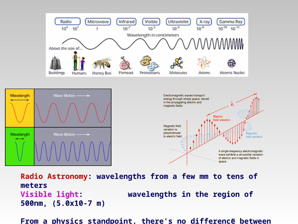
Radio Astronomy: wavelengths from a few mm to tens of metersVisible light: wavelengths in the region of 500nm, (5.0x10-7 m)

From a physics standpoint, there's no difference between visible light, and microwave/radio-wave “light”.

NRAO/AUI/NSF 5

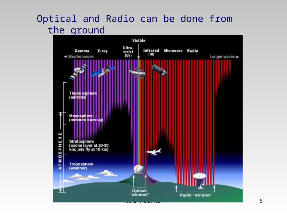
Optical and Radio can be done from the ground

θ ~λ/ D

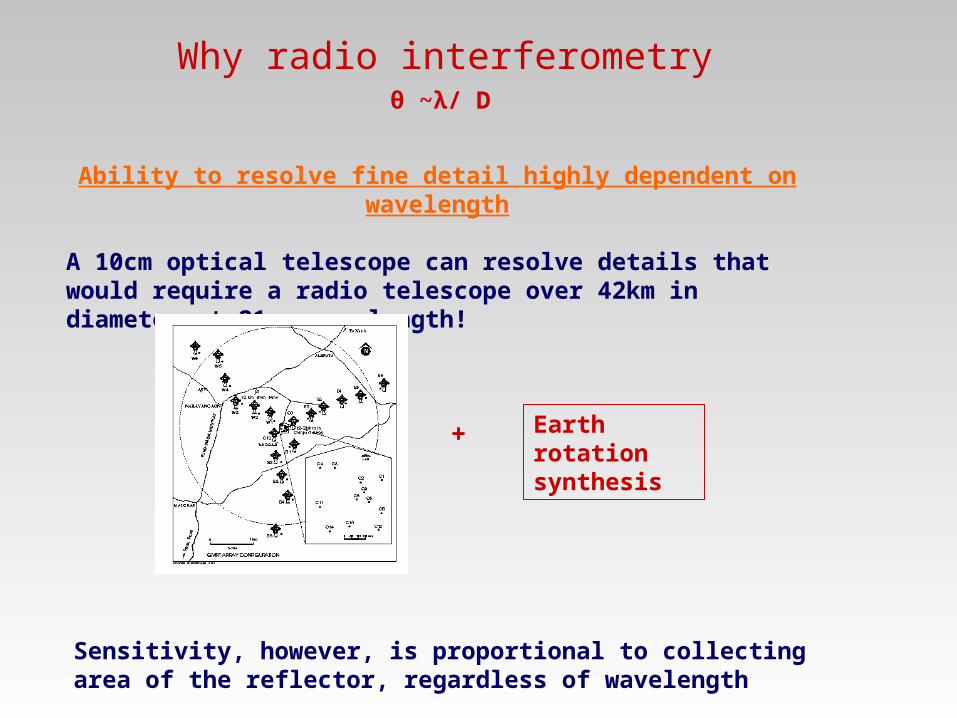
Ability to resolve fine detail highly dependent on wavelength

A 10cm optical telescope can resolve details that would require a radio telescope over 42km in diameter at 21cm wavelength!

Sensitivity, however, is proportional to collecting area of the reflector, regardless of wavelength

Why radio interferometry

Earth rotation synthesis

+

Angular resolutions at 20 cm (1.4 GHz)

D=100m θ ~ 9.4’

Effelsberg

EVLA D-array

D=1km θ ~ 44” D=28km θ ~ 1”

D=217 km θ ~ 150 mas

GMRT

D~10000 km θ ~ 5 mas

EVN

Connected elements

θ≈fraction of mas

HSTθ ~ 50 mas

(angular resolution of eMERLIN at

5 GHz)

Chandraθ~1”

(angular resolution of

the EVLA Array A and of the GMRT at 1.4 GHz)

GreenGMRT at 610 MHz

RedChandra

Overlay of the radio-optical & X-ray emission in a cluster of galaxies

OpticalDSS-2

Overlay of the radio-optical & X-ray emission in Centaurus A

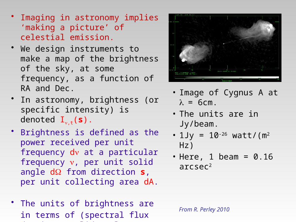
• Imaging in astronomy implies ‘making a picture’ of celestial emission.

• We design instruments to make a map of the brightness of the sky, at some frequency, as a function of RA and Dec.

• In astronomy, brightness (or specific intensity) is denoted In,t(s).

• Brightness is defined as the power received per unit frequency dn at a particular frequency n, per unit solid angle dW from direction s, per unit collecting area dA.

• The units of brightness are in terms of (spectral flux density)/(solid angle): e.g:

• watt/(m2 Hz Ster)

• Image of Cygnus A at l = 6cm.

• The units are in Jy/beam.• 1Jy = 10-26 watt/(m2 Hz)• Here, 1 beam = 0.16

arcsec2

From R. Perley 2010

Main Issues with interferometric observations

Phase corruption Calibration

u-v coverage Deconvolution & Imaging

Each pair of antennas in an interferometer is a baseline

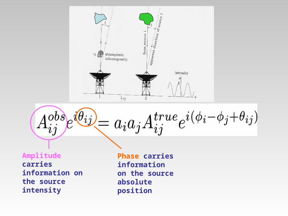
Amplitude carries information on the source intensity

Phase carries information on the source absolute position

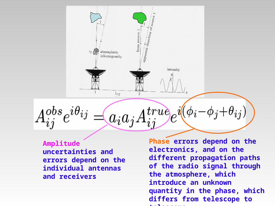
Amplitude uncertainties and errors depend on the individual antennas and receivers

Phase errors depend on the electronics, and on the different propagation paths of the radio signal through the atmosphere, which introduce an unknown quantity in the phase, which differs from telescope to telescope

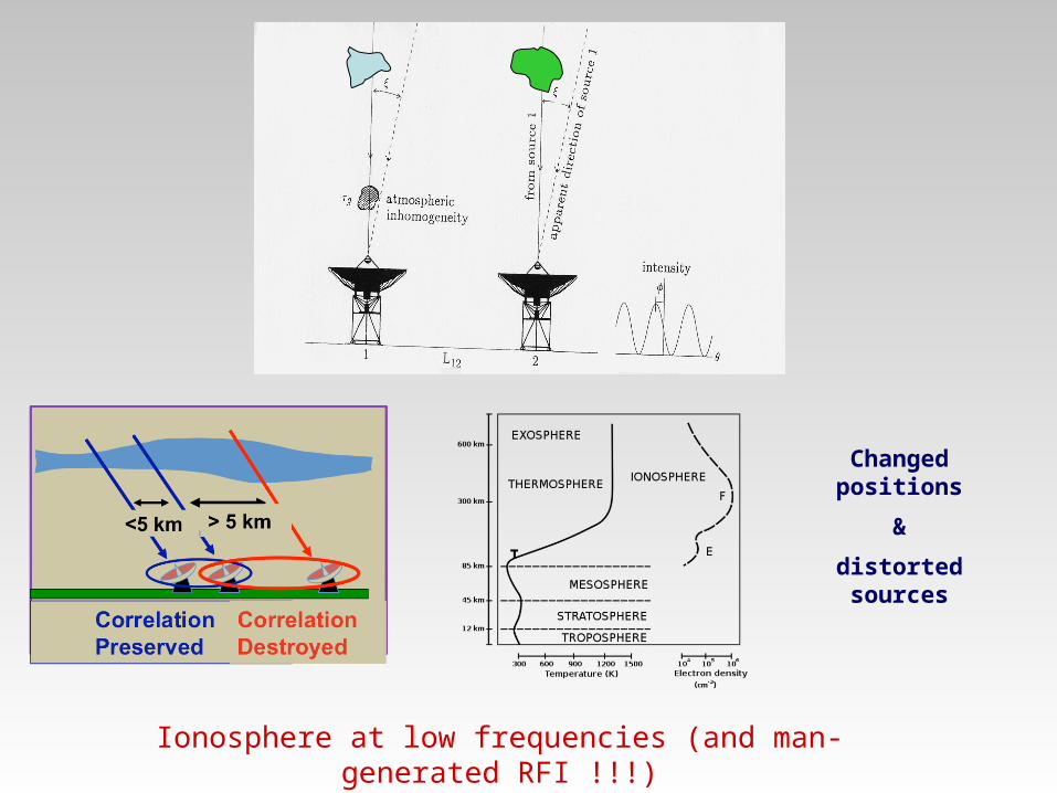
Changed positions &

distorted sources

Ionosphere at low frequencies (and man-generated RFI !!!)

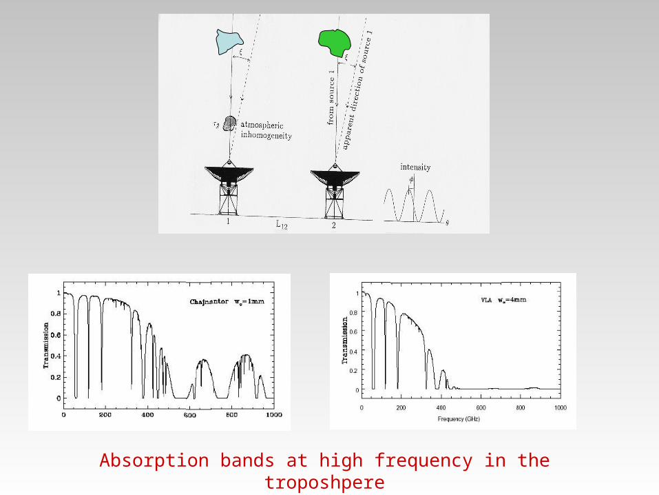
Absorption bands at high frequency in the troposhpere

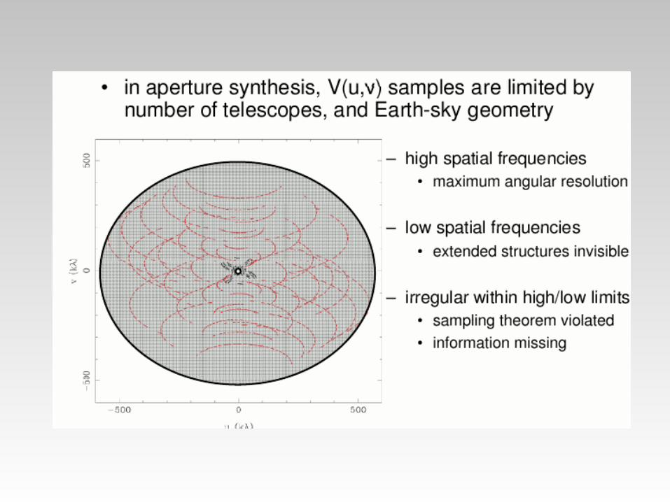
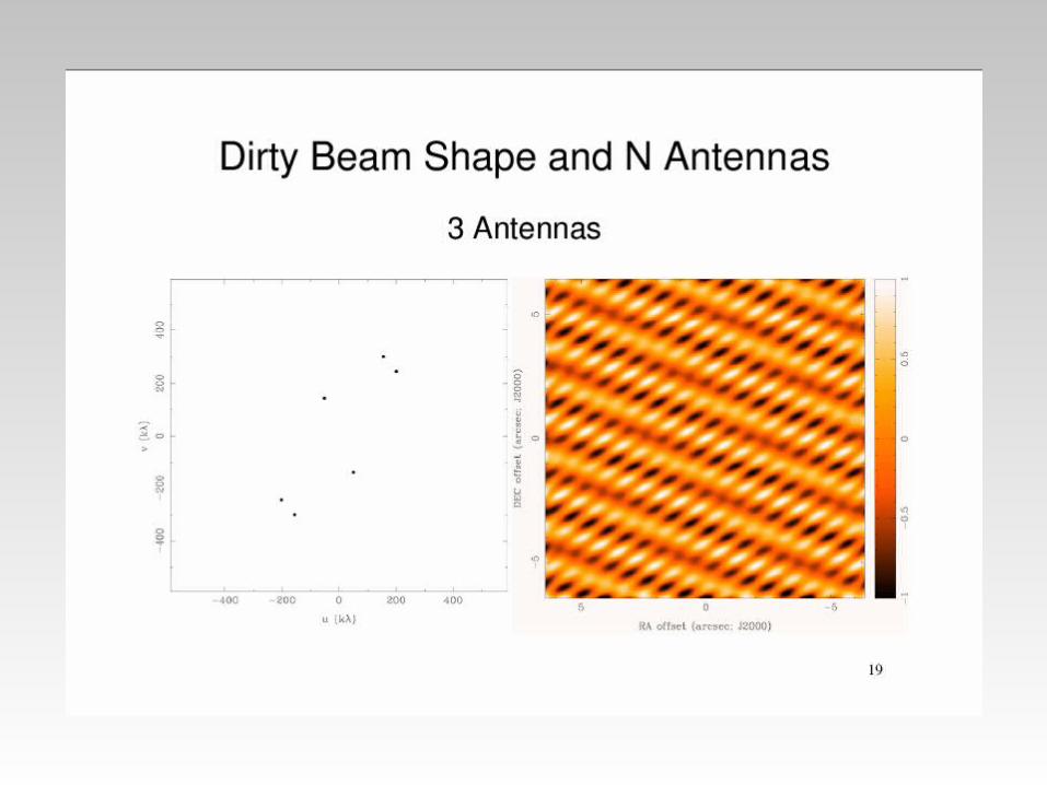
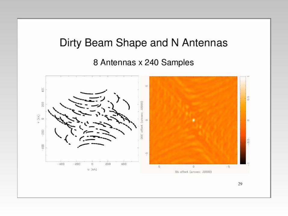
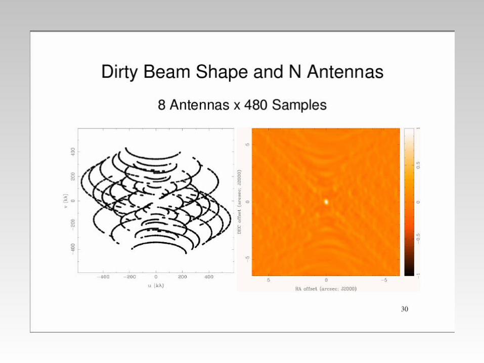
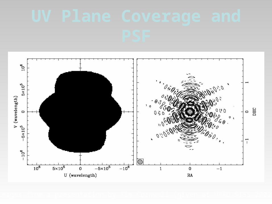
The u-v plane

A radio interferometer array can be considered as a partially filled aperture

- each pair of antennas gives a u-v point at a given time;

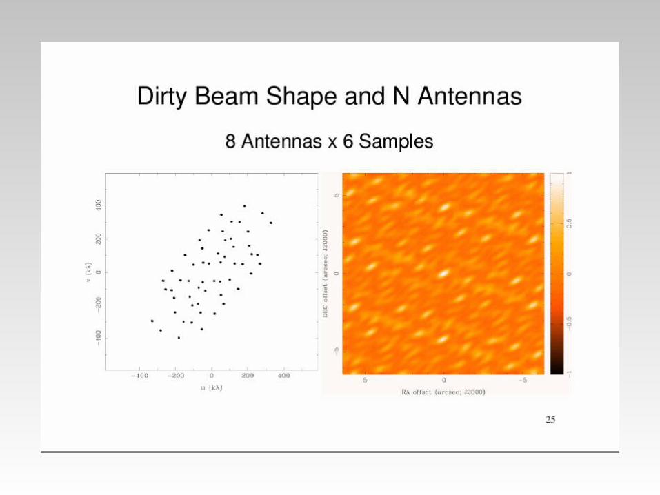
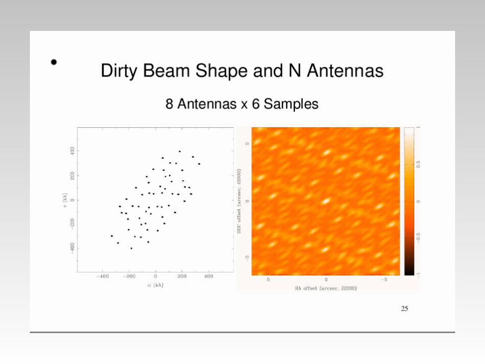
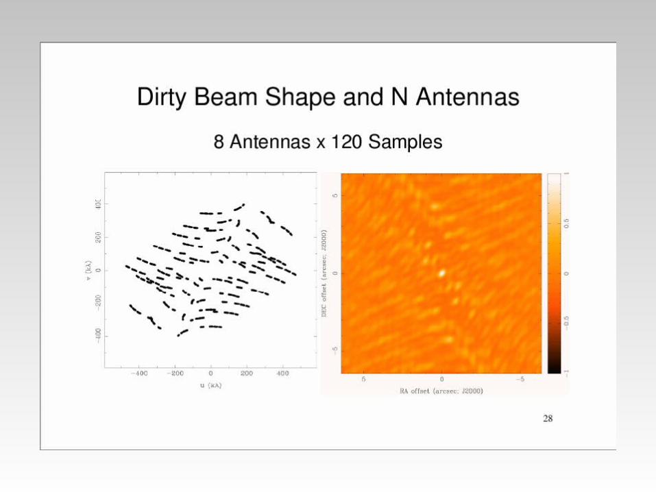
- the point source function (PSF, or beam) has a complicated structure, which depends on the array, source declination and u-v coverage;

- the u-v plane shows what part of the aperture is filled by a telescope, and this changes with time as the object rises and sets;

- a long exposure will have a better PSF/beam because there is better u-v plane coverage (closer to a filled aperture)

The u-v plane is a plane tangential to the source in the celestial sphere. Each point on that plane is the projection of a baseline at a given time.Each pair of radio telescopes produces a track in the u-v plane. The number of tracks is equivalent to N(N-1)/2, where N is the number of radio telescopes in the interferometer.

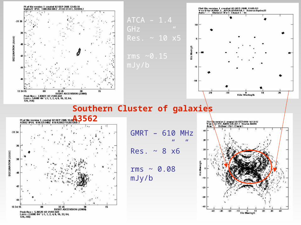
ATCA – 1.4 GHzRes. ~ 10”x5”

rms ~0.15 mJy/b

GMRT – 610 MHz

Res. ~ 8”x6”

rms ~ 0.08 mJy/b

Southern Cluster of galaxies A3562

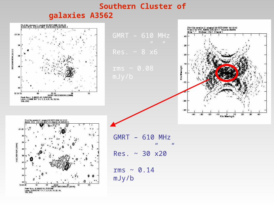
GMRT – 610 MHz

Res. ~ 8”x6”

rms ~ 0.08 mJy/b

Southern Cluster of galaxies A3562

GMRT – 610 MHz

Res. ~ 30”x20”

rms ~ 0.14 mJy/b

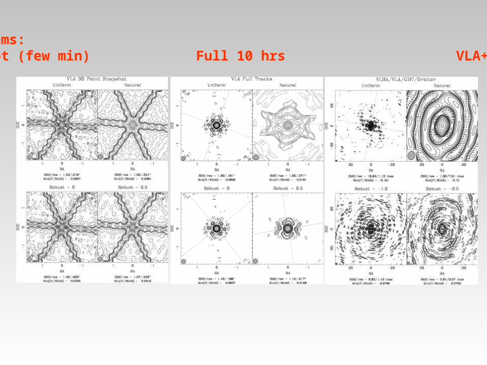
Dirty Beams:A snapshot (few min) Full 10 hrs VLA+VLBA+GBT

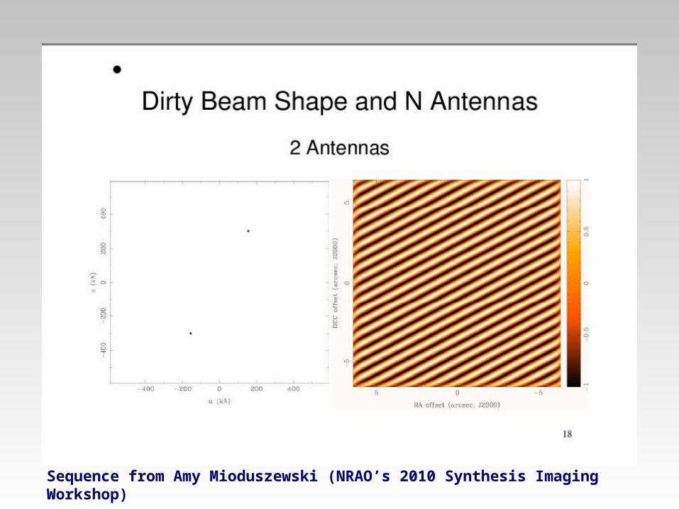
Sequence from Amy Mioduszewski (NRAO’s 2010 Synthesis Imaging Workshop)

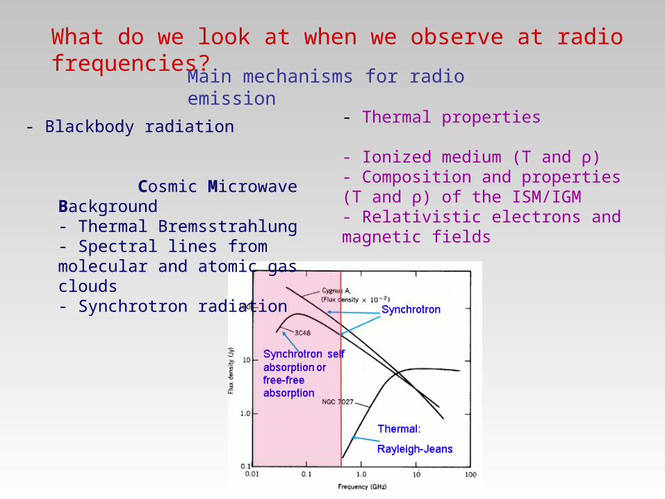
Main mechanisms for radio emission

- Blackbody radiation

Cosmic Microwave Background- Thermal Bremsstrahlung- Spectral lines from molecular and atomic gas clouds- Synchrotron radiation

What do we look at when we observe at radio frequencies?

- Thermal properties

- Ionized medium (T and ρ)- Composition and properties (T and ρ) of the ISM/IGM- Relativistic electrons and magnetic fields

• Emission from warm bodies– “Blackbody” radiation – Bodies with temperatures of

~ 3-30 K emit in the mm & submm bands

• Emission from accelerating charged particles– “Bremsstrahlung” or free-

free emission from ionized plasmas

Black body & Bremsstrahlung radiation

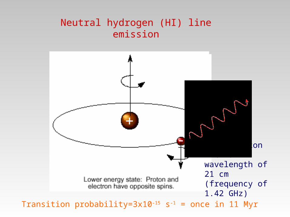
Emits photon with a wavelength of 21 cm (frequency of 1.42 GHz)

Transition probability=3x10-15 s-1 = once in 11 Myr

Neutral hydrogen (HI) line emission

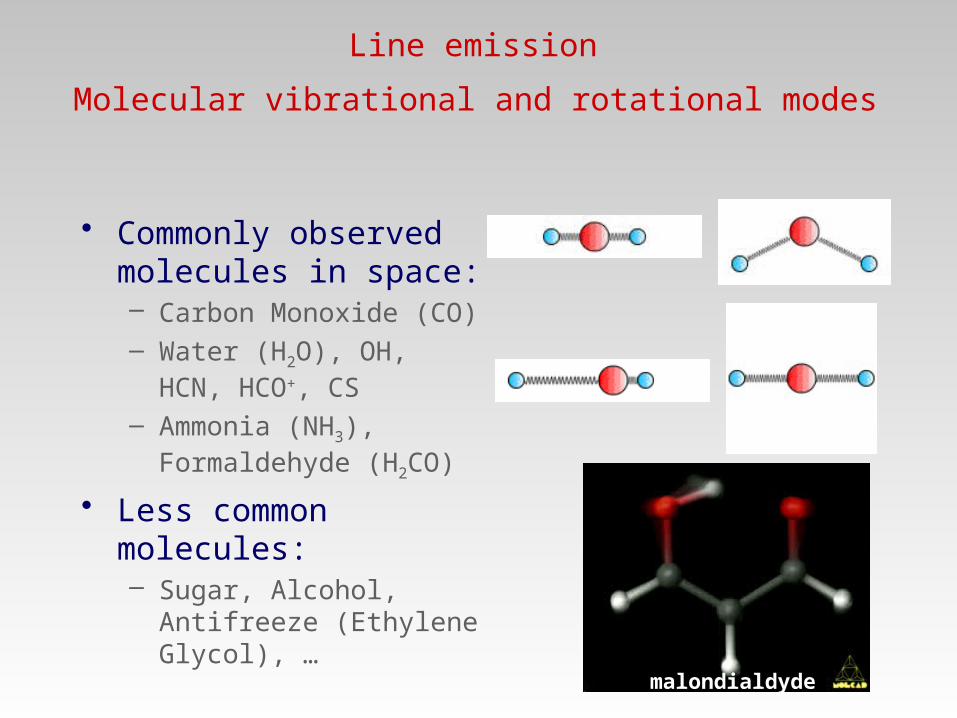
• Commonly observed molecules in space:– Carbon Monoxide (CO)– Water (H2O), OH, HCN,

HCO+, CS– Ammonia (NH3),

Formaldehyde (H2CO)• Less common molecules:

– Sugar, Alcohol, Antifreeze (Ethylene Glycol), …

malondialdyde

Line emission

Molecular vibrational and rotational modes

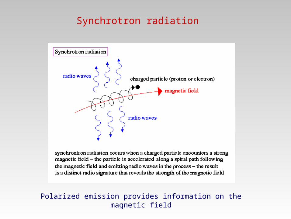
Synchrotron radiation

Polarized emission provides information on the magnetic field

Optically thin S α ν-α

Turnover

Optically thick/Self-absorbed

S α ν2.5

Spectrum of the synchrotron radiation

Aged part of the spectrum due to radiative losses

S α ν-(α+k)

Different parts of the synchrotron spectrum provide different information on the radio source and on the population of the radiating relativistic electrons

Steep spectrum dominated by the diffuse emission

Concave component dominated by the VLBI active nucleus

Example: an extragalactic radio source - 3C317

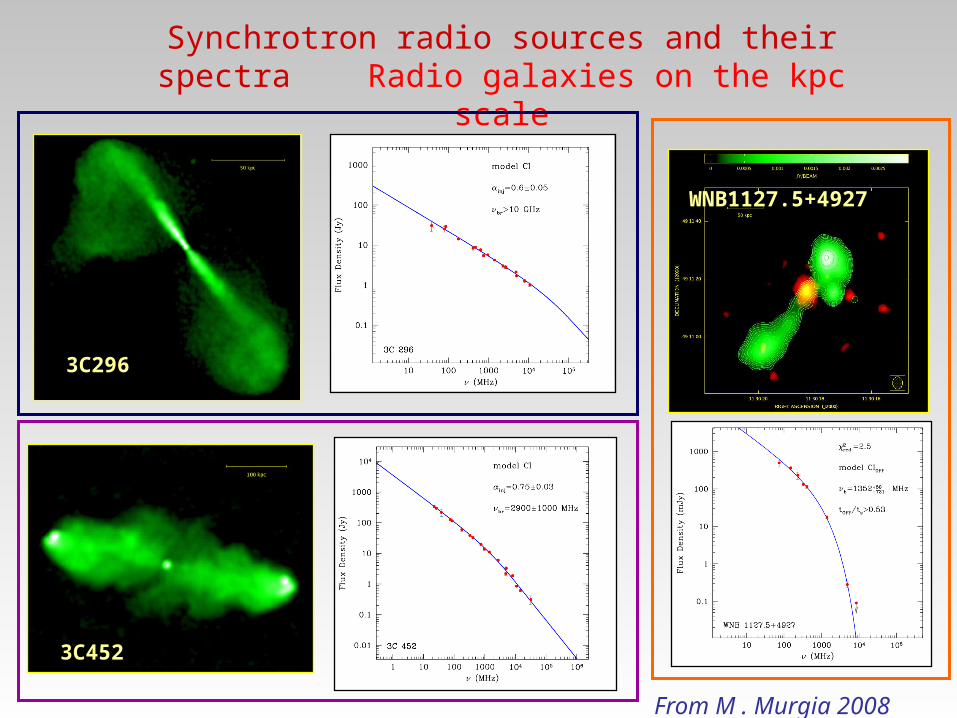
Synchrotron radio sources and their spectra Radio galaxies on the kpc scale

3C296

3C452

WNB1127.5+4927

From M . Murgia 2008

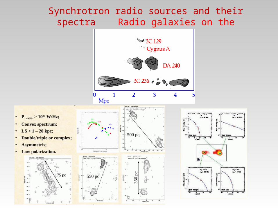
Synchrotron radio sources and their spectra Radio galaxies on the parsec scale

Synchrotron radio sources and their spectra Diffuse cluster sources

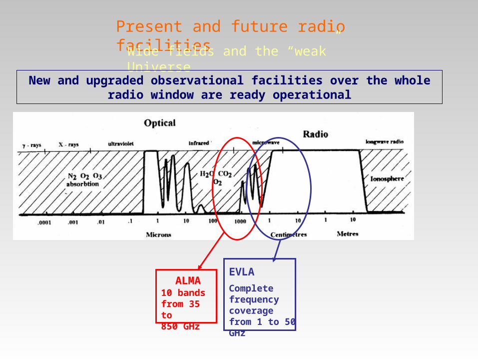
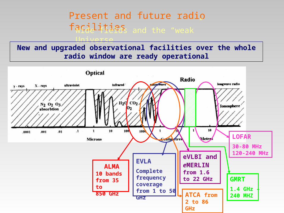
Present and future radio facilitiesWide fields and the “weak” Universe

ALMA 10 bands from 35 to 850 GHz

New and upgraded observational facilities over the whole radio window are ready operational

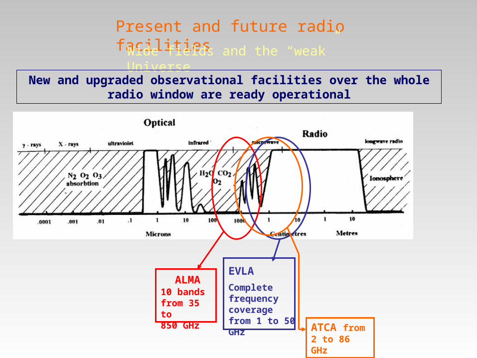
Present and future radio facilitiesWide fields and the “weak” Universe

ALMA 10 bands from 35 to 850 GHz

EVLAComplete frequency coverage from 1 to 50 GHz

New and upgraded observational facilities over the whole radio window are ready operational

Present and future radio facilitiesWide fields and the “weak” Universe

ALMA 10 bands from 35 to 850 GHz

EVLAComplete frequency coverage from 1 to 50 GHz

New and upgraded observational facilities over the whole radio window are ready operational

ATCA from 2 to 86 GHz

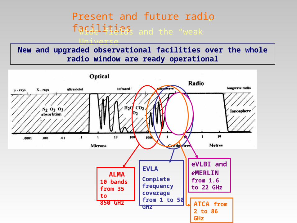
Present and future radio facilitiesWide fields and the “weak” Universe

ALMA 10 bands from 35 to 850 GHz

EVLAComplete frequency coverage from 1 to 50 GHz

eVLBI and eMERLIN from 1.6 to 22 GHz

New and upgraded observational facilities over the whole radio window are ready operational

ATCA from 2 to 86 GHz

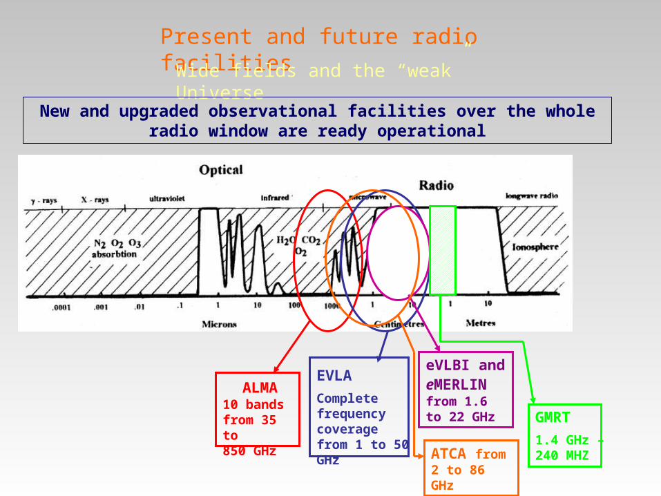
Present and future radio facilitiesWide fields and the “weak” Universe

ALMA 10 bands from 35 to 850 GHz

EVLAComplete frequency coverage from 1 to 50 GHz

eVLBI and eMERLIN from 1.6 to 22 GHz GMRT

1.4 GHz – 240 MHZ

New and upgraded observational facilities over the whole radio window are ready operational

ATCA from 2 to 86 GHz

Present and future radio facilitiesWide fields and the “weak” Universe

ALMA 10 bands from 35 to 850 GHz

EVLAComplete frequency coverage from 1 to 50 GHz

eVLBI and eMERLIN from 1.6 to 22 GHz

LOFAR30-80 MHz 120-240 MHz

GMRT 1.4 GHz – 240 MHZ

New and upgraded observational facilities over the whole radio window are ready operational

ATCA from 2 to 86 GHz

Enjoy the Fourth ERIS!

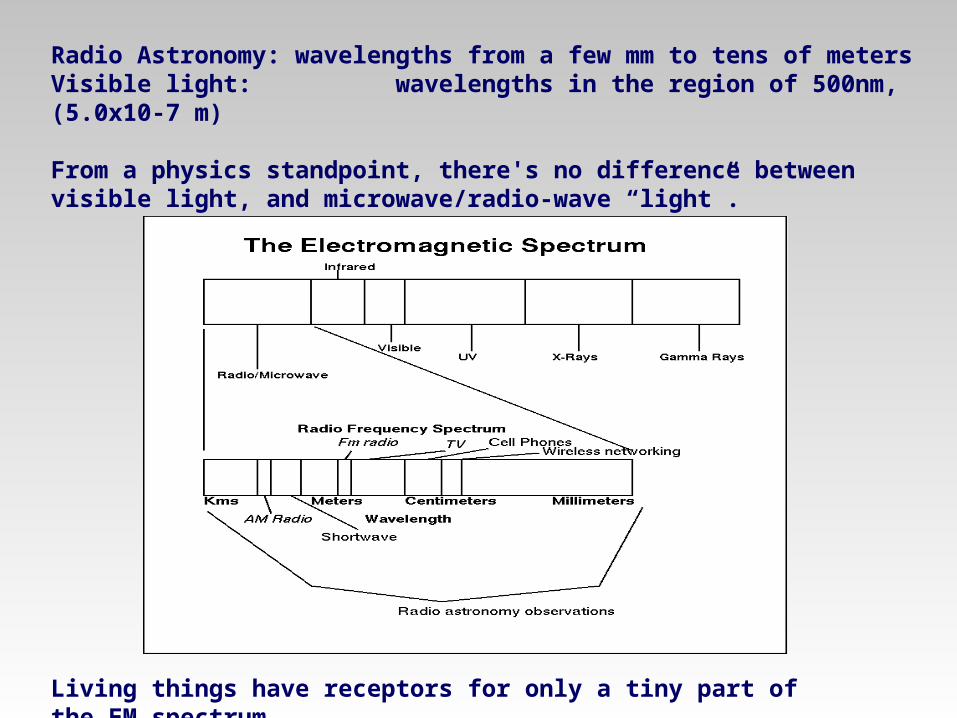
Radio Astronomy: wavelengths from a few mm to tens of metersVisible light: wavelengths in the region of 500nm, (5.0x10-7 m)

From a physics standpoint, there's no difference between visible light, and microwave/radio-wave “light”.

Living things have receptors for only a tiny part of the EM spectrum

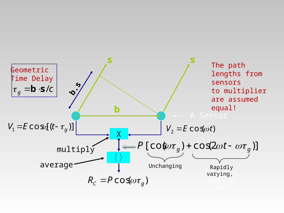
X

s s

A Sensorb

cg /sb

)(cos2 tEV ])(cos[1 gtEV

])2(cos)([cos gg tP multiply

average

b.s

The path lengths from sensors to multiplier are assumed equal!

Geometric Time Delay

Rapidly varying, with zero mean

Unchanging

)(cos gC PR

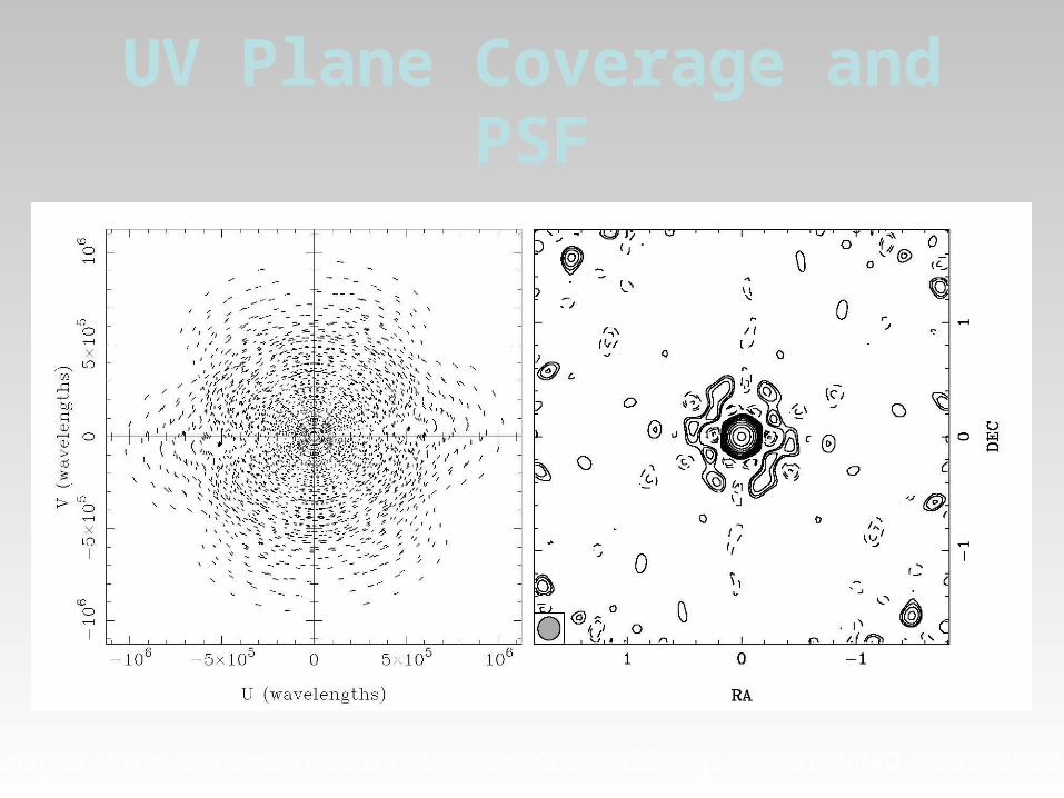
UV Plane Coverage and PSF

images from a presentation by Tim Cornwell (given at NRAO SISS 2002)

UV Plane Coverage and PSF

images from a presentation by Tim Cornwell (given at NRAO SISS 2002)

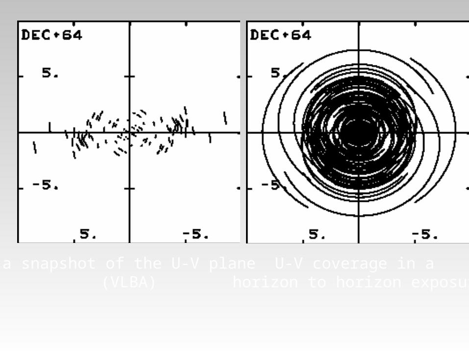
a snapshot of the U-V plane(VLBA)

U-V coverage in a horizon to horizon exposure

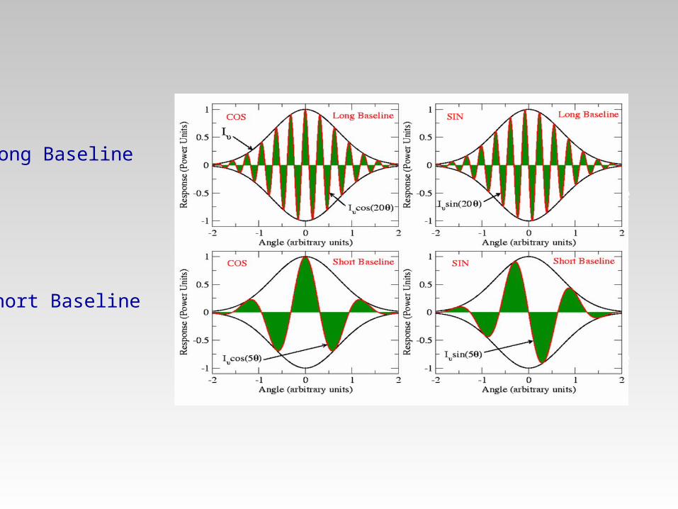
LongBaseline

ShortBaseline

Long Baseline

Short Baseline

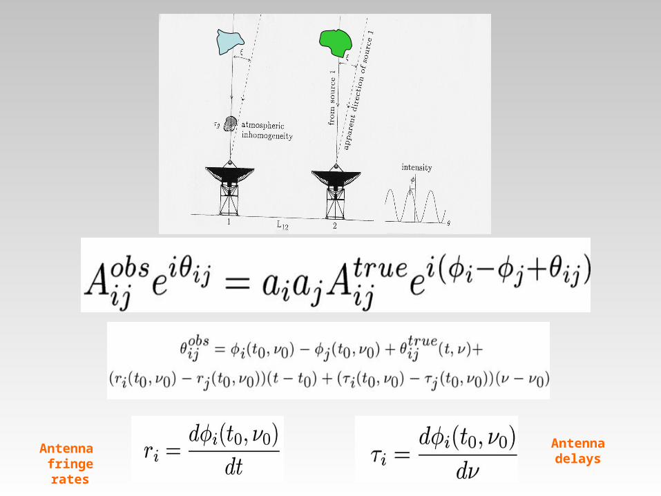
Antenna fringe rates

Antenna delays

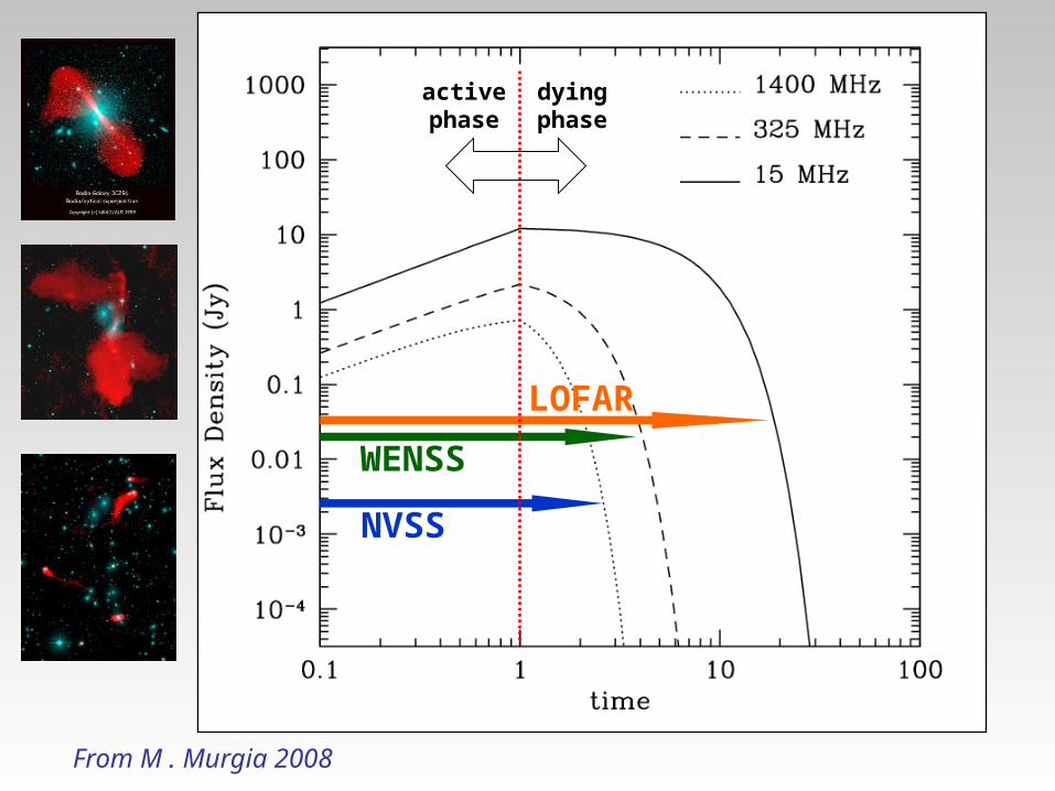
WENSS

NVSS

LOFAR

activephase

dyingphase

From M . Murgia 2008

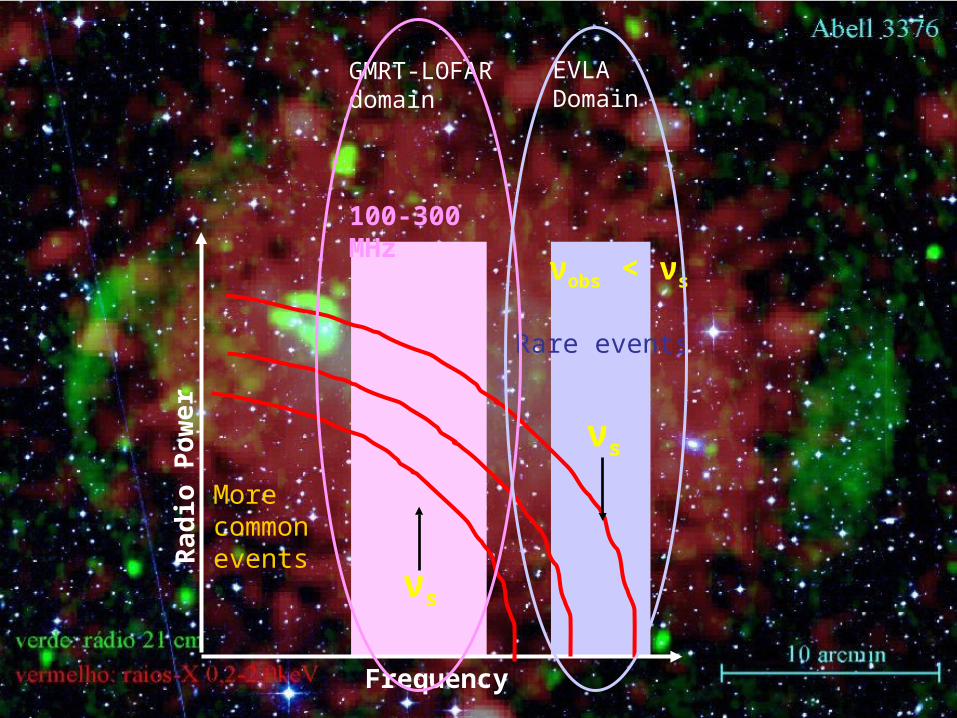
Rad

io P

ower

Frequency

νobs < νs

νs

νs

More common events

Rare events

100-300 MHz

GMRT-LOFAR domain

EVLA Domain