interferometric synthetic aperture radar - an … · an introduction for users of insar data ... in...

INTERFEROMETRIC SYNTHETIC

APERTURE RADAR

An Introduction for Users of InSAR

Data

Page | 2

Table of Contents

An Introduction for Users of InSAR Data ...................................................................................... 5

1. Background .......................................................................................................................... 5

2. Basics of Synthetic Aperture Radar (SAR) .......................................................................... 5

2.1 Satellites ................................................................................................................... 5

2.2 SAR Sensors ............................................................................................................. 7

2.3 SAR Image Acquisition ............................................................................................ 7

2.4 Radar Frequencies and Viewing Geometry .............................................................. 8

2.5 Signal Properties ....................................................................................................... 9

2.6 Satellite Orbits and Geometrical Distortions .......................................................... 11

2.7 Resolution ............................................................................................................... 13

3. Basics of InSAR ................................................................................................................. 14

3.1 Interferometry ......................................................................................................... 14

3.2 Interferograms ........................................................................................................ 15

3.3 Contributors to Signal Phase .................................................................................. 16

3.4 Coherence ............................................................................................................... 17

4. Differential InSAR (DInSAR) ............................................................................................ 18

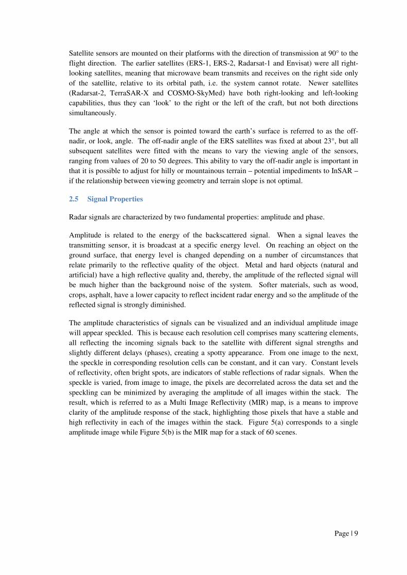
5 Interferogram Stacking ....................................................................................................... 19

6. Persistent Scatterer Techniques .......................................................................................... 20

6.1 General Concept ..................................................................................................... 20

6.2 Permanent Scatterers .............................................................................................. 20

6.3 Calculating Displacement ....................................................................................... 21

6.4 Precision ................................................................................................................. 22

6.5 Validation of PS Data ............................................................................................. 23

6.6 Data Output and Presentation ................................................................................. 24

7. SqueeSAR .......................................................................................................................... 25

8. Artificial Reflectors (AR) ................................................................................................... 27

9. Strengths and Weaknesses of PS Analyses ........................................................................ 28

10. Synergistic Use of PS and GPS ........................................................................................ 29

APPENDIX.................................................................................................................................... 31

GLOSSARY ................................................................................................................................... 32

PROCESS MAP ............................................................................................................................. 34

Page | 3

Table of Figures

Figure 1 Satellite Radar Systems available now and into the future. ........................................... 6

Figure 2: Illustration of the relationship between the orbit path of the satellite and true North –

South. It varies from satellite to satellite but is generally around 10° (see Section 2.6 for

definition of ascending and descending orbits). ........................................................................... 6

Figure 3: Schematic showing how a satellite acquires a strip map of the earth’s surface. ........... 8

Figure 4: Schematic showing the orientation of signal launch toward the earth’s surface........... 8

Figure 5(a-b): Images showing the effect of multi image reflectivity (MIR). ............................ 10

Figure 6: Motion measured by the sensor for different directions of terrain-motion. Red arrows

represent the vector of terrain motion while blue arrows represent the LOS motion measured by

the radar system. ......................................................................................................................... 11

Figure 7: Illustration of the method for obtaining actual motion by combining ascending and

descending orbit information. In the case of vertical ground displacements (left image) the

motion components on the ascending and descending directions are both negative (moving

away from the sensor) while in the case of a horizontal (E-W) motion (right image) one vector

is positive (moving toward the sensor) while the other is negative. ........................................... 11

Figure 8: Schematic illustration showing how features on the landscape are projected on to the

line of sight of the satellite radar beam. ...................................................................................... 12

Figure 9: An amplitude image of Mt. Vesuvius, in SAR coordinates. The North direction is to

the left of the image (the satellite flies from left to right in a descending orbit). The coast line

along the Tyrrhenian Sea is clearly visible (water appears as black). Urban areas can be

identified as bright spots on the image created by the strong amplitude responses from

reflections off buildings. The eastern slopes of the volcano (at the top of the image) are

‘compressed’ compared to those on the western slopes (foreshortening). ................................. 12

Figure 10: Schematic illustration showing how mountainous terrain can create noise through

layover and shadow effects......................................................................................................... 13

Figure 11: A schematic showing the relationship between ground displacement and signal

phase shift. The numerical value of the wavelength is that of ERS. .......................................... 15

Figure 12: An interferogram generated from two radar images one of which was acquired

before the L’Aquila earthquake (February 2009) and the other shortly after the event (April

2009). The fringes indicate coherence whereby displacement can be calculated in the

corresponding areas. The areas with a spotty appearance are areas where decorrelation noise

has occurred. Phase values range from –π to +π. ....................................................................... 16

Figure 13. The visual display of results of a PSInSAR™ analysis of Lake Presenzano and its

surrounding area. ........................................................................................................................ 21

Page | 4

Figure 14: A typical time series showing linear and non-linear patterns of movement. ............ 22

Figure 15: Typical values of precision (1 sigma) for a point less than 1km from the reference

point (P0), considering a multi-year dataset of radar images. ..................................................... 23

Figure 16: Comparison of PSInSAR™ with GPS data. The x, y and z components of GPS

measurements have been resolved to the equivalent LOS of the satellite data. ......................... 23

Figure 17: Optical leveling. The blue line is an optical benchmark correction curve; the red dots

represent InSAR readings at the same location. ......................................................................... 24

Figure 18: Thermal Dilation. Buildings move in response to changes in temperature and

software is available to model such movement. The black line represents the results of a

thermal dilation model while the red triangles correspond to InSAR readings on the same

building, measured over the same time period. .......................................................................... 24

Figure 19(a-c): These images are screen-grabs from a GIS showing how distant and close-up

views of deformation phenomena can be observed using GIS platforms. .................................. 25

Figure 20(a-d): Artificial reflectors. ........................................................................................... 28

Figure 21: The Right Bank Landslide, Lake Sarez, Tajikistan showing the results of analyses of

movement using both GPS and PSInSAR™ technologies. ........................................................ 30

Table of Tables

Table 1: Nominal Resolution Cell Sizes of all Commercial Radar Satellites. Numbers in

brackets, for COSMO-SkyMed data, refer to the use of 2 satellites of the constellation,

operating in tandem. ................................................................................................................... 14

Table 2: Summary of strengths and weaknesses of InSAR ........................................................ 28

Table 3: Comparison of PS and GPS technologies .................................................................... 29

Page | 5

INTERFEROMETRIC SYNTHETIC APERTURE RADAR

An Introduction for Users of InSAR Data

1. Background

This document is a general overview of the concepts related to the measurement of surface

deformation phenomena using Synthetic Aperture Radar Interferometry (InSAR). The text has

been written in layman terms, avoiding radar specialist jargon. Should the reader be interested

in a more detailed explanation, he/she can refer to the suggested supplementary reading,

appended to this document.

The two main fields of application of InSAR data are: a) reconstruction of digital elevation

models of large areas; b) detection and monitoring of surface deformation phenomena and, in

general c) measurement of displacement rates of objects on the ground. In this document, the

focus will be on the latter topic.

The first theoretical study on this subject dates back to the 1980s (Gabriel et al., 1989) when the

first proof of concept using SEASAT data was published by the Jet Propulsion Laboratory’s

radar group. With the launch of the European Space Agency’s (ESA) ERS-1 satellite, in July

1991, and ERS-2, in April 1995, an ever-growing set of interferometric data became available

to many research groups. While more and more InSAR results were generated, the presence of

atmospheric artifacts became more and more evident and dampened, somewhat, the

enthusiasm. Research efforts were then devoted to different strategies for the combination of

several interferograms or the fusion of InSAR data with prior information, in order to reduce

the impact of the atmospheric disturbances.

Among several research groups pursuing this challenge was the Department of Electrical

Engineering of the Politecnico di Milano, in Italy. By 1999, the Institution had developed the

Permanent Scatterer Technique along with its proprietary PSInSAR™ algorithm. In March

2000, the Politecnico di Milano and the three inventors of the technology founded TRE, to

create a team specialized in InSAR data processing. Since that time, other organizations have

developed similar technologies, but TRE has still the largest team of engineers specifically

working on SAR interferometry.

2. Basics of Synthetic Aperture Radar (SAR)

2.1 Satellites

The family of satellites that carry, or will be carrying, SAR sensors for commercial applications

is illustrated in Figure 1. Other SAR-bearing satellites exist but are used exclusively for

military applications.

Page | 6

Figure 1 Satellite Radar Systems available now and into the future.

All satellites equipped with SAR sensors orbit the earth on a near-polar orbit at an altitude

ranging from 500 to 800 km above the earth’s surface, depending on the satellite platform

hosting the SAR sensor.

The angle between true north-south and the satellite orbit varies slightly, depending on the

satellite but, in general lies in the range of 10 degrees, as shown in Figure 2.

Ascending Orbit

Descending Orbit

Figure 2: Illustration of the relationship between the orbit path of the satellite and true North –

South. It varies from satellite to satellite but is generally around 10° (see Section 2.6 for definition of

ascending and descending orbits).

Page | 7

Data from different satellite sources can generally be purchased or ordered without limitation,

with the exception of data from the Japanese Space Agency (JAXA). Although ALOS-

PALSAR data can be purchased, JAXA selected the acquisition modes of the satellite for the

duration of its operating life (past and future), at the beginning of the mission, so the user

cannot select the radar acquisition mode most suitable for the application at hand.

Another important point to be considered is that the Italian COSMO-SkyMed constellation is a

joint military/civilian mission. Whenever a conflict arises between acquisition requests,

commercial projects have lower priority.

2.2 SAR Sensors

Because the illuminating source of radar is microwave energy, radar signals are unaffected by

darkness or clouds, in terms of visibility of the land surface. As will be discussed later, clouds

impact the accuracy of InSAR but do not obstruct the passage of the signal through the

medium. Therefore, SAR can function 24 hours per day, 365 days per year.

The sensors emit signals with a specific central frequency. In addition, radar systems are

associated with specific bands of the electromagnetic spectrum. Those commonly used in

InSAR applications are L-band (1-2 GHz, ~24 cm wavelength), C-band (5-6 GHz, ~6 cm

wavelength) and X-band (8-12 GHz, ~3 cm wavelength).

In 1992, with the launch of ERS-1, the first SAR satellite for commercial applications, the on-

board sensor offered but one acquisition mode, a single look angle, a single resolution cell size,

and a single signal wavelength. The only options available related to viewing geometry, i.e.

ascending or descending satellite tracks. Today, as Figure 1 indicates, the options have

proliferated with the increase in numbers of satellites, offering the end-user a wide choice of

look angle, repeat orbit cycle, resolution cell size, and signal wavelength. It is now possible to

design a monitoring program much better suited to an end-user’s needs than was possible 10

years ago.

2.3 SAR Image Acquisition

As the satellite circumnavigates the earth, it launches millions of radar signals toward the earth

along the radar beam’s line of sight (LOS), on a continuous basis. Following impact with the

earth’s surface, some of the signals are reflected away from the satellite, some are absorbed in

vegetation or other non-reflective materials and some reflect back to the satellite. Using the

signals reflected off the earth’s surface, also referred to as backscattered signals, processors on

board the satellite integrate the returning signals to form a strip map. Usually, the on board

memory capacity is limited so the satellite has to transmit the data to strategically located

ground stations. These stations then compile images which can be used for data analysis.

Figure 3 is a schematic showing the process of image acquisition by a satellite.

Figure 3: Schematic showing how a satellite acquires a strip map of the earth

2.4 Radar Frequencies and

Radar signals are transmitted in pulses

important frequencies that define its operations.

(PRF) is the rate at which those pulses are transmitted

in azimuth direction (i.e. the direction parallel to the satellite velocity)

(f0) defines the operating wavelength of the system and

penetration features, as well as the sensitivity of the system in interferometric applications

Finally, radar pulses backscattere

another frequency (fs) defining the

cell size, in the range direction

Figure 4: Schematic showing the orientation of signal launch toward the earth’s surface

: Schematic showing how a satellite acquires a strip map of the earth

Radar Frequencies and Viewing Geometry

transmitted in pulses (Figure 4). In any SAR system, there are three

important frequencies that define its operations. The so-called Pulse Repetition F

is the rate at which those pulses are transmitted and defines the resolution of the system

in azimuth direction (i.e. the direction parallel to the satellite velocity), the

operating wavelength of the system and characterizes its propagation and

, as well as the sensitivity of the system in interferometric applications

adar pulses backscattered by the Earth surface are sampled by the radar system at

defining the nominal pixel size, sometimes referred to as the resolution

cell size, in the range direction, related to the sensor-to-target distance.

: Schematic showing the orientation of signal launch toward the earth’s surface

Page | 8

: Schematic showing how a satellite acquires a strip map of the earth’s surface.

In any SAR system, there are three

called Pulse Repetition Frequency

and defines the resolution of the system

the central frequency

izes its propagation and

, as well as the sensitivity of the system in interferometric applications.

sampled by the radar system at

pixel size, sometimes referred to as the resolution

: Schematic showing the orientation of signal launch toward the earth’s surface.

Page | 9

Satellite sensors are mounted on their platforms with the direction of transmission at 90° to the

flight direction. The earlier satellites (ERS-1, ERS-2, Radarsat-1 and Envisat) were all right-

looking satellites, meaning that microwave beam transmits and receives on the right side only

of the satellite, relative to its orbital path, i.e. the system cannot rotate. Newer satellites

(Radarsat-2, TerraSAR-X and COSMO-SkyMed) have both right-looking and left-looking

capabilities, thus they can ‘look’ to the right or the left of the craft, but not both directions

simultaneously.

The angle at which the sensor is pointed toward the earth’s surface is referred to as the off-

nadir, or look, angle. The off-nadir angle of the ERS satellites was fixed at about 23°, but all

subsequent satellites were fitted with the means to vary the viewing angle of the sensors,

ranging from values of 20 to 50 degrees. This ability to vary the off-nadir angle is important in

that it is possible to adjust for hilly or mountainous terrain – potential impediments to InSAR –

if the relationship between viewing geometry and terrain slope is not optimal.

2.5 Signal Properties

Radar signals are characterized by two fundamental properties: amplitude and phase.

Amplitude is related to the energy of the backscattered signal. When a signal leaves the

transmitting sensor, it is broadcast at a specific energy level. On reaching an object on the

ground surface, that energy level is changed depending on a number of circumstances that

relate primarily to the reflective quality of the object. Metal and hard objects (natural and

artificial) have a high reflective quality and, thereby, the amplitude of the reflected signal will

be much higher than the background noise of the system. Softer materials, such as wood,

crops, asphalt, have a lower capacity to reflect incident radar energy and so the amplitude of the

reflected signal is strongly diminished.

The amplitude characteristics of signals can be visualized and an individual amplitude image

will appear speckled. This is because each resolution cell comprises many scattering elements,

all reflecting the incoming signals back to the satellite with different signal strengths and

slightly different delays (phases), creating a spotty appearance. From one image to the next,

the speckle in corresponding resolution cells can be constant, and it can vary. Constant levels

of reflectivity, often bright spots, are indicators of stable reflections of radar signals. When the

speckle is varied, from image to image, the pixels are decorrelated across the data set and the

speckling can be minimized by averaging the amplitude of all images within the stack. The

result, which is referred to as a Multi Image Reflectivity (MIR) map, is a means to improve

clarity of the amplitude response of the stack, highlighting those pixels that have a stable and

high reflectivity in each of the images within the stack. Figure 5(a) corresponds to a single

amplitude image while Figure 5(b) is the MIR map for a stack of 60 scenes.

Page | 10

Figure 5(a) An ERS-2 SAR amplitude image of Linate Airport in Milan (Italy): the speckle effect on

the fields surrounding the airport is clearly visible.

Figure 5(b): An MIR map of the same area at Linate Airport: the speckle effect on the fields

surrounding the airport has disappeared.

Figure 5(a-b): Images showing the effect of multi image reflectivity (MIR).

Apart from amplitude values, radar systems record phase values, the key element in any

interferometric measurement, since it is related to the sensor-to-target distance. As has already

been mentioned, radar signals are characterized by a certain frequency of operation and, for

interferometric applications, they can be thought of as sinusoidal waves: one complete cycle

(from –π to +π) corresponding to the wavelength. It is this specific property of the radar signal,

and the system’s ability to record both amplitude and phase information for each image pixel,

that are used in estimating displacement.

A signal’s phase can be affected by changes in the atmosphere as it travels from the satellite to

the earth and then back again. In the atmosphere, there are always layers of moisture (cloud,

fog, rain etc.) through which a signal must pass. In arid areas, these layers are few compared to

tropical and temperate areas. As a signal encounters a moisture-bearing layer in the atmosphere,

the propagating speed of the signal changes. As a result, errors are introduced into the phase

values recorded by the receiving sensor, on the satellite. Since wavelength and signal phase

have a simple and direct correlation, any change in wavelength corresponds to a change in the

phase of a signal. As will be explained later in Section 3, this is an important issue in

measuring ground movement because there is also a direct relationship between ground

displacement and signal phase.

Page | 11

2.6 Satellite Orbits and Geometrical Distortions

The circumpolar orbits of all satellites mean that, for part of their trajectory, they are travelling

from the North toward the South. This direction is referred to as Descending. Conversely,

when the satellite is traveling from the South toward the North, it is said to be in an Ascending

orbit. By acquiring imagery during both ascending and descending orbits, it is possible to view

a point on the earth’s surface from two different perspectives, from the East or from the West.

This is an important element of measuring vertical and horizontal motion.

What is actually measured in interferometric applications is the projection of a target’s motion

onto the LOS. If the motion direction is close to the angle of the LOS then the measured and

actual motions will be similar. However, the LOS motion can often differ noticeably from the

real value of motion, especially in cases where the ground motion is not vertical (Figure 6).

Figure 6: Motion measured by the sensor for different directions of terrain-motion. Red arrows

represent the vector of terrain motion while blue arrows represent the LOS motion measured by the

radar system.

Measuring true vertical and horizontal components of motion is difficult with a single geometry

acquisition, unless a priori information is available on the true vector of movement (not a

common situation!). However, by using ascending and descending data together, it is possible

to combine the measured motion information to obtain an accurate estimate of the actual

vertical motion and of the East-West component of the motion (Figure 7).

Figure 7: Illustration of the method for obtaining actual motion by combining ascending and

descending orbit information. In the case of vertical ground displacements (left image) the motion

components on the ascending and descending directions are both negative (moving away from the

sensor) while in the case of a horizontal (E-W) motion (right image) one vector is positive (moving

toward the sensor) while the other is negative.

Page | 12

Figure 8 illustrates how features on an undulating landscape will be viewed by the satellite. In

pixels (resolution cells) 1 and 2, the equilateral triangles on the landscape appear slightly

distorted in the LOS (range, sometimes referred to as slant-range). As the signal reaches pixel

3, there is a marked change in ground slope and many more triangles appear in the pixel, even

though they are all of the same size. The effect is to compress these triangles in the LOS,

referred to as foreshortening. When the radar progresses to pixels 4 and 5, at which point the

ground slope and LOS are parallel, the triangles now appear stretched at their base. This

distortion in the appearance of land use can be seen in Figure 9, which is an amplitude image of

Mount Vesuvius, in Italy, viewed in SAR coordinates (range and azimuth, corresponding to the

vertical and horizontal axis, respectively).

Figure 8: Schematic illustration showing how features on the landscape are projected on to the line of

sight of the satellite radar beam.

Figure 9: An amplitude image of Mt. Vesuvius, in SAR coordinates. The North direction is to the left

of the image (the satellite flies from left to right in a descending orbit). The coast line along the

Tyrrhenian Sea is clearly visible (water appears as black). Urban areas can be identified as bright

spots on the image created by the strong amplitude responses from reflections off buildings. The

eastern slopes of the volcano (at the top of the image) are ‘compressed’ compared to those on the

western slopes (foreshortening).

Ground rangeGround range

Slant-range

Slant-range

TopographyTopography

Sla

nt-r

ange

Sla

nt-r

ange

reso

lution

reso

luti

on

1 2 3 4 5

Off-Nadir

Azimuth

Ran

ge

Page | 13

In hilly or mountainous terrain, it sometimes occurs that the projection of steep slopes on to the

LOS is reversed. Figure 10 illustrates how this phenomenon manifests itself in radar imagery.

In pixel 1, the radar “sees” the object A normally. However, when the radar reaches pixels 2, 3

and 4, the objects E, F, and G are present in the same pixels as objects B, C, and D, the latter

being masked by the former. This phenomenon is referred to as “layover” and generates noise.

In an amplitude image, it appears as a bright white layer and, in Figure 9 , it can be observed

around the caldera of Mount Vesuvius. As the radar progresses from pixels 4 to 7, the slope of

the ground is greater than that of the LOS and, so, the area in question cannot be “seen” by the

sensor and, in an amplitude image, appears as a black area, as can also be seen in Figure 9.

This effect is referred to as “shadow”.

Figure 10: Schematic illustration showing how mountainous terrain can create noise through layover

and shadow effects.

2.7 Resolution

To most end-users of interferometric data the terms resolution and pixel are usually

synonymous. They are different, however, although similar in numerical value. The

explanation of the difference is rooted in signal processing theory and is beyond the scope of

this User Manual. Accordingly, the resolution in the range and azimuth directions are usually

referred to in nominal value terms and, for the various satellites that carry SAR sensors, these

values are shown in Table 1.

Page | 14

Satellite Band Acquisition Mode Nominal Pixel

Dimension:

ground range x

azimuth (m)

Repeat Cycle

(day)

ERS-1 & ERS-2 C Standard Beam 20x4 35

Envisat C Standard Beam 20x4 35

Radarsat-1 C Standard Beam 20x5 24

Radarsat-1 C Fine Beam 10x5 24

Radarsat-2 C Standard Beam 20x5 24

Radarsat-2 C Fine Beam 10x5 24

Radarsat-2 C Ultra Fine Beam 3x3 24

TerraSAR-X X Standard 3x3 11

TerraSAR-X X Spotlight 1.5x1.5 11

Cosmo SkyMed X Standard 3x3 16 (8)

Cosmo SkyMed X Spotlight 1.5x1.5 16 (8)

ALOS PALSAR L Fine Beam 10x5 46

Table 1: Nominal Resolution Cell Sizes of all Commercial Radar Satellites. Numbers in brackets, for

COSMO-SkyMed data, refer to the use of 2 satellites of the constellation, operating in tandem.

The values in Table 1 relate to a land surface that is flat and horizontal. In reality, much of the

earth’s landscape contains land that is irregular in surface profile (hills, valleys etc.) and these

features immediately impact the actual dimensions of the resolution cell.

3. Basics of InSAR

3.1 Interferometry

Interferometric Synthetic Aperture Radar (InSAR), also referred to as SAR Interferometry, is

the measurement of signal phase change, or interference, over time. When a point on the

ground moves, the distance between the sensor and the point on the ground also changes and so

the phase value recorded by a SAR sensor flying along a fixed orbit will be affected, too.

Figure 11 shows the relationship between that ground movement and the corresponding shift in

signal phase between two SAR signals acquired over the same area.

Figure 11: A schematic showing the relationship between ground displacement and signal phase

shift. The numerical value of the wavelength is that of

The change in signal phase (

Where λ is the wavelength

atmospheric conditions at the time of the two

displacement of a radar target along the satellite line of sight creates

signal that can be detected by comparing the phase values of two SAR images acquired at

different times.

Apart from decorrelation effects, to be discussed in the next sections, SAR i

only be applied in the following circumstances:

• Images have to be acquired by the same satellite using the same acquisition mode and

properties (beam,

• Images have to be acquired

• The baseline separ

be no more than

in use); the baseline being the

3.2 Interferograms

An interferogram is the difference of the phase values corresponding

digital representation of change in surface characterization. It is

ranging from –π to +π (since they correspond to phase va

map – the easiest way to observe whether or not motion has occurred

schematic showing the relationship between ground displacement and signal phase

. The numerical value of the wavelength is that of ERS.

he change in signal phase (∆φ) can be expressed in the form of the following simple equation:

αλ

πϕ +∆=∆ R

4

is the wavelength, ∆R is the displacement and α is a phase shift due to different

atmospheric conditions at the time of the two radar acquisitions. As a consequence,

displacement of a radar target along the satellite line of sight creates a phase shift in the radar


Apart from decorrelation effects, to be discussed in the next sections, SAR i

following circumstances:

Images have to be acquired by the same satellite using the same acquisition mode and

properties (beam, polarization, off-nadir angle, etc);

Images have to be acquired with the satellite in the same nominal

The baseline separation between the master scene and any of the slave scenes must

be no more than the “critical baseline” (a parameter that varies with

; the baseline being the distance between the satellite paths

e difference of the phase values corresponding to a certain area, i.e. it is

digital representation of change in surface characterization. It is a matrix of numerical values

π (since they correspond to phase variations) and it can be

the easiest way to observe whether or not motion has occurred over a certain area

Page | 15

schematic showing the relationship between ground displacement and signal phase

can be expressed in the form of the following simple equation:

is a phase shift due to different

As a consequence, any

a phase shift in the radar


Apart from decorrelation effects, to be discussed in the next sections, SAR interferometry can

Images have to be acquired by the same satellite using the same acquisition mode and

nominal orbit;

ation between the master scene and any of the slave scenes must

that varies with the SAR sensor

s.

to a certain area, i.e. it is a

matrix of numerical values

can be converted to a

over a certain area.

Page | 16

Figure 12 is an interferogram of the L’Aquila earthquake that occurred in Italy, in April 2009.

The colored bands, referred to as fringes, indicate areas where movement can be measured.

The highly speckled areas indicate where some form of decorrelation arose. Here the noise

level (mostly due to vegetation) prevents the application of InSAR and no useful information

can be extracted. Data were acquired by the ENVISAT satellite (see Table 1 for the properties

of this satellite) for which one phase cycle corresponds to 28 mm of ground deformation along

the line of sight (neglecting atmospheric effects).

The analysis of a SAR interferogram is not a trivial task to perform for non specialists. Apart

from noise and decorrelation effects, interferometric phase values are a blend of different signal

contributions, as will be discussed in the next section.

Figure 12: An interferogram generated from two radar images one of which was acquired before the

L’Aquila earthquake (February 2009) and the other shortly after the event (April 2009). The fringes

indicate coherence whereby displacement can be calculated in the corresponding areas. The areas

with a spotty appearance are areas where decorrelation noise has occurred. Phase values range from

–π to +π.

3.3 Contributors to Signal Phase

Interferometric phase (∆φ) is impacted by four contributions: topographic distortions arising

from slightly different viewing angles of the two satellite passes (t), atmospheric effects (α)

arising from the wavelength distortion that occurs when signals enter and leave a moisture-

bearing layer, any range displacement of the radar target (∆R), and noise; range being the

distance between the sensor and the target. More precisely:

noisetR +++∆=∆ αλ

πϕ

4

It is then clear that the difficulties related to the estimation of surface deformation signals from

a single SAR interferogram are essentially due to the presence of decorrelation effects

Page | 17

(contributing to the noise level), the impact of local topography on phase values and the

presence of atmospheric phase components superimposed on the signal of interest. In Figure

12, most of the fringes visible in the interferogram are due to co-seismic deformation induced

by the earthquake: in fact, the impact of the local topography has been removed, and

atmospheric disturbances are not evident in this image.

3.4 Coherence

Interferometric fringes can only be observed where image coherence prevails. When an area on

the ground appears to have the same surface characterization in all images under analysis, then

the images are said to be coherent. If the land surface is disturbed between two acquisitions

(e.g. an agricultural field has been ploughed, tree leaves have moved positions, etc.), those sub-

areas will decorrelate in an InSAR analysis, resulting in noise and no information being

obtainable. Coherence and correlation have the same meaning in this context. The term ‘noise’

is frequently used in this context and it is another word for non-coherence, or decorrelation.

The fringes visible in Figure 12 reveal areas with high coherence while the speckled areas

represent very low coherence and noise.

The coherence of an interferogram is affected by several factors, including:

• Topographic slope angle and orientation (steep slopes lead to low coherence)

• Terrain properties

• The time between image acquisitions (longer time intervals lead to lower coherence)

• The distance between the satellite tracks during the first and second acquisitions, also

referred to as the baseline (larger baselines lead to lower coherence)

Typical sources of decorrelation are:

• Vegetation. Leaves grow and die and they also move. From one scene to the next,

these changes are sufficient to change the appearance of the surface characterization.

This is a particular problem for X-band and C-band sensors. L-band sensors can

overcome this limitation in many situations, because their significantly longer

wavelength is able to ‘see’ through foliage and reflect off objects beneath the

vegetation and back through the foliage.

• Construction. At a construction site, the appearance of the land surface is changing

constantly. This is a problem that is common to X-band, C-band, and L-band sensors.

• Erosion. Whether prompted by rain, snowmelt or wind, surface erosion will also

change the surface characterization of land and, thereby, can decorrelate those areas

where erosion is prevalent.

• Rapid Movement. Landslides and earthquakes precipitate rapid motion of an area of

land. Quite often, the rapid motion causes destruction and, with it, a total change in the

land surface’s appearance. With earthquakes, it is sometimes possible for rapid motion

to occur without changes to surface characterization and, in those situations,

interferometry can be successful. If the total movement occurring between successive

image acquisitions exceeds one-half of the signal’s wavelength, decorrelation is likely

to occur.

Page | 18

Coherence is measured by an index which ranges from 0 to 1. When an area is completely

coherent, it will have a coherence value of 1. Correspondingly, if an area completely

decorrelates, its coherence index will be 0. In general, interferometry is successful and accurate

deformation is measurable when the coherence index lies between 0.5 and 1.0. Interferometry

can still produce meaningful results with coherence levels below 0.5 but as the index gets

lower, so the results will display increasing levels of noise and may show erratic deformation

patterns, from scene to scene, although movement trends are visible and generally reliable.

Wherever fringes occur, it is possible to calculate deformation by calculating the number of

fringes and multiplying them by half of the wavelength. In the case of L’Aquila, C-band SAR

was used and, therefore, each fringe should be multiplied by 28 mm (one-half of the

wavelength) to calculate the total apparent displacement.

4. Differential InSAR (DInSAR)

When a pair of images is subjected to interferometric analysis with a view to identifying

movement and, thereafter, quantifying that movement, the process is referred to as Differential

InSAR. Since change detection is now the goal, topographic effects are compensated for by

using a Digital Elevation Model (DEM) of the area of interest, creating what is referred to as a

differential interferogram (the word “differential” here refers to the subtraction of the

topographic phase contribution from the SAR interferogram). The equation in section 3.3, can

then be represented as follows:

noiseR +++∆=∆ εαλ

πϕ

4

Where ε is the contribution to phase arising from possible errors in the DEM that was used to

remove the topographic effects.

Whenever the noise is low (i.e. decorrelation effects are negligible) and the phase contribution

due to the local topography is accurately compensated for (i.e. ε is negligible as well), the

interferometric phase can be simplified to the following equation:

αλ

πϕ +∆=∆ R

4

Where ∆φ is the differential interferometric phase, ∆R is the incremental distance the signal

travels from the sensor to the ground and back, and α is the atmospheric contribution to phase

shift.

Once the differential interferogram has been prepared, a deformation map can be created for all

areas that are coherent.

In the mid-90’s, after extensive application of the DInSAR technology, the atmospheric

contribution to phase shift was found to be significant, particularly in tropical and temperate

areas. Unfortunately, there is no method for removing the α component, so users have to be

aware of its effects. Thus, DInSAR should only be used on the understanding that deformation

measurements are prone to errors arising from atmospheric circumstances. However, DInSAR,

Page | 19

while not the tool for accurate displacement measurements, still has a use in identifying

footprints of progressing movement. It can only measure total displacement between two

points in time. Accordingly, it cannot distinguish between linear and non-linear motion.

5 Interferogram Stacking

Following the realization that atmospheric effects on signal phase values were significant, a

method emerged in the late 1990’s that sought to mitigate this effect by ‘averaging’ data within

multiple interferograms. This process was referred to as Interferogram Stacking.

By averaging the data in a stack of interferograms, the signal to noise ratio (SNR) values are

enhanced and, theoretically, it is easier to extract information on displacement over longer

periods of time than are realistic for single interferogram DInSAR.

However, for this process to work, certain assumptions are made:

• Although different versions of this technique exist, the displacement rate of the area of

interest is assumed to be constant in time. In reality, such an assumption has limited

validity. Multiple interferograms usually describe ground movement over time lines

measured in years. Apart from tectonic deformation, linear movement over such time

periods is not common.

• The data are heavily filtered, spatially, before the stacking procedure is implemented.

Not only does this reduce the resolution but also prompts the loss of potentially

valuable data contained in ‘isolated’ pixels with high SNR values, and it also smoothes

out abrupt changes in displacement, e.g. seismic faults.

• The atmospheric contribution to signal phase is not estimated. Thereby, no assessment

is possible on the quality of the filtering procedure. Atmospheric disturbances are

characterized by specific statistical features, and the separation of motion and

atmospheric phase components should take into account the peculiarities of the "noise"

to be filtered out.

• Typically, stacking procedures are only applied using interferograms with an orbital

baseline less than 300m, because of the spatial filtering. As a result, substantial

quantities of information that can be found from within interferograms whose baselines

are as high as 1300m are overlooked, the latter being a common baseline upper limit

for PSI technologies.

While interferogram stacking provides the user with better information than can be obtained

from single differential interferograms (DInSAR) the approach is far from optimal, particularly

because deformation cannot be considered constant in time. Moreover, for the estimation of

atmospheric noise, the procedure usually adopted to produce a weighted average, i.e. to assign

different "importance" to different interferograms, is based on visual inspection of multiple

interferograms.

Finally, as already mentioned, the estimation of errors is usually not performed.

Page | 20

6. Persistent Scatterer Techniques

6.1 General Concept

Persistent Scatterer Interferometry (PSI) is the collective term used within the InSAR

community to distinguish between single interferogram DInSAR and the second generation of

InSAR technologies, of which there are but a few. The first of these to appear, in 1999, was the

PS Technique™, the base algorithm of which is PSInSAR™. It is proprietary to the

Politecnico di Milano (Polimi) and licensed exclusively to TRE for commercial development.

TRE has no specific knowledge of the competing algorithms; however, in concept they are all

likely to be similar in approach, although probably different in their analytical capability. The

following description of PSI technology is based on the PSInSAR™ model.

All PSI technologies are advanced forms of DInSAR. In other words, the interferogram is at

the core of PSI. The fundamental difference is that PSI technologies develop multiple

interferograms from a stack of radar images. As a minimum, 15 radar scenes are usually

required for PSI methods, including PSInSAR™, even though there are circumstances when an

analysis can be conducted with fewer images (typically in urban areas). However, it should be

noted that the more there are radar scenes available, the more accurate will be the results of

PSInSAR™, and the same holds true for other PSI methods.

The main driver for the development of PSInSAR™ was the need to overcome the errors

introduced into signal phase values by atmospheric artifacts. By examining multiple images,

usually a minimum of 15 scenes, many interferograms (in this case 14 interferograms) are

generated by selecting one of the scenes as a master to which the other 14 scenes become

slaves.

The process by which removal of atmospheric effects is achieved involves searching the

imagery and interferograms for pixels that display stable amplitude and coherent phase

throughout every image of the data set. They are referred to as Permanent - or Persistent –

Scatterers. Thus a sparse grid of point-like targets characterized by high signal to noise ratios

(SNR) is identified across an area of interest on which the atmospheric correction procedure

can be performed. Once these errors are removed, a history of motion can be created for each

target.

Having removed the atmospheric artifacts, the interferometric data that remain are

displacement values (resolved along the satellite LOS) plus noise, dependent on the quality

(SNR) of the reflector.

6.2 Permanent Scatterers

A Permanent Scatterer (PS) is defined as a radar target, within a resolution cell, that displays

stable amplitude properties and coherent signal phase, throughout all of the images within a

data stack.

Sometimes a target may behave with a stable amplitude characteristic but its phase is erratic, or

non-coherent. Further, some targets behave as if they are PS but only within a portion of the

images within the data stack. Such targets are not PS.

Page | 21

Objects that make good PS are varied and can be natural or man-made. Among the natural

forms are: rock outcrops, hard un-vegetated earth surfaces, and boulders. Among the man-

made objects are: buildings, street lights, transmission towers, bridge parapets, above-ground

pipelines, appurtenances on dams and roof structures, and any rectilinear structure that can

create a dihedral signal reflection back to the satellite. Figure 13 shows the results of a

PSInSAR™ analysis of a man-made reservoir, in Italy. The colored dots represent the location

of a PS, the color reflecting the displacement rate measured at that point.

Figure 13. The visual display of results of a PSInSAR™ analysis of Lake Presenzano and its

surrounding area.

6.3 Calculating Displacement

All measurements are made in the LOS of the satellite’s radar beam and are relative to a point

that is pre-selected as being stable and not moving (P0). The selection of the reference point is

best made conjunctively with the client, the latter having better local knowledge on which sub-

areas are stable within an AOI.

Once the data have been “cleaned up”, it is possible to develop the history of movement across

the AOI. This is achieved by sequentially calculating the relative displacement between an

individual radar target and the reference point, throughout the entire period of the analysis.

Thus, the deformation is relative in time and space. A typical time series of movement of a PS

is shown in Figure 14.

Figure 14: A typical time series showing linear and non

It should be noted that the PSInSAR™

AOI, as well as providing error bar data for each PS, within the data base.

A priori information is always helpful before commencing a PS

be subsiding, then measurement can be satisfactorily made using

also referred to as ‘acquisition mode’. However, if the hazard is a landslide, where significant

horizontal movement might occur, the use of data acquired by satellites in both the ascending

and descending orbits will enable true

horizontal movement to be computed.

At the present time, it is not possible to determine the horizontal component of movement in

the North-South direction.

computations will require the use of at least 3 data sets with differing viewing geometries and

look angles.

6.4 Precision

Error bars of measurement of a PS

However, precision of the dis

data. The most important factors impacting on data quality are:

• Spatial density of the PS (the lower the density, the higher the error

• Quality of the radar targets

• Climatic conditions

• Distance between the measurement point

Figure 15 is a chart showing precision values obtained from many analyses of data from the

ERS, Envisat, and Radarsat

: A typical time series showing linear and non-linear patterns of movement

the PSInSAR™ algorithm generates a standard deviation

AOI, as well as providing error bar data for each PS, within the data base.

A priori information is always helpful before commencing a PS analysis. If an area is known to

be subsiding, then measurement can be satisfactorily made using a single



and descending orbits will enable true vertical movement and the East-

horizontal movement to be computed.


South direction. However, research is underway to try to solve this


of measurement of a PS are calculated as the deformation pattern is developed

However, precision of the displacement calculations is an important element in validating PS

The most important factors impacting on data quality are:

Spatial density of the PS (the lower the density, the higher the error

Quality of the radar targets (signal-to-noise ratio levels)

Climatic conditions at the time of the acquisitions

Distance between the measurement point (P) and the reference (P0)

is a chart showing precision values obtained from many analyses of data from the

ERS, Envisat, and Radarsat-1 satellites.

Page | 22

linear patterns of movement.

generates a standard deviation map for the

analysis. If an area is known to

single viewing geometry,



-West component of


However, research is underway to try to solve this problem.. Such


are calculated as the deformation pattern is developed.

placement calculations is an important element in validating PS

Spatial density of the PS (the lower the density, the higher the error bar)

)

is a chart showing precision values obtained from many analyses of data from the

.

Figure 15: Typical values

(P0), considering a multi-year dataset of radar images

Comparable values for the satellites launched during 2007/8 are not yet available since the

volume of data from these satellites that has bee

it is expected that precision will be improved because a) the sensors on the newer satellites are

more sophisticated, and b) the resolution cell sizes are smaller than those of the earlier

satellites.

6.5 Validation of PS Data

PS data have been compared with measurements obtained by other recognized measurement

methods. However, it must be remembered that InSAR methods determine relative

displacement, not absolute movement. Notwithstanding, it is possible

comparisons and Figure 16

Differential GPS and optical leveling surveys, as well as with thermal dilation modeling of

buildings. The interested readers should refer t

TRE.

Figure 16: Comparison

measurements have been resolved to the equiv

: Typical values of precision (1 sigma) for a point less than 1km from the reference point

year dataset of radar images.


volume of data from these satellites that has been processed to date is still quite low. However,



Validation of PS Data



displacement, not absolute movement. Notwithstanding, it is possible

16, Figure 17 and Figure 18 show how PS data performed against


The interested readers should refer to the technical papers published by POLIMI and

of PSInSAR™ with GPS data. The x, y and z components of GPS

measurements have been resolved to the equivalent LOS of the satellite data.

Page | 23

km from the reference point


n processed to date is still quite low. However,





displacement, not absolute movement. Notwithstanding, it is possible to develop some

show how PS data performed against


o the technical papers published by POLIMI and

The x, y and z components of GPS

Figure 17: Optical leveling

represent InSAR readings at the same location

Figure 18: Thermal Dilation

available to model such movement. The black line represents the results of a thermal dilation model

while the red triangles correspond to InSAR readings on the same building, measured over the same

time period.

6.6 Data Output and Presentation

The results of an InSAR analysis are best understood if they can be visualized and, in this

regard, geographic information systems (GIS) are excellent tools.

The digital data are provided in

in most spreadsheet software

Figure 19 shows a display of the database in which the location

history of each PS is listed, along with other data about the particular PS, such as coherence,

average velocity, acceleration, and height of the PS centroid relative to

point used in the PS analysis.

Visualization is possible using several forms:

• overlays on a digital orthophoto on a GIS

• overlays on an engineering drawing on a GIS

• overlays on a Google Earth platform

• on line hosting on

Optical leveling. The blue line is an optical benchmark correction curve; the red dots

R readings at the same location.

Dilation. Buildings move in response to changes in temperature and software is



d Presentation


regard, geographic information systems (GIS) are excellent tools.

The digital data are provided in ESRI shapefile format, which includes a database f

most spreadsheet software, and can be used as input to downstream modeling exercises.

shows a display of the database in which the location coordinates and displacement


average velocity, acceleration, and height of the PS centroid relative to

point used in the PS analysis.

ualization is possible using several forms:

a digital orthophoto on a GIS

an engineering drawing on a GIS

on a Google Earth platform

hosting on a webGIS

Page | 24

The blue line is an optical benchmark correction curve; the red dots

n temperature and software is




database file, readable

am modeling exercises.

coordinates and displacement


average velocity, acceleration, and height of the PS centroid relative to that of the reference

All of these options allow the viewer to obtain close up and r

PSInSAR™ service, a software tool is provided to enable the viewer to point the cursor to any

PS, click on it, and to view the pop up window showing the history of movement of that PS.

Figure 19(a-c) represents a sequence of screen grabs from a GIS showing the zooming features.

Figure 19(a): GIS area, showing PS.

Figure 1

Figure 19(a-c): These images are screen

deformation phenomena can be observed

TRE cannot confirm whether the viewing options described above are available from all

providers of PSI services but are standard procedure with the PSInSAR™ process.

7. SqueeSAR

In 2010, the new SqueeSAR™ algorithm was developed, which is an advance on the

PSInSAR™ algorithm. SqueeSAR™ is a

both ‘point wise’ PS and ‘spatially distributed scatterers’ (DS). The new algorithm provides

information in low-reflectivity homogeneous areas by identifying DS

with PSInSAR™.

All of these options allow the viewer to obtain close up and remote observation and, with the



represents a sequence of screen grabs from a GIS showing the zooming features.

: GIS area, showing PS. Figure 19(b): GIS close up of AOI.

Figure 19(c): PS superimposed on topographical map.

These images are screen-grabs from a GIS showing how distant and close

deformation phenomena can be observed using GIS platforms.


services but are standard procedure with the PSInSAR™ process.


PSInSAR™ algorithm. SqueeSAR™ is a second generation PSInSAR™ analysis: exploiting

and ‘spatially distributed scatterers’ (DS). The new algorithm provides

reflectivity homogeneous areas by identifying DS – previously

Page | 25

emote observation and, with the



represents a sequence of screen grabs from a GIS showing the zooming features.

: GIS close up of AOI.

grabs from a GIS showing how distant and close-up views of


services but are standard procedure with the PSInSAR™ process.


second generation PSInSAR™ analysis: exploiting

and ‘spatially distributed scatterers’ (DS). The new algorithm provides

previously unidentified

Page | 26

DS are typically identified from homogeneous ground, scattered outcrops, debris flows, non-

cultivated lands and desert areas. Figure 20 shows a schematic of the breakdown of the

distribution of PS and DS over a typical AOI. PS (as identified with the previous algorithm

PSInSAR™) usually correspond man-made objects. DS, as described above, are only identified

with the latest SqueeSAR™ algorithm and correspond to homogeneous areas of ground.

Satellite signals are not returned over heavily vegetated areas.

Figure 20: Schematic showing the distribution of PS and DS over a typical AOI. PS are identified as

single objects returning a strong signal to the satellite. DS are homogeneous areas or scattered

outcrops. Areas heavily covered by vegetation do not return the satellite signal.

SqueeSAR™ is the only algorithm that TRE offers due the redundancy of the PSInSAR™

algorithm, providing a significantly increased coverage of ground points, especially over non-

urban areas. Figure 21 shows a comparison between the number of ground points identified

using the previous PSInSAR™ algorithm and the latest SqueeSAR™ algorithm.

Figure 21: Comparison between the number of ground points identified using PSInSAR™ (previous

algorithm identifying only PS) and SqueeSAR™ (latest algorithm identifying both PS and DS). There

is a significant increase in the number of identified ground points

Page | 27

SqueeSAR™ exploits both PS and DS, providing a significantly higher density of ground

points and hence coverage of ground displacement over the AOI. A summary of the benefits of

SqueeSAR™ are given below:

• both PS and DS ground measurement points identified

• high density of ground points supplied

• time-series provided for each ground point identified

• millimetre accuracy on ground displacement values

• time-series standard deviation reduced compared to previous algorithm i.e. coherence

increased and noise decreased

• increased confidence on ground behaviour due to increased coverage of points –

especially significant for generic areas with low reflectivity

Since its introduction in 2010, as the replacement to the widely accepted PSInSAR™

algorithm, SqueeSAR™ has challenged the industry standard by identifying many more ground

points, and hence increasing overall understanding of ground displacement occurring in an

AOI.

8. Artificial Reflectors (AR)

In most cases, PS can be found for land use situations, although PS density and distribution

will vary from one application to another. Where PS density can be expected to be too low to

provide a reliable definition of ground stability, artificial reflectors (AR) can be deployed.

Inherently, it is not possible to reconstruct historical data using artificial reflectors, but it can be

used for monitoring uses.

Figure 22 shows four different kinds of reflector that have been used in InSAR analyses.

The single view reflectors are designed to reflect signals from a single viewing geometry, i.e.

ascending or descending. The dual geometry reflector is designed to maximize the radar cross

section for both ascending and descending geometries. The rotational orientation of the

reflecting surfaces has to be set quite precisely as there is limited room for error.

Artificial reflectors are specifically designed to reflect a high proportion of the satellite’s signal

directly back towards the satellite. This produces a strong and consistent amplitude signal

throughout all satellite images, providing coherent data stacks and allowing high accuracy

displacement values to be calculated.

Page | 28

Figure 20(a): Corner reflector Figure 20(b): Dihedral reflector

Figure 20(c): Trihedral reflector Figure 20(d): Double geometry reflector

Figure 22(a-d): Artificial reflectors.

9. Strengths and Weaknesses of PS Analyses

InSAR is a tool that adds value to all pre-existing methodologies for measuring surface

movement; it should not be considered as a ‘stand alone’ solution. There are situations where

InSAR will produce poor results, or simply won’t work. However, there are elements of the

technology that make it unique among most measurement methods. Table 2 summarizes some

of its strengths and weaknesses.

Strengths Weaknesses

• Non-intrusive and non-destructive

• Millimeter precision and accuracy

• Historic analyses are possible, back to 1992

• Cost effective, particularly over large areas

• Global data acquisition easy to achieve

• Vegetation and erosion impede InSAR

• Snow absorbs radar signals

• Not suited to movement > 300mm/year

• Blind to movement parallel to satellite

• Temporal sampling limited by repeat

orbit cycles

Table 2: Summary of strengths and weaknesses of InSAR

Page | 29

As newer satellites, with higher levels of technology, become operational so do some of the

limitations become less significant. For example, the newer satellites invariably have much

smaller resolutions cell sizes (3m x 3m for COSMO-SkyMed compared to 20m x 5m for

Envisat), and shorter repeat orbit cycles (8 days for COSMO-SkyMed in tandem operation

compared to 35 days for Envisat). Such characteristics reduce the limitations of vegetation and

temporal decorrelation.

10. Synergistic Use of PS and GPS

As PS data became a more familiar measurement technology, opportunities emerged for its

conjunctive use with Geographic Positioning Systems (GPS). This was stimulated largely by

the fact that the strengths of one technology were complemented by the weaknesses of the

other. Table 3 summarizes some of the complementary features of both technologies.

PS GPS

Temporal sampling constrained by satellite

repeat orbit cycles

Sampling is in real time

Millimeter displacement accuracy in vertical

direction

Centimetre displacement accuracy in

vertical direction

Spatial positioning accuracy in meters Spatial positioning accuracy in millimeters

High density of measurement points Low density of measurement points

No site work needed, generally Measuring stations have to be set up

Table 3: Comparison of PS and GPS technologies

Figure 23 shows the results of an analysis of ground movement in which GPS and PSInSAR™

technologies were used together. The data represent a measurement period of about 4 years.

The AOI is a landslide measuring approximately 3km x 2km in surface area.

The square boxes represent the locations of the GPS stations and their colour represents the

average displacement velocity measurements, according to the scale shown at the bottom of the

image. The coloured circles are the corresponding icons for the PSInSAR™ data. It can be

seen that reasonably good correlation was achieved between the two sets of data. The GPS data

provided a geodetic referencing for all the data and confirmation of the validity of the InSAR

data, while the latter provided a clear indication of the surficial extent of the landslide.

Page | 30

Figure 23: The Right Bank Landslide, Lake Sarez, Tajikistan showing the results of analyses of

movement using both GPS and PSInSAR™ technologies.

Page | 31

APPENDIX

Suggested books on InSAR and PSI

1. “Radar Interferometry – Data Interpretation and Error Analysis”

Author: Ramon F Hanssen, 2001. Publisher: Kluwer Academic Publishers

2. “Radar Interferometry: Persistent Scatterer Technique”

Author: Bert M. Kampes, 2006. Publisher: Springer

3. “InSAR Principles”

ESA Manual TM-19, February 2007, ISBN 92-9092-233-8

Technical References about the technology and its applications

1. W. Bell, F. Amelung, A. Ferretti, M. Bianchi, F. Novali, "Monitoring aquifer-system

response to groundwater pumping and artificial recharge," Water Resources Research

(February 2008), Vol. 44, pp. 1-18.

2. Burgmann R, Rosen P & Fielding E. "Synthetic Aperture Radar Interferometry to measure

earth's surface topography and its deformation." Annu. Rev. Earth Planet (2000) 28: pp. 169-

209.

3. Burgmann R, G. Hilley, A. Ferretti, and F. Novali "Resolving vertical tectonics in the San

Francisco Bay Area from permanent scatterer InSAR and GPS analysis," Geology (March

2006), Vol. 34, N. 3, pp. 221-224.

4. Rosen et al. "Synthetic Aperture Radar Interferometry." Proceedings of the IEEE (2008) 88.

5. Ferretti A, Prati C, and Rocca F. "Permanent Scatterers in SAR Interferometry" (January

2001), IEEE Transactions on Geoscience and Remote Sensing, Vol. 39, N. 1, pp. 8 -20.

6. Massonnet D & Feigl K. "Radar interferometry and its application to changes in the earth's

surface." Reviews of Geophysics (1998) 36: pp. 441-500.

7. Hilley G, Bürgmann R, Ferretti A, Novali F & Rocca F. "Dynamics of Slow-Moving

Landslides from Permanent Scatterer Analysis." Science Magazine (2004) 304: pp. 1952-1955.

8. Ferretti A, Savio G, Barzaghi F, Borghi A, Musazzi S, Novali F, Prati C & Rocca F.

"Submillimeter Accuracy of InSAR Time Series: Experimental Validation". IEEE Transactions

on Geoscience and Remote Sensing, Vol. 45, N. 5, May 2007, pp. 1142-1153.

9. Ferretti A., Novali F., Bürgmann R., Hilley G. and Prati C. "InSAR Permanent Scatterer

Analysis Reveals Ups and Downs in San Francisco Bay Area" EOS, Vol. 85, N. 34, 2004, pp.

317-324.

10. Dixon T, Amelung F, Ferretti A, Novali F, Rocca F, Dokka R, Sella G, Kim S, Wdowinski

S & Whitman D. "Subsidence and flooding in New Orleans." Nature (2006) 441: pp. 587-588.

11. Gabriel A., R. Goldstein and H. Zebker, "Mapping small elevation changes over large

areas: Differential radar interferometry," Journal Geophysical Research (1989), 94: 9183–

9191.

Page | 32

GLOSSARY

AOI Area Of Interest.

Amplitude The magnitude of an electromagnetic signal, also an indication of

the power.

Azimuth Direction of travel of a satellite.

Baseline The distance between two respective satellite paths.

Coherence The cross-correlation of adjacent pixels in a DInSAR (i.e. after

topographic components have been compensated for). A

coherence map is useful to identify areas of useful data.

Coherence values range from 0 (signal is noise) to 1 (neighbors

have identical signals, hence no noise). A threshold value is

chosen above which data are considered useful. Data in areas with

coherence values below the threshold value are considered noise.

DEM Digital Elevation Model.

DInSAR Differential Interferometric Synthetic Aperture Radar.

Foreshortening An effect that occurs on low-angle slopes, for example, hills or

shallow mountain flanks. The effect is to compress the image of

affected areas, shortening perceived distances in the range

direction. Resolution cells size is also increased and hence these

areas usually appear whiter on amplitude images.

Ground range The resolution cell size on the ground plane, always perpendicular

to the azimuth plane and dependent on the incidence angle of the

signal on the ground.

Interferogram A graphical representation of the change in phase values between

two satellite images.

Interferometry The measurement of signal phase change between two sinusoidal

signals. Typically, the shorter the wavelength the higher the

sensitivity to any change.

InSAR Interferometric Synthetic Aperture Radar.

Layover An effect that occurs on high-angle slopes, for example, steep hills

or mountain flanks. The effect is to overlay signals, creating

noise; hence these areas cannot be resolved.

LOS Line Of Sight.

Page | 33

Off-nadir The angle between a plane from the centre of the Earth to the

satellite and range direction.

Phase For a sinusoidal wave, phase values are proportional to signal

delay, which in turn are proportional to satellite - target distance.

PS Permanent (or Persistent) Scatterers. Objects on the ground that

repeatedly and consistently scatter signals back towards the

satellite over time, with constant amplitude values throughout

every image of the data set.

Range or slant range A radar coordinate that defines the distance from the sensor to the

target.

Resolution cell or pixel The physical size of the area imaged by one signal incident on the

ground plane. The pixel is represented by a complex number

containing a real amplitude value and a complex phase value. The

size of this area is dependent on several variables including: SAR

system, off-nadir angle, ground topography, etc.

SAR Synthetic Aperture Radar.

Satellite image A image composed of many resolution cells, the number of which

is dependent on the SAR system used, but typically sized 100km x

100km.

Shadow An effect that occurs on high-angle slopes, for example, steep hills

or mountain flanks. The combined effect of topography and the

incidence angle of the signal on the ground creates blind spots

behind the hill/mountain, thus resulting in no data obtained from

those areas.

SNR Signal to Noise Ratio.

Page | 34

PROCESS MAP

# Process Description

1 Data acquisition

Data are acquired in strips perpendicular to the satellite direction of

travel. Each strip is composed of pixels, the number of which varies

between SAR systems but usually ranges from 5,000 to 20,000. Each

pixel is represented digitally by a complex number. A grid of pixels

measuring 100km x 100km constitutes a satellite image. After

focusing the data, images of the phase and amplitude can be

produced. Amplitude images are good indicators of the reflectivity of

the ground surface – the higher the reflectivity, the better the chance

of extracting data. Phase images are not useful on their own but

contain information about topography, atmospheric effects, and target

displacement.

2 InSAR

(Interferometry)

The phase component of each respective pixel within two or more

satellite images is compared to identify phase shift. The process is

digital and graphical images (interferograms) are produced to extract

the most useful information.

3 Interferogram

A graphical representation of the InSAR results. Interferograms give

a quick and immediate insight into two key factors: a) is the data

coherent, i.e. is it useful? and b) has ground displacement occurred?

Images are represented with a scale from –π to π. Fringes occur over

areas of coherence indicating the possibility to measure the scale of

ground displacement in later procedures. Speckled areas indicate

noise (incoherence) from which useful data cannot be extracted. It

should be noted that interferograms do not compensate for

atmospheric effects, topographical errors or noise effects from the

SAR system present within the data, hence should only be used to

identify areas of coherence and footprints of possible ground

movement.

4 DInSAR

This process removes topographical signatures from the InSAR data

(corrected using a DEM). As with interferograms (#3), differential

interferograms allow the identification of coherent areas and areas of

possible ground movement, but with topographical effects removed.

It should be noted that differential interferograms are not adjusted for

errors induced from the atmosphere, SAR system noise nor errors in

the DEM, however they are useful in identifying the footprints of

ground movement.

5 Interferogram

stacking

A process by which multiple interferogram data are averaged (thus

increasing SNR). This theoretically increases the possibility to

extract displacement values over longer periods than are possible

using single DInSAR interferograms. However, this model has the

following constraints: a) ground displacement is assumed constant

Page | 35

over time, b) atmospheric contribution is not estimated and hence not

removed, c) data are heavily filtered hence smoothing abrupt features

and reducing resolution and d) only images with baselines of 300m or

less are considered for the stacking process thus potentially

overlooking. There is also no possibility to extract each PS’s time

series.

6 PSInSARTM

This process involves the identification of randomly spaced PS using

a series of satellite images (minimum 15). The atmospheric

correction procedure is then applied using the PS. The results have

significantly lower errors induced due to the removal of atmospheric

effects. Urban areas tend to produce many PS, non-urban areas less.

The number of PS can be artificially increased using artificial

reflectors – small metallic objects strategically placed on the ground

to strongly and consistently reflect radar signals. With atmospheric

and topographical effects removed, remaining data can be used to

extract the displacement values of each PS, relative to a single chosen

reference PS (chosen together with the client) and each PS’s

individual time series. These displacements are overlaid on a base

map provided by the client, which displays the displacements of each

PS in mm/yr. PSInSARTM

is a process that far exceeds previous

technologies with respect to accuracy of the data produced and can

give millimeter displacement accuracies, however, it should be noted

that the number of PS identified is strongly dependant on the terrain.

Heavily undulating or vegetated areas do not produce as many PS as

in urban areas. It should also be noted that displacement values are

calculated along LOS of the satellite and are not true displacement

velocities. In cases where ascending and descending radar images

identify identical PS, east-west velocities can be calculated, but north-

south velocities at present remain indeterminable.

7 SqueeSARTM

Second-generation PSInSAR™ analysis where both point-wise and

distributed scatterers are exploited. All possible interferograms are

generated and data are carefully weighted based on coherence levels.

The density of measurement points is significantly improved with

respect to PSInSAR™ results as well as the quality of the

displacement time series.

interferometric synthetic aperture radar - an … · an introduction for users of insar data ... in...

Documents