intermediate macroeconomics chapter 5 the keynesian model

Intermediate Macroeconomics

Chapter 5

The Keynesian Model


The Keynesian Model

1. Simple Keynesian model

2. Aggregate expenditures

3. Equilibrium

4. Consumption function

5. Autonomous spending

6. Autonomous spending multiplier

7. Government fiscal policy

8. Automatic stabilizers


1. Simple Keynesian Model

Macroeconomics in a recession:

• Classical macro theory:

– Prices will fall thereby stimulating demand.

– Interest rates will fall thereby stimulating investment.

• Keynesian macro theory:

– Prices, wages and interest rate are fixed.

– Government fiscal policy stimulus needed.


2. Aggregate Expenditures

AE = C + I + G + NX

C = Consumption

I = Private Domestic Investment

G = Government Spending

NX = Net Exports (Exports - Imports)


3. Equilibrium

Y = AE

Undesired Inventory Build: Y > AE

Undesired Inventory Draw: Y < AE

where, Y = National Income

AE = Aggregate Expenditures


4. Consumption Function

C = C0 + c Y

Co = Autonomous consumption

c = Marginal propensity to consume

out of income (MPC)

Y = Income


4. Consumption Function

0

1000

2000

3000

4000

5000

0 1000 2000 3000 4000 5000

Income

Des

ired

Co

nsu

mp

tio

n

C0 = 500

2500

c = MPC = slope of consumption function = (2500 - 500) / (2500 - 0) = 0.8

SavingDissaving

2500

C = C0 + c Y


5. Autonomous Spending

Spending that is independent of any other variable (e.g., income, prices, interest rate)

• C0 = Autonomous Consumption

• I0 = Autonomous Investment

• G0 = Autonomous Government Spending

Autonomous (adj.) - self-governing


6. Autonomous Spending MultiplierEquilibrium model solution

Step 1. Restate aggregate expenditures

Step 2. State the equilibrium condition

Step 3. Substitute aggregate expenditures from Step 1 into equilibrium condition in Step 2

Step 4. Solve for Y (national income)


6. Autonomous Spending MultiplierStep 1. Aggregate expenditures restated

• Given:

AE = C + I + G + NX

C = C0 + c Y

I = I0

G = G0

NX = 0

• Step 1. Substitute into equation for aggregate expenditures:

AE = C0 + c Y + I0 + G0


6. Autonomous Spending MultiplierAggregate expenditures curve

0

1000

2000

3000

4000

5000

6000

7000

0 1000 2000 3000 4000 5000 6000 7000

Income

Ex

pen

dit

ure

s5000

C0 + I0 + G0 + NX = 1000MPC = slope of consumption line = slope aggregate expenditure line = (5000 - 1000) / (5000 - 0) = 0.8

5000

AE = (C0 + I0 + G0) + c YAE

C

45o Line (AE = Y)all possible equilibria


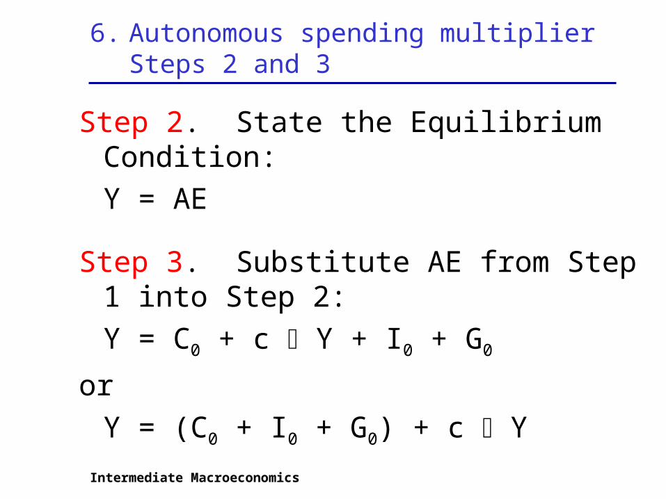
6. Autonomous spending multiplierSteps 2 and 3

Step 2. State the Equilibrium Condition:

Y = AE

Step 3. Substitute AE from Step 1 into Step 2:

Y = C0 + c Y + I0 + G0

or

Y = (C0 + I0 + G0) + c Y


6. Autonomous spending multiplierStep 4. Solve for National Income (Y)

Y = (C0 + I0 + G0) + c Y

Y - c Y = C0 + I0 + G0

(1 - c) Y = C0 + I0 + G0

Y = 1 (C0 + I0 + G0) 1 - c


6. Autonomous Spending Multiplier

Change in Y = Multiplier Change in C0, I0,or G0

Equilibrium model solution:

Y = 1 (C0 + I0 + G0) 1 - c

Autonomous Spending Multiplier:

1 or 1 1 - c 1 - MPC


7. Government Fiscal Policy

Given Equations:

AE = C + I + G + NX

C = C0 + c YD

I = I0, G = G0, NX = 0

YD = Y - t Y - T0 + TR

YD = disposable incomet Y = income tax revenuesT0 = lump sum taxTR = gov’t transfer payments


7. Government Fiscal PolicyStep 1. Restate aggregate expenditures

AE = C + I + G + NX

= C0 + c YD + I0 + G0

= C0 + c (Y - t Y - T0 + TR) + I0 + G0

= C0 + I0 + G0

+ c Y - c t Y - c T0 + c TR


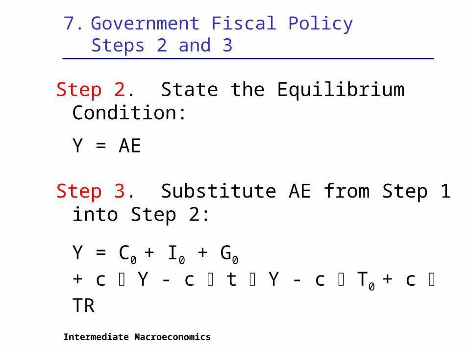
7. Government Fiscal PolicySteps 2 and 3

Step 2. State the Equilibrium Condition:

Y = AE

Step 3. Substitute AE from Step 1 into Step 2:

Y = C0 + I0 + G0

+ c Y - c t Y - c T0 + c TR


7. Government Fiscal PolicyStep 4. Solve for National Income (Y)

Y = C0 + I0 + G0 + c Y - c t Y - c T0 + c TR

Y = C0 + I0 + G0 - c T0 + c TR + (c - c t) Y

Y = C0 + I0 + G0 - c T0 + c TR + c (1 - t) Y

Y - c (1 - t ) Y = C0 + I0 + G0 + c (TR - T0)

[1 - c (1 - t )] Y = C0 + I0 + G0 + c (TR - T0)

Y = 1 [C0 + I0 + G0 + c (TR - T0)]

[1 - c (1 - t )]


7. Government Fiscal PolicyMultipliers

No Income

Tax (t = 0.0)

Income Tax (t = 0.3)

Autonomous Spending

1 = 5 1 - c

1 = 2.3 1 – c (1-t)

Transfer Payment

c = 4 1 - c

c = 1.8 1 – c (1-t)

Lump Sum Tax

- c = - 4 1 - c

- c = - 1.8 1 – c (1-t)

Assume c (marginal propensity to consume) = 0.8


7. Government Fiscal PolicyBalanced budget multiplier

• $1 increase in government spending

matched by

• $1 increase in lump sum taxes


7. Government Fiscal PolicyBalanced budget multiplier

• Spending multiplier (assume no income tax) 1 1 – c

• Lump Sum tax multiplier- c 1 - c

• Balanced budget multiplier: spending multiplier – lump sum tax multiplier

1 - c = 1 – c = 11 – c 1 – c 1 - c


7. Government Fiscal PolicyBalanced Budget Multiplier

From Step 4 (assume t = 0):

Y = 1 [C0 + I0 + G0 + c (TR - T0)] 1 - c

Multiplier (assume C0 = I0 = TR = 0):

Y = 1 ( G0 - c T0) 1 - c

Balanced Budget ( G0 = T0):

Y = 1 ( G0 - c G0) 1 - c = 1 ( 1 – c) G0

1 - c = 1 G0

Multiplier = 1


8. Automatic Stabilizers

Economy Moves Into

Recession Inflation

Desired Policy Government Spending Increase Decrease

Taxes Decrease Increase

Actual Outcomes

G - Defense Spending n/c n/c

TR - Social Security Benefits n/c n/c

TR – Unemployment Comp. Increase Decrease

TA – Lump Sum Tax n/c n/c

t Y - Income Tax Receipts Decrease Increase

intermediate macroeconomics chapter 5 the keynesian model

Documents