4/5/2018

1

INTERNATIONAL EQUITY MARKETS

General Overview and Differences

• Differences

- Macrostructure

- Liquidity

- Taxes

- Indexes

- Microstructure

- Organization

- Trading Procedures

4/5/2018

2

Liquidity

Liquidity

“Ability to buy or sell significant quantities of a security quickly, anonymously, and with minimal or no price impact.”

=> Most important attribute for an asset.

• Usual measures are:

1. Capitalization/GDP

2. Transaction size (market turnover)

3. Degree of concentration

4. Bid-ask spread

5. Number of non-trading days

6. Number of zero-return days

1. Capitalization/GDP

Fact: U.S. stock market is very large compared to the U.S. economy. See figures in Dec. 2014 USD.

Market Market Cap (MC) GDP (nominal) MC/GDP

U.S. 26,240 B 17,416 B 151%

China 6,005 B 10,355 B 57%

Japan 4,378 B 4,770 B 92%

U.K. 6,370 B 2,847 B 224%

India 3,324 B 2,047 B 162%

Brazil 844 B 2,244 B 37%

But, this number may not be a good indicator: for South Africa, in 2009, the MC/GDP was over 170%.

Also, this figure changes a lot. The MC/GDP for Brazil in 2009 was close to 50% and in 2007 was close to 100%.

4/5/2018

3

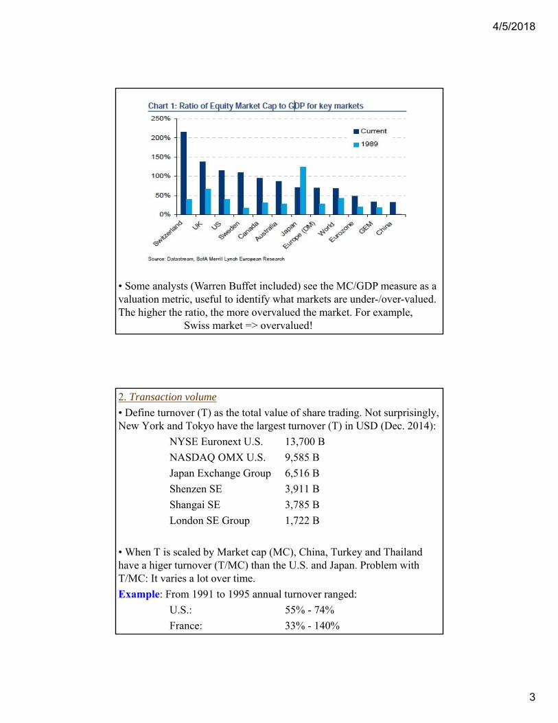
• Some analysts (Warren Buffet included) see the MC/GDP measure as a valuation metric, useful to identify what markets are under-/over-valued. The higher the ratio, the more overvalued the market. For example,

Swiss market => overvalued!

2. Transaction volume

• Define turnover (T) as the total value of share trading. Not surprisingly, New York and Tokyo have the largest turnover (T) in USD (Dec. 2014):

NYSE Euronext U.S. 13,700 B

NASDAQ OMX U.S. 9,585 B

Japan Exchange Group 6,516 B

Shenzen SE 3,911 B

Shangai SE 3,785 B

London SE Group 1,722 B

• When T is scaled by Market cap (MC), China, Turkey and Thailand have a higer turnover (T/MC) than the U.S. and Japan. Problem with T/MC: It varies a lot over time.

Example: From 1991 to 1995 annual turnover ranged:

U.S.: 55% - 74%

France: 33% - 140%

4/5/2018

4

2. Transaction volume

• Turnover as a percent of market capitalization (T/MC) in 2013:

3. Degree of concentration found in the major markets

• Composition: Many small firms vs. concentrated in a few large firms.

Institutional investors dislike small firms for fear of poor liquidity.

A concentrated market provides fewer opportunities for risk diversification and active portfolio strategies.

Example: Market share of the 10 largest companies.

U.S. 11.9%

Japan 20.2%

U.K. 23.2%

Germany 39.2%

Switzerland 67.0%

Netherlands 74.3%

4/5/2018

5

4. The bid-ask spread

Market maker buys shares (at the bid quote) and expects to sell those shares in the future (at the ask quote).

The longer it takes to receive a buy order The higher the required compensation Higher compensation Higher bid-ask spread.

An average bid-ask spread is a useful market liquidity indicator.

Example: The average bid-ask spread in the U.S. is 0.6%, while in Thailand the average bid-ask spread is 5.14%.

Problem with this measure: Not easy to obtain –definitely, not in Reuters, Bloomberg, or the WSJ.

5. Non-trading days

Market may be seem liquid on average, but there is no volume during some days. The number of non-trading days gives us an idea of liquidity.

6. Zero-return Days

Two things behind a no change in the price –i.e., zero return:

- No information

- No trading (stale prices) proxy for non-trading days

It is an easy measure to gather, just from stock prices.

Conclusion: Take a look at several liquidity indicators.

4/5/2018

6

Example: Liquidity -- The Case of Emerging Markets

Organization

Three market structure types: ○ Public exchange

○ Private exchange

○ Banker exchange

The private exchange

Origin: XVII and XVIII century's European commodity markets.

- Private institution with some government supervision.

- Brokers are created by independent members.

- Brokers compete among themselves or enjoy monopoly.

Private exchanges may compete within the same country (U.S., Japan, China, India).

Commissions: Negotiated or imposed by exchange or local law.

Example: U.S., U.K., Canada, Japan, Mexico, Argentina.

4/5/2018

7

The public exchangeOrigin: legislative work of Napoleon I. - Public institution.- Brokers are appointed by the government.- Brokers enjoy a monopoly over all transactions.

Brokerage firms are private.New brokers are proposed to the state by the broker's association. Commissions: fixed by law.

Examples: Belgium, Italy, Greece, and some Latin American countries.

The bankers exchangeOrigin: German tradition.- May be either private or semipublic organizations.- Brokers are banks.- Members must deal through the exchange.

In some countries, banks are the major securities traders.In Germany the Banking Act grants a brokerage monopoly to banks.

Examples: German sphere of influence: Austria, Switzerland,Scandinavia and the Netherlands.

4/5/2018

8

Recent Trends1) Deregulation: The private stock exchange is the norm. Many exchanges have become business organizations, listed in their own exchanges.

Example: Paris Bourse, Deutsche Börse, NYSE.

2) Consolidation: Competition has created consolidation: - OMX: OM & Stockholm Exchange (OMX) (1998); Helsinki (HEX) (2003); Copenhagen SE (KFX) (2005); Oslo SE (2006); Iceland SE (2006); Armenian (Armex) (2007) - NASDAQ buys PHLX and OMX (2007, 2008).- Euronext: Paris Bourse, Amsterdam (AEX) & Brussels (BXS) (2000); LIFFE (2002); Lisbon (BVL) (2002).- NYSE buys Euronext (2006).- CME buys CBOT (2006)- Toronto (TSX) & Montreal (MX) (2007)

Differences in Trading Procedures

The most important differences are in the trading procedures.

(1) Cash versus futures markets

(2) Fixed versus continuous quotation

(3) Computerization

(4) Internationalization

4/5/2018

9

(1) Cash versus futures markets

• Cash markets

Stocks are traded on a cash basis (settlement within a couple of days).

For more leveraged investments: Margin trading is available.

Margin trading: Investors borrow money from a broker.

A cash market transaction: a third party steps in.

Note: Margin trading is costly and, sometimes, difficult.

• Futures or forward stock markets

Provide an organized exchange for levered stock investment.

Forward stock markets compete with cash stock markets.

(2) Fixed versus continuous quotation

• Continuous market: transactions take place all day.

- Large market-makers assure liquidity.

- In some markets, the market maker has a monopoly for a given security, as is the case for the specialist on the NYSE.

- In other markets, the market makers (dealers or jobbers) compete

to provide the best quote.

• Fixed market: Transactions take place only at specific times.

- Call or fixing market: a single price applies to all transactions.

- Auction market: an asset is traded only few times per day and its price is determined through a competitive auction system.

4/5/2018

10

(3) Computerization

• Traditional trading method: floor trading.

- Traders meet on a floor to trade and to execute orders according to a set of pre-specified rules.

- Floor trading has been greatly influenced by computers: computers help to make floor trading cheaper, with fewer mistakes and faster.

• New trading method: computerized trading.

- A computer executes orders according to a set of pre-specified rules.

- Computerized trading allows the automated execution of orders entered by traders in their office.

- Best known system: Computer Assisted Trading System (CATS) -TSE.

- CATS eliminated the need for a floor where participants meet.

• Mixed system: NASDAQ.

(4) Internationalization• Traditional internationalization: International network of offices.

• New trend: Electronically access foreign markets. cheaper alternative.

Key to this new trend: Harmonization of electronic trading platforms

Examples:

(i) OMX: OM Stockholm Exchange (SSE), Copenhagen SW (CSE),Helsinki SE (HSE), the Iceland SE. (September 2006).

(ii) Euronext: Amsterdam SE, Brussels SE and Paris Bourse (Sep 2000)

(iii) NYSE Euronext: NYSE and Euronext (April 2007)

(iv) NASDAQ OMX: NASDAQ and OMX (February 2008)

International Exchange of the Future: Stock exchanges with their ownautomated trading system available worldwide on a 24-hour basis.

4/5/2018

11

Practical Aspects

Dual Listing

Fact: Some firms are traded on more than a dozen markets.

Implication: Shares should sell at the same price all over the world, once adjustment for exchange rates and transactions costs are made.

Procedures for admitting foreign stocks to local markets:

Montreal: Listed by simply by meeting the same regulatory requirements as those in its own jurisdiction.

U.S.: Must satisfy the local exchange and regulatory requirements.

Q: Why do companies double list?

Advantages of double listing:

- Easier access to foreign capital.

- Diversified ownership reduces the risk of a domestic takeover.

- Fragmented markets.

- Advertising.

Main disadvantage: Increased volatility.

Example: Situation: Bad political news in Chile.

Foreign investors tend to immediately sell their shares, driving domestic share prices down in this illiquid stock market.

Chilean investors have a less volatile behavior: They are not as shaken by domestic news, and have few investment alternatives. ¶

4/5/2018

12

American Depositary Receipts (ADRs)• Special shares for foreign company: depository receipts.

Many DR programs around the worldU.S.: American depository receipts (ADRs). U.K: Global DRs (GDRs). Singapore: Singapore DRs.

Simple process: (1) Foreign shares are deposited with a trust company.(2) Trust issues DRs.

To avoid unusual share prices, ADRs may represent a combination or a fraction of several foreign shares.

Example: Petroleo Brasileiro (Petrobras) ADR (PBR)JP Morgan has a 10 million shares of PBR in deposit. JP Morgan issues 5 million depository receipts (DR). Each DR represents 2 Petrobras shares. ¶

• Trading in ADRsTrading in ADRs avoids delays of trade settlement, problems with safeguarding, and making currency transactions.

Note: ADRs do not eliminate currency risk or country risk.

Example: BRL depreciates sharply, Petrobras (PBR) USD CFs decrease Petrobras ADRs will decline.

• There are more than a 2,700 ADRs available to U.S. investors.Representing over 80 markets. China has 124 ADR programs.

• ADRs account for more than 15% of the entire U.S. equity market.

4/5/2018

13

ADRs Trading Volume: Exchange Listed ADRs

• Types of ADRs(1) Listed ADRs (Level II and Level III): companies should meet all the exchange requirements. In December 1995, there were 316 Listed ADRs: 199 traded on the NYSE, 7 on the American Stock Exchange, and 110 on the NASDAQ.

(2) Unlisted ADRs: The rest of the ADRs trade on the OTC market(OTC level I), or privately placed (ADR Rule 144-A, or RADR).

- OTC Level I (pink sheets): Simplest way to access capital in the U.S.A Level I DR programme does not have to follow U.S. GAAP, nor it hasto make a full disclosure to the SEC.

- RADR: They are privately sold and bought by qualified institutionalbuyers (QIBs). QIBs include institutions that manage at least USD 100million.

Example: KIA Motors, LG Electronics, Samsung are all 144-A ADRs

4/5/2018

14

Examples ADRs in the U.S.:

AUSTRALIA: BHP (NYSE), Foster’s (OTC), Qantas (OTC)

BRAZIL: AES Tiete (OTC) AMBev (NYSE), CVRD (NYSE), VIVO (NYSE)

CHINA: Air China (OTC), Agria Corp. (NYSE), Baidu (NASDAQ)

CHILE: Concha y Toro (NYSE), LAN Airlines (NYSE), Enersis (NYSE)

EGYPT: Orascom Construction (OTC), Orascom Telec (OTC), Suez Cement (OTC)

FINLAND: Neste Oil (OTC), Nokia (NYSE), Stora Enso (OTC), UPM (OTC)

FRANCE: GDF Suez (OTC), France Telecom (NYSE), L’Oreal (OTC)

GERMANY: Allianz (NYSE), BMW (OTC), SAP (NYSE)

GREECE: Alpha Bank (OTC), Hellenic Petrol (NYSE), Hellenistic Telecom (NYSE)

JAPAN: Canon (NYSE), FujiFilm (NASDAQ), Hitachi (NYSE)

KOREA: Korea Electric Power (NYSE), Pohang Steel (NYSE), SK Telecom (NYSE)

MEXICO: Am Movil (NASDAQ), Cemex (NYSE), Femsa (NYSE), Telmex (NYSE)

NETHERLANDS: AKZO Nobel (OTC), ING (NYSE), Crucell (NASDAQ)

RUSSIA: Gazprom (OTC), Lukoil (OTC), Mechel (NYSE), Mosenergo (OTC)

TURKEY: AKBank (OTC), Koc Group (OTC), Petrol Ofisi (OTC), Turkcell (NYSE)

UK: Barclay’s (NYSE), BP (NYSE), British Airways (OTC), Imperial Tobacco (OTC)

Exchange Traded Funds (ETFs)ETFs are like open-ended mutual funds except that they can be bought and sold on an exchange like ordinary stocks.

An ETF holds assets: stocks, commodities, bonds, etc. Most ETFs track an index, such as the S&P 500, the MSCI EAFE or the MSCI Korea.

Relative to mutual funds, ETFs are attractive: low costs and liquidity.

ETFs have had phenomenal growth since inception in 1993 (SPDR).

4/5/2018

15

Exchange Traded Funds (ETFs)Global EFT Market (2008-2016) + Forecasts: Total Assets by Year.

Exchange Traded Funds (ETFs)US EFT Market: Listings and Market Cap by Year.

4/5/2018

16

Financial Analysis and Valuation

• Nothing unique to financial analysis in an international context.

Example: The methods and data required to analyze U.S.-, Mexican, or Malaysian-type manufacturers are the same. ¶

A research report on a company should include:

(1) Expected return.

(2) Risk sensitivity.

The information problemA firm is typically valued in two steps: (1) Forecast future earnings (EPS -expected earnings per share)(2) Assessment of how the stock market will value these forecasts. (PE -price-earnings ratio)

InformationU.S.: Firms publish their quarterly earnings.

Europe and Far East: Firms only publish their earnings once a year.

• Quality of the disclosed information: Varies from country to country. There is a market for companies "interpreting" for international investors the local books of companies:

Many international brokerage houses provide analysts' guides.

4/5/2018

17

Comparative analysis.Another difficult problem due to: - Different accounting principles- Different cultural, institutional and tax differences

Example: Swiss firms stretch the definition of a liability. They tend to overestimate contingent liabilities when compared to U.S. firms.

Example: German firms create hidden reserves often equal to 100% of fixed assets. Inventories tend to be understated.

Major differences in international accounting practices:

* Publication of consolidated statements* Publication of accounts corrected for fiscal distortion* Inflation accounting* Currency adjustment* Treatment of extraordinary expenses* Existence of "hidden" reserves* Depreciation rules* Inventory valuation

• Misunderstanding asset values and reported profits played a major role in the 1997 Asian crisis.

4/5/2018

18

• The lack of uniform accounting standards is costly. - International banks and investors charge higher interest rates to

companies that do not adjust follow U.S. or International standards. - Many firms do not have access to international capital markets because

their national accounting standards distort valuations. Japan ranks below Spain and South Korea on access to international capital markets.

• Cross-country research by Fan and Wong (2002) and Leuz et al. (2003) suggests that managers smooth earnings to create opacity to allow expropriation of assets.

• Opacity and information asymmetry reduce the willingness of investors to trade and, thus, to increase the liquidity premium.

Lang et al. (2009): In 21 EAFE markets, moving from the 25th to 75th transparency percentile is associated with a 40% decrease in the median bid-ask and a 17% reduction in the number of non-trading days.

ConvergenceThe dream of insurance companies, investors, bankers and regulators.

• Ongoing conversation about converging accounting standards between the International Accounting Standards Board (IASB), based in London, and the Financial Accounting Standards Board (FASB), based in the U.S.

The IASB sets and promotes the International Financial Reporting Standards (IFRS). The FASB caters to the development of U.S. GAAP.

IFRS is a more principles-based approach as opposed to GAAP, which is more rules-based. IFRS allows more flexibility (judgement, experience).

Most of the world follows IFRS. Seay (2014): the “gold standard.”

Changing accounting standards in the U.S. would be costly. Lin (2013) estimates that the cost of a full switch to be between 0.5% to 1% of annual revenues. USD 40-60 billion for companies in the S&P 500.

4/5/2018

19

Progress towards convergence has been done in many of those areas.

Big remaining issue: Inventory valuation. IFRS does not allow the last-in-first-out (LIFO) method. Reed and Pence (2013), the LIFO method isused by 36% of companies. LIFO tends to inflate costs and lower taxes.

Company Valuation

Companies are valued by discounting cash flows (DCF models). Thereare different ways to do this. The data needed for the DCF process:⋄ CFs to the firm (including periods of high growth and their duration).⋄ Expected growth from expansion.⋄ Discount rate.

In the usual DCF valuation process, risk is introduced through thediscount rate (k=r).

We will discuss three company valuation methods:(1) Dividend Discount Model (DDM)(2) Discounting Free Cash Flows(3) Valuation by PE Multiples

4/5/2018

20

Company Valuation - (1) Discounted Dividend Model (DDM)

• DDM is used to estimate the expected return on an investment:The value of an asset is determined by discounted the stream of cashflows it generates for the investor.

• DDM: Stock price (P) = Stream of discounted forecasted dividends.P = D1/(1+r1) + D2/(1+r2)

2 + D3/(1+r3)3 + D4 /(1+r4)

4 + ...

• A typical DDM approach is to decompose the future in three phases:1) Near future (next two years): Earnings are forecasted individually.2) Second phase (years two to five): A general growth rate for the

company's earnings is estimated. (revert to industry?)3) Third phase: A growth rate in earnings is supposed to revert to the

average of all (similar) firms in the market.

Dt-forecast's and P are known solve for the expected return (r).

Problems:- Companies have discretion over their dividend payments.

- International comparisons are difficult:Payout ratios vary considerably: The U.S. has a much lowerpayout ratio than the U.K.

- We need a model to calculate r. For example, the CAPM or the 3 Factormodel of Fama-French.

Example: It is Dec 1995. We want to value the expected return of theArgentine ADR YPR, based on the DDM. Since the cash flows wediscount are USD dividends, the discount rate should be a USD rate.

According to the CAPM, we should estimate E[return] in USD:E[rYPF] = rf + ßYPF E[rm-rf]

4/5/2018

21

Example (continuation):Data needed:ßYPF=.91 - estimated using a regressionrf =.085 - long-run governemt (“risk-free”) USD interest ratesE[rm - rf] =.095 - in USD, estimated using a long history.

E[rYPF] = .085 + .91 x (.095) = .17145 (in USD). ¶

Note, if we want to discount ARS dividends, we need to translate theE[rYPF] to ARS. Then, we adjust the discount rate using IFE:

(1 + rARG) = (1 + rUS) (1 + E[s])

To forecast currency movements, we usually rely on PPP. For example,E[s] ≈ (1 + IAR )/(1 + IUS) - 1.

Note: If inflation rates are small, we can use linearized PPP. Simarly, ifrates of returns are small, we can use linearized IFE.

Example: Using DDM to calculate the fair value of YPF ADRs.It is December 1995.

We need input values for Dt, rt, and St. t = 1996, 1997, 1998, ....PYPF-ADR = USD 20.53. (Market price at NYSE)St= 1 USD/ARS.

Dt = ? t = 1996, 1997, 1998, ....D1996

F = ARS .84.dt

F = 9.1% t = 1997, 1998, 1999.dt is low for international standards dt should increase in the future:dt

F = 15.7% t = 2000, ...

• rt = ? t = 1996, 1997, 1998, ....According to CAPM, we should estimate: E[rYPF] = rf + ßYPF E[rm - rf].Data:ßYPF=.91; rf =.085; E[rm- rf]=.095. <= In USD!

E[rYPF] = .085 + (.095) x .91 = .17145.

4/5/2018

22

Example (continuation): YPF ADR Valuation• St = ? t = 1996, 1997, 1998, ....st = -1% t = 1997, 1998, 1999.st = -2% t = 2000, ....

• Valuation Process:(1) Determine the USD PV of CF from 1996 - 1,999 (year 4), P1-4.- Effective USD rate of dividend growth from 1997 until 1999 is:[(1.091)x(.99) - 1] = .08009.- P1-4 = .84/(1.17145) + .84*(1.08009)/(1.17145)2 + .84*(1.08009)2/(1.17145)3 ++ .84*(1.08009)3/(1.17145)4 = USD 3.5559.

(2) Determine the USD PV of CF from 2000+ (year 5+), P5+.- The discounted dividends per share in year 4 will be:USD .84*[(1.091)x(.99)]3/(1.17145)4 = USD .56204.- The effective USD rate of div growth is [(1.157)x(.098) - 1] = .13386.- The USD PV of all futures cash flows after year 5 is given byP5+ = USD .56204 x (1.13386)/[(.17145 - .13386)] = USD 16.9533

Example (continuation): YPF ADR Valuation

(3) Add (1)+(2) -- Present value of a YPF ADR is:- P = P1-4 + P5+ = USD 3.56 + USD 16.95 = USD 19.50.

Market Price (NYSE) in December 1995 = USD 20.53.

It indicated that the YPF ADR was slightly overvalued, given ourestimates from the DDM. ¶

4/5/2018

23

Company Valuation - (2) Discounting Free Cash Flows

Alternative method to the DCF model: Discount free cash flows. The usual formula for calculating free cash flow is:

Free CF = EBITDA – Taxes - WC – Capital Expenditures

Once Free CFs are calculated for different years, they are discounted using the weighted-average cost of capital (WACC), kc:

kc = kWACC = ke (E/V) + (1-t) kd (D/V),

ke: cost of equity (usually, risk-adjusted, based on a model, say CAPM).

kd: before-tax cost of debt (usually, it is an interest rate or bond’s YTM),

t: marginal tax rate,

E: Market value of the company’s equity,

D: Market value of the company’s debt

V: Market value of the firm (=E+D).

• Weighted Average Cost of Capital

An alternative approach is to discount free CFs using the WACC (as discussed in Chapter X), where free cash flows are defined as:

Free cash flows = EBITDA – Taxes - WC – Capex,

where EBITDA represents earnings before interest, taxes, depreciation and amortization, Taxes represents taxes after interest deductions, WC represents change in net working capital, and Capex represents capital expenditures already planned.

These free CFs represent the CFs available to the shareholders and creditors after all expenses, payments to government, and necessary maintenance investments have been made.

Then, the free CFs are discounted using the WACC, kc:

kc = kWACC = ke (E/V) + (1-t) kd (D/V).

4/5/2018

24

Company Valuation - (3) Valuation by Multiples (Relative Valuation)

This is the most popular method, where firms, bonds, etc. are valuebased on how similar firms/bonds/etc. are priced by the market.

Relative valuation is done using multiples for “comparable firms.” Wesay firm A is cheap if it trades at 5 times earnings when comparablefirms B & C trade at 20 times earnings.

The key to this approach is defining comparable firms.

Usual multiples: Earnings, Book Value, Sales, Sector specific units(original visitors at internet sites, subscribers, members), etc.

Usual definition of comparable: Similar CFs, growth potential, & risk.

Note: Since not two firms are the same, ad-hoc adjustments are common.

Company Valuation - (3) Valuation by Multiples (Relative Valuation)

We will derive an “equilibrium (P/E) multiple” by deriving a fair (steadystate) value for a company. We will use a simple DCF model.

Calculation of the fair value of a company needs to inputs:

1) Discount Rate for firm j (rj):

rj = bond yields (risk-free) + risk premium for firm j.

Example: For well-established markets, real bond yields are about 3%.No consensus about the risk premium: From 0% to 12%.

2) Cash flows for firm j.

We will discount free cash flows, measured by Earnings (=E):

E=After interest, tax & capex, but before depreciation and amortization.

Adjustments to E: Firms re-invest earnings to replace assets & to expand.

4/5/2018

25

Company Valuation - (3) Valuation by Multiples (Relative Valuation)

Assumptions:

(A) Two downward adjustments (1/3 of earnings, E):

(1) Cost of replacing worn-out assets is higher than original (10%)

(2) Companies invest also to expand (≈25%).

(B) Earnings grow at rate g.

• Now, we can calculate fair value stock prices:

P = CF1/(1+r) + CF2/(1+r)2 + CF3/(1+r)3 + ....,

where CFt = 2/3 Et.

Et = E*(1+g)t

P = 2/3 E*(1+g)/(1+r) + 2/3 E*(1+g)2/(1+r)2 + 2/3 E*(1+g)3/(1+r)3 ...

This formula simplifies to:2/3 E∗[(1+g)/(1+r)]

1 − (1+g)/(1+r)

We will apply valuation by P/E multiple to the overall market. Assumptions:

(1) E = Corporate Earnings (Recall, CF = 2/3 E)

(2) Corporate earnings (E) grow at the rate of the economy –i.e., trend economic growth.

Example: It is 2017. Calculating the steady state P/E for the US market.

Data:

(1) Real economic trend growth (g) is 2.5% a year.

(2) Real bond yield is 3% (=rf)

(3) Risk premium is 3%. (≈ β E[rM - rf])

From (2) and (3) r = discount rate = 6%.

2/3E [(1+g)/(1+r)][1 −(1+g)/(1+r)].

2/3 [1.025/1.06][1 − (1.025/1.06)] = 19.52

4/5/2018

26

Example (continuation):

P/E = 19.52 < P/ESP500 (trailing) = 24 (in 2017) U.S. over-valued!

Note: Based on 1870-2017, average P/E is 16.8 U.S. under-valued! ¶

Problem: Global economy is not in a steady state. Growth rates change over time: Over the business cycle, profits take different proportions of the GNP.

Example: When countries are in the advanced stages of the business cycle, wages rise at a faster pace. P/E ratios have to be adjusted.

Example: Ad-hoc adjustments.

U.S. economy: late stages of the business cycle.

Adjust steady state P/E by .80.

Asian Pacific Countries: room for improving the efficiency of firms.

Adjust steady state P/E by 1.10. ¶

• PE Values for S&P Index

Note: Average (1870-2017) P/E = 16.8 2017 P/E is 42% higher.

Similar behavior in the U.K. P/E for FTSE 100 = 33 > Average P/E =15.

4/5/2018

27

• PE Values for S&P Index - Adjustments

Why Go International?

• Diversification

If it is good to diversify in domestic markets, it is even better to

diversify internationally.

4/5/2018

28

Q: Why does the frontier move in the NW direction?

A: Low Correlations! Low correlations are the key to achieve lower risk.

• Empirical Fact #1: Low Correlations

The correlations across national markets are lower than the correlations across securities in most domestic markets.

Return correlations are moderate to low (many lower than .50).

There is a regional effect:

Correlations between neighboring markets tend to be higher: Correlation between the US and Canada is .74; US and Japan is .36. (Data: 1970-2015).

TABLE X.1MSCI Indexes: Correlation Matrix (1970-2015)

A. European Markets

International returns correlations tend to be moderate, with an average of 0.45 (Table X.1). Neighboring countries show higher numbers.

MARKET Bel Den France Gerrn Italy Neth Spain Swed Switz U.K. Wrld

Belgium 1.00 0.59 0.72 0.70 0.54 0.75 0.56 0.55 0.68 0.59 0.69

Denmark 1.00 0.53 0.59 0.48 0.62 0.51 0.54 0.55 0.49 0.61

France 1.00 0.73 0.59 0.73 0.59 0.57 0.68 0.63 0.73

Germany 1.00 0.56 0.78 0.58 0.64 0.71 0.54 071

Italy 1.00 0.55 0.57 0.50 0.50 0.57 0.57

Netherlands 1.00 0.59 0.63 0.75 0.69 0.81

Spain 1.00 0.57 0.50 0.47 0.62

Sweden 1.00 0.57 0.52 0.69

Switzerland 1.00 0.62 0.72

U.K. 1.00 0.73

World 1.00

4/5/2018

29

• Empirical fact 2: Correlations are time-varying

International correlations change over time. They can have wild swings.

General finding: During bad global times, correlations go up

=> when you need diversification, you tend not to have it!

• Empirical fact 2: Correlations are time-varying

Correlations change over time: Also between U.S. stocks, but not as much as international correlation. Note also they are higher!

4/5/2018

30

• Empirical fact 2-A: Correlations seem to be increasing

Correlations have increased over the last 10 years.

- Germany and France have become the same asset!

Return Correlation: France and Germany

-0.20

0.20.40.60.81

1.2

Jan-72

Jan-74

Jan-76

Jan-78

Jan-80

Jan-82

Jan-84

Jan-86

Jan-88

Jan-90

Jan-92

Jan-94

Jan-96

Jan-98

Jan-00

Jan-02

Jan-04

Jan-06

Jan-08

Jan-10

Jan-122

-yr

Ro

llin

g C

orr

el

Return Correlation: Germany and EM

0.0

0.20.4

0.60.8

1.0

Jan-90J an-91J an-92Jan-93Jan-94Jan-95J an-96J an-97J an-98Jan-99Jan-00J an-01J an-02J an-03Jan-04Jan-05Jan-06J an-07J an-08J an-09Jan-10Jan-11Jan-12

2-y

r R

olli

ng

Co

rre

l

•Empirical fact 2-A: Correlations seem to be increasing

It also true at the domestic level. JPMorgan: “Correlation Bubble”

4/5/2018

31

• Empirical Fact 3: Risk Reduction

Past 12 stocks, the risk in a portfolio levels off, around 27%. Forinternational stocks, the risk levels off at 12%

• Empirical Fact 4: Returns Increase

Portfolios with international stocks have outperformed domestic portfolios in the past years. About 1% difference (1978-1993).

Q: Free lunch?

A: In the equity markets: Yes! Higher return (1% more), lower risks (2% less).

Q: How to take advantage of facts 2 and 3?

A: True diversification: invest internationally.

4/5/2018

32

Example: Higher Returns - The Case of Emerging Markets (EM)

Example: Lower Risk/Higher Returns!Taken from H. Markowitz’s “A Random Walk Down Wall Street.”

4/5/2018

33

Example: Lower Risk/Higher Returns II -The Case of EM

• Empirical Fact 5: Investors do not diversify enough

Many studies show that domestic investors tend to invest at home. In a 2002 UBS survey, the most internationally diversified investors are Netherlands (62%), Japan (27%) and the U.K. (25%).

=> The U.S. ranks at the bottom of list: only 11%.

More recent data (2010) shows better proportions. For example, the U.K. and the U.S. international allocations are 50% and 28%, respectively.

This empirical fact is called the Home Bias.

Proposed explanations for home bias and low correlations:

(1) Currency risk.

(2) Information costs.

(3) Controls to the free flow of capital.

(4) Country or political risk.

(5) Cognitive bias.

4/5/2018

34

• Things have improved. I started teaching this class in 1995. The amount invested internationally by U.S. investors was less than 7%, one of the lowest numbers in the world!

• Home bias everywhere: Even for Institutional investors (2013 data)

4/5/2018

35

Related Question: What should be your international exposure?- GDP weighted? Exposure to US: 25% to 30%

Related Question: What should be your international exposure?- GDP weighted?

4/5/2018

36

Related Question: What should be your international exposure?- GDP weighted?- Market cap weighted? Exposure to US: 27% to 33%

Explaining International Stock Returns

Risk-Return in International Markets

Recall that there is no agreement on an equity risk premium for developed markets. Things get more complicated when we introduced emerging markets. We do observe, as expected, high risk is correlated with high return. Table below shows returns from 1993-2017:

Market Return Stand Dev Sharpe Ratio

EM-Asia 7.24 24.13 0.1990EM-Latin America 10.65 27.68 0.2969

U.S. 8.72 14.25 0.4409U.K. 7.77 21.44 0.1411Japan 9.94 20.74 0.2506World 7.06 14.44 0.3207EAFE 5.48 16.06 0.1899

4/5/2018

37

Moments in International Markets

Higher moments association with risk:

- Standard deviation Volatility risk

- Skewness Crash risk

- Kurtosis Tail risk

Chang, Christoffersen, and Jacobs (2013) and Conrad, Dittmar, and Ghysels (2013) find that domestic stock traders are compensated when their cross-sectional domestic indices/stock portfolio returns have high volatility, low skewness, or high kurtosis.

Shu-Hsiu Chen (2018) finds similar results in international markets. He also tried to forecast returns next month using this month higher moments. He was successful in some markets (in particular, for both measures, Australia & Malaysia).

Moments in International Markets: 2007 – 2016 from Chen (2018)

CountryMonthlyReturn

Implied Volatility

Implied Skewness

Implied Kurtosis

Euro Area 0.0003 0.1057 -0.9016 6.6929Germany 0.0043 0.1669 -0.8655 7.2734France 0.0019 0.1493 -2.0033 11.4318Italy -0.0029 0.2463 -2.5396 15.1776UK 0.0001 0.2136 -1.5305 10.4403Australia 0.0031 0.1935 -1.1564 7.8827Switzerland 0.0035 0.1103 -1.0811 9.1301Japan 0.0017 0.1894 -3.1633 31.4871Sweden 0.0040 0.1460 -1.1022 7.4215Spain 0.0003 0.1467 -0.6460 5.8272Canada 0.0030 0.1402 -1.2425 8.3353Brazil 0.0045 0.1846 -0.6298 6.5996Mexico 0.0024 0.1575 -0.3518 4.1037Korea 0.0067 0.1679 -0.2389 3.3512Singapore 0.0042 0.2850 -2.5537 16.7907Malaysia 0.0038 0.2271 -1.8902 13.3735Taiwan 0.0044 0.1880 -2.0633 17.7618Hong Kong 0.0064 0.1687 -1.5824 11.8461US 0.0058 0.1936 -0.6456 9.8318

4/5/2018

38

Moments in International Markets

Forecasting one-month ahead international stock returns -Chen (2018).

CAPM in International Markets

There is a wide dispersion in expected returns in international markets, which the traditional CAPM (ß) cannot explain. Recall CAPM:

rjt – rft = αi + ß (rmt – rft) + εjt (Testing CAPM – H0: αi = 0)

Market Return Std Dev Sharpe Ratio

Brazil 16.58 37.54 0.3768China 5.40 33.25 0.0785Greece -0.18 35.46 -0.0736India 12.05 28.99 0.3318Malaysia 6.54 27.82 0.1477Mexico 10.00 27.75 0.2728Pakistan 6.79 34.91 0.1248Poland 18.62 44.78 0.3615Russia 22.65 50.09 0.4035South Africa 11.30 26.30 0.3373

U.S. 8.72 14.25 0.4409World 7.06 14.44 0.3207EAFE 5.48 16.06 0.1899

4/5/2018

39

Risk-Return in International Markets

Several papers try to explain these differences, among them:

⋄ Global economic risks −Ferson and Harvey (1994).

⋄ Currency risk −Dumas and Solnik (1995).

⋄ Inflation risk −Chaieb and Errunza (2007).

⋄ Momentum & global CF/P factors −Hou, Karolyi and Kho (2011).

⋄ Liquidity risk −Karolyi, Lee, & van Dijk (2012), Malkhozov, et al. (2014).

⋄ Investment restrictions −Karolyi and Wu (2014).

⋄ Regional Factors (mainly, Market & HML) −Fama-French (2015).

• Not a trivial matter: We use risk-return models to estimate the cost of equity (ke) and the cost of capital (kc).

Q: What kind of factors explain security returns?

(1) International

(2) Domestic

(3) Industrial

Domestic vs. International Factors

• We want to determine the relative importance of factors.

A: Separately correlate each individual stock with:

i. World sock index ( international factor)

ii. Appropriate industrial sector index ( international factor)

iii. Currency movement ( international factor)

iv. Appropriate national market index ( domestic factor)

B: Compare with all factors together. ( joint 4-factor model)

4/5/2018

40

Example: We regress each individual stock against each factor and obtain its R2.Average R2 of Regression on Factors

Single-Factor Model All FactorsMarket World Indust Curren DomesticBelgium .07 .08 .00 .42 .43Germany .08 .10 .00 .41 .42Norway .17 .28 .00 .84 .85Spain .22 .03 .00 .45 .45Sweden .19 .06 .01 .42 .43France .13 .08 .01 .45 .60Italy .05 .03 .00 .35 .35Netherlands .12 .07 .01 .34 .31U.K. .20 .17 .01 .53 .55U.S. .26 .47 .01 .35 .55Canada .27 .24 .07 .45 .48Australia .24 .26 .01 .72 .72Hong Kong .06 .25 .17 .79 .81Japan .09 .16 .01 .26 .33Singapore .16 .15 .02 .32 .33All .18 .23 .01 .42 .46 Domestic factors are the most important.

Currency factor almost negligible (hedging adds value?)

Fama-French Regional Factors in International MarketsFama-French (2012) tested their 3-factor model using Global factors:Global Market (rw – rf); Global SMB; & Global HML.

Finding: 3-factor global model does not explain international returns.

Fama-French (2015) tested a regional 5-factor model. They added to the3 standard factors (Market; SMB; & HML) a profitability factor (RMW:robust minus weak operating profitability); and an investment or stylefactor (CMA: conservative minus aggressive investments).

The regional model should explain returns of firm j in market i (i= NorthAmerica, Europe, Japan, Asia-Pacific):rjt – rft = αi + ß1 Mktit + ß2 SMBit + ß3 HMLit + ß4 RMWit+ ß4 CMAit+ εjt

Fama-French test the model using sorted portfolios (based on size, BM,OP and CMA).

4/5/2018

41

CAPM, 3- & 5-Factor Regional Factor Models: Test Model - H0: αi=0

From Sundqvist (2017, for Nordic stock data) – Sorts by Size-B/M (16 portfolios: Smallest & Lowest BM; Small 2 & Low BM 2; etc.):

Tests results: 3-factor model only one αi different from 0. Not bad!

CAPM, 3- & 5-Factor Factor Models: Test Model - H0: αi=0

From Sundqvist (2017, for Nordic stock data) – Sorts by Size-OP.

Tests results: Many αi’s different from 0. A problem for model! Similar results for Size-Inv.

4/5/2018

42

Findings: In general, the 5-factor model performs OK (better/not worsethan 3- & 4-factor model).

- Except for Japan, the value premium is larger for small stocks.

- Expected investment premium is larger for small stocks is stronger, at least for the two regions with the largest market cap (NA and Europe).

- Of the 4 nonmarket factors, HML returns of Europe and NA are most correlated (0.61). Next is CMA (0.57), SMB, or small minus big (0.31), and RMW (0.21). RMW is least correlated across regions (0.21 correlation for Europe and NA is the largest).

- HML is important for describing average returns in all regions.

- RMW is important for describing NA, European and AP average returns. (For Japan maybe a marginal role).

- The evidence for CMA is mixed. It works only in NA and AP.

- SMB seems redundant everywhere except NA.

- CMA may play the role of absorbing the low average returns of high-investment small stocks.

Fama-French Regional Factors in International Markets

From Fama-French (2015) – Test redundant factor: H0: Intercept=0.

4/5/2018

43

Valuation of MNCs• The extent of foreign operations for many MNCs raises the question:Can a portfolio of MNC stocks achieve true international diversification?A: No! MNCs do not provide all the benefits available from direct

investment in foreign securities.

Example: We examined firms from nine countries.ri = αi + ßUS rUS + ßNL rNL + ßBEL rBEL + ßGER rGER + ...

Nationality Multiple Singleof MNF Index Index

US GER FRA SWI UK R2 beta R2

Amer. MNF .94 -.01 .02 -.01 -.07 .31 1.02 .29German MNF .24 1.18 .10 -.15 -.11 .74 1.18 .65French MNF -.10 .18 .95 -.22 .03 .62 1.08 .45Swiss MNF -.12 -.09 -.11 1.74 .16 .75 1.39 .52British MNF -.10 -.09 -.09 .07 .84 .49 1.06 .44

Conclusion: MNC stock prices are more affected by domestic factors. ¶

Valuation of MNCs

Possible explanations of results:- National control- Management policy- Government constraints

4/5/2018

44

International Capital Market Integration

• Integration and The Pricing of Assets

Capital Market Integration: Assets in different currencies or countries display the same risk-adjusted expected returns.

Segmentation: The risk-return relationship in each national market is primarily determined by domestic factors.

• Tests for integration:

(1) Direct: Measure barriers to capital movements. (Be careful with loopholes).

(2) Indirect: Measure stock prices and compare them. (A better measure).

Q: Why do we care about International Capital Market Integration?

A: (1) Choice of raising capital in two countries.

(2) If segmentation, international portfolios should display superior risk-adjusted performance.

Country Funds

• Close-end funds (CEF) differ from open-end mutual funds: They neither issue nor redeem shares after IPO. To buy or sell shares, you have to go to the market.

• Each CEF provides two market-determined prices:

- The country fund's share price (P) quoted on the domestic market.

- Its NAV determined by prices of the underlying shares traded on the foreign market.

If P < NAV, closed-end fund sells at a discount.

If P > NAV, closed-end fund sells at a premium.

4/5/2018

45

• CEF Puzzle: Domestic closed-end funds, on average, sold at a substantial discount during the 70's and early '80s.

• Country CEF: Investment company that invests in a portfolio of assets in a foreign country and issues a fixed number of shares domestically.

Restrictions will raise P relative to its NAV by approximately the amount the marginal domestic investor is willing to pay to avoid them

Example: On January 13, 1989:

The Korea Fund's share sold at a 65% premium.

The Brazil Fund sold at a 35% discount. ¶

Restricted countries like Korea, Thailand and Taiwan sell at a premium. Less restricted countries like Germany and U.K. sell at a discount.

Statistics for Premiums for Closed-End Country Funds (1981-1989)

Fund or Portfolio Mean SD ρ1Brazil -28.82 9.64 .92Mexico -13.78 33.72 .97France -20.18 8.41 .92Germany -4.32 5.90 .77U.K. -21.37 6.74 .72Japan -11.73 10.50 .96Korea 44.35 20.86 .93Malaysia -7.46 19.75 .97Taiwan 40.96 36.24 .96Thai 25.46 12.45 .93Country Funds -4.54 11.88 .89Domestic Funds -11.22 5.58 .97

Example: The announcement of changes in investment restrictionsdecreased country fund premiums by an average of 6.8% in recent years.

Evidence favors International Market Segmentation: Financialrestrictions to foreign investment work.

4/5/2018

46

Linkages between Stock Markets

• The moderate to low correlation coefficients are a good argument internationally diversifying portfolios.

• The analysis of correlation coefficients might not be that a correct tool.

Example: Situation:

No movement of capital is allowed between national stock markets.

Common monetary policies induce positive correlations.

In such a case, ex ante, or expected, returns could be very different across markets, even with highly correlated ex post returns. ¶

The Crash of October 1987• Q: Why the October 1987 Crash is important?A: Only month during the 1980's where all the stock markets around theworld moved in the same direction.

• Q: How did the Crash start?A: The crash started in non-Japanese Asian countries and continuedthrough European markets, the U.S. and finally Japan.

The following Table reproduces the daily returns during the Pre-Crash Period, the Crash Period and the Post-Crash Period by Country

4/5/2018

47

Daily Returns (percent/day) by Country

Country 1/2/87-10/12/87 10/12/87-10/30/87 11/2/87-3/31/89

Australia .2239 (0.850) -3.5160 (8.315) .0475 (1.216)

Hong Kong .2218 (1.121) -5.4174 (12.072) .1083 (1.353)

Japan .1543 (1.274) -0.9777 (5.567) .0810 (0.946)

Malaysia .2821 (1.171) -3.6080 (6.026) .0128 (2.754)

N. Zealand .0291 (1.091) -2.0473 (5.296) -.0755 (1.366)

Singapore .2508 (1.075) -3.9675 (10.182) .1004 (1.327)

Austria -.0202 (0.736) -0.8255 (1.663) .0699 (0.557)

Belgium .0808 (0.814) -1.6531 (4.316) .0906 (0.965)

France .0114 (0.920) -1.6526 (4.568) .1018 (1.254)

Germany -.0296 (1.251) -1.5913 (4.178) .0254 (1.292)

Italy -.0338 (1.017) -1.3943 (3.184) .0293 (1.149)

Netherlands .0672 (0.993) -1.5985 (5.296) .0633 (1.301)

Spain .2143 (1.276) -2.4154 (3.286) .0555 (0.927)

Sweden .1272 (1.009) -1.8998 (4.534) .1202 (1.242)

Switzerland .0156 (0.917) -2.0706 (5.409) .0025 (1.305)

U.K. .1852 (0.865) -2.0759 (4.947) .0524 (0.962)

Canada .1143 (0.689) -1.5150 (5.413) .0405 (0.772)

Mexico .9831 (2.509) -3.4050 (6.892) .0128 (2.754)

U.S. .1213 (0.965) -1.4128 (7.253) .0428 (1.094)

Portfolio insurance and computer systems?Journalist and politicians blamed the Crash on a variety of sourceranging from portfolio insurance to inadequate computer systems.

• Finding: Claims totally unfounded. Many studies have found thatcountries with portfolio insurance crashed less that countries without it.

Futures markets?The argument seems to be that irrational speculators cause instability.

• Finding: Stock markets with related futures markets crashed in thesame way as countries without futures exchanges.

4/5/2018

48

Specific event?Search for a triggering event:(1) announcement on October 14 of a worse than expected trade balance.(2) poor performance of Asian markets in the week before the Crash.(3) introduction in the U.S. Congress of anti-takeover legislation.

• Finding: Last event is the most persuasive; however, it is difficult tobelieve that it had such a extraordinary effect in other markets.

Speculative bubble?Eugene Fama, Nobel Prize winner, says that the most fascinating aspectof 1987 was not the Crash itself, but the incredible market advanceduring the previous five years.

This apparent behavior has been attributed to a speculative bubble.Under this view, the most plausible theory for the Crash is that aspeculative bubble burst in October 1987.

Not easy to test this H0: Tests are complicated (usually, not linear).

• Finding: Several studies have dismissed it as a plausible explanationfor the October 1987 Crash.

4/5/2018

49

• Q: Can a Crash be avoided?

• The immediate consequence of the Crash was a couple of reports byofficial agencies with recommendations.

The proposed measures include:1. increase in margin requirements2. imposition of price limits3. differential taxing for short and long positions

• Finding: There is no evidence that margin requirements or price limitshave any impact on stock price volatility.

• Summary:- The Crash was an international event.- Markets with different regulations, controls, taxes and trading systems.- All experienced a significant negative shock on October 1987.

U.S. opening effectUse of daily data has a problem: overlapping trading hours.

Difficult for some markets to distinguish:Common movement (caused by world factors)Specific movement (caused by domestic factors)

Example: A positive co-movement between NY and London (they share2:30 hours of trading) might reflect common information or the influenceof one specific market in the other.

• Finding using intradaily data between NY and London: They onlyaffect each other around the time New York is opening (9:30 AM, EST).

4/5/2018

50

Big movements, higher correlationsWhen price changes are big, transaction costs become relatively unimportant. Transaction costs are a barrier for instantaneous arbitrage.

Big price changes will bring world markets together.

• Finding: Cross-market correlations tend to be positively correlated with measures of price volatility.

Application: High Volatility, Correlations and Portfolio Choice• The lower the correlation between the assets, the greater are the benefits due to diversification.

Empirical Fact: Recall the “Home bias."

• Changes in correlations will affect the composition of optimal portfolios.

• For the U.S. investor, the benefits of diversification change depending on the state of the volatility structure.

=> When you really want diversification (high domestic volatility), thebenefits are lower (high overseas volatility).

In Table X.7, the correlations between the U.S. and other major markets are calculated for two U.S. regimes: high volatility and low volatility.

4/5/2018

51

International Booms and Crashes

Taken from Goetzman (2015). Study of 21+ world markets 1900-2014 (annual data = 3,470 observations)

• Bubbles

Definition: A bubble is defined as a boom followed by a crash.

A crash is a large, rapid decline in market prices.

Q: What is large? A single year (or 3-yrs) of cumulative return of 100%

What is rapid? A a drop of at least 50% over the next 5 years.

- Boom: 8.33% of sample had 100%+ annual growth in 1-yr (72 mkt-yrs)

- After 1-yr - 4.17% of boom markets crashed

- After 5-yrs - 15.28% of boom markets crashed.

- 26.93% of boom markets had at least doubled again.

4/5/2018

52

- Boom: 14.06% of sample had 100%+ annual growth in 3-yr (460 mkts)

- After 1-yr - 4.57% of boom markets crashed

- After 5-yrs - 10.42% of boom markets crashed

- 21.73% of boom markets had at least doubled again.

Bust: 2.48% of sample has a -50% annual return in 1-yr- After 1-yr - 13.16% of bust markets doubled (10 mkts-years)- After 1-yr - 6.58% of bust markets crashed again (5 mkts-years)

Conclusions: - Stock market bubbles are rare.- The overwhelming proportion of price increases in global markets were not followed by crashes.

Interesting details:- Long-run return for 21 Developed Mkts (1900-2014): 12% (SD = 31%) - Long-run return for 20 EM (199+ - 2014): 11% (SD = 51%)