International Journal of Heat and Mass Transfer 80 (2015) 398–406

Contents lists available at ScienceDirect

International Journal of Heat and Mass Transfer

journal homepage: www.elsevier .com/locate / i jhmt

An improved model for predicting thermal contact resistanceat liquid–solid interface

http://dx.doi.org/10.1016/j.ijheatmasstransfer.2014.09.0480017-9310/� 2014 Published by Elsevier Ltd.

⇑ Corresponding author.E-mail address: Luoxb@hust.edu.cn (X. Luo).

Chao Yuan, Bin Duan, Lan Li, Bofeng Shang, Xiaobing Luo ⇑School of Energy and Power Engineering, Huazhong University of Science and Technology, Wuhan 430074, China

a r t i c l e i n f o a b s t r a c t

Article history:Received 17 June 2014Received in revised form 2 September 2014Accepted 13 September 2014

Keywords:Thermal interface materialsThermal contact resistanceLiquid–solid interfaceWettability analysis

Polymeric fluidic thermal interface materials (TIMs) are commonly utilized to reduce the thermal resis-tance between two solid surfaces in microelectronics. When filling TIMs between the solid surfaces, anamount of air is entrapped between the liquid and solid surfaces, resulting in a thermal contact resistance(Rc) arising at the liquid–solid interface. Rc plays an important role on the thin TIMs with high thermalconductivity, while analytical models for Rc at liquid–solid interface are scarce. Based on formerresearches, this paper developed an improved predictive model through conducting the wettability anal-ysis at the interface. The model expresses Rc as a function of topography of solid surface, wettability of theliquid on rough surface, mechanics of contact at the interface, and thermal parameters of the contactingbodies. Rc at the TIM-aluminium interface was measured for comparison with the model results. Thecomparison shows that the model results matches to experimental data within 14.3% when the appliedpressure is 0.1 MPa, and the deviations are still within the error bars at higher pressure.

� 2014 Published by Elsevier Ltd.

1. Introduction

Thermal interface materials (TIMs) are commonly used in thethermal management of microelectronics. Polymeric fluidic TIMs,such as thermal greases and phase change materials, are often uti-lized to reduce the thermal contact resistance (Rc) between the dieand the heat spreader, and between the heat spreader and the heatsink [1–3]. Although the polymeric TIMs with high thermal con-ductivity lead to low bulk thermal resistance (Rbulk), thermal resis-tance at the TIM bond lines is often higher than expected. One ofthe most important reasons is that when filling the polymeric flu-idic materials between the solid surfaces, an amount of air is nor-mally entrapped inside the microcavities of the rough solid surface,resulting in a Rc arising at the liquid–solid interface [1,4]. Rc playsan important role on the thin TIMs with high thermal conductivity[3], while good physical-based analytical models for Rc at liquid–solid surface are still lacking in literatures reviewed carefully inRef. [3]. It is therefore necessary to develop an effective model topredict it.

Past literatures abound with the models of Rc in solid–solid con-tact conditions [5–8]. These studies have all concluded that Rc is afunction of the surface roughness, asperity slope, mechanical

properties of the solid bodies, apparent area of contact and thecompressive load between the contacting surfaces. However, thesemodels are not suitable for the polymeric fluidic TIMs because themechanical properties, such as Young’s modulus or hardness, can-not be defined by the same way [4].

Two approaches have been used to predict Rc according to thelimited literatures. One way is to use a numerical model of heattransfer within the solid substrate and the liquid, and to accountfor temperature gradients within them [9–10]. Bennett and Pouli-kakos [9] developed a model for estimating thermal contact coeffi-cient between the molten metal and substrate, and they find thatthe pockets of entrapped air cause indentations on the bottom sur-face of molten metal. Liu et al. [10] also applied the numericalmethod to conduct thermal contact analysis for a molten metaldrop impacting on a substrate, their results suggest that the typeof substrate material effect the thermal contact coefficient a lot.The second way is to follow the method at the solid–solid contactconditions [5–8] to build theoretical models at the liquid–solidinterface by conducting topographical and mechanical analysesat the interface [4,11–12]. Prasher [4] developed a surface chemis-try model for the fluidic TIMs–solid contacts based on the defini-tion of Rc proposed by Madhusudana [13]. The advantage of suchmodel is taking into consideration the wettability of the liquidon rough surface and making mechanical analysis in detail. Thusthe model successfully illustrated the interface characteristics at

Nomenclature

as radius of microcontacts, mbs radius of heat flux tube, mBLT bond line thickness, mk thermal conductivity, W m�1 K�1

L distance between the marks, mm slope of real surface profilemn slope of modified surface profilens microcontacts density of solid surface, m�2

Pb applied pressure, PaPc capillarity pressure of liquid, PaP0 atmospheric pressure, Paq heat flux, W m�2

Ra arithmetic average of the surface roughness, mRbulk bulk thermal resistance of TIM, m2 K W�1

Rc thermal contact resistance, m2 K W�1

Rq root mean average of the surface roughness, mRsm mean peak spacing, mRtot total resistance at the TIM bond lines, m2 K W�1

rc thermal resistance of a single microcontact spot, K W�1

r2 correlation coefficientsT0 atmospheric temperature, KTc contact temperature at the liquid-solid interface, K

V0, Vc volume of the entrapped air before and after the liquid-solid contact, m3

Y height of the entrapped air after the liquid–solidcontact, m

Greekr standard deviation of the asperities heights, m/(y) Gaussian distribution function of the heights of

asperitiese factor related to the surface profilec surface energy, N m�2

h contact angle, degu angle between the cavity and mean plan, degDT temperature difference of the bond lines, KDR error in measurement of thermal resistance, m2 K W�1

DBLT error in measurement of BLT, mSubscript1, 2 Sidesd dispersion component of surface energyl Liquidp polar component of surface energys Solid

C. Yuan et al. / International Journal of Heat and Mass Transfer 80 (2015) 398–406 399

the liquid–solid contact. The surface geometry assumption in thismodel is that the solid asperities are conical in shape with thesame heights, and the spacing of the peaks and valleys is identicaland equal to the roughness sampling interval [4]. However rough-ness sampling interval is a profilometer parameter that is used tomodify the roughness measurement conditions [14]. On the otherhand, Hamasaiid et al. [11–12] developed a predictive model forthe casting-die interface based on the definition of Rc in CMYmodel [6]. The advantages of this model are assuming the asperityheights follow a Gaussian distribution which is more acceptable forexhibiting the surface geometry [6], and using mean asperity peakspacing (Rsm), measured by the profilometer, as the spacing of thepeaks and valleys. Different from surface chemistry model,mechanical analysis in Hamasaiid et al. model are completed byevaluating the capillarity pressure of the molten alloy as a functionof the applied pressure through experiments. Predictions of themodel are found to agree with the experimental results.

According to the above review, Hamasaiid et al. model is foundto have better topographical analysis, while wettability analysis inthe surface chemistry model makes it characteristic-based andsuitable for different types of liquid–solid interfaces. Thus the ideaof this paper is to develop an improved model based on Hamasaiidet al. model by adopting the wettability analysis at the liquid–solidinterface. This improved model is compared with the experimentalresults of Rc at the TIMs–solid interface.

Fig. 1. Formation of Rc and the resistance components in the solid–TIM–solidstructure.

2. Model of thermal contact resistance

2.1. Theoretical background

Fig. 1 schematically shows the formation of Rc at the fluidicTIM–solid interface. Heat flux passing from the solid to TIM or fromTIM to solid needs to be constricted at the microcontact spots. Atthe macroscopic scale, it brings in a temperature difference atthe interface resulting in a thermal resistance. Based on CMYmodel [6], the thermal field at the interface can be split into severalidentical isothermal flux tubes as illustrated in Fig. 1. The thermalresistance of a single microcontact spot can be determined fromthe following relationship [6]:

rc ¼1� as

bs

� �1:5

2ksasð1Þ

where ks = 2k1k2/(k1 + k2) is the effective thermal conductivity ofthe contacting bodies, as is the radius of the circular microcontactpoint and bs is radius of the heat flux tube. Considering the micro-contacts density ns of the interface, the overall thermal resistance isthe sum of all the single microcontact resistances which are con-nected in parallel:

Rc ¼rc

ns¼

1� hasihbsi

� �1:5

2ksnshasið2Þ

where hasi and hbsi are the average radii of the microcontact pointsand the heat flux tubes, respectively. Eq. (2) has been widelyaccepted in the field of Rc. Following the ways of developing Rc

model at the solid–solid contacts [5–8,15–19], hasi, hbsi and ns

can be estimated by topographical and mechanical analyses at

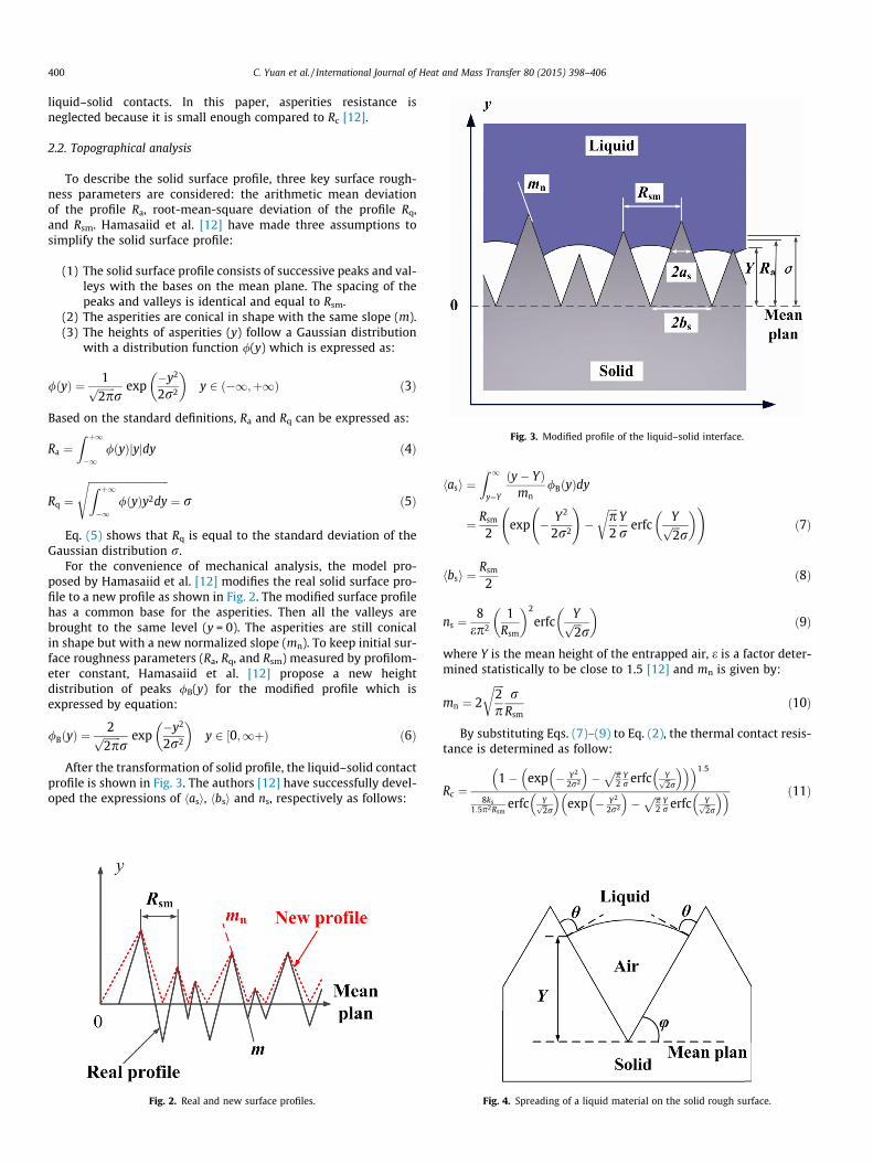
Fig. 3. Modified profile of the liquid–solid interface.

400 C. Yuan et al. / International Journal of Heat and Mass Transfer 80 (2015) 398–406

liquid–solid contacts. In this paper, asperities resistance isneglected because it is small enough compared to Rc [12].

2.2. Topographical analysis

To describe the solid surface profile, three key surface rough-ness parameters are considered: the arithmetic mean deviationof the profile Ra, root-mean-square deviation of the profile Rq,and Rsm. Hamasaiid et al. [12] have made three assumptions tosimplify the solid surface profile:

(1) The solid surface profile consists of successive peaks and val-leys with the bases on the mean plane. The spacing of thepeaks and valleys is identical and equal to Rsm.

(2) The asperities are conical in shape with the same slope (m).(3) The heights of asperities (y) follow a Gaussian distribution

with a distribution function /(y) which is expressed as:

/ðyÞ ¼ 1ffiffiffiffiffiffiffi2pp

rexp

�y2

2r2

� �y 2 �1;þ1ð Þ ð3Þ

Based on the standard definitions, Ra and Rq can be expressed as:

Ra ¼Z þ1

�1/ðyÞjyjdy ð4Þ

Rq ¼

ffiffiffiffiffiffiffiffiffiffiffiffiffiffiffiffiffiffiffiffiffiffiffiffiffiffiffiffiffiffiffiZ þ1

�1/ðyÞy2dy

s¼ r ð5Þ

Eq. (5) shows that Rq is equal to the standard deviation of theGaussian distribution r.

For the convenience of mechanical analysis, the model pro-posed by Hamasaiid et al. [12] modifies the real solid surface pro-file to a new profile as shown in Fig. 2. The modified surface profilehas a common base for the asperities. Then all the valleys arebrought to the same level (y = 0). The asperities are still conicalin shape but with a new normalized slope (mn). To keep initial sur-face roughness parameters (Ra, Rq, and Rsm) measured by profilom-eter constant, Hamasaiid et al. [12] propose a new heightdistribution of peaks /B(y) for the modified profile which isexpressed by equation:

/BðyÞ ¼2ffiffiffiffiffiffiffi

2pp

rexp

�y2

2r2

� �y 2 ½0;1þÞ ð6Þ

After the transformation of solid profile, the liquid–solid contactprofile is shown in Fig. 3. The authors [12] have successfully devel-oped the expressions of hasi, hbsi and ns, respectively as follows:

Fig. 2. Real and new surface profiles.

hasi ¼Z 1

y¼Y

ðy� YÞmn

/BðyÞdy

¼ Rsm

2exp � Y2

2r2

!�

ffiffiffiffip2

rYr

erfcYffiffiffi2p

r

� � !ð7Þ

hbsi ¼Rsm

2ð8Þ

ns ¼8

ep2

1Rsm

� �2

erfcYffiffiffi2p

r

� �ð9Þ

where Y is the mean height of the entrapped air, e is a factor deter-mined statistically to be close to 1.5 [12] and mn is given by:

mn ¼ 2

ffiffiffiffi2p

rr

Rsmð10Þ

By substituting Eqs. (7)–(9) to Eq. (2), the thermal contact resis-tance is determined as follow:

Rc ¼1� exp � Y2

2r2

� ��

ffiffiffip2

pYr erfc Yffiffi

2p

r

� �� �� �1:5

8ks1:5p2Rsm

erfc Yffiffi2p

r

� �exp � Y2

2r2

� ��

ffiffiffip2

pYr erfc Yffiffi

2p

r

� �� � ð11Þ

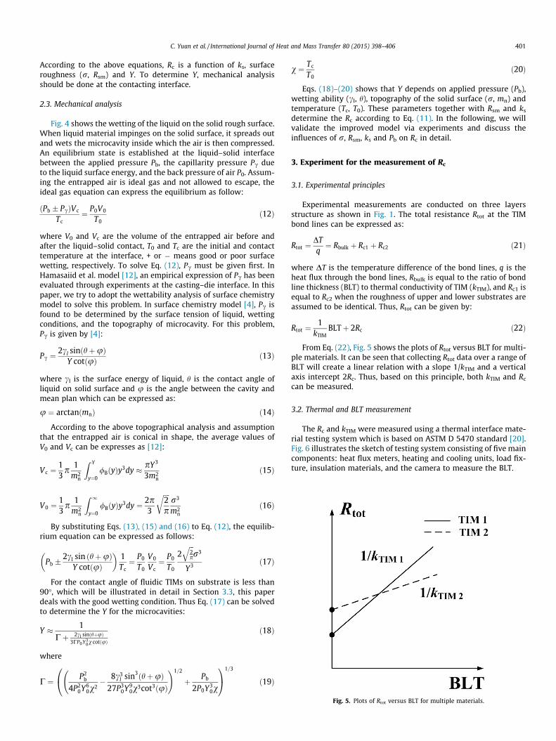
Fig. 4. Spreading of a liquid material on the solid rough surface.

C. Yuan et al. / International Journal of Heat and Mass Transfer 80 (2015) 398–406 401

According to the above equations, Rc is a function of ks, surfaceroughness (r, Rsm) and Y. To determine Y, mechanical analysisshould be done at the contacting interface.

2.3. Mechanical analysis

Fig. 4 shows the wetting of the liquid on the solid rough surface.When liquid material impinges on the solid surface, it spreads outand wets the microcavity inside which the air is then compressed.An equilibrium state is established at the liquid–solid interfacebetween the applied pressure Pb, the capillarity pressure Pc dueto the liquid surface energy, and the back pressure of air P0. Assum-ing the entrapped air is ideal gas and not allowed to escape, theideal gas equation can express the equilibrium as follow:

ðPb � PcÞVc

Tc¼ P0V0

T0ð12Þ

where V0 and Vc are the volume of the entrapped air before andafter the liquid–solid contact, T0 and Tc are the initial and contacttemperature at the interface, + or � means good or poor surfacewetting, respectively. To solve Eq. (12), Pc must be given first. InHamasaiid et al. model [12], an empirical expression of Pc has beenevaluated through experiments at the casting–die interface. In thispaper, we try to adopt the wettability analysis of surface chemistrymodel to solve this problem. In surface chemistry model [4], Pc isfound to be determined by the surface tension of liquid, wettingconditions, and the topography of microcavity. For this problem,Pc is given by [4]:

Pc ¼2cl sinðhþuÞ

Y cotðuÞ ð13Þ

where cl is the surface energy of liquid, h is the contact angle ofliquid on solid surface and u is the angle between the cavity andmean plan which can be expressed as:

u ¼ arctanðmnÞ ð14Þ

According to the above topographical analysis and assumptionthat the entrapped air is conical in shape, the average values ofV0 and Vc can be expresses as [12]:

V c ¼13p 1

m2n

Z Y

y¼0/BðyÞy3dy � pY3

3m2n

ð15Þ

V0 ¼13p 1

m2n

Z 1

y¼0/BðyÞy3dy ¼ 2p

3

ffiffiffiffi2p

rr3

m2n

ð16Þ

By substituting Eqs. (13), (15) and (16) to Eq. (12), the equilib-rium equation can be expressed as follows:

Pb �2cl sin hþuð Þ

Y cotðuÞ

� �1Tc¼ P0

T0

V0

Vc¼ P0

T0

2ffiffiffi2p

qr3

Y3 ð17Þ

For the contact angle of fluidic TIMs on substrate is less than90�, which will be illustrated in detail in Section 3.3, this paperdeals with the good wetting condition. Thus Eq. (17) can be solvedto determine the Y for the microcavities:

Y � 1

Cþ 2cl sinðhþuÞ3CP0Y3

0v cotðuÞ

ð18Þ

where

C ¼ P2b

4P20Y6

0v2� 8c3

l sin3ðhþuÞ27P3

0Y90v3cot3ðuÞ

!1=2

þ Pb

2P0Y30v

0@

1A

1=3

ð19Þ

v ¼ Tc

T0ð20Þ

Eqs. (18)–(20) shows that Y depends on applied pressure (Pb),wetting ability (cl, h), topography of the solid surface (r, mn) andtemperature (Tc, T0). These parameters together with Rsm and ks

determine the Rc according to Eq. (11). In the following, we willvalidate the improved model via experiments and discuss theinfluences of r, Rsm, ks and Pb on Rc in detail.

3. Experiment for the measurement of Rc

3.1. Experimental principles

Experimental measurements are conducted on three layersstructure as shown in Fig. 1. The total resistance Rtot at the TIMbond lines can be expressed as:

Rtot ¼DTq¼ Rbulk þ Rc1 þ Rc2 ð21Þ

where DT is the temperature difference of the bond lines, q is theheat flux through the bond lines, Rbulk is equal to the ratio of bondline thickness (BLT) to thermal conductivity of TIM (kTIM), and Rc1 isequal to Rc2 when the roughness of upper and lower substrates areassumed to be identical. Thus, Rtot can be given by:

Rtot ¼1

kTIMBLTþ 2Rc ð22Þ

From Eq. (22), Fig. 5 shows the plots of Rtot versus BLT for multi-ple materials. It can be seen that collecting Rtot data over a range ofBLT will create a linear relation with a slope 1/kTIM and a verticalaxis intercept 2Rc. Thus, based on this principle, both kTIM and Rc

can be measured.

3.2. Thermal and BLT measurement

The Rc and kTIM were measured using a thermal interface mate-rial testing system which is based on ASTM D 5470 standard [20].Fig. 6 illustrates the sketch of testing system consisting of five maincomponents: heat flux meters, heating and cooling units, load fix-ture, insulation materials, and the camera to measure the BLT.

Fig. 5. Plots of Rtot versus BLT for multiple materials.

Fig. 6. Sketch of the testing system.

Fig. 7. Use of shims to control BLT.

402 C. Yuan et al. / International Journal of Heat and Mass Transfer 80 (2015) 398–406

Heat flow through the specimen is measured by the heat fluxmeters with a 30 mm � 30 mm cross sectional area. It is accom-plished by measuring the linear temperature gradient dT/dx inthe heat flux meters and using the Fourier’s law of heat conductionq = k(dT/dx). The centerline temperature is measured at 10 mmintervals along each of the flux meter using five 1.5 mm diameterplatinum resistance temperature detectors (RTDs).

Power is applied by a heater block embedded with four wirewound cartridge heaters capable of 120 W. A water-cooled heatsink is designed to remove the heat rejected from the upper heatflux meter. The design uses a micro-pump with a maximum flowrate 2.3 � 10�5 m3/s to circulate water. Consequently heat flow influx meter is assured to be one-dimensional. The contact pressureon the specimen is controlled by the lead screws. A load cell with aresolution 3.3 kPa continuously monitors the applied load.

Insulation tapes with a thermal conductivity of 0.034 W m�1

K�1 and a thickness of 6 mm is placed around four sides of the heatflux meters to ensure the heat flow through the lower and uppermeters varies by less than 5%. 10 mm thick firebond insulation isplaced around four sides of heat block to eliminate heat leakageto the environment. Heat loss from the bottom is minimized byattaching it to 10 mm thick FR-4 epoxy material.

A camera with a microscope lens is implemented to measureBLT, as well as to detect the parallelism of the interface beforethe start of each test. Two 1 mm � 1 mm square marks areattached to the upper and lower flux meters located approximately2 mm from the flux meters edges. These marks are used as targetsand the camera measures the distance between the centers of thetargets. These marks are scanned in an approximately 5 mm fieldof view. The camera provides 1024 � 1024 bit resolution and eachpixel is approximately 5 lm in length, so the resolution of BLTmeasurement is limited to 5 lm. There are two steps to measureBLT. The first step is to apply a 1 MPa load between the heat fluxmeters without TIM and measure the targets distance L0. The sec-ond step is to separate the flux meters, fill the TIM between theflux meters and measure the targets distance L1 at the desired pres-sure. Then BLT is calculated by subtracting the L0 from L1.

For the measurement of Rc and kTIM, BLT of TIMs needs to becontrolled so that Rtot can be measured for a range of BLT as men-tioned above. In this experiment, stainless steel shims are mixed

into the TIMs to control the thickness as shown in Fig. 7. The shimsare 1.5 mm in diameter, and the thermal conduction through themis negligible which has been verified by Prasher et al. [21].Although the pressure from lead screws is applied on the sample,the shims take most of the pressure.

3.3. Sample preparation

Aluminium-6061 T4 blocks were chosen as the solid substrates,as well as the heat flux meters. The thermal conductivity is154 W m�1 K�1. Four couples of blocks were machined with differ-ent surface roughness. For each couple, surface roughness param-eters are measured by a Mitutoyo SJ-401 surface profilometer for12 times, and we set the average value as the roughness of the cou-ple. Shin Etsu KF96H silicone oil and Dow Corning TC5121 ther-mally conductive grease are prepared for the TIMs. Because thisexperiment can measure the thermal conductivity, the average val-ues of experimental results are set to be their thermal conductivi-ties. Eight experimental combinations of substrates roughness andTIMs are shown in Table 1.

The surface energy of the silicone oil was provided by the sup-plier, and that of the grease and aluminium substrate is measuredwith standard two liquid method using water and diiodomethane(CH2I2) based on the ASTM D 7490 standard [22]. This method canmeasure the polar and dispersion components of the material sur-face energy, cp and cd, respectively. The total surface energy of thematerial is the sum of cp and cd. The contact angle of silicone oilwas directly measured on the smoothest aluminium substrate bysessile drop method [23]. However, because thermal grease hasextremely high viscosity, the method cannot be used for grease.The contact angle of grease on the aluminium substrate can be cal-culated by using the equation [23]:

ð1þ cos hÞcl ¼ 2ffiffiffiffiffiffiffiffiffiffiffiffiffiffiffiffiffiffiffiffiffiffiffiffiffiffiffiffiffifficlpcsp þ cldcsd

pð23Þ

where the subscripts l and s refer to the liquid and substrate,respectively. Because cp and cd of the grease and substrate havebeen measured, the contact angle can be calculated. Table 2 showsthe surface energy of silicone oil, thermal grease, and aluminiumblock, and the contact angle of silicone oil and thermal grease onthe aluminium block.

Table 1Experimental combinations for the measurement of Rc.

Materials Silicone oil (kTIM 1) Grease (kTIM 2)

Aluminium 154 W m�1 K�1 r = 0.23 lm Rsm = 99.2 lm 1 5r = 0.34 lm Rsm = 90.8 lm 2 6r = 0.72 lm Rsm = 132.1 lm 3 7r = 1.13 lm Rsm = 166.4 lm 4 8

Table 2Surface energy of TIMs and aluminium block, and the contact angle of TIMs on theblock.

Silicone oil Thermal grease Aluminium block

cp (mN m�1) – 24.2 41.6cd (mN m�1) – 14.0 4.2c (mN m�1) 21.3 38.2 45.8h (deg) 22.3 45.0 –

Fig. 8. (a) Plots of thermal resistance R versus BLT; (b) Comparison of the modelresults with experimental data for silicone oil.

Fig. 9. (a) Plots of thermal resistance R versus BLT; (b) Comparison of the modelresults with experimental data for thermal grease.

Table 3Linear regression equations and correlation coefficients of all groups.

Group Linear regression equations Correlation coefficients r2

1 R = 4.64 � BLT + 1.431 � 10�4 0.99702 R = 4.57 � BLT + 1.217 � 10�4 0.98993 R = 4.49 � BLT + 2.140 � 10�4 0.99494 R = 6.02 � BLT + 3.003 � 10�4 0.98725 R = 0.383 � BLT + 1.299 � 10�5 0.99116 R = 0.373 � BLT + 1.175 � 10�5 0.98567 R = 0.465 � BLT + 1.898 � 10�5 0.99528 R = 0.431 � BLT + 3.369 � 10�5 0.9991

C. Yuan et al. / International Journal of Heat and Mass Transfer 80 (2015) 398–406 403

3.4. Error analysis

According to Eq. (22), the error in Rc is given as [24]

DRc

Rc¼ �

ffiffiffiffiffiffiffiffiffiffiffiffiffiffiffiffiffiffiffiffiffiffiffiffiffiffiffiffiffiffiffiffiffiffiffiffiffiffiffiffiffiffiffiffiffiffiffiffiffiffiffiffiffiffiffiffiffiffiffiffiffiffiffiffiffiffiffiffiffiffiffiffiffiffiffiffiffiffiffiffiffiffiffiffiffiffiffiffiffiffiffiffiffiffiffiffiffiffiffiffiffiffiffiffiffiffiffiffiffiffiffiffiffiffiffiDR

Rtot � BLT=kTIMð Þ=2

� �2

þ 1

k2TIM

DBLTðRtot � BLT=kTIMÞ=2

� �2vuut

ð24Þ

Following the method in Ref. [25], the errors in R for the siliconeoil and grease are measured with 3.8 � 10�6 m2 K W�1 and1.3 � 10�6 m2 K W�1, respectively. The error in BLT is 5 lm whichis equal to the pixel size of the camera.

4. Validation and discussion

4.1. Comparison of experimental data with the model

For the all experimental combinations, experiments were con-ducted for four different BLTs to find out Rc and kTIM. Figs. 8 and9(a) show the plots of thermal resistance R versus BLT for the sili-cone oil and thermal grease, respectively. It is shown that R is lin-early dependent on BLT, thus Rc and kTIM can be computed by thelinear least square method. The solved linear regression equationsand correlation coefficients are given in Table 3. According to

Fig. 10. (a) Scatters of thermal resistance R versus BLT for the group 7 withdifference applied pressures; (b) Comparison of the model results with experimen-tal data.

Fig. 12. Variation of hasi/hbsi and hasi � ns with (a) r when Rsm keeps constant; (b)Rsm when r keeps constant.

404 C. Yuan et al. / International Journal of Heat and Mass Transfer 80 (2015) 398–406

Eq. (22), thermal conductivity of silicone oil can be obtained bytaking the average of the 1/slope of the groups 1 to 4 linear equa-tions, which is equal to 0.21 W m�1 K�1. In the same way, thermalconductivity of grease can be computed, which is equal to2.44 W m�1 K�1. Meanwhile, Rc for each group can be obtainedby taking half of the intercept of the linear regression equations.Figs. 8 and 9(b) show the experimental results of Rc for the siliconeoil and thermal grease, respectively, as well as the error bars.According to Eq. (24), the biases of silicone oil and grease fromthe experiments are 2.41 � 10�5 m2 K W�1 and 2.43 � 10�6

m2 K W�1, respectively.As mentioned above, predicting Rc needs to obtain the parame-

ters as follow: topography parameters (r, Rsm), wettability param-eters (cl, h), mechanical parameter (Pb), and thermal parameters

Fig. 11. Variation of Rc with r and Rsm respectively when one of them keepsconstant.

(ks, T0, Tc). In the experiments of groups 1 to 8, Pb is 0.1 MPa, T0

is 288 K, and Tc is approximately 323 K by taking the average tem-perature of the TIMs in the testing. Other parameters can beobtained in Tables 1 and 2. Figs. 8 and 9(b) show the model resultsof Rc for all groups. Compared with the experimental results, it canbe found that the improved model matches well with experimentaldata. The deviation between the experimental and model results isless than 14.3%.

In order to study the influence of Pb on Rc, different pressuresvaried from 0.13 MPa to 0.48 MPa were set on group 7 withoutthe shims controlling the BLT. Fig. 10(a) shows the scatters of

Fig. 13. Variation of Y as a function Pb.

Fig. 14. (a) Variation of Rc and (b) Pc/P0 with cl when h keeps constant.

Fig. 15. (a) Variation of Rc and (b) Pc/P0 with h when cl keeps constant.

C. Yuan et al. / International Journal of Heat and Mass Transfer 80 (2015) 398–406 405

measured R versus measured BLTs. Based on Eq. (22), the values ofRc with various pressures can be computed. Fig. 10(b) shows thecomparison between the experimental and model results. At lowerpressure, the model matches well with experimental results. Butthe model predictions tend to deviate at higher pressure owingto the higher relative error in thin BLT measurement.

4.2. Influence of the parameters on the model results

In the Ref. [12], the authors have highlighted the effect of sur-face roughness on Rc in liquid–solid interface. According to theirpredictive model, r does not have any influence on Rc, while Rsm

has more effect on Rc. Similar results can be found in the improvedmodel. Using the parameters of group 7, Fig. 11 respectively pre-sents the curves of Rc versus r and Rsm when one of them keepsconstant. It is shown that Rc changes hardly with r, but increaseswith Rsm obviously. In order to explain the results, Fig. 12 showsthe plots of hasi/hbsi and hasi � ns as a functions of r and those asa functions of Rsm. When Rsm keeps constant, r nearly has no sig-nificant influence on hasi/hbsi or hasi � ns. Thus Rc does not changewith r according to Eq. (2). Contrary to r, the larger the value ofRsm, the smaller the hasi � ns. And the hasi/hbsi still remains con-stant so that Rc turns larger according to Eq. (2). Comparing theRc between groups 1 and 2 in Fig. 8(b), or between groups 5 and6 in Fig. 9(b), the experimental results seem to be accorded withthe claim that Rsm has the more important impact on Rc. However,the considerable experimental bias and the limited experimentalsamples fail to make it credible enough to verify the point. Thusit is desired to investigate this work in the future to validate theresults of the improved Rc model.

Comparing the predictive results of Rc between the groups hav-ing the same roughness parameters, such as groups 1 and 5, groups2 and 6, and so on, it can be found that Rc is approximately inver-sely proportional to thermal conductivity of TIMs. Thermal con-ductivity of aluminium is much larger than kTIM and this makesks approximately equal to 2kTIM. Then Eq. (2) shows Rc varies inan inverse proportion to kTIM.

As illustrated in Fig. 10(b), Rc decreases with Pb increasing. Tobetter understand the effect of Pb on Rc, Y is plotted as a functionof Pb and it is shown in Fig. 13. It shows that Y decreases with Pb

increasing. Thus higher Pb makes the liquid and solid contact betterand result in a lower Rc at the interface.

Finally, the effect of wettability parameters (cl, h) on Rc is inves-tigated. Figs. 14 and 15(a) respectively presents the curves of Rc

versus cl and h for the groups 5–8. From Fig. 14(a), it is seen thatRc tendentially decreases with cl increasing when h is equal to45.0�. Fig. 14(b) plots Pc/P0 as a function of cl. The figure shows thatPc increases with cl increasing. Then Y decreases according to Eq.(18) and finally Rc decreases. From the figure, it can be also foundthat the larger Rsm is, the lower Pc is. On the other hand, Fig. 15(a)shows a very slow decrease of Rc with h increasing when cl is rel-atively small and equal to 38.2 mN m�1. In order to explain theresults, Pc/P0 is plotted as a function of h as shown in Fig. 15(b).It shows that Pc increase with h increasing. However the value ofPc is much smaller than P0 which means Pc makes less contributionto Y. So for the materials with small cl, Rc hardly changes with h.

5. Conclusion

This paper proposes an improved model for predicting thermalcontact resistance Rc at the liquid–solid interface based on Hamas-aiid et al. model. Through conducting the wettability analysis onthe liquid–solid contact, an explicit expression is derived to predictthe height of entrapped air between the liquid and solid. Experi-mental measurements have been conducted on TIMs-aluminium

406 C. Yuan et al. / International Journal of Heat and Mass Transfer 80 (2015) 398–406

interface. The results show the model matches well with the exper-imental data.

The proposed model shows that compared to standard devia-tion of the asperities heights r, the mean asperity peak spacingRsm has more effect on Rc, and Rc decreases with Rsm. It is observedthat Rc varies with thermal conductivity of TIMs kTIM in an inverseproportion, when the thermal conductivity of solid substrate ismuch larger than kTIM. The extrapolation of the height of theentrapped air Y has shown that it is directly dependent on appliedpressure Pb. Higher Pb can make liquid and solid contact better andresults in a lower Rc. Rc tendentially decreases with surface energyof liquid cl. For the materials with small cl, Rc hardly changes withcontact angle of liquid on solid surface h.

Conflict of interest

None declared.

Acknowledgements

The authors would like to acknowledge the financial supportpartly by National Science Foundation of China (51376070), andpartly by 973 Project of The Ministry of Science and Technologyof China (2011CB013105).

References

[1] R.S. Prasher, J. Shipley, S. Prstic, P. Koning, J.L. Wang, Thermal resistance ofparticle laden polymeric thermal interface materials, J. Heat Transfer 125 (6)(2003) 1170–1177.

[2] R.S. Prasher, Rheology based modeling and design of particle laden polymericthermal interface materials, IEEE Trans. Compon. Packag. T. 28 (2) (2005) 230–237.

[3] R.S. Prasher, Thermal interface materials: historical perspective, status, andfuture directions, Proc. IEEE 94 (8) (2006) 1571–1586.

[4] R.S. Prasher, Surface chemistry and characteristic based model for the thermalcontact resistance of fluidic interstitial thermal interface materials, J. HeatTransfer 123 (5) (2001) 969–975.

[5] C.R. Tien, A correlation for thermal contact conductance of nominally-flatsurfaces in vacuum, in: Proc. 7th Thermal Conductivity Conference, U. S.Bureau of Standards, 1968, pp. 755–759.

[6] M.G. Cooper, B.B. Mikic, M.M. Yovanovich, Thermal contact conductance, Int. J.Heat Mass Transfer 12 (3) (1969) 279–300.

[7] T.R. Thomas, S.D. Probert, Thermal contact resistance: the directional effectand other problems, Int. J. Heat Mass Transfer 13 (5) (1970) 789–807.

[8] B.B. Mikic, Thermal contact conductance: theoretical considerations, Int. J.Heat Mass Transfer 17 (2) (1974) 205–214.

[9] T. Bennett, P. Poulikakos, Heat transfer aspects of splat-quench solidification:modelling and experiment, J. Mater. Sci. 29 (8) (1994) 2025–2039.

[10] W. Liu, G.X. Wang, E.F. Matthys, Thermal analysis and measurements for amolten metal drop impacting on a substrate: cooling, solidification and heattransfer coefficient, Int. J. Heat Mass Transfer 38 (8) (1995) 1387–1395.

[11] A. Hamasaiid, G. Dour, T. Loulou, M. Dargusch, A predictive model for theevolution of the thermal conductance at the casting-die interfaces in highpressure die casting, Int. J. Therm. Sci. 49 (2) (2010) 365–372.

[12] A. Hamasaiid, M. Dargusch, T. Loulou, G. Dour, A predictive model for thethermal contact resistance at liquid–solid interfaces: analytical developmentsand validation, Int. J. Therm. Sci. 50 (8) (2011) 1445–1459.

[13] C.V. Madhusudana, Thermal Contact Conductance, Springer-Verlag, New York,1996.

[14] SJ-401 Surface Roughness Tester User’s Manual, Mitutoyo Corporation, Japan.[15] M.R. Sridhar, M.M. Yovanovich, Review of elastic and plastic contact

conductance models: comparison with experiment, J. Thermophys. HeatTransfer 8 (4) (1994) 633–640.

[16] M.R. Sridhar, M.M. Yovanovich, Elastoplastic contact conductance model forisotropic conforming rough surfaces and comparison with experiments, J.Thermophys. Heat Transfer 118 (1) (1996) 3–9.

[17] M. Bahrami, M.M. Yovanovich, J.R. Culham, Thermal joint resistances ofnonconforming rough surfaces with gas-filled gaps, J. Thermophys. HeatTransfer 18 (3) (2004) 326–332.

[18] M. Bahrami, J.R. Culham, M.M. Yovanovich, G.E. Schneider, Thermal contactresistance of nonconforming rough surfaces, part 1: contact mechanics model,J. Thermophys. Heat Transfer 18 (2) (2004) 209–217.

[19] M. Bahrami, J.R. Culham, M.M. Yovanovich, G.E. Schneider, Thermal contactresistance of nonconforming rough surfaces, part 2: thermal model, J.Thermophys. Heat Transfer 18 (2) (2004) 218–227.

[20] ASTM Standard D-5470-06, Standard test method for thermal transmissionproperties of thermally conductive electrical insulation materials, CopyrightASTM International, Conshohocken, PA, 2007.

[21] R.S. Prasher, P. Koning, J. Shipley, A. Devpura, Dependence of thermalconductivity and mechanical rigidity of particle-laden polymeric thermalinterface material on particle volume fraction, J. Electron. Packag. 125 (3)(2003) 386–391.

[22] ASTM Standard D-7490-13, Standard test method for measurement ofthe surface tension of solid coatings, substrates and pigments usingcontact angle measurements, Copyright ASTM International, Conshohocken,PA, 2013.

[23] S. Wu, Polymer Interface and Adhesion, Marcel Dekker, New York, 1982.[24] S.J. Kline, F.A. McClintock, Describing uncertainties in single sample

experiments, Mech. Eng. 75 (1953) 3–8.[25] R.S. Prasher, C. Simmons, G. Solbrekken, Thermal contact resistance of phase

change and grease type polymeric materials, in: Proceedings of InternationalMechanical Engineering Congress and Exposition, Orlando, Florida, 2000.