© 2005 International Monetary Fund July 2005 IMF Country Report No. 05/225

Kingdom of the Netherlands––Netherlands: Selected Issues This Selected Issues paper for the Kingdom of the Netherlands––Netherlands was prepared by a staff team of the International Monetary Fund as background documentation for the periodic consultation with the member country. It is based on the information available at the time it was completed on June 6, 2005. The views expressed in this document are those of the staff team and do not necessarily reflect the views of the government of the Kingdom of the Netherlands––Netherlands or the Executive Board of the IMF. The policy of publication of staff reports and other documents by the IMF allows for the deletion of market-sensitive information.

To assist the IMF in evaluating the publication policy, reader comments are invited and may be sent by e-mail to Publicationpolicy@imf.org.

Copies of this report are available to the public from International Monetary Fund ● Publication Services 700 19th Street, N.W. ● Washington, D.C. 20431

Telephone: (202) 623 7430 ● Telefax: (202) 623 7201 E-mail: publications@imf.org ● Internet: http://www.imf.org

Price: $15.00 a copy

International Monetary Fund

Washington, D.C.

INTERNATIONAL MONETARY FUND

KINGDOM OF THE NETHERLANDS—NETHERLANDS

Selected Issues

Prepared by David Hofman and Francisco Nadal De Simone (both EUR) and Mark Walsh (ICM)

Approved by the European Department

June 6, 2005

Contents Page

I. The External Competitiveness of the Dutch Economy: A Short Note on Evidence from both Aggregate and Disaggregate Data..................................................3 A. Overview....................................................................................................................3 B. Recent Developments in Competitiveness.................................................................3 C. Aggregate Trade Data ................................................................................................5 II. Long-Run Household Consumption Equilibrium in the Netherlands................................9 A. Overview and Introduction ........................................................................................9 B. The Standard Consumption Model ..........................................................................10 C. Data and Data Issues................................................................................................11 D. The Long-Run Elasticities of the Model..................................................................12 E. Concluding Remarks................................................................................................14 References................................................................................................................................16 III. House Prices in the Netherlands ......................................................................................25 A. Introduction..............................................................................................................25 B. Brief Review of the Literature .................................................................................26 C. The Conceptual Framework.....................................................................................28 D. The Data...................................................................................................................29 E. Econometric Issues and Hypothesis Tests ...............................................................30 F. Empirical Results .....................................................................................................31 G. Concluding Remarks................................................................................................32 References................................................................................................................................33 IV. Budgetary Policymaking in the Netherlands ...................................................................42 A. Introduction..............................................................................................................42 B. Fiscal Policy Before 1994........................................................................................43 C. Medium-Term Expenditure Framework ..................................................................43 D. Role of the CPB .......................................................................................................50

- 2 -

E. Performance Budgeting ...........................................................................................53 F. Summary and Conclusions ......................................................................................54 References................................................................................................................................56 V. The Financial Sector in the Netherlands: A Health Check and Progress Report on the FSSA Recommendations ...................................................................................57 A. Recent Developments ..............................................................................................57 B. FSSA Recommendations .........................................................................................60 Figures I.1 Real Exchange Rate .......................................................................................................4 I.2 Dutch Export Share in World Market............................................................................6 II.1 Consumption, Income, and Net Worth ........................................................................19 II.2 Unemployment Rate ....................................................................................................19 II.3 Interest Rates and Stock Market Returns.....................................................................20 II.4 Stock Market Price Index.............................................................................................20 II.5 Real House Prices ........................................................................................................21 II.6 Real Household Net Worth/Income.............................................................................21 II.7 Consumption and Estimated Long-Run Consumption ................................................22 III.1 Ratio of House Prices over Disposable Income 1970:Q1–2004:Q2............................35 III.2 Price-Rent Ratio, 1970:Q1–2004:Q2...........................................................................35 III.3 Real House Prices, 1970:Q1–2004:Q2 ........................................................................36 III.4 Household Disposable Income and Mortgage Rates, 1970:Q1–2004:Q2 ...................37 III.5 Actual House Prices Versus Their Long-Run Equilibrium, 1970:Q1–2004:Q2 .........38 IV.1 Expenditure Development, 1999–2003 .......................................................................46 IV.2 Trends in Public Finances, 1970–2004........................................................................48 Tables I.1 Unit Labor Costs in the Netherlands and its Competitors .............................................4 I.2 Dutch Unit Labor Costs, Manufacturing, 2001–06 .......................................................5 I.3 CMS Analysis of Exports Changes................................................................................8 II.1 Elliot, Rothenberg, and Stock Test for Unit Roots ......................................................23 II.2 Johansen-Juselius Maximum Likelihood Test for Cointegration ................................24 III.1 Unit Root Tests ............................................................................................................39 III.2 Lag Order Selection Criteria........................................................................................39 III.3 Johansen Cointegration Test ........................................................................................40 III.4 Estimation Results .......................................................................................................41 V.1 Financial System Structure ..........................................................................................64 V.2 Encouraged Financial Soundness Indicators ...............................................................65 V.3 Financial Sector Indicators ..........................................................................................66 V.4 Performance of Dutch Pension Funds..........................................................................66 Appendix II.1 Detailed Econometric Results......................................................................................17

- 3 -

I. THE EXTERNAL COMPETITIVENESS OF THE DUTCH ECONOMY: A SHORT NOTE ON EVIDENCE FROM BOTH AGGREGATE AND DISAGGREGATE DATA1

A. Overview

1. Though the level of Dutch competitiveness remains high in absolute terms, concerns have arisen about its deterioration in recent years. The relatively poor economic performance during the new millennium contributed to these concerns generally, as did restrained export performance more specifically. Against this background, this note provides a brief analysis of the competitiveness of the Dutch economy. It assesses aggregate measures of competitiveness and shows that the recent worsening, though not particularly evident in the aggregate trade share data, does appear in the analysis of disaggregated trade share data.

B. Recent Developments in Competitiveness

2. While the Netherlands remains a highly competitive economy in absolute terms, it has undergone a marked decline in competitiveness in recent years. This is confirmed by both the World Economic Forum’s (WEF) and the International Institute for Management (IMD)’s recent international competitiveness rankings. These broad-based measures, which attempt to look beyond economic performance to consider economies’ official sectors, business efficiency, and infrastructure quality, have consistently ranked the Netherlands highly. In the WEF’s growth competitiveness index for 2004, when ranked against 103 other countries, the Netherlands was placed 12th, while under the IMD’s methodology, the Dutch economy ranks 13th out of 60 countries in the 2005 listing. However, these same rankings also serve to demonstrate the decline in competitiveness. For example, while the Netherlands was ranked 4th internationally in 2000 under the IMD’s methodology, the ranking declined to 13th in 2003 and 15th in 2004. These broad-based findings are confirmed by more traditional aggregate measures of competitiveness.

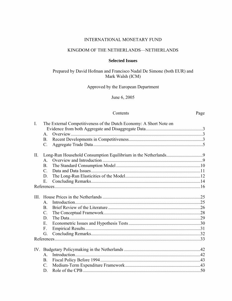
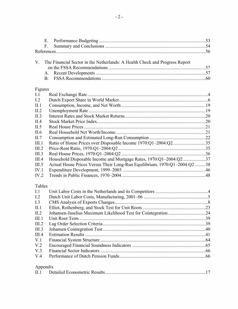
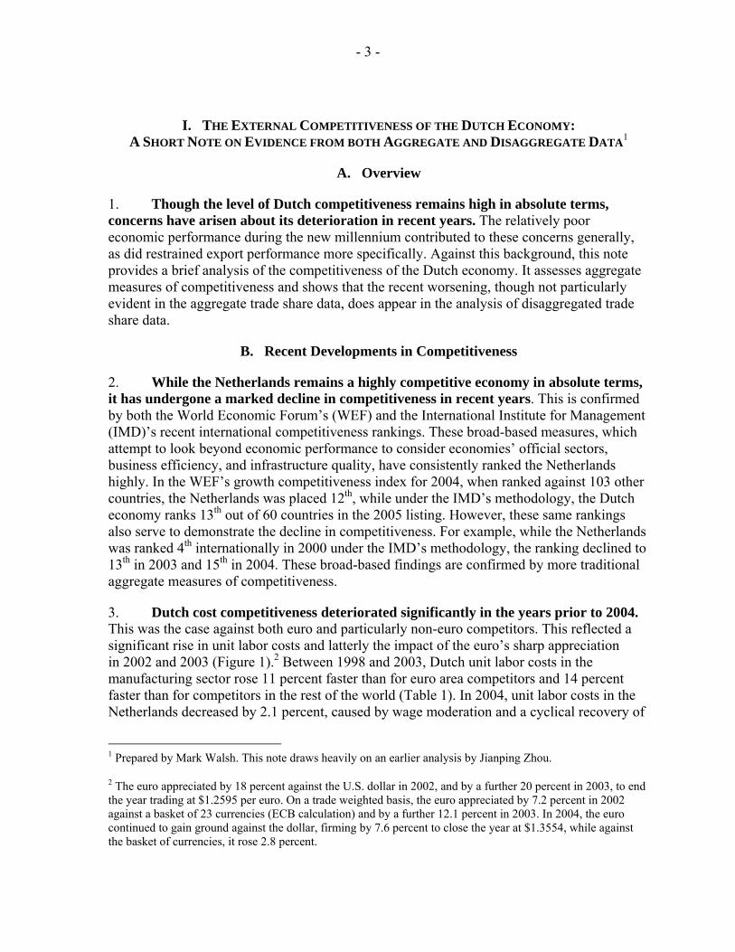
3. Dutch cost competitiveness deteriorated significantly in the years prior to 2004. This was the case against both euro and particularly non-euro competitors. This reflected a significant rise in unit labor costs and latterly the impact of the euro’s sharp appreciation in 2002 and 2003 (Figure 1).2 Between 1998 and 2003, Dutch unit labor costs in the manufacturing sector rose 11 percent faster than for euro area competitors and 14 percent faster than for competitors in the rest of the world (Table 1). In 2004, unit labor costs in the Netherlands decreased by 2.1 percent, caused by wage moderation and a cyclical recovery of

1 Prepared by Mark Walsh. This note draws heavily on an earlier analysis by Jianping Zhou.

2 The euro appreciated by 18 percent against the U.S. dollar in 2002, and by a further 20 percent in 2003, to end the year trading at $1.2595 per euro. On a trade weighted basis, the euro appreciated by 7.2 percent in 2002 against a basket of 23 currencies (ECB calculation) and by a further 12.1 percent in 2003. In 2004, the euro continued to gain ground against the dollar, firming by 7.6 percent to close the year at $1.3554, while against the basket of currencies, it rose 2.8 percent.

- 4 -

labor productivity growth. This ended seven consecutive years of worsening cost competitiveness against euro competitors. However, because of the ongoing euro appreciation, the deterioration of cost competitiveness against non-euro competitors continued (Table 2).

Figure 1. Netherlands: Real Exchange Rate

90

95

100

105

110

115

120

1990M1 1993M1 1996M1 1999M1 2002M1 2005M1

Real Effective Exchange Rate (NULC Based)Nominal Effective Exchange RateReal Effective Exchange Rate (CPI Based)

Netherlands Euro-zone Competitors Other Competitors

1998 1.9 -0.9 2.21999 0.8 0.8 3.62000 0.3 -1.0 12.62001 4.9 2.7 2.32002 4.3 1.9 -4.92003 3.5 1.3 -11.82004 -2.1 -2.0 -7.1

Sources: CPB; and ministry of finance.

Table 1. Netherlands: Unit Labor Costs in the Netherlands and its Competitors(Annual changes in percent)

- 5 -

2001 2002 2003 2004

The Netherlands

Compensation per employee 1/ 4.6 6.5 3.7 2.4Labor productivity -0.3 2.2 0.3 4.6Unit labor costs 4.9 4.3 3.5 -2.1

Euro competitors

Compensation per employee 1/ 3.3 4.0 3.2 2.4Labor productivity 0.6 2.1 1.9 4.4Unit labor costs 2.7 1.9 1.3 -2.0

Non-euro competitors

Compensation per employee 1/ 6.4 4.0 7.1 4.3Labor productivity 2.4 4.9 6.3 6.3Effective exchange rate (euro) 1.6 4.2 14.2 5.6Unit labor costs 2.3 -4.9 -11.8 -7.1

All competitors

Compensation per employee 1/ 4.9 4.0 5.6 3.4Labor productivity 1.5 3.6 4.1 5.4Effective exchange rate (euro) 0.8 2.2 7.5 3.0Unit labor costs 2.5 -1.7 -5.6 -4.7

Source: CPB.

1/ In local currency.

(Annual changes in percent)

Table 2. Netherlands: Dutch Unit Labor Costs, Manufacturing, 2001-06

4. Export performance, in volume terms, appears to have reflected the loss in competitiveness. Real export growth averaged less than 1 percent in 2001–03, at a time when the growth in the Dutch export market was averaging above 2 percent annually according to WEO data. Year-average real export growth (goods and services) in 2004 was about 8 percent, increasing roughly in line with market growth. However, much of the increase in exports in 2004 was driven by the sharp growth in re-exports.

C. Aggregate Trade Data

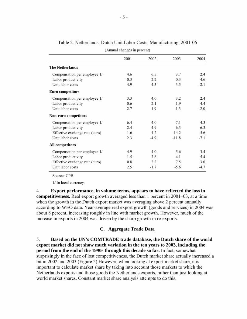
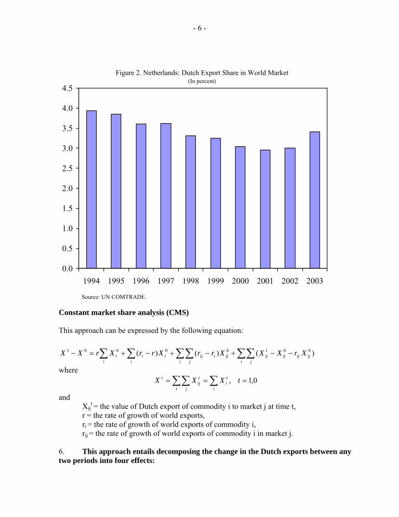
5. Based on the UN’s COMTRADE trade database, the Dutch share of the world export market did not show much variation in the ten years to 2003, including the period from the end of the 1990s through this decade so far. In fact, somewhat surprisingly in the face of lost competitiveness, the Dutch market share actually increased a bit in 2002 and 2003 (Figure 2).However, when looking at export market share, it is important to calculate market share by taking into account those markets to which the Netherlands exports and those goods the Netherlands exports, rather than just looking at world market shares. Constant market share analysis attempts to do this.

- 6 -

0.0

0.5

1.0

1.5

2.0

2.5

3.0

3.5

4.0

4.5

1994 1995 1996 1997 1998 1999 2000 2001 2002 2003

Source: UN COMTRADE.

Figure 2. Netherlands: Dutch Export Share in World Market(In percent)

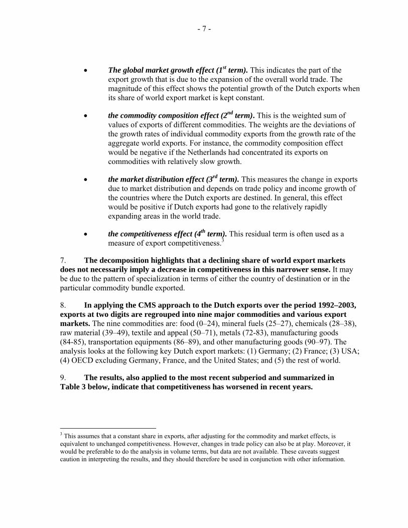
Constant market share analysis (CMS) This approach can be expressed by the following equation:

∑∑ ∑∑∑∑ −−+−+−+=−i j i j

ijijijijijiiji

iii

i XrXXXrrXrrXrXX )()()( 00100001

where ∑ ∑∑ ===

i i

ti

j

tij

t tXXX 0,1,

and Xij

t = the value of Dutch export of commodity i to market j at time t, r = the rate of growth of world exports, ri = the rate of growth of world exports of commodity i,

rij = the rate of growth of world exports of commodity i in market j. 6. This approach entails decomposing the change in the Dutch exports between any two periods into four effects:

- 7 -

• The global market growth effect (1st term). This indicates the part of the export growth that is due to the expansion of the overall world trade. The magnitude of this effect shows the potential growth of the Dutch exports when its share of world export market is kept constant.

• the commodity composition effect (2nd term). This is the weighted sum of values of exports of different commodities. The weights are the deviations of the growth rates of individual commodity exports from the growth rate of the aggregate world exports. For instance, the commodity composition effect would be negative if the Netherlands had concentrated its exports on commodities with relatively slow growth.

• the market distribution effect (3rd term). This measures the change in exports due to market distribution and depends on trade policy and income growth of the countries where the Dutch exports are destined. In general, this effect would be positive if Dutch exports had gone to the relatively rapidly expanding areas in the world trade.

• the competitiveness effect (4th term). This residual term is often used as a measure of export competitiveness.3

7. The decomposition highlights that a declining share of world export markets does not necessarily imply a decrease in competitiveness in this narrower sense. It may be due to the pattern of specialization in terms of either the country of destination or in the particular commodity bundle exported.

8. In applying the CMS approach to the Dutch exports over the period 1992–2003, exports at two digits are regrouped into nine major commodities and various export markets. The nine commodities are: food (0–24), mineral fuels (25–27), chemicals (28–38), raw material (39–49), textile and appeal (50–71), metals (72-83), manufacturing goods (84-85), transportation equipments (86–89), and other manufacturing goods (90–97). The analysis looks at the following key Dutch export markets: (1) Germany; (2) France; (3) USA; (4) OECD excluding Germany, France, and the United States; and (5) the rest of world.

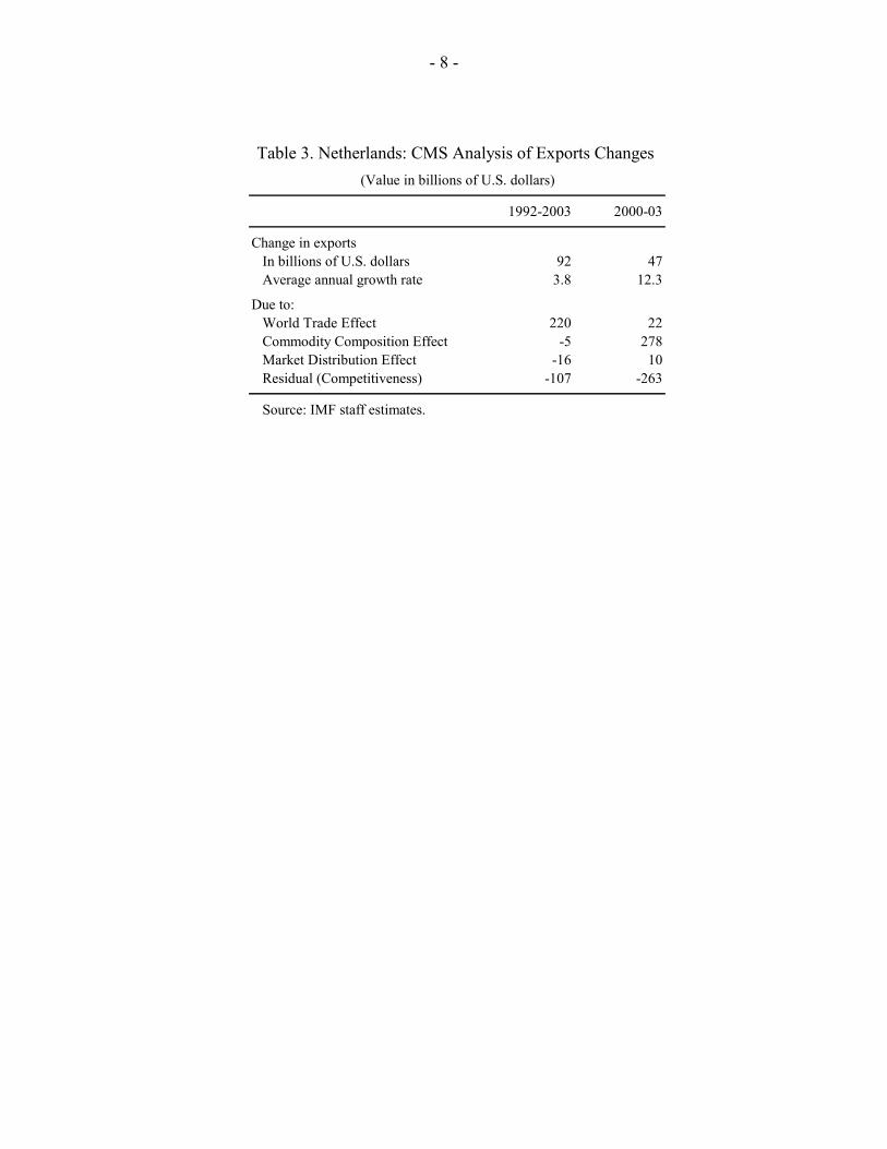
9. The results, also applied to the most recent subperiod and summarized in Table 3 below, indicate that competitiveness has worsened in recent years.

3 This assumes that a constant share in exports, after adjusting for the commodity and market effects, is equivalent to unchanged competitiveness. However, changes in trade policy can also be at play. Moreover, it would be preferable to do the analysis in volume terms, but data are not available. These caveats suggest caution in interpreting the results, and they should therefore be used in conjunction with other information.

- 8 -

1992-2003 2000-03

Change in exports In billions of U.S. dollars 92 47 Average annual growth rate 3.8 12.3

Due to:World Trade Effect 220 22Commodity Composition Effect -5 278Market Distribution Effect -16 10Residual (Competitiveness) -107 -263

Source: IMF staff estimates.

Table 3. Netherlands: CMS Analysis of Exports Changes (Value in billions of U.S. dollars)

- 9 -

II. LONG-RUN HOUSEHOLD CONSUMPTION EQUILIBRIUM IN THE NETHERLANDS4

A. Overview and Introduction

10. Private consumption growth in the Netherlands has been sluggish in recent years. Since the beginning of 2001, the average quarterly growth rate has been about ¼ percent as opposed to an average of nearly 1 percent in the second half of the 1990s. Given its share in final demand, changes in consumption have a large impact on GDP growth. This, as well as the disappointing growth performance so far this decade, explain why consumer behavior has moved to center stage in policy discussions.

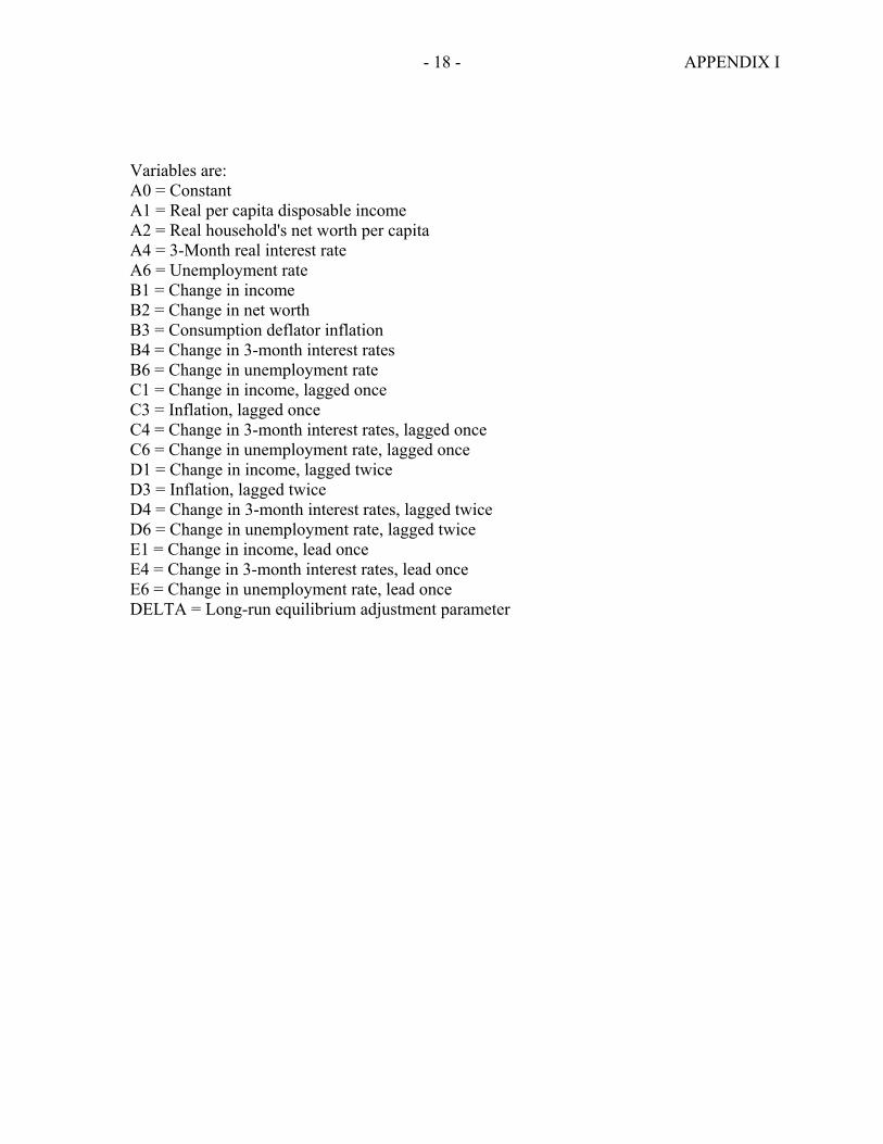
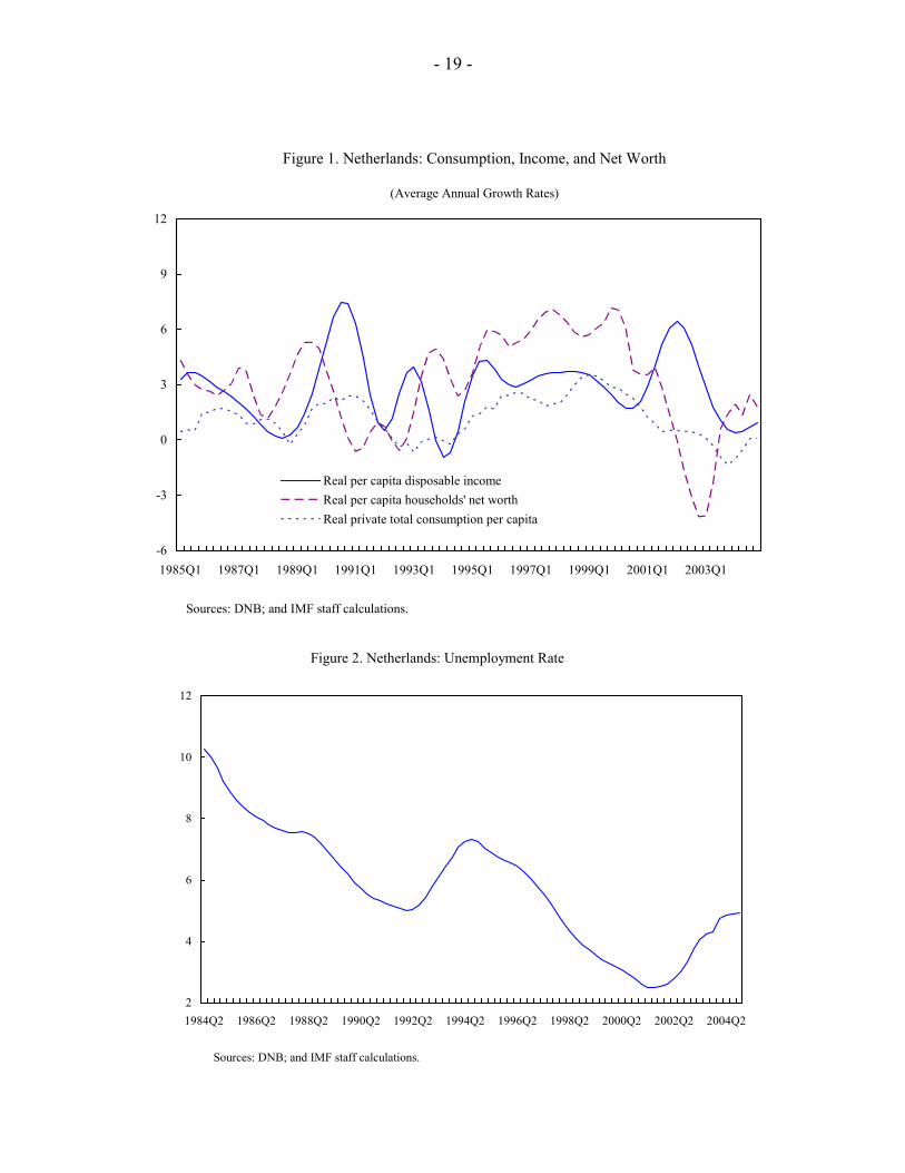
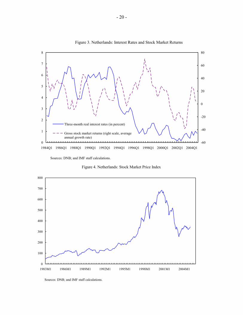
11. Recent consumption behavior cannot be explained by developments in disposable income alone. The deceleration of private consumption growth started earlier than the deceleration of per capita real disposable income growth, and occurred at a time when the unemployment rate was at a historic low and interest rates had declined (Figures 1 to 3). A key related observation is that the average share of disposable income in GDP fell by over 2 percentage points when comparing 2001–04 with 1995–2000. This largely reflected a decline in property income. Corresponding to this, Dutch consumers cut consumption and savings in relation to GDP in roughly equal amounts.5

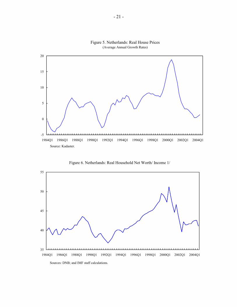
12. This background suggests looking at the role of wealth as an influence on private consumption behavior. In this connection, the Amsterdam stock exchange price index started to fall in the second quarter of 2001 (Figure 4). In addition, the ratio of per capita household net worth to income clearly started to decline toward end-2001, partly influenced by a slowing in the pace of house price increases (Figures 5 and 6). Consistent with historical evidence, consumer confidence rapidly deteriorated, more or less in tandem with the decline in stock prices (Jansen and Nahuis, 2003). The Dutch central bank has also associated the decline in consumer confidence to doubts about pension funds solvency, dissatisfaction with public services, and overall policy and political uncertainty (De Nederlandsche Bank, 2004).

13. This paper focuses on the long-run determinants of and short-term outlook for Dutch total private consumption. A cointegration model is estimated to test the relevance of a number of factors suggested by the literature on consumption behavior, such as disposable income, net wealth, interest rates, inflation, unemployment (used as a proxy for

4 Prepared by Francisco Nadal De Simone. I thank David Hofman for his comments, De Nederlandsche Bank and, in particular, Mostafa Tabbae, for kind assistance with the data, and participants in several meetings in the Netherlands for their insights. Any remaining errors are my own responsibility. 5 Another relevant observation for the Netherlands is that the household saving ratio has been highly correlated with the share of property income in disposable income. This is broadly in line, but in the opposite direction, of developments in France, where the savings ratio increased during most of the recent cyclical downswing as the share of property income in disposable income increased (Werner, 2004).

- 10 -

uncertainty), and demographic variables.6 The empirical results suggest that the long-run determinants of Dutch total private consumption are, indeed, disposable income, net wealth, interest rates, and unemployment. Therefore, the reduction in consumption growth witnessed in the recent period would seem to have resulted from the deceleration of income growth, the fall in households’ net wealth, and economic uncertainty.7 The short-run results indicate a very small positive role for inflation (as measured by the consumption deflator).

B. The Standard Consumption Model

14. This paper uses the standard permanent income framework to explain consumption. It assumes that current consumption is explained by life-time resources or wealth, i.e., labor income and wealth resulting from financial and nonfinancial sources. The representative agent maximizes:

0{ }t t tMaxE V Uτ τ

τ

β +≥

=∑ (1)

subject to

, ,0 1 0 0

1 1(1 ) 01 1

i ii

t i t i t ti i i i

C B r B Yr rτ τ τ τ

∞ ∞ ∞ ∞

+ + + += = = =

⎛ ⎞ ⎛ ⎞+ ≤ + + =⎜ ⎟ ⎜ ⎟+ +⎝ ⎠ ⎝ ⎠∑ ∑ ∑ ∑ (2)

valid for all 0,τ ≥ and with a utility function as follows:

1 1.1t

tCU

γ

γ

− −=

− (3)

tC is the level of per capita real consumption, tB are bonds that proxy here the stock of

financial wealth, r is the rate of return on each unit of that wealth between periods t-1 and t, and tY is per capita real disposable income.8 tE is the mathematical expectation operator, tU is an instantaneous utility function that is continuous, differentiable, and concave. The

6 A seminal book on consumption theories is Deaton (1992). Muellbauer and Lattimore (1995) provide a theoretical and empirical overview of the consumption function. The literature on wealth effects on consumption is vast: see, for example, Boone and Girouard (2002), and for multicountry studies including the Netherlands, Ludwig and Sløk (2002), Bayoumi and Edison (2003), and Allais and others (2002).

7 Changes to the pension regime or fiscal policy developments may have been additional sources of consumer uncertainty, but this was difficult to explore empirically in a direct way. Nevertheless, the empirical results are indicative of the role that uncertainty can play in affecting consumption.

8 The interest rate is assumed constant for simplicity. With Arrow-Debreu securities, the intertemporal budget constraint would include risky securities, and the model would be used to price them.

- 11 -

parameterβ is the discount factor, andγ measures relative risk aversion (the curvature of the utility function). 15. The first order conditions combined with the budget constraint provide the backbone of the estimated consumption function. The first order conditions can be represented as follows:

1 1 .1

tt

t

CEC r

γ

β−

+⎡ ⎤⎛ ⎞ ⎛ ⎞⎢ ⎥ =⎜ ⎟ ⎜ ⎟+⎝ ⎠⎢ ⎥⎝ ⎠⎣ ⎦

(5)

Combining the first order conditions with the budget constraint, and linearizing around the steady state, leads to the solved-out consumption function:

0 1 2 3 .t t t tC A AY A B A r= + + + (6) To the extent that the economy is not at full employment, the estimated equation will test whether unemployment plays a role in explaining consumption. Changes in productivity, fiscal policy, and labor market measures act through real disposable income. In the estimation, the impact of all other variables, as discussed below, is captured by the vector Xt and the associated vector of coefficients ω.

C. Data and Data Issues

16. This study uses per capita real total private consumption. Nondurables consumption data are only available starting in 1995Q1. However, starting the estimation in 1995 would severely reduce its quality. Moreover, total private consumption is the relevant series in analyzing links to the stock market and wealth.9

17. Some proxies and data transformations were necessary. Per capita real household wealth was proxied using per capita real household net worth.10 Because household per capita disposable income and wealth are only available at an annual frequency, the series were transformed by the Dutch central bank into a quarterly frequency using the Lisman filter.11 Household net worth and 3-month interest rates were deflated by the private 9 Net worth excludes pensions.

10 Net worth excludes pensions. Econometric results including pensions were not significantly different and are available upon request. The wealth elasticity was lower, however, as pensions are less liquid than the rest of net wealth.

11 Real disposable income includes property income. There is no readily available series of real nonproperty disposable income.

- 12 -

consumption deflator. All series were kindly provided by the Dutch central bank, except the unemployment rate, which was obtained from the OECD database.12 The sample period comprises 1983Q2–2004Q4. All series were seasonally adjusted using X11.

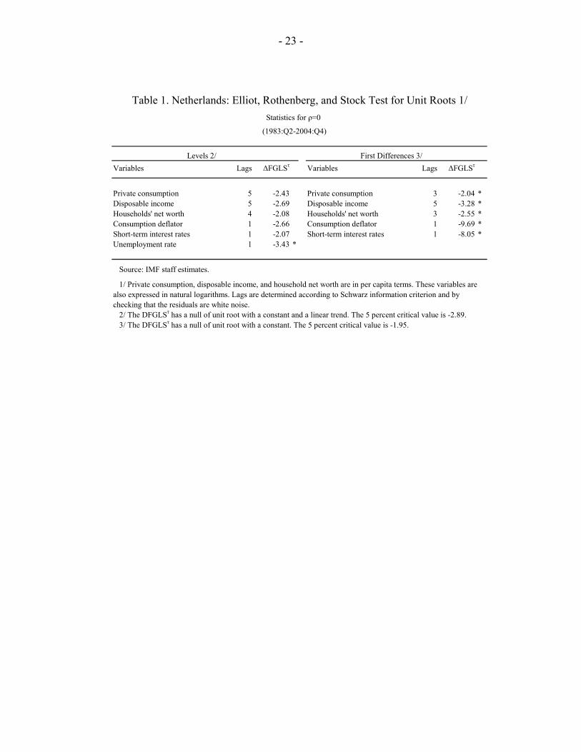
18. The series were tested for unit roots. In particular, the Elliot, Rothenberg, and Stock (1996) test was used. With a 95 percent confidence, all series except the unemployment rate contained a unit root (Table 1). In contrast, the first differences of the series were stationary. The unit root tests on the levels of the series were done including a constant and a deterministic trend; only a constant was included when testing the first differences of the series for unit roots. The number of lags for all tests were optimally chosen using the Schwarz information criterion.

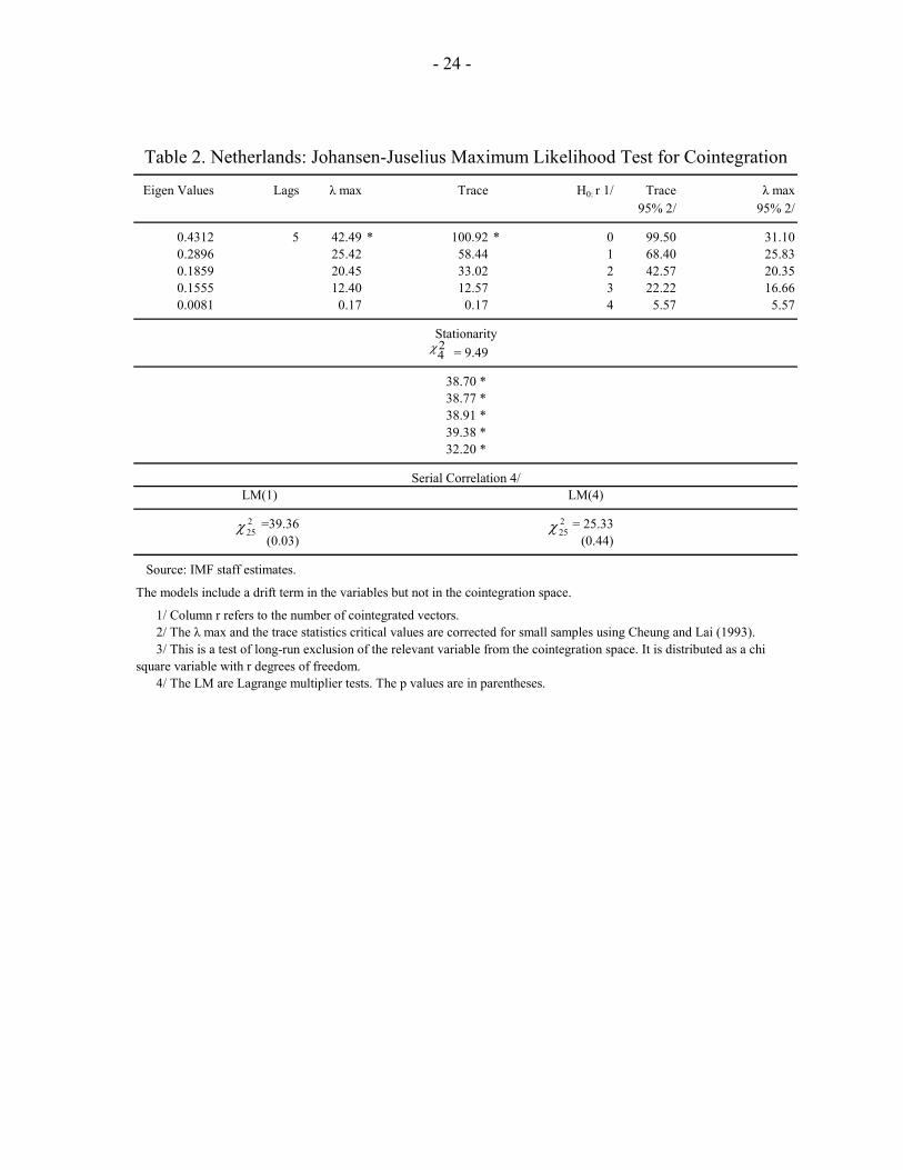
19. Next, consumption, disposable income, wealth, interest rates, and the unemployment rate were tested for cointegration. The Johansen-Juselius test, corrected for small sample bias, strongly rejected the no-cointegration hypothesis using the λmax or the trace statistic at the 95 percent level (Table 2).13 Residuals were white noise. While the λmax statistic could not reject the null hypothesis of one cointegrating vector against the alternative of two, its value (25.42) was very close to the corrected 95 percent confidence value (25.83). This is consistent with the difference in results between the univariate unit root test, which suggests that the unemployment rate is stationary, and the multivariate test of stationarity, which rejects the hypothesis of stationarity for all variables, including the unemployment rate. The estimation of the long-run consumption equation included the unemployment rate; it improved the overall fit of the equation.

D. The Long-Run Elasticities of the Model

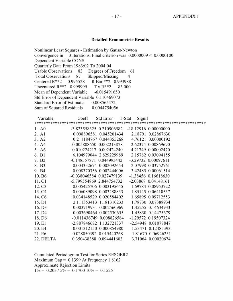
20. The econometric results support the view that sluggish private consumption so far this decade has been consistent with the behavior of some key consumption fundamentals (Figure 7). Equation (6) was estimated by the nonlinear dynamic least squares estimator of Phillips and Loretan (1991).14 The estimated form was:

( ) ( )1 1 ,k

t t t t t t t tt kC A Y X Y X A Y Xθ ω φ γ ρ θ ω ε− −=−

= + + + ∆ + ∆ + + + +∑ (7)

12 The share of population 65 years and older was also part of the sample, but was not included in the estimation as it was found to be an I(2) process.

13 The small sample bias correction followed Cheung and Lai (1993).

14 Their single-equation estimator is asymptotically equivalent to the maximum likelihood estimator of a full system of equations under Gaussian assumptions. The technique provides estimates that are statistically efficient and whose t-ratios can be used for inference in the usual way. Most importantly, the method takes into account both the serial correlation of the errors and the endogeneity of the regressors that is present when there is a cointegration relationship.

- 13 -

where Yt includes per capita real disposable income, per capita real net wealth and the interest rate, and Xt includes the unemployment rate and the inflation rate (measured by the consumption deflator). The last term is a serially uncorrelated error term with constant variance. 21. The long-run estimates of consumption are reported in the equation below.

3.82 0.10 0.21 0.01int 0.01 ,t t t t tC income wealth unemployment= − + + − − with ρ=0.35. (8)

The t-statistics are -18.13, 2.19, 4.76, -2.62, -4.22, and 3.71, respectively. The equilibrium correction term (ρ) is strongly significant.15 All the variables are significant at the 95 percent level. While there is some evidence of multicollinearity between real per capita disposable income and the real per capita net worth measure, this does not seem to be a serious problem.16 Inflation is never significant in the long run.17 The real interest rate is always significant and negative. Uncertainty, as proxied by the unemployment rate, plays a statistically significant role in explaining long-run consumption, though its economic magnitude is much lower than income or wealth.

22. While the long-run income elasticity is low, wealth effects are economically and statistically significant. The low long-run income elasticity likely reflects the inclusion of property income in real disposable income and the use of total consumption rather than nondurables consumption in the estimation.18 This explanation is all the more likely because the share of durables in total consumption has been consistently increasing since 1995Q1.19

15 Appendix 1 contains the complete estimates of equation (7). There is no serial correlation in the residuals as indicated by the cumulated periodogram test. As usual with the Phillips and Loretan estimator, the goodness of fit of the equation as measured by the centered R2 is very high.

16 A model that excludes wealth results in a higher income elasticity, but not significantly different from the value reported above. Moreover, the long-run parameters are superconsistent. 17 Inflation enters the short-run consumption dynamics with a positive sign. While empirical work often finds inflation to be significant with a negative sign, this is not always the case; and it is not even necessary from a theoretical viewpoint. A negative sign can be expected to the extent that inflation causes nonindexed assets to depreciate or that changes in inflation dominate changes in nominal interest rates. In any of those two cases, consumption will tend to fall because of a negative income effect. When the intertemporal substitution effect (i.e., ceteris paribus, inflation induces consumers to bring forward their consumption) outweighs the income effect, a positive coefficient may result.

18 Recall from footnote 1 that the household saving ratio is highly correlated with the share of property income in disposable income.

19 While nondurable expenditure and consumption largely coincide, durable expenditure and consumption are separate events in time. Expenditure on durables are typically made in longer discrete intervals, so habit persistence, duration, and convex adjustment costs are likely to play an important role. The impact of financing

(continued)

- 14 -

The wealth elasticity is somewhat higher than usual. The relatively large role of wealth suggests a liquid and efficient consumer credit market. Based on the sample average wealth-to-consumption ratio, the Dutch marginal propensity to consume out of real net wealth is about 5¼ cents to the euro. This is somewhat higher than the 4 cents to the dollar for the United States (for gross stock market wealth) and close to the United Kingdom’s 5 cents to the pound (for gross stock market wealth). The estimated wealth elasticity is consistent with results in Ludwig and Sløk (2002) who show that the Netherlands belongs to “market-based economies” to the extent that its wealth elasticity is comparable to Anglo-Saxon economies’ rather than to continental Europe’s bank-based economies (e.g., the wealth elasticity is less than 3 cents to the euro in France).20

23. Long-run consumption behavior has closely followed the behavior of its fundamentals, including the proxy for uncertainty. A comparison of long-run estimated consumption with actual consumption suggests that the latter caught up with the favorable fundamentals of the second half of the 1990s sometime in 2000. Since mid-2001, negative shocks to the factors that explain consumption reduced equilibrium long-run consumption, which reached a trough in 2003Q3. By the end of the sample period (Q4 2004), actual consumption appeared to have caught up with its long-run fundamentals.21

E. Concluding Remarks

24. This paper found that income, wealth, interest rates, and uncertainty (proxied by the unemployment rate) are the main determinants of total private consumption in the Netherlands. The relatively large role of real net wealth suggests a liquid and efficient credit market, facilitating consumption smoothing. It also suggests that Dutch consumers adjust their consumption quickly to persistent changes in their wealth.

25. With consumption having caught up with its fundamentals by the end of 2004, there are reasonable prospects for a pick up in consumption. In particular, private consumption can now be expected to accelerate with growth prospects improving and to the extent that the stock market and house prices boost wealth, and unemployment (and other sources of uncertainty generally) subside.

conditions is likely to also play a role on the timing of those purchases quite different from the role played in nondurables purchases. Durables consumption, defined as services out of the stock of durables, can be expected to be much smoother than expenditures. Therefore, it is to be expected that the marginal propensity to consume out of total consumption (i.e., consumption including durables) will be relatively lower than the marginal propensity to consume out of only nondurables.

20 Wealth elasticity estimates are frequently based on consumption equations that are restricted to nondurables consumption.

21 On average, consumption adjusts to its equilibrium level in about three quarters.

- 15 -

26. Further structural reforms could give a positive lift to consumption through other than mainstream channels. Consumer confidence is sensitive to developments in the stock market in the Netherlands. Thus, to the extent that structural reforms boost potential growth, consumption could not only be boosted directly, but also indirectly through confidence effects. In addition, enhancing the transparency of pension fund rules should reduce uncertainty about the present value of consumers’ expected income. Reduced uncertainty would increase the observed marginal propensity to consume out of income and wealth.

- 16 -

References Allais, O., L. Cadiou, and S. Dées, 2002, Defining Consumption Behavior in a Multi-Country

Model, Centre d’Etudes Prospectives et d’Informations Internationales, WP 01-02. Bayoumi, T., and H. Edison, 2003, Is Wealth Increasingly Driving Consumption? De

Nederlandsche Bank NV, DNB Staff Reports No.11. Boone, L., and N. Girouard, The Stock Market, the Housing Market and Consumer

Behaviour, OECD Economic Studies No. 35. Cheung, Y. W., and K. S. Lai, 1993, Finite Sample Sizes of Johansen’s Likelihood Ratio Test

for Cointegration, Oxford Bulletin of Economics and Statistics 55, pp. 313–28. Deaton, A., 1992, Understanding Consumption, Oxford: Clarendon Press. De Nederlandsche Bank NV, 2004: The Dutch Consumer: from Shopaholic to Enthusiastic

Saver, De Nederlandsche Bank Quarterly Bulletin, pp. 57–68, September. Elliott, G., T. J. Rothenberg, and J. Stock, 1996, Efficient Tests for an Autoregressive Unit

Root, Econometrica 64, pp. 813–36. Jansen, W. J., and N. J. Nahuis, 2003, The Stock Market and Consumer Confidence:

European Evidence, Economics Letters 79, pp. 89–98. Ludwig, A., and T. Sløk, 2002, The Impact of Changes in Stock Prices and House Prices on

Consumption in OECD Countries, International Monetary Fund, WP/02/01. Muellbauer, J,. and R. Lattimore, 1995, The Consumption Function: A Theoretical and

Empirical Overview, in H. Pesaran and M. Wickens (eds.), Handbook of Applied Econometrics, pp. 221–301, Oxford: Blackwell.

Phillips, P., and M. Loretan, 1991, Estimating Long-Run Economic Equilibria, Review of

Economic Studies 58, pp. 407–436. Schule, W., 2004, Household Consumption in France, France: Selected Issues, International

Monetary Fund, pp. 5–26.

- 17 - APPENDIX 1

Detailed Econometric Results Nonlinear Least Squares - Estimation by Gauss-Newton Convergence in 3 Iterations. Final criterion was 0.0000009 < 0.0000100 Dependent Variable CONS Quarterly Data From 1983:02 To 2004:04 Usable Observations 83 Degrees of Freedom 61 Total Observations 87 Skipped/Missing 4 Centered R**2 0.995528 R Bar **2 0.993988 Uncentered R**2 0.999999 T x R**2 83.000 Mean of Dependent Variable -6.015491650 Std Error of Dependent Variable 0.110469073 Standard Error of Estimate 0.008565472 Sum of Squared Residuals 0.0044754056 Variable Coeff Std Error T-Stat Signif *************************************************************************** 1. A0 -3.823558325 0.210906582 -18.12916 0.00000000 2. A1 0.098896581 0.045201434 2.18791 0.02867630 3. A2 0.211184767 0.044355268 4.76121 0.00000192 4. A4 -0.005808650 0.002213878 -2.62374 0.00869690 5. A6 -0.010224217 0.002424240 -4.21749 0.00002470 6. B1 6.104979044 2.829229989 2.15782 0.03094155 7. B2 -0.148357871 0.044993442 -3.29732 0.00097611 8. B3 0.004352674 0.002092654 2.07998 0.03752761 9. B4 0.008370356 0.002444006 3.42485 0.00061514 10. B6 -0.038046584 0.027479139 -1.38456 0.16618630 11. C1 -5.799554869 2.844754732 -2.03868 0.04148161 12. C3 0.005425706 0.003195645 1.69784 0.08953722 13. C4 0.006089098 0.003288833 1.85145 0.06410537 14. C6 0.034148529 0.020584402 1.65895 0.09712553 15. D1 2.111353413 1.181310233 1.78730 0.07388934 16. D3 0.003719931 0.002560969 1.45255 0.14634933 17. D4 0.003690464 0.002530655 1.45830 0.14475679 18. D6 -0.011436749 0.008826584 -1.29572 0.19507324 19. E1 -2.887846682 1.132721337 -2.54948 0.01078847 20. E4 -0.001312150 0.000854980 -1.53471 0.12485393 21. E6 0.028050392 0.015440268 1.81670 0.06926251 22. DELTA 0.350438388 0.094441603 3.71064 0.00020674 Cumulated Periodogram Test for Series RESGER2 Maximum Gap = 0.1399 At Frequency 1.8162 Approximate Rejection Limits 1% = 0.2037 5% = 0.1700 10% = 0.1525

- 18 - APPENDIX I

Variables are: A0 = Constant A1 = Real per capita disposable income A2 = Real household's net worth per capita A4 = 3-Month real interest rate A6 = Unemployment rate B1 = Change in income B2 = Change in net worth B3 = Consumption deflator inflation B4 = Change in 3-month interest rates B6 = Change in unemployment rate C1 = Change in income, lagged once C3 = Inflation, lagged once C4 = Change in 3-month interest rates, lagged once C6 = Change in unemployment rate, lagged once D1 = Change in income, lagged twice D3 = Inflation, lagged twice D4 = Change in 3-month interest rates, lagged twice D6 = Change in unemployment rate, lagged twice E1 = Change in income, lead once E4 = Change in 3-month interest rates, lead once E6 = Change in unemployment rate, lead once DELTA = Long-run equilibrium adjustment parameter

- 19 -

Figure 1. Netherlands: Consumption, Income, and Net Worth

(Average Annual Growth Rates)

-6

-3

0

3

6

9

12

1985Q1 1987Q1 1989Q1 1991Q1 1993Q1 1995Q1 1997Q1 1999Q1 2001Q1 2003Q1

Real per capita disposable incomeReal per capita households' net worthReal private total consumption per capita

Sources: DNB; and IMF staff calculations.

2

4

6

8

10

12

1984Q2 1986Q2 1988Q2 1990Q2 1992Q2 1994Q2 1996Q2 1998Q2 2000Q2 2002Q2 2004Q2

Sources: DNB; and IMF staff calculations.

Figure 2. Netherlands: Unemployment Rate

- 20 -

Figure 3. Netherlands: Interest Rates and Stock Market Returns

0

1

2

3

4

5

6

7

8

1984Q1 1986Q1 1988Q1 1990Q1 1992Q1 1994Q1 1996Q1 1998Q1 2000Q1 2002Q1 2004Q1-60

-40

-20

0

20

40

60

80

Three-month real interest rates (in percent)

Gross stock market returns (right scale, averageannual growth rate)

Sources: DNB; and IMF staff calculations.

0

100

200

300

400

500

600

700

800

1983M1 1986M1 1989M1 1992M1 1995M1 1998M1 2001M1 2004M1

Sources: DNB; and IMF staff calculations.

Figure 4. Netherlands: Stock Market Price Index

- 21 -

Figure 5. Netherlands: Real House Prices(Average Annual Growth Rates)

-5

0

5

10

15

20

1984Q1 1986Q1 1988Q1 1990Q1 1992Q1 1994Q1 1996Q1 1998Q1 2000Q1 2002Q1 2004Q1

Source: Kadaster.

Figure 6. Netherlands: Real Household Net Worth/ Income 1/

35

40

45

50

55

1984Q1 1986Q1 1988Q1 1990Q1 1992Q1 1994Q1 1996Q1 1998Q1 2000Q1 2002Q1 2004Q1

Sources: DNB; and IMF staff calculations.

- 22 -

-6.3

-6.2

-6.1

-6.0

-5.9

-5.8

-5.7

-5.6

1983Q2 1985Q2 1987Q2 1989Q2 1991Q2 1993Q2 1995Q2 1997Q2 1999Q2 2001Q2 2003Q2

Consumption

Long-Run Consumption

Sources: DNB; and IMF staff calculations.

Figure 7. Netherlands: Consumption and Estimated Long-Run Consumption(Levels; in natural logs)

- 23 -

Variables Lags ∆FGLSτ Variables Lags ∆FGLSτ

Private consumption 5 -2.43 Private consumption 3 -2.04 *Disposable income 5 -2.69 Disposable income 5 -3.28 *Households' net worth 4 -2.08 Households' net worth 3 -2.55 *Consumption deflator 1 -2.66 Consumption deflator 1 -9.69 *Short-term interest rates 1 -2.07 Short-term interest rates 1 -8.05 *Unemployment rate 1 -3.43 *

Source: IMF staff estimates.

1/ Private consumption, disposable income, and household net worth are in per capita terms. These variables arealso expressed in natural logarithms. Lags are determined according to Schwarz information criterion and bychecking that the residuals are white noise.

2/ The DFGLSτ has a null of unit root with a constant and a linear trend. The 5 percent critical value is -2.89.3/ The DFGLSτ has a null of unit root with a constant. The 5 percent critical value is -1.95.

Table 1. Netherlands: Elliot, Rothenberg, and Stock Test for Unit Roots 1/

Levels 2/ First Differences 3/

Statistics for ρ=0

(1983:Q2-2004:Q4)

- 24 -

Eigen Values Lags λ max Trace H0: r 1/ Trace λ max95% 2/ 95% 2/

0.4312 5 42.49 * 100.92 * 0 99.50 31.100.2896 25.42 58.44 1 68.40 25.830.1859 20.45 33.02 2 42.57 20.350.1555 12.40 12.57 3 22.22 16.660.0081 0.17 0.17 4 5.57 5.57

LM(1)

=39.36(0.03) (0.44)

Source: IMF staff estimates.

The models include a drift term in the variables but not in the cointegration space.

1/ Column r refers to the number of cointegrated vectors.2/ The λ max and the trace statistics critical values are corrected for small samples using Cheung and Lai (1993).3/ This is a test of long-run exclusion of the relevant variable from the cointegration space. It is distributed as a chi

square variable with r degrees of freedom.4/ The LM are Lagrange multiplier tests. The p values are in parentheses.

= 25.33

Serial Correlation 4/ LM(4)

Table 2. Netherlands: Johansen-Juselius Maximum Likelihood Test for Cointegration

Stationarity = 9.49

32.20 *

38.70 *38.77 *38.91 *39.38 *

225χ 2

25χ

24χ

- 25 -

III. HOUSE PRICES IN THE NETHERLANDS22

A. Introduction

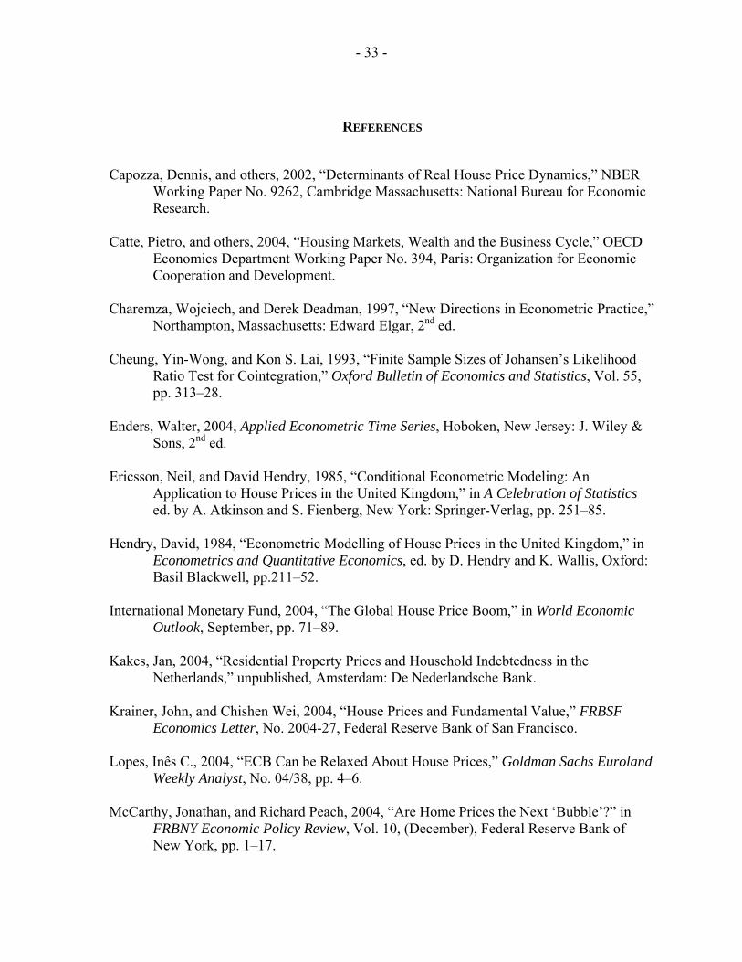
27. Between 1995 and 2001, average Dutch house prices rose by almost 80 percent in real terms, raising concerns about the sustainability of the resulting price levels. Various observers have warned that house prices appear to be out of line with economic fundamentals, and some—notably ING, a large commercial bank and mortgage supplier—have suggested that a substantial correction of prices could be imminent.

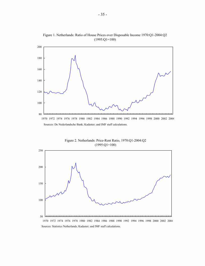
28. There is some historical justification for such concerns. In the late 1970s, the Netherlands also experienced an episode of rapidly rising house prices, which was then followed by a painful complete reversal of the price gains in the early 1980s.

29. Some indicators seem to support the claims that house prices have been divorced from market fundamentals. A basic—and rather crude—measure of housing affordability that is used by analysts is the ratio of house prices to the disposable income of households. Since 1995, this ratio has risen by more than 50 percent in the Netherlands, suggesting a sharp decline in the affordability of housing (Figure 1). This development certainly appears reminiscent of the housing boom of the late 1970s. And, at its current level, the ratio lies some 40 percent above its 30-year average.

30. Another simple measure of the relative valuation of housing is the ratio of house prices to the going rent. This “price-rent ratio” is broadly comparable to the “price-earnings ratio” that is used to assess the valuation of stocks; it measures the return on investment in housing and says something about the attractiveness of residential property as an asset class. On this measure, concerns about overvaluation appear even more well-founded than those arising from the affordability ratio. The price-rent ratio has risen by more than 75 percent since 1995, and its current level is more than 50 percent above the average of the past 30 years (Figure 2).

31. Housing supply conditions in the Netherlands may make the market prone to an overshooting of prices. The Netherlands is one of the most densely populated countries in the world (with 478 people per square kilometer), undeveloped land is in short supply, and zoning laws tend to be very strict. Consequently, the supply elasticity of housing is usually regarded as very low (Swank, Kakes, and Tieman, 2002, provide empirical evidence). Studies for regional markets in the United States have found that low supply elasticities are associated with a tendency for prices to overshoot (see below). However, some observers in the Netherlands see the structural supply shortage as a factor that supports and justifies the current high house prices (e.g., Rabobank, 2003).

22 Prepared by David Hofman.

- 26 -

32. Thus far, in contrast to the experience of the early 1980s, the Dutch housing market seems to be making a soft landing. After a period of exceptionally rapid growth, economic conditions started to deteriorate in 2001 on the heels of the global collapse of equity prices and the subsequent slowdown of the world economy. The Dutch downturn was compounded by a unusually sharp contraction of domestic consumption, and in 2003 average annual growth turned negative for the first time in 20 years. While house price increases have moderated substantially during this period, average prices have so far not shown any decline except at the very high end of the market.

33. Against this background, the question remains of whether the remarkable rise in house prices has been the result of a change in fundamental conditions, the reflection of a catch-up process—that is, an adjustment toward a long-run equilibrium level—or an unsustainable upward deviation from their equilibrium level, as is suggested by the affordability and price-rent ratios. In the latter case, a correction of house prices would be expected at some point.

34. This paper examines the extent to which the Dutch housing boom can be explained by fundamentals. Section B briefly discusses the relevant literature in the field of housing markets. Then, in Section C, a basic error-correction model of house prices is developed. Sections D and E discuss the data series and various econometric issues. Section F presents the empirical results from the analysis, followed by some concluding remarks in Section G.

B. Brief Review of the Literature

35. An extensive empirical literature examines house price movements in terms of their fundamentals. However, there is no clear consensus on the theoretical framework that should underpin such exercises.

36. One strand of the literature views housing primarily as a durable consumption good and examines the relationship of house prices to the real economy and demand factors such as general economic conditions and housing affordability. For instance, Hendry (1984) models the market for “second-hand” housing in the United Kingdom using real disposable income, interest rates, retail prices, and mortgage credit as explanatory variables. Also included is a cubic lagged house price term in the short-run dynamics, to pick up bubble behavior; the resulting model performs well in tracking the volatile British housing market. Similarly, Vladkova Hollar (2003) estimates an equation for house prices, again in the United Kingdom, using an error-correction model with disposable income and the real interest rate as the only other variables. Both variables appear in the long-run relationship as well as in the short-term dynamics of the model (together with the lagged house prices themselves), and provide it with considerable explanatory power.

37. Other research focuses primarily on the function of housing as an asset or investment. These studies typically compare house prices to developments in rents and the rates of return in other classes of assets. An example of such an approach is a study by Krainer and Wei (2004) that analyzes house prices in the United States using concepts from the finance

- 27 -

literature. Specifically, they decompose the increase in the price-rent ratio into two parts: one that is related to expected future rent increases, and another that corresponds to expected increases in house prices, concluding that the latter part is the main driver of the U.S. price-rent ratio.

38. From a theoretical perspective, it would appear desirable to include a supply-side in any model for the housing market. As in the above examples, however, supply factors (e.g., building costs) are frequently omitted in the literature. Indeed, there can be a good reason for doing so, in particular for markets where the supply elasticity is deemed to be very low. In such cases, at least in the short term, housing supply is essentially given and equal to the existing housing stock. The United Kingdom, for example, is often considered as a country where supply restrictions are binding, and therefore various studies for the U.K.—including the ones quoted above—do not attempt to model supply factors (see also Muellbauer and Murphy, 1997).23 In contrast, many studies for the United States do include supply factors (e.g., McCarthy and Peach, 2004). One interesting result from this literature, which is also relevant for cases where the supply elasticity is low, is that the relative responsiveness of supply can affect the volatility of house prices. In a panel data survey covering 65 metropolitan areas in the United States, Capozza and others (2002) find that high building costs—related, inter alia, to barriers to new construction—increase the persistence in house prices and reduce the speed of mean reversion, thus creating fertile ground for price overshooting and speculative bubbles.

39. From the perspective of housing as a store of wealth, (expected) inflation is another factor that can affect house prices. In a cross-country study, including multiple variables, Tsatsaronis and Zhu (2004) find that on average across the countries in their sample, inflation explains more than half of the total variation in house prices. This finding could also be related to the common practice of financing houses with debt, which is fixed in nominal terms, and to the attractiveness of such financing in periods of high inflation.

40. Some recent work also includes wealth effects from stock market developments in housing demand equations. One example is Sutton (2002), who relates house prices in a sample of industrial countries to fluctuations in national income, interest rates, and stock prices, and finds a significant contribution from the last variable. Similarly, for the Netherlands, Van den End and Kakes (2002) find a positive long-run correlation between the stock market and house prices. The relationship is found to be complex and running in both directions, but it seems strongest from stock prices to house prices, at a two-three year lag. As the Dutch stock market has lost about half of its value since 2000, this finding suggests that there is substantial scope for downward movement in current house price levels.

41. Few recent studies focus exclusively on the Dutch housing market, such as the one by Van den End and Kakes discussed above. The main other study is a recent analysis by 23 Of course, there are studies on the United Kingdom that do include supply factors. For example, Ericsson and Hendry (1985) focus specifically on the economics of house building.

- 28 -

Verbruggen and others (2005), who explain Dutch house price movements between 1980 and 2003 using an error-correction model with several variables, including household wealth. They conclude that current Dutch house prices are “somewhat” overvalued. They also find that adjustment of actual house prices to their equilibrium level takes place faster when the equilibrium price is on the rise than when it is falling (i.e., they find that house prices are sticky downwards).

42. These specific papers aside, the Netherlands has been included in various recent cross-country studies on housing. Most of these find that Dutch house prices are currently overvalued by some margin. Research by PricewaterhouseCoopers (2002) finds that Dutch house prices are influenced by past changes in long-term interest rates, inflation, the amount of new construction, and past house price changes. But their model fails to explain the strong price increases in 1999–2001, which they conclude are likely to represent speculative behavior. Lopes (2004), using a model based on real disposable income growth, mortgage interest rates, and the equity market, finds that Dutch house prices are overvalued by about 10 percent, a result that is broadly confirmed by the IMF (2004), which also includes population and credit growth as explanatory variables in its analysis. Incidentally, consistent with the recent strength of house prices during the economic downturn, Catte and others (2004) find that the correlation of house prices and the business cycle is weak in the Netherlands.

C. The Conceptual Framework

43. Since the supply of new housing is very inelastic in the Netherlands, this paper will focus exclusively on demand factors to explain the behavior of prices. Some empirical backing for this choice can be found in Van Rooij (1999), who fails to find any long-run effects of housing supply on house prices in the Netherlands. Consistent with data properties (see below), we employ an error-correction model, which allows a distinction to be made between short-term dynamics (including possible persistence in house prices) and long-run relationships that might exist between house prices and their main determinants. The broad framework is given by

t

k

iititt ZZ εµ ++∆Ζ⋅Γ+⋅Π=∆ ∑

−

=−−

1

11 (1)

where Z is a vector containing the n variables of the system, matrix Π captures information on the long-run relationships among the variables in Z, matrix Γ contains information on the lagged variables, and µ is a vector with constants.

44. For the vector Z, we considered a range of variables including, besides house prices, the disposable income of households, the mortgage interest rate, consumer price inflation, and rents (as measured by the rent component in the Dutch consumer price index). In addition, we examined the variables in both nominal and real terms. Using a “General-to-Specific” modeling approach (see e.g., Enders, 2004, or Charemza and Deadman, 1997, for a

- 29 -

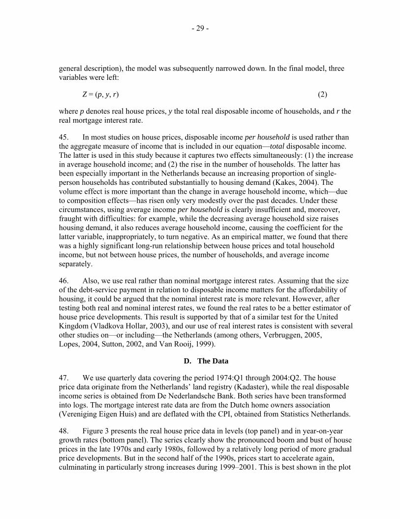
general description), the model was subsequently narrowed down. In the final model, three variables were left:

Z = (p, y, r) (2)

where p denotes real house prices, y the total real disposable income of households, and r the real mortgage interest rate.

45. In most studies on house prices, disposable income per household is used rather than the aggregate measure of income that is included in our equation—total disposable income. The latter is used in this study because it captures two effects simultaneously: (1) the increase in average household income; and (2) the rise in the number of households. The latter has been especially important in the Netherlands because an increasing proportion of single-person households has contributed substantially to housing demand (Kakes, 2004). The volume effect is more important than the change in average household income, which—due to composition effects—has risen only very modestly over the past decades. Under these circumstances, using average income per household is clearly insufficient and, moreover, fraught with difficulties: for example, while the decreasing average household size raises housing demand, it also reduces average household income, causing the coefficient for the latter variable, inappropriately, to turn negative. As an empirical matter, we found that there was a highly significant long-run relationship between house prices and total household income, but not between house prices, the number of households, and average income separately.

46. Also, we use real rather than nominal mortgage interest rates. Assuming that the size of the debt-service payment in relation to disposable income matters for the affordability of housing, it could be argued that the nominal interest rate is more relevant. However, after testing both real and nominal interest rates, we found the real rates to be a better estimator of house price developments. This result is supported by that of a similar test for the United Kingdom (Vladkova Hollar, 2003), and our use of real interest rates is consistent with several other studies on—or including—the Netherlands (among others, Verbruggen, 2005, Lopes, 2004, Sutton, 2002, and Van Rooij, 1999).

D. The Data

47. We use quarterly data covering the period 1974:Q1 through 2004:Q2. The house price data originate from the Netherlands’ land registry (Kadaster), while the real disposable income series is obtained from De Nederlandsche Bank. Both series have been transformed into logs. The mortgage interest rate data are from the Dutch home owners association (Vereniging Eigen Huis) and are deflated with the CPI, obtained from Statistics Netherlands.

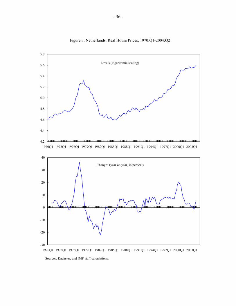
48. Figure 3 presents the real house price data in levels (top panel) and in year-on-year growth rates (bottom panel). The series clearly show the pronounced boom and bust of house prices in the late 1970s and early 1980s, followed by a relatively long period of more gradual price developments. But in the second half of the 1990s, prices start to accelerate again, culminating in particularly strong increases during 1999–2001. This is best shown in the plot

- 30 -

of the year-on-year growth rates. This presentation also reveals, however, that, even while the level of real house prices has now surpassed that of the late 1970s, the growth rates during the latest “boom” have been appreciably more moderate. Since 2001, the growth rate of house prices has slowed quite abruptly.

49. Figure 4 presents the other two data series: disposable income and the mortgage interest rate. The real disposable income measure is shown in the top panel, together with its breakdown into income per household and the number of households. Over the range of the sample, it is clear that important composition effects are at play: the number of households is increasing steadily—and at a much faster pace than would be explained by population growth—while real income per household is almost flat, which seems at odds with the sizable increases in overall prosperity recorded over this 30-year period. Looking at the aggregate series, disposable income appears to have reacted quite strongly to the turning points in the business cycle, which broadly coincided with the turn of each decade. For the bust of the early 1980s, as well as for the recent downturn, this accords well with the developments in the housing market. For the developments in the early 1990s, however, the link between income and house prices is less pronounced.

50. The bottom panel shows the real mortgage interest rate, together with its breakdown into the nominal rate and inflation. The figure illustrates how real interest rates took off around 1976 on account of rapidly falling inflation and, after peaking in 1987, gradually descended during the 1990s in line with developments in nominal interest rates.

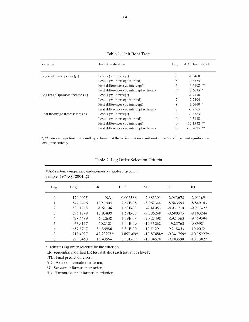
51. All three data series are I(1), i.e., they contain a unit root in levels, but not in their first differences. For each variable, the nonstationarity condition was tested using the augmented Dickey-Fuller (ADF) test. The tests were conducted with a constant in the test specification and both including and excluding a trend. The lag length was determined on the basis of the Schwarz information criterion. The test results are summarized in Table 1.

52. It must be noted that the evidence with regards to the order of integration of the real disposable income variable is mixed. While the ADF test rejects the null hypothesis of a unit root in the first differences at the 5 percent level when only a constant is included in the test, it fails to reject when a trend is added. In principle, this suggests that the variable might possibly be integrated of a higher order than one. Nonetheless, we accept disposable income to be I(1), since also in the second test specification, the test statistic is very close to the 5 percent critical value, and because on theoretical grounds, there is no reason to suspect integration of a higher order for this variable.

E. Econometric Issues and Hypothesis Tests

53. A vector autoregression system was constructed with the three variables (p, y, r) over the period 1974:Q1–2004:Q2. The appropriate lag length of the system was determined on the basis of a range of widely-used selection criteria. The results of these lag order tests are summarized in Table 2. Unanimously, the criteria select an order of seven lags.

- 31 -

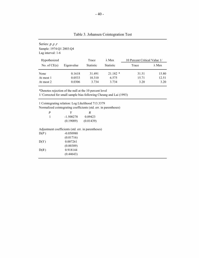
54. Subsequently, we tested for possible cointegration between the variables in the system using the Johansen cointegration test. The test results are shown in Table 3. While the trace statistic is too close to the critical value to be conclusive, the λmax value strongly indicates the existence of one cointegrating equation, including all three variables, at the 10 percent level. The coefficients of the variables in the cointegrating equation are very significant and their signs are consistent with economic theory. On the basis of this result, the error-correction model was estimated. In the initial system, the cointegrating vector was significant only in the house price and the mortgage rate equations. The disposable income variable was found to be weakly exogenous, and the income equation could be dropped without loss of information, leaving a two-equation system.

55. With two equations, each containing a constant, an error correction term, and six lags for each of the three variables, the resulting system comprised 40 coefficients. For parsimony, and because various coefficients in the system were not significant, the number of variables in the system was then reduced by applying Wald tests to various groupings of variables. While it was not possible to eliminate complete lags from the system without substantially reducing its explanatory power, one variable could be omitted from each equation. Specifically, the Wald tests indicated that the lagged values of the interest rate were not significant in the short-term dynamics of the house price equation. Similarly, the lagged house prices did not appear to be a short-term determinant of the interest rate.

F. Empirical Results

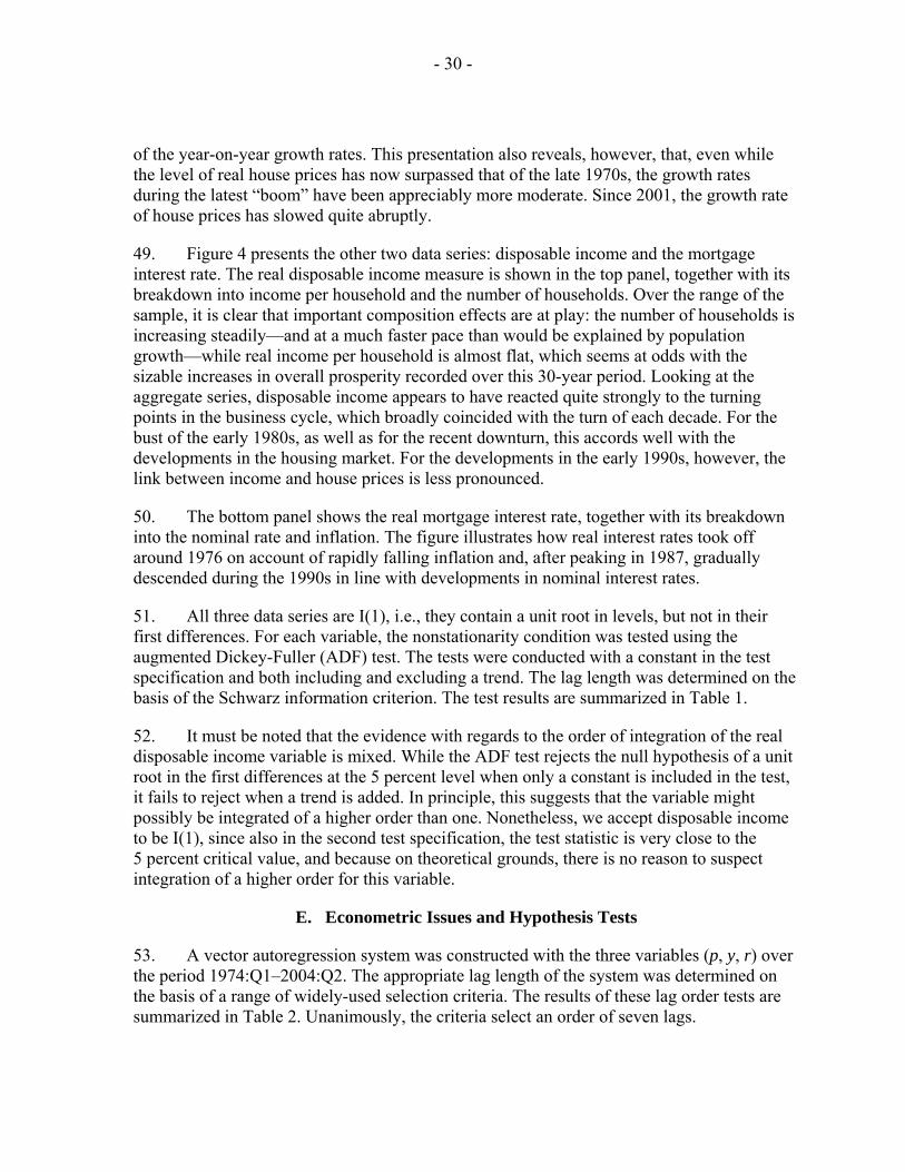
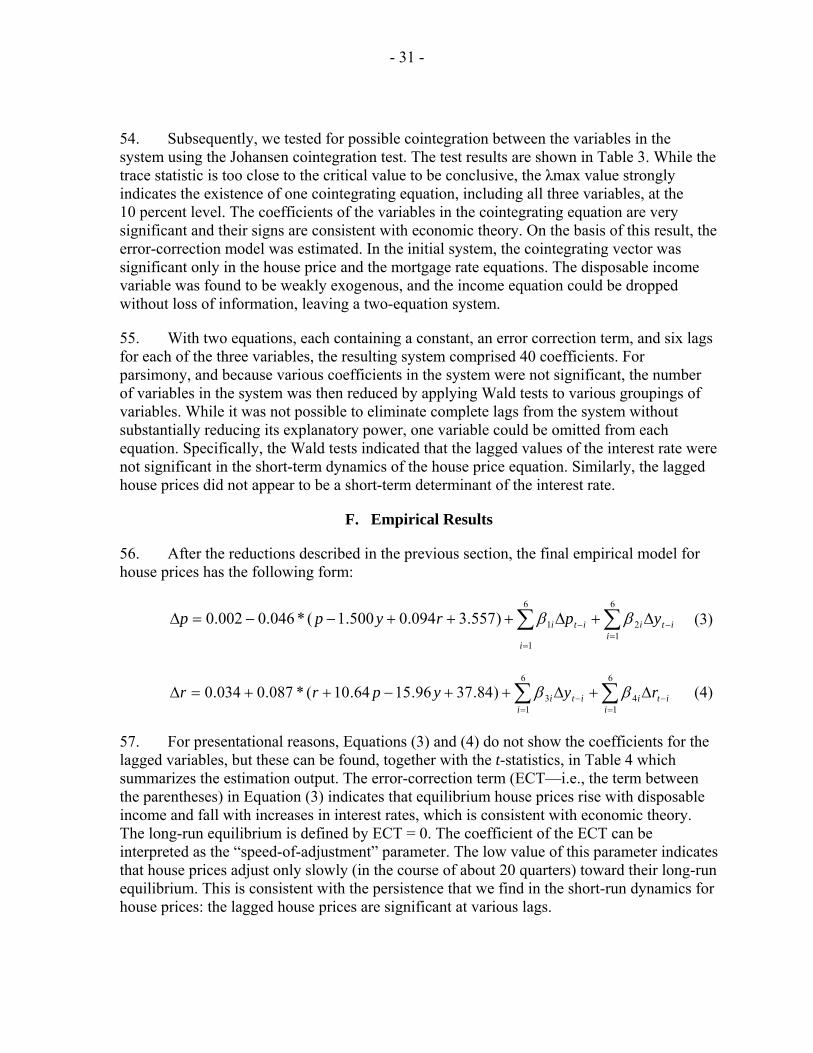
56. After the reductions described in the previous section, the final empirical model for house prices has the following form:

∑ ∑=

=−− ∆+∆+++−−=∆

6

1

6

121)557.3094.0500.1(*046.0002.0

ii

itiiti yprypp ββ (3)

∑∑=

−=

− ∆+∆++−++=∆6

14

6

13)84.3796.1564.10(*087.0034.0

iiti

iiti ryyprr ββ (4)

57. For presentational reasons, Equations (3) and (4) do not show the coefficients for the lagged variables, but these can be found, together with the t-statistics, in Table 4 which summarizes the estimation output. The error-correction term (ECT—i.e., the term between the parentheses) in Equation (3) indicates that equilibrium house prices rise with disposable income and fall with increases in interest rates, which is consistent with economic theory. The long-run equilibrium is defined by ECT = 0. The coefficient of the ECT can be interpreted as the “speed-of-adjustment” parameter. The low value of this parameter indicates that house prices adjust only slowly (in the course of about 20 quarters) toward their long-run equilibrium. This is consistent with the persistence that we find in the short-run dynamics for house prices: the lagged house prices are significant at various lags.

- 32 -

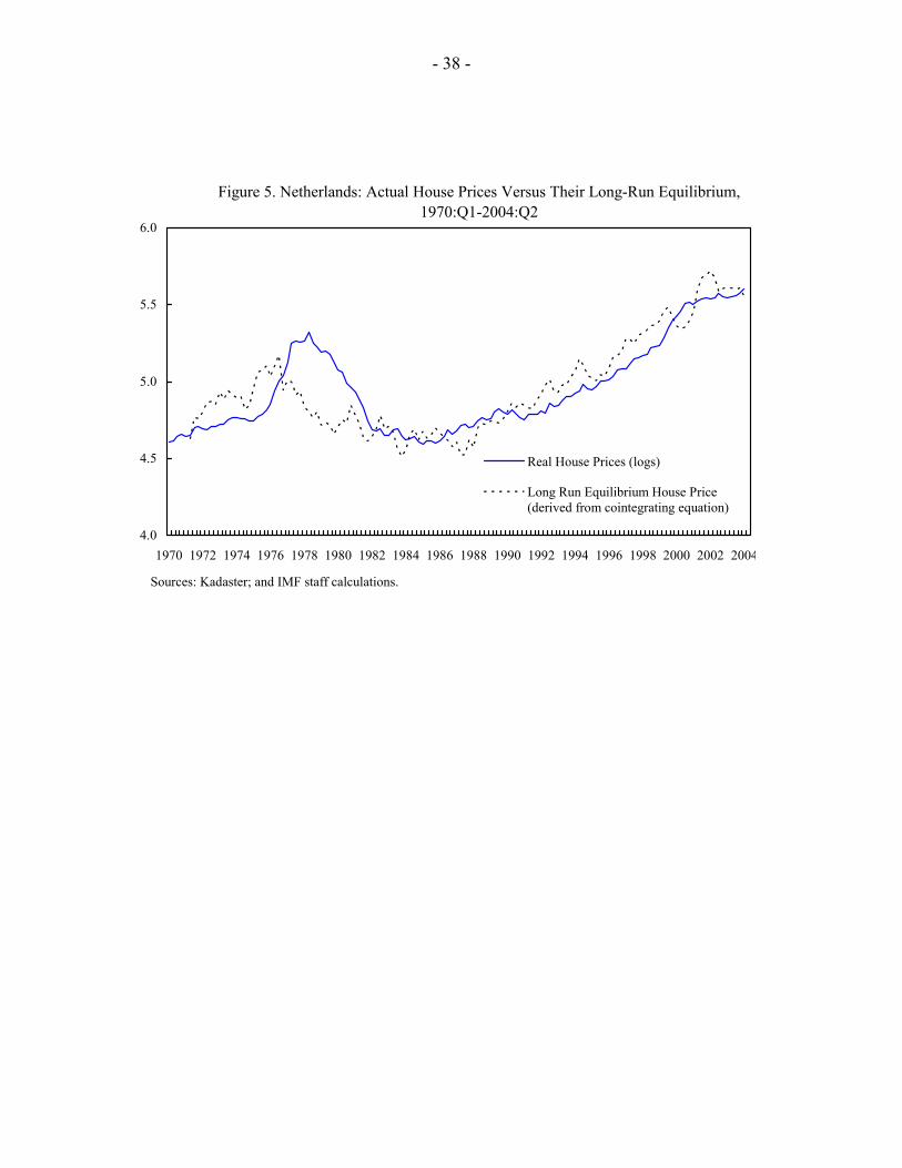
58. In order to answer the question of whether house prices are overvalued or not, in Figure 5 we plot the equilibrium house price as derived from the cointegrating equation and compare it with actual prices. The picture that emerges is striking. For the boom-bust episode of the late 1970s/early 1980s, it is still clear that prices were way out of line with fundamentals. In the second half of the 1970s, house prices rose, with a considerable lag, in response to an actual rise in the equilibrium price that was associated with increasing disposable income and declining mortgage rates. However, around 1976, the favorable environment of low real interest rates started to change as inflation fell rapidly in the aftermath of the first oil crisis, while nominal interest rates rose. This change in fundamentals was initially ignored in the market, and house prices continued to rise through 1979. By that time, however, disposable income had also stopped growing, and reality finally set in. House prices fell in order to realign with their fundamental value, a process that was completed around 1982.

59. Turning to recent periods, our analysis does not show an upward deviation from fundamentals. In fact, for most of the 1990s, actual house prices were below their long-run equilibrium, although there has been some catching-up in the last few years. Overall, actual house prices appear to have moved largely in line with their fundamental value—that is, in line with developments in total disposable income and interest rates. Apparently, the gradual decline of interest rates during the 1990s has had a large positive impact on the affordability of housing, which—in combination with a steady increase in total disposable income—has justified the rapid increases in house prices.

60. However, by no means does this imply that house prices are secure at their current levels. Indeed, fundamentals may change—as they did in the late 1970s. A key feature of our estimated equilibrium price is that it is quite volatile. Even small changes in income or interest rates have a relatively large impact on the fundamental value of housing. For example, it can be calculated on the basis of our results that a one percentage point increase in the real interest rate reduces the long-run equilibrium house price by about 10 percent. However, the short-term volatility of the fundamental value is normally not reflected in actual house prices because of the slow pace of adjustment.

G. Concluding Remarks

61. As was shown above, we fail to find evidence for a deviation from fundamentals in the current Dutch housing market. There is only limited comfort in this finding, though, because our analysis also shows that the equilibrium price of housing can change quite rapidly with developments in income and interest rates. The current weaknesses in disposable income growth therefore pose significant risks to the housing market, and if interest rates were to rise substantially in the period ahead, house prices may still fall.

- 33 -

REFERENCES

Capozza, Dennis, and others, 2002, “Determinants of Real House Price Dynamics,” NBER

Working Paper No. 9262, Cambridge Massachusetts: National Bureau for Economic Research.

Catte, Pietro, and others, 2004, “Housing Markets, Wealth and the Business Cycle,” OECD

Economics Department Working Paper No. 394, Paris: Organization for Economic Cooperation and Development.

Charemza, Wojciech, and Derek Deadman, 1997, “New Directions in Econometric Practice,”

Northampton, Massachusetts: Edward Elgar, 2nd ed. Cheung, Yin-Wong, and Kon S. Lai, 1993, “Finite Sample Sizes of Johansen’s Likelihood

Ratio Test for Cointegration,” Oxford Bulletin of Economics and Statistics, Vol. 55, pp. 313–28.

Enders, Walter, 2004, Applied Econometric Time Series, Hoboken, New Jersey: J. Wiley &

Sons, 2nd ed. Ericsson, Neil, and David Hendry, 1985, “Conditional Econometric Modeling: An

Application to House Prices in the United Kingdom,” in A Celebration of Statistics ed. by A. Atkinson and S. Fienberg, New York: Springer-Verlag, pp. 251–85.

Hendry, David, 1984, “Econometric Modelling of House Prices in the United Kingdom,” in

Econometrics and Quantitative Economics, ed. by D. Hendry and K. Wallis, Oxford: Basil Blackwell, pp.211–52.

International Monetary Fund, 2004, “The Global House Price Boom,” in World Economic

Outlook, September, pp. 71–89. Kakes, Jan, 2004, “Residential Property Prices and Household Indebtedness in the

Netherlands,” unpublished, Amsterdam: De Nederlandsche Bank. Krainer, John, and Chishen Wei, 2004, “House Prices and Fundamental Value,” FRBSF

Economics Letter, No. 2004-27, Federal Reserve Bank of San Francisco. Lopes, Inês C., 2004, “ECB Can be Relaxed About House Prices,” Goldman Sachs Euroland

Weekly Analyst, No. 04/38, pp. 4–6. McCarthy, Jonathan, and Richard Peach, 2004, “Are Home Prices the Next ‘Bubble’?” in

FRBNY Economic Policy Review, Vol. 10, (December), Federal Reserve Bank of New York, pp. 1–17.

- 34 -

Muellbauer, John, and Anthony Murphy, 1997, “Booms and Busts in the UK Housing Market,” The Economic Journal, Vol. 107, (November), pp. 1701–27.

PricewaterhouseCoopers, 2002, “European House Prices,” European Economic Outlook,

(May), pp. 19–29. Rabobank, 2003, Residential Property Market Quarterly, No. 4 (November 6), Utrecht:

Rabobank. Sutton, Gregory, 2002, “Explaining Changes in House Prices,” BIS Quarterly Review,

(September), Basel: Bank for International Settlements, pp. 46–55. Swank, Job, Jan Kakes, and Alexander Tieman, 2002, “The Housing Ladder, Taxation, and

Borrowing Constraints,” DNB Working Paper No. 2002/9, Amsterdam: De Nederlandsche Bank.

Tsatsaronis, Kostas, and Haibin Zhu, 2004, “What Drives Housing Price Dynamics: Cross

Country Evidence,” BIS Quarterly Review (March), Basel: Bank for International Settlements, pp. 65–78.

Van den End, Jan Willem and Jan Kakes, 2002, “The Relationship Between Stock Prices and

House Prices,” unpublished, Amsterdam: De Nederlandsche Bank. Van Rooij, Maarten, 1999, “De huizenprijsontwikkeling in Nederland: een analyse en de

economische effecten,” DNB Working Paper No. 583, Amsterdam: De Nederlandsche Bank.

Verbruggen, Johan, and others, 2005, “Welke factoren bepalen de ontwikkeling van de

huizenprijs in Nederland?, ” CPB document No. 81, Den Haag: CPB. Vladkova Hollar, Ivanna, 2003, “An Analysis of House Prices in the United Kingdom,” in

IMF Country Report No. 03/47, pp. 5–14.

- 35 -

Figure 1. Netherlands: Ratio of House Prices over Disposable Income 1970:Q1-2004:Q2(1995:Q1=100)

80

100

120

140

160

180

200

1970 1972 1974 1976 1978 1980 1982 1984 1986 1988 1990 1992 1994 1996 1998 2000 2002 2004

Sources: De Nederlandsche Bank; Kadaster; and IMF staff calculations.

Figure 2. Netherlands: Price-Rent Ratio, 1970:Q1-2004:Q2(1995:Q1=100)

50

100

150

200

250

1970 1972 1974 1976 1978 1980 1982 1984 1986 1988 1990 1992 1994 1996 1998 2000 2002 2004

Sources: Statistics Netherlands; Kadaster; and Fund staff calculations. Sources: Statistics Netherlands; Kadaster; and IMF staff calculations.

- 36 -

Figure 3. Netherlands: Real House Prices, 1970:Q1-2004:Q2

Sources: Kadaster; and IMF staff calculations.

Levels (logarithmic scaling)

4.2

4.4

4.6

4.8

5.0

5.2

5.4

5.6

5.8

1970Q1 1973Q1 1976Q1 1979Q1 1982Q1 1985Q1 1988Q1 1991Q1 1994Q1 1997Q1 2000Q1 2003Q1

Changes (year on year, in percent)

-30

-20

-10

0

10

20

30

40

1970Q1 1973Q1 1976Q1 1979Q1 1982Q1 1985Q1 1988Q1 1991Q1 1994Q1 1997Q1 2000Q1 2003Q1

- 37 -

Figure 4. Netherlands: Household Disposable Income and Mortgage Rates, 1970:Q1-2004:Q2

Sources: De Nederlandsche Bank; Statistics Netherlands; and Vereniging Eigen Huis.

Indices: 1995=100

60

70

80

90

100

110

120

130

1970 1972 1974 1976 1978 1980 1982 1984 1986 1988 1990 1992 1994 1996 1998 2000 2002 2004

Real disposable income (total)Number of householdsReal income per household

Percent

-2

0

2

4

6

8

10

12

14

1970 1972 1974 1976 1978 1980 1982 1984 1986 1988 1990 1992 1994 1996 1998 2000 2002 2004

Real mortgage interest rateNominal mortgage interest rateInflation

- 38 -

Figure 5. Netherlands: Actual House Prices Versus Their Long-Run Equilibrium, 1970:Q1-2004:Q2

4.0

4.5

5.0

5.5

6.0

1970 1972 1974 1976 1978 1980 1982 1984 1986 1988 1990 1992 1994 1996 1998 2000 2002 2004

Sources: Kadaster; and Fund staff calculations.

Real House Prices (logs)

Long Run Equilibrium House Price(derived from cointegrating equation)

Sources: Kadaster; and IMF staff calculations.

- 39 -

Variable Test Specification Lag ADF Test Statistic

Log real house prices (p ) Levels (w. intercept) 8 -0.8468Levels (w. intercept & trend) 8 -1.6335First differences (w. intercept) 5 -3.5198 **First differences (w. intercept & trend) 5 -3.6635 *

Log real disposable income (y ) Levels (w. intercept) 9 -0.7778Levels (w. intercept & trend) 7 -2.7494First differences (w. intercept) 8 -3.2660 *First differences (w. intercept & trend) 8 -3.2565

Real mortgage interest rate (r ) Levels (w. intercept) 0 -1.6383Levels (w. intercept & trend) 0 -1.5118First differences (w. intercept) 0 -12.1542 **First differences (w. intercept & trend) 0 -12.2025 **

*, ** denotes rejection of the null hypothesis that the series contain a unit root at the 5 and 1 percent significance level, respectively.

Table 1. Unit Root Tests

Sample: 1974:Q1 2004:Q2

Lag LogL LR FPE AIC SC HQ

0 -170.0035 NA 0.003588 2.883391 2.953078 2.9116911 549.7406 1391.505 2.57E-08 -8.962344 -8.683595 -8.8491432 586.1718 68.61196 1.63E-08 -9.41953 -8.931718 -9.2214273 593.1749 12.83899 1.69E-08 -9.386248 -8.689375 -9.1032444 628.6499 63.2638 1.09E-08 -9.827498 -8.921563 -9.4595945 669.157 70.2123 6.44E-09 -10.35262 -9.23762 -9.8998116 689.5747 34.36986 5.34E-09 -10.54291 -9.218853 -10.005217 718.4927 47.23278* 3.85E-09* -10.87488* -9.341759* -10.25227*8 725.7468 11.48564 3.98E-09 -10.84578 -9.103598 -10.13827

* Indicates lag order selected by the criterion; LR: sequential modified LR test statistic (each test at 5% level); FPE: Final prediction error; AIC: Akaike information criterion; SC: Schwarz information criterion; HQ: Hannan-Quinn information criterion.

VAR system comprising endogenous variables p ,y ,and r .

Table 2. Lag Order Selection Criteria

- 40 -

Series: p ,y ,rSample: 1974:Q1 2003:Q4Lag interval: 1-6

Hypothesized Trace λ MaxNo. of CE(s) Eigenvalue Statistic Statistic Trace λ Max

None 0.1618 31.491 21.182 * 31.51 15.80At most 1 0.0533 10.310 6.575 15.71 12.51At most 2 0.0306 3.734 3.734 3.20 3.20

*Denotes rejection of the null at the 10 percent level1/ Corrected for small sample bias following Cheung and Lai (1993)

1 Cointegrating relation: Log Likelihood 713.3379Normalized cointegrating coefficients (std. err. in parentheses)

P Y R1 -1.500278 0.09423

(0.19089) (0.01439)

Adjustment coefficients (std. err. in parentheses)D(P ) -0.050980

(0.01716)D(Y ) 0.007261

(0.00389)D(R ) 0.918144

(0.44643)

10 Percent Critical Value 1/

Table 3. Johansen Cointegration Test

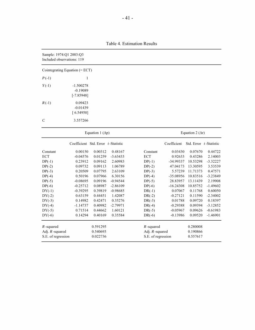
- 41 -

Sample: 1974:Q1 2003:Q3Included observations: 119

Cointegrating Equation (= ECT)

P (-1) 1

Y (-1) -1.500278-0.19089

[-7.85948]

R (-1) 0.09423-0.01439

[ 6.54950]

C 3.557266

Coefficient Std. Error t -Statistic Coefficient Std. Error t -Statistic

Constant 0.00150 0.00312 0.48167 Constant 0.03430 0.07670 0.44722ECT -0.04576 0.01259 -3.63433 ECT 0.92633 0.43286 2.14003DP(-1) 0.23912 0.09162 2.60983 DP(-1) -34.99337 10.53298 -3.32227DP(-2) 0.09732 0.09113 1.06789 DP(-2) 47.04173 13.30595 3.53539DP(-3) 0.20509 0.07795 2.63109 DP(-3) 5.57239 11.71373 0.47571DP(-4) 0.50196 0.07966 6.30156 DP(-4) -35.08956 10.83516 -3.23849DP(-5) -0.08695 0.09196 -0.94544 DP(-5) 28.83957 13.11439 2.19908DP(-6) -0.25712 0.08987 -2.86109 DP(-6) -16.24308 10.85752 -1.49602DY(-1) -0.39295 0.39819 -0.98685 DR(-1) 0.07067 0.11768 0.60050DY(-2) 0.63159 0.44451 1.42087 DR(-2) -0.27121 0.11590 -2.34002DY(-3) 0.14982 0.42471 0.35276 DR(-3) 0.01788 0.09720 0.18397DY(-4) -1.14737 0.40982 -2.79971 DR(-4) -0.29388 0.09394 -3.12852DY(-5) 0.71514 0.44662 1.60121 DR(-5) -0.05967 0.09626 -0.61983DY(-6) 0.14294 0.40169 0.35584 DR(-6) -0.13986 0.09520 -1.46901

R -squared 0.591295 R -squared 0.280008Adj. R -squared 0.540693 Adj. R -squared 0.190866S.E. of regression 0.022736 S.E. of regression 0.557617

Equation 1 (∆p) Equation 2 (∆r)

Table 4. Estimation Results

- 42 -

IV. BUDGETARY POLICYMAKING IN THE NETHERLANDS24

A. Introduction

62. Dutch fiscal policies are embedded in a medium-term expenditure framework. The framework has helped achieve considerable fiscal consolidation during 1994–2001. At the same time, it has allowed—to an increasing extent—the free play of automatic stabilizers. Although the framework offers no panacea for fiscal management issues and would benefit from some refinements, it has various desirable features and could possibly serve as a point of reference for other countries.

63. Another interesting feature of the Dutch fiscal policy setting is the role played by the Bureau for Economic Policy Analysis (CPB)—an independent agency that provides macroeconomic forecasts and policy analysis. The CPB is closely involved in the budgetary process. Importantly, it assesses in a highly visible and public manner consistency between the government’s policies and its fiscal and other economic objectives. Although the CPB does not explicitly set or actively enforce policy objectives, its analysis strongly influences perceptions of what constitutes “good policy.” Acting as an independent check on government policies, the CPB embodies some elements of the “independent fiscal councils” that have been advocated in the context of the European Stability and Growth Pact.25

64. The authorities have also recently introduced so-called performance budgeting, with a view to further strengthening the accountability of public sector spending. Here, the experiences have been mixed and highlighted several pitfalls with respect to the use of quantitative performance targets. Nonetheless, if managed judiciously, the clearer links between objectives, policy actions, and financing could further improve policymaking over time.

65. This chapter will describe and assess these key elements of fiscal policymaking in the Netherlands. It is organized as follows: First, Section B provides a brief overview of fiscal policy before the introduction of the current framework. Then, Section C discusses the medium-term expenditure framework and its track record. Section D addresses the role of the CPB, while Section E discusses the early experiences with performance-based budgeting. Section F concludes.

24 Prepared by David Hofman.

25 See, in particular, Annett (2004) and Annett and others (2005).

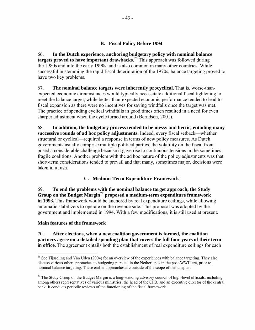
- 43 -

B. Fiscal Policy Before 1994

66. In the Dutch experience, anchoring budgetary policy with nominal balance targets proved to have important drawbacks.26 This approach was followed during the 1980s and into the early 1990s, and is also common in many other countries. While successful in stemming the rapid fiscal deterioration of the 1970s, balance targeting proved to have two key problems.

67. The nominal balance targets were inherently procyclical. That is, worse-than-expected economic circumstances would typically necessitate additional fiscal tightening to meet the balance target, while better-than-expected economic performance tended to lead to fiscal expansion as there were no incentives for saving windfalls once the target was met. The practice of spending cyclical windfalls in good times often resulted in a need for even sharper adjustment when the cycle turned around (Berndsen, 2001).

68. In addition, the budgetary process tended to be messy and hectic, entailing many successive rounds of ad hoc policy adjustments. Indeed, every fiscal setback—whether structural or cyclical—required a response in terms of new policy measures. As Dutch governments usually comprise multiple political parties, the volatility on the fiscal front posed a considerable challenge because it gave rise to continuous tensions in the sometimes fragile coalitions. Another problem with the ad hoc nature of the policy adjustments was that short-term considerations tended to prevail and that many, sometimes major, decisions were taken in a rush.

C. Medium-Term Expenditure Framework

69. To end the problems with the nominal balance target approach, the Study Group on the Budget Margin27 proposed a medium-term expenditure framework in 1993. This framework would be anchored by real expenditure ceilings, while allowing automatic stabilizers to operate on the revenue side. This proposal was adopted by the government and implemented in 1994. With a few modifications, it is still used at present.

Main features of the framework

70. After elections, when a new coalition government is formed, the coalition partners agree on a detailed spending plan that covers the full four years of their term in office. The agreement entails both the establishment of real expenditure ceilings for each 26 See Tijsseling and Van Uden (2004) for an overview of the experiences with balance targeting. They also discuss various other approaches to budgeting pursued in the Netherlands in the post-WWII era, prior to nominal balance targeting. These earlier approaches are outside of the scope of this chapter.

27 The Study Group on the Budget Margin is a long-standing advisory council of high-level officials, including among others representatives of various ministries, the head of the CPB, and an executive director of the central bank. It conducts periodic reviews of the functioning of the fiscal framework.

- 44 -

of the four years, as well as a comprehensive package of policy measures needed to deliver adherence to the ceilings. The various choices involved are extensively negotiated and laid down in a detailed “Coalition Agreement,” which subsequently serves as the basis for policy making during the government’s term. A key advantage of this approach is that it effectively puts all the big decisions up front, thereby reducing the potential for discord between the coalition partners along the way.

71. The levels of the real spending ceilings and the associated policy measures are based on the prospective government’s assessment of the needed fiscal adjustment during the government period. That is, at the time the spending ceilings are negotiated, they imply a specified path of fiscal adjustment for the government term, given certain assumptions regarding the macroeconomic outlook, potential growth, and the estimate of the fiscal balance in the base year (which, of course, may later be revised). The amount of effort implied in the four-year plan is a political decision, guided by various considerations including analyses of the fiscal challenges of population aging and the requirements in the context of the Economic and Monetary Union (EMU) and the accompanying Stability and Growth Pact (SGP).28

72. Once the coalition agreement is concluded and the real expenditure ceilings are set, the level of expenditure serves as the policy target. The fiscal balance is allowed to fluctuate freely with developments in revenues. In contrast to the practice before 1994, there is a strict separation between revenues and expenditures. When revenue setbacks—which are often related to weaker-than-expected economic growth—cause a deterioration of the fiscal balance, no adjustment measures are required. Likewise, higher-than-expected revenues are also fully reflected in the balance and cannot be used for additional spending. The framework thus allows for the free play of automatic stabilizers on the revenue side. This play is limited only by the requirements of the SGP: the fiscal rules stipulate that if during the government’s term actual developments in revenues disappoint up to the point that the deficit is expected to exceed 2.5 percent of GDP, additional measures need to be taken in order to prevent a breach of the 3 percent of GDP Maastricht deficit ceiling.29 It should be noted that in earlier years, the framework was less binding in the sense that the partial use of revenue windfalls to finance tax cuts was permitted, with the degree depending on overall fiscal performance. However, the use of revenue windfalls for this purpose was ended in 2002.

28 For example, during 1994–98, when the Netherlands had to secure compliance with the deficit and debt criteria of the Maastricht Treaty in order to qualify for EMU membership, the ceilings were set to decline by 0.7 percent every year, implying rapid consolidation. In the subsequent period (1998–2002), with the public finances in a better shape, the effort was relaxed, allowing real spending growth of 1.5 percent per year—which still implied considerable adjustment in light of an average real GDP growth of 2.8 percent (ex post) during that period. In the current government’s term (2004–07), ceilings were set to increase by 1.4 percent a year in real terms, originally implying a nominal deficit of 0.5 percent of GDP in 2007, which was deemed consistent with a sustainable path for public finances, while providing for population aging.

29 The 2.5 percent threshold represents the desire to maintain a 0.5 percent safety margin with respect to the Maastricht ceiling.

- 45 -

73. Another distinctive feature of the framework is a conservative approach to budgeting. In deciding on its four-year spending plan, the government uses “cautious” assumptions with respect to the macroeconomic outlook, relying on a conservative growth scenario supplied by the CPB. The implication of this approach is that any surprises during the budget execution are likely to be on the upside. This would seem prudent as it is harder to compensate for setbacks than it is to allocate windfalls. In addition, since the emphasis, at least for the foreseeable future, is on fiscal consolidation, it makes sense to err on the side of larger-than-planned adjustment.

74. The overall spending ceilings are subdivided into subceilings for three separate sectors. These are (i) a “core” sector; (ii) social security; and (iii) the health care sector. Subsequently, these subceilings are translated into specific budgets for each individual ministry. In principle, every minister is responsible for meeting the budget ceiling of his/her ministry. There are specific rules that deal with the use of windfalls. Within its own budget, each ministry is allowed to use expenditure windfalls that may occur during the year to compensate for expenditure setbacks. However, expenditure windfalls may not be used to fund new spending without further consideration by the cabinet. The latter rule was added in 2002 in order to prevent a repetition of the experiences of the 1990s when, with hindsight, cyclical expenditure windfalls had been used to finance new structural spending. Compensation may also occur between ministries, but not across the three main government sectors.30 Revenue windfalls, as mentioned above, are to be saved under all circumstances.

Specifics of the expenditure ceilings

75. In the four-year plan, the ceilings are set in real rather than nominal terms. This facilitates compatibility with the associated policy measures and makes the plans robust with respect to unexpected price developments, thereby fostering political tranquility. However, actual expenditure is, of course, in nominal terms. Therefore, every year, in the budget memorandum, the real ceilings for that year are translated into operational nominal ceilings on the basis of expected price developments.31 In the Spring, when the budget for the current year is updated, the deflator forecast is reviewed and the ceilings are adjusted accordingly. After the Spring review, the ceilings for the current year remain fixed in nominal terms.

76. The coverage of the expenditure ceilings is wide, but not exhaustive. In a typical year, around 85 percent of public expenditures will be subject to the ceilings (Figure 1). Interestingly, and somewhat at odds with the countercyclical qualities of other elements of the framework, unemployment spending is included under the ceilings. But other, noncyclical, spending is excluded. The two main excluded items are expenditures from a special fund for investment in infrastructure and the spending of local governments. 30 The rule that bans compensation across the three main sectors has not always been adhered to in the past, but the current government renewed its commitment to the rule when it took office.

31 Specifically, a forecast for the domestic demand deflator is used for this purpose.

- 46 -

Figure 1. Netherlands: Expenditure Development, 1999-2003(In percent of GDP)

Sources: Ministry of Finance, CBS, and IMF staff estimates.

0

10

20

30

40

50

60

1999 2000 2001 2002 2003

Expenditure according to national accounts (ESA 95 basis)Expenditure subject to the ceiling

77. The infrastructure fund is funded with revenues from natural gas sales and interest savings resulting from the sale of government properties.32,33 The fund has been separated from the budget process in order to exclude these volatile revenue sources from the general budget and to safeguard a sufficiently high level of infrastructure investments, which improve the economic structure. While there may be advantages to this arrangement from a political economy perspective, the earmarking has the disadvantage of separating the infrastructure investments from the trade-offs faced in the general budgetary process and of reducing the reach of the expenditure ceilings.

78. While local government spending is subject to the requirement that budgets must be balanced over the medium term, problems may arise because local governments’ accounts are compiled on a different basis than those of the central (and general) government. In particular, the local governments are allowed to spread out the fiscal impact of large investments over time by booking the annual depreciation rather than the full amount of the investment. This enables local governments to undertake relatively large investments, without breaching the medium-term balance requirement. However, in the consolidated general government accounts on an ESA 95 basis, such investments have to be booked up front, so that the actions of the local governments can pose problems for the general government’s balance in EMU-consistent terms. Further risks stem from the local

32 Investments from the infrastructure fund pertain, for example, to highways and high speed rail connections.

33 The proceeds of the sale of government properties are used to pay down government debt. The resulting structural flow of savings on the interest bill is then deposited in the infrastructure investment fund.

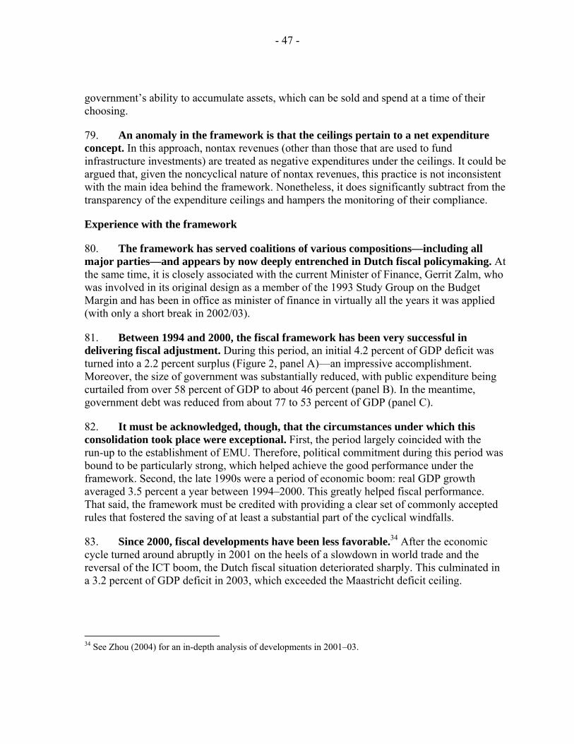
- 47 -

government’s ability to accumulate assets, which can be sold and spend at a time of their choosing.

79. An anomaly in the framework is that the ceilings pertain to a net expenditure concept. In this approach, nontax revenues (other than those that are used to fund infrastructure investments) are treated as negative expenditures under the ceilings. It could be argued that, given the noncyclical nature of nontax revenues, this practice is not inconsistent with the main idea behind the framework. Nonetheless, it does significantly subtract from the transparency of the expenditure ceilings and hampers the monitoring of their compliance.

Experience with the framework

80. The framework has served coalitions of various compositions—including all major parties—and appears by now deeply entrenched in Dutch fiscal policymaking. At the same time, it is closely associated with the current Minister of Finance, Gerrit Zalm, who was involved in its original design as a member of the 1993 Study Group on the Budget Margin and has been in office as minister of finance in virtually all the years it was applied (with only a short break in 2002/03).

81. Between 1994 and 2000, the fiscal framework has been very successful in delivering fiscal adjustment. During this period, an initial 4.2 percent of GDP deficit was turned into a 2.2 percent surplus (Figure 2, panel A)—an impressive accomplishment. Moreover, the size of government was substantially reduced, with public expenditure being curtailed from over 58 percent of GDP to about 46 percent (panel B). In the meantime, government debt was reduced from about 77 to 53 percent of GDP (panel C).

82. It must be acknowledged, though, that the circumstances under which this consolidation took place were exceptional. First, the period largely coincided with the run-up to the establishment of EMU. Therefore, political commitment during this period was bound to be particularly strong, which helped achieve the good performance under the framework. Second, the late 1990s were a period of economic boom: real GDP growth averaged 3.5 percent a year between 1994–2000. This greatly helped fiscal performance. That said, the framework must be credited with providing a clear set of commonly accepted rules that fostered the saving of at least a substantial part of the cyclical windfalls.

83. Since 2000, fiscal developments have been less favorable.34 After the economic cycle turned around abruptly in 2001 on the heels of a slowdown in world trade and the reversal of the ICT boom, the Dutch fiscal situation deteriorated sharply. This culminated in a 3.2 percent of GDP deficit in 2003, which exceeded the Maastricht deficit ceiling.

34 See Zhou (2004) for an in-depth analysis of developments in 2001–03.

- 48 -

Figure 2. Netherlands: Trends in Public Finances, 1970-2004(In percent of GDP)

Sources: CPB; and IMF staff calculations.

A. Fiscal Balance of the General Government

-7

-6

-5

-4

-3

-2

-1

0

1

2

3

1970 1972 1974 1976 1978 1980 1982 1984 1986 1988 1990 1992 1994 1996 1998 2000 2002 2004

B. Expenditures and Revenues of the General Government

35

40

45

50

55

60

65

70

1970 1972 1974 1976 1978 1980 1982 1984 1986 1988 1990 1992 1994 1996 1998 2000 2002 2004

Expenditures

Revenues

C. Government Debt

20

30

40

50

60

70

80

90

1970 1972 1974 1976 1978 1980 1982 1984 1986 1988 1990 1992 1994 1996 1998 2000 2002 2004

- 49 -

84. The sharp deterioration of the balance took the authorities—as well as most outside observers—by surprise. Nevertheless, even though there are indications that, during the boom years, cyclical expenditure windfalls had been used to finance new structural expenditures, on balance, there was no sizable fiscal slippage vis-à-vis the spending ceilings that were set. Indeed, the ceilings were generally adhered to (see e.g., Reininga (2001) and Zhou (2004)). The only overruns occurred in 1998 and in 2003 and were minimal (€200 and €400 million, respectively, or less than 0.1 percent of GDP in both cases).

85. The deterioration during 2001–03 mainly reflected three factors:

• Relative stance of expenditure policy. The levels of spending for 2001, 2002, and 2003 had been determined at a time when the outlook—even on “cautious” assumptions—was considerably more favorable than the actual outturn. By implication, even with the ceilings adhered to, the pre-set spending policies turned out much more expansionary than originally envisaged, in the sense that expenditure grew relatively rapidly in comparison to real GDP. To illustrate, when the ceiling for 2003 was set in the coalition agreement of the Summer of 2002, it was assumed that real GDP would grow by 2.5 percent in 2003. The outturn, however, was a 0.9 percent decline of GDP. The forecasting error for 2003 alone accounted for about 1¼ percentage points of the deterioration of the fiscal balance in comparison to the projected baseline.

• Cyclicality of revenues and tax reductions. Another part of the fiscal worsening since 2000 was due to developments in taxes. Tax revenues and social security contributions declined from 40.6 percent of GDP in 2000 to 38.7 percent in 2003, explaining almost 2 percentage points of the deterioration in the balance. Part of this was the likely reflection of the fact that, under the then prevailing rules for the allocation of revenue windfalls, cyclical windfalls had been used to finance permanent tax cuts. In particular, some 0.8 percentage point of the fall in the revenue ratio was related to the tax cuts in 2001, which, with the benefit of hindsight, had been based on an overly sanguine assessment of the structural revenue position. Indeed, wealth effects amplified the normal cycle, causing large revenue gains during the upswing, which were initially regarded as structural but later turned out to be cyclical, partly reflecting tax elasticities having apparently changed over the cycle.

• Increases in spending not subject to ceilings. In 2003, after running close to balance for many years, the local governments unexpectedly ran a 0.6 percent of GDP deficit on account of spending financed by the sale of earlier accumulated assets. The surprise overrun on the part of the local governments contributed to the general government balance breaching the 3 percent of GDP Maastricht deficit ceiling.

86. These factors highlight that the operation of the framework critically hinges on the quality of the macroeconomic projections. To the extent that the sharp deterioration is explained by the relative stance of expenditure policy and the cyclical volatility of revenues,

- 50 -

losses should eventually come back during the next upswing. Crucially, however, this only holds to the extent that the underlying assumptions with respect to the potential growth rate have been accurate. While the practice of fixing expenditure levels for four years ahead has clear advantages in terms of precommitment and helps prevent the spending of revenue windfalls in good times, it has a potential downside, too. If the estimate of potential growth turns out to be too high, the government will have, unknowingly, committed itself to a more expansionary policy stance for multiple years than would seem to have been intended. Although definitive conclusions can only be drawn ex post, this may be a relevant issue at present.

87. Apart from this fundamental conceptual issue, the recent experience also highlights a few other areas where the application of the framework has had shortcomings. Clearly, cutting taxes in the presence of sizable revenue windfalls and the associated difficulties involved in distinguishing between cyclical and structural components had its drawbacks. It is therefore welcome that the authorities have discontinued the practice of using revenue windfalls to finance cuts in taxes. Also, the strong cyclical volatility of revenues needs to be taken into account. Specifically, when fiscal consolidation is important, this would seem to argue for building, and then maintaining, a fiscal buffer as an insurance policy against unexpected sharp cyclical swings in revenues. A final lesson is that the exclusion of relevant expenditure items from the framework further reduces assurances about fiscal outcomes, thus posing a risk to adherence to the SGP. Therefore, such items could be usefully included through a widening of the coverage of the ceilings or through other measures with similar effect. In this regard, the authorities’ recent trial with an “internal stability pact” that aims at closely coordinating the fiscal policies of the central and local governments, is encouraging.

88. Since 2003, the government has taken far-reaching measures to redress the fiscal worsening. Consistent with the provision in the framework that additional measures are called for in case compliance with the SGP is threatened, the government implemented a host of new measures in 2004, aimed at bringing the deficit back under the 3 percent Maastricht ceiling. In the event, it accomplished structural adjustment of about 1¼ percentage points of GDP, reducing the deficit to 2.3 percent of GDP. In a sense, the emergency measures constituted a temporary return to balance targeting.

D. Role of the CPB

89. The CPB, or Netherlands Bureau for Economic Policy Analysis was established in 1945 as the “Central Planning Bureau” and plays a central role in the political process and policy making in the Netherlands. While it was originally intended to facilitate the central coordination of government policies and to provide advise on the sectoral production plans in the private sector (hence the socialist flavor in the initial naming of the institution), the agency has over time assumed a very different role—that of an independent economic forecaster and evaluator of public sector policies. In the latter capacity, the CPB does not provide direct policy recommendations. Rather, it tends to take an “academic” approach, stating facts and pointing out the expected effects of different courses

- 51 -

of action, but refraining from normative judgments. Testimony to its apparent success in maintaining this impartial role, the CPB is widely accepted and respected—by political parties and the public at large—as an independent and credible source of economic projections and policy analysis.

Independence

90. While a government body (it is technically under the ministry of economic affairs), the CPB enjoys complete operational freedom, formally guaranteed by law. The director is appointed by the government, but in practice, the process appears to be relatively nonpolitical. CPB directors typically outlive various governments, irrespective of their personal party affiliation. The independence of the CPB management is rarely, if ever, questioned.

Role of the CPB in the political and budgetary process

91. The CPB plays a key role at various stages in the political process. Prior to elections, the CPB provides comprehensive medium-term macro forecasts that are used by the political parties as the basis for their policy platforms. In addition, the larger parties voluntarily submit their platforms to the CPB for an assessment of their economic impact. They do so mainly because a favorable CPB assessment greatly enhances the credibility of their proposals, and also because reluctance to submit to the scrutiny of the CPB would signal that their proposals are not sound. CPB assessments help to track errors and inconsistencies in the platforms, and political parties use the CPB’s expertise to help shape their proposals with a view to optimizing the expected economic effects (depending on political preferences, of course). In effect, the CPB provides the political parties with something of a level playing field in terms of economic forecasts and in the methodology by which policy proposals are evaluated. As a result, unlike their counterparts in many other countries, Dutch political parties generally do not quarrel about differences in macroeconomic assumptions or the expected economic impact of proposed measures.

92. After elections, the CPB plays an important role in assisting in the formation of a new coalition government. It provides an updated set of medium-term projections that forms the basis for the coalition agreement and the medium-term expenditure plan included in it. Often, the CPB is asked to supply a number of different growth scenarios from which the coalition partners choose their baseline (as discussed above, they traditionally opt for the most “cautious” scenario). Subsequently, the CPB works with the prospective coalition partners on the design of a consistent coalition agreement, a process greatly facilitated by its role in the prior assessment of the individual party platforms (i.e., by the time of the coalition negotiations, the economic features of the various policy proposals are known). In terms of the design of the medium-term fiscal framework, the CPB provides several of the key inputs such as the macroeconomic assumptions and the estimate of potential growth. It does not, however, set any fiscal targets—that is the prerogative of the government, with the CPB only assessing consistency between the proposed policies and the expected fiscal outcomes.

- 52 -

93. Once in office, the government continues to use the macroeconomic projections of the CPB. Specifically, CPB forecasts are used as the basis for the government’s annual budgets (including, for example, forecasts of the deflator that is used to translate the real spending ceilings of the medium-term framework into operational nominal targets for the current budget year), the Stability Program updates, and the projections of fiscal outcomes. The government does not make, or publish, any macroeconomic projections of its own. The provision of independent forecasts by the CPB serves a critical role in the elimination of possible politically-motivated forecast biases—a point that has also been emphasized in recent literature (see e.g., Jonung and Larch (2004)). Of course, the absence of political biases—however important—does not guarantee that CPB projections are always right, as has been amply highlighted by the recent experience described above.

94. Besides the regular involvement in the budgetary process, the CPB also provides ad hoc analyses of key economic issues. It does so both on its own initiative and in response to specific requests from the government or parliament. Topics covered include, for example, the fiscal cost of aging and the effects of the regulatory environment on economic growth. The CPB also regularly analyzes (aspects of) new policy proposals, such as, for instance, the overhaul of the disability scheme and health care reform.

Accountability of the CPB

95. While the CPB is a very influential institution, given its central role in the policy process and virtual monopoly position, there are forces to keep it in check. Clearly, the CPB can function effectively only by virtue of its reputation for impartiality and sound economic reasoning, and much of what the CPB does is published and under continuous public and academic scrutiny. In addition, the performance of the CPB is regularly assessed by outsiders: for example, in 2001, its role in the field of policy formation was reviewed by an ad hoc committee of domestic officials; and in 2003, it was assessed by an international independent scientific review committee.

The CPB and Independent Fiscal Councils

96. Against the background of the recent amendments to the SGP, a case has been made for strengthening national fiscal institutions in EMU member states, in particular through the establishment of so-called Independent Fiscal Councils (IFCs) (Annett (2004) and Annett and others (2005)). An IFC would be a national watchdog body providing independent assessments of fiscal policies and monitoring compliance with the SGP. If the IFC is sufficiently credible, its highlighting of any deviations by the government from either the budget or the stability program could lead to reputational costs for the government, thereby acting as a disciplinary device.

97. In practice, the role of the CPB is similar to that of an IFC. In particular, the CPB clearly provides an independent check and, given its great credibility, has the power to bring reputational costs on the government. A key difference, however, with the IFCs that have recently been advocated is that the role of the CPB is not in any way linked to the EMU

- 53 -

requirements or the SGP. The CPB makes its own assessments of fiscal policy needs, independent of the European Commission, and does not regard itself as a guardian of Dutch SGP compliance. That said, in recent periods, such a reference to the SGP has not been necessary as the Dutch government itself has been strongly committed to compliance with European rules.

E. Performance Budgeting

98. Starting with the 2002 budget, the authorities have introduced a system of so-called “performance budgeting.” The general idea behind this approach—which is increasingly applied, to varying degrees, in many other OECD countries—is to enhance the transparency of the budget and government policies, with a view to improving accountability. To this end, budgets explicitly link (i) the ultimate policy goals; (ii) the associated policy actions; and (iii) the available financing. More specifically, to facilitate accountability, quantitative performance targets are set for the ultimate policy goals as well as for various throughput variables. After a fiscal year has ended, every ministry is required to submit an annual report that discusses the effectiveness of policies and the extent to which policy goals have been met, with reference to the quantitative targets.35

99. The experience with performance budgeting in the Netherlands has thus far been mixed.36 On the upside, the transparency of budget memoranda and their accessibility to a wider audience appear to have been enhanced considerably. In addition, improved prioritization has led to a drastic reduction in the overall number of spending items, thus contributing to the manageability of public policy. However, the new approach is also experiencing significant growing pains.

100. A key issue is the identification of meaningful performance indicators. In many instances, the way in which the effects of government policies should be measured is not straightforward, and measurement problems hamper accountability in various areas. In the four years that performance budgeting has been applied, the government succeeded in covering only about half of all policies with measurable quantitative targets. In addition, concerns have been raised about the adequacy of many of these targets. Inevitably, performance targets measure only one, or at best a few, dimensions of policy effectiveness,

35 For example, in the area of crime, the government’s ultimate policy objective is to reduce crime rates by 20-25 percent between 2002 and 2010. To achieve this goal, it pursues a policy of increasing, among various other things, the size of the police force and the capacity of penitentiary institutions. For the latter operational variables, quantitative targets are set in each year’s budget, together with the funding available to achieve them. In its annual reports, the government discusses to which extent the intermediate targets (more police, more prison cells) have been met, the amounts of tax money spent, and the progress made towards the overall objective (less crime).

36 The early experiences with performance budgeting were reviewed in 2004 by an interministerial working group (IOFEZ, 2004). The discussion in this section draws on their findings as well as on those of Tijsseling and Van Uden (2004).

- 54 -

thereby risking an oversimplification of sometimes complex issues. Moreover, since nobody in the public sector has an interest in documenting failure, there is a risk that in practice, the most easily attainable targets are selected, rather than the most relevant ones.

101. Another main drawback is the bureaucracy and extensive paperwork that has so far been associated with the measurement and accountability process. The combined policy evaluations and annual reports that are written by each ministry reportedly span several thousands of pages each year. This places a considerable burden on the reporting ministries, and there have been complaints that the average quality of evaluations is below par. Against this background, on the other end of the spectrum, parliamentarians have so far shown little appetite for digesting the plethora of reports, and the annual discussions on past policy performance in parliament have been mostly uneventful.

102. Further problems pertain to managing trade-offs in areas where policies of different ministries affect each others success, and to the difficulties in accounting for exogenous factors—outside of the control of the government—that may influence policy outcomes. Also, the incentive structures faced by public sector managers have not yet been adjusted to the accountability framework, so that neither success nor failure to meet a target has direct consequences for the managers involved.

103. These issues argue for moving ahead gradually and selectively. Most of the problems are not unique to the Netherlands and are also experienced in other countries that have experimented with performance evaluation (see e.g., IMF, 2005). While there may be no easy answers to the problems, the overall goal of improving accountability remains a legitimate and important one. It would seem recommendable, however, to take a step-by-step approach to implementing performance budgeting. This would involve focusing first on policy areas where measurement is relatively straightforward and quantitative targets make most sense, then expanding only gradually to more complex areas, recognizing that a comprehensive coverage of policies may not be attainable for some time to come.

F. Summary and Conclusions

104. The Dutch budgetary framework has considerable merits. Its medium-term focus allows for multi-year commitment by the government, thereby lessening the role of (often political) short-run considerations, and putting a premium on structural policy measures. At the same time, by targeting real expenditure, while allowing automatic stabilizers to play freely on the revenue side, it normally avoids procyclical policy biases.

105. A main practical challenge for the framework concerns the accuracy of the four-year macroeconomic projections, including the underlying estimate of potential growth. If the potential growth rate is overestimated, this can, in effect, result in a commitment to overly expansionary fiscal policies. While the conservative budgeting approach that has been applied by the government helps alleviate this problem, the recent experience has shown that risks remain, especially at times when there is greater-than-usual uncertainty about the economic outlook.

- 55 -

106. Some refinements could improve fiscal policies under the framework. In light of the recent experiences that revealed strong cyclical components in revenues, a cautious approach to ensuring adequate funding for any further tax cuts would seem appropriate, as would building and maintaining a fiscal buffer to safeguard consolidation objectives and SGP compliance from unexpected swings in revenues. In addition, in order to improve the predictability of fiscal outcomes, the coverage of the framework could be usefully extended to integrate items—such as local government spending—that are currently excluded. Finally, focusing the spending ceilings exclusively on spending by ending the practice of treating nontax revenues as negative expenditures, would enhance transparency.

107. The CPB plays a key role in keeping fiscal discipline. By publicly assessing consistency between the government’s policy measures and its fiscal and other economic objectives, the CPB fosters accountability and fiscal discipline. In various respects, the CPB is a successful example of an “Independent Fiscal Council,” although it does not explicitly prescribe fiscal targets or policy measures and has no particular interest in Dutch SGP compliance.

108. The experiences in the area of performance budgeting argue for moving ahead in small steps. While performance budgeting raises the prospect of improved efficiency and accountability of fiscal policy, its implementation is somewhat of a “trial-and-error” process. In this light, efforts should focus on policy areas where quantitative targets make most sense, expanding only gradually into more complex areas.

- 56 -

REFERENCES

Annett, Anthony, Jörg Decressin, and Michael Deppler, 2005, “Reforming the Stability and Growth Pact,” IMF Policy Discussion Paper, PDP/05/2 (Washington: International Monetary Fund).

Annett, Anthony, 2004, “Enforcement and the Stability and Growth Pact,” in IMF Staff Country Report 04/235 (Washington: International Monetary Fund).

Blöndal, Jón, and Jens Kromann Kristensen, 2002, “Budgeting in the Netherlands,” OECD Journal on Budgeting, Vol. 1, No. 3, pp. 39–77.

Berndsen, Ron, 2001, “Postwar Fiscal Rules in the Netherlands: What Can We Learn for EMU?,” in Fiscal Rules, Proceedings of a BdI Workshop (Rome: Banca d’Italia).

IOFEZ, 2004, “Policy Budgets and Policy Accountability: Evaluation—Lessons from Practice” (The Hague: Ministry of Finance).

IMF, 2005, “United Kingdom: Staff Report for the 2004 Article IV Consultation,” Country Report No. 05/80 (Washington: International Monetary Fund).

Jonung, Lars, and Martin Larch, 2004, “Improving Fiscal Policy in the EU: the Case for Independent Forecasts,” European Economy Economics Papers No. 210 (Brussels: European Commission).

Reininga, Ted, 2001, “Coalition Governments and Fiscal Policy in the Netherlands,” in Fiscal Rules, Proceedings of a BdI Workshop (Rome: Banca d’Italia).

Tijsseling, I.C., and P.G.J. Uden (eds.), 2004, “Made in Holland—Dutch Public Finance: Lessons and Experiences” (The Hague: Sdu Publishers).

Zhou, Jianping, 2004, “Recent Fiscal Developments in the Netherlands,” in IMF Country Report No. 04/301 (Washington: International Monetary Fund).

- 57 -

V. THE FINANCIAL SECTOR IN THE NETHERLANDS: A HEALTH CHECK AND PROGRESS REPORT ON THE FSSA RECOMMENDATIONS37

109. Following up on the 2004 Financial System Stability Assessment (FSSA), this paper has two purposes. The first is to review recent developments in the financial sector since the FSSA was completed last year. The second is to discuss the progress made on the recommendations from the FSSA. As noted in the staff report for the 2005 Article IV Consultation, staff found no reason to depart from the main conclusion of the FSSA—namely that the Dutch financial system is sound, resilient to potential adverse shocks, and well supervised.38

A. Recent Developments

110. Little has changed in the structure of the financial system since the publication of the FSSA (Table 1). There were minor changes in the number of banks and insurance companies. The downward trend in the number of pension funds continued as the sector consolidated in pursuit of further efficiency gains.

111. Banks improved their balance sheets and their profitability in 2004. The capital-to-asset ratio of deposit-taking institutions continued to increase, and the ratio of their trading income to total income followed a cyclical recovery (Table 2). Meanwhile, despite the flattening of the yield curve and a related reduction in banks’ margins, returns on both assets and equity increased as the volume of transactions rose and banks continued their effort to reduce costs (Table 3). Traditionally ample liquidity in Dutch banks increased further. With respect to financial derivatives, the pick-up in activity reflected market developments: credit default swaps and collateralized debt obligations (known as CDSs and CDOs in market jargon) have expanded exponentially on a global basis, and developments in the Dutch market followed this trend. The increase in loans to other financial institutions reflected a rise in interbank lending, which is typical during this phase of the cyclical upswing.

112. While house price growth moderated in 2004, mortgage lending continued to rise. This partly reflected growth in refinancing, with the market apparently holding the view that the trough in the current interest rate cycle had been reached. Loan-to-value (LTVs) ratios in recent times have been high for new loans, averaging about 105 percent (though the average for all loans is considerably lower).39 Activity was largely confined to the highly 37 Prepared by Francisco Nadal De Simone.

38 The Kingdom of the Netherlands—Netherlands: Financial System Stability Assessment, including Reports on the Observance of Standards and Codes on the following topics: Banking Supervision, Securities Regulation, Insurance Regulation, Corporate Governance, and Payments Systems, Securities Settlement Systems, and Anti-Money Laundering/Combating the Financing of Terrorism, IMF Country Report N. 04/312, September 2004.

39 LTV ratios are not regulated in the Netherlands. Regulations apply to the ability to pay rather than to the ability to reclaim value (i.e., income-to-value ratio as opposed to LTV). Moreover, the tax deductibility of mortgage interest payments has been factored into loan demand. Finally, it is also possible that the increased

(continued)

- 58 -

competitive banking sector (insurance firms and other financial institutions are also allowed to sell mortgages), with banks continuing to reduce their margins and offering interest-free initial mortgage periods.40

113. The performance of the insurance sector also improved in 2004. While a low interest rate environment continued to limit the returns of life insurance providers, both parts of the insurance sector improved their profitability, helped by better stock market performance, and with nonlife providers also benefiting from further reductions of costs and limits on claims. However, if the low interest rate environment were protracted, it may lead to concerns over firms’ solvency in the future.41 Because it operates on a low duration gap, these concerns are much less pertinent to the nonlife sector, as short duration liabilities make it easier to better match assets and liabilities.

114. Pension fund returns edged down in 2004—though they still remained high and the funds boosted their asset-liability (or coverage) ratio (Table 4). Although interest rates were low, pension funds benefited from higher equity prices and a shift in the composition of their portfolios to equities. Pension funds also increased contribution rates, and this contributed to the rise in their asset-liability ratio to 124 percent.42

115. The debt of households continued to move higher in 2004, albeit at a much slower rate than in previous years. The authorities indicated that nonperforming loans (NPLs) of households doubled (according to preliminary data), though from a very low base.

116. The liquidity and profitability in the corporate sector improved in 2004. Corporations reduced their debts at the same time that profitability rose. Meanwhile, firms also refinanced loans at lower interest rates. Consistent with the pickup in corporate profitability, the authorities indicated that NPLs of the corporate sector declined.

117. On the financial policy front, the Dutch integrated supervision scheme has already produced a number of benefits, both from a policy perspective and operationally. From a policy viewpoint, teams working on Basel II and Solvency II could

share of mortgages in banks’ portfolios observed in several countries reflects markets’ anticipation that Basel II will reduce capital requirement on mortgage lending.

40 A concern related to the mortgage market is the growing take-up in interest-only mortgages and the difficulty in tracking and assessing the risk related to the investment of associated funds to cover the future payment of principal.

41 The life sector is still recovering from the reduction in returns after the removal of tax deductibility of life insurance premia in 2001.

42 As discussed below, the solvency ratio starting in 2006 will be determined on the basis of market interest rates instead of a fixed discount rate as used now. Market rates would imply a decline in the solvency ratio from 129 percent in 2003 to 123 percent in 2004.

- 59 -

beneficially be combined, and this has resulted in cross-group information and expertise-sharing.43 At an operational level, benefits have also been significant, particularly for supervision of large and complex financial institutions in the Netherlands, which are the critical components of the sector. Integration has also allowed for the institutional transfer of human capital and the use of risk assessment tools drawing on the best approaches adopted when supervising banks, pension funds, and insurance firms separately.

118. Reflecting the move toward integrated supervision, financial crisis management and planning have been restructured within the Netherlands’ central bank (DNB). The DNB has identified a crisis team that can become operational on short notice, and strengthened support for this team in order to further improve the DNB’s crisis preparedness. Plans have not been tested internally yet, although the DNB has participated in a euro system stress test and will also likely take part in another multinational financial sector crisis management “war game” foreseen for Spring 2006.

119. A new Financial Supervision Act is expected to become law on January 1, 2006. The new law (some key details of which are discussed in Section B below) is intended to be “super neutral”—i.e., implementing all EU legislation, while also incorporating additional national measures exceeding or extending EU minima.44

120. Key institutional changes to pension funds will also be introduced on January 1, 2006. Three main areas involved are: (i) solvency or coverage requirements;45 (ii) the introduction of “fair value accounting”, which will ensure that pension funds mark to market their assets and liabilities frequently; and (iii) increased transparency for beneficiaries over their anticipated payouts. With respect to the latter change, it is important that second tier pensions in the Netherlands are defined-benefit plans. While most funds attempt to provide full indexation, they do not guarantee it and they have had the flexibility to provide only partial indexation in years when returns are poor or assets are being built up. The new regulatory regime will ensure that nominal benefits, at a minimum, are guaranteed, and that pension funds are clear and explicit about the extent to which indexation is being guaranteed. In addition, higher coverage ratios will be required as the level of guaranteed indexation increases. All this implies that the average coverage ratio will need to be increased from its current level.

43 As Solvency I is not considered sufficiently risk based by the authorities, they are working to influence and accelerate the development and introduction of Solvency II within the context of the Insurance Committee of the European Commission.

44 At the same time, the authorities are striving to reduce the administrative burden on firms, an objective that also is taken into account in designing financial policy. Against this background, the authorities did not include in the Act, as suggested by the FSSA, audit committees for individual banks.

45 Coverage requirements—expressed in terms of the coverage ratio, which is defined as the ratio of the present value of assets over liabilities—depend on the risk profile of the individual pension fund’s investment portfolio and the degree of guaranteed indexation of benefits.

- 60 -

121. New legal requirements to increase pension fund coverage ratios could have macroeconomic consequences. In cases where full indexation is not guaranteed, the minimum requirements imply a coverage ratio, on average, of 130 percent, compared with the coverage ratio of 124 percent at end-2004. When the coverage ratio is lower than 130 percent, it needs to be restored, as agreed with the supervisor, within a period not exceeding 15 years (at end-2004, Dutch pension funds held roughly €505 billion in assets). Increasing the coverage ratio, depending on how it is spread out, could affect contributions in a way that affects savings and therefore consumption behavior, and the macro economy. At the same time, the new regulatory framework could lead to changes in the pension funds’ asset allocations. Hypothetically, for example, pension funds could pursue a more risk-averse investment strategy, shifting away from equities to bonds. Given that reduced returns over the long run could also have a macroeconomic impact, the potential implications of the new requirements will need careful monitoring.

B. FSSA Recommendations

122. This section elaborates on the actions taken with regard to the FSSA recommendations summarized in Box 2 of the Staff Report. It is organized by recommendation and draws heavily on material provided by the authorities.

123. Recommendation I: Spell out clearly the role of the minister of finance, as applicable, in those few areas where autonomy is not fully delegated to the supervisor.

Starting in 2004, the approval of the minister of finance has only been needed if one of the five largest banks or insurers takes a participation in each other. The requirement in those cases follows from the minister’s political accountability for the well-functioning of the financial system and the budgetary consequences of a potential systemic crisis. In the new Supervisory Act mentioned above, this task will be delegated to the supervisors directly by law, with the licensing of financial institutions done solely by the supervisory authorities.

124. Recommendation II: Ensure that the Authority for Financial Markets (AFM) has the power to cooperate with securities supervisors internationally even when there is no “domestic interest.”

Cooperation of the AFM with supervisory authorities in other Member States is part of the new Financial Supervision Act. For non-Member States, the Act stipulates that under certain conditions, information exchange may take place (this is not compulsory).

125. Recommendation III: Continue to work with cross-border counterparts to further improve securities settlement arrangements.

- 61 -

Improvements are being made through supporting Euroclear's single settlement platform and promoting the use of delivery of securities against payment (DVP) in making settlements. However, DVP will not be used in all cases and there will always be some free of payments transactions (FOP). The AFM and the DNB have approved a proposal from Euroclear Netherlands to admit investment firms as participants, and they actively support the Euroclear initiative for building a Single Settlement Engine/Single Application Platform for cross-border DVP in 2007. While the first three parts of the new Financial Supervision Act come into effect at the start of 2006, the fourth part on market infrastructure is expected to be finalized by July 2006.

126. Recommendation IV: Ensure that the new pensions supervisory arrangements allow sufficient flexibility in the specified timeframe for making up shortfalls in the coverage ratio, to prevent procyclical effects, but without allowing unduly prolonged adjustment.

The new arrangements improve transparency, and the timeframe for making up shortfalls in the coverage ratio balances the goal of avoiding procyclical effects without unduly prolonging adjustment.

The most relevant parts of the Financial Supervision Act are the following:

● The minimum coverage ratio (in which the present value of assets must equal at least 105 percent of the present value of liabilities) must always be satisfied. If it is not, the fund should immediately submit a recovery plan to the DNB for approval, explaining how the minimum requirement will be restored within one year. When a large number of pension funds are experiencing a sharp fall in capital, the DNB may allow a longer period. If the coverage ratio is lower than the required amount46, but more than 105 percent, the pension fund must immediately inform the DNB and submit a recovery plan, explaining how the requirement will be restored as quickly as possible but in any event within 15 years. The fund must implement the recovery plan and report annually to the supervisors on whether the measures in the recovery plan have been implemented and whether the intended effects have occurred.

● In the event of a fundamental change in a fund’s volume of investments, or the composition of its investments or commitments, the situation should be reviewed, and if necessary, a new recovery plan drawn up. Departures from a recovery plan will

46 Under the new arrangements, pension funds will be required to achieve a coverage ratio (i.e., the ratio of the present value of assets over liabilities) implied by a 97½ percent probability of meeting their obligations. In cases where indexation is not guaranteed, the latter implies a coverage ratio, on average, of 130 percent. Under the increased transparency associated with the new framework, the authorities consider that the pension funds that intend to provide full indexation will have to clearly state that the funds available for that purpose are those that exceed the 130 percent required to provide only partial indexation.

- 62 -

be permitted only if the DNB approves a new recovery plan, in which case a new recovery term will also be observed. ● Because applying resources to fund indexation (in full or in part) rather than to increase the coverage ratio influences the pace at which the fund meets solvency requirements, indexation will be allowed only if it fits in the recovery plan and is stipulated in advance.

● The present value of liabilities will be calculated on the basis of a term structure of interest rates (instead of a fixed discount rate as it is currently done). For a three-year transitional period, the DNB proposes to allow the use of discount rates aligned as closely as possible with the maturity characteristics of the institution’s liabilities rather than the full term structure of interest rates.

● Every pension fund is responsible for sound financial risk management and proper capital funding of its liabilities. The information provided to the DNB for regulatory purposes must give a transparent and reliable view of the financial position and risks of the fund. When it appears that a pension fund will be unable to meet solvency requirements in the future (continuity analysis), the DNB can intervene. Early intervention can be seen as a vehicle for preventing procyclical effects.

127. Recommendation V: Continue the development of the framework for dealing with crisis situations, both through further work with other supervisors internationally, and through completing the review of the domestic deposit guarantee scheme.

The DNB has entered bilateral discussions on signing another crisis management agreement. The agreement envisages a crisis management committee as a mechanism for consultation in crises, without prejudice to the formal responsibilities of each institution, and defines the information items which should be available within the signatory financial institutions. In addition, the DNB has critically reviewed its crisis management preparedness, decided to keep its approach pragmatic (since every crisis is unique), and identified several areas where improvements can be made. These areas pertain to internal coordination, communication, and documentation. Moreover, a bank-wide team at board/division level was reestablished to review and improve procedures (among others, with respect to emergency liquidity assistance). At the EU-level, a new memorandum of understanding (MoU) for financial crisis situations between the banking supervisors, central banks, and finance ministries of the EU has been agreed upon and signed in May 2005. The Financial Services Committee (a committee of EU ministries of finance) is reviewing current national crisis management arrangements in the EU to ensure their compatibility with the MoU.

The authorities are presently reviewing the Dutch deposit guarantee scheme, which is not ex ante capitalized, and considering the introduction of prefunding and risk-based premia. In order to minimize the burden on banks in circumstances in which the

- 63 -

banking system is highly concentrated, it is likely that changes to the scheme will result in partial (rather than full) ex ante funding and risk-sharing.

128. Recommendation VI: Continue the development of macro prudential surveillance to help strengthen the early identification of risks and vulnerabilities.

The DNB has strengthened its macro prudential surveillance through a number of measures. It established the division of Financial Stability in May 2004, with the main task of identifying risks and vulnerabilities to financial stability. Several published papers have resulted from building up an analytical financial stability framework.47 Building on the FSAP stress test methodology, the DNB is also developing a framework for macro-stress testing as a regular tool for assessing financial stability. In addition, the DNB has been developing models and indicators to support analyses in various areas, such as the pension model PALMNET and a set of macro prudential indicators that results from a joint effort of various DNB divisions. Finally, Financial Stability reports are published regularly in June and December (an internal version includes policy recommendations).

129. Recommendation VII: Over the medium term, phase out tax deductibility of mortgage interest, preferably in a gradual fashion to avoid disruptive effects.

While the tax deductibility of mortgage interest payments had already been limited to some degree,48 additional measures were taken in 2004 and 2005. The so-called “bijleenregeling” was put in place in 2004. This meant that the capital gain made on a sold house was assumed to be used for the purchase of the new house, and that amount is not therefore no longer eligible for mortgage interest deduction. As of January 1, 2005, a fiscal incentive to pay off mortgage loans completely, or to a large extent, was also introduced.

47 See, for example, Houben, Kakes, and Schinasi, 2004, “Towards a Framework for Financial Stability,” DNB Occasional Study, Vol. 2, No. 1; Houben, Kakes, and Schinasi, 2005, “A Policy Perspective to Financial Stability,” Financial Regulator March 2005; and Van den End and Tabbae, 2005, “Measuring Financial Stability: Applying the MfRisk Model to the Netherlands,” DNB Working Paper No. 30).

48 For example, since 2001, interest on mortgage loans used for consumption or the purchase of a second home have not been deductible. In addition, the period for the deductibility of mortgage interest has been capped at 30 years.

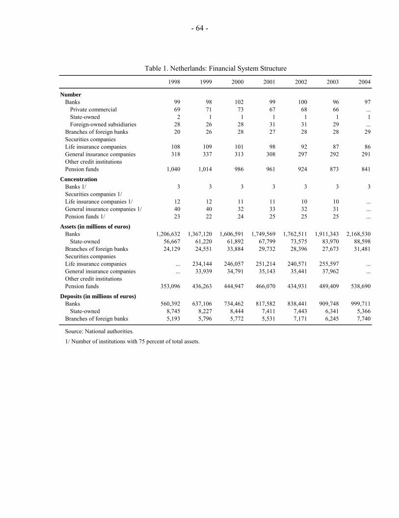
- 64 -

1998 1999 2000 2001 2002 2003 2004

NumberBanks 99 98 102 99 100 96 97

Private commercial 69 71 73 67 68 66 ...State-owned 2 1 1 1 1 1 1Foreign-owned subsidiaries 28 26 28 31 31 29 ...

Branches of foreign banks 20 26 28 27 28 28 29Securities companiesLife insurance companies 108 109 101 98 92 87 86General insurance companies 318 337 313 308 297 292 291Other credit institutionsPension funds 1,040 1,014 986 961 924 873 841

ConcentrationBanks 1/ 3 3 3 3 3 3 3Securities companies 1/Life insurance companies 1/ 12 12 11 11 10 10 ...General insurance companies 1/ 40 40 32 33 32 31 ...Pension funds 1/ 23 22 24 25 25 25 ...

Assets (in millions of euros)Banks 1,206,632 1,367,120 1,606,591 1,749,569 1,762,511 1,911,343 2,168,530

State-owned 56,667 61,220 61,892 67,799 73,575 83,970 88,598Branches of foreign banks 24,129 24,551 33,884 29,732 28,396 27,673 31,481Securities companiesLife insurance companies ... 234,144 246,057 251,214 240,571 255,597 ...General insurance companies ... 33,939 34,791 35,143 35,441 37,962 ...Other credit institutionsPension funds 353,096 436,263 444,947 466,070 434,931 489,409 538,690

Deposits (in millions of euros)Banks 560,392 637,106 734,462 817,582 838,441 909,748 999,711

State-owned 8,745 8,227 8,444 7,411 7,443 6,341 5,366Branches of foreign banks 5,193 5,796 5,772 5,531 7,171 6,245 7,740

Source: National authorities.

1/ Number of institutions with 75 percent of total assets.

Table 1. Netherlands: Financial System Structure

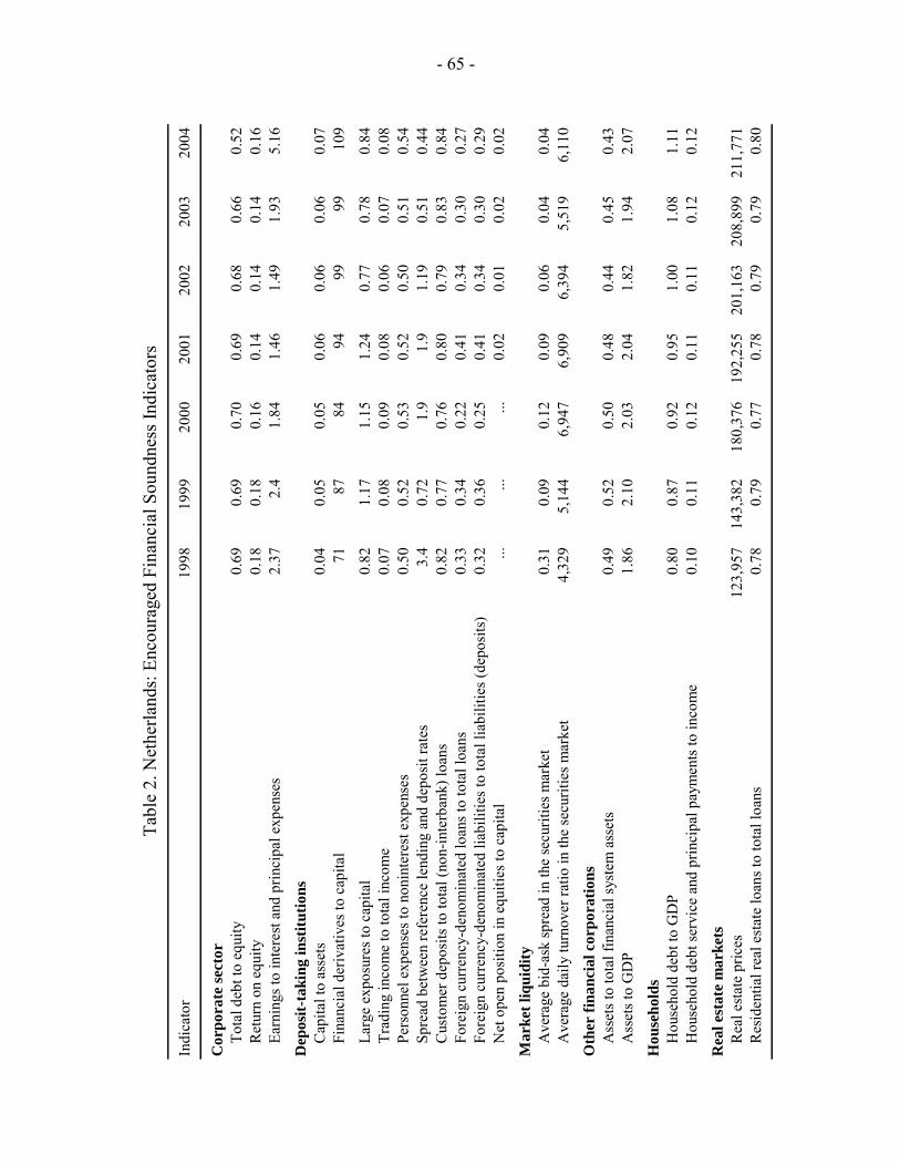
- 65 -

Indi

cato

r19

9819

9920

0020

0120

0220

0320

04

Cor

pora

te se

ctor

Tota

l deb

t to

equi

ty0.

690.

690.

700.

690.

680.

660.

52R

etur

n on

equ

ity0.

180.

180.

160.

140.

140.

140.

16Ea

rnin

gs to

inte

rest

and

prin

cipa

l exp

ense

s2.

372.

41.

841.

461.

491.

935.

16

Dep

osit-

taki

ng in

stitu

tions

Cap

ital t

o as

sets

0.04

0.05

0.05

0.06

0.06

0.06

0.07

Fina

ncia

l der

ivat

ives

to c

apita

l71

8784

9499

9910

9

Larg

e ex

posu

res t

o ca

pita

l0.

821.

171.

151.

240.

770.

780.

84Tr

adin

g in

com

e to

tota

l inc

ome

0.07

0.08

0.09

0.08

0.06

0.07

0.08

Pers

onne

l exp

ense

s to

noni

nter

est e

xpen

ses

0.50

0.52

0.53

0.52

0.50

0.51

0.54

Spre

ad b

etw

een

refe

renc

e le

ndin

g an

d de

posi

t rat

es3.

40.

721.

91.

91.

190.

510.

44C

usto

mer

dep

osits

to to

tal (

non-

inte

rban

k) lo

ans

0.82

0.77

0.76

0.80

0.79

0.83

0.84

Fore

ign

curr

ency

-den

omin

ated

loan

s to

tota

l loa

ns0.

330.

340.

220.

410.

340.

300.

27Fo

reig

n cu

rren

cy-d

enom

inat

ed li

abili

ties t

o to

tal l

iabi

litie

s (de

posi

ts)

0.32

0.36

0.25

0.41

0.34

0.30

0.29

Net

ope

n po

sitio

n in

equ

ities

to c

apita

l...

......

0.02

0.01

0.02

0.02

Mar

ket l

iqui

dity

Ave

rage

bid

-ask

spre

ad in

the

secu

ritie

s mar

ket

0.31

0.09

0.12

0.09

0.06

0.04

0.04

Ave

rage

dai

ly tu

rnov

er ra

tio in

the

secu

ritie

s mar

ket

4,32

95,

144

6,94

76,

909

6,39

45,

519

6,11

0

Oth

er fi

nanc

ial c

orpo

ratio

nsA

sset

s to

tota

l fin

anci

al sy

stem

ass

ets

0.49

0.52

0.50

0.48

0.44

0.45

0.43

Ass

ets t

o G

DP

1.86

2.10

2.03

2.04

1.82

1.94

2.07

Hou

seho

lds

Hou

seho

ld d

ebt t

o G

DP

0.80

0.87

0.92

0.95

1.00

1.08

1.11

Hou

seho

ld d

ebt s

ervi

ce a

nd p

rinci

pal p

aym

ents

to in

com

e0.

100.

110.

120.

110.

110.

120.

12

Rea

l est

ate

mar

kets

Rea

l est

ate

pric

es12

3,95

714

3,38

218

0,37

619

2,25

520

1,16

320

8,89

921

1,77

1R

esid

entia

l rea

l est

ate

loan

s to

tota

l loa

ns0.

780.

790.

770.

780.

790.

790.

80

Tabl

e 2.

Net

herla

nds:

Enc

oura

ged

Fina

ncia

l Sou

ndne

ss In

dica

tors

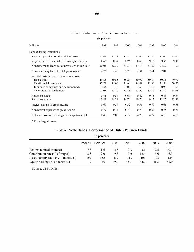
- 66 -

Indicator 1998 1999 2000 2001 2002 2003 2004

Deposit-taking institutionsRegulatory capital to risk-weighted assets 11.41 11.18 11.25 11.44 11.86 12.05 12.07Regulatory Tier I capital to risk-weighted assets 8.65 8.57 8.76 8.63 9.13 9.55 9.91Nonperforming loans net of provisions to capital * 30.05 32.32 31.34 31.13 31.22 24.32 ...

Nonperforming loans to total gross loans * 2.72 2.48 2.25 2.31 2.41 2.01 ...

Sectoral distribution of loans to total loansHouseholds 49.85 50.85 50.20 50.92 50.80 50.31 49.92Nonfinancial companies 37.79 35.96 35.94 34.48 32.60 31.56 29.72Insurance companies and pension funds 1.33 1.10 1.08 1.63 1.43 0.98 1.67Other financial institutions 11.03 12.10 12.78 12.97 15.17 17.15 18.69

Return on assets 0.44 0.57 0.60 0.42 0.35 0.46 0.54Return on equity 10.89 14.29 14.74 10.76 9.17 12.27 13.81

Interest margin to gross income 0.60 0.57 0.52 0.56 0.60 0.61 0.58

Noninterest expenses to gross income 0.79 0.74 0.73 0.79 0.82 0.75 0.71

Net open position in foreign exchange to capital 8.45 9.08 6.17 4.78 4.27 6.13 4.10

* Three largest banks.

Table 3. Netherlands: Financial Sector Indicators(In percent)

1990-94 1995-99 2000 2001 2002 2003 2004

Returns (annual average) 7.3 11.6 2.5 -2.8 -0.1 12.5 10.1Contribution rate (% of wages) 8.5 9.0 9.5 10.0 12.4 15.0 16.3Asset-liability ratio (% of liabilities) 107 135 132 118 101 108 124Equity holding (% of portfolio) 19 46 49.0 48.3 42.3 46.3 46.9

Source: CPB, DNB.

Table 4. Netherlands: Performance of Dutch Pension Funds(In percent)