international monetary policy - london school of economicspersonal.lse.ac.uk/piffer/lecture slides...

International Monetary Policy7 IS-LM Model 1

Michele Piffer

London School of Economics

1Course prepared for the Shanghai Normal University, College of Finance, April 2011Michele Piffer (London School of Economics) International Monetary Policy 1 / 56

Lecture topic and references

I In this lecture we construct a simple macroeconomic model that helpsunderstand what happens after monetary policy contractions andexpansions

I Mishkin, Chapter 20

Michele Piffer (London School of Economics) International Monetary Policy 2 / 56

Review from previous lecture

Open Market Operations Discount Conditions Reserve Requirements Communication of Fed Funds Target

Reserve Aggregates (Monetary Base)

Short-term Interest Rates (Fed Funds Rate)

Monetary Aggregates (M1 M2)

Long-term Interest Rates

Inflation Expectations

Price Stability

High Employment Financial Stability Economic Growth

Tools Policy Instruments Intermediate Targets Goalss


We need some theory

I So far we have learnt how Central Banks behave. What we need nowis some understanding of the impact of monetary policy on the entireeconomy

I The model we will study in this lecture helps predict the impact ofboth monetary and fiscal policies, at least in the short run when pricesare fixed

I We will start by constructing the model, which is a simplereduced-form model of 2 equations in 2 unknowns. Afterwards, wewill use it for some policy analysis


The IS-LM model in a Nutshell

I The IS-LM model is the theoretical synthesis of the Keynesian way ofthinking about macroeconomics

I It reflects what Keynes had in mind when he wrote The GeneralTheory of Employment, Interest, and Money, published in year 1936.But the model was formalized by Sir John Hicks in year 1937


The IS-LM model in a Nutshell

I The key intuition is that aggregate output/production/income (theyare the same) reflect the equilibrium between aggregate demand (bymarket players) and aggregate supply (by firms)

I To the extend that policymakers can influence aggregate demand,aggregate supply will follow and the economy will move towards adesired equilibrium (at least in the short run)


Determinants of Aggregate Demand

I Let’s start with a simplified version of the model, where the onlymarket considered is the goods market (we will introduce the moneymarket shortly)

I By aggregate supply Y as we mean the total production of goods inan economy. It clearly comes from firms

I Aggregate demand comes instead from a variety of economic players.In general:

Y ad = C + I + G + CA

withI C = ConsumptionI I = InvestmentI G = Government SpendingI NX = Net Exports



I The equilibrium in the goods market will be given by an effective levelof production Y where

Y as = Y ad = Y

I The point of the model is to determine the level of output Y ∗ so thatthe corresponding aggregate demand Y ad is exactly equal to Y ∗

I In order to do this we need to come up with some theory of thecomponents of aggregate demands, and then derive the equilibrium



I Start from the simplified case where G = NX = 0

I Assume C = a + mpc · Y d , whereI a = autonomous consumer expenditureI mpc = marginal propensity to consume (between 0 and 1)I Y d = disposable income = Y − T (here T=0)

I Assume for the moment that investments by firms are determinedexogenously (i.e. not inside the model), i.e. I = I0 (we will abandonthis restrictive assumption shortly)

I This means that Y ad = a + mpc · Y + I0



I The key intuition is that aggregate demand depends positively onoutput, so there will be only one level of output whose correspondingaggregate demand is exactly equal to that output

I In order to characterize that level of output one can proceed in twoways:

I Approach a): Solve for the reduced form of Y after imposingY = Y ad

Y = a + mpc · Y + I0

I Solving for Y one gets

Y ∗ =1

1 − mpc· (a + I0) (1)

I Note, 11−mpc > 1



I Before interpreting the above result, let’s see the other approach:

I Approach b): Compare graphically Y ad and Y

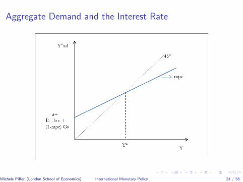
I Note, on the space (Y ad , Y ) the function Y ad is a line with intercepta + I0 and slope mpc

I What happens if I0 increases by 1? Graphically, the Y ad shifts up;analytically, equation (2) shows that

∆Y ∗ =1

1 − mpc∆I0



I How is it possible that an increase in the exogenous investment by 1increase equilibrium output by more than 1?

I The intuition is the following: as firms demand for one extra good,some other firm will produce that extra good

I This means that some consumer will earn a higher disposable income,since the profits (or simply the wage) from producing that extra goodmust go somewhere. As consumption increases, aggregate demandincreases again, triggering the same mechanism

I This mechanism is called multiplication process. For this reason wecall 1

1−mpc the expenditure multiplier


Introducing Government Expenditure

I Let’s abandon now the restrictive assumption that there is nogovernment expenditure

I Assume G = G0. Under balanced budget we have G = T , henceY d < Y


Introducing Government Expenditure

I In this new setting aggregate demand will be given by

Y = a + mpc · (Y − T ) + I0 + G0

I Solving for Y one gets (substituting G = T )

Y ∗ =1

1 − mpc· (a + I0 + (1 − mpc) · G0) (2)

I Note that the multiplier on the government expenditure is 1. Let’ssee this graphically


Aggregate Demand with Government Spending


Aggregate Demand with Government Spending

I When government expenditure increases by 1 the government isincreasing taxes by 1. How can it be that equilibrium output stillincreases, given that what the government gives is equal to what ittakes away?

I The point is that an extra unit of government expenditure increaseaggregate demand by 1, while an increase in taxation by 1 decreasesaggregate demand mpc < 1, so that, on impact, aggregate demandincreases and starts the multiplication mechanism described before

I Under constant interest rate (as in this case) the fiscal multiplier is

∆Y ∗

∆G= 1


Exercise 1 on Aggregate Demand

I Suppose that a = 2, mpc = 0.5, I0 = 10 and there is no government.Show the equilibrium condition graphically and compute theequilibrium output. What is the value of aggregate demand inequilibrium?

I Suppose that the exogenous investments increase up to 15. What doyou expect to happen to equilibrium output? Do the above steps andcheck your prediction


Exercise 2 on Aggregate Demand

I Suppose that a = 2, mpc = 0.5, I0 = 10. The government runs abalance budget equal to 10. Show the equilibrium conditiongraphically and compute the equilibrium output. What is the value ofaggregate demand in equilibrium?

I Suppose that government expenditure increases by 2. What do youexpect to happen to equilibrium output? Do the above steps andcheck your prediction


Aggregate Demand and the Interest Rate

I So far we have assumed that investments are exogenous, that is,depend on so called animal spirits

I If we think about it, it makes sense to assume that investments arenegatively related to the interest rate



I Remember, by investments we mean, for instance, firms deciding tobuy a new machinery for their production

I In doing so firms need to borrow money from savers, and will issuebonds with a contractual interest rate

I The higher is the interest rate and the higher the cost of money,hence the lower the incentive to invest (net present value of futurecash flows decreases)



I Assume that investments have an exogenous component I0 and anendogenous component that depends negatively on the interest rate,according to a factor b

I = I0 − b · r

I Under this new environment aggregate demand is given by

Y = a + mpc · (Y − T ) + I0 − b · r + G0

I Following the same steps we get

Y ∗ =1

1 − mpc· (a + I0 − b · r + (1 − mpc) · G0) (3)



I Note, equilibrium output Y ∗ is negatively related to the interest rate,as clearly displayed by (3). This is because a higher interest ratewould reduce investments, decrease aggregate demand and henceequilibrium output

I Equation (3) provides one of the two key equations of the model

I So far the only endogenous variable was Y , which was representingthe equilibrium variable for the goods market. But a monetary modelof course considers the interest rate as well as an endogenous variable

I We will derive the second equation after we introduce the moneymarket


IS Curve

I Let’s rewrite (3) in a more convenient form. We will refer to this asthe IS curve

Y ∗ =1

1 − mpc· (A − b · r) (IS)

with A = a + I0 + (1 − mpc) · G0, defined as the autonomousaggregate demand

I The IS curve is defined as the combination of (r , Y ) where the goodsmarket is in equilibrium. Any disequilibrium will be eliminated byvariations in output


IS Curve

I The IS curve is negatively sloped on the the space (r , Y ): higherinterest rate reduces investments, aggregate demand and henceequilibrium output

I Above the curve we have excess supply of goods; equilibrium outputwill decrease since firms realize that they are producing too much

I Below the curve we have excess demand of goods; equilibrium outputwill increase since firms realize that they are producing too little


IS Curve


Exercise 1 on IS curve

I Consider the following figure and complete the next slide:


Exercise 1 on IS curve

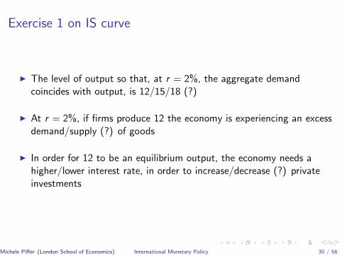
I The level of output so that, at r = 2%, the aggregate demandcoincides with output, is 12/15/18 (?)

I At r = 2%, if firms produce 12 the economy is experiencing an excessdemand/supply (?) of goods

I In order for 12 to be an equilibrium output, the economy needs ahigher/lower interest rate, in order to increase/decrease (?) privateinvestments


Money Market

I Money supply is provided by the Central Bank. We have seen that itscontrol is not perfect, as there are important factors affecting moneysupply that depend on market participants

I In this model we assume that money supply is perfectly controlled bythe CB. Call Ms the nominal amount of money

I It follows that the real amount of money supply will be given by

Ms

P


Money Market

I How do we pin down real money demand?

I Transaction motive: people demand money for doing transactions, sothe higher output and the higher money demand

I At the same time people might decide to allocate their wealth intoassets, instead of money


Money Market

I There is a clear trade off: money is by definition liquid, so can beused for transaction. But it yields no interest rate

I Speculative motive: The higher the interest rate and the higher theincentive to shift from money to assets. The higher the interest rateand the lower the real money demand


Money Market

I Remember, we saw that on the goods market an increase in interestrate reduces investments. This was because firms will have to paysuch interest rate

I The point is that savers are on the other side: they will earn theinterest rate as soon as they decide to allocate part of their wealth toassets

I Do not confuse the idea of investment with the allocation of savingsinto financial instruments. Investment means physical investments


Money Market

I Having established a money demand and a money supply, we onlyneed to impose equilibrium and pin down the second equation of themodel

I Write money demand as

Md = L(Y+

, r)

where the signs under Y and r indicate partial derivatives


Money Market

I Imposing equilibrium on the money market gives

Ms

P= L(Y

+, r) (LM)

I The above equation capture the LM curve: combinations of incomeand interest rate that allow for the equilibrium in the money market


Money Market

I One can study the LM curve either on the (r , M) space or on the(r , Y ) space

I On the (r , M) space the Real Money Supply is vertical, while theMoney Demand is negatively sloped


Money Market


Money Market

I A situation of excess money supply will lead to a reduction of the costof money: firms will find it easier to issue bonds as the market is fullof liquidity, so will pay a lower interest rate

I Similarly, a situation of excess money demand will lead to an increasein the cost if money: firms issuing bonds will struggle to raise fundsand will have to increase the interest rate paid


Disequilibrium in the Money Market


Money Market

I Note: as income increases, money demand shifts to the right. Thiscreates an excess of money demand and a consequent increase in theinterest rate. This means that the LM curve implies a positiverelation between Y and r

I Note: the movement in the interest rate allows the market to moveback to equilibrium. In case of excess of money demand (supply)interest rate will increase (decrease), hence reducing (increasing)money demand and leading the money market to equilibrium


Money Market: Y and r are positively related


Money Market

I How does the LM curve look like on the (r , Y ) space?

I It is positively sloped: an increase in income increase money demand.Given that money supply is exogenous, we need an increase of theinterest rate to decrease money demand and guarantee theequilibrium on the money market

I The adjusting variable on the money market is the interest rate (onthe goods market it was output)


LM curve


Exercise 1 on LM curve

I Consider the following figure and complete the next slide


Exercise 1 on LM curve

Assume nominal Money Supply equals 20, level of prices equals 2. Then

I At point A Money Demand (= / > / <)10, interest rate will increase/decrease/stay constant (?)

I At point B Money Demand (= / > / <)10, interest rate will increase/decrease/stay constant (?)

I At point C Money Demand (= / > / <)10, interest rate will increase/decrease/stay constant (?)

I At point D Money Demand (= / > / <)10, interest rate will increase/decrease/stay constant (?)


The IS - LM Model

I Let’s sum up: the IS-LM model studies the equilibrium in twomarkets, the goods market and the money market

I The endogenous variables are income Y and the interest rate r

I The equilibrium conditions are captured by two curves, the IS curveand the LM curve

I Output / interest rate adjustment allow the system to reach anequilibrium where both markets clear


IS - LM Model


What happens in point A ?


Adjustment Mechanisms

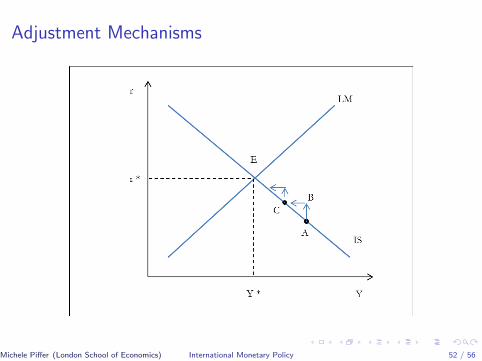
I Since goods market is in equilibrium, output will not change. But theexcess demand of money will lead to an increase in the interest rate,which starts closing the gap of excess money demand (point B)

I As interest rate increases the goods market gets out of equilibrium:incentive to invest have decreased, so aggregate demand has fallen,but aggregate output has not. This will lead firms to decreaseproduction (point C)

I The mechanism continues until the economy reaches point E


What happens in point A ?



I Since money market is in equilibrium, interest will not change. Butthe excess supply of goods will lead firms to reduce production, whichstarts closing the gap on the goods market (point B)

I As output decreases the money market gets out of equilibrium:demand for money decreases due to reduced transaction motive,pushing interest rate to fall (point C). Note that the fall in r increasesinvestment and closes the gap on the goods market

I The mechanism continues until the economy reaches point E


Plan for the Future

I Economic policies will shift the IS and / or LM curve

I Use the model to understand the impact of different economicpolicies on the equilibrium of the economy

I After covering International Economics we will reframe the model toallow for NX different than zero


international monetary policy - london school of economicspersonal.lse.ac.uk/piffer/lecture slides...

Documents