international review on modelling and simulations
TRANSCRIPT

International Review on
Modelling and Simulations (IREMOS)
Contents
Sensorless Fuzzy MPPT Technique of Solar PV and DFIG Based Wind Hybrid System
by Marouane El Azzaoui, Hassane Mahmoudi, Karima Boudaraia
152
Analysis of Flashover Induced by Transient Current During Multiple Lightning Strokes on a Train
by Kelvin M. Minja, Pius V. Chombo, Narupon Promvichai, Boonruang Marungsri
160
Performance Analysis of a Wind Turbine Based on a Self-Excited Induction Generator (SEIG)
by Abdallah Belabbes, Mohamed Bouhamida, Allal El Moubarek Bouzid, Mustapha Benghanem, Mohamed Della-Krachai, Mamadou Lamine Doumbia
169
Seawater Desalination Pilot Plant: Optimal Design and Sizing of Solar Driven-Four Effect Evaporators Combined with Heat Integration Analysis
by M. Ghazi, E. Essadiqi, M. Mada, M. Faqir, A. Benabdellah
177
Forest Fire Danger Assessment Using SPMD-Model of Computation for Massive Parallel System
by Nikolay V. Baranovskiy
193
Rule-Based and Genetic Algorithm for Automatic Gamelan Music Composition
by Khafiizh Hastuti, Azhari, Aina Musdholifah, Rahayu Supanggah
202

International Review on Modelling and Simulations (I.RE.MO.S.), Vol. 10, N. 3
ISSN 1974-9821 June 2017
Copyright © 2017 Praise Worthy Prize S.r.l. - All rights reserved https://doi.org/10.15866/iremos.v10i3.11361
152 152 152
Sensorless Fuzzy MPPT Technique of Solar PV and DFIG Based Wind Hybrid System
Marouane El Azzaoui, Hassane Mahmoudi, Karima Boudaraia Abstract – This paper presents a method for estimating the power of a PV combined with a wind system based on a Doubly Fed Induction Generator (DFIG). This estimated power is used for calculating the maximum power point tracking algorithm. A turbine drives the DFIG, its stator is attached directly to the grid, while its rotor is connected to the grid through a back-to-back converter. The PV system is used with a buck-boost converter, which is linked to the DC bus of the back-to-back converter. This structure eliminates the inverter with its associated devices. In this work, the MPPT algorithm is based on fuzzy logic whose inputs are: the previous duty cycle and the estimated power based on the calculation made by the DFIG. This allows removing the voltage and current sensors. The simulation results present the performance of the proposed method subjected to irradiation and wind speed variations at different operating modes. Copyright © 2017 Praise Worthy Prize S.r.l. - All rights reserved. Keywords: Sensorless MPPT, Photovoltaic, Doubly Fed Induction Generator, Fuzzy MPPT,
Hybrid System
Nomenclature
pvI Output current of the solar cell
pvV Output voltage of the solar cell
phI Photocurrent produced by PV cell
sI Reverse saturation current of diode q Electric charge of electron k Boltzmann constant n Ideality factor
seR , shR Series and shunt resistances
sdV , sqV Direct and quadratic stator voltages of DFIG
sdI , sqI Direct and quadratic stator currents of DFIG
sd , sq Direct and quadratic stator flux of DFIG
rdV , rqV Direct and quadratic rotor voltages of DFIG
rdI , rqI Direct and quadratic rotor currents of DFIG
rd , rq Direct and quadratic rotor flux of DFIG
sR , rR Stator and rotor resistor
s , r Stator and rotor frequencies
sL , rL , mL Stator, rotor and mutual inductances p Pole pair number
m Mechanical speed of the DFIG
sP , rP Stator and rotor active power
sQ , rQ Stator and rotor reactive power
Leakage coefficient g Slip Air density
pC Power coefficient Pitch angle R Radius of the turbine
wv Wind speed Tip speed ratio
t Angular speed of the turbine
mT Torque of the turbine
LT Load torque J Moment of inertia of the turbine f Viscosity coefficient of the turbine
I. Introduction Renewable energy has seen an increase in recent years
to reduce fossil energy sources such as oil, gas, and coal polluting the environment. These renewable energy, wind and solar energies are considered the most potential. The development of power electronics makes photovoltaic energy and wind system more attractive and practical. Moreover, DFIG becomes popular due to its advantages in variable speed wind turbine [1], [2].
The combination of DFIG and PV has several advantages compared with separate DFIG and PV such as the reduction of the system cost. The chosen structure of the hybrid system is built on a back-to-back converter connected to the rotor of the DFIG while the PV system provides power through a buck-boost converter that is

M. El Azzaoui, H. Mahmoudi, K. Boudaraia
Copyright © 2017 Praise Worthy Prize S.r.l. - All rights reserved International Review on Modelling and Simulations, Vol. 10, N. 3
153
linked to the DC bus of the back-to-back converter. There is in literature many hybrid system based on
DFIG and PV. For example, Rajesh et al. give an architecture and control of the hybrid system [3]. Chin Kim Gan et al. present a paper that assesses the potential of implementing the Hybrid Diesel/PV/Wind/Battery in Eluvaitivu Island using HOMER simulation [4]. Mukwanga W. Siti use a load following diesel dispatch strategy and analyse the fuel costs and energy flows [5]. Benameur Afif et al. present a wind/PV hybrid system in rural areas [6]. This research presents a sensorless Fuzzy MPPT technique to estimate the PV power for the hybrid system, which eliminates more the voltage sensor compared to old research, which eliminate just the current sensors like the work of Nguyen and Fujita that introduced a sensorless method using P&O MPPT algorithm, which remove only the current sensor of PV [7].
This research is arranged as follow: a brief structure of the system is presented in second section, and the modelling of the DFIG and PV is illustrated in the third section, while the fourth section summarizes the control strategy of the DFIG, establishing the Fuzzy MPPT algorithm, and presenting a sensorless technique to estimate PV power. Finally, simulation results show the response of the proposed method under changes of irradiation and wind speed.
II. Presentation of the Studied System The system studied in this work is shown in Fig. 1.
The turbine is connected to DFIG through a gearbox, which allows adapting the low speed rotation of the turbine to high speed of the DFIG. The stator of the DFIG is connected directly to the grid, while its rotor is connected to the grid through a back-to-back converter and RL filter that help mitigate harmonic generated by this converter. The PV generates a power which is the input to DC-DC converter, while its output is related to DC-link of the Back-to-Back converter, then the RSC and GSC convert the DC energy to AC energy which supplies the rotor or the grid depending on the operating mode (hypo-synchronous or hyper-synchronous) [14], [15]. The DC-DC converter used is a buck-boost converter, which has good stability and fast response. The advantage of this structure is that the inverter with it associated components most used after the buck-boost converter is eliminated which reduces the system cost. Furthermore, a senseless technique for the hybrid system is suggested. This technique decrease the numbers of sensors used to extract the maximum power of the PV, so that reduces more the system cost.
III. Modelling of PV and DFIG To control the hybrid system, it is necessary to model
the PV and DFIG. Modelling means bring out the mathematical equations governing the physical behaviour of the system.
Fig. 1. Structure of the hybrid system
III.1. Modelling of PV
The equivalent circuit of a photovoltaic cell consists of a photo current, a diode, a shunt resistor that expresses the leakage current, and a series resistor defines the internal resistor which limits the current (Fig. 2).
Fig. 2. Equivalent circuit of a PV cell
Equation describing the voltage-current characteristic is given by [8]:
1pv se pv
pv ph s
pv se pv
sh
q V R II I I exp
nkT
V R IR
(1)
Fig. 3 presents the P-V and I-V characteristics of the
PV array. We notice that the characteristic of the power in function as voltage presents a maximum power point (MPP). In order to extract the maximum power, this point must be tracked whatever the weather conditions.
III.2. Modelling of DFIG
The DFIG is modelled in d-q frame reference by the following equations [9]:

M. El Azzaoui, H. Mahmoudi, K. Boudaraia
Copyright © 2017 Praise Worthy Prize S.r.l. - All rights reserved International Review on Modelling and Simulations, Vol. 10, N. 3
154
Fig. 3. Power-Voltage curves under irradiation and temperature change
Voltage equations:
sdsd s sd s sq
dV R I
dt
(2)
sqsq s sq s sd
dV R I
dt
(3)
rdrd r rd r rq
dV R I
dt
(4)
rqrq r rq r rd
dV R I
dt
(5)
Flux equations: sd s sd m rdL I L I (6) sq s sq m rqL I L I (7) rd r rd m sdL I L I (8) rq r rq m sqL I L I (9) Frequencies equation: r s mp (10) Powers equations: s sd sd sq sqP V I V I (11) s sq sd sd sqQ V I V I (12) r rd rd rq rqP V I V I (13) s rq rd rd rqQ V I V I (14)
In this step, the stator field orientation is applied by aligning the stator flux with d axis to simplify the control of the DFIG [10]. Moreover, considering that the grid fed the generator by a stable voltage, and neglecting the stator resistor [11], we obtain:
0sd s sq; (15) 0sd sq s s sV ; V V (16)
These assumptions led to deducing the expressions of the rotor voltages:
rdrd r rd r r s rq
dIV R I L g L I
dt (17)
rq s mrq r rq r r s rd
s
dI V LV R I L g L I g
dt L (18)
The powers can be simplified as:
s ms rq
s
V LP I
L (19)
2
s m ss rd
s s s
V L VQ I
L L (20)
From equation (19) and equation (20), it is obvious
that we can control independently the stator active and reactive powers by controlling the rotor currents. Hence, the reference currents are calculated from these equations.
IV. Sensorless Control of the Hybrid System
The control of the hybrid system is depicted in this section. First, classical controls of the DFIG and PV MPPT are highlighted. The sensorless method of MPPT power is suggested secondly.
IV.1. Maximum Power of Wind Turbine
Wind turbine produces the following power [12]:
2 30 5m p wP . C , R v (21) where ρ is the air density, Cp is the power coefficient, β is the blades orientation, R is the radius of the turbine, vw is the wind speed, and λ is the tip speed ratio, which is given by:
t
w
Rv
(22)
where Ωt is the angular speed of the turbine, its dynamic is given by:
tm L t
dJ T T f
dt
(23)

M. El Azzaoui, H. Mahmoudi, K. Boudaraia
Copyright © 2017 Praise Worthy Prize S.r.l. - All rights reserved International Review on Modelling and Simulations, Vol. 10, N. 3
155
where J is the moment of inertia, f is the viscosity coefficient, Tm is the torque generated by the turbine, and TL is the load torque in this case the electromagnetic torque of the DFIG. The maximum power that can be developed by the turbine is written as:
5
33
0 5 pmaxmax topt
opt
. R CP
(24)
with:
opt wtopt
vR
(25)
IV.2. RSC Control
Through the rotor side converter (RSC), we can control the active and reactive powers of the generator independently, from equation (19) and equation (20), those powers are controlled by controlling the rotor currents using PI correctors. Results voltages are converted in the abc reference frame using Park inverse. Thereafter, by comparing these voltages with a carrier signal, the switching signals are generated to control the IGBTs of the converter as presented in Fig. 4 [16]-[18].
Fig. 4. RSC control strategy
IV.3. GSC Control
Control strategy of the grid side converter (GSC) allows controlling the reactive power passing through the filter and therefore the power factor, and regulating the DC bus voltage to a constant value enough to have three-phase voltages to the other side of RSC and GSC. The reactive power is controlled by regulating the d-axis current using a PI controller. The control of the DC bus voltage is done through two regulation loops, an outer loop that regulates the DC voltage and an inner loop that control the q-axis current by using also the PI controller to track the reference signal. Results voltages are
transformed to abc frame using Park inverse which its angle is obtained using a PLL, and compared with the carrier signal to get the pulse width modulation necessary to control the IGBTs of the converter. Fig. 5 describes the control of the GSC.
Fig. 5. GSC control strategy
IV.4. Maximum Power of PV
MPPT is a technique that maximizes the power of the PV by adjusting the voltage to follow the top of the P-V curve. The voltage is adjusted by tightening the duty cycle of the buck-boost converter that adapts the power of the PV system to the load. There are several MPPTs algorithm in the literature. The most familiar is the P&O. In this work, the fuzzy MPPT is adopted because it robust than the P&O technique, and the other reason for choosing this method is that the input is the change of power and the previous duty cycle, therefore in the sensorless step, the voltage sensor is removed again compared to the work done here [7]. The principal of the fuzzy controller based maximum power point tracking is presented in Fig. 6. Voltage and current are measured and then used to calculate the power. The fuzzy system handles the two inputs change of power ΔPk multiplied by the scaling factor kp and the previous value of the duty cycle ΔDk-1 to provide the duty cycle Dk that converted to PWM signal to control the switch of the buck-boost converter. kd is the scale factor in the output, and 1Z is a unity delay [13].
Fig. 6. Scheme of MPPT using Fuzzy logic

M. El Azzaoui, H. Mahmoudi, K. Boudaraia
Copyright © 2017 Praise Worthy Prize S.r.l. - All rights reserved International Review on Modelling and Simulations, Vol. 10, N. 3
156
Fig. 7 and Fig. 8 show the subsets of the input and output to the fuzzy system. Input ∆Pk has five fuzzy subsets Positive Big (PB), Positive Small (PS), Zero (ZE), Negative Small(NS), and Negative Big (NB). Input ∆Dk−1 and output ∆Dk have eleven fuzzy subsets PB, Positive Medium (PM), Positive Medium Medium (PMM), PS, Positive Small Small (PSS), ZE, Negative Small Small (NSS), NS, Negative Medium Medium (NMM), Negative Medium (NM), and NB. The inputs and output are normalized. The membership functions are made by triangular and trapezoidal shapes and are denser in the centre to have good accuracy while the variation of power close to zero.
Fig. 7. Membership functions power input
Fig. 8. Previous duty cycle input and duty cycle output membership functions
The fuzzy rules are defined by analysis of the PV
behaviour. All conditions are taken into account to achieve good performance in term of tracking the maximum point. The Fuzzy rules are summarized in Table I.
TABLE I
FUZZY SYSTEM RULES
∆Dk ∆Dk−1
NB NM NMM NS NSS ZE PSS PS PMM PM PB
∆Pk
NB PM PMM PS PSS PSS NB NSS NSS NS NMM NM NS PM PMM PS PSS PSS NS NSS NSS NS NMM NM ZE NB NM NMM NS NSS ZE PSS PS PMM PM PB PS NM NMM NS NSS NSS PS PSS PSS PS PMM PM PB NM NMM NS NSS NSS PB PSS PSS PS PMM PM
Fig. 9 shows the graphical representation of the fuzzy
surface.
IV.5. Sensorless of PV Power
Maximizing power method of the PV is based on the measurement of power by measuring voltage and current as illustrated in Fig. 6.
Fig. 9. Surface generated by fuzzy system In this section, a sensorless technique is shown to
estimate the power used in the input of the fuzzy system to track the maximum power point of the PV and therefore eliminate the voltage and current sensors. This sensorless method is based on measurements made by the DFIG such as the output of the buck-boost converter is linked to the DC bus of the DFIG.
Fig. 10 shows the flows of powers exchanged between the PV and DFIG in the two hypo-synchronous and hyper-synchronous modes. In hypo-synchronous 1 mode, the direction of transfer of the energy comes from the grid and PV to the rotor of the machine, while a part of energy produced by the PV if and only so great is injected to the grid in hypo-synchronous 2 mode.
Fig. 10. Flow of powers exchanged between the converters
Finally, the power produced by the rotor of the DFIG and the PV are injected directly to the grid. The flow of all power in different operating mode is expressed by: In hypo-synchronous mode 1:
rsc gsc pvP P P (26) In hypo-synchronous mode 2:
pv rsc gscP P P (27)

M. El Azzaoui, H. Mahmoudi, K. Boudaraia
Copyright © 2017 Praise Worthy Prize S.r.l. - All rights reserved International Review on Modelling and Simulations, Vol. 10, N. 3
157
In hyper-synchronous mode : gsc rsc pvP P P (28) where Prsc is the RSC power, and Pgsc is GSC power, their expressions are given by: rsc ra a rb b rc s dcP i S i S i S V (29) gsc fa a fb b fc s dcP i S i S i S V (30) here subscripts r, f, a, b, and c are rotor side, filter side, phase a, phase b, and phase c respectively. Sa,b,c is the switching states of the RSC and GSC.
Table II summarizes the different systems and sensors used. Separate PV-DFIG needs all the sensors, the hybrid system without using the sensorless technique eliminate the PV inverter, when the sensorless technique is used with P&O MPPT which presented here [7], the current sensor is removed again. Moreover, the sensorless with fuzzy logic system presented in this paper eliminate the voltage sensors.
TABLE II
COMPARATIVE SENSORLESS TECHNIQUES Sensor
System
DFIG sensors
Vpv sensor Ipv sensor PV inverter
Separate PV-DFIG Yes Yes Yes Yes
Hybrid without Sensorless Yes Yes Yes No
Sensorless with P&O MPPT Yes Yes No No
Sensorless with fuzzy MPPT Yes No No No
V. Simulation Results The entire system is simulated using Matlab/Simulink
software. The proposed MPPT and estimated power are analysed under change of irradiation. The flow of powers is validated in the different operating mode. The irradiation is increased from 0.6 pu to 1 pu at t=0.5s and decreased from 1 pu to 0.8 pu at t=0.7s as shown in Fig. 11.
Fig. 11. Change of irradiation
Under this change of irradiation, the power is retained in the optimal value as depicted in Fig. 12, and the Fig. 13 shows that DC bus voltage is kept to its constant
reference value. The estimated power is almost equal to the power measured unless a simple error due to the buck-boost converter yield (Fig. 14).
Fig. 12. MPPT under change of irradiation
Fig. 13. Evolution of the DC bus Voltage
Fig. 14. Response of measured and estimated powers
Now the system is subject to the variation of irradiation and wind speed to analyse the flow of powers exchanged between all converters. In hypo-synchronous 1 mode, Irradiation was increased from 1 pu to 0.8 pu at t=0.6s and wind speed is decreased from 0.9 pu to 0.8 pu at t=0.8s.
Fig. 15 illustrates that RSC power is the total of GSC power and PV power.
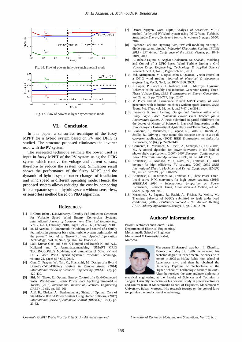
In hypo-synchronous 2 mode, Irradiation was changed from 1 pu to 1.2 pu at t=0.6s and wind speed is decreased from 0.98 pu to 0.94 pu at t=0.8s. Fig. 16 presents that the PV fed the power to the rotor through RSC and the grid through GSC. In hyper-synchronous mode, the rotor and the PV system supplies the grid through the GSC converter (Fig. 17).
Fig. 15. Flow of powers in hypo-synchronous 1 mode
M. El Azzaoui, H. Mahmoudi, K. Boudaraia
Copyright © 2017 Praise Worthy Prize S.r.l. - All rights reserved International Review on Modelling and Simulations, Vol. 10, N. 3
158
Fig. 16. Flow of powers in hypo-synchronous 2 mode
Fig. 17. Flow of powers in hyper-synchronous mode
VI. Conclusion In this paper, a sensorless technique of the fuzzy
MPPT for a hybrid system based on PV and DFIG is studied. The structure proposed eliminates the inverter used with the PV system.
The suggested technique estimate the power used as input in fuzzy MPPT of the PV system using the DFIG system which remove the voltage and current sensors, therefore to reduce the system cost. Simulation result shows the performance of the fuzzy MPPT and the dynamic of hybrid system under changes of irradiation and wind speed in different operating mode. Hence, the proposed system allows reducing the cost by comparing it to a separate system, hybrid system without sensorless, or sensorless method based on P&O algorithm.
References [1] B.Chitti Babu , K.B.Mohanty, ”Doubly-Fed Induction Generator
for Variable Speed Wind Energy Conversion Systems, International Journal of Computer and Electrical Engineering, Vol. 2, No. 1, February, 2010, Pages 1793-8163, February, 2010.
[2] M. El Azzaoui, H. Mahmoudi, ”Modeling and control of a doubly fed induction generator base wind turbine system optimization of the power,” Journal of Theoretical and Applied Information Technology,, Vol 80, No 2, pp 304-314 October 2015.
[3] Lalit Kumar Goel and Sasi K Kottayil and Rajesh K. and A.D. Kulkarni and T. Ananthapadmanabha, ”SMART GRID TECHNOLOGIES Modeling and Simulation of Solar PV and DFIG Based Wind Hybrid System,” Procedia Technology, volume 21, pages 667-675, 2015.
[4] Gan, C., Prayun, W., Tan, C., Shamshiri, M., Design of a Hybrid Diesel/PV/Wind/Battery System in Remote Areas, (2014) International Review of Electrical Engineering (IREE), 9 (2), pp. 420-430.
[5] Siti, M., Tiako, R., Optimal Energy Control of a Grid-Connected Solar Wind-Based Electric Power Plant Applying Time-of-Use Tariffs, (2015) International Review of Electrical Engineering (IREE), 10 (5), pp. 653-661.
[6] Afif, B., Chaker, A., Benhamou, A., Sizing of Optimal Case of Standalone Hybrid Power System Using Homer Software, (2017) International Review of Automatic Control (IREACO), 10 (1), pp. 23-32.
[7] Danvu Nguyen, Goro Fujita, Analysis of sensorless MPPT method for hybrid PVWind system using DFIG Wind Turbines, Sustainable Energy, Grids and Networks, volume 5, pages 50-57, 2016.
[8] Hyeonah Park and Hyosung Kim, ”PV cell modeling on single-diode equivalent circuit,” Industrial Electronics Society, IECON 2013 - 39th Annual Conference of the IEEE, Vienna, pp. 1845-1849, 2013.
[9] A. Babaie Lajimi, S. Asghar Gholamian, M. Shahabi, Modeling and Control of a DFIG-Based Wind Turbine During a Grid Voltage Drop, Engineering, Technology & Applied Science Research, Vol. 1, No. 5, Pages 121-125, 2011.
[10] Md. Arifujjaman, M.T. Iqbal, John E. Quaicoe, Vector control of a DFIG wind turbine, Journal of electrical & electronics engineering, Vol 9, No 2, pp. 1057-1066, 2009.
[11] J. Lopez, P. Sanchis, X. Roboam and L. Marroyo, Dynamic Behavior of the Doubly Fed Induction Generator During Three-Phase Voltage Dips, IEEE Transactions on Energy Conversion, vol. 22, no. 3, pp. 709-717, Sept. 2007.
[12] M. Pucci and M. Cirrincione, Neural MPPT control of wind generators with induction machines without speed sensors, IEEE Trans. Ind. Elec., vol. 58, no. 1, pp.37-47, Jan 2011.
[13] Lawrence Kiprono Letting, Design and Implementation of a Fuzzy Logic Based Maximum Power Point Tracker for a Photovoltaic System, A thesis submitted in partial fulfillment for the degree of Master of Science in Electrical Engineering in the Jomo Kenyatta University of Agriculture and Technology, 2008.
[14] Buonomo, S., Musumeci, S., Pagano, R., Porto, C., Raciti, A., Scollo, R., Driving a mew monolithic cascode device in a dc-dc converter application, (2008) IEEE Transactions on Industrial Electronics, 55 (6), pp. 2439-2449.
[15] Chimento, F., Musumeci, S., Raciti, A., Sapuppo, C., Di Guardo, M., A control algorithm for power converters in the field of photovoltaic applications, (2007) 2007 European Conference on Power Electronics and Applications, EPE, art. no. 4417291, .
[16] Attaianese, C., Monaco, M.D., Nardi, V., Tomasso, G., Dual inverter for high efficiency PV systems, (2009) 2009 IEEE International Electric Machines and Drives Conference, IEMDC '09, art. no. 5075298, pp. 818-825.
[17] Attaianese, C., Di Monaco, M., Tomasso, G., Three-Phase Three-Level active NPC converters for high power systems, (2010) SPEEDAM 2010 - International Symposium on Power Electronics, Electrical Drives, Automation and Motion, art. no. 5542195, pp. 204-209.
[18] Musumeci, S., Pagano, R., Raciti, A., Frisina, F., Melito, M., Transient behavior of IGBTs submitted to fault under load conditions, (2002) Conference Record - IAS Annual Meeting (IEEE Industry Applications Society), 3, pp. 2182-2189.
Authors’ information Power Electronics and Control Team, Department of Electrical Engineering, Mohammadia School of Engineers, Mohammed V University, Rabat, Morocco.
Marouane El Azzaoui was born in Khenifra, Morocco on May 14, 1986, he received his bachelor degree in experimental sciences with honors in 2005 at Molay Rchid high school of Aguelmous city, and then he obtained the University Diploma of Technologie at the Higher School of Technologie Meknes in 2008. After, he received the state engineer diploma in
electrical engineering at the Faculty of Sciences and Technics in Tangier. Currently he continues his doctoral study in power electronics and control team at Mohammadia School of Engineers, Mohammed V University, Rabat, Morocco. His research focuses on the control laws to optimize the production of wind energy.

M. El Azzaoui, H. Mahmoudi, K. Boudaraia
Copyright © 2017 Praise Worthy Prize S.r.l. - All rights reserved International Review on Modelling and Simulations, Vol. 10, N. 3
159
Hassane Mahmoudi was born in Meknes, Morocco, on January 4, 1959. He received B.S degree in electrical engineering from Mohammadia School of Engineers, Rabat, Morocco, in 1982, and the Ph.D degree in power electronic from Montefiore institue of electrical engineering, Luik, Belgium, in 1990. He was an Assistant Professor of physics, at the Faculty of
sciences, Meknes, Morocco, from 1982 to 1990. Since 1992, he has been a Professor at the Mohammadia Schools of engineers, Rabat, Morocco, and he was the Head of Electric Engineering Department during four years (1999, 2000, 2006 and 2007). His research interests include static converters, electrical motor drives, active power filters and the compatibility electromagnetic.
Karima Boudaraia was born in fez Morocco on November 15, 1970. She received her bachelor degree in electronics at Mohamed 5 high school of Benimellal city in 1990; she obtained the Normal High school diploma of Technical education in electrical engineering at Mohammadia in 1996. She is now a teacher of the national diploma in electro-technical higher
education at the Alfaraby Technical High School in Sale. After, she obtained her Applied Higher Education Diploma at Mohammadia School of engineers in 2008. Currently, she pursues her doctoral studies in power electronics and control team at Mohammadia School of engineers, her research focus in the control laws of solar energy.

International Review on Modelling and Simulations (I.RE.MO.S.), Vol. 10, N. 3
ISSN 1974-9821 June 2017
Copyright © 2017 Praise Worthy Prize S.r.l. - All rights reserved https://doi.org/10.15866/iremos.v10i3.11482
160 160 160
Analysis of Flashover Induced by Transient Current During Multiple Lightning Strokes on a Train
Kelvin M. Minja, Pius V. Chombo, Narupon Promvichai, Boonruang Marungsri Abstract – Power system outage due to the occurrence of flashover (across insulators) when lightning induced voltages exceed insulators’ voltage withstand capabilities have been a major investigation in recent studies. Since the Overhead catenary system uses overhead power lines which are exposed to lightning incidences, the concerns have been made in protection against lightning strikes. The knowledge of lightning and its most influential parameters are of great importance in the safe and reliable operation of the Overhead catenary system. In this work, analysis of flashover when lightning strikes on train’s pantograph at the mast and between two masts were studied. Furthermore, the effects of the magnitude, waveforms, polarity, multiplicity and grounding resistance were investigated. In this task, the impact of lightning parameters has been achieved with computer simulation tool (ATPDraw). It was shown that the negative multiple lightning of magnitude - 34 kA and above leads flashover when strikes on pantograph at the mast and between two masts. However, the grounding resistance was recognized to have higher predominance in mast induced voltages when a lightning strike occurs at the mid-span unlike along the mast. Hence, the lightning protection design should consider the multiplicity of negative lightning strokes outcome from the point of hitting. Copyright © 2017 Praise Worthy Prize S.r.l. - All rights reserved. Keywords: Catenary, Multiple Lightning Strokes, Flashover, Grounding Resistance, ATP Draw
Nomenclature Ax Auxiliary line Rt Return line Ct Catenary line X1 S-Rail X2 I-Rail X3 Catenary line with composite insulator X4 Return line with spool insulator X5 Auxiliary line with pin insulator R1 Radius between mast and auxiliary line R2 Radius between mast and return line R3 Radius between mast and catenary line H Height of the mast L1 Vertical distance between auxiliary and return
line L2 Vertical distance between return and catenary
line L3 Distance between catenary line and ground Zaux Impedance of the auxiliary line Zreturn Impedance of the return line Zcatenary Impedance of the catenary line Rf Mast grounding resistance IU International unit
I. Introduction Until now, catenary contact system has become more
useful for feeding traction power to electric vehicle [1]-
[6]. In spite of modernization in the electrified railway system, lightning has been a crucial problem in the overhead catenary system [1]-[2]. Statistically, most of the power system outage caused by transient current characteristics are due to lightning strokes [1], [7]-[9]. A power system failure of the overhead catenary system is triggered by direct lightning strokes to phase conductor, shielding wire and ground in line proximity [1], [10]. However, lightning strokes on phase conductor influence dynamic overvoltages, which can disturb the stability of system to a great extent [9]-[11]. It has been reported that when induced overvoltage overreach insulation withstands capability, lightning flashover across insulators occurs [2]. Many works have been performed to estimate the lightning strokes consequences in the overhead catenary system [1], [3]-[4], [12]-[17].
Catenary contact system is among of elevated railway system that has been affected by lightning incidences in Bangkok, Thailand. It has been reported in [18] lightning magnitude ranges 11-171 kA with a positive polarity which accounts for 5% and -10 to -139 kA with negative polarity is 95% of all flash activities. In addition, [19]-[22] described that negative lightning could associate with multiple strokes per flash. Ref. [19], [21]-[22] showed the reported multiple strokes averaging 3 to 4 strokes per flash with intervals of tens of milliseconds. In recent studies, lightning end results were analyzed when it strikes on the mast, conductors, and traction substation of the overhead catenary system by using different

Kelvin M. Minja, Pius V. Chombo, Narupon Promvichai, Boonruang Marungsri
Copyright © 2017 Praise Worthy Prize S.r.l. - All rights reserved International Review on Modelling and Simulations, Vol. 10, N. 3
161
simulation software [1], [3]-[4], [13]-[14], [16]-[17]. But the analyses from these studies were done in single lightning strokes without regard to the enforcement of multiple lightning strokes. Consequently, it is important to analyze characteristics of transient current during multiple lightning strokes in different waveforms and grounding resistance before establishing lightning protection design.
In this study, the effects of grounding resistance in transient current waveforms of multiple lightning strokes are investigated. The transient conditions are simulated using ATPDraw due to it is the capability for solving the electromagnetic transient problem [3]-[4], [9], [14], [18]-[23]. The characteristics depend on the amplitude of transient current during negative multiple lightning strokes on pantograph are examined.
II. Background A nominal voltage of 25 kV AC-50 Hz is normally
used in the railway traction power system [24]. The conductor arrangement in the double-track overhead catenary system on Thai elevated railway system is shown in Figs. 1-2.
The line of 480 m was accompanied by seven masts with 60 m spacing in the simulation. This line was selected between Phayathai and Rajaprarop (see Fig. 3). The supply voltage was injected at both end points of the line. The negative multiple lightning strokes on train’s pantograph were taken as much concern as it strikes on phase conductor.
The pantograph was considered when it is at the Mast (seventh Mast) for Case 1 as shown in Fig. 1 and at the mid-span of Masts (sixth and seventh Masts) for Case 2 as shown in Fig. 2. The lightning sources were presented by the magnitudes of -34 kA, and -50 kA with 1/30.2 µs, 1.2/50 µs, 2/77.5 µs and 3/75 µs waveforms as in [18]. The elevated poles resistance of 50 Ω and grounding resistances of 5, 10, 20, 30, 40, 50, 70, 80, 90 and 100 Ω were used.
Fig. 1. Lightning strike on train’s pantograph at the Mast
Fig. 2. Lightning strike on train’s pantograph at the mid-span of Masts
Fig. 3. Airport Rail link line in Thailand [25]
III. Catenary Contact System III.1. Railway Transmission Line
The railway transmission line is made up on the double-track elevated railway system whereas masts on the elevated poles have a span of 60 meters (see Figs. 1-2). It comprises of the catenary line, return line, and auxiliary line. A double track consists of rails (S-rail and I-rail) with distributed-parameters along both sides of the impact point. Table I presents details of the railway transmission line on elevated poles [13]. An LCC_8 with JMARTI model as shown in Fig. 4 was used to represent a transmission line in ATPDraw. As reported in [26],[29], it was seen that stray current in the railway transmission line might result in electromagnetic interference and large unbalanced traction load with electricity in the vicinity of the railway system. However, the report in [4] showed that an autotransformer and booster transformer could force the traction current to return through designated return conductors of traction supply in order to reduce stray current. Hence, an autotransformer and booster transformer can ensure restitution of transmission energy to the substation from the train. Therefore, a 1:1 ideal transformer was used to model an autotransformer in ATPDraw. Its modeling details are given in [13]-[14]. In Fig. 5, the cross-section

Kelvin M. Minja, Pius V. Chombo, Narupon Promvichai, Boonruang Marungsri
Copyright © 2017 Praise Worthy Prize S.r.l. - All rights reserved International Review on Modelling and Simulations, Vol. 10, N. 3
162
view of the electrified railway system of a double-track elevated rail system and mast configuration parameters of 2×25 kV AC, 50 Hz from [15] are presented.
TABLE I
DETAILS OF 25 KV TRANSMISSION LINE FOR ELECTRIFIED RAILWAY [2], [13]
Conductors Radius Catenary (X3) 5.06 cm Return (X4) 0.82 cm
Auxiliary (X5) 0.56 cm Ruling span between Masts 60 m
Railway Radius S-rail (X1) 4.95 cm I-rail (X2) 4.95 cm Insulators Impulse Withstand Voltage (MV)
Composite (X3) 0.225 Spool (X4) 0.060 Pin (X5) 0.140
Ground System Grounding resistance 5 - 100 Ω
Elevated Pole Resistance 50 Ω
Fig. 4. Railway Transmission lines data in ATPDraw
Fig. 5. Cross-section view axis of Railway Electrification system on Double Track elevated railway system [15]
III.2. Multiple Lightning Source
Since the disastrous potency of multiple lightning was aimed in the study, some parameters were set in the
ATPDraw models to characterize its behavior. Following the most occurring tendency of negative lightning strokes in Thailand [18], the magnitude of lightning current was considered with a negative polarity.
Although the report of [18] showed the lightning magnitude to range from -10 kA to -139 kA, but only -34 kA and -50 kA were used in this study.
Furthermore, three strokes per flash with intervals of 1ms were used to represent multiplicity as considered in [19], [21]-[22].
The first stroke was modeled with Heidler ideal source at time duration of 0.6 ms; the second and third strokes were designed with two slope Ramp Type 13 at time duration of 0.3 ms for each in ATPDraw. Other parameters of multiple lightning sources are given in Table II.
Fig. 6 illustrates the waveform of the first, second and third strokes of the lightning current with the magnitude of -50 kA.
TABLE II
PARAMETERS OF MULTIPLE LIGHTNING SOURCES [18]-[22]. Parameter Source 1 Source 2 Source 3
Type Heidler 15 Ramp 13 Ramp 13 Amp. (kA) -34/-50 -26/-42 -23/-39
To 0 0 0 A1 0 0 0
T1(s) 0 0.0003 0.0003 TSta (s) 0 0.0016 0.0029 TSto (s) 0.0006 0.0019 0.0032
0 0.5 1.0 1.5 2.0 2.5 3.0 3.5 4.0-50
-40
-30
-20
-10
0
Time (ms)
Cur
rent
(kA
)
-50 kA (1.0/30.2 µs)
Fig. 6. Waveform of the 1st, 2nd and 3rd strokes of the lightning current with the magnitude of -50 kA and waveform of 1.0/30.2 µs
in ATPDraw
III.3. Mast and Insulator
The cylindrical geometric model in single wave impedance was used to represent the mast model. In the literature of [4] and [27], this model was mostly explained to be recommended by IEEE and CIGRE. Hence, this model as given in [4] was taken to represent the mast.
However, the impedances in the catenary, auxiliary, and return lines have an important virtue in the modeling of the mast; therefore, their impedances were estimated from (1) and tabulated in Table III. As seen from (1), R and H are the radii of lines and height of the mast respectively.

Kelvin M. Minja, Pius V. Chombo, Narupon Promvichai, Boonruang Marungsri
Copyright © 2017 Praise Worthy Prize S.r.l. - All rights reserved International Review on Modelling and Simulations, Vol. 10, N. 3
163
Moreover, Fig. 5 depicts the values of R for catenary, auxiliary and return lines. The results of computed impedances from (1) have been summarized in Table III.
In ATPDraw, the mast was designed by using Linezt_1.sup model. With this type, line impedances and their corresponding heights from the ground were assigned to represent the mast.
Three types of insulators used for supporting three lines in the mast are given in Table I. Since in ATPDraw an insulator is represented by a capacitor in parallel with voltage controlled switch [28], the values of withstanding capability to be assigned to the switch for each insulation was taken from Table I.
From [2], composite, pin and spool insulators were shown to have ten, five and one units per insulator respectively. As discussed in [14], the capacitance of 8.8 pF was given for eleven units of a silicone insulator. Then a Switchvc.sup model was used to incorporate the values of voltage withstands capability and capacitances when simulating in ATPDraw:
60 0 5 RZ lncot . arctanH
(1)
where:
Z is the surge impedance; its IU is Ω; R is the equivalent radius of the mast; its IU is m; H is the height of the mast; its IU is m.
TABLE III
MAST MODELED PARAMETERS Location Parameters Auxiliary Zaux = 159.85 Ω, L1= 2.5 m, R1 = 1.12 m, H = 8 m
Return Zreturn = 293.57 Ω, L2 = 0.2 m, R2 = 0.12 m, H = 8 m Catenary Zcatenary = 112.79 Ω, L3= 5.3 m, R3 = 2.5 m, H = 8 m
III.4. Train Model
A three-car train which consists of the pantograph, locomotive transformer, diode bridge rectifier and two DC motors was used to represent the design of an electric locomotive train. The rectifier bridge is represented by the parallel RC elements and the series resistance of the diodes.
A series reactor is connected between the motor and the rectifier bridge in order to smooth the direct current [29].
The system of the electric locomotive train with components mentioned above is shown in Figs.8-9 as presented in [29]-[30]. Since the study is performed when the pantograph of a powertrain is at the mast and the mid-span of masts, Figs. 7-8 show an electric locomotive train positioned across the mast and mid-span respectively.
As shown in Fig. 8, a railway transmission line has a span of 60 meters and 50 Ω resistance of elevated pole. Furthermore, grounding resistances of 5, 10, 20, 30, 40, 50, 70, 80, 90 and 100 Ω were taken to represent different soil profiles.
Fig. 7. An electric locomotive train across the mast
Fig. 8. An electric locomotive train at the mid-span of Masts
IV. Results and Discussion The simulation results of peak mast induced voltages
across the insulators in the auxiliary, return, and catenary lines are shown in Figs. 9-16 for case 1 and Figs. 17-24 for case 2.
5 10 20 30 40 50 60 70 80 90 100-0.6
-0.8
-1.0
-1.2
-1.4
-1.6
-1.8
Grounding Resistance ()
Mas
t Ind
uced
Vol
tage
(MV)
-34 kA (1.0/30.2 s)
Catenary line Return line Auxiliary line
Fig. 9. Mast induced voltages in Case 1 with -34 kA (1.0/30.2 µs)

Kelvin M. Minja, Pius V. Chombo, Narupon Promvichai, Boonruang Marungsri
Copyright © 2017 Praise Worthy Prize S.r.l. - All rights reserved International Review on Modelling and Simulations, Vol. 10, N. 3
164
5 10 20 30 40 50 60 70 80 90 100-0.6
-0.8
-1.0
-1.2
-1.4
-1.6
-1.8
Grounding Resistance ()
Mas
t Ind
uced
Vol
tage
(MV)
-34 kA (1.2/50 s)
Catenary line Return line Auxiliary line
Fig. 10. Mast induced voltages in Case 1 with -34 kA (1.2/50 µs)
5 10 20 30 40 50 60 70 80 90 100-0.6
-0.8
-1.0
-1.2
-1.4
-1.6
Grounding Resistance ()
Mas
t Ind
uced
Vol
tage
(MV)
-34 kA (2.0/77.5 s)
Catenary line Return line Auxiliary line
Fig. 11. Mast induced voltages in Case 1 with -34 kA (2/77.5 µs)
5 10 20 30 40 50 60 70 80 90 100-0.4
-0.6
-0.8
-1.0
-1.2
Grounding Resistance ()
Mas
t Ind
uced
Vol
tage
(MV)
-34 kA (3.0/75 s)
Catenary line Return line Auxiliary line
Fig. 12. Mast induced voltages in Case 1 with -34 kA (3/75 µs)
5 10 20 30 40 50 60 70 80 90 100-1.0
-1.5
-2.0
-2.5
Grounding Resistance ()
Mas
t Ind
uced
Vol
tage
(MV)
-50 kA (1.0/30.2 s)
Catenary line Return line Auxiliary line
Fig. 13. Mast induced voltages in Case 1 with -50 kA (1.0/30.2 µs)
5 10 20 30 40 50 60 70 80 90 100-1.0
-1.5
-2.0
-2.5
Grounding Resistance ()
Mas
t Ind
uced
Vol
tage
(MV)
-50 kA (1.2/50 s)
Catenary line Return line Auxiliary line
Fig. 14. Mast induced voltages in Case 1 with -50 kA (1.2/50 µs)
5 10 20 30 40 50 60 70 80 90 100-1.0
-1.5
-2.0
-2.5
Grounding Resistance ()
Mas
t Ind
uced
Vol
tage
(MV)
-50 kA (2.0/77.5 s)
Catenary line Return line Auxiliary line
Fig. 15. Mast induced voltages in Case 1 with -50 kA (2/77.5 µs)
5 10 20 30 40 50 60 70 80 90 100-0.8
-1.0
-1.2
-1.4
-1.6
-1.8
Grounding Resistance () M
ast I
nduc
ed V
olta
ge (M
V)
-50 kA (3.0/75 s)
Catenary line Auxiliary line Return line
Fig. 16. Mast induced voltages in Case 1 with -50 kA (3/75 µs)
5 10 20 30 40 50 60 70 80 90 100-0.6
-0.8
-1.0
-1.2
-1.4
Grounding Resistance ()
Mas
t Ind
uced
Vol
tage
(MV)
-34 kA (1.0/30.2 s)
Catenary line Return line Auxiliary line
Fig. 17. Mast induced voltages in Case 2 with -34 kA (1.0/30.2 µs)
5 10 20 30 40 50 60 70 80 90 100-0.6
-0.8
-1.0
-1.2
-1.4
Grounding Resistance ()
Mas
t Ind
uced
Vol
tage
(MV)
-34 kA (1.2/50 s)
Catenary line Return line Auxiliary line
Fig. 18. Mast induced voltages in Case 2 with -34 kA (1.2/50 µs)
5 10 20 30 40 50 60 70 80 90 100-0.6
-0.8
-1.0
-1.2
Grounding Resistance ()
Mas
t Ind
uced
Vol
tage
(MV)
-34 kA (2.0/77.5 s)
Catenary line Return line Auxiliary line
Fig. 19. Mast induced voltages in Case 2 with -34 kA (2/77.5 µs)
Kelvin M. Minja, Pius V. Chombo, Narupon Promvichai, Boonruang Marungsri
Copyright © 2017 Praise Worthy Prize S.r.l. - All rights reserved International Review on Modelling and Simulations, Vol. 10, N. 3
165
5 10 20 30 40 50 60 70 80 90 100-0.4
-0.6
-0.8
-1.0
Grounding Resistance ()
Mas
t Ind
uced
Vol
tage
(MV)
-34 kA (3.0/75 s)
Catenary line Return line Auxiliary line
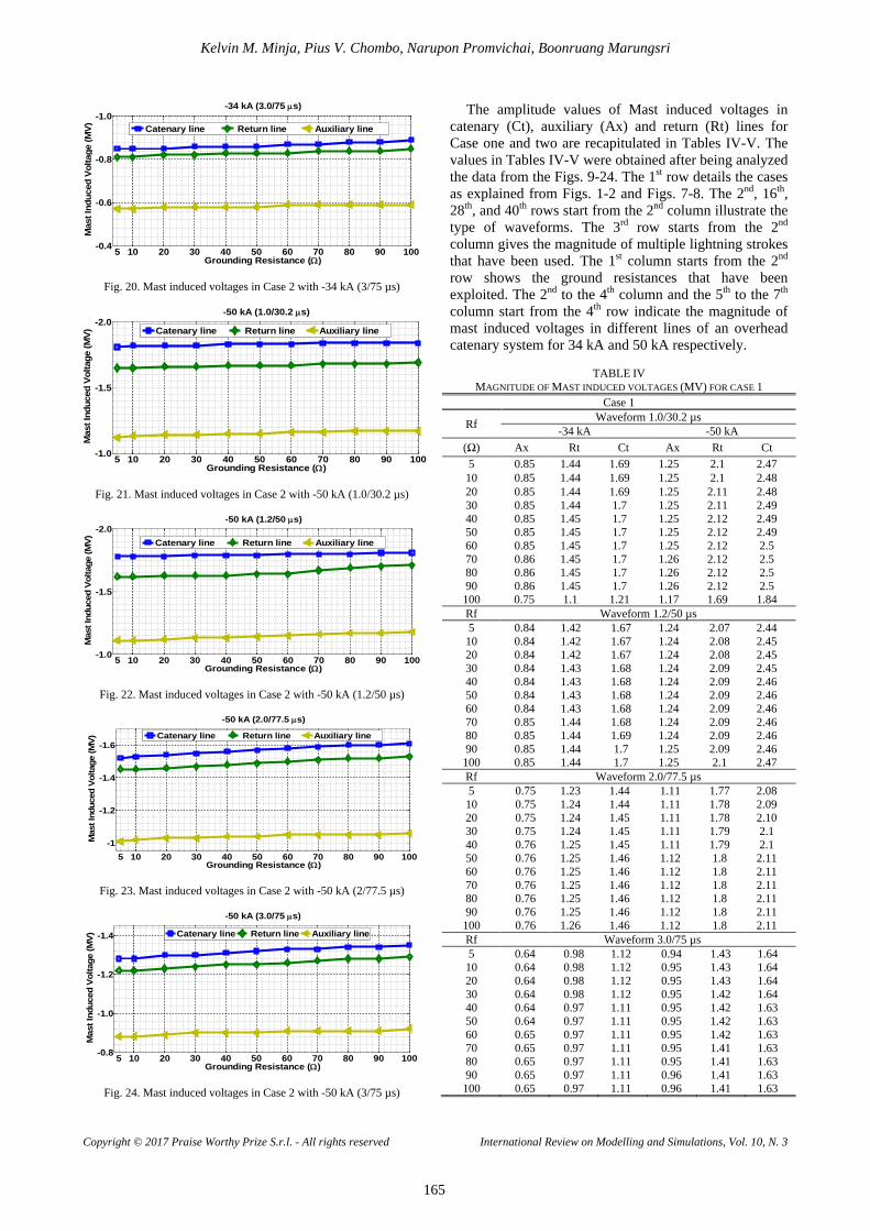
Fig. 20. Mast induced voltages in Case 2 with -34 kA (3/75 µs)
5 10 20 30 40 50 60 70 80 90 100-1.0
-1.5
-2.0
Grounding Resistance ()
Mas
t Ind
uced
Vol
tage
(MV)
-50 kA (1.0/30.2 s)
Catenary line Return line Auxiliary line
Fig. 21. Mast induced voltages in Case 2 with -50 kA (1.0/30.2 µs)
5 10 20 30 40 50 60 70 80 90 100-1.0
-1.5
-2.0
Grounding Resistance ()
Mas
t Ind
uced
Vol
tage
(MV)
-50 kA (1.2/50 s)
Catenary line Return line Auxiliary line
Fig. 22. Mast induced voltages in Case 2 with -50 kA (1.2/50 µs)
5 10 20 30 40 50 60 70 80 90 100-1
-1.2
-1.4
-1.6
Grounding Resistance ()
Mas
t Ind
uced
Vol
tage
(MV)
-50 kA (2.0/77.5 s)
Catenary line Return line Auxiliary line
Fig. 23. Mast induced voltages in Case 2 with -50 kA (2/77.5 µs)
5 10 20 30 40 50 60 70 80 90 100-0.8
-1.0
-1.2
-1.4
Grounding Resistance ()
Mas
t Ind
uced
Vol
tage
(MV)
-50 kA (3.0/75 s)
Catenary line Return line Auxiliary line
Fig. 24. Mast induced voltages in Case 2 with -50 kA (3/75 µs)
The amplitude values of Mast induced voltages in catenary (Ct), auxiliary (Ax) and return (Rt) lines for Case one and two are recapitulated in Tables IV-V. The values in Tables IV-V were obtained after being analyzed the data from the Figs. 9-24. The 1st row details the cases as explained from Figs. 1-2 and Figs. 7-8. The 2nd, 16th, 28th, and 40th rows start from the 2nd column illustrate the type of waveforms. The 3rd row starts from the 2nd column gives the magnitude of multiple lightning strokes that have been used. The 1st column starts from the 2nd row shows the ground resistances that have been exploited. The 2nd to the 4th column and the 5th to the 7th column start from the 4th row indicate the magnitude of mast induced voltages in different lines of an overhead catenary system for 34 kA and 50 kA respectively.
TABLE IV
MAGNITUDE OF MAST INDUCED VOLTAGES (MV) FOR CASE 1 Case 1
Rf Waveform 1.0/30.2 µs -34 kA -50 kA
(Ω) Ax Rt Ct Ax Rt Ct 5 0.85 1.44 1.69 1.25 2.1 2.47
10 0.85 1.44 1.69 1.25 2.1 2.48 20 0.85 1.44 1.69 1.25 2.11 2.48 30 0.85 1.44 1.7 1.25 2.11 2.49 40 0.85 1.45 1.7 1.25 2.12 2.49 50 0.85 1.45 1.7 1.25 2.12 2.49 60 0.85 1.45 1.7 1.25 2.12 2.5 70 0.86 1.45 1.7 1.26 2.12 2.5 80 0.86 1.45 1.7 1.26 2.12 2.5 90 0.86 1.45 1.7 1.26 2.12 2.5 100 0.75 1.1 1.21 1.17 1.69 1.84 Rf Waveform 1.2/50 µs 5 0.84 1.42 1.67 1.24 2.07 2.44
10 0.84 1.42 1.67 1.24 2.08 2.45 20 0.84 1.42 1.67 1.24 2.08 2.45 30 0.84 1.43 1.68 1.24 2.09 2.45 40 0.84 1.43 1.68 1.24 2.09 2.46 50 0.84 1.43 1.68 1.24 2.09 2.46 60 0.84 1.43 1.68 1.24 2.09 2.46 70 0.85 1.44 1.68 1.24 2.09 2.46 80 0.85 1.44 1.69 1.24 2.09 2.46 90 0.85 1.44 1.7 1.25 2.09 2.46 100 0.85 1.44 1.7 1.25 2.1 2.47 Rf Waveform 2.0/77.5 µs 5 0.75 1.23 1.44 1.11 1.77 2.08
10 0.75 1.24 1.44 1.11 1.78 2.09 20 0.75 1.24 1.45 1.11 1.78 2.10 30 0.75 1.24 1.45 1.11 1.79 2.1 40 0.76 1.25 1.45 1.11 1.79 2.1 50 0.76 1.25 1.46 1.12 1.8 2.11 60 0.76 1.25 1.46 1.12 1.8 2.11 70 0.76 1.25 1.46 1.12 1.8 2.11 80 0.76 1.25 1.46 1.12 1.8 2.11 90 0.76 1.25 1.46 1.12 1.8 2.11 100 0.76 1.26 1.46 1.12 1.8 2.11 Rf Waveform 3.0/75 µs 5 0.64 0.98 1.12 0.94 1.43 1.64
10 0.64 0.98 1.12 0.95 1.43 1.64 20 0.64 0.98 1.12 0.95 1.43 1.64 30 0.64 0.98 1.12 0.95 1.42 1.64 40 0.64 0.97 1.11 0.95 1.42 1.63 50 0.64 0.97 1.11 0.95 1.42 1.63 60 0.65 0.97 1.11 0.95 1.42 1.63 70 0.65 0.97 1.11 0.95 1.41 1.63 80 0.65 0.97 1.11 0.95 1.41 1.63 90 0.65 0.97 1.11 0.96 1.41 1.63 100 0.65 0.97 1.11 0.96 1.41 1.63

Kelvin M. Minja, Pius V. Chombo, Narupon Promvichai, Boonruang Marungsri
Copyright © 2017 Praise Worthy Prize S.r.l. - All rights reserved International Review on Modelling and Simulations, Vol. 10, N. 3
166
TABLE V MAGNITUDE OF MAST INDUCED VOLTAGES (MV) FOR CASE 2
Case 2
Rf Waveform 1.0/30.2 µs -34 kA -50 kA
(Ω) Ax Rt Ct Ax Rt Ct 5 0.71 1.09 1.2 1.12 1.65 1.81
10 0.72 1.09 1.2 1.13 1.65 1.82 20 0.72 1.09 1.2 1.14 1.66 1.82 30 0.73 1.09 1.2 1.14 1.66 1.82 40 0.73 1.1 1.2 1.15 1.67 1.83 50 0.73 1.1 1.21 1.15 1.67 1.83 60 0.74 1.1 1.21 1.16 1.67 1.83 70 0.74 1.1 1.21 1.16 1.68 1.84 80 0.74 1.1 1.21 1.17 1.68 1.84 90 0.75 1.1 1.21 1.17 1.68 1.84
100 0.75 1.1 1.21 1.17 1.69 1.84 Rf Waveform 1.2/50 µs 5 0.71 1.07 1.17 1.11 1.62 1.78
10 0.71 1.07 1.17 1.11 1.62 1.78 20 0.71 1.07 1.18 1.12 1.63 1.78 30 0.72 1.07 1.18 1.13 1.63 1.79 40 0.72 1.07 1.18 1.13 1.63 1.79 50 0.72 1.07 1.18 1.14 1.64 1.79 60 0.73 1.08 1.18 1.15 1.64 1.80 70 0.73 1.08 1.18 1.16 1.67 1.80 80 0.73 1.08 1.18 1.17 1.69 1.80 90 0.73 1.08 1.19 1.17 1.7 1.81
100 0.74 1.08 1.19 1.18 1.71 1.81 Rf Waveform 2.0/77.5 µs 5 0.65 0.94 0.99 1.01 1.45 1.52
10 0.65 0.93 0.99 1.02 1.45 1.53 20 0.66 0.95 1 1.03 1.46 1.54 30 0.66 0.96 1.01 1.03 1.47 1.55 40 0.67 0.97 1.02 1.04 1.48 1.56 50 0.67 0.97 1.02 1.04 1.49 1.57 60 0.67 0.98 1.03 1.05 1.5 1.58 70 0.67 0.98 1.03 1.05 1.51 1.59 80 0.68 0.99 1.04 1.05 1.52 1.6 90 0.68 0.99 1.04 1.05 1.52 1.6
100 0.68 0.99 1.05 1.06 1.53 1.61 Rf Waveform 3.0/75 µs 5 0.85 1.44 1.69 1.25 2.1 2.47
10 0.85 1.44 1.69 1.25 2.1 2.48 20 0.85 1.44 1.69 1.25 2.11 2.48 30 0.85 1.44 1.7 1.25 2.11 2.49 40 0.85 1.45 1.7 1.25 2.12 2.49 50 0.85 1.45 1.7 1.25 2.12 2.49 60 0.85 1.45 1.7 1.25 2.12 2.5 70 0.86 1.45 1.7 1.26 2.12 2.5 80 0.86 1.45 1.7 1.26 2.12 2.5 90 0.86 1.45 1.7 1.26 2.12 2.5
100 0.75 1.1 1.21 1.17 1.69 1.84
In the following sections, two different cases are discussed.
IV.1. The Effects of Negative Multiple Lightning Strokes on Train’s Pantograph at the Mast.
Results of mast induced voltages in Case 1 for -34 kA and -50 kA are shown in Figs. 9-16, and summarized in Table IV. It can be noted that the mast induced voltages were above withstand capabilities of line insulators for both catenary, auxiliary, and return lines. Marungsri et al. [18] studied about back flashover affected by tower grounding resistance and concluded that the shorter the waveform, the higher is the tower induced voltages. As seen in Figs. 9-12, it can be clearly observed that the
shortest waveform has the highest mast induced voltages in Catenary, Auxiliary, and Return line as well.
It can also be found that an increase in lightning magnitude from -34 kA to -50 kA resulted into increase in mast induced voltage (see Figs. 9-16). However, flashover was early observed with -34 kA which meant a flashover occurred from -34 kA and above with negative multiple lightning strokes. Furthermore, grounding resistance showed less significance in the performance of multiple lightning. Therefore, when the pantograph is stroke by negative multiple lightning along the mast, flashover was seemed to occur from -34 kA and above, in all waveforms and all grounding resistance. Apart from the occurrence of flashover, the catenary line was appeared to have the highest level of mast induced voltage compared to other lines as shown in Tables IV-V.
IV.2. The Effects of Negative Multiple Lightning Strokes on Train’s Pantograph
at the Mid-Span of Masts
Results of mast induced voltages in Case 2 for -34 kA and -50 kA are given from Figs. 17-24. Table V illustrates the summary of induced voltages in the catenary, auxiliary, and return lines. As depicted in Figs. 17-20, It can be observed that the mast induced voltages are above withstand capabilities of line insulators for both catenary, auxiliary, and return lines. The same results were seen in Figs. 21-24 for -50 kA. Although the effects of lightning magnitude and shorter waveform were also seen as in Case 1 but grounding resistance showed the significant contribution to the flashovers in Case 2. In general, flashover was seemed to occur from -34 kA and above, in all waveforms and all grounding resistance when the pantograph is stroke by negative multiple lightning at the mid-span. Again, the catenary line was seemed to have the highest mast induced voltage amongst the lines (see Table V).
V. Conclusion The following have been summarized for the
conclusion: It is noticed that negative multiple lightning of
magnitude -34 kA and above may cause flashover when strikes the pantograph along the mast or at the mid-span.
The grounding resistance is observed to have a higher influence in mast induced voltages when a lightning stroke occurs at the mid-span compared with along the mast.
All waveforms resulted into flashovers although shorter waveforms displayed more top mast induced voltages. Therefore, negative multiple lightning of any waveform can lead into flashover.
In the case of all lightning magnitudes, waveforms, and grounding resistances, catenary line exhibited higher mast induced voltages. The greatest one

Kelvin M. Minja, Pius V. Chombo, Narupon Promvichai, Boonruang Marungsri
Copyright © 2017 Praise Worthy Prize S.r.l. - All rights reserved International Review on Modelling and Simulations, Vol. 10, N. 3
167
occurred when lightning strokes the pantograph along the mast.
Flashovers have been noticed with multiple strokes from -34kA and above in all waveforms and grounding resistances compared to single strokes in literature, this needs considerable attention in designing insulation and protection systems.
Acknowledgements The authors gratefully appreciate the support of High
Voltage Insulation Technology Laboratory of Suranaree University of Technology, Thailand.
References [1] T. Chmielewski, A. Dziadkowiec, Simulations of Fast Transients
in typical 25 kV a.c. railway power supply system, Seminarium ZASTOSOWANIE KOMPUTERÓW W NAUCE I TECHNICE 2013, Gdańsk, Polska, Vol. 23(No. 36):43-46, 2013.
[2] F. Kiessling, R. Puschmann, A. Schmieder, E. Schneider, 2Ed, Contact Lines for Electrical Railways: Planning - Design - Implementation – Maintenance (Siemens Aktiengesellschaft, Berlin and Murnich, 2009).
[3] S. Pastromas, A. Papamikou, G. Peppas, E. Pyrgioti, Investigation of grounding resistance effect on the MV grid of Hellenic electromotive railway during lightning strikes, 33rd International Conference on Lightning Protection, pp. 1-7, 2016.
[4] Y. Yang, and Y. Zhang, Research on Lightning Protection Simulation of High-speed Railway Catenary Based on ATP-EMTP, Journal of information & Computation Science, Vol. 12(Issue 4):1511-1521, 2015.
[5] Imed, M., Mourad, F., Habib, R., Study and design of a hybrid linear actuator for a railway system, (2010) International Review on Modelling and Simulations (IREMOS), 3 (5), pp. 791-795.
[6] Barrero, R., Hegazy, O., Lataire, P., Coosemans, T., Van Mierlo, J., An accurate multi-train simulation tool for energy recovery evaluation in DC rail networks, (2011) International Review on Modelling and Simulations (IREMOS), 4 (6), pp. 2985-3003.
[7] R. Bhattarai, R. Rashedin, S. Venkatesan, A. Haddad, H. Griffiths, N. Harid, Lightning performance of 275 kV Transmission Lines, 43rd International Universities Power Engineering Conference, pp. 1-5, 2008.
[8] IEEE Std. 1100, IEEE Recommended Practice for Powering and Grounding Electronic Equipment, IEEE Standards, 1999.
[9] P. Lertwanitrot, P. Kettranan, P. Itthisathienkul, A. Ngaopitakkul, Characteristics and Behaviour of Transient Current during Lightning Strikes on Transmission Tower, Proceedings of the International MultiConference of Engineers and Computer Scientists 2015(IMECS 2015), Vol 2, pp. 708-713, Hong Kong, March 2015.
[10] IEEE Std. 1313.2, IEEE Guide for the Application of Insulation Coordination, IEEE Standards, 1999.
[11] P.N. Mikropoulos and T.E. Tsovilis, Estimation of the shielding performance of overhead transmission lines: the effects of lightning attachment model and lightning crest current distribution, IEEE Transactions on Dielectrics and Electrical Insulation, Vol. 19(No. 6):2155-2164, 2012.
[12] H. Lingohr, U. Stahlberg, B. Ritchter, and V. Hinrichsen, Overvoltage protection design for DC railways, Elektrische Bahnen, Vol. 101(No. 7):315-320, 2003.
[13] Ziya Mazloom, Multi-conductor transmission line model for electrified railways: A method for responses of lumped devices, Ph.D. dissertation, KTH Electrical Engineering University, Stockholm, Sweden, 2010.
[14] F. Achouri, I. Achouri, M. Khamliche, Protection of 25 kV Electrified Railway System, 4th International Conference on Electrical Engineering(ICEE), pp. 1-6, 2015.
[15] A. Andreotti, U. D. Martinis, A. Pierno, V. A. Rakov, A New Tool for Lightning Induced Voltage Calculations: CiLIV, General
Assembly and Scientific Symposium (URSI GASS), 2014 XXXIth URSI, pp. 1-4, August 2014.
[16] J. Liu, and M.G. Liu, Improved electro-geometric model for estimating lightning outage rate of catenary, IET Electrical Systems in Transportation, Vol. 2(Issue 1):1-8, 2012.
[17] A.V. Wanjari, Effect of Lightning on the Electrified Transmission Railway System, International Journal of Advance Research in Electrical, Electronics and Instrumentation Engineering, Vol. 3(Issue. 7):10663-10671, 2014.
[18] B. Marungsri, S. Boonpoke, A. Rawangpai, A. Oonsivilai, and C. Kritayakornupong, Study of Tower Grounding Resistance Effected Back Flashover to 500kV Transmission Line in Thailand by using ATP/EMTP, International Journal of Electrical, Computer, Energetic, Electronic and Communication Engineering, Vol. 2(No. 6):1061-1068, 2008.
[19] M.A. Omidiora, M. Lehtonen, Performance of Surge Arrester to Multiple Lightning Strokes on Nearby Distribution Transformer, Proceedings of the 7th WSEAS International Conference on Power Systems, pp. 59-65, Beijing, China, September 2007.
[20] J.A. Martinez-Velasco, and F.C. Aranda, EMTP Implementation of a Monte Carlo Method for Lightning Performance Analysis of Transmission Lines, Ingeniare. Revista chilena de ingeniería, Vol. 16(No. 1):169-180, 2008.
[21] M.A. Omidiora, M. Lehtonen, Simulation of Combined Shield Wire and MOV Protection on Distribution Lines in Severe Lightning Areas, Proceedings of the World Congress on Engineering and Computer Science, San Francisco, USA, October 2007.
[22] J. C. Das, Analysis and control of large-shunt-capacitor-bank switching transients, in IEEE Transactions on Industry Applications, vol. 41, no. 6, pp. 1444-1451, Nov.-Dec. 2005.
[23] Sarajcev, P., Wind farm surge arresters energy capability and risk of failure analysis, (2010) International Review on Modelling and Simulations (IREMOS), 3 (5), pp. 926-937.
[24] IEC 60850, Railway Applications – Supply Voltages of Traction Systems, International Electrotechnical Commission standard, 2014.
[25] UMIASEA, Thailand’s Railway Industry-Overview and Opportunities for Foreigners Businesses, (Thailand: UMI Asia Ltd, 2014, pp. 126-142).
[26] Kalantari, M., Sadeghi, M.J., Farshad, S., Fazel, S.S., Modeling and comparison of traction transformers based on the utilization factor definitions, (2011) International Review on Modelling and Simulations (IREMOS), 4 (1), pp. 342-351.
[27] Y Zhang, W. Sima, and Z. Zhang, Summary of the study of tower models for lightning protection analysis, High Voltage Engineering, Vol. 32(No. 7):93-97, 2006.
[28] A. F. Imece, D. W. Durbak, H. Elahi, S. Kolluri, A. Lux, D. Mader, T. E. McDemott, A. Morched, A. M. Mousa, R. Natarajan, L. Rugeles, and E. Tarasiewicz, Modeling Guidelines for Fast Front Transients, IEEE Transactions on Power Delivery, Vol. 11(No. 1):493-506, January 1996.
[29] A. Zupan, A.T. Teklić, B. Filipović-Grčić, Modeling of 25 kV Electric Railway System for Power Quality Studies, EuroCon 2013.Zagreb, Croatia, pp. 844-849, July 2013.
[30] Mustafa KaragÖz, Analysis of the Pantograph Arcing and Its Effect of the Railway Vehicle, Master Degree dissertation, Middle East Technical University, January 2014.
Authors’ information School of Electrical Engineering, Suranaree University of Technology 111 University Avenue, Nakhon Ratchasima 30000, Thailand.
Kelvin Melckzedeck Minja was born in Tanga, Tanzania in 1989. He completed his B.Eng. Degree in Electrical Engineering in 2015 from Dar es Salaam Institute of Technology. He is currently a master’s degree student in the School of Electrical Engineering, Institute of Engineering at the Suranaree University of Technology, Thailand.

Kelvin M. Minja, Pius V. Chombo, Narupon Promvichai, Boonruang Marungsri
Copyright © 2017 Praise Worthy Prize S.r.l. - All rights reserved International Review on Modelling and Simulations, Vol. 10, N. 3
168
Pius Victor Chombo has obtained his B.Eng. Degree in Electrical Engineering from Dar es Salaam Institute of Technology, Tanzania in 2013.He is now a master’s degree student in the School of Electrical Engineering, the Suranaree University of Technology in Thailand. His interest research topics include High Voltage Systems Design and Monitoring, Laboratory and
System Programming.
Narupon Promvichai has obtained his B.Eng. Degree in the School of Electrical Engineering, the Suranaree University of Technology in Thailand, 2015. He is now a master’s degree student in the School of Electrical Engineering, the Suranaree University of Technology in Thailand.
Boonruang Marungsri was born on 1973 in Nakhon Ratchasima Province, Thailand. He received his B. Eng. in 1996 and M. Eng. in 1999 from Chulalongkorn University, Thailand and D. Eng. in 2006 from Chubu University, Kasugai, Aichi, Japan, all in electrical engineering, respectively. Dr. Marungsri is currently a lecturer in School of Electrical
Engineering, Suranaree University of Technology, Thailand. His areas of interest are electrical power system and high voltage insulation technologies.

International Review on Modelling and Simulations (I.RE.MO.S.), Vol. 10, N. 3
ISSN 1974-9821 June 2017
Copyright © 2017 Praise Worthy Prize S.r.l. - All rights reserved https://doi.org/10.15866/iremos.v10i3.8690
169 169 169
Performance Analysis of a Wind Turbine Based on a Self-Excited Induction Generator (SEIG)
Abdallah Belabbes1, Mohamed Bouhamida1, Allal El Moubarek Bouzid1, Mustapha Benghanem1, Mohamed Della-Krachai1, Mamadou Lamine Doumbia2
Abstract – In this paper, magnetic saturation effect of on the self-excited generator (SEIG) used in the micro-grid system is investigated. The effect of the reduction of the electrical quantities generated voltage and its frequency following a purely resistive or inductive balanced or unbalanced load connection are studied in detail. A dynamic model of SEIG in the fixed reference axis dq is developed and simulated using Simulink / Matlab. The results of the simulations of different scenarios are discussed, and conclusions are deduced at the end of this article. These results will be used to study the stability of a micro-grid under a RT-LAB simulator in the future. Copyright © 2017 Praise Worthy Prize S.r.l. - All rights reserved. Keywords: Renewable Energy, Induction Generator, Islanded Wind, Modeling, Self-Excited
Induction Generator
Nomenclature 푉 ,푉 Stator, Rotor d-axis voltages 퐼 , 퐼 Stator, Rotor d-axis currents 푉 ,푉 Stator, Rotor q-axis voltages 퐼 , 퐼 Stator, Rotor q-axis currents 퐿 Magnetizing Inductance 퐿 , 퐿 Stator, Rotor Inductances 퐼 Magnetizing current 푇 Electromagnetic Torque 푃 Number of poles 푅 ,푅 Stator, Rotor resistance 퐶 Per phase terminal excitation capacitance 푅,퐿 Load Resistance/ Inductance per phase 휔 Angular speeds of Rotor 푉 ,푉 d-q axes load voltage per phase 퐼 , 퐼 d-q axes load current per phase 푉 ,푉 d-q axes capacitor voltage per phase 퐼 , 퐼 d-q axes capacitor currents per phase 푇 Shaft load torque 푋 Multiplier of speed 푃 Mechanical input power 푉 Wind velocity 훽 Blade angle 푅 Radius of the wind turbine 휌 Air density
I. Introduction The gradual increase in oil prices combined with the
hope to reduce oil consumption over the next 50 years have forced researchers to focus their attention to the production of green electricity as an alternative power
source [1]-[22]. Wind is a renewable energy because it is a clean and abundant resource that can generate electricity with virtually no emissions of polluting gases. The application of asynchronous generator is more and more extensive [19]-[22]. Especially, the self-excited asynchronous generator has the advantages of simple structure, high reliability and high-speed operation. The role of independent power system has become increasingly prominent, from the perspective of national defense modernization, the significance of the study of asynchronous generators is particularly important. In fact, asynchronous generators for many years has been a hot topic of scholars [2]-[4].
The self-excited induction generators are good candidates for application in wind turbines in remote areas. Transient operation is an important aspect of asynchronous generator operation. Through the analysis of the transient process of asynchronous generator, it is possible to understand the instantaneous change of the voltage and current when the operating state changes. Asynchronous generator is running, often according to the need to connect/disconnect load. When switching load, the state of the asynchronous generator changes and the transient change in voltage and current during this process is a matter of concern. Many literatures on the asynchronous generator switch the load when the transient process has been analyzed [5], [6]. The specific method is to write a differential process to reflect the transient process and solve the results obtained, these documents only involve the quantitative calculation of the transient process, and the transient operation of the self-excited induction generator connected to the load is not understood from the point of view of the stability of the system.

A. Belabbes et al.
Copyright © 2017 Praise Worthy Prize S.r.l. - All rights reserved International Review on Modelling and Simulations, Vol. 10, N. 3
170
The self-induction generator has non-time-varying non-linearity characteristics after the self-excited operation [7]. The non-linear circuit autonomous state equation theory is used as the starting point for the analysis of the transient process stability of asynchronous generators [8].Based on stability analysis, the fourth order Runge-Kutta method is used to solve the autonomous state equation step by step, the instantaneous values of the state variables in the stationary coordinate system are obtained. Through the conversion from static coordinate system to the actual coordinate system, the instantaneous value of each variable will be draw the corresponding waveform, to reflect the transient process of the current and voltage changes when the asynchronous generator is switched to load [9].
Fig. 1 shows the principle of converting electric energy in a wind turbine. The SEIG has a self-protection mechanism because the voltage collapses when there is a short circuit at its terminals. In addition, SEIGs have other advantages such as low cost, reduced maintenance, brushless construction with the squirrel cage rotor and simple, no DC power required for excitation. The cost of maintenance is low cost compared to the synchronous generator [9], [10]. In this paper, the physical nature of the transient process of the self-excited asynchronous generator and the mathematical law of the corresponding nonlinear autonomous state equation are used to analyze the problem of self-excitation and loads.
Fig. 1. Principle of Wind Energy Conversion
II. Modeling of Wind Turbine II.1. Aerodynamic Model
The aerodynamic model should produce aerodynamic torque from the wind speed and the rotational speed of the turbine. This speed corresponds to the rotational speed of the low speed shaft (훺 ) [11], [12]. To perform modeling of aerodynamics, the expression of mechanical power produced by a wind turbine is used. This quantity of power 푃 depends on the power coefficient 퐶 . It is given by the following equation:
푃 =12휌휋푅 푉 퐶 (휆,훽) (1)
The-power coefficient-is a function-of-the-specific
speed (λ) and-the pitch-angle (β) of-the-blades-of the
wind-turbine. The expression-of-mechanical-power can be-modified to-represent-the-mechanical-torque of the power-extracted-from the wind:
푇 =12휌휋푅 푉
퐶 (휆,훽)훺
(2)
휆 =훺 푅푉
(3)
If β-is fixed, we-have:
푇 =12휌휋푅 푉
퐶 (휆)훺
(4)
The power-coefficient is-generally-modeled by-the
following analytical-expression:
퐶 (휆,훽) = 푐푐휆− 푐 훽 − 푐 푒 + 푐 휆 (5)
휆 =1
휆 + 0.08훽−
0.035훽 + 1
(6)
with 푐 = 0.5176, 푐 = 116, 푐 = 0.4, 푐 = 5, 푐 =21, 푐 = 0.0068
A-typical ratio of 퐶 and 휆 is-shown in-Fig. 2. It is clear from-this figure-that there is a λ value-for which the-power-coefficient (퐶 ) is-maximal [12].
Fig. 2. Power coefficient in function of the specific speed for a fixed pitch (β = 0)
II.2. Wind Speed Gearbox Model
The multiplier adjusts the speed (slow) of the turbine to the generator speed (Fig. 3). This multiplier is mathematically modeled by the following equations:
푇 = 푇 퐺⁄ (7)
훺 =훺퐺
(8)
III. Modeling of SEIG The model used for the simulation of the operation of
the asynchronous machine takes into account the effect
Wind
Turbine Generator Gearbox
Load
Kinetic energy Mechanical energy Electrical energy

A. Belabbes et al.
Copyright © 2017 Praise Worthy Prize S.r.l. - All rights reserved International Review on Modelling and Simulations, Vol. 10, N. 3
171
of saturation of the materials. Indeed, the gap of asynchronous machines is generally low and the nonlinearity of magnetic materials has a significant effect [13], [14].
Fig. 3. Simplified mechanical model of the turbine
This effect is difficult to understand in the case of conventional phase models. Therefore, it usually adopts two-phase models to consider in a comprehensive manner. Of course, this assumes that the induction is homogeneous in the whole structure. In our approach, we adopt the d-q Park model of the asynchronous machine. The effect of saturation is taken into account via a magnetizing inductance (Lm). This is approximated by a polynomial function of the voltage 푉 [14], [15]. Using the relationships between the components of flux and currents in the 푑푞 arbitrary reference benchmark yields the voltage equations and flow expressed as below.
Electrical Equations
For the stator:
푉 = 푅 푖 + 휔휙 + 푝휙푉 = 푅 푖 − 휔휙 + 푝휙 (9)
For the rotor:
푉 = 푅 푖 + (휔 − 휔 )휙 + 푝휙푉 = 푅 푖 − (휔 − 휔 )휙 + 푝휙 (10)
Magnetic Equations
For the stator:
휙 = 퐿 푖 + 퐿 푖 + 푖휙 = 퐿 푖 + 퐿 (푖 + 푖 )
(11)
For the rotor:
휙 = 퐿 푖 + 퐿 푖 + 푖휙 = 퐿 푖 + 퐿 (푖 + 푖 )
(12)
Equation of Electromagnetic Torque:
푇 =32
(푃퐿 ) 푖 푖 − 푖 푖 (13)
Driving Torque of the SEIG:
푇 =퐽푃
푃휔 + 푇 + 푓푃휔 (14)
훺 = 푃 · 휔 (15)
where 휙 , 휙 , 휙 and 휙 denotes the flux linkage, and p denotes the Laplace operator.
The self-excited induction generator (SEIG) works just like an induction machine in the saturation region, except for the fact that there are excitation capacitors connected across the terminals of the stator. In our work, the benchmark reference related to the stator (ω = 0) is used to simulate the model of SEIG (Figs. 4).
Figs. 4. Circuit diagrams of the SEIG in the Park reference d-axis and q-axis connected to the stator
State-space dynamic model of SEIG:
퐼 = 퐴퐼 + 퐵푈 (16)
⎩⎪⎪⎪⎪⎪⎪⎨
⎪⎪⎪⎪⎪⎪⎧
퐼=
⎣⎢⎢⎢⎢⎢⎢⎡푖
푖
푖
푖 ⎦⎥⎥⎥⎥⎥⎥⎤
퐵 =1퐿
⎣⎢⎢⎢⎢⎢⎢⎡퐿 퐾 − 퐿 푉
퐿 퐾 − 퐿 푉
퐿 푉 − 퐿 퐾
퐿 푉 − 퐿 퐾 ⎦⎥⎥⎥⎥⎥⎥⎤
퐴 =1퐿
⎣⎢⎢⎢⎢⎢⎢⎡−퐿 푅 − 퐿 휔 퐿 푅 − 퐿 휔 퐿
퐿 휔 −퐿 푅 퐿 휔 퐿 퐿 푅
퐿 푅 퐿 휔 퐿 −퐿 푅 퐿 휔 퐿
– 퐿 휔 퐿 퐿 푅 −퐿 휔 퐿 −퐿 푅 ⎦⎥⎥⎥⎥⎥⎥⎤ (17)
퐿 = 퐿 + 퐿 and 퐿 = 퐿 + 퐿 (18)
푅 퐿 퐿
퐿 푖 푖 푖
휙 휙
푅
푉 퐶
푠 −휔 휙
+ −
(a) 푅 퐿 퐿
퐿
푖푖 푖 휙 휙
푅
푉 퐶
푠 −휔 휙
+ −
(b)
훺
훺
G 푓
푇
푇

A. Belabbes et al.
Copyright © 2017 Praise Worthy Prize S.r.l. - All rights reserved International Review on Modelling and Simulations, Vol. 10, N. 3
172
The capacitor voltages in Figs. 4 can be represented:
푉 =1퐶
푖 푑푡 + 푉 (19)
푉 =1퐶
푖 푑푡 + 푉 (20)
III.1. Determination of the Initial Conditions
The induction machine requires the residual magnetism for the self-energizing process. Residual magnetism cannot be zero. The initial conditions required in the equation for the simulation of self-excited induction generator can be determined from measurements of the induction machine and capacitors. The initial voltage on the capacitor decreases with time due to leaks. 푉 ,푉 are the initial capacitor voltages:
푉 = 푉 and 푉 = 푉 | (21)
The constants 퐾 and 퐾 are due to the remanent flux in the machine:
퐾 = 휔 휙 and 퐾 = 휔 휙 (22)
III.2. Modeling of an Autonomous Induction Generator Taking Into Account the Saturation
In most cases, the linear model of the asynchronous machine is sufficient to achieve good results in the analysis of transients (start ...). This model assumes that the magnetizing inductance is constant, which is not entirely true, since the magnetic material used for manufacturing is not perfectly linear. However, in certain utilizations of the asynchronous machine (self-excited generator, wind), it is essential to take into account the effect of magnetic circuit saturation and thus the variation of the magnetizing inductance [16], [17]. When the capacitors are connected across the terminals of the stator of an induction machine, driven by an external motor or a wind turbine, a voltage will be induced on its terminals. The electromotive force (EMF) and the current induced in the stator windings will continue to rise until the balanced state is reached, influenced by the magnetic saturation of the machine. Therefore, the magnetizing current should be calculated for each stage of integration in terms of dq currents of the stator and rotor as:
퐼 = (퐼 + 퐼 ) + 퐼 + 퐼 (23)
The magnetizing inductance is calculated from the
magnetization characteristic expressed using the curve between 퐿 and 푉 . The relationship between 퐿 and 푉 is achieved by a synchronous speed test for SEIG testing and can be written as:
퐿 = −1.57 × 10 푉 + 2.44 × 10 푉− 1.19 × 10 푉+ 1.42 × 10 푉 + 0.245
(24)
TABLE I
PARAMETERS OF THE TURBINE Parameters name Values
Wind radius Multiplier Gain Inertia of the shaft Air density
R=35.25 m G = 6 J =100 kg m2
ρ =1.225 kg/m3
TABLE II
PARAMETERS OF THE SEIG Parameters name Values
Nominal power Nominal voltage Nominal current Stator resistance Rotor resistance Stator inductance Rotor inductance Mutual inductance Number of pole pairs Coefficient of friction Frequency
Pm = 3.6 kW Vn=250 V (Δ) In =7.8 A 푅푠=1.66 Ω 푅푟 =2.74 Ω 퐿푠= 11.4 mH 퐿푟= 11.4 mH 퐿m= 180 mH P = 2 푓푟=0.0024N m s-1 f= 50 Hz
IV. Simulation Results Simulation results were determined for the SEIG
without load and under different loads, with the conditions of balanced and unbalanced excitation. The simulations were carried out with MATLAB / Simulink. Residual magnetism in the machine is taken into account in the simulation process, since it is necessary for the self-excitation. The data of this machine are given in Table I and Table II. The performance of this machine has been studied in different conditions, being balanced and unbalanced. Two excitation capacitors are chosen for 퐶 = 퐶 = 60 μF.
Fig. 5. Schematic Diagram of the WECS
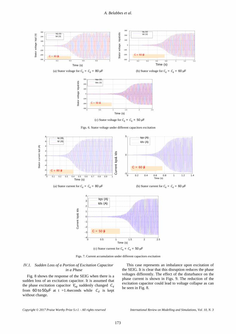
The transient response to different excitation capacitors in Figs. 6 shows the voltage accumulation under different capacitors excitement. It is clear that the process of accumulation is much faster with the larger capacitor (80 μF). In addition, the importance of voltage is much higher in the case of larger capacitor. The effect of the excitation capacitor on the generator current is illustrated in Figs. 7. The excitation current is higher with the larger capacitor excitation.
Induction Generator
Load
Capacitor Bank C
Gear box Wind Turbine
A. Belabbes et al.
Copyright © 2017 Praise Worthy Prize S.r.l. - All rights reserved International Review on Modelling and Simulations, Vol. 10, N. 3
173
(a) Stator voltage for 퐶 = 퐶 = 80 μF (b) Stator voltage for 퐶 = 퐶 = 60 μF
(c) Stator voltage for 퐶 = 퐶 = 50 μF
Figs. 6. Stator voltage under different capacitors excitation
(a) Stator current for 퐶 = 퐶 = 80 μF (b) Stator current for 퐶 = 퐶 = 60 μF
(c) Stator current for 퐶 = 퐶 = 50 μF
Figs. 7. Current accumulation under different capacitors excitation
IV.1. Sudden Loss of a Portion of Excitation Capacitor
in a Phase Fig. 8 shows the response of the SEIG when there is a
sudden loss of an excitation capacitor. It is assumed that the phase excitation capacitor 푉 suddenly changed 퐶푞 from 60 to 50μF at t =1.4seconds while 퐶푑 is kept without change.
This case represents an imbalance upon excitation of the SEIG. It is clear that this disruption reduces the phase voltages differently. The effect of the disturbance on the phase current is shown in Figs. 9. The reduction of the excitation capacitor could lead to voltage collapse as can be seen in Fig. 8.
0 0.5 1 1.5 2 2.5 -4 -3
-2 -1
0 1 2 3 4
Time (s)
Curr
ent Iq
s& Ids
Ids
Iqs (A)
Ids (A)
C = 50 µF
0 0.2 0.4 0.6 0.8 1 1.2 1.4 -5
0
5
Time (s)
Curr
ent Iq
s& Ids
Ids
Iqs (A) Ids (A)
C = 60 µF
0 0.1 0.2 0.3 0.4 0.5 0.6 0.7 0.8 0.9 1 -8 -6 -4 -2 0 2 4 6
8
Time (s)
Sta
tor
curr
ent Iq
d (
A)
(A)
Iq (A) Id (A)
C = 80 µF
0 0.5 1 1.5 2 2.5 -300
-200
-100
0 100 200
300
Time (s)
Sta
tor
volta
ge V
qs&
Vds
Vqs&
Vds
Vqs (V) Vds (V)
C = 50 µF
0 0.2 0.4 0.6 0.8 1 1.2 1.4-300 -200 -100
0 100 200
300
Time (s)
Sta
tor
volta
ge
Vqs&
Vds
Vqs&
Vds
Vq (V)Vd (V)
C = 60 µF 0 0.2 0.4 0.6 0.8 1 -300
-200
-100
0 100 200 300
Time (s)
Sta
tor
volta
ge V
qd (
V)
(V)
Vq (V) Vd (V)
C = 80 µF

A. Belabbes et al.
Copyright © 2017 Praise Worthy Prize S.r.l. - All rights reserved International Review on Modelling and Simulations, Vol. 10, N. 3
174
Fig. 8. Voltage curve with a loss of part of the excitation capacitor
(a) Stator current Iq
(b) Stator current Id
Figs. 9. Current curve with a loss of a part
of the excitation capacitor
IV.2. Simulation of Self-Priming in a Resistive Load
The principle is the same as in case with no load, except that the additional equations will change as follows:
⎩⎪⎨
⎪⎧푖 = 푖 − 푖푑푉푑푡
=1퐶푖
푖 =푉푅
(25)
where 푖 : load current. The effect of the sudden change by a resistive load is shown in Figs. 10, 11. At 푡 = 1.4
seconds the resistive load of 50Ω value is suddenly appliedacross each phase. It is observed that the voltage drop and current increases with an increase against Fig. 12 load current.
Fig. 10. Voltage curve with a resistive load R
Fig. 11. Current curve with a resistive load R
Fig. 12. Current curve of the resistive load R
Fig. 13. Voltage curve for resistive load R=20Ω
0 0.5 1 1.5 2 2.5 -300
-200
-100
0
100
200
300
Time (s)
Volta
ge V
qs&
Vds
Vqs (V)
Vds (V)
t =1.4 R=20 Ohm
0 0.5 1 1.5 2 2.5 -5
0
5
Time (s)
Load
curr
ent (A
)
(A)
Ich (A)
Ich = 0 for R=0
Ich = 4.7A for R=50
0 0.5 1 1.5 2 2.5 -10
-5
0
5
10
Time (s)
Curr
ent Iq
s& Ids
Ids
Iq (A)
Id (A)
t =1.4 s R=50 Ohm
0 0.5 1 1.5 2 2.5 -300 -200
-100 0
100
200 300
Time (s)
Sta
tor
volta
ge V
qs&
Vds
Vqs (V) Vds (V)
t =1.4 R=50 Ohm
0 0.5 1 1.5 2 2.5 -8 -6 -4 -2
0 2 4 6
Time (s)
Sta
tor
curr
ent Id
s (A
)
(A)
Ids
t =1.4 Cq= 20 µF
0 0.5 1 1.5 2 2.5 -5
0
5
Sta
tor
curr
ent Iq
(A)
Iq(A
)
Time (s)
at t=1.4 s Cq = 20 µF
0 0.5 1 1.5 2 2.5 -300
-200
-100
0
100
200
300
Time (s)
Sta
tor
volta
ge V
qs&
Vds
Vqs&
Vds
Vq (V) Vd (V)
t =1.4 Cq= 20 µF

A. Belabbes et al.
Copyright © 2017 Praise Worthy Prize S.r.l. - All rights reserved International Review on Modelling and Simulations, Vol. 10, N. 3
175
But when applying a load 푅 = 20Ω it is seen on Fig. 13 and Fig. 14 that the SEIG peaks and the excitation capacitor cannot have the means for balanced operation and the generator loses its voltage.
Fig. 14. Current curve for resistive load R = 20Ω
IV.3. Simulation of Self-Priming with an Inductive Load
The principle of self-priming charge remains the same as no load, except that the equations of excitement will take another form. The equations in the generalized reference Park transform are:
⎩⎨
⎧푑푑푡푉 =
1퐶
(푖 − 푖 )
푑푑푡푖 =
1퐿
(푉 − 푅 푖 ) (26)
⎩⎨
⎧푑푑푡푉 =
1퐶
푖 − 푖
푑푑푡푖 =
1퐿
푉 − 푅 푖 (27)
The effect of the sudden change caused by RL load is
shown in Figs. 15, 16. At 푡 = 1.4 seconds where 푅 = 50Ω and 퐿 = 5 mH is suddenly applied across each phase.
It is observed that the voltage drop (Fig. 15) and load’s current increases (Fig. 16 and Fig. 17).
Fig. 15. Voltage curve for RL load
Fig. 16. Current curve for RL load
Fig. 17. Current curve of the RL load
The effect of apureinductive loadon transient response is seen in Fig. 18 and Fig. 19, when a sudden pure inductive load is applied at 푡 = 1.4 seconds.
Fig. 18. Voltage curve for purely inductive load
Fig. 19. Current curve for purely inductive load
0 0.5 1 1.5 2 2.5 -5
0
5
Time (s)
Curr
ent Id
s &Iq
s
&Iq
s
Iqs (A)
Ids (A)
L=250 mH
0 0.5 1 1.5 2 2.5 -300
-200
-100
0
100
200
300
Time (s)
Volta
ge V
qs&
Vds
Vqs (V) Vds (V)
L=250 mH
0 0.5 1 1.5 2 2.5 -5
0
5
Load
curr
ent RL
RL
Time (s)
Iload (A)
R=50ohm, L=5 mH
0 0.5 1 1.5 2 2.5 -10
-5
0
5
10
Time (s)
Curr
ent Id
s &Iq
s
&Iq
s
Iqs (A)
Ids (A)
R=50 Ohm L=5 mH
0 0.5 1 1.5 2 2.5 -300
-200
-100
0
100
200
300
Time (s)
Volta
ge V
qs&
Vds
Vqs (V) Vds (V)
R=50 Ohm L=5 mH
0 0.5 1 1.5 2 2.5 -15
-10
-5
0
5
10
15
Time (s)
Curr
ent Iq
s& Ids
Ids
Iqs (A)
Ids (A)
t =1.4 R=20 Ohm

A. Belabbes et al.
Copyright © 2017 Praise Worthy Prize S.r.l. - All rights reserved International Review on Modelling and Simulations, Vol. 10, N. 3
176
The inductor value applied through each phase is 250 mH. The response indicates that the excitation capacitors are not in this case able to keep a stable operation.
V. Conclusion This work presents the development of an overall
dynamic model for a SEIG. The model is suitable for studying the generator operation in balanced and unbalanced conditions as well as operating for different values of the excitation capacitors. Several simulation scenarios were studied and analyzed. The results shown that an SEIG can be efficient, and inexpensive, as a generator for isolated networks system for specific load margin (value and unbalance). Based on the results in [18], this model will be used to study the effects of installing an active filter in an isolated network. This work will be done on a real time simulator.
References [1] B. Multon, O. Gergaud, H. B. Ahmed, X. Roboam, S. Astier, B.
Dakyo, et al., "Etat de l’art dans les aérogénérateurs électriques," Rapport de sysnthèse: l’électronique de puissance vecteur d’optimisation pour les énergies renouvelables», Club Electronique de Puissance, 2002.
[2] R. Bansal, T. Bhatti, and D. Kothari, "Bibliography on the application of induction generators in nonconventional energy systems," IEEE Transactions on Energy Conversion, vol. 18, pp. 433-439, 2003.
[3] R. Bansal, "Three-phase self-excited induction generators: an overview," IEEE transactions on energy conversion, vol. 20, pp. 292-299, 2005.
[4] M. G. Simoes and F. A. Farret, Alternative energy systems: design and analysis with induction generators vol. 13: CRC press, 2011.
[5] M. Salama and P. Holmes, "Transient and steady-state load performance of a stand-alone self-excited induction generator," IEE Proceedings-Electric Power Applications, vol. 143, pp. 50-58, 1996.
[6] L. Wang and J.-Y. Su, "Dynamic performances of an isolated self-excited induction generator under various loading conditions," IEEE Transactions on Energy conversion, vol. 14, pp. 93-100, 1999.
[7] L. S. Singh, CS Jha, Bhim, "Transient analysis of self-excited induction generator supplying dynamic load," Electric Machines &Power Systems, vol. 27, pp. 941-954, 1999.
[8] P. C. Krause, O. Wasynczuk, S. D. Sudhoff, and S. Pekarek, Analysis of electric machinery and drive systems vol. 75: John Wiley & Sons, 2013.
[9] J.-F. Yhuel, "Commande en courant des machines à courant alternatif," ANRT [diff.], 2001.
[10] A. M. Bouzid, A. Cheriti, P. Sicard, M. Bouhamida, and M. Benghanem, "State space modeling and performance analysis of self-excited induction generators for wind simulation," in Control, Engineering & Information Technology (CEIT), 2015 3rd International Conference on, 2015, pp. 1-6.
[11] B. EL Moubarek, "Régulation de la tension d'une génératrice asynchrone auto excitée en utilisant un compensateur statique d'énergie réactive," Ecole Nationale Polytechnique d'Oran, 2012.
[12] D. Guérette, Asservissement d'une éolienne à vitesse variable et à pas fixe dans le cadre d'un système de jumelage éolien-diesel à haute pénétration: Université du Québec à Rimouski, 2010.
[13] C. Grantham and D. Seyoum, "The dynamic characteristics of an isolated self-excited induction generator driven by a wind turbine," in Electrical Machines and Systems, 2008. ICEMS 2008. International Conference on, 2008, pp. 2351-2356.
[14] D. Seyoum, C. Grantham, and M. F. Rahman, "The dynamic
characteristics of an isolated self-excited induction generator driven by a wind turbine," Industry Applications, IEEE Transactions on, vol. 39, pp. 936-944, 2003.
[15] M. S. Abdoulaziz, "Etude du Générateur Asynchrone pour l’utilisation dans la production de l’énergie éolienne," Mémoire d'ingénieure Ecole Nationale Polytechnique d’Alger, 2007.
[16] A. M. Bouzid, P. Sicard, A. Cheriti, J. M. Guerrero, M. Bouhamida, and M. S. Golsorkhi, "Voltage and frequency control of wind-powered islanded microgrids based on induction generator and STATCOM," in Control, Engineering & Information Technology (CEIT), 2015 3rd International Conference on, 2015, pp. 1-6.
[17] D. Lubineau, "Commande non linéaire de moteur asynchrone avec observateur," 1999.
[18] A. Bouzid, A. Cheriti, M. Bouhamida, and M. Benghanem, "Alleviation of harmonics for the self excited induction generator (SEIG) using shunt active power filter," American Journal of Electrical Power and Energy Systems, vol. 2, pp. 81-87, 2013.
[19] Benbouzid, M., Muyeen, S., Khoucha, F., An Up-to-Date Review of Low-Voltage Ride-Through Techniques for Doubly-Fed Induction Generator-Based Wind Turbines, (2015) International Journal on Energy Conversion (IRECON), 3 (1), pp. 1-9.
[20] Ahmed, I., Zobaa, A., Comparative Power Quality Study of Variable Speed Wind Turbines, (2016) International Journal on Energy Conversion (IRECON), 4 (4), pp. 97-104.
[21] Ajewole, T., Lawal, M., Omoigui, M., Development of a Lab-Demo Facility for Wind Energy Conversion Systems, (2016) International Journal on Energy Conversion (IRECON), 4 (1), pp. 1-6.
[22] Barara, M., Chimezie, A., Al Sayari, N., Beig, A., Al Hosani, K., Abbou, A., Akherraz, M., Hardware Implementation of Voltage Control for Self Excited Induction Generator Used in Small Power Generation, (2015) International Review of Electrical Engineering (IREE), 10 (4), pp. 553-560.
Authors’ information 1AVCIS laboratory members, University Mohamed Boudiaf USTO 1505BPEl Mnaouer, Oran 31000, Algeria. E-mails: [email protected]
2Department of Electrical and Computer Engineering, Université du Québec à Trois-Rivières, QC, Canada Trois-Rivières, CANADA.

International Review on Modelling and Simulations (I.RE.MO.S.), Vol. 10, N. 3
ISSN 1974-9821 June 2017
Copyright © 2017 Praise Worthy Prize S.r.l. - All rights reserved https://doi.org/10.15866/iremos.v10i3.11349
177 177 177
Seawater Desalination Pilot Plant: Optimal Design and Sizing of Solar Driven-Four Effect Evaporators
Combined with Heat Integration Analysis
M. Ghazi1,2, E. Essadiqi1, M. Mada2, M. Faqir1, A. Benabdellah1
Abstract – This paper puts forward the results and methodology used for thermal analysis, sizing and design of four effects pilot scale desalination unit combined with solar thermal energy and using falling film evaporators for a production capacity of 7m3/day. The modelling equations are given at steady-state conditions and are based on mass and heat balances equations, heat transfer equations, and thermodynamic and physical properties of each stream. MATLAB programming is used for the resolution of the developed algorithm. The impact of the important parameters, such as evaporator type, tube dimensions, heating medium and top brine temperatures on the performance ratio and heat transfer rate, has been studied. Besides, this work is completed by Pinch analysis to provide the optimal Heat Exchanger Network (HEN) taking into account three different configurations and the impact of the minimum temperature difference ∆Tmin. Results show that it is beneficial to use the horizontal falling film evaporators allowing high heat transfer coefficient values ranging between 3.18 and 3.32kW/m2/K. In addition, the optimal HEN enables a 62% reduction of thermal power needed to feed seawater heating. Also, in this study, several suggestions and criteria for evaporators and HEN design and optimization have also been dealt with. Copyright © 2017 Praise Worthy Prize S.r.l. - All rights reserved. Keywords: Seawater Desalination, MED, Solar Energy, Heat Integration, Pinch Analysis
Nomenclature Ai Heat transfer area for effect i (m2) Bi Partial mass flow rate of rejected brine for
effect i (kg/s) Di Partial mass flow rate of produced fresh water
for effect i(kg/s) Fi Partial mass flow rate of feed seawater for
effect i (kg/s) Vi Mass flow rate of vapor (kg/s) Mb Global flow rate of rejected brine (kg/s) Md Global flow rate of produced fresh water (kg/s) Mf Global flow rate of feed seawater (kg/s) Ms Mass flow rate of heating medium (kg/s) Mcw Mass flow rate of cooling water (kg/s) Q Thermal power (kW) T Temperature (°C) Ti Temperature inside effect i (°C) Ui Overall heat transfer coefficient for effect i
(kW/m2/°C) Nt Number of tubes LMTD Logarithmic mean temperature difference(°C) cp Specific thermal capacity (kJ/kg/°C) Nu Nusselt number Re Reynolds number Pr Prendlt number L Length of tubes (m) λ, Li Latent heat of evaporation/condensation (kJ/kg)
BPE Boiling point elevation (°C) De Equivalent diameter (m) kw Thermal conductivity of metal μ Dynamic viscosity (kg/m/s) ρ Density (kg/m3) η Efficiency (%)
I. Introduction No one can deny that fresh water is one of the most
vital elements for human life. Yet, its shortage has become one of the most serious problems mankind is facing for the few last decades, in many countries in arid and semi-arid areas including Morocco. The use of renewable energy as a heating source for fresh water production by desalination is, therefore, among the most effective ways to tackle both water scarcity and pollution risks [1]-[39].
The high thermal heat consumption is the main problem in seawater desalination when the phase change processes, such as the multi effect evaporation process and Multi stage flash processes are used. This problem becomes more hazardous when renewable energy is used to provide the required thermal energy to the desalination unit because it is difficult to produce the sufficient amount of heat which is equivalent to that produced by traditional fossil fuels. That is why the decrease in energy consumption has been the focus of several research and

M. Ghazi, E. Essadiqi, M. Mada, M. Faqir, A. Benabdellah
Copyright © 2017 Praise Worthy Prize S.r.l. - All rights reserved International Review on Modelling and Simulations, Vol. 10, N. 3
178
engineering studies. Increasing the number of effects in distillation processes is considered as the best solution to decrease the required thermal energy. What is more, the process heat integration can also bring significant reduction of required thermal heat and economic benefits to desalination unit especially for parallel feed MED process by improving the heat exchangers network used for heat recovery. MED desalination process is not a new concept; it is a technology dated back to before the Second World War when desalination systems were based on evaporation processes, as those employed in boats. Around 1930, Small MED units were constructed in the City of Jeddah, Saudi Arabia and in Curacao and Aruba, Netherland Antilles. They were composed of two and three-effect evaporators [1]. In the literature, research on MED desalination process has gained more interest, especially in the last decades. Indeed, there have been many published papers related to modelling, designing and thermal analysis of MED seawater desalination units. Al-Mutaz and Wazeer [2] developed a simple mathematical model for MED-TVC desalination plants in steady-state conditions; they considered all aspects of design procedures for an MED-TVC system, using MATLAB software to evaluate the system performance obtained in terms of gain ratio, specific heat transfer area, specific heat consumption and distillate production. Good agreement has been obtained between model data and actual data when the model validity was tested against some available data of six commercial plants. El-Dessouky et al. [3] presented an efficient mathematical model describing the Multiple Effect Distillation desalination system. The model assumed the case of constant heat transfer areas for the evaporators and the feed pre-heaters in all effects, and the algorithm is implemented using L-A-S computer aided language. The results show that the heat transfer coefficients in the evaporators and the pre-heaters increased with boiling temperature. The heat transfer coefficients in the evaporator are always high when they are compared to that in the pre-heater at the same boiling temperature, while the plant thermal performance ratio is nearly independent of the top brine temperature and strongly related to the number of effects. Khademi et al. [5] described a steady-state simulation and optimization of a six-effect evaporator; they presented the effect of different parameters on consumed steam produced distilled water and GOR. The feed mass flow rate, condenser pressure and operating time are optimized for this system. The simulation shows that the feed temperature plays the most important role in the evaporation plant. Shakib et al. [6] presented a thermodynamic model for ME-TVC combined with gas turbine power using a heat recovery steam generator. They performed an optimization with three approaches: the first approach is a global optimization problem, the second one is a local optimization approach, while the third approach is a multi-objective optimization. El-Dessouk, Ettouney, and Mandani [7] performed a steady state analysis of various configurations of MEE
desalination plant, the results showed that the best performance is obtained from the parallel/cross flow and the parallel flow systems, and operation of both systems is favored at higher temperatures. Moreover, the design, construction, and operation of parallel flow system is simpler. The comparison of the MSF, forward feed, parallel, and parallel-cross flow MEE systems show that the forward feed MEE presents more advantages than the other systems. Palenzuela et al. [8] also carried out a MEE model under steady-state conditions taking into account the same characteristics of the pilot MEE plant at PSA. MATLAB software is used to solve the mathematical model. The model has been validated by comparing it to experimental data from real plant operation; the results show that the errors are lower than 9%. Al-Mutaz et al. [9] developed a mathematical model for the parallel/cross, forward and backward feed configurations; it was found that steam temperature has the major impact on the specific heat transfer area in MEE process and the parallel-cross feed scheme has better performance characteristics than the other two feed configurations.
The combination using renewable energy and MED seawater desalination process has received significant attention by many researchers, especially when solar thermal energy is used. Several publications focus on the modelling, simulation and analysis of MEE desalination process using solar energy are available in the literature. Yılmaz and Söylemez [10] present a design and a mathematical modelling of multi-effect evaporation seawater desalination system with Forward-Feed configuration using hybrid renewable energy sources. Visual Basic programming language is used for computer simulation. The results obtained show a good accordance with data from the literature. Ali M. El-Nashar et al. [11-16] designed and analyzed performances of a seawater solar desalination MES plant, using evacuated tube flat plate collector. The plant was designed for a maximum capacity of 120 m3/day. Bataineh [17] studied the annual performance of multi-effect desalination plant combined with a thermo-compressor MED–TC driven by a solar steam generation using parabolic trough solar collector field. The unit is designed for a production capacity of 50,000 m3/day of fresh water regularly.
In order to innovate or enhance the experimental analysis and results of combining the use of renewable energy and seawater desalination processes, the International University of Rabat proposed the construction of new solar driven seawater desalination pilot scale unit using multi-effect distillation (MED) process. The principal benefits of such a system will be associated with the environment protection, low maintenance and accessibility to small communities. This paper presents the basics and results that are used for the evaporators and heat exchanger networks design, sizing and optimization based on thermal analysis and process heat integration. It is composed of two complementary parts, the first one contains the MED unit sizing based on modelling and simulation under different geometrical

M. Ghazi, E. Essadiqi, M. Mada, M. Faqir, A. Benabdellah
Copyright © 2017 Praise Worthy Prize S.r.l. - All rights reserved International Review on Modelling and Simulations, Vol. 10, N. 3
179
conditions such as evaporators’ tubes dimensions and operating conditions. The second one deals with the heat exchanger network selection and sizing based on Pinch analysis.
II. Process Description and Material Selection
The seawater desalination pilot unit is based on using the multi effect evaporation technology using four effects and solar thermal panels as a source of the required energy. The unit will be installed at the International University of Rabat (UIR-Morocco) with a production capacity of 7 m3/day. As shown in Fig. 1, the unit is composed of three subsystems: The evaporation /condensation unit Heat exchangers network: And solar system
The evaporation/condensation unit is composed of four evaporators assembled using parallel feed configuration. This configuration has been chosen because it is the most economical and more efficient when the feed seawater is nearly saturated, when introduced inside the evaporators [2]. The solar panels are vacuum tubes collector type and they use hot water as a heating medium and, thus, provides the evaporation unit with the required thermal energy.
The required thermal energy for feed seawater heating will be provided by the same source of heat and by the heat recovered from rejected brine and distillate by using the exchanger network.
It is very important to choose appropriate material to ensure proper operation so as to avoid as many problems as possible and thus ensure the plant efficiency. The choice of the suitable type of evaporators and heat exchangers to be used depends on several parameters, essentially: cost, heat transfer rate, maintenance and cleaning and corrosion risks. The most suitable type of evaporator for seawater desalination is the falling film evaporator type. It has two main configurations that include horizontal and vertical tube as shown in Figs. 2. The horizontal tube is the most common design used in the desalination industry because of its significant advantages, such as high heat transfer coefficients under low flow rate and small temperature difference [5]. In this study, both types of falling film evaporators are taken into account in order to make the best choice based on their performances.
It was reported that the recommended material for effect tubing is Aluminum for horizontal tube design and Aluminum brass or copper-nickel for vertical tube design [31]. The Plate heat exchanger type is selected for this plant because of its high heat transfer rate under small temperature difference and ease of maintenance.
The data used in the calculations and design are given in Table I.
Fig. 1. Four effect MED seawater desalination pilot unit

M. Ghazi, E. Essadiqi, M. Mada, M. Faqir, A. Benabdellah
Copyright © 2017 Praise Worthy Prize S.r.l. - All rights reserved International Review on Modelling and Simulations, Vol. 10, N. 3
180
(a) (b)
Figs. 2. (a): Horizontal tubes falling film evaporator, (b): Vertical tubes falling film evaporator
TABLE I
DESIGN DATA OF THE PLANT Solar Panels MED System
Type of panel Vacuum tubes Number of effects 4
K1 and K2 respectively
1,936 W/m2/K 0,006 W/m2/K2
Produced fresh water
mass flow rate
7 m3/day (Day=8houres)
Optical efficiency η0
0,774 Evaporation rate (% of
mass) 25
Solar radiation (Rabat-
Morocco)
800 W/m2
(DNI) Evaporator
type Falling film evaporator
SF 60% Tubes material
Aluminium or Aluminium
brass Absorber area per panel (30
tube) 4,889 m2 Tube
dimensions “Variables”
External dimensions 2,170×2,250 m Seawater
salinity 35 g/l
III. Modelling Equations The modeling of the study state operation of the unit is
carried out based on the mass and energy conservation equations, heat transfer and thermodynamics correlations. The latters are used to estimate the heat transfer coefficients and the thermodynamics properties, such as thermal capacity, viscosity and density of different streams. The resolution of the obtained model is done using an iterative algorithm and Matlab programming software.
This study takes into account the impact of design parameters, including the evaporators’ tubes diameter and length in addition to the operating parameters such as the top brine and heating medium temperatures on the unit performance. The model also considers the following assumptions: Salt concentration equals zero for produced distillated
water; All the evaporators and the condenser are assumed
adiabatic
Steams entering or leaving the evaporators are saturated
Solar irradiation is assumed constant.
III.1. Heat and Mass Balances
III.1.1. Solar System
The thermal power provided by the solar panels depends on the absorber area, the panel efficiency and the solar direct normal irradiation, which is calculated using the following equation:
푃 = 휂퐴 퐸 (1)
The solar efficiency represents the ratio between the
amount of solar irradiation received by the collector and the energy converted into useful heat; it depends on the panel characteristics such as the optical efficiency of the collector transparent glass. The collector efficiency is calculated by [18]:
휂 = 휂 −퐾 ∆푇′퐸
−퐾 (∆푇′)
퐸 (2)
The solar energy is converted into thermal energy and
transferred to heating medium. The energy balance equation for the heating medium is given by the following equation:
푀 푐 (푇 − 푇 ) = 푃 − 푃 (3)
where Ploss is the lost thermal power to the ambient by heat transfer through the piping system.
III.1.2. Evaporators
III.1.2.1. The First Effect
The mass balance equation for the first evaporator is given by:

M. Ghazi, E. Essadiqi, M. Mada, M. Faqir, A. Benabdellah
Copyright © 2017 Praise Worthy Prize S.r.l. - All rights reserved International Review on Modelling and Simulations, Vol. 10, N. 3
181
퐹 = 퐵 + 퐷 (4) The thermal power of the heating medium is used to
evaporate a portion of the feed seawater, thus, the energy balance equation is expressed by the following equation:
푀 푐 (푇 − 푇 ) = 퐷 퐿 + 푃 , (5)
where, the mass flow rate of produced distillated water is obtained by:
퐷 = 푋 퐹 (6)
The required heat transfer area for the evaporator is
related to the power exchanged, the overall heat transfer coefficient and the log mean temperature difference using the following relationship:
푀 푐 (푇 − 푇 ) = 휂 푈 퐴 (퐿푀푇퐷) (7)
where, the LMTD is defined as:
퐿푀푇퐷 = (푇 − 푇 )푙푛 (푇 − 푇푇 − 푇
) (8)
III.1.2.2. Effect 2, 3, and 4
The mass balance equations obtained for the other effects are similar to the first one; indeed, they are given in the following expressions:
퐹 = 퐵 + 퐷 (9)
where:
퐷 = 푋 퐹 (10)
The heat balance equation is given by:
퐷 퐿 = 퐷 퐿 + 푃 , (11) The heat transfer equation is given by:
퐷 퐿 = 휂 푈 퐴 ∆푇 (12)
where, ∆Ti is the temperature difference between the condensing vapor and the boiling seawater.
III.1.3. Last Condenser
An additional mass flow rate of cooling seawater Mcw is added to the condenser to ensure the total condensation of vapor; in this case the last effect vapor’s latent heat of condensation is absorbed by the cooling water and feed seawater. The energy balance equation for the condenser is given by:
푉 퐿 = 푀 + 푀 퐶 푇 − 푇 + 푃 , (13)
The condenser heat transfer equation is expressed by the following:
푉 퐿 = 휂 푈 퐴 (퐿푀퐷푇) (14)
III.2. Heat Transfer Correlations
The global heat transfer coefficient based on the outer surface of the tube is expressed by the following equation:
1푈
=1ℎ푟푟
+ 푅푟푟
+푟 푙푛 (푟 푟 )
푘+ 푅 +
1ℎ
(15)
In the MEE plant, there is a wide range of process
streams and operating conditions which make each heat transfer situations a unique one. Indeed, the global heat transfer coefficient Uo is related to five thermal heat coefficients: The convective heat transfer coefficients inside and
outside tubes hi and ho, respectively; The fouling resistances inside and outside tubes Rfi
and Rfo, respectively; and the thermal conductivity of tube material kw.
In this study, the total heat transfer area is taken as that in contact with the liquid flowing outside of the tubes.
Kern [23] developed the following experimental correlations to calculate the convective heat transfer coefficient for liquid flowing inside tubes
For Reynolds number less than 2000:
ℎ푐퐺 = 1,86 푑 퐺
µ푐µ
푘퐿푑
(µµ ) ,
(16)
For Reynolds number less between 2000 and 10000:
ℎ푐퐺 = 0.116
퐷 퐺µ − 125
(푑 퐺µ)
⎝
⎜⎛ 1 + 퐿
푑
푐µ푘
µµ
.
⎠
⎟⎞
(17)
For Reynolds number greater than 10000:
ℎ푐퐺 = 0.023 푐µ
푘푑 퐺
µ, µ
µ.
(18)
The correlations above are used to calculate the
convective heat transfer coefficient for hot water provided by a solar system, used as heating medium in the first effect.
Boiling heat transfer coefficient for a thin film of seawater flowing over the outside of the vertical tubes

M. Ghazi, E. Essadiqi, M. Mada, M. Faqir, A. Benabdellah
Copyright © 2017 Praise Worthy Prize S.r.l. - All rights reserved International Review on Modelling and Simulations, Vol. 10, N. 3
182
can be obtained using the correlation developed by Chung & Seban [26]:
ℎ = 0,014휌 , 푘 , 퐶 , 휇 , 푧 , (19)
The above correlation is used for seawater inside
vertical tubes falling film evaporators, it is valid when the temperature of evaporated liquid is between 28 and 100°C and for Reynolds number between 1600 and 21000.
For the horizontal tubes falling film evaporators, Mu and Shen correlation [27] calculate the boiling heat transfer coefficient for a thin film of seawater flowing over the outside of horizontal tubes:
푁푢 = 0,0532 푅푒 . 푃푟 . 푒 . (20)
with:
푅푒 = 4 훤 휇 and 푁푢 = ℎ (휐 푔푘 ) /
This correlation is valid for Reynolds number between
163.86 and 826.32, and for Pr number between 2.97 and 4.13.
A heat transfer coefficient for vapor condensation inside vertical tubes is calculated using the laminar theory:
ℎ = 0,925(휌 푔푛휋퐷휇 푊 ) / (21)
Shen and Liu [28], [29] studied the condensation
character of a stratified flow inside a horizontal tube and developed the following correlation:
ℎ = 0,05775푆휌 (휌 − 휌 )푔푘 퐿
휇 퐷 ∆푇
.
(22)
푆 = (0.944푠 + 0.841푠 + 0.291) (23)
Thermal resistance Rf is caused by the phenomenon of
material deposition from flowing seawater onto a heat exchanger, evaporator or condenser surface. The deposit can reduce the thermal efficiency of the equipment by imposing a resistance to heat transfer, because the deposit material has a low thermal conductivity [20]. A fouling model was developed by Kern and Seaton [21], they found that fouling is an extremely complex mechanism. Fundamentally, it may be characterized as an unsteady state momentum, mass and heat transfer problem. In desalination process, fouling has always been a recognized phenomenon, although poorly understood. Watkinson [22] reported the effect of fluid velocity and the tube diameter on the asymptotic fouling thermal resistance in the case of calcium carbonate scaling with constant surface temperature and constant composition:
푅∗ = 0,101푢 , 푑 , (24)
Fouling resistance can be expressed by the equation
(25):
푅 = 푅∗ 1 − 푒 (25)
where R*
f is the asymptotic fouling thermal resistance (m2 K/W) and is expressed as:
푅∗ =퐾 푃퐶 휉휏 푘 휌
(26)
and tc is given by the expression below:
푡 =휉휏
(27)
The fouling model above shows that the fouling
resistance Rf is time dependent. However, under steady-state conditions and when t becomes greater than 3tc, we can make the approximation that Rf ≈ R*
f.
III.3. Thermodynamic and Physical Proprieties
III.3.1. Boiling Point Elevation
The boiling point rises because of the salinity (BPE) and the hydrostatic head:
푇 = 푇 + (퐵푃퐸) + ∆푇 (28)
The boiling point rise because of the salinity (BPE)
can be expressed as a function of temperature and concentration of salt [19]. Accordingly:
퐵푃퐸 = 퐴푐 + 퐵푐 (29)
where A and B are temperature dependent constants, calculated by the following:
퐴 = 퐴 + 퐴 푡 + 퐴 푡 (30)
퐵 = 퐵 + 퐵 푡 + 퐵 푡 (31)
The values of the constants Ai and Bi are:
퐴 = 0,2009 × 10 퐵 = 0,0257 × 10 퐴 = 0,2867 × 10 퐵 = 0,0193 × 10
퐴 = 0,0020 × 10 퐵 = 0,0001 × 10
where the concentration c is expressed by the chlorinity factor and the temperature is expressed in (°C).
III.3.2. Latent Heat of Evaporation
The latent heat of evaporation (or condensation) of water can be expressed as a function of temperature by

M. Ghazi, E. Essadiqi, M. Mada, M. Faqir, A. Benabdellah
Copyright © 2017 Praise Worthy Prize S.r.l. - All rights reserved International Review on Modelling and Simulations, Vol. 10, N. 3
183
the following expression:
휆 = 2499,5698 − 2,204864푇 − 1,596 × 10 푇 (32)
where T is the saturation temperature in °C and l is the latent heat in kJ/kg.
III.3.3. Specific Thermal Capacity
The seawater specific heat at constant pressure is given by the following correlation:
퐶 = (훼 + 훼 푇 + 훼 푇 + 훼 푇 )10 (33)
where α0, α1, α2, α3 are salt concentration dependent constants, calculated by the following:
훼 = 4206,8 − 6,6197푐 + 1,2288 × 10 푐
훼 = −1,1262 + 5,4178 × 10 푐 − 2,2719 × 10 푐
훼 = 1,2026 × 10 − 5,3566 × 10 푐 +
+1,8906 × 10 푐
훼 = 6,8777 × 10 + 1,517 × 10 푐 + −4,4268 × 10 푐
This correlation is valid over salinity between 20000
and 160000 ppm and temperature ranges between 20 and 180°C.
III.3.4. Seawater Dynamic Viscosity
The dynamic viscosity of seawater is given by the correlation bellow:
휇 = 10 휇 휇 (34)
with:
휇 = 푒푥푝 −3,79418 +604,129
(139,18 + 푇) (35)
휇 = 1 + 훽 푐 + 훽 푐 (36)
훽 = 1,474 × 10 + 1,5 × 10 푇 + −3,927 × 10 푇 (37)
훽 = 1,073 × 10 − 8,5 × 10 푇 +
+2,23 × 10 푇 (38)
where μ is in kg/(m s), T is in °C, and c is in gm/kg.
The above correlation is valid over salinity range between 0 and 130 gm/kg and temperature range between 10 and 180 °C.
IV. Computational Algorithm The developed model describing the system is
composed of highly nonlinear equations. For this reason, there is need to use a powerful, but simple and
convergent resolution methodology. The developed algorithm as shown in Fig. 3 is based on fixed point iterations methodology which is considered as a reliable convergent iterative procedure for resolving such system. The algorithm is composed of three parts. The first one is dedicated for the four effects calculations with the assumption that the heat transfer area is equal in all the effects and assuming that low pressure steam is used as heating medium for the first effect. This part of the algorithm starts by introducing the design of the fixed parameters such as the mass flow rate of feed seawater and the evaporation rate and changing parameters like tubes dimensions and top brine temperature. Then the overall heat transfer coefficients (OHTC) for the four effects are estimated and the first iteration begins, then the heat transfer areas, the number of tubes and the mass flow rates of different streams are calculated. New heat transfer coefficients are obtained based on these values, and then compared with the initial estimated heat transfer coefficients; if the error exceeds 0.1 %, the oldest values of the OHTC are replaced by the newest and the calculation procedure is repeated until the error becomes less or equal to 0.1 % for all effects. After that, the equality of the heat transfer area is checked; if the error is greater than 0.1%, the temperature difference ∆Ti in each effect will be corrected by the ratio of the calculated heat transfer area and its average value for the four effects. Again, the calculation procedure is repeated till the achievement of these two convergence conditions.
The second part of the algorithm depends on the results obtained in the first one; it is used for the first effect correction because hot water is used as a heating medium instead of low pressure steam. It takes the mass flow rate of feed seawater, brine and distillate as input data and uses the same procedure in order to calculate the overall heat transfer coefficient and surface area and the characteristics of the first effect. Finally, the third part deals with the condenser’s calculations.
V. Results of Evaporators and Condenser Optimization and Sizing
V.1. Horizontal Tubes Falling Film Evaporators (HTFFE)
V.1.1. First Effect
Figure 4 shows that the OHTC for the first effect decreases from 1.35 to 0.7kW/m2/°C when the diameter of tubes increases from 20 to 40 mm. However, its value remains approximately constant towards the tubes’ length variation.
This is so, because in the case of the first effect, the limiting factor for the heat transfer rate is the convective heat transfer coefficient in the side of the heating medium flowing inside tubes. Thus, when the tubes’ diameter increases; the cross section area for heating medium increases, too as shown in Fig. 6 and then the specific mass flow rate decreases as presented in Fig. 5.

Copyright © 2017
medium decreases, as a final result, the convective heat transfer inside tubes falls down.
temperature Ts increases by about 10°C, the overall heat transfer coefficient declines by about shown in opposite behavior towards same change of consequence, the product U1.LMTD increases which
Copyright © 2017
This means that the Reymedium decreases, as a final result, the convective heat transfer inside tubes falls down.
Figure 7 shows that when the heating medium temperature Ts increases by about 10°C, the overall heat transfer coefficient declines by about shown in opposite behavior towards same change of consequence, the product U1.LMTD increases which
Copyright © 2017
This means that the Reymedium decreases, as a final result, the convective heat transfer inside tubes falls down.
Figure 7 shows that when the heating medium temperature Ts increases by about 10°C, the overall heat transfer coefficient declines by about shown in Fig.opposite behavior towards same change of consequence, the product U1.LMTD increases which
Fig. 4. HTFFE
Copyright © 2017 Praise Worthy Prize S
This means that the Reymedium decreases, as a final result, the convective heat transfer inside tubes falls down.
Figure 7 shows that when the heating medium temperature Ts increases by about 10°C, the overall heat transfer coefficient declines by about
Fig. 9 the log means temperature LMTD has an opposite behavior towards same change of consequence, the product U1.LMTD increases which
Fig. 4. HTFFE
Praise Worthy Prize S
This means that the Reymedium decreases, as a final result, the convective heat transfer inside tubes falls down.
Figure 7 shows that when the heating medium temperature Ts increases by about 10°C, the overall heat transfer coefficient declines by about
9 the log means temperature LMTD has an opposite behavior towards same change of Ts, LMTD increases by about 36 %. As a consequence, the product U1.LMTD increases which
Fig. 4. HTFFE
Praise Worthy Prize S
This means that the Reymedium decreases, as a final result, the convective heat transfer inside tubes falls down.
Figure 7 shows that when the heating medium temperature Ts increases by about 10°C, the overall heat transfer coefficient declines by about
9 the log means temperature LMTD has an opposite behavior towards
, LMTD increases by about 36 %. As a consequence, the product U1.LMTD increases which
Fig. 4. HTFFE- U
Praise Worthy Prize S
This means that the Reymedium decreases, as a final result, the convective heat transfer inside tubes falls down.
Figure 7 shows that when the heating medium temperature Ts increases by about 10°C, the overall heat transfer coefficient declines by about
9 the log means temperature LMTD has an opposite behavior towards
, LMTD increases by about 36 %. As a consequence, the product U1.LMTD increases which
U1vs Tubes diameter and length
Praise Worthy Prize S
This means that the Reymedium decreases, as a final result, the convective heat transfer inside tubes falls down.
Figure 7 shows that when the heating medium temperature Ts increases by about 10°C, the overall heat transfer coefficient declines by about
9 the log means temperature LMTD has an opposite behavior towards T
, LMTD increases by about 36 %. As a consequence, the product U1.LMTD increases which
vs Tubes diameter and length
M. Ghazi, E. Essadiqi, M. Mada, M. Faqir, A. Benabdellah
Praise Worthy Prize S
This means that the Reynolds number for heating medium decreases, as a final result, the convective heat transfer inside tubes falls down.
Figure 7 shows that when the heating medium temperature Ts increases by about 10°C, the overall heat transfer coefficient declines by about
9 the log means temperature LMTD has an Ts change; indeed with the
, LMTD increases by about 36 %. As a consequence, the product U1.LMTD increases which
vs Tubes diameter and length
M. Ghazi, E. Essadiqi, M. Mada, M. Faqir, A. Benabdellah
Praise Worthy Prize S.r.l.
nolds number for heating medium decreases, as a final result, the convective heat
Figure 7 shows that when the heating medium
temperature Ts increases by about 10°C, the overall heat transfer coefficient declines by about
9 the log means temperature LMTD has an change; indeed with the
, LMTD increases by about 36 %. As a consequence, the product U1.LMTD increases which
vs Tubes diameter and length
M. Ghazi, E. Essadiqi, M. Mada, M. Faqir, A. Benabdellah
.r.l. - All rights reserved
nolds number for heating medium decreases, as a final result, the convective heat
Figure 7 shows that when the heating medium temperature Ts increases by about 10°C, the overall heat transfer coefficient declines by about 20%. However, as
9 the log means temperature LMTD has an change; indeed with the
, LMTD increases by about 36 %. As a consequence, the product U1.LMTD increases which
vs Tubes diameter and length
M. Ghazi, E. Essadiqi, M. Mada, M. Faqir, A. Benabdellah
All rights reserved
nolds number for heating medium decreases, as a final result, the convective heat
Figure 7 shows that when the heating medium temperature Ts increases by about 10°C, the overall heat
20%. However, as 9 the log means temperature LMTD has an
change; indeed with the , LMTD increases by about 36 %. As a
consequence, the product U1.LMTD increases which
Fig.
vs Tubes diameter and length
M. Ghazi, E. Essadiqi, M. Mada, M. Faqir, A. Benabdellah
All rights reserved
nolds number for heating medium decreases, as a final result, the convective heat
Figure 7 shows that when the heating medium temperature Ts increases by about 10°C, the overall heat
20%. However, as 9 the log means temperature LMTD has an
change; indeed with the , LMTD increases by about 36 %. As a
consequence, the product U1.LMTD increases which
Fig. 3. Computational Algorithm
M. Ghazi, E. Essadiqi, M. Mada, M. Faqir, A. Benabdellah
nolds number for heating medium decreases, as a final result, the convective heat
Figure 7 shows that when the heating medium temperature Ts increases by about 10°C, the overall heat
20%. However, as 9 the log means temperature LMTD has an
change; indeed with the , LMTD increases by about 36 %. As a
consequence, the product U1.LMTD increases which
3. Computational Algorithm
M. Ghazi, E. Essadiqi, M. Mada, M. Faqir, A. Benabdellah
184
leads to reducing the require9 %. The diminishing of U1 when explained by the decrease of the required mass flow rate of heating medium which reduces turbulence inside tubes. Also, required heatreducing the top brine temperature heating medium temperature taking into account fouling risks.
3. Computational Algorithm
M. Ghazi, E. Essadiqi, M. Mada, M. Faqir, A. Benabdellah
International Review on Modelli
leads to reducing the require9 %. The diminishing of U1 when explained by the decrease of the required mass flow rate of heating medium which reduces turbulence inside tubes. Also, required heatreducing the top brine temperature heating medium temperature taking into account fouling
3. Computational Algorithm
Fig. 5
M. Ghazi, E. Essadiqi, M. Mada, M. Faqir, A. Benabdellah
International Review on Modelli
leads to reducing the require9 %. The diminishing of U1 when explained by the decrease of the required mass flow rate of heating medium which reduces turbulence inside tubes. Also, Fig.required heat transfer area could also be done by reducing the top brine temperature heating medium temperature taking into account fouling
Fig. 5. HTFFE
M. Ghazi, E. Essadiqi, M. Mada, M. Faqir, A. Benabdellah
International Review on Modelli
leads to reducing the require9 %. The diminishing of U1 when explained by the decrease of the required mass flow rate of heating medium which reduces turbulence inside
Fig. 8 shows that the reduction of the transfer area could also be done by
reducing the top brine temperature heating medium temperature taking into account fouling
. HTFFE
M. Ghazi, E. Essadiqi, M. Mada, M. Faqir, A. Benabdellah
International Review on Modelli
leads to reducing the require9 %. The diminishing of U1 when explained by the decrease of the required mass flow rate of heating medium which reduces turbulence inside
8 shows that the reduction of the transfer area could also be done by
reducing the top brine temperature heating medium temperature taking into account fouling
. HTFFE- Gvvs Tubes diameter and length
M. Ghazi, E. Essadiqi, M. Mada, M. Faqir, A. Benabdellah
International Review on Modelli
leads to reducing the require9 %. The diminishing of U1 when explained by the decrease of the required mass flow rate of heating medium which reduces turbulence inside
8 shows that the reduction of the transfer area could also be done by
reducing the top brine temperature heating medium temperature taking into account fouling
Gvvs Tubes diameter and length
International Review on Modelli
leads to reducing the required heat transfer area by about 9 %. The diminishing of U1 when explained by the decrease of the required mass flow rate of heating medium which reduces turbulence inside
8 shows that the reduction of the transfer area could also be done by
reducing the top brine temperature heating medium temperature taking into account fouling
Gvvs Tubes diameter and length
International Review on Modelling and Simulations, Vol. 10, N. 3
d heat transfer area by about 9 %. The diminishing of U1 when explained by the decrease of the required mass flow rate of heating medium which reduces turbulence inside
8 shows that the reduction of the transfer area could also be done by
reducing the top brine temperature heating medium temperature taking into account fouling
Gvvs Tubes diameter and length
ng and Simulations, Vol. 10, N. 3
d heat transfer area by about 9 %. The diminishing of U1 when Texplained by the decrease of the required mass flow rate of heating medium which reduces turbulence inside
8 shows that the reduction of the transfer area could also be done by
reducing the top brine temperature Theating medium temperature taking into account fouling
Gvvs Tubes diameter and length
ng and Simulations, Vol. 10, N. 3
d heat transfer area by about Ts increased could be
explained by the decrease of the required mass flow rate of heating medium which reduces turbulence inside
8 shows that the reduction of the transfer area could also be done by
T1 and increasing the heating medium temperature taking into account fouling
Gvvs Tubes diameter and length
ng and Simulations, Vol. 10, N. 3
d heat transfer area by about increased could be
explained by the decrease of the required mass flow rate of heating medium which reduces turbulence inside
8 shows that the reduction of the transfer area could also be done by
and increasing the heating medium temperature taking into account fouling

Copyright © 2017
similar Fig.coeffidiameter; it is diameter rises from 20 to 40OHTC expands with about 4% when tubes length is
Copyright © 2017
The second, the third and the fourth similar Fig. 10 demonstrates that the overall heat transfer coefficient (OHTC) depends slightly ondiameter; it is diameter rises from 20 to 40OHTC expands with about 4% when tubes length is
Copyright © 2017
The second, the third and the fourth similar behavior
10 demonstrates that the overall heat transfer cient (OHTC) depends slightly on
diameter; it is diameter rises from 20 to 40OHTC expands with about 4% when tubes length is
Copyright © 2017
Fig. 6. HTFFE
V.1.2.
The second, the third and the fourth behavior
10 demonstrates that the overall heat transfer cient (OHTC) depends slightly on
diameter; it is diameter rises from 20 to 40OHTC expands with about 4% when tubes length is
Copyright © 2017 Praise Worthy Prize S
Fig. 6. HTFFE
V.1.2.
The second, the third and the fourth behavior
10 demonstrates that the overall heat transfer cient (OHTC) depends slightly on
diameter; it is decreases bydiameter rises from 20 to 40OHTC expands with about 4% when tubes length is
Praise Worthy Prize S
Fig. 6. HTFFEvs Tubes diameter and length
Fig. 7. HTFFE
Fig. 8. HTFFE
V.1.2. Effect N
The second, the third and the fourth behavior towards the tubes dimensions variation.
10 demonstrates that the overall heat transfer cient (OHTC) depends slightly on
decreases bydiameter rises from 20 to 40OHTC expands with about 4% when tubes length is
Praise Worthy Prize S
Fig. 6. HTFFE-vs Tubes diameter and length
Fig. 7. HTFFE
Fig. 8. HTFFE
Effect N
The second, the third and the fourth towards the tubes dimensions variation.
10 demonstrates that the overall heat transfer cient (OHTC) depends slightly on
decreases bydiameter rises from 20 to 40OHTC expands with about 4% when tubes length is
Praise Worthy Prize S
- First effect Cross section area vs Tubes diameter and length
Fig. 7. HTFFE
Fig. 8. HTFFE
Effect N
The second, the third and the fourth towards the tubes dimensions variation.
10 demonstrates that the overall heat transfer cient (OHTC) depends slightly on
decreases bydiameter rises from 20 to 40OHTC expands with about 4% when tubes length is
Praise Worthy Prize S
First effect Cross section area
vs Tubes diameter and length
Fig. 7. HTFFE- U
Fig. 8. HTFFE- A
Effect Number i=2, 3, and 4
The second, the third and the fourth towards the tubes dimensions variation.
10 demonstrates that the overall heat transfer cient (OHTC) depends slightly on
decreases by about only 1 % when tubesdiameter rises from 20 to 40 OHTC expands with about 4% when tubes length is
M. Ghazi, E. Essadiqi, M. Mada, M. Faqir, A. Benabdellah
Praise Worthy Prize S
First effect Cross section area
vs Tubes diameter and length
U1vs T
A1vs T
umber i=2, 3, and 4
The second, the third and the fourth towards the tubes dimensions variation.
10 demonstrates that the overall heat transfer cient (OHTC) depends slightly on
about only 1 % when tubes mm. On the other hand, the
OHTC expands with about 4% when tubes length is
M. Ghazi, E. Essadiqi, M. Mada, M. Faqir, A. Benabdellah
Praise Worthy Prize S.r.l.
First effect Cross section area vs Tubes diameter and length
vs TS and T
vs TS and T
umber i=2, 3, and 4
The second, the third and the fourth towards the tubes dimensions variation.
10 demonstrates that the overall heat transfer cient (OHTC) depends slightly on
about only 1 % when tubesmm. On the other hand, the
OHTC expands with about 4% when tubes length is
M. Ghazi, E. Essadiqi, M. Mada, M. Faqir, A. Benabdellah
.r.l. - All rights reserved
First effect Cross section area vs Tubes diameter and length
and T
and T
umber i=2, 3, and 4
The second, the third and the fourth towards the tubes dimensions variation.
10 demonstrates that the overall heat transfer cient (OHTC) depends slightly on
about only 1 % when tubesmm. On the other hand, the
OHTC expands with about 4% when tubes length is
M. Ghazi, E. Essadiqi, M. Mada, M. Faqir, A. Benabdellah
All rights reserved
First effect Cross section area vs Tubes diameter and length
and T1
and T1
umber i=2, 3, and 4
The second, the third and the fourth towards the tubes dimensions variation.
10 demonstrates that the overall heat transfer cient (OHTC) depends slightly on
about only 1 % when tubesmm. On the other hand, the
OHTC expands with about 4% when tubes length is
M. Ghazi, E. Essadiqi, M. Mada, M. Faqir, A. Benabdellah
All rights reserved
First effect Cross section area
umber i=2, 3, and 4
The second, the third and the fourth effects show towards the tubes dimensions variation.
10 demonstrates that the overall heat transfer cient (OHTC) depends slightly on
about only 1 % when tubesmm. On the other hand, the
OHTC expands with about 4% when tubes length is
M. Ghazi, E. Essadiqi, M. Mada, M. Faqir, A. Benabdellah
All rights reserved
First effect Cross section area
umber i=2, 3, and 4
effects show towards the tubes dimensions variation.
10 demonstrates that the overall heat transfer the
about only 1 % when tubesmm. On the other hand, the
OHTC expands with about 4% when tubes length is
M. Ghazi, E. Essadiqi, M. Mada, M. Faqir, A. Benabdellah
All rights reserved
effects show towards the tubes dimensions variation.
10 demonstrates that the overall heat transfer the tubes
about only 1 % when tubesmm. On the other hand, the
OHTC expands with about 4% when tubes length is
M. Ghazi, E. Essadiqi, M. Mada, M. Faqir, A. Benabdellah
effects show towards the tubes dimensions variation.
10 demonstrates that the overall heat transfer tubes
about only 1 % when tubesmm. On the other hand, the
OHTC expands with about 4% when tubes length is
M. Ghazi, E. Essadiqi, M. Mada, M. Faqir, A. Benabdellah
185
effects show towards the tubes dimensions variation.
10 demonstrates that the overall heat transfer tubes’
about only 1 % when tubes’ mm. On the other hand, the
OHTC expands with about 4% when tubes length is
M. Ghazi, E. Essadiqi, M. Mada, M. Faqir, A. Benabdellah
185
reduced from 3.5 to 1.5 m.
to3.89. This is because of
evaporators is also studied in the same manner.
reaction to tubes dimensions variation compared to the case of using horizontal falling film evaporators. Whereas, the obtained results for the remaining effecshow that for tubes’ diameter growth from 20 to 40 mm, the overall heat transfer coefficient increases with about 6%, also, when tubes length decreases from 4 to 3m, the OHTC increases with about 4.5%.
falling film evaporators allows heat transfer coefficients values, which are higher than those of vertical falling film evaporators. They are between 3.18 and 3.32 kW/mrange between 2.15 and 2.4 kW/mfilm evaporators (
M. Ghazi, E. Essadiqi, M. Mada, M. Faqir, A. Benabdellah
reduced from 3.5 to 1.5 m.The performance ratio
to the considered parameters and its value is nearly about 3.89. This is because of effects
V.2.
The case of using vertical tubes falling film evaporators is also studied in the same manner.
According to reaction to tubes dimensions variation compared to the case of using horizontal falling film evaporators. Whereas, the obtained results for the remaining effecshow that for tubes’ diameter growth from 20 to 40 mm, the overall heat transfer coefficient increases with about 6%, also, when tubes length decreases from 4 to 3m, the OHTC increases with about 4.5%.
These results also prove that the use of horizontafalling film evaporators allows heat transfer coefficients values, which are higher than those of vertical falling film evaporators. They are between 3.18 and 3.32 kW/mrange between 2.15 and 2.4 kW/mfilm evaporators (
M. Ghazi, E. Essadiqi, M. Mada, M. Faqir, A. Benabdellah
International Review on Modelli
reduced from 3.5 to 1.5 m.The performance ratiothe considered parameters and its value is nearly about
3.89. This is because effects
V.2.
The case of using vertical tubes falling film evaporators is also studied in the same manner.
According to reaction to tubes dimensions variation compared to the case of using horizontal falling film evaporators. Whereas, the obtained results for the remaining effecshow that for tubes’ diameter growth from 20 to 40 mm, the overall heat transfer coefficient increases with about 6%, also, when tubes length decreases from 4 to 3m, the OHTC increases with about 4.5%.
These results also prove that the use of horizontafalling film evaporators allows heat transfer coefficients values, which are higher than those of vertical falling film evaporators. They are between 3.18 and 3.32 kW/m2/K for horizontal falling film evaporators and range between 2.15 and 2.4 kW/mfilm evaporators (
M. Ghazi, E. Essadiqi, M. Mada, M. Faqir, A. Benabdellah
International Review on Modelli
reduced from 3.5 to 1.5 m.The performance ratiothe considered parameters and its value is nearly about
3.89. This is because effects which is kept constant in this study.
V.2. Vertical Falling Film Evaporators (VTFFE)
The case of using vertical tubes falling film evaporators is also studied in the same manner.
Fig. 9. HTFFE
Fig
According to reaction to tubes dimensions variation compared to the case of using horizontal falling film evaporators. Whereas, the obtained results for the remaining effecshow that for tubes’ diameter growth from 20 to 40 mm, the overall heat transfer coefficient increases with about 6%, also, when tubes length decreases from 4 to 3m, the OHTC increases with about 4.5%.
These results also prove that the use of horizontafalling film evaporators allows heat transfer coefficients values, which are higher than those of vertical falling film evaporators. They are between 3.18 and 3.32
/K for horizontal falling film evaporators and range between 2.15 and 2.4 kW/mfilm evaporators (
M. Ghazi, E. Essadiqi, M. Mada, M. Faqir, A. Benabdellah
International Review on Modelli
reduced from 3.5 to 1.5 m.The performance ratiothe considered parameters and its value is nearly about
3.89. This is because which is kept constant in this study.
Vertical Falling Film Evaporators (VTFFE)
The case of using vertical tubes falling film evaporators is also studied in the same manner.
Fig. 9. HTFFE
Fig. 10.
According to reaction to tubes dimensions variation compared to the case of using horizontal falling film evaporators. Whereas, the obtained results for the remaining effecshow that for tubes’ diameter growth from 20 to 40 mm, the overall heat transfer coefficient increases with about 6%, also, when tubes length decreases from 4 to 3m, the OHTC increases with about 4.5%.
These results also prove that the use of horizontafalling film evaporators allows heat transfer coefficients values, which are higher than those of vertical falling film evaporators. They are between 3.18 and 3.32
/K for horizontal falling film evaporators and range between 2.15 and 2.4 kW/mfilm evaporators (
M. Ghazi, E. Essadiqi, M. Mada, M. Faqir, A. Benabdellah
International Review on Modelli
reduced from 3.5 to 1.5 m.The performance ratiothe considered parameters and its value is nearly about
3.89. This is because which is kept constant in this study.
Vertical Falling Film Evaporators (VTFFE)
The case of using vertical tubes falling film evaporators is also studied in the same manner.
Fig. 9. HTFFE
10. HTFFE
According to reaction to tubes dimensions variation compared to the case of using horizontal falling film evaporators. Whereas, the obtained results for the remaining effecshow that for tubes’ diameter growth from 20 to 40 mm, the overall heat transfer coefficient increases with about 6%, also, when tubes length decreases from 4 to 3m, the OHTC increases with about 4.5%.
These results also prove that the use of horizontafalling film evaporators allows heat transfer coefficients values, which are higher than those of vertical falling film evaporators. They are between 3.18 and 3.32
/K for horizontal falling film evaporators and range between 2.15 and 2.4 kW/mfilm evaporators (
M. Ghazi, E. Essadiqi, M. Mada, M. Faqir, A. Benabdellah
International Review on Modelli
reduced from 3.5 to 1.5 m.The performance ratiothe considered parameters and its value is nearly about
3.89. This is because which is kept constant in this study.
Vertical Falling Film Evaporators (VTFFE)
The case of using vertical tubes falling film evaporators is also studied in the same manner.
Fig. 9. HTFFE
HTFFE
According to Fig.reaction to tubes dimensions variation compared to the case of using horizontal falling film evaporators. Whereas, the obtained results for the remaining effecshow that for tubes’ diameter growth from 20 to 40 mm, the overall heat transfer coefficient increases with about 6%, also, when tubes length decreases from 4 to 3m, the OHTC increases with about 4.5%.
These results also prove that the use of horizontafalling film evaporators allows heat transfer coefficients values, which are higher than those of vertical falling film evaporators. They are between 3.18 and 3.32
/K for horizontal falling film evaporators and range between 2.15 and 2.4 kW/mfilm evaporators (Fig.
M. Ghazi, E. Essadiqi, M. Mada, M. Faqir, A. Benabdellah
International Review on Modelli
reduced from 3.5 to 1.5 m.The performance ratiothe considered parameters and its value is nearly about
3.89. This is because PRwhich is kept constant in this study.
Vertical Falling Film Evaporators (VTFFE)
The case of using vertical tubes falling film evaporators is also studied in the same manner.
Fig. 9. HTFFE- First effect LMTD vs T
HTFFE- U
Fig. 11, the first effect has the same reaction to tubes dimensions variation compared to the case of using horizontal falling film evaporators. Whereas, the obtained results for the remaining effecshow that for tubes’ diameter growth from 20 to 40 mm, the overall heat transfer coefficient increases with about 6%, also, when tubes length decreases from 4 to 3m, the OHTC increases with about 4.5%.
These results also prove that the use of horizontafalling film evaporators allows heat transfer coefficients values, which are higher than those of vertical falling film evaporators. They are between 3.18 and 3.32
/K for horizontal falling film evaporators and range between 2.15 and 2.4 kW/m
Fig. 12).
M. Ghazi, E. Essadiqi, M. Mada, M. Faqir, A. Benabdellah
International Review on Modelli
reduced from 3.5 to 1.5 m. The performance ratio PRthe considered parameters and its value is nearly about
PR depends strongly owhich is kept constant in this study.
Vertical Falling Film Evaporators (VTFFE)
The case of using vertical tubes falling film evaporators is also studied in the same manner.
First effect LMTD vs T
U3vs Tubes diameter and length
11, the first effect has the same reaction to tubes dimensions variation compared to the case of using horizontal falling film evaporators. Whereas, the obtained results for the remaining effecshow that for tubes’ diameter growth from 20 to 40 mm, the overall heat transfer coefficient increases with about 6%, also, when tubes length decreases from 4 to 3m, the OHTC increases with about 4.5%.
These results also prove that the use of horizontafalling film evaporators allows heat transfer coefficients values, which are higher than those of vertical falling film evaporators. They are between 3.18 and 3.32
/K for horizontal falling film evaporators and range between 2.15 and 2.4 kW/m
12).
International Review on Modelli
PR does not change according
the considered parameters and its value is nearly about depends strongly o
which is kept constant in this study.
Vertical Falling Film Evaporators (VTFFE)
The case of using vertical tubes falling film evaporators is also studied in the same manner.
First effect LMTD vs T
vs Tubes diameter and length
11, the first effect has the same
reaction to tubes dimensions variation compared to the case of using horizontal falling film evaporators. Whereas, the obtained results for the remaining effecshow that for tubes’ diameter growth from 20 to 40 mm, the overall heat transfer coefficient increases with about 6%, also, when tubes length decreases from 4 to 3m, the OHTC increases with about 4.5%.
These results also prove that the use of horizontafalling film evaporators allows heat transfer coefficients values, which are higher than those of vertical falling film evaporators. They are between 3.18 and 3.32
/K for horizontal falling film evaporators and range between 2.15 and 2.4 kW/m
International Review on Modelling and Simulations, Vol. 10, N. 3
does not change according the considered parameters and its value is nearly about
depends strongly owhich is kept constant in this study.
Vertical Falling Film Evaporators (VTFFE)
The case of using vertical tubes falling film evaporators is also studied in the same manner.
First effect LMTD vs T
vs Tubes diameter and length
11, the first effect has the same reaction to tubes dimensions variation compared to the case of using horizontal falling film evaporators. Whereas, the obtained results for the remaining effecshow that for tubes’ diameter growth from 20 to 40 mm, the overall heat transfer coefficient increases with about 6%, also, when tubes length decreases from 4 to 3m, the OHTC increases with about 4.5%.
These results also prove that the use of horizontafalling film evaporators allows heat transfer coefficients values, which are higher than those of vertical falling film evaporators. They are between 3.18 and 3.32
/K for horizontal falling film evaporators and range between 2.15 and 2.4 kW/m
ng and Simulations, Vol. 10, N. 3
does not change according the considered parameters and its value is nearly about
depends strongly owhich is kept constant in this study.
Vertical Falling Film Evaporators (VTFFE)
The case of using vertical tubes falling film evaporators is also studied in the same manner.
First effect LMTD vs T
vs Tubes diameter and length
11, the first effect has the same reaction to tubes dimensions variation compared to the case of using horizontal falling film evaporators. Whereas, the obtained results for the remaining effecshow that for tubes’ diameter growth from 20 to 40 mm, the overall heat transfer coefficient increases with about 6%, also, when tubes length decreases from 4 to 3m, the OHTC increases with about 4.5%.
These results also prove that the use of horizontafalling film evaporators allows heat transfer coefficients values, which are higher than those of vertical falling film evaporators. They are between 3.18 and 3.32
/K for horizontal falling film evaporators and range between 2.15 and 2.4 kW/m2/K for
ng and Simulations, Vol. 10, N. 3
does not change according the considered parameters and its value is nearly about
depends strongly owhich is kept constant in this study.
Vertical Falling Film Evaporators (VTFFE)
The case of using vertical tubes falling film evaporators is also studied in the same manner.
First effect LMTD vs T
vs Tubes diameter and length
11, the first effect has the same reaction to tubes dimensions variation compared to the case of using horizontal falling film evaporators. Whereas, the obtained results for the remaining effecshow that for tubes’ diameter growth from 20 to 40 mm, the overall heat transfer coefficient increases with about 6%, also, when tubes length decreases from 4 to 3m, the
These results also prove that the use of horizontafalling film evaporators allows heat transfer coefficients values, which are higher than those of vertical falling film evaporators. They are between 3.18 and 3.32
/K for horizontal falling film evaporators and /K for
ng and Simulations, Vol. 10, N. 3
does not change according the considered parameters and its value is nearly about
depends strongly owhich is kept constant in this study.
Vertical Falling Film Evaporators (VTFFE)
The case of using vertical tubes falling film evaporators is also studied in the same manner.
First effect LMTD vs TS and T
vs Tubes diameter and length
11, the first effect has the same reaction to tubes dimensions variation compared to the case of using horizontal falling film evaporators. Whereas, the obtained results for the remaining effecshow that for tubes’ diameter growth from 20 to 40 mm, the overall heat transfer coefficient increases with about 6%, also, when tubes length decreases from 4 to 3m, the
These results also prove that the use of horizontafalling film evaporators allows heat transfer coefficients values, which are higher than those of vertical falling film evaporators. They are between 3.18 and 3.32
/K for horizontal falling film evaporators and /K for vertical falling
ng and Simulations, Vol. 10, N. 3
does not change according the considered parameters and its value is nearly about
depends strongly on the number which is kept constant in this study.
Vertical Falling Film Evaporators (VTFFE)
The case of using vertical tubes falling film evaporators is also studied in the same manner.
and T1
vs Tubes diameter and length
11, the first effect has the same reaction to tubes dimensions variation compared to the case of using horizontal falling film evaporators. Whereas, the obtained results for the remaining effecshow that for tubes’ diameter growth from 20 to 40 mm, the overall heat transfer coefficient increases with about 6%, also, when tubes length decreases from 4 to 3m, the
These results also prove that the use of horizontafalling film evaporators allows heat transfer coefficients values, which are higher than those of vertical falling film evaporators. They are between 3.18 and 3.32
/K for horizontal falling film evaporators and vertical falling
ng and Simulations, Vol. 10, N. 3
does not change according the considered parameters and its value is nearly about
n the number
Vertical Falling Film Evaporators (VTFFE)
The case of using vertical tubes falling film evaporators is also studied in the same manner.
1
vs Tubes diameter and length
11, the first effect has the same reaction to tubes dimensions variation compared to the case of using horizontal falling film evaporators. Whereas, the obtained results for the remaining effecshow that for tubes’ diameter growth from 20 to 40 mm, the overall heat transfer coefficient increases with about 6%, also, when tubes length decreases from 4 to 3m, the
These results also prove that the use of horizontafalling film evaporators allows heat transfer coefficients values, which are higher than those of vertical falling film evaporators. They are between 3.18 and 3.32
/K for horizontal falling film evaporators and vertical falling
ng and Simulations, Vol. 10, N. 3
does not change according the considered parameters and its value is nearly about
n the number
Vertical Falling Film Evaporators (VTFFE)
The case of using vertical tubes falling film
11, the first effect has the same reaction to tubes dimensions variation compared to the case of using horizontal falling film evaporators. Whereas, the obtained results for the remaining effects show that for tubes’ diameter growth from 20 to 40 mm, the overall heat transfer coefficient increases with about 6%, also, when tubes length decreases from 4 to 3m, the
These results also prove that the use of horizontal falling film evaporators allows heat transfer coefficients values, which are higher than those of vertical falling film evaporators. They are between 3.18 and 3.32
/K for horizontal falling film evaporators and vertical falling
ng and Simulations, Vol. 10, N. 3
does not change according the considered parameters and its value is nearly about
n the number
The case of using vertical tubes falling film
11, the first effect has the same reaction to tubes dimensions variation compared to the case of using horizontal falling film evaporators.
ts show that for tubes’ diameter growth from 20 to 40 mm, the overall heat transfer coefficient increases with about 6%, also, when tubes length decreases from 4 to 3m, the
l falling film evaporators allows heat transfer coefficients values, which are higher than those of vertical falling film evaporators. They are between 3.18 and 3.32
/K for horizontal falling film evaporators and vertical falling
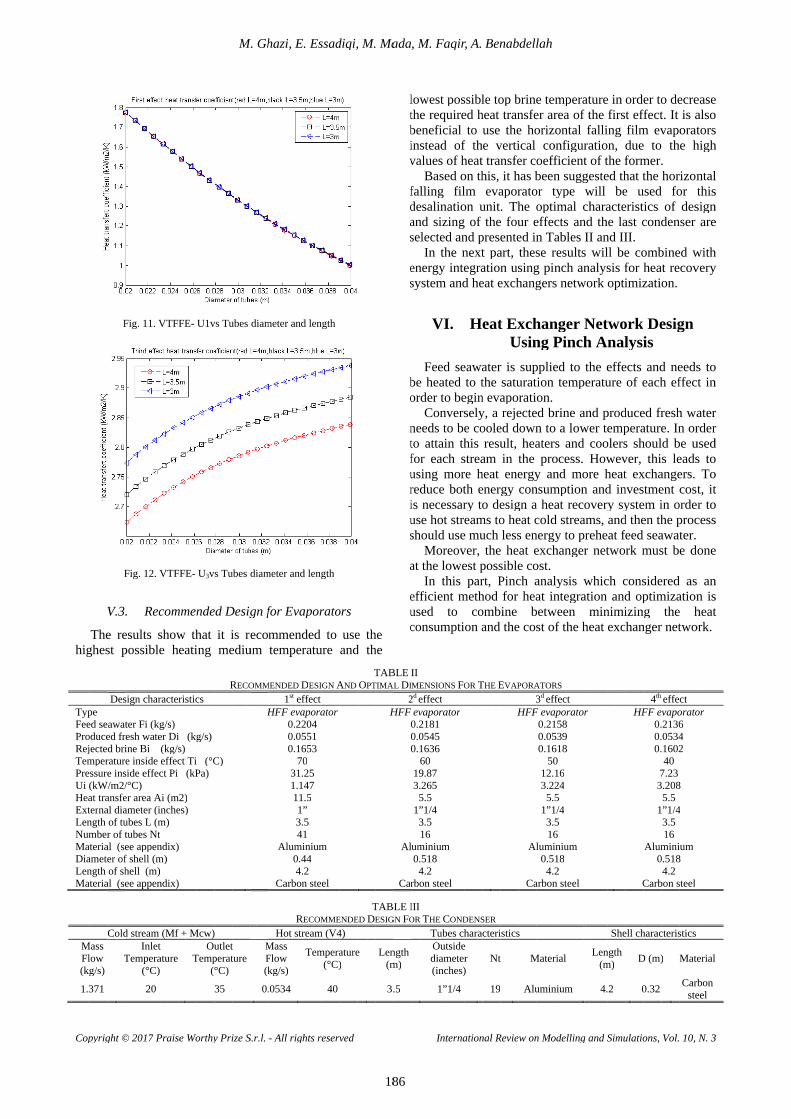
Copyright © 2017
highest possible heati
TypeFeed seawater Fi (kg/s)Produced fresh water Di (kg/s)Rejected brine Bi (kg/s)Temperature inside effect Ti (°C)Pressure inside effect Pi (kPa)Ui (kW/m2/°C)Heat transfer area Ai (m2)ExterLength of tubes L (m)Number of tubes NtMaterial (see appendix)Diameter of shell (m)Length of shell (m)Material (see appendix)
Mass Flow (kg/s)
1.371
Copyright © 2017
V.3.
The results show that it is recommended to use the highest possible heati
Type Feed seawater Fi (kg/s)Produced fresh water Di (kg/s)Rejected brine Bi (kg/s)Temperature inside effect Ti (°C)Pressure inside effect Pi (kPa)Ui (kW/m2/°C)Heat transfer area Ai (m2)External diameter (inches)Length of tubes L (m)Number of tubes NtMaterial (see appendix)Diameter of shell (m)Length of shell (m)Material (see appendix)
Mass Flow (kg/s)
1.371
Copyright © 2017
Fig.
Fig.
V.3.
The results show that it is recommended to use the highest possible heati
Design characteristics
Feed seawater Fi (kg/s)Produced fresh water Di (kg/s)Rejected brine Bi (kg/s)Temperature inside effect Ti (°C)Pressure inside effect Pi (kPa)Ui (kW/m2/°C)Heat transfer area Ai (m2)
nal diameter (inches)Length of tubes L (m)Number of tubes NtMaterial (see appendix)Diameter of shell (m)Length of shell (m)Material (see appendix)
Cold stream (Mf + Mcw)
Temperature
Copyright © 2017
Fig. 11.
Fig.
V.3.
The results show that it is recommended to use the highest possible heati
Design characteristics
Feed seawater Fi (kg/s)Produced fresh water Di (kg/s)Rejected brine Bi (kg/s)Temperature inside effect Ti (°C)Pressure inside effect Pi (kPa)Ui (kW/m2/°C) Heat transfer area Ai (m2)
nal diameter (inches)Length of tubes L (m)Number of tubes NtMaterial (see appendix)Diameter of shell (m)Length of shell (m)Material (see appendix)
Cold stream (Mf + Mcw)Inlet
Temperature (°
Copyright © 2017 Praise Worthy Prize S
11. VTFFE
12. VTFFE
Recommended Design for Evaporators
The results show that it is recommended to use the highest possible heati
Design characteristics
Feed seawater Fi (kg/s)Produced fresh water Di (kg/s)Rejected brine Bi (kg/s)Temperature inside effect Ti (°C)Pressure inside effect Pi (kPa)
Heat transfer area Ai (m2)
nal diameter (inches)Length of tubes L (m)Number of tubes Nt Material (see appendix)Diameter of shell (m)Length of shell (m) Material (see appendix)
Cold stream (Mf + Mcw)Inlet
Temperature (°C)
20
Praise Worthy Prize S
VTFFE
VTFFE
Recommended Design for Evaporators
The results show that it is recommended to use the highest possible heati
Design characteristics
Feed seawater Fi (kg/s) Produced fresh water Di (kg/s)Rejected brine Bi (kg/s)Temperature inside effect Ti (°C)Pressure inside effect Pi (kPa)
Heat transfer area Ai (m2)nal diameter (inches)
Length of tubes L (m)
Material (see appendix)Diameter of shell (m)
Material (see appendix)
Cold stream (Mf + Mcw)Inlet
Temperature
Praise Worthy Prize S
VTFFE-
VTFFE-
Recommended Design for Evaporators
The results show that it is recommended to use the highest possible heati
Design characteristics
Produced fresh water Di (kg/s)Rejected brine Bi (kg/s) Temperature inside effect Ti (°C)Pressure inside effect Pi (kPa)
Heat transfer area Ai (m2) nal diameter (inches)
Material (see appendix)
Material (see appendix)
Cold stream (Mf + Mcw)
Temperature Temperature
Praise Worthy Prize S
U1vs Tubes diameter and length
U3vs Tubes diameter and length
Recommended Design for Evaporators
The results show that it is recommended to use the highest possible heating medium temperature and the
Design characteristics
Produced fresh water Di (kg/s)
Temperature inside effect Ti (°C)Pressure inside effect Pi (kPa)
Cold stream (Mf + Mcw)Outlet
Temperature (°C)
35
Praise Worthy Prize S
U1vs Tubes diameter and length
vs Tubes diameter and length
Recommended Design for Evaporators
The results show that it is recommended to use the ng medium temperature and the
R
Temperature inside effect Ti (°C)
Cold stream (Mf + Mcw) Outlet
Temperature (°C)
35
M. Ghazi, E. Essadiqi, M. Mada, M. Faqir, A. Benabdellah
Praise Worthy Prize S
U1vs Tubes diameter and length
vs Tubes diameter and length
Recommended Design for Evaporators
The results show that it is recommended to use the ng medium temperature and the
RECOMMENDED
Outlet Temperature
M. Ghazi, E. Essadiqi, M. Mada, M. Faqir, A. Benabdellah
Praise Worthy Prize S.r.l.
U1vs Tubes diameter and length
vs Tubes diameter and length
Recommended Design for Evaporators
The results show that it is recommended to use the ng medium temperature and the
ECOMMENDED
HFF evaporator
Mass Flow (kg/s)
0.0534
M. Ghazi, E. Essadiqi, M. Mada, M. Faqir, A. Benabdellah
.r.l. - All rights reserved
U1vs Tubes diameter and length
vs Tubes diameter and length
Recommended Design for Evaporators
The results show that it is recommended to use the ng medium temperature and the
ECOMMENDED 1
HFF evaporator
Aluminium
Carbon steel
Hot stream (V4)Mass Flow (kg/s)
0.0534
M. Ghazi, E. Essadiqi, M. Mada, M. Faqir, A. Benabdellah
All rights reserved
U1vs Tubes diameter and length
vs Tubes diameter and length
Recommended Design for Evaporators
The results show that it is recommended to use the ng medium temperature and the
ECOMMENDED D1st effect
HFF evaporator0.22040.05510.1653
7031.251.14711.51”3.541
Aluminium0.444.2
Carbon steel
RECOMMENDED
Hot stream (V4)Mass Flow (kg/s)
0.0534
M. Ghazi, E. Essadiqi, M. Mada, M. Faqir, A. Benabdellah
All rights reserved
U1vs Tubes diameter and length
vs Tubes diameter and length
Recommended Design for Evaporators
The results show that it is recommended to use the ng medium temperature and the
DESIGN effect
HFF evaporator0.2204 0.0551 0.1653
70 31.25 1.147 11.5 1” 3.5 41
Aluminium0.44 4.2
Carbon steel
ECOMMENDED
Hot stream (V4)
Temperature
M. Ghazi, E. Essadiqi, M. Mada, M. Faqir, A. Benabdellah
All rights reserved
U1vs Tubes diameter and length
vs Tubes diameter and length
Recommended Design for Evaporators
The results show that it is recommended to use the ng medium temperature and the
ESIGN A
HFF evaporator
Aluminium
Carbon steel
ECOMMENDED
Hot stream (V4)
Temperature (°C)
40
M. Ghazi, E. Essadiqi, M. Mada, M. Faqir, A. Benabdellah
All rights reserved
Recommended Design for Evaporators
The results show that it is recommended to use the ng medium temperature and the
AND
ECOMMENDED
Hot stream (V4)
Temperature (°C)
M. Ghazi, E. Essadiqi, M. Mada, M. Faqir, A. Benabdellah
The results show that it is recommended to use the ng medium temperature and the
TABLE IIND OPTIMAL
TABLE IIIECOMMENDED DESIGN
Temperature
M. Ghazi, E. Essadiqi, M. Mada, M. Faqir, A. Benabdellah
186
The results show that it is recommended to use the ng medium temperature and the
TABLE IIPTIMAL
HFF evaporator
TABLE IIIESIGN
Length (m)
3.5
M. Ghazi, E. Essadiqi, M. Mada, M. Faqir, A. Benabdellah
186
lowest possible top brine temperature in order to decrease the required heat transfer area of the first effect. It is also beneficial to use the horizontal falling film evaporators instead of the vertical configuration, due tovalues of heat transfer coefficient of the former.
falling film evaporator type will be used for this desalination unit. The optimal characteristics of design and sizing of the four effectsselected and presente
energy integration using pinch analysis for heat recovery system and heat exchangers network optimization.
be heated to the saturation temperature of each effect in order to begin evaporation.
needs to beto attain this result, heaters and coolers should be used for each stream in the process. However, this leads to using more heat energy and more heat exchangers. To reduce both energy consumption and investment cost, it is necessause hot streams to heat cold streams, and then the process should use much less energy to preheat feed seawater.
at the lowest possible cost.
efficient method for heat integration and optimization is used to combine between minimizing the heat consumption and the cost of the heat exchanger network.
TABLE II
PTIMAL DIMENSIONS 2
HFF evaporator0.21810.05450.1636
Aluminium
Carbon steel
TABLE IIIESIGN FOR
Length (m)
3.5
M. Ghazi, E. Essadiqi, M. Mada, M. Faqir, A. Benabdellah
lowest possible top brine temperature in order to decrease the required heat transfer area of the first effect. It is also beneficial to use the horizontal falling film evaporators instead of the vertical configuration, due tovalues of heat transfer coefficient of the former.
Based on this, it has been suggested that the horizontal falling film evaporator type will be used for this desalination unit. The optimal characteristics of design and sizing of the four effectsselected and presente
In the next part, these results will be combined with energy integration using pinch analysis for heat recovery system and heat exchangers network optimization.
Feed seawater is supplied to the effects and needs to be heated to the saturation temperature of each effect in order to begin evaporation.
Conversely, a rejected brine and produced fresh water needs to beto attain this result, heaters and coolers should be used for each stream in the process. However, this leads to using more heat energy and more heat exchangers. To reduce both energy consumption and investment cost, it is necessause hot streams to heat cold streams, and then the process should use much less energy to preheat feed seawater.
Moreover, the heat exchanger network must be done at the lowest possible cost.
In this part, Piefficient method for heat integration and optimization is used to combine between minimizing the heat consumption and the cost of the heat exchanger network.
TABLE II IMENSIONS 2d effect
HFF evaporator0.21810.05450.1636
6019.873.2655.5
1”1/43.516
Aluminium0.5184.2
Carbon steel
TABLE III OR T
Length
M. Ghazi, E. Essadiqi, M. Mada, M. Faqir, A. Benabdellah
International Review on Modelli
lowest possible top brine temperature in order to decrease the required heat transfer area of the first effect. It is also beneficial to use the horizontal falling film evaporators instead of the vertical configuration, due tovalues of heat transfer coefficient of the former.
Based on this, it has been suggested that the horizontal falling film evaporator type will be used for this desalination unit. The optimal characteristics of design and sizing of the four effectsselected and presente
In the next part, these results will be combined with energy integration using pinch analysis for heat recovery system and heat exchangers network optimization.
VI.
Feed seawater is supplied to the effects and needs to be heated to the saturation temperature of each effect in order to begin evaporation.
Conversely, a rejected brine and produced fresh water needs to beto attain this result, heaters and coolers should be used for each stream in the process. However, this leads to using more heat energy and more heat exchangers. To reduce both energy consumption and investment cost, it is necessause hot streams to heat cold streams, and then the process should use much less energy to preheat feed seawater.
Moreover, the heat exchanger network must be done at the lowest possible cost.
In this part, Piefficient method for heat integration and optimization is used to combine between minimizing the heat consumption and the cost of the heat exchanger network.
IMENSIONS effect
HFF evaporator0.2181 0.0545 0.1636
60 19.87 3.265
5.5 1”1/4 3.5 16
Aluminium0.518
4.2 Carbon steel
THE CTubes characteristicsOutside diameter (inches)
1”1/4
M. Ghazi, E. Essadiqi, M. Mada, M. Faqir, A. Benabdellah
International Review on Modelli
lowest possible top brine temperature in order to decrease the required heat transfer area of the first effect. It is also beneficial to use the horizontal falling film evaporators instead of the vertical configuration, due tovalues of heat transfer coefficient of the former.
Based on this, it has been suggested that the horizontal falling film evaporator type will be used for this desalination unit. The optimal characteristics of design and sizing of the four effectsselected and presente
In the next part, these results will be combined with energy integration using pinch analysis for heat recovery system and heat exchangers network optimization.
VI.
Feed seawater is supplied to the effects and needs to be heated to the saturation temperature of each effect in order to begin evaporation.
Conversely, a rejected brine and produced fresh water needs to beto attain this result, heaters and coolers should be used for each stream in the process. However, this leads to using more heat energy and more heat exchangers. To reduce both energy consumption and investment cost, it is necessary to design a heat recovery system in order to use hot streams to heat cold streams, and then the process should use much less energy to preheat feed seawater.
Moreover, the heat exchanger network must be done at the lowest possible cost.
In this part, Piefficient method for heat integration and optimization is used to combine between minimizing the heat consumption and the cost of the heat exchanger network.
IMENSIONS FOR
HFF evaporator
Aluminium
Carbon steel
CONDENSER
Tubes characteristicsOutside diameter (inches)
1”1/4
M. Ghazi, E. Essadiqi, M. Mada, M. Faqir, A. Benabdellah
International Review on Modelli
lowest possible top brine temperature in order to decrease the required heat transfer area of the first effect. It is also beneficial to use the horizontal falling film evaporators instead of the vertical configuration, due tovalues of heat transfer coefficient of the former.
Based on this, it has been suggested that the horizontal falling film evaporator type will be used for this desalination unit. The optimal characteristics of design and sizing of the four effectsselected and presente
In the next part, these results will be combined with energy integration using pinch analysis for heat recovery system and heat exchangers network optimization.
Heat Exchanger Network
Feed seawater is supplied to the effects and needs to be heated to the saturation temperature of each effect in order to begin evaporation.
Conversely, a rejected brine and produced fresh water needs to be cooled down to a loto attain this result, heaters and coolers should be used for each stream in the process. However, this leads to using more heat energy and more heat exchangers. To reduce both energy consumption and investment cost, it
ry to design a heat recovery system in order to use hot streams to heat cold streams, and then the process should use much less energy to preheat feed seawater.
Moreover, the heat exchanger network must be done at the lowest possible cost.
In this part, Piefficient method for heat integration and optimization is used to combine between minimizing the heat consumption and the cost of the heat exchanger network.
OR T
ONDENSER
Tubes characteristicsOutside diameter (inches)
M. Ghazi, E. Essadiqi, M. Mada, M. Faqir, A. Benabdellah
International Review on Modelli
lowest possible top brine temperature in order to decrease the required heat transfer area of the first effect. It is also beneficial to use the horizontal falling film evaporators instead of the vertical configuration, due tovalues of heat transfer coefficient of the former.
Based on this, it has been suggested that the horizontal falling film evaporator type will be used for this desalination unit. The optimal characteristics of design and sizing of the four effectsselected and presente
In the next part, these results will be combined with energy integration using pinch analysis for heat recovery system and heat exchangers network optimization.
Heat Exchanger Network
Feed seawater is supplied to the effects and needs to be heated to the saturation temperature of each effect in order to begin evaporation.
Conversely, a rejected brine and produced fresh water cooled down to a lo
to attain this result, heaters and coolers should be used for each stream in the process. However, this leads to using more heat energy and more heat exchangers. To reduce both energy consumption and investment cost, it
ry to design a heat recovery system in order to use hot streams to heat cold streams, and then the process should use much less energy to preheat feed seawater.
Moreover, the heat exchanger network must be done at the lowest possible cost.
In this part, Piefficient method for heat integration and optimization is used to combine between minimizing the heat consumption and the cost of the heat exchanger network.
THE E
ONDENSER Tubes characteristics
Nt
19
M. Ghazi, E. Essadiqi, M. Mada, M. Faqir, A. Benabdellah
International Review on Modelli
lowest possible top brine temperature in order to decrease the required heat transfer area of the first effect. It is also beneficial to use the horizontal falling film evaporators instead of the vertical configuration, due tovalues of heat transfer coefficient of the former.
Based on this, it has been suggested that the horizontal falling film evaporator type will be used for this desalination unit. The optimal characteristics of design and sizing of the four effectsselected and presente
In the next part, these results will be combined with energy integration using pinch analysis for heat recovery system and heat exchangers network optimization.
Heat Exchanger NetworkUsing Pinch Analysis
Feed seawater is supplied to the effects and needs to be heated to the saturation temperature of each effect in order to begin evaporation.
Conversely, a rejected brine and produced fresh water cooled down to a lo
to attain this result, heaters and coolers should be used for each stream in the process. However, this leads to using more heat energy and more heat exchangers. To reduce both energy consumption and investment cost, it
ry to design a heat recovery system in order to use hot streams to heat cold streams, and then the process should use much less energy to preheat feed seawater.
Moreover, the heat exchanger network must be done at the lowest possible cost.
In this part, Pinch analysis which considered as an efficient method for heat integration and optimization is used to combine between minimizing the heat consumption and the cost of the heat exchanger network.
EVAPORATORS
HFF evaporator
Tubes characteristics
Nt
19
M. Ghazi, E. Essadiqi, M. Mada, M. Faqir, A. Benabdellah
International Review on Modelli
lowest possible top brine temperature in order to decrease the required heat transfer area of the first effect. It is also beneficial to use the horizontal falling film evaporators instead of the vertical configuration, due tovalues of heat transfer coefficient of the former.
Based on this, it has been suggested that the horizontal falling film evaporator type will be used for this desalination unit. The optimal characteristics of design and sizing of the four effectsselected and presented in T
In the next part, these results will be combined with energy integration using pinch analysis for heat recovery system and heat exchangers network optimization.
Heat Exchanger NetworkUsing Pinch Analysis
Feed seawater is supplied to the effects and needs to be heated to the saturation temperature of each effect in order to begin evaporation.
Conversely, a rejected brine and produced fresh water cooled down to a lo
to attain this result, heaters and coolers should be used for each stream in the process. However, this leads to using more heat energy and more heat exchangers. To reduce both energy consumption and investment cost, it
ry to design a heat recovery system in order to use hot streams to heat cold streams, and then the process should use much less energy to preheat feed seawater.
Moreover, the heat exchanger network must be done at the lowest possible cost.
nch analysis which considered as an efficient method for heat integration and optimization is used to combine between minimizing the heat consumption and the cost of the heat exchanger network.
VAPORATORS3
HFF evaporator
Aluminium
Carbon steel
Tubes characteristics
Material
Aluminium
M. Ghazi, E. Essadiqi, M. Mada, M. Faqir, A. Benabdellah
International Review on Modelli
lowest possible top brine temperature in order to decrease the required heat transfer area of the first effect. It is also beneficial to use the horizontal falling film evaporators instead of the vertical configuration, due tovalues of heat transfer coefficient of the former.
Based on this, it has been suggested that the horizontal falling film evaporator type will be used for this desalination unit. The optimal characteristics of design and sizing of the four effects
d in Tables II and III.In the next part, these results will be combined with
energy integration using pinch analysis for heat recovery system and heat exchangers network optimization.
Heat Exchanger NetworkUsing Pinch Analysis
Feed seawater is supplied to the effects and needs to be heated to the saturation temperature of each effect in order to begin evaporation.
Conversely, a rejected brine and produced fresh water cooled down to a lo
to attain this result, heaters and coolers should be used for each stream in the process. However, this leads to using more heat energy and more heat exchangers. To reduce both energy consumption and investment cost, it
ry to design a heat recovery system in order to use hot streams to heat cold streams, and then the process should use much less energy to preheat feed seawater.
Moreover, the heat exchanger network must be done at the lowest possible cost.
nch analysis which considered as an efficient method for heat integration and optimization is used to combine between minimizing the heat consumption and the cost of the heat exchanger network.
VAPORATORS3d effect
HFF evaporator0.21580.05390.1618
5012.163.2245.5
1”1/43.516
Aluminium0.5184.2
Carbon steel
Material
Aluminium
International Review on Modelli
lowest possible top brine temperature in order to decrease the required heat transfer area of the first effect. It is also beneficial to use the horizontal falling film evaporators instead of the vertical configuration, due tovalues of heat transfer coefficient of the former.
Based on this, it has been suggested that the horizontal falling film evaporator type will be used for this desalination unit. The optimal characteristics of design and sizing of the four effects
ables II and III.In the next part, these results will be combined with
energy integration using pinch analysis for heat recovery system and heat exchangers network optimization.
Heat Exchanger NetworkUsing Pinch Analysis
Feed seawater is supplied to the effects and needs to be heated to the saturation temperature of each effect in order to begin evaporation.
Conversely, a rejected brine and produced fresh water cooled down to a lo
to attain this result, heaters and coolers should be used for each stream in the process. However, this leads to using more heat energy and more heat exchangers. To reduce both energy consumption and investment cost, it
ry to design a heat recovery system in order to use hot streams to heat cold streams, and then the process should use much less energy to preheat feed seawater.
Moreover, the heat exchanger network must be done
nch analysis which considered as an efficient method for heat integration and optimization is used to combine between minimizing the heat consumption and the cost of the heat exchanger network.
VAPORATORS effect
HFF evaporator0.2158 0.0539 0.1618
50 12.16 3.224 5.5
1”1/4 3.5 16
Aluminium0.518 4.2
Carbon steel
Material
Aluminium
International Review on Modelling and Simulations, Vol. 10, N. 3
lowest possible top brine temperature in order to decrease the required heat transfer area of the first effect. It is also beneficial to use the horizontal falling film evaporators instead of the vertical configuration, due tovalues of heat transfer coefficient of the former.
Based on this, it has been suggested that the horizontal falling film evaporator type will be used for this desalination unit. The optimal characteristics of design
and the last condenser are ables II and III.
In the next part, these results will be combined with energy integration using pinch analysis for heat recovery system and heat exchangers network optimization.
Heat Exchanger NetworkUsing Pinch Analysis
Feed seawater is supplied to the effects and needs to be heated to the saturation temperature of each effect in
Conversely, a rejected brine and produced fresh water cooled down to a lower temperature. In order
to attain this result, heaters and coolers should be used for each stream in the process. However, this leads to using more heat energy and more heat exchangers. To reduce both energy consumption and investment cost, it
ry to design a heat recovery system in order to use hot streams to heat cold streams, and then the process should use much less energy to preheat feed seawater.
Moreover, the heat exchanger network must be done
nch analysis which considered as an efficient method for heat integration and optimization is used to combine between minimizing the heat consumption and the cost of the heat exchanger network.
HFF evaporator
Aluminium
Carbon steel
Aluminium
ng and Simulations, Vol. 10, N. 3
lowest possible top brine temperature in order to decrease the required heat transfer area of the first effect. It is also beneficial to use the horizontal falling film evaporators instead of the vertical configuration, due tovalues of heat transfer coefficient of the former.
Based on this, it has been suggested that the horizontal falling film evaporator type will be used for this desalination unit. The optimal characteristics of design
and the last condenser are ables II and III.
In the next part, these results will be combined with energy integration using pinch analysis for heat recovery system and heat exchangers network optimization.
Heat Exchanger NetworkUsing Pinch Analysis
Feed seawater is supplied to the effects and needs to be heated to the saturation temperature of each effect in
Conversely, a rejected brine and produced fresh water wer temperature. In order
to attain this result, heaters and coolers should be used for each stream in the process. However, this leads to using more heat energy and more heat exchangers. To reduce both energy consumption and investment cost, it
ry to design a heat recovery system in order to use hot streams to heat cold streams, and then the process should use much less energy to preheat feed seawater.
Moreover, the heat exchanger network must be done
nch analysis which considered as an efficient method for heat integration and optimization is used to combine between minimizing the heat consumption and the cost of the heat exchanger network.
Length (m)
4.2
ng and Simulations, Vol. 10, N. 3
lowest possible top brine temperature in order to decrease the required heat transfer area of the first effect. It is also beneficial to use the horizontal falling film evaporators instead of the vertical configuration, due tovalues of heat transfer coefficient of the former.
Based on this, it has been suggested that the horizontal falling film evaporator type will be used for this desalination unit. The optimal characteristics of design
and the last condenser are ables II and III.
In the next part, these results will be combined with energy integration using pinch analysis for heat recovery system and heat exchangers network optimization.
Heat Exchanger NetworkUsing Pinch Analysis
Feed seawater is supplied to the effects and needs to be heated to the saturation temperature of each effect in
Conversely, a rejected brine and produced fresh water wer temperature. In order
to attain this result, heaters and coolers should be used for each stream in the process. However, this leads to using more heat energy and more heat exchangers. To reduce both energy consumption and investment cost, it
ry to design a heat recovery system in order to use hot streams to heat cold streams, and then the process should use much less energy to preheat feed seawater.
Moreover, the heat exchanger network must be done
nch analysis which considered as an efficient method for heat integration and optimization is used to combine between minimizing the heat consumption and the cost of the heat exchanger network.
Shell
Length (m)
4.2
ng and Simulations, Vol. 10, N. 3
lowest possible top brine temperature in order to decrease the required heat transfer area of the first effect. It is also beneficial to use the horizontal falling film evaporators instead of the vertical configuration, due tovalues of heat transfer coefficient of the former.
Based on this, it has been suggested that the horizontal falling film evaporator type will be used for this desalination unit. The optimal characteristics of design
and the last condenser are ables II and III.
In the next part, these results will be combined with energy integration using pinch analysis for heat recovery system and heat exchangers network optimization.
Heat Exchanger Network Using Pinch Analysis
Feed seawater is supplied to the effects and needs to be heated to the saturation temperature of each effect in
Conversely, a rejected brine and produced fresh water wer temperature. In order
to attain this result, heaters and coolers should be used for each stream in the process. However, this leads to using more heat energy and more heat exchangers. To reduce both energy consumption and investment cost, it
ry to design a heat recovery system in order to use hot streams to heat cold streams, and then the process should use much less energy to preheat feed seawater.
Moreover, the heat exchanger network must be done
nch analysis which considered as an efficient method for heat integration and optimization is used to combine between minimizing the heat consumption and the cost of the heat exchanger network.
HFF evaporator
Carbon steel
Shell characteristics
D (m)
0.32
ng and Simulations, Vol. 10, N. 3
lowest possible top brine temperature in order to decrease the required heat transfer area of the first effect. It is also beneficial to use the horizontal falling film evaporators instead of the vertical configuration, due tovalues of heat transfer coefficient of the former.
Based on this, it has been suggested that the horizontal falling film evaporator type will be used for this desalination unit. The optimal characteristics of design
and the last condenser are
In the next part, these results will be combined with energy integration using pinch analysis for heat recovery system and heat exchangers network optimization.
Heat Exchanger Network Design Using Pinch Analysis
Feed seawater is supplied to the effects and needs to be heated to the saturation temperature of each effect in
Conversely, a rejected brine and produced fresh water wer temperature. In order
to attain this result, heaters and coolers should be used for each stream in the process. However, this leads to using more heat energy and more heat exchangers. To reduce both energy consumption and investment cost, it
ry to design a heat recovery system in order to use hot streams to heat cold streams, and then the process should use much less energy to preheat feed seawater.
Moreover, the heat exchanger network must be done
nch analysis which considered as an efficient method for heat integration and optimization is used to combine between minimizing the heat consumption and the cost of the heat exchanger network.
4th
HFF evaporator0.21360.0530.1602
7.233.208
1”1/4
Aluminium0.518
Carbon steel
characteristics
D (m)
0.32
ng and Simulations, Vol. 10, N. 3
lowest possible top brine temperature in order to decrease the required heat transfer area of the first effect. It is also beneficial to use the horizontal falling film evaporators instead of the vertical configuration, due to the high values of heat transfer coefficient of the former.
Based on this, it has been suggested that the horizontal falling film evaporator type will be used for this desalination unit. The optimal characteristics of design
and the last condenser are
In the next part, these results will be combined with energy integration using pinch analysis for heat recovery system and heat exchangers network optimization.
Design
Feed seawater is supplied to the effects and needs to be heated to the saturation temperature of each effect in
Conversely, a rejected brine and produced fresh water wer temperature. In order
to attain this result, heaters and coolers should be used for each stream in the process. However, this leads to using more heat energy and more heat exchangers. To reduce both energy consumption and investment cost, it
ry to design a heat recovery system in order to use hot streams to heat cold streams, and then the process should use much less energy to preheat feed seawater.
Moreover, the heat exchanger network must be done
nch analysis which considered as an efficient method for heat integration and optimization is used to combine between minimizing the heat consumption and the cost of the heat exchanger network.
th effectHFF evaporator
0.21360.05340.1602
40 7.23
3.2085.5
1”1/43.5 16
Aluminium0.518
4.2 Carbon steel
characteristics
D (m)
ng and Simulations, Vol. 10, N. 3
lowest possible top brine temperature in order to decrease the required heat transfer area of the first effect. It is also beneficial to use the horizontal falling film evaporators
the high
Based on this, it has been suggested that the horizontal falling film evaporator type will be used for this desalination unit. The optimal characteristics of design
and the last condenser are
In the next part, these results will be combined with energy integration using pinch analysis for heat recovery
Design
Feed seawater is supplied to the effects and needs to be heated to the saturation temperature of each effect in
Conversely, a rejected brine and produced fresh water wer temperature. In order
to attain this result, heaters and coolers should be used for each stream in the process. However, this leads to using more heat energy and more heat exchangers. To reduce both energy consumption and investment cost, it
ry to design a heat recovery system in order to use hot streams to heat cold streams, and then the process should use much less energy to preheat feed seawater.
Moreover, the heat exchanger network must be done
nch analysis which considered as an efficient method for heat integration and optimization is used to combine between minimizing the heat consumption and the cost of the heat exchanger network.
effect HFF evaporator
0.2136 4
0.1602
3.208
1”1/4
Aluminium 0.518
Carbon steel
characteristics
Material
Carbon steel
ng and Simulations, Vol. 10, N. 3
lowest possible top brine temperature in order to decrease the required heat transfer area of the first effect. It is also beneficial to use the horizontal falling film evaporators
the high
Based on this, it has been suggested that the horizontal falling film evaporator type will be used for this desalination unit. The optimal characteristics of design
and the last condenser are
In the next part, these results will be combined with energy integration using pinch analysis for heat recovery
Design
Feed seawater is supplied to the effects and needs to be heated to the saturation temperature of each effect in
Conversely, a rejected brine and produced fresh water wer temperature. In order
to attain this result, heaters and coolers should be used for each stream in the process. However, this leads to using more heat energy and more heat exchangers. To reduce both energy consumption and investment cost, it
ry to design a heat recovery system in order to use hot streams to heat cold streams, and then the process
Moreover, the heat exchanger network must be done
nch analysis which considered as an efficient method for heat integration and optimization is used to combine between minimizing the heat consumption and the cost of the heat exchanger network.
HFF evaporator
Material
Carbon steel
ng and Simulations, Vol. 10, N. 3
lowest possible top brine temperature in order to decrease the required heat transfer area of the first effect. It is also beneficial to use the horizontal falling film evaporators
the high
Based on this, it has been suggested that the horizontal falling film evaporator type will be used for this desalination unit. The optimal characteristics of design
and the last condenser are
In the next part, these results will be combined with energy integration using pinch analysis for heat recovery
Feed seawater is supplied to the effects and needs to be heated to the saturation temperature of each effect in
Conversely, a rejected brine and produced fresh water wer temperature. In order
to attain this result, heaters and coolers should be used for each stream in the process. However, this leads to using more heat energy and more heat exchangers. To reduce both energy consumption and investment cost, it
ry to design a heat recovery system in order to use hot streams to heat cold streams, and then the process
Moreover, the heat exchanger network must be done
nch analysis which considered as an efficient method for heat integration and optimization is used to combine between minimizing the heat consumption and the cost of the heat exchanger network.
Material
Carbon

M. Ghazi, E. Essadiqi, M. Mada, M. Faqir, A. Benabdellah
Copyright © 2017 Praise Worthy Prize S.r.l. - All rights reserved International Review on Modelling and Simulations, Vol. 10, N. 3
187
In other words, the objective is to minimize the total cost. In this section, pinch analysis and its methodology is used to identify the optimal heat exchanger network for the present seawater desalination unit, the methodology is in four steps.
First step is extracting stream data from process flow-sheet. Second step is selecting the minimum temperature difference values ∆Tmin. Third step is sizing and designing the heat exchangers and finally the fourth step is the selection of the optimal design which allows the minimum total cost.
VI.1. Stream Data Extraction for three Possible Configurations
Mixing can cause problems in stream data extraction. Process streams of the same composition leaving each effect at different temperatures could be mixed and considered as one stream, and then, the heating could be performed by single heat exchanger. However, mixing will degrade temperatures and reduce the driving forces
in heat exchangers, giving increased capital cost. Indeed, the partial flows of reject brine, produced distilled water, and feed seawater could be mixed in a different manner which gives three possible configurations of streams as shown in Figs. 13 and Tables IV, V and VI.
VI.2. The Minimum Temperature Difference ∆Tmin
Lower values of ∆Tmin give lower hot and cold utilities but larger and more costly heat exchangers; this is so because the heat transfer area needed is inversely proportional to the temperature difference. So, small values of ∆Tmin can lead to very large heat exchangers. The cost of thermal heat required for feed sweater heating is proportional to energy usage which decreases when ∆Tmin becomes smaller. If we sum the operating and capital cost, the total cost (annualized heat cost and capital costs) passes through a minimum value which corresponds to the optimal ∆Tmin [30]. In this study we have considered five values of which are: 2, 4, 6, 8, and 10°C.
(1) (3)
(2)
Figs. 13. Three possible configurations for streams mixing (configurations 1, 2 and 3)

M. Ghazi, E. Essadiqi, M. Mada, M. Faqir, A. Benabdellah
Copyright © 2017 Praise Worthy Prize S.r.l. - All rights reserved International Review on Modelling and Simulations, Vol. 10, N. 3
188
TABLE IV STREAMS DATA FOR CONFIGURATION (1)
Stream Nature of stream
M (kg/s)
CP (kW/K)
Ti (°C)
Tf (°C)
Q (kW)
F1 Cold Stream 0.2204 0,9212 35 70 32.24 F2 Cold Stream 0.2181 0,9116 35 60 22.79 F3 Cold Stream 0.2158 0,9020 35 50 13.53 F4 Cold Stream 0.2136 0,8928 35 40 4.46 B1 Hot stream 0.1587 0,6633 70 30 23.21 B2 Hot stream 0.1570 0,6562 60 30 16.40 B3 Hot stream 0.1554 0,6495 50 30 9.74 B4 Hot stream 0.1538 0,6428 40 30 3.21 D1 Hot stream 0.0617 0,2579 70 30 9.02 D2 Hot stream 0.0611 0,2553 60 30 6.38 D3 Hot stream 0.0604 0,2524 50 30 3.78 D4 Hot stream 0.0598 0,2499 40 30 1.25
TABLE V
STREAMS DATA FOR CONFIGURATION (3)
Stream Nature of stream
M (kg/s)
CP (kW/K) Ti (°C) Tf
(°C) Q (kW)
Mf1 Cold Stream 0.4384 1,8325 35 70 64.13 Mf2 Cold Stream 0.4294 1,7948 35 50 26.92 Md1 Hot stream 0.1228 0,5133 65 35 15.39 Md2 Hot stream 0.1202 0,5024 45 35 5.02 Mb1 Hot stream 0.3157 1,3196 65 35 39.59 Mb2 Hot stream 0.3092 1,2924 45 35 12.92
TABLE VI STREAMS DATA FOR CONFIGURATION (2)
Stream Nature of stream
M (kg/s)
CP (kW/K)
Ti (°C)
Tf (°C)
Q (kW)
Mf Cold stream 0.868 3,628 35 70 127 Md Hot stream 0.243 1,016 55 35 20.3 Mb Hot stream 0.625 2,612 55 35 52.2
VI.3. Heat Exchangers Selection and Sizing
It is of great importance to make appropriate choices when it comes to heat exchanger types and material to ensure proper operation to avoid, as much as possible, problems that may limit the heat exchanger and heat recovery efficiency.
The choice of the suitable type of heat exchanger depends on several parameters, essentially, cost, heat transfer coefficient, and maintenance. It was found out that the most suitable type of heat exchanger for our plant is the plate type heat exchanger; its characteristics are shown in Fig. 14 and Table VII.
Fig. 14. Plate dimensions–Plate heat exchanger
TABLE VII PLATE HEAT EXCHANGER CHARACTERISTICS
W (m) L (m) b(m) Area per plate (m2) 0,25 0,56 0,004 0,88
For the plate heat exchangers, heat transfer rate can be
evaluated based on the correlations of the most widely used plates for the turbulent flow [34]:
푁푢 = 0,374푅푒 , 푃푟 , (µ /µ ) , (39)
where the Reynolds number Re is based on equivalent diameter, De, defined by:
퐷 =4푊푏
2(푊 + 푏) (40)
For laminar flow:
푁푢 = 푐 (푅푒푃푟퐷퐿
) , (µ /µ ) , (41)
where c1= 1.86-4.50 depending on geometry, and L is the effective plate length.
VI.4. Case study: Configuration C & ∆Tmin=2°C
It is recalled that the pinch analysis is applied for three different configurations (1, 2, and 3) with five different values of ∆Tmin (2, 4, 6, 8 and 10°C), which means fifteen cases. Configuration 2 and a minimum temperature difference of 2°C are selected in this case study.
VI.4.1. Shifted Temperatures
The shifted temperatures are set at 1⁄2×∆Tmin above cold stream temperatures and 1⁄2×∆Tmin below hot stream temperatures. They are used to ensure that the temperature differences between hot streams and cold streams are equal to or greater than ΔTmin. Data for shifted temperatures for this case study are shown in Table VIII.
TABLE VIII TARGET AND SHIFTED TEMPERATURES
Stream data Target temperatures Shifted temperatures
Stream Nature of stream Ti (°C) Tf
(°C) T*i (°C) T*f (°C)
Mf Cold stream 35 70 36 71 Md Hot stream 55 35 54 34 Mb Hot stream 55 35 55 34
VI.4.2. Temperature Intervals
Figure 15 shows that streams’ data are divided into three temperature intervals (I, II, and III), each interval represents a sub-network. And each interval is defined by a process stream supply and target temperature. For each sub-network, there is either a net heat deficit or surplus, but never both. As a sign convention, a heat deficit is considered negative and a heat surplus is considered positive.

M. Ghazi, E. Essadiqi, M. Mada, M. Faqir, A. Benabdellah
Copyright © 2017 Praise Worthy Prize S.r.l. - All rights reserved International Review on Modelling and Simulations, Vol. 10, N. 3
189
Fig. 15. Temperatures intervals - configuration c, ∆Tmin=2°C
VI.4.3. Problem Table Cascade
In the problem table cascade the heat input from external utility is assumed equal to zero and the heat surplus from higher temperature interval can be used to make up for heat deficit of lower temperature intervals. For each sub-network the output is calculated by adding the surplus to the input, the calculation of heat in this manner is shown in Fig. 16.
In order to have a feasible configuration, the transmission of heat from high temperature interval to low temperature interval must be positive. Therefore, if negative values are obtained, the external hot utility must be increased from zero to a minimum positive value in order to make all heat flows positive or equal to zero. In addition to this, the minimum cold utility is equal to the heat flow out of the coldest sub-network.
Fig. 16. Problem table cascade - configuration c, ∆Tmin=2°C
VI.4.4. Grid Diagram
In the grid diagram representation, as shown in Fig. 17, hot streams (rejected brine and distillate) are represented at the top of their supply temperatures on the left side to target temperatures on the right side.
Cold stream (feed seawater)is represented below hot streams and it runs in countercurrent direction. Also, in the grid diagram, the heat exchanger network is constructed according to [30].
VI.5. Results and Discussion for Heat Exchanger Network Design Using Pinch Analysis
VI.5.1. Determination of the Optimal ∆Tmin
From the graphical representation of the annualized hot utility cost, the investment cost and the total cost
depending on the minimum temperature difference ∆Tmin for the three configurations 1, 2 and 3, it is known that the optimal value of ∆Tmin is approximately equal to 6°C as shown in Figs.18, 19 and 20.
VI.5.2. Optimal Design of the Heat Exchanger Network
It is obvious from Fig. 21 that the configuration 2 is the most advantageous compared to configuration 1 and 3; consequently, the configuration 2 was selected to be used for the final design of heat exchanger network. In this case the total cost passes through a minimum value of 14000 US Dollar which corresponds to ∆Tmin=6°C.
Fig. 17. Grid diagram - configuration c, ∆Tmin=2°C
Fig. 18. Variation of different costs vs ∆Tmin for configuration (1)
Fig. 19. Variation of different costs vs ∆Tmin for configuration (2)

M. Ghazi, E. Essadiqi, M. Mada, M. Faqir, A. Benabdellah
Copyright © 2017 Praise Worthy Prize S.r.l. - All rights reserved International Review on Modelling and Simulations, Vol. 10, N. 3
190
Fig. 20. Variation of different costs vs ∆Tmin for the configuration (3)
Fig. 21. Total cost for the three configurations
The final design of heat exchanger network includes four heat exchangers as shown in Fig. 22. The heat exchangers (1) and (2) are used for heat recovery from produced fresh water and rejected brine, respectively. Besides, the additional heat exchangers (a) and (b) are used in order to increase feed seawater in order to achieve the target temperature for both the first effect and the second one.
Fig. 22. Final design of heat exchanger network Under steady-state conditions and in the region of the
optimum (configuration 2 and ∆Tmin=6°C) the sensible heat recovery is approximately equal to 50.79 kW, and the sensible heat consumption used for feed seawater
heating is equal to 29.37 kW. The results of heat exchangers sizing are given in the Table IX.
The total heat consumption of this pilot unit is about 158 kW, the last condenser is used to condense the steam of the last effect (effect 4), and also it’s used to preheat feed seawater from 20°C to 35°C. The heat recovered using the condenser is about 54.42 kW. The feed seawater is heated from 35°C to 49°C using the heat recovery heat exchangers (1) and (2).
TABLE IX
NUMERICAL RESULTS OF HEAT EXCHANGERS SIZING
Heat exchanger Thermal power (kW)
Required total area (m2)
Number of plates
(a) 20,23 0,741 9 (b) 10,93 0,314 4 (1) 14,18 0,872 10 (2) 36,48 1,720 20
VII. Experimental Validation of Sizing Results
The developed model is used for the same design and operating conditions stated in literature in order to check its validity. Reference [32]presented the experimental measurements for small vertically-stacked MED plants of the horizontal tube falling film evaporators type using hot water as the thermal energy source for the first effect.
As shown in the Table X, using the same data stated by [32] the model results show good agreement with the experimental values. Indeed, the numerical results obtained in this model are compared to the experimental values for the overall heat transfer coefficient. The comparison shows that the values are highly similar and error doesn’t exceed 1 %. However, the error obtained for the condenser calculations is about 15 %.
In the case of using vertical tubes falling film evaporators, the model is validated based on the data and results stated in reference [33]. As shown in Table XI, results show that the error of calculating the overall heat transfer coefficients doesn’t exceed 15%.
TABLE X
COMPARISON BETWEEN LITERATURE RESULTS AND THE DEVELOPED MODEL FOR HTFF EVAPORATORS
Effect Feed (kg/s)
Ti-
1(°C) Ti (°C) U (W/°C/m2)
Error (%) Model Ref [30]
1 4,84 76- 67 63,1 1886,8 1885,2 0,09 2 4,75 63,1 61,75 3339,0
3343,6 0,14
3 4,67 61,75 60,34 3333,1 0,31 4 4,59 60,34 58,91 3328,6 0,45
Cond 10 31.79 39.45 1578,0 1870,1 15,62
TABLE XI COMPARISON BETWEEN LITERATURE RESULTS AND THE DEVELOPED
MODEL FOR VTFF EVAPORATORS
Case Feed (kg/s) Ti-1(°C) Ti
(°C) U (W/°C/m2) Error
(%) Model Ref [31] 1 0,667 95 81,4 2289,8 2461 7 2 0,667 95 68 2045,9 2129 4
3 0,334 95 77 2188 2582 15

M. Ghazi, E. Essadiqi, M. Mada, M. Faqir, A. Benabdellah
Copyright © 2017 Praise Worthy Prize S.r.l. - All rights reserved International Review on Modelling and Simulations, Vol. 10, N. 3
191
VIII. Conclusion In this paper, the optimal design and sizing of new
solar driven seawater desalination pilot unit is studied and presented. The unit uses a four effect evaporation process technology with a production capacity of 7m3/day of fresh water obtained from the evaporation of 28% of feed seawater. The developed model is validated based on published results in the literature; it is also flexible and could also be used for designing large production capacities.
This paper is composed of two complementary sections. The first one deals with the thermal analysis, modeling and the optimizing the evaporation process. The second one deals with the optimization of the heat exchangers network based on the Pinch analysis method. The obtained results show that using the horizontal tubes falling film evaporators is more advantageous compared to vertical tubes configuration in terms of the heat transfer rate, maintenance rate, and the ease of cleaning and use.
Indeed, the obtained heat transfer coefficients range between 3.18 and 3.32kW/m2/K when using horizontal falling film evaporators and between 2.15 and 2.4kW/m2/K for vertical falling film evaporators when using the optimal tubes’ dimensions. Moreover, this study reveals that the first effect heat transfer area could be reduced by increasing the heating medium temperature and decreasing the top brine temperature. The optimization of the evaporation unit is then completed by Pinch analysis method for three possible heat exchanger networks to be used for heat recovery and feed seawater heating. The most optimal configuration can reach a reduction of 62% of the thermal power needed for seawater heating.
The most relevant criteria and results obtained from this study are summarized as follow: Using horizontal falling evaporators is more
advantageous when compared to the other evaporators’ types;
The design of the first effect differs from the other effects because it uses hot water as a heating medium instead of using vapor;
Decreasing the first effect diameter increases the heat transfer rate, however the other effects show an opposite behavior towards the diameter change;
The selection of the optimal temperature difference and the suitable heat exchanger network configuration lead to a notable reduction of the required thermal power.
Acknowledgements
Financial support; of the “Moroccan Agency for Solar Energy IRESEN” for “Seawater desalination using solar energy” project; is cordially appreciated and gratefully acknowledged.
References [1] E.Delyannis, V.Belessiotis, Desalination: The recent development
path, Desalination 264 (2010) 206–213. [2] S. Al-Mutaz, Irfan Wazeer, Development of a steady-state
mathematical model for MEE-TVC desalination plants, Desalination 351 (2014) 9-18.
[3] Hisham El-Dessouky, ImadAlatiqi, S. Bingulac and Hisham Ettouney, Steady-State Analysis of the Multiple Effect Evaporation Desalination Process, Chem. Eng. Technol. 21 (1998) 437-451.
[4] Darwish M.A.; El-Dessouky, The heat recovery thermal vapour-compression desalting system: A comparison with other thermal desalination processes, Applied Thermal Engineering, Volume 16, Issue 6, June 1996, Pages 523-537.
[5] M.H. Khademi, M.R. Rahimpour, A. Jahanmiri, Simulation and optimization of a six-effect evaporator in a desalination process, Chemical Engineering and Processing 48 (2009) 339–347.
[6] Seyed Ehsan Shakib, Majid Amidpour , Cyrus Aghanajafi, Simulation and optimization of multi effect desalination coupled to a gas turbine plant with HRSG consideration, Desalination 285 (2012) 366–376.
[7] Hisham T. El-Dessoukya,, Hisham M. Ettouneya, Faisal Mandani, Performance of parallel feed multiple effect evaporation system for seawater desalination, Applied Thermal Engineering 20 (2000) 1679-1706.
[8] Patricia Palenzuela, Ashraf S. Hassan, Guillermo Zaragoza, Diego-C. Alarcón-Padilla, Steady state model for multi-effect distillation case study: Plataforma Solar de Almería MED pilot plant, Desalination 337 (2014) 31–42.
[9] Ibrahim S. Al-Mutaz, IrfanWazeer, Comparative performance evaluation of conventional multi-effect evaporation desalination processes, Applied Thermal Engineering 73 (2014) 1192-1201.
[10] İbrahim Halil Yılmaz , Mehmet Sait Söylemez, Design and computer simulation on multi-effect evaporation seawater desalination system using hybrid renewable energy sources in Turkey, Desalination 291 (2012) 23–40.
[11] Narmine H. Aly, Adel K. El-Fiqi, Thermal performance of seawater desalination systems, Desalination 158 (2003) 127-142.
[12] Ali M. El-Nashar, Amer A. Qamhiyeh, Simulation of the steady-state operation of a multi-effect stack seawater distillation plant, Desalination 101 (1995) 231-243.
[13] A.M. El-Nashar, M. Samad, The solar desalination plant in Abu Dhabi: 13 years of performance and operation history, Renewable Energy 14 (1998) 263–274.
[14] Ali M. El-Nashar and Amer A. Qamhiyeh, Performance Simulation of the Heat Accumulator of the Abu dhabi Solar Desalination Plant, Solar Energy Vol. 44. No 4,(1990) pp. 183-191.
[15] Ali M. El-Nashar, Performance of the Solar Desalination Plant at Abu Dhabi, Desalination, 72 (1989) 405-424.
[16] Ali M. El-Nashar and Amer A. Qamhiyeh, Simulation of the Performance of MES Evaporators Under Unsteady State Operating Conditions, Desalination, 79 (1990) 65-83.
[17] Khaled M.Bataineh, Multi-effect desalination plant combined with thermal compressor driven by steam generated by solar energy, Desalination 385 (2016) 39–52.
[18] German Solar Energy Society, Planning & Installing Solar Thermal Systems, second edition,(2010) pp 96-97.
[19] Bela M. Fabuss and Alexander korosi, Boiling point Elevations of Seawater and It Concentrates, Journal of Chemical and Engineering Data, Vol. 11, N°4, October 1966, pp 606-609.
[20] Vincent Y. Lister, John F. Davidson, D. Ian Wilson, Calculating thermal fouling resistances from dynamic heat transfer measurements, Chemical Engineering Science 84 (2012) 772–780.
[21] D.Q. Kern, R.E. Seaton, A theoretical analysis of thermal surface fouling, Chem. Eng. Prog. 4 (1959) 258–262.
[22] A. Paul Watkznson, Process Heat Transfer: Some Practical Problems, The Canadian Journal of Chemical Engineering, Vol. 58, October 1980, PP : 553-558.
[23] D.Q. Kern, Process Heat Transfer, International Student Edition, 1950.
[24] Paul E. Minton, Handbook of Evaporation Technology, Noyes

M. Ghazi, E. Essadiqi, M. Mada, M. Faqir, A. Benabdellah
Copyright © 2017 Praise Worthy Prize S.r.l. - All rights reserved International Review on Modelling and Simulations, Vol. 10, N. 3
192
publications, Westwood, Newjersy USA, 1986, pp 11-14. [25] H.T. El-Dessouky, H.M. Ettoney, Fundamentals of Salt Water
Desalination, first edition 2002, Annexes pp 586-598. [26] Chung &Seban (1971). Transactions of ASME, Journal of Heat
Transfer, Section C, 93, 391. [27] Xingsen Mu, Shengqiang Shen, Yong Yang &Xiaohua Liu (2012)
Experimental study of falling film evaporation heat transfer coefficient on horizontal tube, Desalination and Water Treatment, 50:1-3, 310-316. DOI: 10.1080/19443994.2012.719734
[28] Shengqiang Shen, Rui Liu , Yong Yang, Xiaohua Liu &Juexian Chen (2011) Condensation character of a stratified flow inside a horizontal tube, Desalination and Water Treatment, 33:1-3, 218-223.
[29] Shengqiang Shen, Luyuan Gong, Hua Liu, Xingsen Mu, Rui Liu, Characteristic study of steam maldistribution in horizontal-tube falling film evaporators, Applied Thermal Engineering 75(2015) 1-13.
[30] B. Linnhoff, E. Hindmarsh, The Pinch design method for heat exchanger networks, Chem. Eng. Sci. 38 (1983) 745-763.
[31] Desalting handbook for planners, Third Edition by RosTek Associates, Inc., Tampa, Florida Agreement Number: 98-PG-81-0366 Desalination Research and Development Program Report No. 72 July 2003.
[32] Ali M. El-Nashar, Predicting part load performance of small MED evaporators -a simple simulation program and its experimental verification, Desalination 130 (2000) 217-234.
[33] Sandro Angeletti and Mauro Mores, Modelling of multiple-effect falling-film evaporators, J. Fd Technol. (1983) 18,539-563.
[34] Manoj B. Kumbhare and S. D. Dawande, Performance evaluation of plate heat exchanger in laminar and turbulent flow conditions, International Journal of Chemical Sciences and Applications, Vol 4, Issue 1, 2013, pp 77-83.
[35] Yousefi, M., Yousefi, M., Khaksar, W., B. Ismail Alnaimi, F., Nordin Darus, A., A Comprehensive Review on the Application of Evolutionary Computation in Design Optimization of Plate-Fin Heat Exchangers, (2015) International Review of Mechanical Engineering (IREME), 9 (1), pp. 81-89.
[36] Shinde, S., Chavan, U., Performance of Turbulence Models on Heat Transfer and Pressure Drop with a 25° Continuous Helical Baffled Heat Exchanger, (2017) International Review of Mechanical Engineering (IREME), 11 (1), pp. 69-76.
[37] Ababneh, A., Jawarneh, A., Tarawneh, M., Tlilan, H., Duić, N., Evaluation of Solar Parabolic Trough Collector for the Application of Seawater Desalination, (2016) International Review of Mechanical Engineering (IREME), 10 (6), pp. 443-451.
[38] Altawil, H., Mogheir, Y., Analyzing the Impact of the Disposed Brine by Deir El-Balah Desalination Plant on Seawater Pollution Level in Gaza-Palestine, (2016) International Review of Civil Engineering (IRECE), 7 (1), pp. 18-26.
[39] Mahal, S., Alimin, A., A Review of the Hybrid Solar Chimney and Water Desalination Systems for Simultaneous Production of Electricity and Fresh Water, (2016) International Review of Mechanical Engineering (IREME), 10 (6), pp. 419-436.
Authors’ informations 1Université Internationale de Rabat, Rocade Rabat-Salé, 11 100 Sala el Jadida, Morocco. 2Ecole Mohammadia d’ Ingénieurs, Agdal-Rabat, Morocco.
Mohamed Ghazi was born in Morocco in 1989. He received engineering degree in chemical and process engineering from Ecole Mohammadia d’Ingénieurs in 2012. He is currently pursuing the PhD degree in seawater desalination combined with the use of renewable energy at LERMA laboratory, International university of Rabat, Morocco.
E-mails: [email protected] [email protected]

International Review on Modelling and Simulations (I.RE.MO.S.), Vol. 10, N. 3
ISSN 1974-9821 June 2017
Copyright © 2017 Praise Worthy Prize S.r.l. - All rights reserved https://doi.org/10.15866/iremos.v10i3.10570
193 193 193
Forest Fire Danger Assessment Using SPMD-Model of Computation for Massive Parallel System
Nikolay V. Baranovskiy Abstract – A new approach to forecast forest fire danger using parallel computing operations in the computing systems with parallel architecture is the subject of this article. The parallel realization of the deterministic-probabilistic approach to estimate forest fire danger using the SPMD calculation model is presented. The parallel program is implemented using C programming language of high level with the Message Passing Interface (MPI). The computing experiments have been carried out by the Skif Cyberia multiprocessor cluster. The information on efficiency estimation and calculation acceleration is presented for this approach. The approach has been tested in the territory of the Timiryazevskiy forestry in Tomsk region (Russia). The typical results of forest fire danger estimation in the controlled forested territory are presented. Copyright © 2017 Praise Worthy Prize S.r.l. - All rights reserved. Keywords: Parallel Realization, Forest Fire Danger, Mathematical Simulation, Multiprocessor
Computing System, Assessment, SPMD-Model
Nomenclature
s Dimensionless temperature of forest fuel layer
0 Dimensionless soil temperature
e Dimensionless environment temperature Dimensionless time
2 Dimensionless criterion (the Frank-Kamenetskiy criterion analogue [43])
Dimensionless value inverse to activation energy
Dimensionless similarity criterion characterizing speed of forest fuel drying
Bi The Biot number characterizing heat exchange intensity between forest fuel layer and ground layer of the atmosphere
0Bi The Biot number characterizing heat exchange intensity between forest fuel layer and soil
a Dimensionless value that characterize water volume thermal capacity
b Dimensionless value that characterize thermal effect of water evaporation
c Dimensionless value that characterize radiant energy inflow
d Dimensionless value that characterize layer blackness factor
v Dimensionless value of heat exchange volume factor
Rwq Dimensionless value of radiating thermal flux
1k Dimensionless value of radiation attenuation factor
e Relative air humidity 2* Critical volume of forest fuel layer
moisture content Pj Forest fire probability for interval j in
controlled forest area P(A) Fire probability caused by human
activity P(Aj/A) Forest fire probability on week day j P(FF/A,Aj) Forest fire probability caused by human
activity in forest area P(L) Probability of dry thunderstorms in
forest area P(Lj/L) Probability of cloud-to-ground lightning
discharge P (FF/L,Lj) Forest fire probability caused by
lightning provided that there is a dry thunderstorm in forest area
Pj(D) Probability that forest fuel layer will be dry. Index j corresponds to the day of a fire season
NA The number of days during a fire season when anthropogenic load is enough for forest fuel ignition
NFA The number of fires due to anthropogenic load
NFT The total number of fires; NL is the number of days when there was lightning (when dry thunderstorms occurred)
NFS The total number of days in a fire season NFL The number of fires due to lightning
(when dry thunderstorms occurred) NFD The number of fires on the specific day

N. V. Baranovskiy
Copyright © 2017 Praise Worthy Prize S.r.l. - All rights reserved International Review on Modelling and Simulations, Vol. 10, N. 3
194
of week NFW The total number of fires during week NLH The number of cloud-to-ground
lightning discharges from 00.00 am NLD The total number of cloud-to-ground
lightning discharges per day
I. Introduction Forest fire danger forecast is an extremely urgent
problem. A new system to forecast forest fire danger should include the modules: to calculate forest fuel layer fire maturity; to estimate forest fire probability; to calculate forest fire occurrence;, to calculate forest fire spreading scenario; to estimate forest fire ecological consequences (the
emission of pollutants and heat into the environment). The analysis of the existing techniques to forecast
forest fire danger in Russia and abroad shows that virtually all these techniques have a weak physical basis [1], [2] and, as a rule, they take into account only meteorological data. Thunderstorm activity and anthropogenic load are not properly considered. The data are presented in the state-of-the-art review [3]. There are 1,807 timber enterprises and 7,851 forestries in Russia. There are about 100 quarters in each forestry, and each quarter can consist of 100 homogeneous sites. It is necessary to apply multiprocessor computing systems and develop a problem-oriented approach to parallel computing to forecast forest fire danger in large forested territories. Such approach should be based on three aspects: 1. the physically substantial technique to forecast forest
fire probability: 2. the use of quite cheap multiprocessor computing
systems; 3. the features of the Russian forestry structure.
At present, Canadian (CFFDRS), American (NFDRS) and European (EFFIS) systems are widely used in the world [4-6]. It should be noted that the Canadian system is also used in some regions of other countries. Earlier, a comparative analysis of various European methods for forecasting forest fire hazard was carried out [7]. In addition, the Canadian component Fire Weather Index (FWI) was included in this set [8]. The results showed that the best performance was demonstrated by the Canadian method. Currently, it is used in EFFIS [6]. Questions were discussed regarding the possible integration of components of the Canadian system in the ISDM-Rosleskhoz (Russia) [9]. However, in order to use the Canadian method, it is necessary to conduct a large amount of work on the analysis of statistics and on the characteristics of the territory where it is planned to be used. It took several years to adapt this method to Europe.
In this paper, the author proposes an approach that is based on the modeling of the forest fuel drying using the positions of continuum mechanics and the mechanics of
the reacting media [10]. The level of forest fire danger is proposed to be estimated using a quantitative probability scale for forest fire occurrence in a range from 0 to 1. For a qualitative assessment, this range can be divided into several intervals.
The analysis of the operation of the Canadian system showed the high efficiency of such systems to protect forests from fires [11]. It should be expected that the development of the system to forecast forest fire danger based on the approach proposed in this article will allow us to optimize the work of forest fire protection services, for example, in Russia. Also the technique can be applied to other territories. In contrast to the descriptive characteristics of typical forest fuel in the framework of other methods, in this approach it is proposed to use thermokinetic constants of forest fuel drying in this approach[12].
II. Background Various technical and technological decisions, for
example [13], are used to implement the parallel computing processes: Grid-systems [14], Cloud infrastructure [15], Computing clusters [16], Graphic accelerators [17].
The paper focuses on the development of parallel applications for cluster computing systems.
Two approaches based on the applied system operated by dynamic data (DDDAS) [18] to predict forest fire spreading are investigated in paper [14]. The research aim is to develop a system dynamically adapting to the permanent changes in environmental conditions when the danger is from a forest fire under timing requirements during the real-time program code execution. The parallel realization of forest fire spreading [19] has been used to achieve the aim. This approach is used for forecast to acquire data in real time. The data are input into the forecast process during its implementation. The strategy to input the data into the distributed environment of the applied system is offered in article [14].
An ecological fire-prevention control system based on the computing cloud infrastructure and an ecological database to control forest fire detection and elimination has been developed in paper [15]. The cloud computing platform [20] has been used to gather, operate, and analyze the ecological data about a forest fire in an information centre. The cloud computing platform for forest fire prevention has been developed with the use of tooling, modeling, and CloudSim computing cloud [21] that is a structural element in computing cloud services.
The ecological fire-prevention control system was a kind of parallel decision making support system [22] to deal with forest fire in ecology and to provide the concerned people and organizations with exact, timely, and comprehensive information. Moreover, the system can help the forest administration to make plans in advance, satisfy the actual requirements of safety
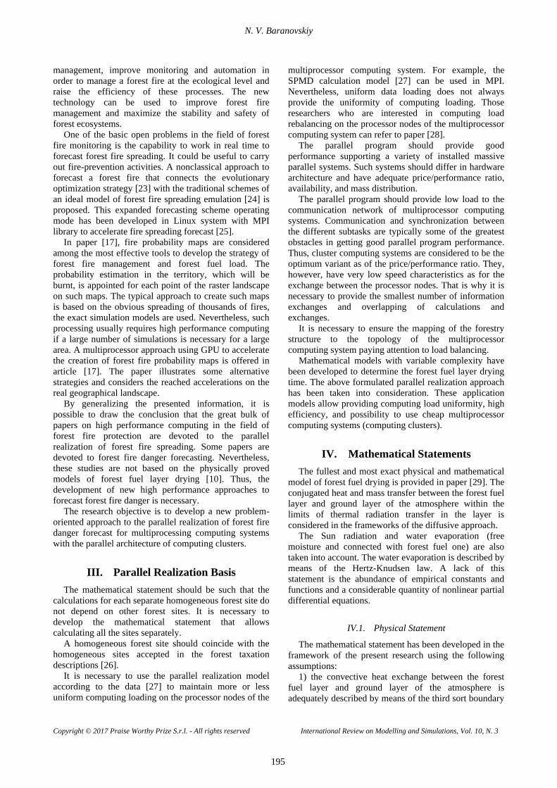
N. V. Baranovskiy
Copyright © 2017 Praise Worthy Prize S.r.l. - All rights reserved International Review on Modelling and Simulations, Vol. 10, N. 3
195
management, improve monitoring and automation in order to manage a forest fire at the ecological level and raise the efficiency of these processes. The new technology can be used to improve forest fire management and maximize the stability and safety of forest ecosystems.
One of the basic open problems in the field of forest fire monitoring is the capability to work in real time to forecast forest fire spreading. It could be useful to carry out fire-prevention activities. A nonclassical approach to forecast a forest fire that connects the evolutionary optimization strategy [23] with the traditional schemes of an ideal model of forest fire spreading emulation [24] is proposed. This expanded forecasting scheme operating mode has been developed in Linux system with MPI library to accelerate fire spreading forecast [25].
In paper [17], fire probability maps are considered among the most effective tools to develop the strategy of forest fire management and forest fuel load. The probability estimation in the territory, which will be burnt, is appointed for each point of the raster landscape on such maps. The typical approach to create such maps is based on the obvious spreading of thousands of fires, the exact simulation models are used. Nevertheless, such processing usually requires high performance computing if a large number of simulations is necessary for a large area. A multiprocessor approach using GPU to accelerate the creation of forest fire probability maps is offered in article [17]. The paper illustrates some alternative strategies and considers the reached accelerations on the real geographical landscape.
By generalizing the presented information, it is possible to draw the conclusion that the great bulk of papers on high performance computing in the field of forest fire protection are devoted to the parallel realization of forest fire spreading. Some papers are devoted to forest fire danger forecasting. Nevertheless, these studies are not based on the physically proved models of forest fuel layer drying [10]. Thus, the development of new high performance approaches to forecast forest fire danger is necessary.
The research objective is to develop a new problem-oriented approach to the parallel realization of forest fire danger forecast for multiprocessing computing systems with the parallel architecture of computing clusters.
III. Parallel Realization Basis The mathematical statement should be such that the
calculations for each separate homogeneous forest site do not depend on other forest sites. It is necessary to develop the mathematical statement that allows calculating all the sites separately.
A homogeneous forest site should coincide with the homogeneous sites accepted in the forest taxation descriptions [26].
It is necessary to use the parallel realization model according to the data [27] to maintain more or less uniform computing loading on the processor nodes of the
multiprocessor computing system. For example, the SPMD calculation model [27] can be used in MPI. Nevertheless, uniform data loading does not always provide the uniformity of computing loading. Those researchers who are interested in computing load rebalancing on the processor nodes of the multiprocessor computing system can refer to paper [28].
The parallel program should provide good performance supporting a variety of installed massive parallel systems. Such systems should differ in hardware architecture and have adequate price/performance ratio, availability, and mass distribution.
The parallel program should provide low load to the communication network of multiprocessor computing systems. Communication and synchronization between the different subtasks are typically some of the greatest obstacles in getting good parallel program performance. Thus, cluster computing systems are considered to be the optimum variant as of the price/performance ratio. They, however, have very low speed characteristics as for the exchange between the processor nodes. That is why it is necessary to provide the smallest number of information exchanges and overlapping of calculations and exchanges.
It is necessary to ensure the mapping of the forestry structure to the topology of the multiprocessor computing system paying attention to load balancing.
Mathematical models with variable complexity have been developed to determine the forest fuel layer drying time. The above formulated parallel realization approach has been taken into consideration. These application models allow providing computing load uniformity, high efficiency, and possibility to use cheap multiprocessor computing systems (computing clusters).
IV. Mathematical Statements The fullest and most exact physical and mathematical
model of forest fuel drying is provided in paper [29]. The conjugated heat and mass transfer between the forest fuel layer and ground layer of the atmosphere within the limits of thermal radiation transfer in the layer is considered in the frameworks of the diffusive approach.
The Sun radiation and water evaporation (free moisture and connected with forest fuel one) are also taken into account. The water evaporation is described by means of the Hertz-Knudsen law. A lack of this statement is the abundance of empirical constants and functions and a considerable quantity of nonlinear partial differential equations.
IV.1. Physical Statement
The mathematical statement has been developed in the framework of the present research using the following assumptions:
1) the convective heat exchange between the forest fuel layer and ground layer of the atmosphere is adequately described by means of the third sort boundary
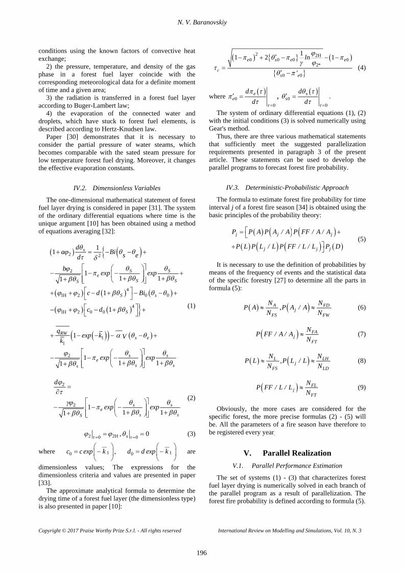
N. V. Baranovskiy
Copyright © 2017 Praise Worthy Prize S.r.l. - All rights reserved International Review on Modelling and Simulations, Vol. 10, N. 3
196
conditions using the known factors of convective heat exchange;
2) the pressure, temperature, and density of the gas phase in a forest fuel layer coincide with the corresponding meteorological data for a definite moment of time and a given area;
3) the radiation is transferred in a forest fuel layer according to Buger-Lambert law;
4) the evaporation of the connected water and droplets, which have stuck to forest fuel elements, is described according to Hertz-Knudsen law.
Paper [30] demonstrates that it is necessary to consider the partial pressure of water steams, which becomes comparable with the sated steam pressure for low temperature forest fuel drying. Moreover, it changes the effective evaporation constants.
IV.2. Dimensionless Variables
The one-dimensional mathematical statement of forest fuel layer drying is considered in paper [31]. The system of the ordinary differential equations where time is the unique argument [10] has been obtained using a method of equations averaging [32]:
2 2
2
41 2 0 0
41 2 0 0
11
2
11
11 11
1
1
1
11 11
s
S Se
S SS
S s
S
RWs e
s se
ss
da Bi s ed
b exp exp
c d Bi
c d
______q
exp k Vk
exp exp
s
(1)
2
2 11 11
s se
s sS
d
exp exp
(2)
2 20 0 0s, (3)
where 10
__c c exp k
, 10
__d d exp k
are
dimensionless values; The expressions for the dimensionless criteria and values are presented in paper [33].
The approximate analytical formula to determine the drying time of a forest fuel layer (the dimensionless type) is also presented in paper [10]:
2 20 0 0 0
2
0 0
11 2 1e s e e*
сs e
ln
'
(4)
where
00
ee
dd
, 0
0
ss
dd
.
The system of ordinary differential equations (1), (2) with the initial conditions (3) is solved numerically using Gear's method.
Thus, there are three various mathematical statements that sufficiently meet the suggested parallelization requirements presented in paragraph 3 of the present article. These statements can be used to develop the parallel programs to forecast forest fire probability.
IV.3. Deterministic-Probabilistic Approach
The formula to estimate forest fire probability for time interval j of a forest fire season [34] is obtained using the basic principles of the probability theory:
j j j
j j j
P P A P A / A P FF / A / A
P L P L / L P FF / L / L P D
(5)
It is necessary to use the definition of probabilities by
means of the frequency of events and the statistical data of the specific forestry [27] to determine all the parts in formula (5):
A FDj
FS FW
N NP A ,P A / AN N
(6)
FAj
FT
NP FF / A / AN
(7)
L LHj
FS LD
N NP L ,P L / LN N
(8)
FLj
FT
NP FF / L / LN
(9)
Obviously, the more cases are considered for the
specific forest, the more precise formulas (2) - (5) will be. All the parameters of a fire season have therefore to be registered every year.
V. Parallel Realization V.1. Parallel Performance Estimation
The set of systems (1) - (3) that characterizes forest fuel layer drying is numerically solved in each branch of the parallel program as a result of parallelization. The forest fire probability is defined according to formula (5).
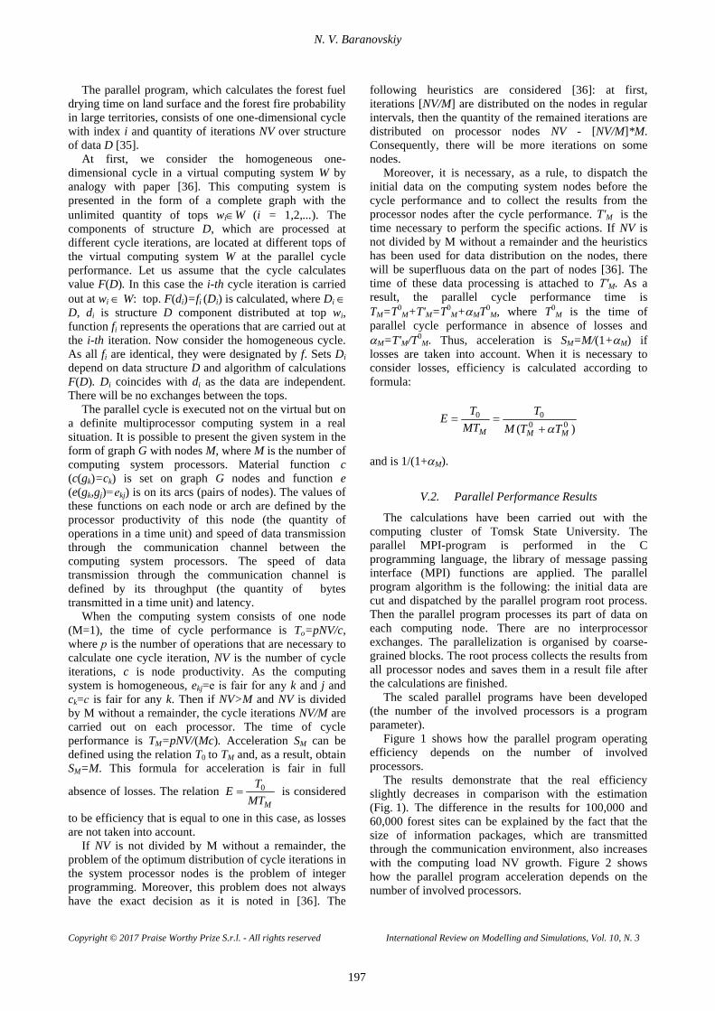
N. V. Baranovskiy
Copyright © 2017 Praise Worthy Prize S.r.l. - All rights reserved International Review on Modelling and Simulations, Vol. 10, N. 3
197
The parallel program, which calculates the forest fuel drying time on land surface and the forest fire probability in large territories, consists of one one-dimensional cycle with index i and quantity of iterations NV over structure of data D [35].
At first, we consider the homogeneous one-dimensional cycle in a virtual computing system W by analogy with paper [36]. This computing system is presented in the form of a complete graph with the unlimited quantity of tops wiW (i = 1,2,...). The components of structure D, which are processed at different cycle iterations, are located at different tops of the virtual computing system W at the parallel cycle performance. Let us assume that the cycle calculates value F(D). In this case the i-th cycle iteration is carried out at wi W: top. F(di)=fi (Di) is calculated, where Di D, di is structure D component distributed at top wi, function fi represents the operations that are carried out at the i-th iteration. Now consider the homogeneous cycle. As all fi are identical, they were designated by f. Sets Di depend on data structure D and algorithm of calculations F(D). Di coincides with di as the data are independent. There will be no exchanges between the tops.
The parallel cycle is executed not on the virtual but on a definite multiprocessor computing system in a real situation. It is possible to present the given system in the form of graph G with nodes M, where M is the number of computing system processors. Material function c (c(gk)=ck) is set on graph G nodes and function e (e(gk,gj)=еkj) is on its arcs (pairs of nodes). The values of these functions on each node or arch are defined by the processor productivity of this node (the quantity of operations in a time unit) and speed of data transmission through the communication channel between the computing system processors. The speed of data transmission through the communication channel is defined by its throughput (the quantity of bytes transmitted in a time unit) and latency.
When the computing system consists of one node (M=1), the time of cycle performance is To=pNV/c, where р is the number of operations that are necessary to calculate one cycle iteration, NV is the number of cycle iterations, c is node productivity. As the computing system is homogeneous, ekj=е is fair for any k and j and ck=с is fair for any k. Then if NV>M and NV is divided by M without a remainder, the cycle iterations NV/M are carried out on each processor. The time of cycle performance is TM=pNV/(Mc). Acceleration SM can be defined using the relation T0 to TM and, as a result, obtain SM=M. This formula for acceleration is fair in full
absence of losses. The relation MMT
TE 0 is considered
to be efficiency that is equal to one in this case, as losses are not taken into account.
If NV is not divided by M without a remainder, the problem of the optimum distribution of cycle iterations in the system processor nodes is the problem of integer programming. Moreover, this problem does not always have the exact decision as it is noted in [36]. The
following heuristics are considered [36]: at first, iterations [NV/M] are distributed on the nodes in regular intervals, then the quantity of the remained iterations are distributed on processor nodes NV - [NV/M]*M. Consequently, there will be more iterations on some nodes.
Moreover, it is necessary, as a rule, to dispatch the initial data on the computing system nodes before the cycle performance and to collect the results from the processor nodes after the cycle performance. T'M is the time necessary to perform the specific actions. If NV is not divided by M without a remainder and the heuristics has been used for data distribution on the nodes, there will be superfluous data on the part of nodes [36]. The time of these data processing is attached to Т'M. As a result, the parallel cycle performance time is TM=T0
M+T'M=T0M+MT0
M, where T0M is the time of
parallel cycle performance in absence of losses and M=T'M/T0
M. Thus, acceleration is SM=M/(1+M) if losses are taken into account. When it is necessary to consider losses, efficiency is calculated according to formula:
)( 00
00
MMM TTMT
MTTE
and is 1/(1+M).
V.2. Parallel Performance Results
The calculations have been carried out with the computing cluster of Tomsk State University. The parallel MPI-program is performed in the C programming language, the library of message passing interface (MPI) functions are applied. The parallel program algorithm is the following: the initial data are cut and dispatched by the parallel program root process. Then the parallel program processes its part of data on each computing node. There are no interprocessor exchanges. The parallelization is organised by coarse-grained blocks. The root process collects the results from all processor nodes and saves them in a result file after the calculations are finished.
The scaled parallel programs have been developed (the number of the involved processors is a program parameter).
Figure 1 shows how the parallel program operating efficiency depends on the number of involved processors.
The results demonstrate that the real efficiency slightly decreases in comparison with the estimation (Fig. 1). The difference in the results for 100,000 and 60,000 forest sites can be explained by the fact that the size of information packages, which are transmitted through the communication environment, also increases with the computing load NV growth. Figure 2 shows how the parallel program acceleration depends on the number of involved processors.

N. V. Baranovskiy
Copyright © 2017 Praise Worthy Prize S.r.l. - All rights reserved International Review on Modelling and Simulations, Vol. 10, N. 3
198
Fig. 1. Parallel program efficiency depending on number of processors for 100,000 and 60,000 homogenous sites
Fig. 2. Acceleration of parallel program depending on number of processors for 100,000 homogenous sites
In a real situation, acceleration is a slightly less than
the one obtained by the estimation without losses because the time share is lost during data dispatch at the beginning and during results gathering at the end of the parallel program performance. It appears that acceleration decreases when the number of processors increases, though the computing load on each processor decreases. Nevertheless, the time the root process spends to interact with other processes for data dispatch and gathering increases. The high-speed indicators of the computing cluster communication environment are not large, and the architectural aspects play a role here.
Having analyzed the obtained results, the conclusion is that the considered problem algorithm fits very well with the parallel realization by means of multiprocessor computing systems. Acceleration is virtually proportional to the number of involved processors. Efficiency does not always depend on the number of involved processors as there are no interprocessor data transmissions in the program work. It is established that the loss of performance is insignificant and
1160 09MM ,
max ,
.
It should be noted that despite the application of heuristics to distribute data in a case, when NV is not divided by M without a remainder (the static heuristics with preliminary distribution before the parallel cycle beginning), it does not result in an appreciable misbalance of computing load. Consequently, there is no necessity to apply the dynamic rebalancing of computing
load during the parallel program performance. The root process of the parallel program dispatches and gathers data by means of the vector variants of dispatch and gathering functions from MPI library.
V.3. Forest Fire Danger Estimation Results
The forest fire conditions are related to the Timiryazevskiy forestry, in Tomsk region [26]. The anthropogenic load is considered to be maximal. As the small territory of Timiryazevskiy forestry is considered, we show the influence of meteorological conditions on the integrated estimation of forest fire danger by varying the precipitation amount. Table I shows the data on a precipitation factor depending on the precipitation amount to calculate forest fire probability according to the meteorological conditions.
TABLE I
FACTOR OF PRECIPITATION [37] Precipi- tation, mm
No 0.1–0.9
1.0–2.9
3.0–5.9
6.0–14.9
15.0–19.9
20 and
more kh 1.0 0.8 0.6 0.4 0.2 0.1 0.0
To be precise, it was considered that there were 0, 0.5,
1.5, 4.0, 15 mm of precipitation in the territories of Timiryazevskiy, Moryakovskiy, Bogorodskiy, Kireevskiy, and Zhukovskiy local forestries, respectively. Figure 3 shows the forest fire probability in the territory of the specific forestry and timber enterprise. The local forestries are designated by figures: 1 - Timiryazevskiy, 2 - Moryakovskiy, 3 - Bogorodskiy, 4 - Kireevskiy, 5 – Zhukovskiy. Line 6 designates the forest fire probability for a forestry as a whole.
Fig. 3. Probability of forest fire on Saturday depending on time for specific local forestry and timber enterprise (meteorological conditions)
The influence of anthropogenic load on the forest fire
probability has been analyzed. The scenario corresponds to the forest fire conditions of Timiryazevskiy forestry in Tomsk region [26]. The data on the probable presence of fire sources P(Aj/A) in Timiryazevskiy forestry are presented in Table II. Figure 4 shows the forest fire probability in various days of the week.
The storm activity influence on the forest fire danger level has been analysed. Table III shows the data on the probability of a cloud-to-ground lightning discharge.
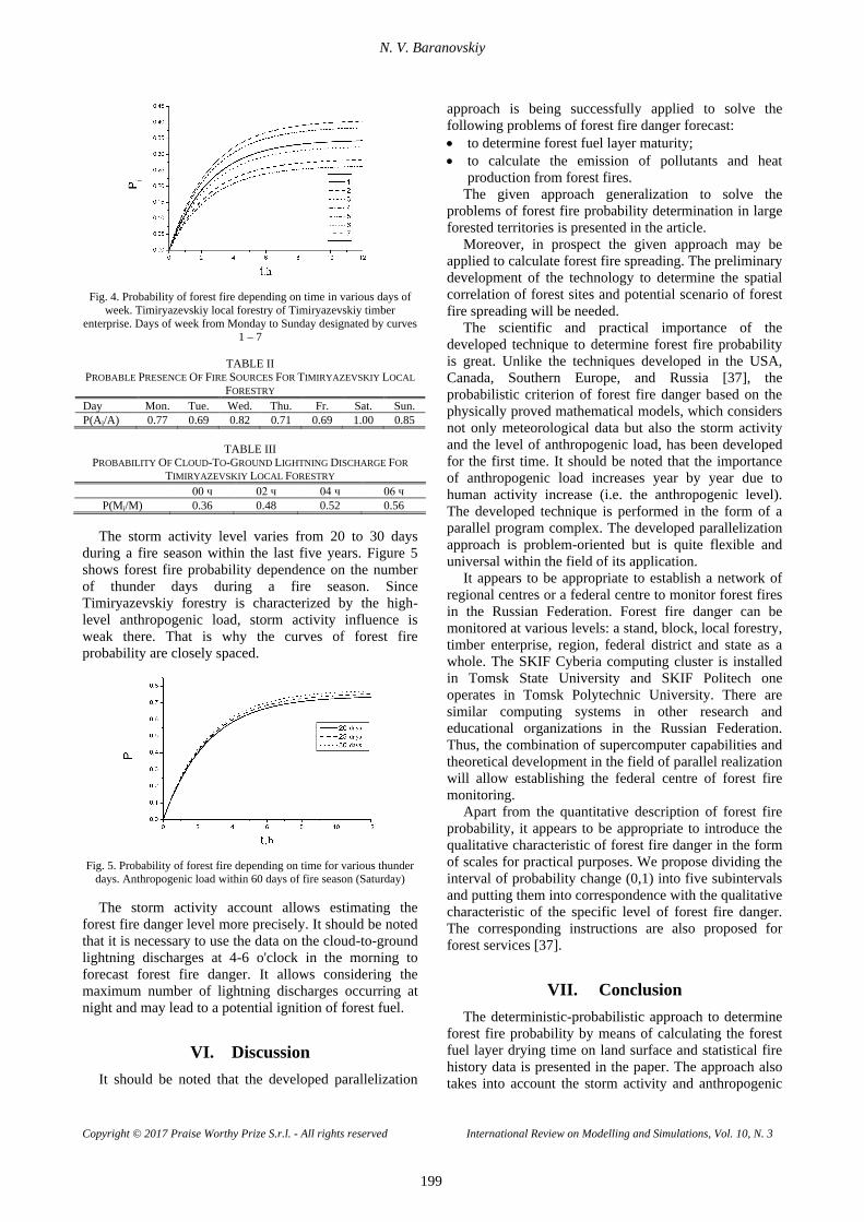
N. V. Baranovskiy
Copyright © 2017 Praise Worthy Prize S.r.l. - All rights reserved International Review on Modelling and Simulations, Vol. 10, N. 3
199
Fig. 4. Probability of forest fire depending on time in various days of week. Timiryazevskiy local forestry of Timiryazevskiy timber
enterprise. Days of week from Monday to Sunday designated by curves 1 – 7
TABLE II
PROBABLE PRESENCE OF FIRE SOURCES FOR TIMIRYAZEVSKIY LOCAL FORESTRY
Day Mon. Tue. Wed. Thu. Fr. Sat. Sun. P(Aj/A) 0.77 0.69 0.82 0.71 0.69 1.00 0.85
TABLE III
PROBABILITY OF CLOUD-TO-GROUND LIGHTNING DISCHARGE FOR TIMIRYAZEVSKIY LOCAL FORESTRY
00 ч 02 ч 04 ч 06 ч P(Mj/M) 0.36 0.48 0.52 0.56
The storm activity level varies from 20 to 30 days
during a fire season within the last five years. Figure 5 shows forest fire probability dependence on the number of thunder days during a fire season. Since Timiryazevskiy forestry is characterized by the high-level anthropogenic load, storm activity influence is weak there. That is why the curves of forest fire probability are closely spaced.
Fig. 5. Probability of forest fire depending on time for various thunder days. Anthropogenic load within 60 days of fire season (Saturday)
The storm activity account allows estimating the
forest fire danger level more precisely. It should be noted that it is necessary to use the data on the cloud-to-ground lightning discharges at 4-6 o'clock in the morning to forecast forest fire danger. It allows considering the maximum number of lightning discharges occurring at night and may lead to a potential ignition of forest fuel.
VI. Discussion It should be noted that the developed parallelization
approach is being successfully applied to solve the following problems of forest fire danger forecast: to determine forest fuel layer maturity; to calculate the emission of pollutants and heat
production from forest fires. The given approach generalization to solve the
problems of forest fire probability determination in large forested territories is presented in the article.
Moreover, in prospect the given approach may be applied to calculate forest fire spreading. The preliminary development of the technology to determine the spatial correlation of forest sites and potential scenario of forest fire spreading will be needed.
The scientific and practical importance of the developed technique to determine forest fire probability is great. Unlike the techniques developed in the USA, Canada, Southern Europe, and Russia [37], the probabilistic criterion of forest fire danger based on the physically proved mathematical models, which considers not only meteorological data but also the storm activity and the level of anthropogenic load, has been developed for the first time. It should be noted that the importance of anthropogenic load increases year by year due to human activity increase (i.e. the anthropogenic level). The developed technique is performed in the form of a parallel program complex. The developed parallelization approach is problem-oriented but is quite flexible and universal within the field of its application.
It appears to be appropriate to establish a network of regional centres or a federal centre to monitor forest fires in the Russian Federation. Forest fire danger can be monitored at various levels: a stand, block, local forestry, timber enterprise, region, federal district and state as a whole. The SKIF Cyberia computing cluster is installed in Tomsk State University and SKIF Politech one operates in Tomsk Polytechnic University. There are similar computing systems in other research and educational organizations in the Russian Federation. Thus, the combination of supercomputer capabilities and theoretical development in the field of parallel realization will allow establishing the federal centre of forest fire monitoring.
Apart from the quantitative description of forest fire probability, it appears to be appropriate to introduce the qualitative characteristic of forest fire danger in the form of scales for practical purposes. We propose dividing the interval of probability change (0,1) into five subintervals and putting them into correspondence with the qualitative characteristic of the specific level of forest fire danger. The corresponding instructions are also proposed for forest services [37].
VII. Conclusion The deterministic-probabilistic approach to determine
forest fire probability by means of calculating the forest fuel layer drying time on land surface and statistical fire history data is presented in the paper. The approach also takes into account the storm activity and anthropogenic

N. V. Baranovskiy
Copyright © 2017 Praise Worthy Prize S.r.l. - All rights reserved International Review on Modelling and Simulations, Vol. 10, N. 3
200
load in the controlled territories. To calculate the forest fuel drying time, it is required
to know its current moisture content in a controlled forest area [10]. Field observations and measurements are possible only near populated areas and mobile forest guard posts. The most suitable option is the use of indirect methods for estimating the initial moisture content, taking into account precipitation and the meteorological characteristics available in meteostation statistics. The network of meteostantions is inconsiderable in Russia compared to networks in Canada, the United States and Europe. This is especially true for the territories of Siberia and the Far East. Therefore, a methodology for estimating the initial moisture content using satellite data on the surface atmosphere layer from the MODIS Terra/Aqua platform is currently being developed [38].
The Canadian system provides good results despite the lack of physically sound components. However, in the case of sharp climatic changes, the technique proposed in this article can give a much more accurate prediction of forest fire danger. It should be noted that there is no need to develop a completely new system for forecasting forest fire danger, for example, in Russia. Now, in Russia ISDM-Rosleskhoz is operated [9]. This system includes information on current forest fires, weather station data, forest fire statistics for anthropogenic reasons and thunderstorm activity. The data of lightning location are available in the system. It will be sufficient to organize the loading of data from the cluster for visualization into ISDM-Rosleskhoz. In addition, to assess the probability of lightning-caused forest fires, the WWLLN data available to network participants in real time can be used [39]. Both Canadian and American methods can be easily modernized by using a probabilistic criterion in conjunction with FWI [8].
The new problem-oriented approach to parallel realization has been developed. The research results demonstrate that the approach is very effective to solve the problems of forest fuel layer fire maturity and forest fire probability determination. The parallel program almost reaches the maximum possible acceleration when the acceleration is virtually proportional to the number of involved processors.
A distinctive feature of the presented approach is the use of an independent calculation of the forest fuel drying time for each homogeneous forest area. This ensures that the code runs on all processors without exchanges during the computation process. As a result, the acceleration of the parallel program is close to the theoretical limit.
The deterministic-probabilistic approach to determine forest fire probability and the considered parallel realization approach allow developing very effective parallel programs to forecast the forest fire danger in large forested territories. The approach test implementation was performed in Timiryazevskiy forestry in Tomsk region. In conclusion, the integration
of the parallel program complex to forecast forest fire danger and the geoinformation system to estimate forest fire danger [40-42] is possible.
Acknowledgements This work was supported by the Russian Foundation
for Basic Research and Administration of Tomsk region. Grant N 16-41-700831.
The Author thanks the Interregional Supercomputing Center of Tomsk State University. The computing experiments have been carried out by the SKIF Cyberia multiprocessor cluster.
References [1] A.M. Grishin, Mathematical modelling of forest fires and new
methods of fighting them (Publishing House of the Tomsk State University, 1997)
[2] А.М. Grishin, Physics of forest fires, (Publishing house TGU, 1994) (In Russian)
[3] A.S. Isaev, G.N. Korovin, S.P. Titov at al., Environmental problems of absorption of carbonic gas by means of forest recovery and forestation in Russia: State-of-the-art review, (Center of ecological policy, 1995) (In Russian)
[4] M.E. Alexander, B.J. Stocks, B.D. Lawson, The Canadian forest fire danger rating system, Initial Attack, Spring: 6-9. 1996.
[5] R.E. Burgan, 1988 Revisions to the 1978 National Fire-Danger Rating System. Research Paper SE-273. (Asheville, NC: Southeastern Forest Experiment Station, Forest Service, U.S. Department of Agriculture, 1988)
[6] A. Camia, P. Barbosa, G. Amatulli, J. San-Miguel-Ayanz, Fire danger rating in the European Forest Fire Information System (EFFIS): Current developments, Forest Ecology and Management. Vol. 234 (suppl. 1): S20. 2006.
[7] D.X. Viegas, G. Bovio, A. Ferreira et al., Comparative study of various methods of fire danger evaluation in Southern Europe, International Journal of Wildland Fire. Vol. 10: 235-246. 1999.
[8] D.L. Martell, A Markov chain model of day to day changes in the Canadian Forest Fire Weather Index, International Journal of Wildland Fire. Vol. 9: 265-273. 1999.
[9] E.A. Loupian, S.A. Bartalev, D.V. Ershov et al., Satellite data processing management in Forest Fires Remote Monitoring Information System (ISDM-Rosleskhoz) of the Federal Agency for Forestry, Sovremennye Problemy Distantsionnogo Zondirovaniya Zemli iz Kosmosa, Vol. 12: 222-250. 2015.
[10] A.M. Grishin, N.V. Baranovskii, Comparative Analysis of Simple Models of Drying of the Forest Combustibles, Including the Data of Experiments and Natural Observations, Journal of Engineering Physics and Thermophysics. Vol. 76 (Issue 5): 166-169. 2003.
[11] S.W. Taylor, M.E. Alexander, Science, technology and human factors in fire danger rating: the Canadian experience, International Journal of Wildland Fire. Vol. 15: 121-135. 2006.
[12] A.M. Grishin, S.P. Sinitsyn, I.V. Akimova, Comparative analysis of the thermokinetic constants for drying and pyrolyzing forest fuels, Combustion, Explosion, and Shock Waves, Vol. 27: 663-669. 1991.
[13] V.V. Falfushinsky, Parallel processing of multicomponent seismic data, Cybernetics and Systems Analysis, Vol. 47 (Issue 2): 330-334. 2011.
[14] R. Rodriguez, A. Cortes, T. Margalef, Data injection at execution time in Grid environments using Dynamic Data Dryven Application System for wildland fire spread prediction, 2010 10th IEEE/ACM International Conference on Cluster, Cloud and Grid Computing. pp. 565-568. 2011.
[15] J. Tang, T. Gong, J. Zhou, Research on anti-forest-fire ecological management system with cloud-computing, 2011 7th International Conference on Natural Computation. pp. 2241-2245. 2011.
[16] B. Abdalhaq, A. Cortes, T. Margalef, G. Bianchini, E. Luque,

N. V. Baranovskiy
Copyright © 2017 Praise Worthy Prize S.r.l. - All rights reserved International Review on Modelling and Simulations, Vol. 10, N. 3
201
Between classical and ideal: enhancing wildland fire prediction using cluster computing, Cluster Computing, Vol. 9: 329-343. 2006.
[17] D. D’Ambrosio, S. Di Gregorio, G. Filippone, R. Rongo, W. Spataro, G.A., A Multi-GPU Approach to Fast Wildfire Hazard Mapping, Simulation and Modeling Methodologies, Technologies and Applications. Advances in Intelligent Systems and Computing, Vol. 256: 183-195. 2014.
[18] F. Darema, Grid computing and beyond: the context of dynamic data driven applications systems, Proceedings of the IEEE, Vol. 93 (Issue 3): 692-697. 2005.
[19] M. Denharm, A. Cortes, T. Margalef, E. Luque, Applying a Dynamic Data Driven Genetic Algorithm to improve forest fire spread prediction, Lecture Notes in Computer Science, Vol. 5103: 36-45. 2008.
[20] J. Tang, Research on Cloud Computing, Journal of Inner Mongolia University for Nationalities, Vol. 16 (Issue 2): 15-16. 2010.
[21] R.N. Calheiros, R. Ranjan, A. Beloglazov et al., CloudSim: A toolkit for modelling and simulation of Cloud Computing environments and evaluation of resource provisioning algorithms, Software: Practice and Experience, Vol. 41 (Issue 1): 23-50. 2011.
[22] Sh. Wei, Sh. Wei, Analysis on traditional forest fire prevention and path selection on modern forest fire ecology management, Forest Fire Prevention, (Issue 4): 6-11. 2009.
[23] B. Abdalhaq, A. Cortes, T. Margalef, E. Luque, Evolutionary optimisation techniques on computational grids, Lecture Notes in Computer Science, Vol. 2329: 513-522. 2002.
[24] M.A. Finney, FARSITE: Fire area simulator model development and evaluation. Research Report RMRS-RP-4 (USDA Forest Service, 1998).
[25] M. Snir, S.M. Otto, S. Huss-Lederman, D. Walker, J. Dongarra, MPI: The Complete Reference (MIT Press, 1996).
[26] The project of the organisation and development of Timiryazevskiy forestry of Tomsk timber territorial production association of the ministry of a forestry of RSFSR. Volume III. Forest taxation descriptions of the Timiryazevsky forestry (Gosleshoz USSR. All-union association "Lesproject". Western-Siberian timber enterprise, 1990) (In Russian)
[27] J. Xue, SPMD Code Generation, The Springer International Series in Engineering and Computer Science, Vol. 575 Loop Tiling for Parallelism: 123-168. 2000.
[28] A.V. Plastino, D. Vianna, R. Costa, O.T. da Silveira Filho, Load Balancing in SPMD Applications: Concepts and Experiments, The Springer International Series in Engineering and Computer Science. Vol. 750 High Performance Scientific and Engineering Computing: 95-107. 2004.
[29] A.M. Grishin, A.N. Golovanov, L.Yu. Kataeva, E.L. Loboda, Formulation and Solution of the Problem of Drying of a Layer of Combustible Forest Materials, Combustion, Explosion, and Shock Waves, Vol. 37: 57-66. 2001.
[30] A.M. Grishin, A.N. Golovanov, S.V. Rusakov, Evaporation of free water and water bound with forest combustibles under isothermal conditions, Journal of Engineering Physics and Thermophysics, Vol. 76: 1166-1172. 2003.
[31] E.L. Loboda, Physical and mathematical modelling of drying and ignition of forest fuel layer, PhD Dissertation, Dept. Phys. and Comp. Mech., Tomsk State University, Tomsk, 2002. (In Russian)
[32] A.I. Volpert, S.I. Hudyaev, Analys in classes of discontinuous functions and the equations of mathematical physics (Science, 1975) (In Russian)
[33] A.M. Grishin, A.N. Golovanov, L.Yu. Kataeva, E.L. Loboda, Problem of drying of a layer of combustible forest materials, Journal of Engineering Physics and Thermophysics, Vol. 74: 919-928. 2001.
[34] N.V. Baranovskiy, M.V. Zharikova, A Web-Oriented Geoinformation System Application for Forest Fire Danger Prediction in Typical Forests of the Ukraine, Lecture Notes in Geoinformation and Cartography. Thematic Cartography for the Society: 13-22. 2014.
[35] E.V. Adutskevich, N.A. Likhoded, A.O. Sikorsky, Parallelization of sequential programs: distribution of arrays among processors
and structurization of communications, Cybernetics and Systems Analysis, Vol. 48 (Issue 1): 122-137. 2012.
[36] A.I. Avetisyan, S.S. Gaisaryan, O.I. Samovarov, Possibilities of Optimal Execution of Parallel Programs Containing Simple and Iterated Loops on Heterogeneous Parallel Computational Systems with Distributed Memory, Programming and Computer Software, Vol. 28: 28-40. 2002.
[37] G.V. Kuznetsov, N.V. Baranovskiy, Forecast of forest fire occurrence and their ecological consequences (Publishing house of the Siberian Branch of the Russian Academy of Science, 2009) (In Russian)
[38] S. Seemann, J. Li, W.P. Menzel, L. Gumley, Operational retrieval of atmospheric temperature, moisture, and ozone from MODIS infrared radiances, Journal of Applied Meteorology, Vol. 42: 1072-1091. 2003.
[39] V. Bui, L.-C. Chang, S. Heckman, A performance study of earth networks total lighting network (ENTLN) and worldwide lightning location network (WWLLN), Proceedings - 2015 International Conference on Computational Science and Computational Intelligence, CSCI 2015, paper N 7424122, pp. 386-391. Las Vegas. 2016.
[40] E.P. Yankovich, N.V. Baranovskiy, K.S. Yankovich, ArcGIS for assessment and display of the probability of forest fire danger, 2014 9th International Forum on Strategic Technology, IFOST 2014, pp. 222–225. 2014.
[41] N.V. Baranovskiy, E.P. Yankovich, Estimation and mapping of forest fire danger by action of the focused sunlight in geographical information system, Proceedings of 5th International Conference on Cartography and GIS, Vol. 2, pp. 756–762, Riviera, 2014.
[42] E.P. Yankovich, N.V. Baranovskiy, Forest taxation data geoprocessing for assessment of forest fire danger caused by focused sunlight, 14th International Multidisciplinary Scientific Geoconference SGEM - 2014. GeoConference on Informatics, Geoinformatics and Remote Sensing, Vol. 1, pp. 607–612, Albena, 2014.
[43] A.M. Grishin, N.V. Baranovskii, Comparative Analysis of Simple Models of Drying of the Forest Combustibles, Including the Data of Experiments and Natural Observations, Journal of Engineering Physics and Thermophysics. Vol. 76 (Issue 5): 166-169. 2003.
[44] D.A. Franc-Kamenetsky, Diffusion and heat transfer in chemical kinetics (Science, 1987) (In Russian)
Authors’ information National Research Tomsk Polytechnic University, Tomsk.
Nikolay Baranovskiy received the Specialist Degree in Mechanics from Tomsk State University in 2000. He received the PhD Degree in Physics and Mathematics from Tomsk State University in 2007. His current position is Associate Professor at Tomsk Polytechnic University. His current interests include forest fire danger and ecological impact prediction,
parallel computing and spatial data analysis using GIS and RS technologies. Dr. Baranovskiy is a Member of the International Association of Wildland Fire and of the International Association of Engineers.

International Review on Modelling and Simulations (I.RE.MO.S.), Vol. 10, N. 3
ISSN 1974-9821 June 2017
Copyright © 2017 Praise Worthy Prize S.r.l. - All rights reserved https://doi.org/10.15866/iremos.v10i3.11479
202 202 202
Rule-Based and Genetic Algorithm for Automatic Gamelan Music Composition
Khafiizh Hastuti1,2, Azhari1, Aina Musdholifah1, Rahayu Supanggah3 Abstract – This research aims to develop a system of automatic gamelan music composition. Gamelan is the traditional ensemble music of Java, Indonesia. The authors propose a model of automatic gamelan music composition which consists of knowledge, rules, and random generation. There are three types of knowledge, basic, construction, and melodic knowledge. The basic knowledge contains the general knowledge of gamelan music. The construction knowledge controls the components building a composition. The melodic knowledge controls quality of the sound. The knowledge is transformed into rules of notes arrangement used to produce the characteristic sound of gamelan music. Genetic algorithm is used to generate a composition. Gatra, the smallest unit in a composition that contains four beats (notes), is used as a variable to construct the genes of a chromosome. The fitness value is measured based on the weight of notes distribution, identical gatras and melodic features. The evaluation is conducted to measure the quality of sound of “ladrang laras slendro pathet manyura” composition created by the system. The evaluation is conducted based on Turing test which involves human experts to recognize the composition created by the system. The results show that the model of automatic gamelan music composition proposed in this research is effective. All the gamelan experts state that it is very difficult to find the differences between the composition created by the system when it is randomly arranged and other compositions created by humans. 4 out of 6 gamelan experts failed to recognize a composition created by the system. Copyright © 2017 Praise Worthy Prize S.r.l. - All rights reserved. Keywords: Rule-Based, Genetic Algorithm, Gamelan Music, Automatic Music Composition
Nomenclature A-B-C-D Concept of gatra Balungan Composition skeleton Gamelan Traditional music ensemble Gatra The smallest unit of gamelan music Gending Gamelan song Laras Musical scale in gamelan music which
consists of slendro and pelog Pathet A system of categorizing the use of tones Pin Dot notation Rasa Sensation or inner mining or ability to
express or perceive feeling Ricikan Gamelan instrument ND Number of notes distribution P Data partition S Sequence TF Total number of functions TN Total number of notes TS Total number of itemsets in a sequence WC Weight chaining WN Weight distribution
I. Introduction Computer music is created using computer technology
for artistic conception. It is a subject studied in artificial intelligence researches and ongoing experiments, both on computer music created entirely using computer and with the help of computers [1] [2].
The use of artificial intelligence in music composition is known as algorithmic composition, where certain algorithms are used to automatically create a music composition. Algorithmic composition is a field of research in computer music which studies the process of automatic music composition by partially or wholly using computer; The algorithmic composition software is programmed to generate music with a certain autonomy [3] [4]. The Algorithmic composition started with the works on Illiac Suite and Xenakis. Illiac Suite, developed by [5], uses the rule-based method, and Xenakis, developed by [6], uses Markov models. The algorithmic composition has grown in many variants of algorithmic approaches, such as generative grammars, Genetic Algorithm, cellular automata, neural networks, machine-learning techniques, expert systems, and others [3] [7] [8].
In this research, the algorithmic composition is used for the traditional ensemble music of Java, Indonesia, called gamelan music. Gamelan music has elements of aesthetic, intellectual, beliefs, customs, order, works of human creativity, nature, rules of life, welfare, and

Khafiizh Hastuti, Azhari, Aina Musdholifah, Rahayu Supanggah
Copyright © 2017 Praise Worthy Prize S.r.l. - All rights reserved International Review on Modelling and Simulations, Vol. 10, N. 3
203
society; hence it cannot be separated from human, humanity, and God [9]. Gamelan music uses gamelan as an instrument for orchestra or ensemble music, and gending as the composition of the song [10]. Gending is a general term used to refer to Javanese gamelan music composition [11]. Gamelan melodies are bound by rules and regulations (Javanese society), which are sacred [12]. The process of creating gamelan music should consider the Javanese musical concept, because gamelan is not only the mean of performances, but also a part of the Javanese community life, including the concept of cosmology and other concepts of life [13].
In this research, the rule-based and Genetic algorithm approaches are used for automatic gamelan music composition. Knowledge of gamelan music composition is transformed into rules for automatic composition, and Genetic algorithm is used to arrange notes sequences for composition. Some works on Western ensemble music were CHORAL and Bach in Box. The rule-based system was used by [14] to develop CHORAL, a system for the harmonization of four-part chorales in J.S. Bach’ style. The use of rules as constraints in generating composition with the Genetic algorithm was used in Bach in Box developed by [15].
Gamelan music is different from Western music. Gatra is the smallest unit of gamelan music composition which contains four beats, and each beat can be a note or pin (dot notation). The notes sequence arrangement in gatra is the characteristic of gamelan music sound. Gatra was analyzed by [16] and [17] to formalize certain types of gending. The grammar approach is used by [16] to identify the contour of gatra with srepegan, a type of gending, as the subject of the research. The contour is defined based on pitch scale (higher and lower notes) of notes sequence in a gatra. The structure of gamelan music called gending lampah is studied using a quasi-linguistic approach [17].
The authors of this paper proposed to use the sequential pattern mining technique to analyze the notes sequences of gatra. In a previous work [18], they developed a new sequential pattern mining algorithm called AFiS to formalize the melodic feature of gamelan music. The development of AFiS algorithm, which will be discussed later in this paper, was inspired by the philosophical concept at the base of arranging notes sequences of gatra.
II. Related Works Computer music is created using computer technology
for artistic conception. It is a subject studied in artificial intelligence researches and ongoing experiments, both on computer music created entirely using computer and with the help of computers [1] [2]. CHORAL is an expert system for the harmonization of four-part chorales in J.S. Bach’s style. The system uses more than 270 rules to produce multi-view points, such as skeleton, individual melodic lines for each sound, and schenkerian voice leading in descant and bass [14]. Bach in Box uses rules
defined by musical scholars, including a pre-defined melody, to control the search space for four-part baroque harmony [15]. Bach in Box uses the Genetic algorithm to generate the composition. Its fitness is measured based on the basis chords, ranges, motion, harmonic interest, beginning and end chords, smoothness and resolution.
The unsupervised learning approach based on a corpus of jazz musical performances is used by implementing a combination of clustering technique and Markov chains. The K-means algorithm is used to statistically collect data in a corpus, and then the data are used as statement in Markov Chain [19]. The Lindenmayer technique is used to generate a composition based on simple inputs from users, and then the input is developed using the probability model, fractal, and chaos [20]. The grammar approach is used to develop ImprovGenerator, a system which learns the percussion pattern in live-streaming, and generates accompaniment tracks in real time. The mixed model including a hierarchy structure representing a stochastic context-free grammar is then used to generate patterns of accompaniment music based on history and temporary patterns. The transition probability model is used to improve the generated grammar patterns [21].
Genetic algorithm is used to generate multi-instrumental, guitar-oriented rock music. A unique conversion procedure from numerical values to abc language, and from abc language to numerical values allows combination of optimization number with variants expression from musical description language. The abc language is used to notate music in the ASCII format, and converts a song notated in this language into MIDI format by program [22]. The operators of the Genetic algorithm are modified by [23] to allow pitch schedule and interlude changing significantly. The approach includes a pre-defined rhythm which is set as the initial population. A program developed by [24] is designed to create original music compositions based on rules and musical theory. The parameters of the composition, preferences of genre, tempo, and tone, are controlled by the user, and the Genetic algorithm is used to generate a composition.
III. Proposed Model In this research, the authors revised their previous
proposed model of automatic gamelan music composition [25]. During their experiments, they developed a new algorithm called AFiS (A priori based on Functions in sequence) to identify sequential patterns, and gamelan notes pattern is one of the subjects which can be used as the subject to identify [18]. The use of AFiS algorithm reduces some procedures of the previous work, and gives more accurate results. The implementation of AFiS algorithm is explained in the section about melodic feature knowledge.
There are three main types of knowledge in our model of automatic gamelan music composition, basic, construction and melodic knowledge. The basic knowledge contains the general knowledge of gamelan

Khafiizh Hastuti, Azhari, Aina Musdholifah, Rahayu Supanggah
Copyright © 2017 Praise Worthy Prize S.r.l. - All rights reserved International Review on Modelling and Simulations, Vol. 10, N. 3
204
music, such as rules of number and variants of notes for each type of laras, rules of number of gatra for each type of gending, rules of structural ricikan and balungan ricikan, and others. The construction knowledge controls the components building a gending, such as number of notes, notes variants and their distribution, number or identical gatras. The melodic knowledge is about the quality and characteristics of sound. This knowledge controls notes arrangement to produce a sound with characteristics of gamelan music, including the type of gending and its pathet.
The basic knowledge is based on gamelan theory, while construction knowledge and melodic knowledge are built using notes pattern analysis. A combination of basic knowledge, construction knowledge, and melodic knowledge is then transformed into rules of gamelan music composition. Furthermore, the genetic algorithm is used to generate a composition. Fig. 1. shows the diagram model of automatic gamelan music composition proposed in this research.
Fig. 1. Diagram model of automatic gamelan music composition
IV. Gamelan Music Knowledge Base The basic knowledge contains the gamelan theory,
such as the gatra, the type of laras, the type of pathet, the type of gending, and the rules of structural ricikan and balungan (skeleton) ricikan. The basic knowledge is used by the system to alter notes in terms of gatra, to compose a gending based on laras and pathet, and to define the structural ricikan as a characteristic of the type of gending.
Gatra is the smallest unit of gamelan music composition which contains 4 beats, and each beat can be a note or pin (dot notation). In ricikan balungan, the type of gatra is different according to the use, the order of notes and dot notation. For instance, the gatra which uses notes for all beats is called balungan mlaku. Fig. 2. shows examples of gatras including ricikan balungan.
Fig. 2. Examples of gatras, including its balungan ricikan
In this research, the use of gatra is limited to the type of balungan mlaku and balungan nibani. The system developed in this research is designed to compose a gending in form of balungan mlaku, but the composition result can be arranged and modified into balungan nibani.
Laras is musical scale in gamelan music. There are two types of laras, laras slendro and laras pelog. Laras slendro consists of five notes: 1, 2, 3, 5, 6. Laras pelog consists of seven notes: 1, 2, 3, 4, 5, 6, 7. There is a categorization system for the use of tones called pathet [26]. Laras slendro consists of pathet nem, pathet sanga, and pathet manyura. Laras pelog consists of pathet lima, pathet nem, and pathet barang. Pathet controls the common use of notes for each type of pathet. Table I describes the types of pathet including their notes.
TABLE I PATHET
Laras Pathet Common use of Notes Slendro Nem 6, 5, 3, 2
Sanga 2, 1, 6, 5 Manyura 3, 2, 1, 6
Pelog Lima 5, 4, 1, 2 Nem 2, 1, 6, 5
Barang 3, 2, 7, 6
There are three types of ricikan in gamelan: ricikan balungan, based on balungan (skeleton) or structure of gending, ricikan garap which extends and completes ricikan balungan in arranging the composition, and ricikan structural which determines the structure of gending [27]. Fig. 3 shows the examples of ricikan balungan extending into ricikan garap.
Fig. 3. Ricikan balungan and ricikan garap [27]
Gending is a gamelan music composition which can be with or without vocals. There are 7 forms of gending included in gending alit categories, namely lancaran, gangsaran, ketawang, ladrang, ayak-ayakan, srepegan and sampak [27]. The number of balungan beats in one gong, a gamelan instrument, and the setting of the play of gamelan instruments of kethuk, kempul, kenong, kempyang and gong defines the type of gending [27]. For example, gending lancaran has 16 beats divided into 4
Melodic Knowledge
Basic Knowledge
Rules of Composition
Genetic Algorithm
Automatic Gamelan Music Composition
Construction Knowledge
6
6 5 6 .
5
6 5 6 5
3
3 2 3 .
2
3 2 3 2
Ricikan Balungan
Ricikan Garap
2 3 2 3 . 2 . 3 5 5 . .
Balungan Mlaku Balungan Nibani Balungan Nggantung

Khafiizh Hastuti, Azhari, Aina Musdholifah, Rahayu Supanggah
Copyright © 2017 Praise Worthy Prize S.r.l. - All rights reserved International Review on Modelling and Simulations, Vol. 10, N. 3
205
gatras; the kethuk instrument is played in the first and third beats; the kempul instrument is played in the second beat; the kenong instrument is played in the fourth beat; the gong instrument is played in the fourth beat of the last gatra. Another example is gending ladrang which has at least 8 gatras; each gatra consists of 4 beats; the kenong instrument is played in every 2 gatras; gong, kenong, and kempul instruments are played together in the last beats.
In this research, the gending with ladrang laras slendro pathet manyura is used as subject for automatic gamelan music composition, and the output of composition is in the form of ricikan balungan. Table II shows the basic knowledge.
TABLE II
BASIC KNOWLEDGE Components Notes
Gatra Consists of 4 beats
Balungan Nibani Every beat in gatra is filled with notes.
Minimum number of gatras in ladrang 8
Minimum number of notes in ladrang 32
Laras slendro Consists of notes 1, 2, 3, 5, 6
Common use of notes for laras slendro pathet manyura
3, 2, 1, 6
The construction knowledge controls the components
building a gending: the number of gatras and notes, notes variant and their distribution and the number or identical gatras. For example, Fig. 4 shows a composition of ladrang laras slendro pathet manyura entitled Gudhasih.
Fig. 4. Ladrang laras slendro pathet manyura entitled “Gudhasih”
For the next explanation, the title of gending is written in the form of gending and tittle, for example ladrang Gudhasih, where ladrang is a type of gending, and Gudhasih is a title of gending. Ladrang Gudhasih consists of 8 gatras and 32 notes. All variant notes in laras slendro, which are 1, 2, 3, 5, 6, are used in this composition. Note 1 is distributed as many of 6, note 2 is distributed as many of 10, note 3 is distributed as many of 6, note 5 is distributed as many of 2, and note 6 is distributed as many of 8. There are 2 identical gatras in this composition, which are (2126) and (3216). Gatras (2126) are in 1st and 2nd position order, and gatras (3216) are in 4th and 8th position order. Table III describes the construction of the gending.
TABLE III GENDING CONSTRUCTION OF GUDHASIH Components Notes
Number of gatras 8 Number of notes 32 Notes variant 1, 2, 3, 5, 6 Distribution of notes variant (notes: number)
1:6 2:10 3:6 5:2 6:8
Number of identical gatras 2 (2126), (3216)
Position order 1st, 2th 4rd, 8th
The construction knowledge is built by analyzing a
dataset containing gendings in same type of gending, laras, and pathet. The dataset used in this research contains gending of laras slendro pathet manyura. 15 ladrang laras slendro pathet manyura entitled Bantul, Bogaginula, Gonjang, Gudhasih, Kandha Manyura, Kembang Pepe, Kuwung, Lomanis, Moncer Alus, Sri Katon, Suntrut, Surengrana, Thinik, Tropong, Wilujeng Alus, are used as dataset.
The component of number of gatras is used by the system to define the number of gatra for composition generation.
The data collected from gendings samples are used as parameter to generate composition. Data of number of notes are collected by multiplying the number of gatras by 4 (number of beats in a gatra).
The analysis on the number of gatras and notes, as well as notes variant used for composition is implemented to all the gending samples in dataset. The result shows that 1 gending consists of 4 gatras, 9 gendings consist of 8 gatras, and 5 gendings consist of 12 gatras.
This is used as knowledge to define the number of gatras in generating composition, including the number of notes. Table IV shows the knowledge of number of gatras, and number of notes.
TABLE IV
KNOWLEDGE OF NUMBER OF GATRAS, AND NOTES Components Value
Number of Gatras 4, 8, 12 Number of notes 16, 32, 48
Data of notes variant are collected by identifying the
notes variants used in each gending sample. All gending samples use notes variants 1, 2, 3, 5, 6 in their composition.
This is used by the system to define notes variant in composition generation. Notes variant distribution knowledge is built by analyzing the weight of notes distribution in every gending sample.
The analysis is implemented based on notes variants used in gending. The goal of this analysis is to identify the range of minimum and maximum distribution for each note variant, where the value of minimum and maximum distribution of each note variant is obtained by sorting the weight of each notes variant distribution in all
Ladrang “Gudhasih” Laras Slendro Pathet Manyura 2 1 2 6 2 1 2 6 3 6 3 2 3 2 1 6 5 6 5 6 2 1 3 2 6 1 3 2 3 2 1 6

Khafiizh Hastuti, Azhari, Aina Musdholifah, Rahayu Supanggah
Copyright © 2017 Praise Worthy Prize S.r.l. - All rights reserved International Review on Modelling and Simulations, Vol. 10, N. 3
206
gending samples. In order to accommodate the common use of notes
variant as the type of gending, laras, and pathet, the weight of notes distribution is then sequentially calculated in terms of “previous note distribution defines following note distribution”. Furthermore, the result of the calculation is used to define a range of minimum and maximum distribution for each note variant. Below is the formula to measure the weight of notes distribution, with WN denoting weight distribution, ND denoting the number of notes distribution, and TN denoting the total number of notes in a gending:
= ܦ
(1) As an example, ladrang Gudhasih was used to
simulate the weight of notes distribution measurement; the results are shown in Table V.
TABLE V
WEIGHT OF NOTES DISTRIBUTION (SIMULATION IN GUDHASIH)
Notes Variant ND TN WN (ND/TN)
1 6 32 0.188 2 10 32 0.313 3 6 32 0.188 5 2 32 0.063 6 8 32 0.250
The weight of each note distribution is then
sequentially calculated in terms of weight of the previous note minus the weight of the following note. This can be called weight chaining (WC).
The formula to measure weight chaining for each notes variant is:
WCk = WNk – WNk+1
WCend = WNend – WN1 (2)
Continuing the simulation above, Table VI shows the
result of weight chaining.
TABLE VI WEIGHT CHAINING OF NOTES DISTRIBUTION
(SIMULATION IN LADRANG GUDHASIH) Notes WN WC
1 0.188 -0.125 2 0.313 0.125 3 0.188 0.125 5 0.063 -0.188 6 0.250 0.063
The above procedure is implemented to all gending
samples. Furthermore, the value of weight chaining of notes distribution of all gending samples is concatenated based on note variant, and the range of minimum and maximum distribution of each note is defined based on the lowest and highest values of weight sorted from concatenation.
The minimum distribution of note variant can be defined using the following formula, with T denoting the total number of gendings in a dataset:
(ܥ) ܯୀ
ୀ
(3)
while the maximum distribution of note variant can be defined using the below formula:
(ܥ) ݔܯୀ
ୀ
(4)
Table VII shows the result of the process of measuring
weight chaining (WC) of notes distribution for each gending sample, and then concatenating and sorting the results based on notes variant to obtain the minimum and maximum values of notes distribution weight.
TABLE VII
MINIMUM AND MAXIMUM OF WEIGHT CHAINING
Notes Distribution Min Max
1 -0.188 0 2 -0.084 0.25 3 -0.084 0.219 5 -0.219 0.188 6 -0.125 0.125
Identical gatras are common in gending composition.
All gending samples have identical gatras in their composition. The identical gatras knowledge contains the number of gatras used more than one time in a composition, and their position order. Table VIII shows the identification result of identical gatras in each sample gending, including their position order in the composition.
TABLE VIII
IDENTICAL GATRAS (IG): NUMBER AND POSITION ORDER Gending
ID Number
of IG Position Order
01 2 (3, 7), (4, 8) 02 2 (1, 3), (2, 4, 8) 03 2 (1, 4, 5), (3, 11) 04 2 (1, 2), (4, 8) 05 2 (4, 8),(9, 10) 06 4 (2, 3, 10, 11), (4, 8, 12) , (5, 6), (7, 9) 07 2 (1, 10), (2, 11) 08 1 (3, 4, 8) 09 1 (1, 4, 8) 10 1 (1, 2, 3, 7, 8) 11 2 (4, 6), (1, 2, 8) 12 1 (1, 2) 13 2 (1, 2), (4, 8), (5, 6) 14 3 (1, 2, 5), (3, 7), (9, 10) 15 2 (1, 4), (5, 7)
The number of identical gatras identified in gending
samples is 1, 2, 3, 4.The data are used by the system to define the number of identical gatras in composing a gending. Identical gatras knowledge is built by identifying the gatra pattern based on position order.
A B is used to construct the pattern of identical gatras, where A and B represent the position order. If one of the identical gatras is positioned in A order, then the
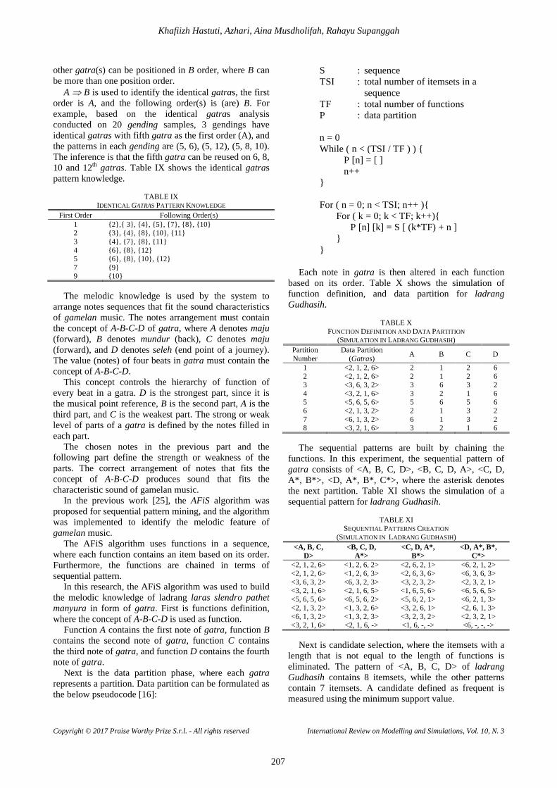
Khafiizh Hastuti, Azhari, Aina Musdholifah, Rahayu Supanggah
Copyright © 2017 Praise Worthy Prize S.r.l. - All rights reserved International Review on Modelling and Simulations, Vol. 10, N. 3
207
other gatra(s) can be positioned in B order, where B can be more than one position order.
A B is used to identify the identical gatras, the first order is A, and the following order(s) is (are) B. For example, based on the identical gatras analysis conducted on 20 gending samples, 3 gendings have identical gatras with fifth gatra as the first order (A), and the patterns in each gending are (5, 6), (5, 12), (5, 8, 10). The inference is that the fifth gatra can be reused on 6, 8, 10 and 12th gatras. Table IX shows the identical gatras pattern knowledge.
TABLE IX
IDENTICAL GATRAS PATTERN KNOWLEDGE First Order Following Order(s)
1 2, 3, 4, 5, 7, 8, 10 2 3, 4, 8, 10, 11 3 4, 7, 8, 11 4 6, 8, 12 5 6, 8, 10, 12 7 9 9 10
The melodic knowledge is used by the system to
arrange notes sequences that fit the sound characteristics of gamelan music. The notes arrangement must contain the concept of A-B-C-D of gatra, where A denotes maju (forward), B denotes mundur (back), C denotes maju (forward), and D denotes seleh (end point of a journey). The value (notes) of four beats in gatra must contain the concept of A-B-C-D.
This concept controls the hierarchy of function of every beat in a gatra. D is the strongest part, since it is the musical point reference, B is the second part, A is the third part, and C is the weakest part. The strong or weak level of parts of a gatra is defined by the notes filled in each part.
The chosen notes in the previous part and the following part define the strength or weakness of the parts. The correct arrangement of notes that fits the concept of A-B-C-D produces sound that fits the characteristic sound of gamelan music.
In the previous work [25], the AFiS algorithm was proposed for sequential pattern mining, and the algorithm was implemented to identify the melodic feature of gamelan music.
The AFiS algorithm uses functions in a sequence, where each function contains an item based on its order. Furthermore, the functions are chained in terms of sequential pattern.
In this research, the AFiS algorithm was used to build the melodic knowledge of ladrang laras slendro pathet manyura in form of gatra. First is functions definition, where the concept of A-B-C-D is used as function.
Function A contains the first note of gatra, function B contains the second note of gatra, function C contains the third note of gatra, and function D contains the fourth note of gatra.
Next is the data partition phase, where each gatra represents a partition. Data partition can be formulated as the below pseudocode [16]:
Each note in gatra is then altered in each function
based on its order. Table X shows the simulation of function definition, and data partition for ladrang Gudhasih.
TABLE X
FUNCTION DEFINITION AND DATA PARTITION (SIMULATION IN LADRANG GUDHASIH)
Partition Number
Data Partition (Gatras) A B C D
1 <2, 1, 2, 6> 2 1 2 6 2 <2, 1, 2, 6> 2 1 2 6 3 <3, 6, 3, 2> 3 6 3 2 4 <3, 2, 1, 6> 3 2 1 6 5 <5, 6, 5, 6> 5 6 5 6 6 <2, 1, 3, 2> 2 1 3 2 7 <6, 1, 3, 2> 6 1 3 2 8 <3, 2, 1, 6> 3 2 1 6
The sequential patterns are built by chaining the
functions. In this experiment, the sequential pattern of gatra consists of <A, B, C, D>, <B, C, D, A>, <C, D, A*, B*>, <D, A*, B*, C*>, where the asterisk denotes the next partition. Table XI shows the simulation of a sequential pattern for ladrang Gudhasih.
TABLE XI
SEQUENTIAL PATTERNS CREATION (SIMULATION IN LADRANG GUDHASIH)
<A, B, C, D>
<B, C, D, A*>
<C, D, A*, B*>
<D, A*, B*, C*>
<2, 1, 2, 6> <1, 2, 6, 2> <2, 6, 2, 1> <6, 2, 1, 2> <2, 1, 2, 6> <1, 2, 6, 3> <2, 6, 3, 6> <6, 3, 6, 3> <3, 6, 3, 2> <6, 3, 2, 3> <3, 2, 3, 2> <2, 3, 2, 1> <3, 2, 1, 6> <2, 1, 6, 5> <1, 6, 5, 6> <6, 5, 6, 5> <5, 6, 5, 6> <6, 5, 6, 2> <5, 6, 2, 1> <6, 2, 1, 3> <2, 1, 3, 2> <1, 3, 2, 6> <3, 2, 6, 1> <2, 6, 1, 3> <6, 1, 3, 2> <1, 3, 2, 3> <3, 2, 3, 2> <2, 3, 2, 1> <3, 2, 1, 6> <2, 1, 6, -> <1, 6, -, -> <6, -, -, ->
Next is candidate selection, where the itemsets with a
length that is not equal to the length of functions is eliminated. The pattern of <A, B, C, D> of ladrang Gudhasih contains 8 itemsets, while the other patterns contain 7 itemsets. A candidate defined as frequent is measured using the minimum support value.
S : sequence TSI : total number of itemsets in a
sequence TF : total number of functions P : data partition n = 0 While ( n < (TSI / TF ) )
P [n] = [ ] n++
For ( n = 0; n < TSI; n++ )
For ( k = 0; k < TF; k++) P [n] [k] = S [ (k*TF) + n ]

Khafiizh Hastuti, Azhari, Aina Musdholifah, Rahayu Supanggah
Copyright © 2017 Praise Worthy Prize S.r.l. - All rights reserved International Review on Modelling and Simulations, Vol. 10, N. 3
208
The given minimum support is 1, which means that an itemset must have at least 1 transaction to be defined as frequent. By setting 1 as the minimum support value, all candidates are frequent.
The above process of function definition, data partition, sequential pattern creation and support counting are implemented to all gending samples. Furthermore, all itemsets in all gending samples are concatenated based on each pattern. Since the given minimum support value is 1, the weight of an itemset after concatenation is not counted.
The duplicate itemsets in each chain are removed. Table XII shows the result of pattern concatenation of <A, B, C, D>, <B, C, D, A>, <C, D, A*, B*>, <D, A*, B*, C*> for all gending samples.
TABLE XII
RESULTS OF SEQUENTIAL PATTERN CONCATENATION OF ALL GENDING SAMPLES
<A, B, C, D> <1, 2, 1, 6>, <1, 2, 5, 3>, <1, 6, 1, 6>, <1, 6, 2, 3>, <1, 6, 3, 2>, <1, 6, 5, 3>, <2, 1, 2, 6>, <2, 1, 3, 2>, <2, 1, 5, 3>, <2, 1, 6, 5>, <2, 3, 1, 6>, <2, 3, 2, 1>, …, <6, 3, 2, 1>
<B, C, D, A*> <1, 2, 6, 1>, <1, 2, 6, 2>, <1, 2, 6, 3>, <1, 2, 6, 5>, <1, 3, 2, 3>, <1, 3, 2, 5>, <1, 3, 2, 6>, <1, 5, 3, 1>, <1, 5, 3, 2>, <1, 5, 3, 5>, <1, 6, 5, 6>, <2, 1, 6, 2>, …, <6, 5, 6, 3>
<C, D, A*, B*> <1, 6, 2, 1>, <1, 6, 2, 3>, <1, 6, 3, 1>, <1, 6, 3, 2>, <1, 6, 3, 6>, <1, 6, 5, 3>, <1, 6, 5, 6>, <2, 1, 2, 1>, <2, 1, 2, 3>, <2, 1, 2, 6>, <2, 1, 3, 2>, <2, 1, 5, 6>, …, <6, 5, 6, 3>
<D, A*, B*, C*> <1, 2, 1, 2>, <1, 2, 3, 2>, <1, 2, 6, 2>, <1, 2, 6, 5>, <1, 3, 2, 1>, <1, 5, 6, 5>, <2, 1, 6, 1>, <2, 1, 6, 3>, <2, 3, 1, 3>, <2, 3, 1, 5>, <2, 3, 2, 1>, <2, 3, 2, 3>, …, <6, 5, 6, 5>
Next is the prune phase to set the following gatra
based on the previous. Pruning of gatra is set by chaining the functions (sequential patterns) as seen in Fig. 5.
Fig. 5. Pruning by chaining the functions
Table XIII shows an example of gatra pruning by chaining the functions for gatra (1216) and (1253). Function <A, B, C, D> is for the previous gatra, and function <A*, B*, C*, D*> is for the following gatra.
TABLE XIII EXAMPLE OF GATRAS PRUNING
<A, B, C, D>
(Previous)
<B, C, D, A*>
<C, D, A*, B*>
<D, A*, B*, C*>
<A*, B*, C*, D*>
(Following)
<1, 2, 1, 6>
<2, 1, 6, 2> <1, 6, 2, 1> <6, 2, 1, 2> <2, 1, 2, 6> <6, 2, 1, 3> <2, 1, 3, 2> <6, 2, 1, 5> <2, 1, 5, 3>
<1, 6, 2, 3> <6, 2, 3, 1> <2, 3, 1, 6>
<2, 1, 6, 3>
<1, 6, 3, 1> <6, 3, 1, 2> <3, 1, 2, 6>
<1, 6, 3, 2> <6, 3, 2, 1> <3, 2, 1, 6>
<6, 3, 2, 3> <3, 2, 3, 1> <3, 2, 3, 2>
<1, 6, 3, 6> <6, 3, 6, 3> <3, 6, 3, 2>
<2, 1, 6, 5>
<1, 6, 5, 3> <6, 5, 3, 1> <5, 3, 1, 6>
<6, 5, 3, 5> <5, 3, 5, 3> <5, 3, 5, 6>
<1, 6, 5, 6>
<6, 5, 6, 2> <5, 6, 2, 1> <6, 5, 6, 3> <5, 6, 3, 2>
<6, 5, 6, 5> <5, 6, 5, 3> <5, 6, 5, 6>
<1, 2, 5, 3>
<2, 5, 3, 1> <5, 3, 1, 2> <3, 1, 2, 1> <1, 2, 1, 6> <3, 1, 2, 5> <1, 2, 5, 3>
<5, 3, 1, 6> <3, 1, 6, 5> <1, 6, 5, 3>
<2, 5, 3, 2> <5, 3, 2, 1> <3, 2, 1, 2> <2, 1, 2, 6> <3, 2, 1, 3> <2, 1, 3, 2>
<2, 5, 3, 5>
<5, 3, 5, 2> <3, 5, 2, 5> <5, 2, 5, 3>
<5, 3, 5, 3> <3, 5, 3, 2> <5, 3, 2, 1>
<3, 5, 3, 5> <5, 3, 5, 3> <5, 3, 5, 6>
<5, 3, 5, 6> <3, 5, 6, 5> <5, 6, 5, 3> <5, 6, 5, 6>
V. Composition Rules Rules of composition are defined based on basic
knowledge, construction knowledge, and melodic knowledge. Therefore, there are basic rules, construction rules, and melodic rules.
In this research, the type of gending used for automatic gamelan music composition is the ladrang laras slendro pathet manyura. The basic knowledge is used to construct a gending. The system built in this research sets the number of gatras to generate a composition using the knowledge of number of gatras and notes (Table IV), and sets the beats in gatra based on the type of balungan using the basic knowledge (Table II). The generation of composition is controlled by construction and melodic rules. The system randomizes the collection of gatras in a sequential pattern of <A, B, C, D> (Table XII) to create notation sequence of composition. The result of the composition is measured using the weight chaining of notes distribution (Table VII), the number and distribution of identical gatras (Table VIII), and gatras pruning (Table XIII).
VI. Genetic Algorithm for Composition Generation
The genetic algorithm is used to generate composition of ladrang laras slendro pathet manyura. There are three main constraints in composition generation: weight distribution of notes, identical gatras, and melodic features. The objective function is formulated as (x1 + x2
A, (B, C, D)
(B, C, D), A*
(C, D, A*), B*
(D, A*, B*), C*
(A*, B*, C*), D*
Previous gatra
Following gatra
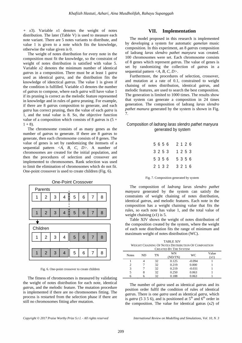
Khafiizh Hastuti, Azhari, Aina Musdholifah, Rahayu Supanggah
Copyright © 2017 Praise Worthy Prize S.r.l. - All rights reserved International Review on Modelling and Simulations, Vol. 10, N. 3
209
+ x3). Variable x1 denotes the weight of notes distribution. The later (Table V) is used to measure each note variant. There are 5 notes variants to distribute, and value 1 is given to a note which fits the knowledge, otherwise the value given is 0.
The weight of notes distribution for every note in the composition must fit the knowledge, so the constraint of weight of notes distribution is satisfied with value 5. Variable x2 denotes the minimum number of identical gatras in a composition. There must be at least 1 gatra used as identical gatra, and the distribution fits the knowledge of idenctical gatras. The value 1 is given if the condition is fulfilled. Variable x3 denotes the number of gatras to compose, where each gatra will have value 1 if its pruning is correct as the melodic feature represented in knowledge and in rules of gatra pruning. For example, if there are 8 gatras composition to generate, and each gatra has correct pruning, then the value of each gatra is 1, and the total value is 8. So, the objective function value of a composition which consists of 8 gatras is (5 + 1 + 8).
The chromosome consists of as many genes as the number of gatras to generate. If there are 8 gatras to generate, then each chromosome consists of 8 genes. The value of genes is set by randomizing the itemsets of a sequential pattern <A, B, C, D>. A number of chromosomes are created for the initial population, and then the procedures of selection and crossover are implemented to chromosomes. Rank selection was used to limit the elimination of chromosomes which do not fit. One-point crossover is used to create children (Fig. 6).
Fig. 6. One-point crossover to create children
The fitness of chromosomes is measured by validating the weight of notes distribution for each note, identical gatras, and the melodic feature. The mutation procedure is implemented if there are no chromosomes fitting. The process is restarted from the selection phase if there are still no chromosomes fitting after mutation.
VII. Implementation The model proposed in this research is implemented
by developing a system for automatic gamelan music composition. In this experiment, an 8 gatras composition of ladrang laras slendro pathet manyura was created. 100 chromosomes were set. Each chromosome consists of 8 genes which represent gatras. The value of genes is set by randomizing the collection of gatras in a sequential pattern <A, B, C, D>.
Furthermore, the procedures of selection, crossover, and mutation at a rate of 0.1, constrained to weight chaining of notes distribution, identical gatras, and melodic features, are used to search the best composition. The generation is limited to 1000 times. The results show that system can generate a composition in 24 times generation. The composition of ladrang laras slendro pathet manura generated by the system is shown in Fig. 7.
Fig. 7. Composition generated by system
The composition of ladrang laras slendro pathet manyura generated by the system can satisfy the constraints of weight chaining of notes distribution, identical gatras, and melodic features. Each note in the composition has a weight chaining value that fits the rules, so each note has value 1, and the total value of weight chaining (x1) is 5.
Table XIV shows the weight of notes distribution of the composition created by the system, where the weight of each note distribution fits the range of minimum and maximum weight of notes distribution (WC).
TABLE XIV
WEIGHT CHAINING OF NOTES DISTRIBUTION OF COMPOSITION CREATED BY THE SYSTEM
Notes ND TN WN (ND/TN) WC Value
(x1) 1 4 32 0.125 -0.094 1 2 7 32 0.219 0.000 1 3 7 32 0.219 -0.031 1 5 8 32 0.250 0.063 1 6 6 32 0.188 0.063 1 The number of gatra used as identical gatras and its
position order fulfil the condition of rules of identical gatras. There is one gatra used as identical gatra, which is gatra (5 3 5 6), and is positioned at 5th and 6th order in the composition. The value for identical gatras (x2) of
1 2 3 4 5 6 7 8
1 2 3 4 5 6 7 8
1 2 3 4 5 6 7 8
1 2 3 4 5 6 7 8
Parents
Children
One-Point Crossover
Composition of ladrang laras slendro pathet manyura generated by system
5 6 5 6 2 1 2 6 3 2 5 3 1 2 5 3 5 3 5 6 5 3 5 6 2 1 3 2 3 2 1 6

Khafiizh Hastuti, Azhari, Aina Musdholifah, Rahayu Supanggah
Copyright © 2017 Praise Worthy Prize S.r.l. - All rights reserved International Review on Modelling and Simulations, Vol. 10, N. 3
210
this composition is 1 (Table XV).
TABLE XV IDENTICAL GATRAS OF COMPOSITION CREATED BY THE SYSTEM
Components Notes Value (x2)
Number of identical gatras 1 (5 3 5 6) 1
Position order 5st, 6th The gatras pruning in this composition fits the rules of
melodic features. The value of gatras pruning of each gatra is 1, if the following gatra is matches the prune of the previous gatra. The evaluation shows that all gatras in the composition have matching following gatras in their pruning. The composition has 8 gatras, and each gatra has a matching following gatra, therefore the total value (x3) achieved is 8 (Table XVI).
TABLE XVI
GATRAS PRUNING OF COMPOSITION CREATED BY THE SYSTEM
NO Previous Gatra Following Gatra Gatra Prunning Value
1 5 6 5 6 2 1 2 6 True 1 2 2 1 2 6 3 2 5 3 True 1 3 3 2 5 3 1 2 5 3 True 1 4 1 2 5 3 5 3 5 6 True 1 5 5 3 5 6 5 3 5 6 True 1 6 5 3 5 6 2 1 3 2 True 1 7 2 1 3 2 3 2 1 6 True 1 8 3 2 1 6 5 6 5 6 True 1
The objective function which must be fulfilled is (x1
+ x2 + x3), where x1 = 5, x2 = 1, and x3 = 8. The implementation of the genetic algorithm can satisfy the constraints to generate an 8 gatras composition of ladrang laras slendro pathet manyura.
VIII. Evaluation The evaluation is conducted to measure the quality of
sound of the composition of ladrang laras slendro pathet manyura created by the system. A framework of evaluation of algorithmic composition proposed by [28] was used. The evaluation is conducted based on Turing test which involves human experts to recognize the composition created by the system.
In this evaluation, a collection of ladrang laras slendro pathet manyura was used, which consists of 5 gendings composed by humans: Ghudasih, Lomanis, Sri Katon, Thinik, and Wilujeng Alus, and add a composition generated by the system to the collection.
The gendings in collection are arranged randomly as seen in Table XVII. Further, six gamelan experts with a background of leaders of gamelan studio, gamelan practitioners, and lecturers, are asked to recognize a composition created by the system in the collection, to assess the difficulty level in recognizing a composition created by system, and to define the pathet of each composition.
The evaluation results show that two out of six gamelan experts can correctly recognize a composition created by the system.
TABLE XVII COLLECTION OF GENDINGS EVALUATED BY GAMELAN EXPERTS
ID Gending Title Notes G1 Gudhasih 2 1 2 6 2 1 2 6
3 6 3 2 3 2 1 6 5 6 5 6 2 1 3 2 6 1 3 2 3 2 1 6
G2 Lomanis 1 6 3 2 3 1 3 2 3 2 1 6 3 2 1 6 5 6 5 6 2 1 5 3 2 1 2 6 3 2 1 6
G3 Sri Katon 2 1 2 6 2 1 2 6 2 1 2 6 3 6 3 2 5 6 5 3 1 6 5 3 2 1 2 6 2 1 2 6
G4 System 5 6 5 6 2 1 2 6 3 2 5 3 1 2 5 3 5 3 5 6 5 3 5 6 2 1 3 2 3 2 1 6
G5 Thinik 2 1 2 6 2 1 2 6 1 6 3 2 3 2 1 6 5 3 5 6 5 3 5 6 2 1 3 2 3 2 1 6
G6 Wilujeng Alus 2 3 1 6 3 6 3 2 5 3 1 6 2 3 1 6 5 6 5 6 2 1 3 2 5 6 5 6 3 2 1 6
The evaluation continues by asking the experts to
evaluate the difficulty level in recognizing a composition created by a human or the system. The value in scale of 1-5 is given to evaluate the difficulty level, where value 1 indicates very easy and value 5 indicates very difficult. All the experts give value 5 in recognizing a composition created by humans or generated by the system. To define the pathet of each gending, all the experts state that all the gendings in the collection have manyura as type of pathet.
Table XVIII shows the evaluation result, with item *G4 indicating the composition generated by system. Column I in the table is about recognizing a composition created by the system, with symbol denoting a correct answer, and x denoting a wrong answer; Column II is about the difficulty level with value in scale of 1-5, where value 5 indicates very difficult; Column III is about the type of pathet of each gending in collection, where 5 composition created by humans have manyura as their type of pathet, and a composition generated by systems is aimed at pathet manyura.
TABLE XVIII
RESULT OF THE EVALUATION Experts I II III
1 *G4 5 All Manyura 2 G3 x 5 All Manyura 3 *G4 5 All Manyura 4 G6 x 5 All Manyura 5 G6 x 5 All Manyura 6 G2 x 5 All Manyura
IX. Conclusion and Future Works The evaluation by gamelan experts results show that
the composition generated by the system is very difficult to be differentiated from the composition created by humans. 4 out of 6 gamelan experts failed to recognize a

Khafiizh Hastuti, Azhari, Aina Musdholifah, Rahayu Supanggah
Copyright © 2017 Praise Worthy Prize S.r.l. - All rights reserved International Review on Modelling and Simulations, Vol. 10, N. 3
211
composition created by the system. Expert 1 and 3 could recognize the composition generated by system, but they agreed that it was very difficult to recognize it, as well as other experts. All experts stated that all the evaluated gending have pathet manyura. This proves that the system can generate a composition with a specific pathet. The model of automatic gamelan music composition proposed in this research is effective, but the element of rasa which can be translated as sensation or inner mining or ability to express or perceive feelings [29], is still not accommodated in this model. The AFiS algorithm can only be used for balungan mlaku and balungan nibani. On the other hand, it needs more types of balungan to explore elements of rasa. In the future works, the AFiS algorithm can be revised to accommodate more types of balungan in analyzing the notes sequence pattern of gamelan music, or the model proposed in this research can be improved by adding elements of ricikan garap, or conducting a classification which includes element of rasa for data training.
References [1] D. Trueman, Why a Laptop Orchestra, Cambridge Journal
Volume 12, 2007. [2] S. Keith, Bridging The Gap: Thoughts On Computer Music And
Contemporary (Popular) Electronic Music, Proceedings of the 2010 Australasian Computer Music Conference, 2010.
[3] J.D. Fernandez, F. Vico, AI Methods in Algorithmic Composition: A Comprehensive Survey, Journal of Artificial Intelligence Research 48, 2013.
[4] E.R. Miranda, Composing Music with Computer, (Focal Press, 2004).
[5] L.A. Hiller, Jr., L.M. Isaacson, Experimental Music: Composition with an Electronic Computer, (McGraw-Hill Book Company, Inc, 1959).
[6] I. Xenakis, Formalized Music: Thought and Mathematics in Composition, (Pendragon Press, 1992).
[7] G. Nierhaus, Algorithmic Composition: Paradigms of Automated Music Generation, (Springer Wien, 2009).
[8] K. Essl, Algorithmic Composition, Cambridge Companion to Electronic Music, ed. by N. Collins and J. d'Escrivan, (Cambridge University Press, 2007).
[9] S. Hastanto, Konsep Pathet Dalam Karawitan Jawa, (ISI Press, 2009)
[10] H. Kridalaksana, F.X. Rahyono, D. Puspitorini, S. Widodo, Darmoko, Wiwara: Pengantar Bahasa dan Kebudayaan Jawa, (Gramedia Pustaka Umum, 2001).
[11] R. Supanggah, Bothekan Karawitan I, (Masyarakat Seni Pertunjukan Indonesia, 2002).
[12] M.C. Ricklefs, Sejarah Indonesia Modern 1200-2008, (PT Serambi Ilmu Semesta, 2008).
[13] S. Nakagawa, Musik dan Kosmos: Sebuah Pengantar Etnomusikologi, (Yayasan Obor Indonesia, 2000).
[14] K. Ebcioglu, An Expert System for Chorale Harmonization, AAAI-86 Procedings, 1986.
[15] R.A. McIntyre, Bach in a Box: The Evolution Of Four Part Baroque Harmony Using The Genetic Algorithm, IEEE World Congress on Computational Intelligence, 1994.
[16] J. Becker, A. Becker, A Grammar of the Musical Genre Srepegan, (University of Texas Press, Texas, 1982)
[17] D. W. Hughes, Deep Structure and Surface Structure in Javanese Music: A Grammar of Gendhing Lampah (University of Illinoi Press, Illinois, 1988).
[18] Hastuti, K., Azhari, A., Musdholifah, A., Supanggah, R., Building Melodic Feature Knowledge of Gamelan Music Using Apriori Based on Functions in Sequence (AFiS) Algorithm, (2016)
International Review on Computers and Software (IRECOS), 11 (12), pp. 1127-1137.
[19] J. Gillick, K. Tang, R.M. Keller, Learning Jazz Grammars, Proceedings of the Sound and Music Computing Conference, 2009.
[20] P. Pestana, Lindenmayer systems and the harmony of fractals, Chaotic Modeling and Simulation (CMSIM) 1, 2012.
[21] K. M. Kitani, H. Koike, ImprovGenerator: Online Grammatical Induction For On-The-Fly Improvisation Accompaniment, Proceedings of the International Conference on New Interfaces for Musical Expression, 2010
[22] T.M. Oliwa, Genetic Algorithm and the abc Music Notation Language for Rock Music Composition, Proceedings of the 10th annual conference on Genetic and evolutionary computation, ACM, 2008
[23] D. Matic, A Genetic Algorithm for Composing Music, Yugoslav Journal of Operations Research, Volume 20, 2010.
[24] N. Fortier, M.V. Dyne, A Genetic Algorithm Approach to Improve Automated Music Composition, International Journal of Computers, Issue 4, Volume 5, 2011.
[25] K. Hastuti, A Method for Automatic Gamelan Music Composition, International Journal of Advances in Intelligent Informatics Vol 2, No 1, 2016.
[26] Sumarsam, Introduction To Javanese Gamelan, (Spiral-bound, 1988)
[27] R. Supanggah, Bothekan Karawitan II: Garap, (ISI Press, 2007). [28] M. Pearce, G. Wiggins, Towards a framework for the evaluation
of machine compositions, Proceedings of the AISB 2001, 2001. [29] M. Benamou, Rasa: Affect and Intuition in Javanese Musical
Aesthetics, Oxford University Press, 2010.
Authors’ information 1Faculty of Mathematics and Natural Science, Universitas Gadjah Mada, Yogyakarta, Indonesia. E-mails: [email protected] [email protected] 2Faculty of Computer Science, Universitas Dian Nuswantoro, Semarang, Indonesia. E-mail: [email protected] 3Faculty of Performing Arts, Institut Seni Indonesa, Surakarta, Indonesia. E-mail: [email protected]
Khafiizh Hastuti received her M.Kom degree in 2012 from informatics Engineering Department of Universitas Dian Nuswantoro. Her research interests are artificial intelligence, data mining, and software engineering.
Azhari Department of Computer Science and Electronics Universitas Gadjah Mada. Undergraduate Statistics Universitas Gadjah Mada, Master of Software Engineering Institut Teknologi Bandung, Doctor of Computer Science Universitas Gadjah Mada. Research interests are Intelligent agent, software engineering, project management.
Aina Musdholifah Department of Computer Science and Electronics Universitas Gadjah Mada.Undergraduate and master of computer science Universitas Gadjah Mada, Ph.D Computer Science Universiti Teknologi Malaysia (UTM). Research interests are genetic algorithm, fuzzy system.

Khafiizh Hastuti, Azhari, Aina Musdholifah, Rahayu Supanggah
Copyright © 2017 Praise Worthy Prize S.r.l. - All rights reserved International Review on Modelling and Simulations, Vol. 10, N. 3
212
Rahayu Supanggah Professor of Ethnomusicology and Music Composition, at ISI Surakarta. Doctorat de 3ème cycle Etnomusicologie, diplomé 1985. Maestro of karawitan composition.

1974-983X(201706)10:3;1-Q