International Transmission of Monetary Shocks:Mundell-Fleming vs Obstfeld-Rogo¤¤

Carlos Borondoy

Universidad de Valladolid

February 2001

Abstract

This paper compares two models of the international transmissionof monetary shocks: the traditional Mundell-Fleming-Dornbusch (MFD)model and the intertemporal and microfounded Obstfeld-Rogo¤ (OR)model. The di¤erences and similarities between them are pointed outand the extensions of the OR model are reviewed.

JEL classi…cation: E32, E52, F41Keywords: International transmission, Monetary policy

1 IntroductionKeynesian macroeconomists have devoted considerable e¤ort to deepening themicrofoundations of aggregate supply behavior as a result of the challenge posedby rational expectations to the standard AD-AS framework of the sixties. Inparticular, the aim has been to establish …rmly the empirical result of short-run nonneutrality of money. It was recognized that the missing part of themodel was the explicit imperfections in the markets, and to include them it

¤This research was carried out while I was visiting the University of Oxford. I thankthe Department of Economics for its hospitality. I also thank Oscar Bajo for his manycomments that greatly improved the original version. The usual disclaimer applies.

yFacultad de Economia. Avda. Valle Esgueva 6. 47011 Valladolid. Fax: +34 983 423299.Email: borondo@eco.uva.es

1

was necessary to develop carefully the behavior of rational agents under thoseimperfections. The approach was to develop small, partial equilibrium models,highlighting the implications of the imperfections. On the other hand, Classicaleconomists continued to develop more and more sophisticated dynamic generalequilibrium models, completely speci…ed from microeconomic assumptions butwithout any imperfection. The current situation, as stated by Blanchard (2000),is one in which both research strategies converge in dynamic general equilibriummodels (the Classical methodology) where di¤erent imperfections are systemat-ically included and their e¤ects explored (the Keynesian approach). Accordingto Blanchard, imperfections are going to play a central role in macroeconomicsbecause: (i) “they lead to very di¤erent e¢ciency and welfare characteristics ofthe equilibrium”, thus a¤ecting the role of policy; (ii) they change the propaga-tion mechanisms of shocks; and (iii) they provide new sources of shocks.The Mundell-Fleming (MF) model was based in the IS-LM model, and as

such inherited the criticisms of that framework, collected recently by McCallumand Nelson (1999). A natural extension of the MF model was to incorporatethe supply side to become a medium run model with rational expectations.This was done by Dornbusch (1976) and the resulting model is known as theMundell-Fleming-Dornbusch (MFD) model. A step forward was to address themicrofoundations of the supply side and to make the model truly dynamic withthe implications of intertemporal utility maximization. This is the contributionof Obstfeld and Rogo¤ (1995). Though they do not include a treatment of theadjustment process of prices, they prepare the model for this task by changingthe framework to a monopolistic competition market. In the general accountof the macroeconomic developments of Blanchard, the Obstfeld-Rogo¤ (OR)model can be considered the successor of the MFD model. There is now ahuge literature extending the OR model, usually referred to as the New OpenEconomy Macroeconomics, and a comprehensive survey is available in Lane(2001).The purpose of this paper is to detail in which ways the explicit consideration

of intertemporal maximization can change the familiar results of the MFDmodelin the two-country version and in the presence of monetary shocks. We o¤er adetailed road map at the cost of narrowing the scope. Being more speci…c makesit possible to highlight the crucial parameters, mechanisms, contributions andapplications.

The structure of the paper is as follows. The next section explains the mainconclusions of a dynamic version of the MFD model based on Taylor’s over-lapping contracts model. The one time, permanent increase of the monetaryaggregate increases Home output and produces an uncertain e¤ect on Foreignoutput (in the original MF case, without expectations, it de…nitely decreases).For international transmission the trade channel is the most important, con-sisting of the expenditure switching e¤ect from Foreign to Home goods (due tothe rise of the relative price of Foreign goods) and the income e¤ect (the in-crease in Home income increases the demand of Foreign products). We explorea second version of the MFD model with Consumer Price Indexes (CPIs), whichadd a new liquidity channel: the depreciation of Home currency reduces ForeignCPI and increases its real balances. With this additional channel the e¤ect onForeign output can be positive.Section three describes the OR model. The intertemporal behaviour of con-

2

sumers is re‡ected in the consumption Euler equation, implying that the real in-terest rate and the expected future consumption are the determinants of currentconsumption. Purchasing Power Parity (PPP) prevails at all times, implyingreal interest rate parity between both countries, and due to the Euler equationboth consumptions follow the same path. As a result, the …nancial channelof transmission becomes more important: when the Home country increasesits monetary aggregate, the real interest rate decreases and the same happensin the other country, resulting in both consumptions increasing. At the sametime, the trade channel is also working, and the expenditure switching e¤ectwill prevail, making Home output increase and the Foreign one decrease. Anew interesting e¤ect is that the Home country can develop a current accountsurplus that will permanently increase its assets against the Foreign country,and this will provide the basis for a long term real e¤ect of the monetary shock.In this section we show that, surprisingly, the welfare e¤ects are positive andof the same amount in both countries, and this is probably the most importantcontribution of this general equilibrium approach.Section four extends the OR model in new directions. The …rst one is the

case with di¤erent cross-country and within-country elasticities of substitutionbetween goods, a case put forward by Tille(2000). The section also considerstwo ways of avoiding the PPP. The …rst is to consider nontraded goods, and thesecond is home bias in preferences. A third direction is the pricing to market(PTM) and local currency pricing (LCP) behaviours of …rms. A …nal directionof research is to include monetary policy rules, both in the Taylor and optimalrules types.Finally, the last section o¤ers the conclusions.

2 The two-countryMundell-Fleming-Dornbuschmodel

Since the Robert Mundell (1962, 1963, 1968) and Marcus Fleming (1962) con-tributions, the Mundell-Fleming model has been the most important analyticalframework to study the international transmission of monetary shocks1. Theoriginal version was based on the IS-LM model, with no dynamics and no ex-pectations. A major improvement was the contribution of Dornbusch (1976)adding rational expectations on the exchange rate movements and a sluggishadjustment of prices. The resulting MFD model is the benchmark with whichto compare the Obstfeld-Rogo¤ model in the next sections.The two-country model, which we label MFD1, assumes symmetry between

countries and contains the following equations:2

1Plus of course for other purposes, but we are focussing here only on this topic.2A few references with very close versions of the model are McCallum (1996), Krugman

(1995), Turnovsky (1986).

3

MFD1 Model

yt = ¡b1rt ¡ b2qt + b3y¤t (1)

y¤t = ¡b1r¤t + b2qt + b3yt (2)

rt = it ¡¡Etp

ht+1 ¡ pht

¢(3)

r¤t = i¤t ¡ (Etp¤ft+1 ¡ p¤ft ) (4)

qt = pht ¡ st ¡ p¤ft (5)

mt ¡ pht = c1yt ¡ c2it (6)

m¤t ¡ p¤ft = c1y

¤t ¡ c2i¤t (7)

it = i¤t +Etst+1 ¡ st (8)

phat =1

2Et¡1

¡pht + °yt + p

ht+1 + °yt+1

¢(9)

p¤fat =1

2Et¡1

³p¤ft + °y¤t + p

¤ft+1 + °y

¤t+1

´(10)

pht =1

2

¡phat + phat¡1

¢(11)

p¤ft =1

2

³p¤fat + p¤fat¡1

´(12)

Table 1 lists the variables used in this and the following sections. All of themare log deviations from trend except the interest rates.

Table 1. Variables in MFD and OR modelsy output (log deviation)c consumption (log deviation)i nominal interest rate (deviation)r real interest rate (deviation)ph; p¤f domestic price index (log deviation)pha; p¤fa price …xed by …rms (log deviation)p consumer price index (log deviation)s nominal exchange rate (log deviation)q terms of trade (q = ph ¡ s¡ p¤f )e real exchange rate (e = s+ p¤ ¡ p)m monetary aggregate (log deviation)

Equations (1) and (2) are the IS schedules and the LM schedules are theexpressions (6) and (7). Equation (8) is the Uncovered Interest Parity (UIP).We are assuming perfect capital mobility between both countries. These eightequations could be solved for the eight variables (y; y¤; i; i¤; s; r; r¤; q) under theassumption that prices are constant, then the model is a short run, …xed pricemodel (if we assume static expectations, we have the Mundell-Fleming model).A second possibility is to solve the equations for (ph; p¤f ; i; i¤; s; r¤; r; q) underthe alternative assumption that prices are perfectly ‡exible and outputs areequal to their natural exogenous levels (y = y¤ = 0). Finally, we can add to the…rst …ve equations some kind of price adjustment mechanism. The Dornbusch(1976) type of adjustment is to assume that prices increase when output is abovethe trend: ¢pt+1 = ¼yt: Our choice is to use the somewhat more elaboratemechanism designed by Taylor (1980): a two-period, staggered-prices structure.Equations (9) and (10) determine the price …xed by …rms for periods t and t+1

4

based on the information available in t-1. The price index in t is the average ofthe existing prices in that period.The only stochastic shocks in the model come from the monetary aggregates,

which we assume follow the general processes:

mt = mt¡1 + utm¤t = m¤

t¡1 + u¤t

ut = ½ut¡1 + "tu¤t = ½u¤t¡1 + "

¤t (13)

where ½ is the autocorrelation of the shocks u; u¤ while "; "¤ are the monetaryinnovations of period t, which we assume are white noise. The coe¢cients ofthe model are taken from Taylor (1993a) and shown in Table 2. Although theyare not estimated values, we can think of them as being reasonable values forthe simulation exercises.

Table 2. Baseline parameter values for the MFD modelb1 = 1:2 b2 = 0:1 b3 = 0:1 c1 = 1 c2 = 4 ° = 1

The experiment is a permanent one-time shock to the home monetary ag-gregate without spillover (½ = 0): The results of the simulation are presented inFigure 1. Home output increases temporarily (in period 4 it is almost back tothe initial steady state level) due to the depreciation of the real exchange rateand the fall of the real interest rate. The Foreign output is almost una¤ectedsince the Foreign real interest rate is una¤ected as well, and the negative e¤ectof the real exchange rate and the positive of the increase in Home output almostcancel each other out. There are two channels through which the Home mon-etary expansion could a¤ect Foreign output: trade and the …nancial market.The trade channel is related to the expenditure switching e¤ect caused by thedepreciation of Home real exchange rate, captured by parameter b2, and to theincome e¤ect due to the increase of Home output that will increase the demandfor Foreign products at the same relative price (b3). The …nancial market chan-nel is related to the UIP that links both nominal interest rates. When the Homecountry increases its monetary aggregate its nominal interest decreases, and thenegative di¤erential is absorbed by the expected rate of depreciation, which willbe negative, implying an expected appreciation, hence the nominal exchangerate overshoots the new long run value. This isolates the Foreign nominal inter-est rate. Without expectations on the exchange rate the Foreign interest ratewould have to fall to match the Home rate, in order to balance the internationalmovements of capital.An interesting addition is the consumer price index (CPI) in which foreign

products represent a fraction of the consumption basket so that movementsof the exchange rate imply changes in the price index and in the real moneybalances. This feature adds a new liquidity channel. The new model is labelledMFD2 below:

5

MFD2 Model

yt = ¡b1rt ¡ b2qt + b3y¤t (14)

y¤t = ¡b1r¤t + b2qt + b3yt (15)

rt = it ¡ (Etpt+1 ¡ pt) (16)

r¤t = i¤t ¡ (Etp¤t+1 ¡ p¤t ) (17)

qt = pht ¡ st ¡ p¤ft (18)

pt = ®pht + (1¡ ®)(st + p¤ft ) (19)

p¤t = ®p¤ft + (1¡ ®)(pht ¡ st) (20)

mt ¡ pt = c1yt ¡ c2it (21)

m¤t ¡ p¤t = c1y

¤t ¡ c2i¤t (22)

it = i¤t +Etst+1 ¡ st (23)

phat =1

2Et¡1 (pt + °yt + pt+1 + °yt+1) (24)

p¤fat =1

2Et¡1

¡p¤t + °y

¤t + p

¤t+1 + °y

¤t+1

¢(25)

pht =1

2

¡phat + phat¡1

¢(26)

p¤ft =1

2

³p¤fat + p¤fat¡1

´(27)

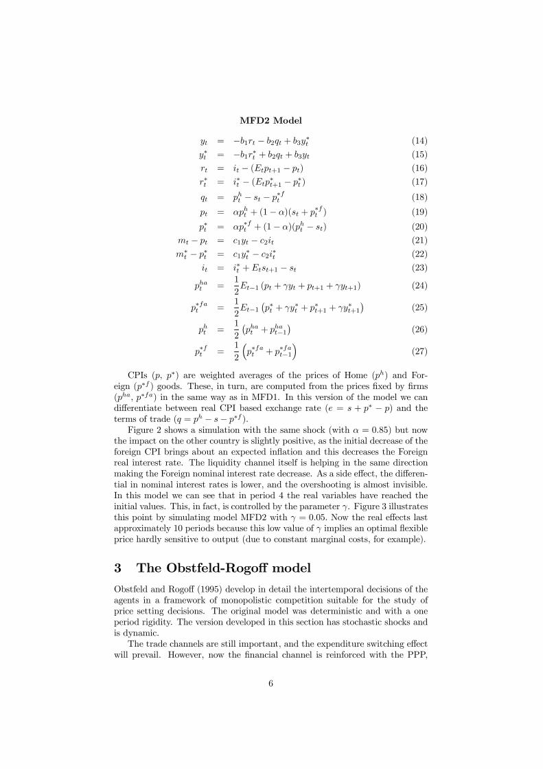
CPIs (p; p¤) are weighted averages of the prices of Home (ph) and For-eign (p¤f ) goods. These, in turn, are computed from the prices …xed by …rms(pha; p¤fa) in the same way as in MFD1. In this version of the model we candi¤erentiate between real CPI based exchange rate (e = s + p¤ ¡ p) and theterms of trade (q = ph ¡ s¡ p¤f ).Figure 2 shows a simulation with the same shock (with ® = 0:85) but now

the impact on the other country is slightly positive, as the initial decrease of theforeign CPI brings about an expected in‡ation and this decreases the Foreignreal interest rate. The liquidity channel itself is helping in the same directionmaking the Foreign nominal interest rate decrease. As a side e¤ect, the di¤eren-tial in nominal interest rates is lower, and the overshooting is almost invisible.In this model we can see that in period 4 the real variables have reached theinitial values. This, in fact, is controlled by the parameter °. Figure 3 illustratesthis point by simulating model MFD2 with ° = 0:05: Now the real e¤ects lastapproximately 10 periods because this low value of ° implies an optimal ‡exibleprice hardly sensitive to output (due to constant marginal costs, for example).

3 The Obstfeld-Rogo¤ modelObstfeld and Rogo¤ (1995) develop in detail the intertemporal decisions of theagents in a framework of monopolistic competition suitable for the study ofprice setting decisions. The original model was deterministic and with a oneperiod rigidity. The version developed in this section has stochastic shocks andis dynamic.The trade channels are still important, and the expenditure switching e¤ect

will prevail. However, now the …nancial channel is reinforced with the PPP,

6

making the real interest parity to hold at all times. This implies that when theHome authority increases the money supply, thus decreasing the real interestrate, the Foreign real interest rate decreases as well. The decline of the realinterest rate, through the intertemporal allocation of consumption, increasescurrent consumption in both countries. In addition, a new channel appears:an international transfer of wealth. This is due to the current account surplusobtained in the Home country, which entitles Home to more assets against theForeign country, thus supporting a permanent relative increase in per capitaconsumption.Another important result is that there is no overshooting of the nominal

exchange rate, instead it will adjust fully to the new long run level in the …rstperiod. We will see in the following sections di¤erent versions of the model inwhich there can be overshooting.The main result of the model is the welfare e¤ect of the asymmetric mone-

tary policy considered: both countries enjoy an increase in welfare of the sameproportion. This remarkable result is subject to the special characteristics ofthe model, and it will be discussed in the next sections.

3.1 The setup

There is a continuum of individuals, z 2 [0; 1], distributed in two countries:home, with z 2 [0; n], and foreign with z 2 (n; 1]. Each individual is a consumerand a producer, and has the utility function:

Ut =1Xs=t

¯s¡tus(C;M

P; Y (z))

=1Xs=t

¯s¡t½logCs + Â log

µMs

Ps

¶¡ '2Ys(z)

2

¾(28)

where 0 < ¯ < 1; and Â;' > 0: Uppercase letters are used for levels. Thede…nition of the consumption index C is

C =

½Z 1

0

[C(z)]µ¡1µ dz

¾ µµ¡1

; µ > 1

where µ is the elasticity of substitution between goods, assumed greater than oneto ensure that marginal revenue of producers is positive (see demand equationbelow). The cost minimizing price index is:

P =

½Z 1

0

[P (z)]1¡µ dz¾ 1

1¡µ

where P (z) is the domestic price of a good z:We allow the Law of One Price to hold so that, if S denotes the nominal

exchange rate then, for any product z, P (z) = SP¤(z): This implies, by thede…nition of the price index, that the PPP holds:

P = SP ¤

7

The individual demands of home and foreign consumers are functions of therelative prices, the elasticity of substitution and the consumption indexes:

C(z) =

·P (z)

P

¸¡µC ; z 2 [0; n]

C¤(z) =

·P ¤(z)P ¤

¸¡µC¤ ; z 2 (n; 1]

where we have already included the assumption of within country symmetry,so that C; C¤ are the aggregate per capita consumptions of each country. Thesymmetry also implies that within a country all prices are equal, so we canwrite:

P (z) = Ph; z 2 [0; n]P ¤(z) = P¤f ; z 2 (n; 1]

With the above individual demands we can compute the global demand foran individual good z:

Y (z) =

·Ph

P

¸¡µCw; z 2 [0; n] (29)

Y ¤(z) =

·P¤f

P ¤

¸¡µCw; z 2 (n; 1]

where Cw is the world per capita consumption, de…ned as:

Cw ´ nC + (1¡ n)C¤

The individual home resident period budget constraint is:

PtBt +Mt + PtCt = (30)

Pt(1 +Rt¡1)Bt¡1 +Mt¡1 + Pt(z)Yt(z) + PtTt

where Bt¡1 is the (end of period) holdings of the unique real bond traded be-tween both countries, Rt¡1is the real interest rate,Mt¡1is the stock of domesticmoney, Yt(z) is the individual production and Tt is the net transfer from gov-ernment. The government maintains in every period a balanced budget (in percapita terms):

Tt =Mt ¡Mt¡1

Pt

The nominal interest rate It is de…ned in the Fisher relationship:

1 + It =EtPt+1Pt

(1 +Rt)

where Et is the expectation operator. The UIP:

1 + It =EtSt+1St

(1 + I¤t )

8

and the PPP imply that the real interest parity also holds:

Rt = R¤t

The behavior of the representative agent is obtained by maximizing theutility function U in (28) subject to the global demand for his product in (29)and the budget constraint in (30). The …rst order conditions (FOCs) faced bythe home representative agent are (similar conditions hold for the foreign agent):

EtCt+1 = ¯(1 +Rt)Ct (31)

Mt

Pt=

µ1

ÂCt¡ ¯ Pt

ÂEt(Pt+1Ct+1)

¶¡1= ÂCt

µ1 + ItIt

¶(32)

Pt(z)µ+1 = P µ+1t

µµ'

µ ¡ 1¶CtC

wt (33)

The …rst is the consumption Euler condition and implies that current consump-tion depends on real interest rate and expected future consumption. The secondcondition determines the demand for money as a positive function of consump-tion (instead of income) and negative of nominal interest rate. The third condi-tion says that the optimal price for producer z is an increasing function of theprice index, of his consumption and of global demand.The equilibrium condition in the global market for the only bond is:

nBt + (1¡ n)B¤t = 0 (34)

This condition and the national budget constraints imply:

Cwt = nPht YtPt

+ (1¡ n)P¤ft Y

¤t

P ¤t= Y wt

where Y wt is the world aggregate per capita real income. This is the world’sresource constraint in per capita terms.To solve the model we consider a symmetric steady state (denoted with a

bar over a variable) where B = B¤= 0. In the steady state:

I = R =1¡ ¯¯

C = C¤= Y = Y

¤=

µµ ¡ 1µ'

¶1=2P = P

h= ÂR

M

C

P¤= P

¤f= ÂR

M¤

C

S =P

P¤ =

M

M¤

Real interest rate is determined by the subjective discount rate ¯: Per capitaconsumption is equal in both countries and …xed by the supply side parameters.Price levels re‡ect the money supply in each country, and the nominal exchangerate the PPP. If prices are perfectly ‡exible monetary shocks are neutral in thelong run, the only steady state e¤ects would be on the nominal variables.

9

3.2 Linearized version of the model

The model is solved by linearizing the equations around the initial steady state(see appendix for the details). Lowercase letters are log deviations of the upper-case variables from their steady state values (except for the nominal and realinterest rates which are level deviations from their steady state values).

OR Model

bt = (1 +R)bt¡1 + pht + yt ¡ pt ¡ ct (35)

¡ n

1¡ nbt = ¡ n

1¡ n(1 +R)bt¡1 + p¤ft + y¤t ¡ p¤t ¡ c¤t (36)

qt = pht ¡ st ¡ p¤ft (37)

yt ¡ y¤t = ¡µqt (38)

(1 + µ)pht = (1 + µ)pt + ct + [nct + (1¡ n)c¤t ] (39)

(1 + µ)p¤ft = (1 + µ)p¤t + c¤t + [nct + (1¡ n)c¤t ] (40)

ct ¡ c¤t = Et[ct+1 ¡ c¤t+1] (41)

mt ¡ pt = ct ¡ 1

R(Etct+1 ¡ ct)¡ 1

R(Etpt+1 ¡ pt) (42)

m¤t ¡ p¤t = c¤t ¡

1

R(Etc

¤t+1 ¡ c¤t )¡

1

R(Etp

¤t+1 ¡ p¤t ) (43)

pt = npht + (1¡ n)hst + p

¤ft

i(44)

p¤t = n£pht ¡ st

¤+ (1¡ n)p¤ft (45)

mt = mt¡1 + "t (46)

m¤t = m¤

t¡1 + "¤t (47)

The …rst two equations are the expressions for the current account, includingthat nbt+(1¡n)b¤t = 0 in the second equation, where b is the net foreign assetposition. Together they imply the global resource constraint cw = yw, wherecwt = nct + (1¡ n)ct and ywt = n(pht + yt ¡ pt) + (1¡ n)(p¤ft + y¤t ¡ p¤t ).Equation (37) de…nes the terms of trade. Note that in this model the PPP

prevails, so that the real exchange rate is constant, but the terms of trade is not.Equation (38) comes from substracting the global demands faced by producersof both countries. The parameter µ is the critical one in this model, as it controlsthe magnitude of the expenditure switching e¤ect after a change in the terms oftrade. Equations (39) and (40) are the optimal prices for the monopolists, andimply that, ceteris paribus, an increase in the CPI will be matched with an equalincrease in the monopolist price, that an increase in world consumption (a shiftin demand) will increase the price and that an increase in home consumptionwill increase the marginal disutility of supplying an additional unit, and thusthe monopolist will increase the price. Equation (41) follows from substractingthe consumption Euler equations in each country, taking into account that thereal interest rate will be the same in each country. Equations (42) and (43)are the money market equilibrium conditions. Finally, (44) and (45) are theloglinearized versions of the CPIs.The 11 equations (35)-(45) determine the 11 variables: y; y¤; c; c¤; p; p¤; ph;

p¤f ; q; s; b given the stochastic processes for m; m¤ in (46)-(47). The shocks tothe monetary aggregates are permanent:

10

In this model the neutrality of money holds in the long and short run. Onlyprices (including the exchange rate) will increase if the money stock increases.

3.3 One period rigid prices

As a …rst step towards a dynamic model with price stickiness, we must constructa one period …xed price version. Henceforth we have to distinguish between theoptimal prices given in (39)-(40), which we will refer to as eph; ep¤f :

epht = pt +1

1 + µct +

1

1 + µcwt (48)

ep¤f = p¤t +1

1 + µc¤t +

1

1 + µcwt

and the actual prices set by …rms: ph; p¤f . The optimal prices do not hold inthe short run, but they do in the long run.To capture that prices are set one period in advance and adjusted every end

of period, we assume the following pricing rules:

pht = Et¡1epht (49)

p¤ft = Et¡1ep¤ftThe solution of the model is explained in the appendix. The exchange rate

is determined combining the conditions for money market equilibrium in bothcountries:

st = (mt ¡m¤t )¡ (ct ¡ c¤t ) (50)

The kind of shock we are analyzing is a permanent one-time increase in theHome monetary aggregate, so that "1 = 1; and "t = 0, for all t > 1: Hence,mt ¡m¤

t = 1 for all t > 0: The Euler equation for consumption implies that

ct ¡ c¤t = c1 ¡ c¤1; for t > 1This implies

s = s1 = 1¡ (c1 ¡ c¤1)where the lowercase letter without time subscript stands for the long run e¤ect,in this case for all t > 1: There is no overshooting in this model because theEuler equation prevents a gradual adjustment in the consumption di¤erential.3

Obstfeld and Rogo¤ (1996, Ch. 9) say that overshooting is not very successfulin practice. In the following sections we will see cases in which overshooting ispossible.The terms of trade follows from the pricing equations and the above equation

for the exchange rate:

qt = ¡"t + (ct ¡ c¤t )¡µ

1 + µ(ct¡1 ¡ c¤t¡1) (51)

3When the consumption elasticity of money demand is not equal to one, the no overshootingresult still holds, as in the original OR(1995) model.

11

The terms of trade will revert to the initial steady state value after a monetaryshock unless there is a permanent di¤erence in per capita consumptions. Usingprevious results:

q1 = ¡1 + (c1 ¡ c¤1) = ¡s1q =

1

1 + µ(c¡ c¤)

the impact (t = 1) is a decline in the terms of trade of the same magnitudebut opposite sign to the increase in the exchange rate. The long run e¤ect isachieved in period 2, with a higher value in the terms of trade if there is arelative increase in consumption in the Home country.The di¤erence in consumptions is in turn:

ct ¡ c¤t = ¼cbbt¡1 + ¼cc(ct¡1 ¡ c¤t¡1) + ¼c""t (52)

¼cb > 0; ¼cc > 0; ¼c" > 0

The impact of the monetary shock is determined by the parameter ¼c" :

¼c" =R(µ2 ¡ 1)

R(1 + µ)µ+ 2µ> 0

This parameter is very small: for our baseline parameter values (µ = 6; n = 0:5;R = 0:01)4 is only 0.028, meaning that 1% increase in money supply createsa gap of 0.028% (of the steady state per capita consumption) between bothcountries. This gap is related to the wealth e¤ect of the current account surplusthat will provide a net foreign asset position permanently higher than the initial:

c¡ c¤ = ¼cb1¡ ¼cc b

However, this e¤ect is very small: in our case ¼cb1¡¼cc = 0:011:

The e¤ect on b comes from the current account surplus of the Home country,which only occurs on the impact (t = 1), because in t = 2 prices adjust to thenew value of m and the new steady state equilibrium is reached where the CAis zero. This implies that b1 = b, and that the initial increase in the net foreignassets is therefore permanent.The last step is to compute the national consumptions and outputs, and for

this we need the world per capita consumption. To compute the e¤ect on worldconsumption we begin by computing the world CPI from the pricing rules:

pwt = npt + (1¡ n)p¤t = Et¡1pwt +2

1 + µEt¡1cwt (53)

This expression implies that there is no impact e¤ect on pwt and that

Etcwt+1 = 0 (54)

so that the expected value of global per capita consumption for the periodafter the shock is the steady state value, because all prices will adjust to the

4We are assuming a quarterly model, so that R = 0:01 is about a 4% annual real interestrate. µ = 6 is the usual value in the literature, taken from markups of around 20% found byRotemberg and Woodford (1992).

12

new monetary conditions at that moment. This in turn implies in the Eulerequation that

cwt = ¡¯rt (55)

Roughly speaking, a decrease of one point in real interest rate will increaseglobal per capita consumption by 1%.To compute cwt we show in the appendix that aggregating the money market

equilibrium conditions and taking into account the pricing rules:

cwt =mwt ¡ pwt = n"t

which shows that the nominal shock will increase global consumption but only inthe period when the innovation takes place. National per capita consumptionscan be obtained as follows:

ct = cwt + (1¡ n)(ct ¡ c¤t ) (56)

c¤t = cwt ¡ n(ct ¡ c¤t )From these expressions it can be concluded that if the wealth e¤ect is small, aswe have seen is the case, both consumptions will increase by practically the sameamount, thus producing the high (almost perfect) correlation between home andforeign consumption.The global resource constraint requires that

cwt = ywt = n(p

h + y ¡ p) + (1¡ n)(p¤f + y¤ ¡ p¤) = ny + (1¡ n)y¤and the national outputs can be computed as:

yt = ywt + (1¡ n)(yt ¡ y¤t ) = n"t ¡ (1¡ n)µqt (57)

y¤t = ywt ¡ n(yt ¡ y¤t ) = n"t + nµqtWe collect all the results in Table 3. While home output will always increase

after a monetary expansion, the e¤ect on foreign output will be negative. Thisimplies a negative correlation of (y; y¤) and also a negative correlation of (y¤;c¤). However, both correlations are positive in the business cycle literature andin the VAR evidence.

Table 3.Results of a one-time permanent increase in the Home monetary aggregate

Short run (t = 1) Long run (t > 1)"t 1 0mt ¡m¤

t 1 1ct ¡ c¤t ¼c² > 0 ¼c² > 0bt

1¡¼cc¼cb

¼c² > 01¡¼cc¼cb

¼c² > 0

st 1¡ ¼c² > 0 1¡ ¼c² > 0qt ¡(1¡ ¼c²) < 0 1

1+µ¼c² > 0

yt ¡ y¤t µ(1¡ ¼c²) > 0 ¡ µ1+µ¼c² < 0

cwt n > 0 0ywt n > 0 0rt = r

¤t ¡ 1

¯n < 0 0

ct n+ (1¡ n)¼c² > 0 (1¡ n)¼c² > 0yt n+ (1¡ n)µ(1¡ ¼c²) > 0 ¡(1¡ n) µ

1+µ¼c² < 0

c¤t n(1¡ ¼c²) > 0 ¡n¼c² < 0y¤t n(1¡ µ)(1¡ ¼c²) < 0 n µ

1+µ¼c² > 0

13

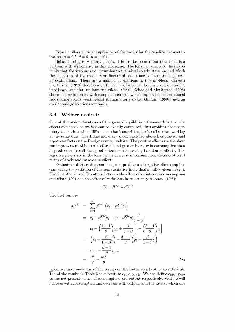
Figure 4 o¤ers a visual impression of the results for the baseline parameter-ization (n = 0:5, µ = 6; R = 0:01).Before turning to welfare analysis, it has to be pointed out that there is a

problem with stationarity in this procedure. The long run e¤ects of the shocksimply that the system is not returning to the initial steady state, around whichthe equations of the model were linearized, and some of them are log-linearapproximations. There are a number of solutions to this problem. Corsettiand Pesenti (1999) develop a particular case in which there is no short run CAimbalance, and thus no long run e¤ect. Chari, Kehoe and McGrattan (1998)choose an environment with complete markets, which implies that internationalrisk sharing avoids wealth redistribution after a shock. Ghironi (1999b) uses anoverlapping generations approach.

3.4 Welfare analysis

One of the main advantages of the general equilibrium framework is that thee¤ects of a shock on welfare can be exactly computed, thus avoiding the uncer-tainty that arises when di¤erent mechanisms with opposite e¤ects are workingat the same time. The Home monetary shock analyzed above has positive andnegative e¤ects on the Foreign country welfare. The positive e¤ects are the shortrun improvement of its terms of trade and greater increase in consumption thanin production (recall that production is an increasing function of e¤ort). Thenegative e¤ects are in the long run: a decrease in consumption, deterioration ofterms of trade and increase in e¤ort.Evaluation of these short and long run, positive and negative e¤ects requires

computing the variation of the representative individual’s utility given in (28).The …rst step is to di¤erentiate between the e¤ect of variations in consumptionand e¤ort (UR) and the e¤ect of variations in real money balances (UM):

dU = dUR + dUM

The …rst term is:

dUR =1Xt=1

¯t¡1³ct ¡ 'Y 2yt

´= c1 ¡ 'Y 2y1 + (c¡ 'Y 2y) ¯

1¡ ¯= c1 ¡

µµ ¡ 1µ

¶y1 +

¯

1¡ ¯·c¡

µµ ¡ 1µ

¶y

¸=

µc1 +

¯

1¡ ¯ c¶¡ µ ¡ 1

µ

µy1 +

¯

1¡ ¯ y¶

= cnpv ¡ µ¡ 1µynpv

=cw1µ=mw1

µ(58)

where we have made use of the results on the initial steady state to substituteY and the results in Table 3 to substitute c1; c; y1; y. We can de…ne cnpv; ynpvas the net present values of consumption and output respectively. Welfare willincrease with consumption and decrease with output, and the rate at which one

14

additional unit of output o¤sets the utility of one additional unit of consumptionis (µ ¡ 1)=µ, the inverse of the margin of the monopolists. In perfect competi-tion this margin is equal to one and an additional unit of output generates adisutility that exactly o¤sets the gain from consuming it, and in that case thereis no welfare improvement with monetary policy. However, with imperfect com-petition, one unit of additional output increases welfare after discounting forthe increase of e¤ort. This is the result put forward by Blanchard and Kiyotaki(1987) in a closed economy.The same procedure for the Foreign country gives

dU¤R =cw1µ=mw1

µ

This is the remarkable result of Obstfeld and Rogo¤ (1995): both countries enjoythe same increase of welfare after the monetary shock. The expenditure switch-ing e¤ect and the permanent change in foreign assets (wealth redistribution)are of second order importance. The reason is that in the initial equilibriummarginal revenue and cost were equal, hence a marginal decrease in the relativeprice of home goods (brought about by the depreciation) will increase revenuesby selling more abroad, but also will increase the e¤ort needed and both in-creases will o¤set each other as long as the shock is marginal. The e¤ect ofthe permanent change in wealth is also of second order importance on utilitybecause it implies a reallocation between consumption and leisure from the ini-tial equilibrium. The important e¤ect is the global increase in demand, as thiswill shift the equilibrium from the initial monopolistic situation towards thecompetitive allocation.The real balance e¤ect on utility does not change the result in the Home

country because real balances increase in all periods, thus increasing Homewelfare even more. In the Foreign country real balances rise in the …rst periodbut fall in the long run (driven by the fall in consumption), but Obstfeld andRogo¤ argue that for plausible parameter values dU¤M > 0:A …nal implication of this welfare analysis is that the beggar-thy-neighbour

conclusion of the standard MF model, based on the expenditure switching e¤ect,can be misleading because in the OR model, we …nd that the foreign countryincreases its welfare in spite of the decrease in output. In fact, the conclusionof Obstfeld and Rogo¤ (1995) can also be misleading, as it is based on certainassumptions which are not particularly plausible. The literature that has fol-lowed their seminal contribution has expanded their framework and has stressedsituations in which the Foreign (or the Home) country can in fact be in a worseposition after the Home monetary expansion.

4 Extension: New Open Economy Macroeco-nomics

This section presents some extensions of the OR model. The …rst one is thecase in which the elasticity of substitution between goods of the same country(the within-country elasticity) is higher than that between national and foreigngoods (the cross-country elasticity). In this case the expenditure switching e¤ectis reduced and the impact on welfare can be quite di¤erent: the loser could bethe country expanding its money and the other country the winner.

15

A second subsection explains di¤erent ways of avoiding the PPA: nontrade-able goods and home bias in preferences. The presence of nontradeable goodsincreases the response of the nominal exchange rate, decreases the expenditureswitching e¤ect and breaks the real interest rate parity. Alternatively, the homebias in preferences can bring about an increase in welfare in the Home countryand a decrease in the other.The third subsection explores a promising direction: the Pricing To Market

(PTM) and Local Currency Pricing (LCP) behavior of …rms. Both featurestend to reduce the pass-through from exchange rates to prices, decreasing theexpenditure switching e¤ect and welfare can increase in the Home country whiledecreasing in the Foreign one.In the last subsection we introduce monetary policy rules, of both the Taylor

and optimal type.

4.1 Cross-country elasticity of substitution

Tille (2000) has added the important distinction between cross-country andwithin-country elasticity of substitution. Rede…ning the consumption index Cthat appears in the utility function (28) allows us to discriminate between homeand foreign goods:

C =

·n

1¸

¡Ch¢¸¡1

¸ + (1¡ n) 1¸ ¡Cf¢¸¡1¸ ¸ ¸¸¡1

, ¸ > 0

where Ch; Cf are the subindexes of the consumption of home produced goodsand foreign produced goods respectively, and ¸ is the elasticity of substitutionbetween them (the cross-country elasticity). The consumption subindexes are:

Ch =

½n¡

1µ

Z n

0

£Ch(z)

¤ µ¡1µ dz

¾ µµ¡1

; µ > 1

Cf =

½(1¡ n)¡ 1

µ

Z 1

n

£Cf (z)

¤ µ¡1µ dz

¾ µµ¡1

where µ is the elasticity of substitution between goods of the same country (thewithin-country elasticity). The cost minimizing price indexes are:

16

Ph =

½1

n

Z n

0

[P (z)]1¡µ dz¾ 1

1¡µ

P f =

½1

1¡ nZ 1

n

£P f (z)

¤1¡µdz

¾ 11¡µ

P =nn¡Ph¢1¡¸

+ (1¡ n) ¡P f¢1¡¸o 11¡¸

P ¤h =

½1

n

Z n

0

[P ¤(z)]1¡µ dz¾ 1

1¡µ

P ¤f =

½1

1¡ nZ 1

n

£P ¤f (z)

¤1¡µdz

¾ 11¡µ

P ¤ =nn¡Ph¢1¡¸

+ (1¡ n) ¡P¤f¢1¡¸o 11¡¸

where P (z) is the domestic price of a home produced good z; P ¤(z) is theforeign price of a home produced good z, P f (z) is the domestic price of aforeign produced good z and P ¤f (z) is the foreign price of a foreign producedgood z.The Law of One Price implies that, for any product z, P (z) = SP ¤(z) and

P f (z) = SP ¤f (z); and by the de…nition of the price indexes: Ph = SP ¤h;P f = SP ¤f and the PPP still holds: P = SP ¤:The steady state is exactly the same as in the standard OR model and

the linearized equations are also the same, except that µ is substituted by ¸.The interesting di¤erent is that if ¸ < µ; as is the most probable case5 , theexpenditure switching e¤ect will be smaller:

yt ¡ yt = ¡¸qt (59)

where we have just substituted µ by ¸: This equation implies that the impactof the Home monetary shock will be smaller in both countries:

y1 = n+ (1¡ n)¸(1¡ ¼c²) > 0y¤1 = n(1¡ ¸)(1¡ ¼c²) < 0

Figure 5 depicts the case with ¸ = 1: The negative impact on Foreign outputwill be smaller the closer ¸ is to one. If there were very low substitution betweenforeign and domestic goods, the depreciation of Home currency will add almostnothing to increase Home output and the other country would enjoy an exactlysimilar expansion (¼c² ¡! 0): However, the lack of substitutability means thatimports will be more expensive, thus reducing national income and consumption.Figure 6 depicts an example with ¸ = 0:01: In this case the Home countryexperiences a de…cit and thus a wealth transfer towards the Foreign country,the terms of trade worsens in the short and in the long run, and consumptionincreases in the short run but severely decreases in the long run. Additionally,

5Chari, Kehoe and McGrattan (1998) report that the elasticity of substitution betweenhome and foreign goods tends to be between 1 and 2, and they choose a value of 1.5 followingBackus, Kehoe and Kydland (1994).

17

the CPI at Home increases more than money, thus reducing real money balancesand reducing welfare. Should we care only of output performance, we would seean increase in the short run in both countries, but this result is clearly misleadingwhen assessing the impact on welfare. This is a clear example of the advantageof using a general equilibrium model to analyze the outcomes of policies. Onthe other hand, a very high substitution implies a huge expenditure switchingfrom foreign to home goods and a better outcome for the Home country.Corsetti-Pesenti (1999) exploit the case ¸ = 1 and, while it is evident from

the above equations that there is an expenditure switching e¤ect, this doesnot produce a change in relative real incomes, so there is no current accountimbalance and no change in the consumption di¤erential. Figure 7 provides agraphical illustration of the results in this case. There is no permanent reale¤ect, since all of the persistent real e¤ects we have seen come from the …rstperiod current account imbalance, and here it is balanced. This result highlightsthe fact that these types of models incorporate a persistence mechanism ofnominal shocks.

4.2 Nontradable goods and home bias

The ful…lment of the Purchasing Power Parity at any time is not an appealingfeature of the model, since the deviations from the PPP are signi…cant andhighly persistent (see the survey by Rogo¤, 1996). Two ways of dealing withthis problem are to include nontradable goods or home bias in preferences. Weturn to these additions in this subsection.

4.2.1 Nontradable goods

Hau (2000) assumes two countries of the same size (n = 12), each one with

a proportion ´ 2 [0; 12 ] of nontradables. There is a continuum of goods z 2[0; 1]: The representative Home agent consumes three types of goods: Homenontradables (z 2 [0; ´]), Home tradables (z 2 [´; 12 ]) and Foreign tradables(z 2 [12 ; 1¡ ´]), and the consumption index is de…ned as:

CI =

·Z 1¡´

0

C(z)µ¡1µ dz

¸ µµ¡1

where µ is the unique elasticity of substitution among the three kinds of goods.The main conclusions are the following. Firstly, from the CPIs we have:

pt ¡ p¤t =1¡ 2´1¡ ´ st

implying that the PPP only holds if there are no nontradables (´ = 0), and thatthe variance of the nominal exchange rate will be greater than the variance ofthe relative prices (as it is found in the IRBC literature). Moreover, de…ningthe degree of openness as:

openness =exportsGDP

=1¡ 2´2(1¡ ´)

it is straightforward to see that the smaller the degree of openness (the biggerthe proportion of nontradables), the greater is the volatility of the exchangerate relative to the CPIs.

18

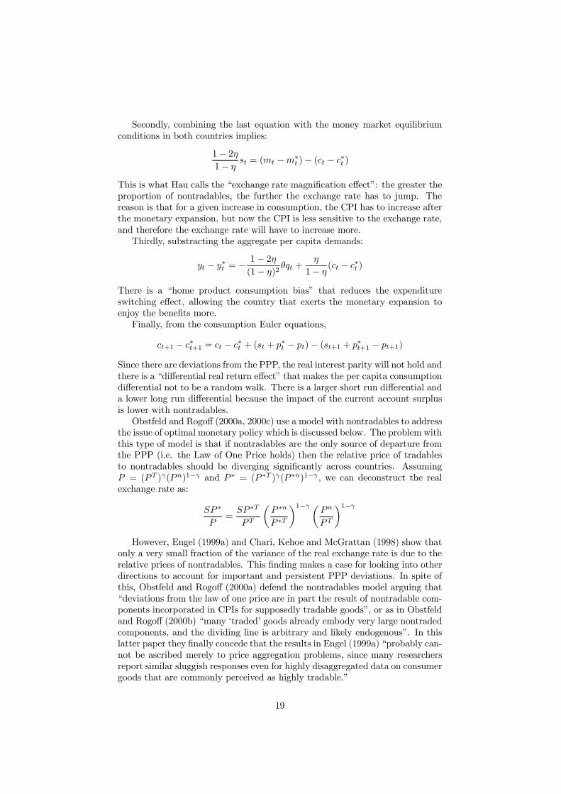
Secondly, combining the last equation with the money market equilibriumconditions in both countries implies:

1¡ 2´1¡ ´ st = (mt ¡m¤

t )¡ (ct ¡ c¤t )

This is what Hau calls the “exchange rate magni…cation e¤ect”: the greater theproportion of nontradables, the further the exchange rate has to jump. Thereason is that for a given increase in consumption, the CPI has to increase afterthe monetary expansion, but now the CPI is less sensitive to the exchange rate,and therefore the exchange rate will have to increase more.Thirdly, substracting the aggregate per capita demands:

yt ¡ y¤t = ¡1¡ 2´(1¡ ´)2 µqt +

´

1¡ ´ (ct ¡ c¤t )

There is a “home product consumption bias” that reduces the expenditureswitching e¤ect, allowing the country that exerts the monetary expansion toenjoy the bene…ts more.Finally, from the consumption Euler equations,

ct+1 ¡ c¤t+1 = ct ¡ c¤t + (st + p¤t ¡ pt)¡ (st+1 + p¤t+1 ¡ pt+1)Since there are deviations from the PPP, the real interest parity will not hold andthere is a “di¤erential real return e¤ect” that makes the per capita consumptiondi¤erential not to be a random walk. There is a larger short run di¤erential anda lower long run di¤erential because the impact of the current account surplusis lower with nontradables.Obstfeld and Rogo¤ (2000a, 2000c) use a model with nontradables to address

the issue of optimal monetary policy which is discussed below. The problem withthis type of model is that if nontradables are the only source of departure fromthe PPP (i.e. the Law of One Price holds) then the relative price of tradablesto nontradables should be diverging signi…cantly across countries. AssumingP = (PT )°(Pn)1¡° and P ¤ = (P ¤T )°(P ¤n)1¡°; we can deconstruct the realexchange rate as:

SP ¤

P=SP ¤T

PT

µP ¤n

P ¤T

¶1¡° µPn

PT

¶1¡°However, Engel (1999a) and Chari, Kehoe and McGrattan (1998) show that

only a very small fraction of the variance of the real exchange rate is due to therelative prices of nontradables. This …nding makes a case for looking into otherdirections to account for important and persistent PPP deviations. In spite ofthis, Obstfeld and Rogo¤ (2000a) defend the nontradables model arguing that“deviations from the law of one price are in part the result of nontradable com-ponents incorporated in CPIs for supposedly tradable goods”, or as in Obstfeldand Rogo¤ (2000b) “many ‘traded’ goods already embody very large nontradedcomponents, and the dividing line is arbitrary and likely endogenous”. In thislatter paper they …nally concede that the results in Engel (1999a) “probably can-not be ascribed merely to price aggregation problems, since many researchersreport similar sluggish responses even for highly disaggregated data on consumergoods that are commonly perceived as highly tradable.”

19

4.2.2 Home bias in preferences

One of the international trade puzzles addressed by Obstfeld and Rogo¤ (2000b)is that consumers seem to have preferences biassed towards the goods producedin their country. They review the evidence and highlight that “the generalconclusion of the literature is that there is a stunning degree of home bias intrade” (p. 13).Warnock (1999) incorporates this feature in the OR model through a pa-

rameter in the utility function. The new de…nition of the consumption indexis

C =

½®

1µ

Z n

0

Ch(z)µ¡1µ dz + (2¡ ®) 1µ

Z 1

n

Cf (z)µ¡1µ dz

¾ µµ¡1

µ > 1; 0 < ® < 2

When ® = 1 there is no home bias and the consumption index reduces to thestandard case of Section 3.1. There is a home bias when ® > 1. The Homeconsumers’ demands for home and foreign goods are:

Ch = ®

µPh

P

¶¡µC

Cf = (2¡ ®)µSP¤f

P

¶¡µC

implying that

Ch

Cf=

®

2¡ ®q¡µ

If the Foreign country has equal bias, then it will be the case that

C¤h

C¤f=2¡ ®®

q¡µ

Therefore, if ® > 1 then

C¤h

C¤f< q¡µ <

Ch

Cf

For any given relative price, the ratio of home to foreign goods consumed ishigher in the Home country.6

The linearized CPIs are:

p = n®ph + (1¡ n)(2¡ ®)(s+ p¤f )p¤ = n(2¡ ®)(ph ¡ s) + (1¡ n)®p¤f

From which we can compute the CPI based real exchange rate:

e = s+ p¤ ¡ p = (®¡ 1)(s+ 2np¤f ¡ 2nph)6Note that both ratios can be greater than one, depending on the relative price.

20

which shows that the PPP is not necessarily ful…lled in this model for ® 6= 1.With home bias (® > 1) the real exchange rate will move proportionally to thenominal exchange rate. The deviation from the PPP will last as long as p¤f ; ph

return to their new steady state level. Moreover, the volatility of the nominalexchange can be several times the volatility of the relative CPIs, one of thestylized facts pointed out by Chari, Kehoe and McGrattan (1998).The expenditure switching e¤ect is now:

yt ¡ y¤t = ¡®(2¡ ®)µq + (®¡ 1)(ct ¡ c¤t )

which collapses to Equation (38) for ® = 1: In the relevant case ® > 1 thee¤ect of the relative price q is smaller as ® tends to 2: the home bias makes therelative price less important.The Home country improves its welfare more than the Foreign one. Indeed,

Warnock computes that the Foreign country’s welfare decreases: the beggar-thy-neighbour e¤ect is more likely as the home bias increases.Ghironi (1999a) builds a model to assess the US-EU interdependence based

in this framework. The only modi…cation is that agents hold a nominal bondinstead of a real bond, thus the movements of the exchange rate have an addi-tional wealth e¤ect. He …nds that for monetary expansions to have a positivee¤ect on consumption a minimum value of µ is required in order to bring aboutan expenditure switching e¤ect strong enough to o¤set the loss from a lowerreal value of assets. He also …nds that the output e¤ect abroad is negative.

4.3 Pricing to Market and Local Currency Pricing

With Pricing To Market (PTM) and Local Currency Pricing (LCP) there is noexpenditure switching e¤ect since there is no immediate pass-through from theexchange rate to prices and thus in both countries output increases. This ne-glects any e¤ect of the exchange rate on the trade ‡ows, and in turn neglects therole of trade as an international transmission channel, a considerable di¤erencefrom the MFD model and with the OR model.The empirical support is double: on the one hand, the failure of the law of

one price, as documented by Engel (1993) and Engel and Rogers (1996, 1998)for example; and on the other hand, the evidence of limited pass-through fromexchange rate movements to prices (see Goldberg and Knetter, 1997, for a reviewof the evidence).Betts and Devereux (2000) develop a model in which a proportion of …rms

can discriminate prices among countries and set prices in the local currency,while the remaining fraction of …rms can not discriminate and set prices inthe producer’s currency. They claim that the PTM behaviour has importantimplications:

Claim 1 PTM limits the pass-through from exchange rate movements to pricemovements.

Claim 2 PTM reduces the expenditure switching e¤ect, thus increasing the cor-relation between Home and Foreign outputs.

Claim 3 PTM and nominal price rigidity increase the volatility of the exchangerate.

21

Claim 4 PTM allows for departures of the PPP, thus breaking the real interestrate parity, and the consumption paths will not be identical, hence the correlationbetween consumptions will be lower.

Claim 5 While Home welfare always increases, Foreign welfare may decrease,and will decrease with full PTM.

These claims are important for the analysis of the international transmissionof shocks, and the last one is particularly relevant for the analysis of policycoordination.

Betts and Devereux (2001) extend the model introducing capital accumula-tion and price dynamics with overlapping contracts à la Calvo and allowing avarying degree both of PTM and of completeness of asset markets. They simu-late the model and …nd the same results as above, which they compare with aVAR model of the US and an agregate of the other G7 countries. The versionof the model with PTM can match the positive comovement of outputs, thedepreciation of the real exchange rate and the increase in nominal interest ratedi¤erential7 after an expansionary monetary shock in the US. In addition, theyshow that the international transmission of monetary shocks is only slightlymodi…ed by the structure of the asset markets.The problems with this PTM approach have been pointed out by Obstfeld

and Rogo¤ (2000a) who “…nd recent models built on the PTM-LCP approachhighly implausible because their assumptions and predictions appear grosslyinconsistent with many other factors”. The most important is the prediction ofa positive correlation between nominal exchange rate and the terms of trade.For di¤erent measures, Obstfeld and Rogo¤ …nd that in most of the countriesthis correlation is negative. However, in a more recent paper, Obstfeld andRogo¤ (2000b) seem to point in that direction to explain the PPP puzzle andthe exchange rate disconnect puzzle: “High volatility and the exchange ratedisconnect therefore both result from a combination of trade costs, monopoly,and pricing to market in local currency. A full model would incorporate thosefactors, while also modeling fully the dynamics of price adjustment throughretail distribution networks, as well as other channels through which exchangerates might a¤ect the real economy” (p. 41).Tille (1999b) avoids the predicted positive correlation between nominal ex-

change rate and the terms of trade by introducing retailers in the model. Firmsof one country sell to retailers of the other country, not directly to consumers.Retailers, in turn, sell to consumers. Firms do not price to market and do notset prices in local currency, but retailers of imported goods can choose either toset the …nal price in local currency (LCP) or in the producer’s currency (Pro-ducer Currency Pricing or PCP). In the …rst case (LCP) all ‡uctuations of theexchange rate are absorbed by the retailer and there is no pass-through, whilein the second case (PCP) the retailer passes all ‡uctuations of the exchange rateto …nal local prices. In this way the global pass-through is controlled by theproportion à of retailers that set prices in local currency. If à = 1 (full LCP)then there is no pass-through at all, as in the Betts and Devereux model with

7This implies overshooting, which is possible in the PTM model when the consumptionelasticity of money demand is smaller than one, and a value of 0.85 is used in the calibration.

22

full PTM. If à = 0 then the pass-through is complete and PPP holds conti-nously. With this addition, even with full LCP, the terms of trade behave inthe same way as in the OR model. The di¤erence is that Home retailers makea loss when there is a devaluation (selling more expensive foreign goods at thesame price), thus the income e¤ect found by Betts and Devereux is still present,but in the opposite direction. Hence the welfare results of a Home monetaryexpansion are reversed: The Home country is worse-o¤ (“beggar-thy-self”) andthe Foreign country is better-o¤. The critical point is the structure of owner-ship of the retailers. In the case just explained all retailers are assumed to beowned by the country where they are. It could be the case however that theretailers selling imported goods are subsidiaries of the other country exporting…rms. In that case the income e¤ect is the opposite: the losses of the Homeretailers are su¤ered by the Foreign owners, and the pro…ts of the Foreign re-tailers are reverted to the Home country. The welfare e¤ect is positive to theHome country and negative to the Foreign country (“beggar-thy-neighbour”).Tille stresses that the welfare result of Betts and Devereux “does not re‡ect theabsence of exchange rate pass-through per se, but instead the allocation of theresulting income e¤ect of exchange rate ‡uctuations” (p. 13). A …nal remark onthis model is that this result is relevant with incomplete international …nancialmarkets, because in the complete market case the ownership of the retailers isirrelevant, and the result of Betts and Devereux holds.Brunnermeier and Grafe (1999) obtain very similar results. Bergin and Feen-

stra (1999) use translog preferences with home bias to motivate the PTM be-haviour of …rms, although their main focus is on persistence of monetary shocks.Chari, Kehoe and McGrattan (1998) also use the PTM behaviour to obtain de-viations from PPP, with similar results to Betts and Devereux (2001).In an interesting application of the Tille (1999) approach to LCP, Devereux,

Engel and Tille (1999) analyse the welfare e¤ects of the euro for Europe and forthe United States. They …nd that the single currency will make it more likelythat the US exporters set prices in euros, in the same way as European exportersare currently pricing in dollars. This change in the price setting behavior willisolate European consumer prices from exchange rate variability, as is the casenow in the US. That insulation increases the expected per capita consumptionin Europe through a relative price stabilizing e¤ect, and therefore the welfare.For the US there is also a positive e¤ect since the increased stability of Europeanprices will increase asset prices and that will increase the value of the portfolioof American investors in Europe.

4.4 Monetary Policy Rules

4.4.1 Taylor type rules

One of the arguments to defend the PTM-LCPmodels is that they predict a pos-itive correlation between Home and Foreign output, as shown by the empiricalevidence8, while the standard OR model predicts a negative output correla-tion. Chari, Kehoe y McGrattan (1998) concede that to achieve this positivecomovement they need to impose a positive correlation in the monetary shocksof both countries: “if money shocks are correlated across countries, the model

8Kim (2000) and Betts and Devereux (2001) carry out a VAR analysis of the e¤ect of theUS monetary policy on the output of the G7 countries and …nd a positive transmission.

23

is broadly consistent with the comovements in output and consumption acrosscountries as seen in the data” (p. 2). Moreover, “increasing the correlation ofthe money shocks increases the cross-country correlation of both output andconsumption” (p. 23) and …nally “the details of the comovements of monetarypolicy across countries is important for the comovements of the aggregates” (p.24). In their …gure 10 they show that without correlation in the money growthrates, the GDP correlation falls to zero. The problem is that they do not o¤erany reason for this positive correlation of monetary policies. Kollmmann (1999)estimates a correlation of 0.20 between monetary innovations in the US and inthe aggregate of the other G7 countries (see Table 1 in his paper), but there isno explanation of why.Borondo (2000) shows that another way to obtain a positive comovement of

outputs is to introduce interest rate rules in both countries that target the CPI.These rules explain the comovement of monetary policies as well. The policyrule for the nominal interest rate (It) is:

It = d0 + d1(logPt ¡ logPT )

where PT is the target consumer price index.9 The price level target becomesthe new steady state value (P = PT ), with the monetary aggregate adjustingendogenously to meet the demand for money. Then, as logPt ¡ logP = pt, itimplies that d0 = R = (1¡ ¯)=¯; and the rule can be …nally written as:

it = It ¡R = d1pt + ut (60)

ut = ½ut¡1 + "t (61)

where u is the monetary shock, assumed to be an AR(1) process with persistence½ and "t is the white noise innovation. With an interest rate rule, monetaryshocks are exogenous stochastic shifts in the feedback rule used by the monetaryauthority, as de…ned by Rotemberg and Woodford (1998, p.4). McCallum andNelson (1999a) also study the impulse responses after a shock to the interestrate rule, interpreted as unexpected variations in the interest rate. King andWolman (1999) assume ½ = 0:5:For the foreign country we assume the same rule:

i¤t = d1p¤t + u

¤t (62)

u¤t = ½u¤t¡1 + "¤t (63)

A temporary increase in the domestic nominal interest rate will result in adepreciation for the foreign country that will increase the Foreign CPI. Theinterest rate rule implies that the Foreign monetary authority will reply withan increase in the Foreign nominal interest rate. Hence, the policy rules willenforce a positive correlation of both interest rates (and also of the endogenousmonetary aggregates). As long as prices are not responding fully in the shortrun, the nominal appreciation for the home country will result in an increaseof its terms of trade, and that triggers the switching e¤ect of domestic goodsfor foreign goods, the mechanism that produces the negative correlation of bothoutputs. But this mechanism will be reduced now in a magnitude proportional

9This rule is analyzed in a closed economy by King and Wolman (1999). Svensson (2000b)discusses the advantages of price-level targeting compared to in‡ation-targeting.

24

to the parameter d1, because the comovement in i¤ will stabilise the nominalexchange rate and the terms of trade. Borondo computes that:

yt = ywt + (1¡ n)(yt ¡ y¤t ) = (1 + ¯d1)¼sun"t ¡ (1¡ n)¸qt (64)

' (1 + ¯d1)¼sun"t + (1¡ n)¸¼su"ty¤t = ywt ¡ n(yt ¡ y¤t ) = (1 + ¯d1)n"t + n¸qt

' (1 + ¯d1)¼sun"t ¡ n¸¼su"t = (1 + ¯d1 ¡ ¸)n¼su"twhere

¼su = ¡ ¯

1 + ¯d1 ¡ ½ < 0

and the approximations arise from (c ¡ c¤) ' 0 as we have seen in section 3.With a decrease in the domestic rate (" < 0), home output increases, but foreignoutput increases only if:

1 + ¯d1 ¡ ¸ > 0To ful…ll this condition the parameter d1 must be greater than (¸¡ 1)=¯: Withour baseline value of ¸ = 1:5 this condition is accomplished by d1 = 1:5, thevalue used in the Taylor rule. It is straightforward to see that the correlationbetween y; y¤ will increase with the value of d1 and decrease with ¸:

4.4.2 Optimal rules

The stochastic models described so far make use of the certainty equivalence,ignoring variance terms. This is common use in the business cycle literature,but at the cost of assuming that the shock is always small enough.A fully stochastic framework to deal with uncertainty is developed by Obst-

feld and Rogo¤ (1998, 2000a). The basic features are nontraded goods, wage-setting workers, wage (instead of price) rigidity and elasticity of substitutionbetween home and foreign tradables equal to unity (which imply no currentaccount imbalances, no wealth redistribution and no permanent e¤ects of mon-etary shocks). The main purpose of the model is to conduct a welfare analy-sis of alternative monetary policies and monetary regimes. They compare theperformance of three monetary regimes: optimal ‡oating exchange rate, worldmonetarism (the two countries …x the exchange rate and also an exchange rate-weighted average of the two national monetary aggregates) and optimal …xedexchange rate. The result is that when there are country speci…c real shocksthe optimal regime is a ‡oating exchange rate.Obstfeld and Rogo¤ (2000c) apply the same framework to policy coordina-

tion. They show that the Nash monetary policy rule setting equilibrium is thesame as the optimal cooperative monetary policy rule. In other words, if therules in use maximize the expected average utility of the world, each countryhas no incentives to change it. This result is remarkable, in view of the possibil-ities that we have seen in previous sections that can lead a country to improveits welfare while worsening the one of the neighbour. They conclude that “thecurrent system of monetary arrangements may evolve to one that is optimalfrom a stabilization point of view, without any major institutional innovationsat the international level” (p. 24). They claim that their result is robust evenwhen all prices are LCP.

25

In a series of papers Devereux and Engel (1998, 1999, 2000) utilize thisnew framework to address the old question of the optimal response of monetarypolicy to exchange rates. Their main …nding is that the optimal monetary policydepends on the type of price stickiness. Firstly, with PCP as in Obstfeld andRogo¤ (2000a), they …nd the same qualitative result, i.e. that …xed exchangerates are strictly suboptimal when real country speci…c shocks dominate. Theexchange rate must be used to change relative prices and exploit the expenditureswitching mechanism. However, with LCP there is no e¤ect of the exchangerate on relative prices and therefore the optimal monetary rule does not use theexchange rate and, therefore, the rule is fully consistent with …xed exchangerates. On the other hand, if the main shocks come from the monetary sector(Home or Foreign), under PCP it would be optimal to reduce the volatility ofthe exchange rate because it is costly in terms of welfare, while under LCP thatvolatility does not have a welfare cost, and then a ‡oat regime would be optimal.

5 ConclusionesThis paper has reviewed the main features of the OR model and their mainextensions, suggesting that it is the updated version of the MFD model of theseventies.While the MF has been (and still is) a very important and useful tool, it came

under the same criticisms as the IS-LM framework fromwhich it was inspired: nosupply side, only short-run analysis and no microfounded aggregate behaviour.Dornbusch (1976) added supply side dynamics and rational expectations, butno microfoundations. In the last twenty years there has been a lot of e¤ortto build a supply side block well microfounded to develop carefully the pricesetting behaviour and its dynamics. At the same time, it has become standardto work with dynamic general equilibrium models in which agents maximizetheir objective function in an intertemporal setup. All these features had to bepresent in a benchmark model of International Macroeconomics, and that wasthe purpose of the Obstfeld and Rogo¤ (1995).We have seen that in the OR model some of the conclusions of the MFD

model still hold, while others are changed and new predictions appear. Thee¤ect on Foreign output was negative in the original MF model without ex-pectations. That conclusion changed when rational expectations were included,and the e¤ect on Foreign output was ambiguous. The OR model obtains a neg-ative e¤ect on Foreign output. However, that e¤ect can be diminished with theadditions discussed in this paper: A lower cross-country than within-countryelasticity of substitution of goods, nontraded goods, home bias in preferencesand PTM-LCP.The overshooting of the nominal exchange rate after a monetary shock was

an essential result of MFD. In the OR model, and in most of the extensionscovered in this paper, this feature is not present, due to the new dynamicsimposed by the consumption Euler equation.In the original OR model, with the Foreign output decline result, the im-

portant conclusion was that welfare of both countries improved, contrary tothe standard presumption that this kind of monetary policy was beggar-thy-neighbour. The critical argument to reach this conclusion is the imperfectionin the goods market: monopolistic competition leads to an equilibrium with a

26

price over the marginal cost, hence there is a possibility to increase productionwithout increasing the price and gaining welfare. It is also critical to have anexplicit utility function to compute the e¤ects of increasing consumption ande¤ort. The parameters of the utility function are essential in determining thesign of the e¤ects. Examples explained in this paper are: (i) An elasticity ofsubstitution between Home and Foreign goods lower than the same elasticityamong domestic goods can lead to a loss in Home welfare; (ii) home bias in pref-erences can lead to a “beggar-thy-neighbour” result; and (iii) pricing to marketand local currency pricing can lead also to the “beggar-thy-neighbour” result.One of the problems of the OR model is the prediction of a negative impact

on Foreign output of a Home monetary expansion. We have seen in section4 that this result can be changed if both countries follow a Taylor rule to …xnominal interest rates, as explained in Borondo (2000).The capability to deal with welfare considerations allows a full treatment of

the optimal policies, and we have reviewed the conclusions obtained by OR andby Devereux and Engel. The conclusions can be very di¤erent depending on theframework: OR reach the conclusion that when there are country speci…c realshocks the optimal monetary regime is ‡oating exchange rates. Furthermore,they conclude that the rules which maximize the expected average utility of theworld are also the Nash equilibrium, and so each country has no incentives tochange them. However, if the relevant framework is one with LCP, Devereuxand Engel show that the optimal monetary regime is …xed exchange rates, if themain shocks come from the supply side.

Appendix

A Solution of the modelThis appendix explains brie‡y the loglinearized equations in (35)-(45) and thesolution method. Here x denotes the log deviation from steady state of X,except for r; i which are rt = Rt ¡Rt, and it = It ¡ It.Equations (35) and (36) in the text, where bt is de…ned as (Bt ¡ B)=Y

since B = 0; are the current account balances, incorporating the equilibriumcondition in the asset world market.The expressions for the terms of trade q in (37) and for the price indexes in

(44) and (45) are straightforward.Equation (38) is obtained by substracting the linearized versions of the de-

mand equations (29):

yt = µ£pt ¡ pht

¤+ cwt

y¤t = µhp¤t ¡ p¤ft

i+ cwt

and using the de…nition of q.Equations (39) and (40) are the linearized version of the optimal prices in

(33).The linearized consumption Euler equations are:

Etct+1 ¡ ct = ¯rt

Etc¤t+1 ¡ c¤t = ¯rt

27

and substracting them yields equation (41). Equations (42) and (43) are thelinearized versions of (32).To solve the model with one period price rigidity we follow the procedure

used by Andersen and Beier (2000). Substracting the money market equilibriumconditions and exploiting the PPP:

mt ¡m¤t ¡ st = (ct ¡ c¤t )¡

1

R(Etst+1 ¡ st)

which can be solved for the exchange rate:

st =R

1 +R(mt ¡m¤

t )¡R

1 +R(ct ¡ c¤t ) +

1

1 +REtst+1

The solution of this expression is equation (50) in the text.Substracting the current account equations (35) and (36) yields:

bt = (1 +R)bt¡1 + (1¡ n)[(yt ¡ y¤t )¡ (ct ¡ c¤t ) + (pht ¡ st ¡ p¤ft )]Using (37) and (38) we can rewrite it as:

bt = (1 +R)bt¡1 + (1¡ n)(1¡ µ)qt ¡ (1¡ n)(ct ¡ c¤t ) (65)

eliminating q with (51) yields:

bt = (1 +R)bt¡1 ¡ (1¡ n)µ(ct ¡ c¤t )¡ (1¡ n)µ1¡ µ1 + µ

(ct¡1 ¡ c¤t¡1)¡(1¡ n)(1¡ µ)"t

Now we are ready to solve for (ct ¡ c¤t ). Making the guess contained in (52)we compute:

Et(ct+1 ¡ c¤t+1) = ¼cb[(1 +R)bt¡1 ¡ (1¡ n)µ(ct ¡ c¤t )¡(1¡ n)µ 1¡ µ

1 + µ(ct¡1 ¡ c¤t¡1)

¡(1¡ n)(1¡ µ)"t] + ¼cc(ct ¡ c¤t )Using the Euler equation (41) and equating coe¢cients:

¼cb =R(1 + µ)(1 +R)

R(1 + µ)µ + 2µ

1

1¡ n > 0

¼cc =R(µ ¡ 1)µ

R(1 + µ)µ + 2µ> 0 for µ > 1

¼c" =R(µ2 ¡ 1)

R(1 + µ)µ + 2µ> 0 for µ > 1

Note that ¼c" computes the impact e¤ect of the nominal shock, and this isexactly equal to the value computed by Obstfeld and Rogo¤.To compute the world per capita consumption we …rst have to compute the

world CPI. This is, using the pricing rules in (49):

pwt = npt + (1¡ n)p¤t = nst + p¤t = npht + (1¡ n)p¤ft= nEt¡1

µpt +

1

1 + µct +

1

1 + µcwt

¶+ (1¡ n)Et¡1

µp¤t +

1

1 + µc¤t +

1

1 + µcwt

¶= Et¡1pwt +

2

1 + µcwt

28

Moving this expression forward one period and taking expectations:

Etpwt+1 = Etp

wt+1 +

2

1 + µEtc

wt+1

which implies that Etcwt+1 = 0: Substituting back we …nd: pwt = Et¡1pwt : These

expectations are formed observing the behavior of the world money markets, towhich we now turn.Aggregating the money market equilibrium conditions:

mwt ¡ pwt = cwt ¡

1

R(Etc

wt+1 ¡ cwt )¡

1

R(Etp

wt+1 ¡ pwt )

Using the previous result that Etcwt+1 = 0 and rearranging:

pwt =R

1 +Rmwt ¡ cwt +

1

1 +REtp

wt+1

The solution for this equation is:

pwt =mwt ¡ cwt

From this, we compute that Et¡1pwt =mwt¡1. This implies that:

cwt =mwt ¡ pwt = mw

t ¡Et¡1pwt = mwt ¡mw

t¡1 = n"t

References[1] Andersen, T.M. and N.C. Beier (2000), “Propagation of Nominal Shocks

in Open Economies”, University of Aarhus

[2] Backus, D.; P. Kehoe and F. Kydland (1994), “Dynamics of the tradebalance and the terms of trade: The J-curve?”, American Economic Review84, 84-103.

[3] Bergin, P. and R. Feenstra (1999), “Pricing to Market, Staggered Contractsand Real Exchange Rate Persistence”, NBER Working Paper #7026.

[4] Betts, C. and M. Devereux (2000), “Exchange rate dynamics in a model ofpricing to market”, Journal of International Economics 50, 215-244.

[5] Betts, C. y M. Devereux (2001), “The International E¤ects of Monetaryand Fiscal Policy in a Two-Country Model” in G. Calvo, R. Dornbusch andM. Obstfeld (eds) Money, Capital Mobility and Trade: Essays in Honor ofRobert Mundell, MIT Press.

[6] Blanchard, O. (2000), “What do we know about macroeconomics thatFisher and Wicksell did not?”, Quarterly Journal of Economics, nov.

[7] Blanchard, O. and N. Kiyotaki (1987), “Monopolistic Competition and theE¤ects of Aggregate Demand”, American Economic Review 77, 647-666.

29

[8] Borondo, C. (2000), “International Transmission of MonetaryShocks with Interest Rate Rules”, Universidad de Valladolid, De-partamento de Fundamentos del Análisis Económico, DT 00-04.http://www2.eco.uva.es/~borondo/papers/Interest.pdf

[9] Brunnermeier, M. and C. Grafe (1999), “Contrasting Di¤erent Forms ofPrice Stickiness: An Analysis of Exchange Rate Overshooting and the Beg-gar Thy Neighbour Policy”, FMG Discussion Paper 329, London School ofEconomics.

[10] Chari, V.V., P. Kehoe and E. McGrattan (1998), “Monetary Shocks andReal Exchange Rates in Sticky Price Models of International Business Cy-cles”, Federal Reserve Bank of Minneapolis Research Department Sta¤ Re-port #223.

[11] Clarida, R.; J. Gali, and M. Gertler (2000), “Monetary policy rules andmacroeconomic stability: evidence and some theory”, Quarterly Journal ofEconomics, 147-180.

[12] Corsetti, G. and P. Pesenti (1999), “Welfare and Macroeconomic Interde-pendence”, mimeo, Federal Reserve Bank of New York (También NBERWorking Paper #6307).

[13] Devereux, M. and C. Engel (1998), “Fixed versus Floating Exchange Rates:How Price Setting A¤ects the Optimal Choice of Exchange-Rate Regime”,NBER Working Paper #6867

[14] Devereux, M. and C. Engel (1999), “The Choice of Exchange-Rate Regime:Price Setting Rules and Internationalized Production”, (Previous versionin NBER Working Paper #6992, 1998).

[15] Devereux, M. and C. Engel (2000) “Monetary Policy in the Open EconomyRevisited: Price Setting and Exchange Rate Flexibility”, NBER WP 7665.

[16] Devereux, M., C. Engel and C. Tille (1999), “Exchange Rate Pass-Throughand the Welfare E¤ects of the Euro”, NBER Working Paper 7382.

[17] Dornbusch, R. (1976), “Expectations and Exchange Rate Dynamics”, Jour-nal of Political Economy 8 (6).

[18] Engel, C. (1993), “Real exchange rates and relative prices: an empiricalinvestigation”, Journal of Monetary Economics 32, 35-50.

[19] Engel, C. (1999), “Accounting for real exchange rate changes”, Journal ofPolitical Economy 107(3), 507-38.

[20] Engel, C. and J.H. Rogers (1996), “How wide is the border?”, AmericanEconomic Review 86, 1112-1125.

[21] Engel, C. and J.H. Rogers (1998), “Regional patterns in the law of oneprice: The roles of geography versus currencies”, in J. A. Frankel (ed)The Regionalization of the World Economy, University of Chicago Press,Chicago, 153-183.

30

[22] Fleming, J.M. (1962), “Domestic Financial Policies under Fixed and Float-ing Exchange Rates”, IMF Sta¤ Papers 9, 369-379.

[23] Ghironi, F. (1999a), “U.S.-Europe Economic Interdependence and PolicyTransmission,” mimeo.

[24] Ghironi, F. (1999b), “Towards New Open Economy Macroeconomics”,mimeo.

[25] Goodfriend, M. and R.M. King (1997), “The New Neoclassical Synthesisand the Role of Monetary Policy”, NBER Macroeconomics Annual, 231-284.

[26] Goldberg, P.K. and M.M. Knetter (1997), “Goods prices and exchangerates: what have we learned?”, Journal of Economic Literature 35, 1243-1272.

[27] Hau, H. (2000), “Exchange Rate Determination: The Role of Factor PriceRigidities and Nontradables”, Journal of International Economics 50, 421-447.

[28] Kim, S. (2000), “International Transmission of the US Monetary PolicyShocks: Evidence from VAR’s”, mimeo, University of Illinois at Urbana-Champaign, próxima publicación en Journal of Monetary Economics

[29] King, R. and A. Wolman (1999) “What Should the Monetary Authoritydo When Prices are Sticky?”, in J. Taylor (Ed) Monetary Policy Rules,University of Chicago Press.

[30] Kollmann, R. (1999), “Explaining International Comovements of Outputand Asset Returns: The Role of Money and Nominal Rigidities”, IMFWorking Papers 84.

[31] Krugman, P. (1995), “What do we need to know about the InternationalMonetary System?”, in Peter Kenen (Ed) Understanding Interdependence.The Macroeconomics of the Open Economy, Princeton University Press, p.509-529.

[32] Lane, P. (2001), “The New Open Economy Macroeconomics: A Survey”,Journal of International Economics 54, 235-266

[33] McCallum, B.T. (1996) International Monetary Economics, Oxford Uni-versity Press.

[34] McCallum, B.T. and E. Nelson (1999a), “Nominal income targeting inan open-economy optimizing model”, Journal of Monetary Economics 43,553-78.

[35] McCallum, B.T. and E. Nelson (1999b), “An optimizing IS-LM speci…ca-tion for monetary policy and business cycles analysis”, Journal of Money,Credit and Banking 21 (3), 296-316.

[36] Mundell, R. (1962), “The appropriate use of monetary and …scal policy forinternal and external stability”, IMF Sta¤ Papers 9, 70-79.

31

[37] Mundell, R. (1963), “Capital mobility and stabilization policy under …xedand ‡exible exchange rates”, Canadian Journal of Economics and PoliticalScience 29, 475-485.

[38] Mundell, R. (1968) International Economics, Macmillan, New York.

[39] Obstfeld, M. and K. Rogo¤ (1995), “Exchange Rate Dynamics Redux”,Journal of Political Economy, 103, 624-660.

[40] Obstfeld, M. and K. Rogo¤ (1996), Foundations of International Macroe-conomics, MIT Press, Cambridge, MA.

[41] Obstfeld, M. and K. Rogo¤ (1998), “Risk and Exchange Rates”, NBERWorking Paper #6694.

[42] Obstfeld, M. and K. Rogo¤ (2000a), “New Directions for Stochastic OpenEconomy Models”, Journal of International Economics 50, 117-153.

[43] Obstfeld, M. and K. Rogo¤ (2000b), “The Six Major Puzzles in Interna-tional Macroeconomics: Is There a Common Cause?”, in NBER Macroe-conomics Annual (También en NBER WP 7777).

[44] Obstfeld, M. y K. Rogo¤ (2000c), “Do we really need a new global monetarycompact?”, mimeo.

[45] Rogo¤, K. (1996), “Purchasing Power Parity Puzzle”, Journal of EconomicLiterature 34, 647-668.

[46] Rotemberg, J. and M. Woodford (1992), “Oligopolistic pricing and thee¤ects of aggregate demand on economic activity”, Journal of PoliticalEconomy 100, 1153-1207.

[47] Rotemberg, J. and M.Woodford (1998), “An optimization-based economet-ric framework for the evaluation of monetary policy. Expanded version”,NBER Technical WP 233.

[48] Svensson, L.E. (2000), “How Should Monetary Policy Be Conducted in anEra of Price Stability?”, NBER WP 7516.

[49] Taylor, J.B. (1980), “Aggregate Dynamics and Staggered Contracts”, Jour-nal of Political Economy 88, 1-23.

[50] Taylor, J.B. (1993a), Macroeconomic Policy in a World Economy, NewYork: Norton.

[51] Taylor, J.B. (1993b), “Discretion versus policy rules in practice”, Carnegie-Rochester Series on Public Policy 39, 195-214.

[52] Taylor, J.B. (ed) (1999) Monetary Policy Rules, University of ChicagoPress.

[53] Tille, C. (1999), “ ‘Beggar-thy-neighbour’ or ‘Beggar-thyself’? The IncomeE¤ect of Exchange Rate Fluctuations”, mimeo, Federal Reserve Bank ofNew York.

32

[54] Tille, C. (2001), “The Role of Consumption Substitutability in the Interna-tional Transmission of Shocks”, Journal of International Economics 53(2),421-44.

[55] Turnovsky, S.J. (1986), “Monetary and …scal policy under perfect foresight:A symmetric two-country analysis”, Economica 53, 139-157.

[56] Warnock, F.C. (1999), “Idiosyncratic tastes in a two-country optimizingmodel: implications of a standard presumption”, Board of Governors ofthe Federal Reserve System, International Finance Discussion Paper 631.

33

0 2 4 6 8 10-1.5

-1

-0.5

0

0.5

1

1.5

0 2 4 6 8 10-0.5

0

0.5

1

1.5

0 2 4 6 8 10-0.5

0

0.5

1

1.5

0 2 4 6 8 10-0.5

0

0.5

0 2 4 6 8 10-0.5

0

0.5

0 2 4 6 8 10-0.5

0

0.5

q

s

y

y*

m

pha

ph

p*fa, p*f

i

i*

r

r*

Figure 1: Model MFD1. Response to a permanent monetary increase in Homecountry.

34

0 2 4 6 8 10-1.5

-1

-0.5

0

0.5

1

1.5

0 2 4 6 8 10-0.5

0

0.5

1

1.5

0 2 4 6 8 10-0.5

0

0.5

1

1.5

0 2 4 6 8 10-0.5

0

0.5

0 2 4 6 8 10-0.5

0

0.5

0 2 4 6 8 10-0.5

0

0.5

s

q

y

y*

m

ph

p p*f

p*

i

i*

r

r*

Figure 2: Model MFD2. Response to a permanent monetary increase in Homecountry.

35

0 5 10 15-1.5

-1

-0.5

0

0.5

1

1.5

0 5 10 15-0.2

-0.1

0

0.1

0.2

0.3

0.4

0.5

0.6

0 5 10 15-0.5

0

0.5

1

1.5

0 5 10 15-0.5

0

0.5

0 5 10 15-0.5

0

0.5

0 5 10 15-0.5

0

0.5

s

q

y

y*

m

p

ph

p*f

p*

i

i*

r

r*

Figure 3: Model MFD2. Response to a permanent monetary increase in Homecountry. ° = 0:05:

36

0 2 4 6 8 100

0.5

1

1.5

2

2.5

3

0 2 4 6 8 10-2

-1.5

-1

-0.5

0

0.5

1

1.5

2

0 2 4 6 8 10-4

-3

-2

-1

0

1

2

3

4

0 2 4 6 8 10-0.5

0

0.5

1

0 2 4 6 8 10-0.5

0

0.5

1

1.5

0 2 4 6 8 10-1

-0.5

0

0.5

b

s

q

y

y*

c

c*

m

ph

p r, r*

Figure 4: Model OR. Response to a permanent monetary increase in Homecountry. µ = 6

37

0 2 4 6 8 100

0.2

0.4

0.6

0.8

1

0 2 4 6 8 10-2

-1.5

-1

-0.5

0

0.5

1

1.5

2

0 2 4 6 8 10-0.5

0

0.5

1

1.5

0 2 4 6 8 10-0.5

0

0.5

1

1.5

0 2 4 6 8 10-0.5

0

0.5

1

1.5

0 2 4 6 8 10-1

-0.5

0

0.5

b

s

q

y

y*

c

c*

m

ph

p r, r*

Figure 5: Model OR. Response to a permanent monetary increase in Homecountry. ¸ = 1:5

38

0 2 4 6 8 10-1

-0.5

0

0.5

0 2 4 6 8 10-2

-1.5

-1

-0.5

0

0.5

1

1.5

2

0 2 4 6 8 10-0.5

0

0.5

1

0 2 4 6 8 10-0.5

0

0.5

1

0 2 4 6 8 10-0.5

0

0.5

1

1.5

0 2 4 6 8 10-1

-0.5

0

0.5

b

s

q

y, y* c

c*

m

ph

p r, r*

Figure 6: Model OR. Response to a permanent monetary increase in Homecountry. ¸ = 0:01

39

0 2 4 6 8 10-0.5

0

0.5

0 2 4 6 8 10-2

-1.5

-1

-0.5

0

0.5

1

1.5

2

0 2 4 6 8 10-0.5

0

0.5

1

1.5

Perc

ent d

evia

tion

from

ss

0 2 4 6 8 10-0.5

0

0.5

1

1.5

0 2 4 6 8 10-0.5

0

0.5

1

1.5

0 2 4 6 8 10-1

-0.5

0

0.5

b

s

q

y

c, c*

m

ph

p r, r*

y*

Figure 7: Model OR. Response to a permanent monetary increase in Homecountry. ¸ = 1

40