1  

Internship  Report  LPO  2015:  Long-­‐Term  Variability  in  a  2.5  Layers  Shallow-­‐Water  

Model    

Florent  Aguesse,  University  of  Southampton,  

Academy  of  Ocean  and  Earth  Sciences  Email:  fa2g13@soton.ac.uk  

 This  spontaneous  Internship  was  conducted  as  an  end  of  2nd  year  project  at  the  Laboratoire  de  Physique  des  Oceans,  Universite  de  Bretagne  Occidentale,  UFR  Sciences,  6  av.  Le  Gorgeu,  Brest,  France,  supervised  by  Thierry  Huck,  CNRS  Researcher  at  the  LPO.      

June-­‐August  2015  Table  of  Contents    1) Introduction  2) Model  Set  up  3) Interannual  Variability    4) Sensitivity  Experiments  5) Interpretations  with  regards  to  Unstable  Rossby  Waves  6) Conclusion  

   

                     

  2  

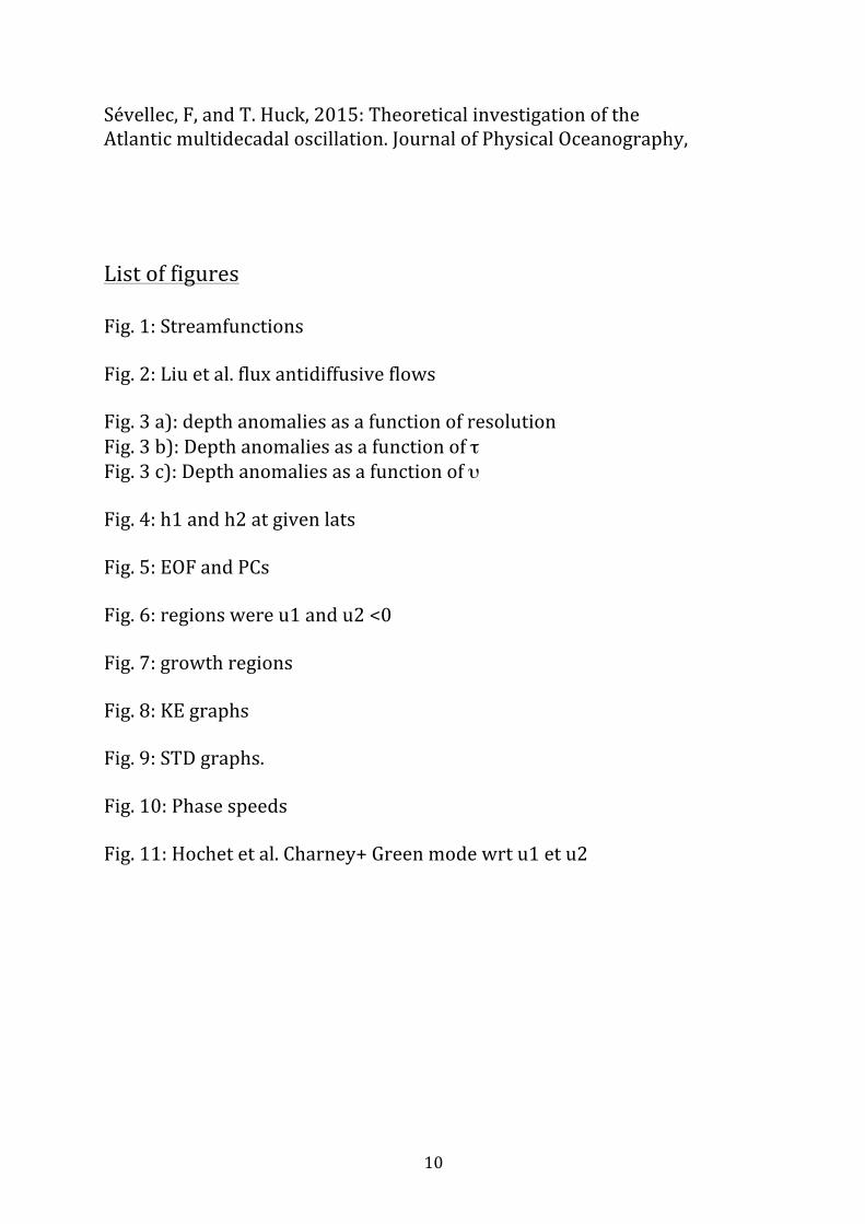
1.  Introduction    Using  a  2.5  layers  shallow  water  model  from  Jerome  Sirven  (Sirven  et  al,  in  review)  long-­‐term  baroclinic  instabilities  were  investigated  in  a  simplified  basin  resembling  the  north  Atlantic.  Sirven  et  al.  describes  decadal  variability,  centered  on  the  intergyre  region  resulting  from  the  outcropping  allowed  by  the  model.  Variability  from  seasonal  factors  appears  negligible,  however,  a  stronger  variability  in  the  region  of  instability  arises  from  long  term  phenomena  such  as  the  AMOC  and  the  NAO  (Sirven  et  al,  in  review).  Using  this  paper  as  the  basis  for  the  research,  the  model  was  further  simplified  in  order  to  determine  the  most  basic  configuration  under  which  interannual  instabilities  could  arise.    Following  Sirven’s  diagnostics,  non  linear  Rossby  waves  were  expected  to  develop  and  propagate  around  the  intergyre  region  following  the  Gulf  Stream  path.  Our  results  are  quite  different.  Indeed,  the  intergyre  region  defined  by  Sirven  et  al.  (in  review)  as  the  main  region  for  interannual  variability  is  here  of  lesser  importance.      2.  Model  Set  up    The  model  is  Shallow  water  with  2.5  layers,  the  third  layer  being  at  rest  and  of  infinite  depth.  The  diagnostics  are  made  using  variations  on  the  top  2  layers.  Coordinates  are  semi-­‐spherical  and  extend  from  15  to  55°N,  70°  to  10°W.  No  coastal  features  are  included  in  our  version  of  the  model,  as  opposed  to  Sirven  et  al.  original  configuration.  Furthermore,  the  wind  was  made  constant  instead  of  climatological.  No  overturning  circulation  was  prescribed.    The  model  circulation  follows  a  double  gyre  pattern  with  a  strong  western  boundary  current  as  shown  in  fig.  1.  This  circulation  holds  for  every  experiment  made,  with  the  volume  transport  varying  by  ±20  Sv  depending  mostly  on  τ.  A  permanent  gyre  can  be  seen  at  35°N  in  the  Western  Boundary  Current.      This  model  allows  the  thickness  of  the  first  layer  h1  to  shrink  towards  0  in  the  north  west  corner  of  the  basin  if  the  wind  forcing  was  sufficient,  resulting  in  the  second  layer  outcropping.  Under  climatological  winds  Sirven  et  al.  observed  outcropping,  however,  if  the  wind  stress  is  low,  no  outcropping  will  occur.  The  threshold  lies  in  between  0.06  and  0.08  kg.m-­‐

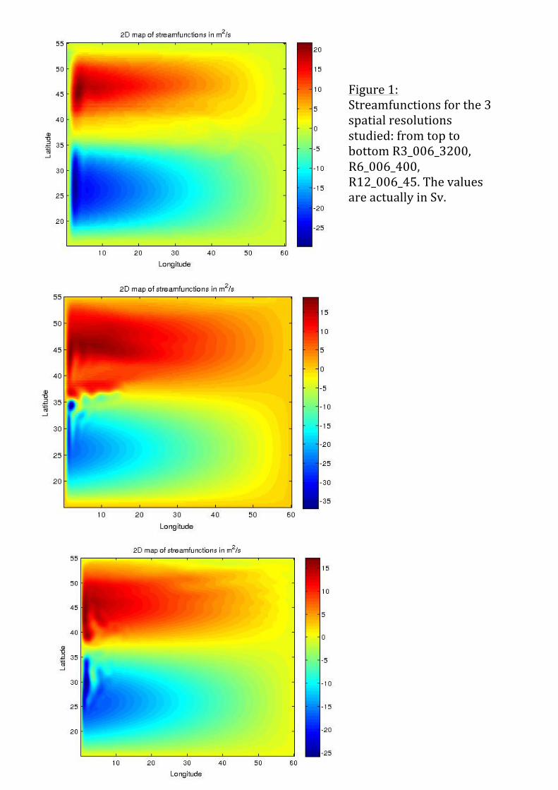
1.s-­‐2  .  The  size  of  the  outcropping  region  is  proportional  to  the  τ  value  used.  The  outcropping  is  maintained  through  the  use  of  antidiffusive  fluxes  as  

  3  

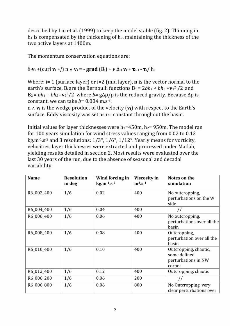
described  by  Liu  et  al.  (1999)  to  keep  the  model  stable  (fig.  2).  Thinning  in  h1  is  compensated  by  the  thickening  of  h2,  maintaining  the  thickness  of  the  two  active  layers  at  1400m.      The  momentum  conservation  equations  are:    ∂tvi  +(curl  vi  +f)  n  ∧  vi  =  -­‐  grad  (Bi)  +  v  ∆H  vi  +  τ i-­‐1  -­‐  τ i/  hi    

Where:  i=  1  (surface  layer)  or  i=2  (mid  layer),  n  is  the  vector  normal  to  the  earth’s  surface,  Bi  are  the  Bernoulli  functions  B1  =  2bh1  +  bh2  +v12  /2    and    B2  =  bh1  +  bh2  +  v22/2    where  b=  g∆ρ/ρ  is  the  reduced  gravity.  Because  ∆ρ  is  constant,  we  can  take  b=  0.004  m.s-­‐2.    n  ∧  vi    is  the  wedge  product  of  the  velocity  (vi)  with  respect  to  the  Earth’s  surface.  Eddy  viscosity  was  set  as  υ=  constant  throughout  the  basin.      Initial  values  for  layer  thicknesses  were  h1=450m,  h2=  950m.  The  model  ran  for  100  years  simulation  for  wind  stress  values  ranging  from  0.02  to  0.12  kg.m-­‐1.s-­‐2  and  3  resolutions:  1/3°,  1/6°,  1/12°.  Yearly  means  for  vorticity,  velocities,  layer  thicknesses  were  extracted  and  processed  under  Matlab,  yielding  results  detailed  in  section  2.  Most  results  were  evaluated  over  the  last  30  years  of  the  run,  due  to  the  absence  of  seasonal  and  decadal  variability.      Name   Resolution  

in  deg  Wind  forcing  in  kg.m-­‐1.s-­‐2  

Viscosity  in  m2.s-­‐1  

Notes  on  the  simulation  

R6_002_400   1/6   0.02   400   No  outcropping,  perturbations  on  the  W  side  

R6_004_400   1/6   0.04   400                    //  R6_006_400   1/6   0.06   400   No  outcropping,  

perturbations  over  all  the  basin  

R6_008_400   1/6   0.08   400   Outcropping,  perturbation  over  all  the  basin  

R6_010_400   1/6   0.10   400   Outcropping,  chaotic,  some  defined  perturbations  in  NW  corner  

R6_012_400   1/6   0.12   400   Outcropping,  chaotic    R6_006_200   1/6   0.06   200                      //  R6_006_800   1/6   0.06   800   No  Outcropping,  very  

clear  perturbations  over  

  4  

all  basin  R3_006_3200   1/3   0.06   3200   No  outcropping,  

perturbations  focused  in  mid  and  top  parts  

R3_008_3200   1/3   0.08   3200                  //  R12_006_45   1/12   0.06   45   Outcropping,  chaotic  

perturbations  over  all  basin  

R6_006_45_3mo   1/6   0.06   45   3  months  means.  Clearly  defined  eddies,  stable  perturbations  

   3.  Interannual  Variability    The  first  series  of  experiments  were  made  at  1/6°  resolution  for  all  τ  values  studied,  in  order  to  have  some  reference  points  for  further  experiments.  The  viscosity  parameter  υ  was  set  at  400m2.s-­‐1  ,  following  Sirven  et  al.  prescriptions.      Observed  large-­‐scale  anomalies  have  velocities  and  size  matching  Rossby  waves.  Those  Rossby  waves  propagating  westwards  were  observed,  regardless  of  the  τ  used  (fig.  3  b)),  emerging  from  the  north-­‐east  corner  of  the  basin  and  propagating  westwards.  Those  waves  exhibited  a  strong  tilt  and  had  a  very  repetitive  behaviour.    The  tilt  is  an  important  feature  as  it  creates  latitudinal  switch  is  the  sign  of  the  anomaly,  effectively  enhancing  it.  This  lead  us  to  believe  that  this  behaviour  was  robust,  however,  the  presence  of  those  waves  at  τ<0.06  lead  us  to  consider  them  as  not  being  an  inherent  consequence  of  the  outcropping  mechanism.      Longitudinal  sections  were  studied  at  high  latitudes  where  the  waves  seemed  predominant  showed  typical  phase  lag  between  h1  and  h2  (fig.  4).  This  behaviour  is  characteristic  of  baroclinic  instability  as  the  wave  propagation  in  a  given  layer  will  positively  feedback  the  propagation  in  the  other  layer.  The  amplitude  of  the  perturbations  varies  longitudinally,  indeed,  when  the  outcropping  region  was  small  enough  as  to  allow  perturbations  to  reach  the  western  side,  the  amplitude  of  h1  and  h2  anomalies  grew  before  diminishing  at  around  50°  W.  This  behaviour  held  for  all  experiments  at  1/6°.      Considering  the  characteristics  of  those  perturbations,  Empirical  Orthogonal  Functions  analysis  was  performed,  showing  percentage  of  variance  explained  close  to  80%  for  τ<0.10  (fig.5).  At  τ≥0.10,  the  perturbations  bore  no  more  tilt  and  the  EOF  values  shrank  to  30%  of  the  

  5  

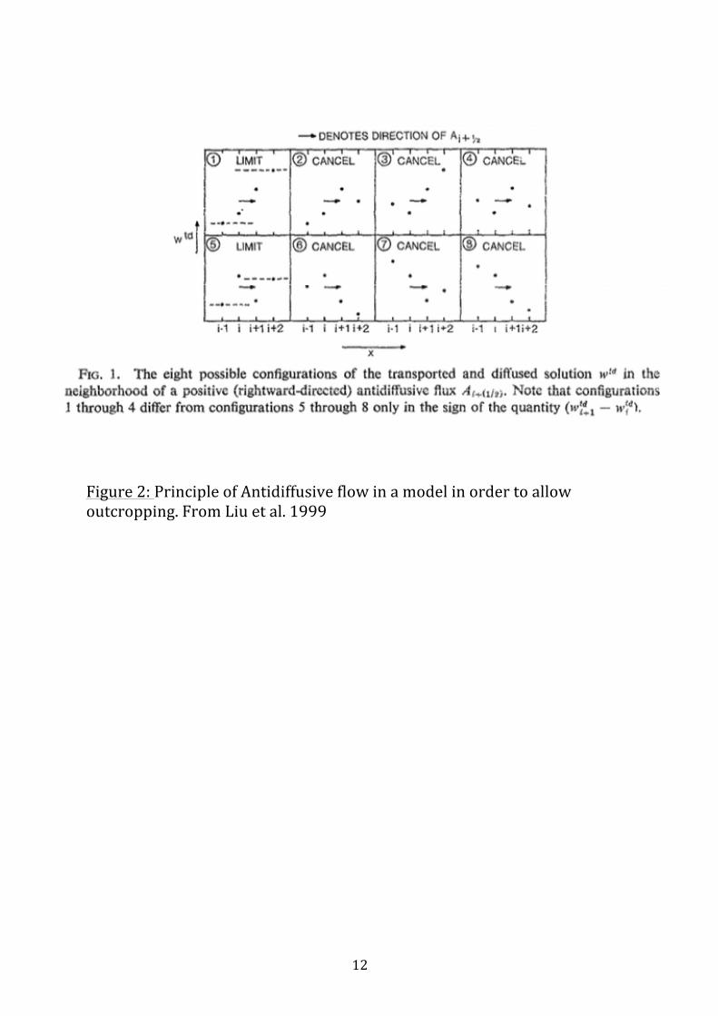
variance  explained.  PC  analysis  mirrored  this  behaviour,  with  chaotic  variations  arising  at  high  τ.    Emitting  the  hypothesis  that  those  perturbations  were  low  frequency  non  linear  Rossby  waves  as  described  by  Hochet  et  al.  (2015),  several  analysis  were  performed  to  determine  their  mode,  as  well  as  spatial  and  variability.    Zonal  velocities,  noted  u1  and  u2  for  the  top  and  mid  layer  respectively  were  westward  over  most  of  the  basin  (fig.6).  u1  <0  is  a  required  condition  for  baroclinic  instability  to  arise,  which  is  verified  in  our  case.      Using  Quasi-­‐Geostrophic  equations,  the  unstable  regions  were  analytically  identified    as  lying  in  the  north-­‐west  corner  of  the  basin  (fig.  7).  This  matched  the  observations  and  the  regions  at  which  the  imaginary  part  of  the  phase  speeds  was  ≠  ø.  This  is  particularly  striking  for  high  temporal  resolution.  However,  for  runs  at  lower  temporal  resolution,  growth  regions  were  seen  in  the  south-­‐west  corner  of  the  basin,  in  the  sub-­‐tropical  gyre,  as  well  as  in  the  north  east  corner.  This  is  opposite  to  the  initial  diagnostics  made  using  the  phase  speed  calculations.  Such  was  the  case  at  all  τ  values.  This  is  in  agreement  with  results  from  Liu  et  al.  1999  and  Cox  (1987),  however,  this  does  not  match  the  regions  where  the  anomalies  were  observed.  This  discrepancy  was  described  by  Hochet  et  al.  2015,  who  shows  that  analytical  methods  tend  to  yield  results  quite  different  from  observations.  The  reason  for  this  behaviour  has  not  been  established  and  is  thought  to  be  resulting  from  gaps  in  our  analytical  understanding  of  this  phenomenon.  Non-­‐linear  terms  and  approximations  made  could  be  a  potential  explanation  for  these  discrepancies    4.  Sensitivity  Experiments:    Experiments  were  carried  out  for  3  values  of  horizontal  viscosity  υ  at  1/6°:  200,  400(reference)  and  800m2.s-­‐1.  On  the  reference  experiment,  at  τ=0.12,  Rossby  waves  were  destroyed  before  they  could  reach  the  eastern  side  of  the  basin.  This  is  likely  due  to  the  meso-­‐scales  turbulences  (Huck  et  al.  2015).  Indeed,  large  changes  were  observed  when  modifying  the  υ  parameter:  when  this  parameter  was  increased  to  800,  all  turbulences  smaller  than  a  grid  point  were  destroyed,  further  amplifying  the  long-­‐term  anomalies.    However,  when  υ  was  decreased  to  200,  the  perturbations  were  propagating  chaotically,  without  tilt.    Experiments  were  also  made  at  higher  temporal,  then  spatial  resolution,  yielding  different  results.  As  expected,  for  1/12°  resolution,  meso-­‐scale  turbulences  destroyed  the  Rossby  waves,  in  the  same  manner  as  in  runs  

  6  

with  low  υ  values  or  high  τ  values.  As  a  result,  the  waves  lost  their  tilted  horizontal  structure,  however,  anomalies  could  still  be  seen,  exhibiting  the  same  behaviour  as  simulations  made  at  1/6°  with  τ=0.12.  At  means  calculated  every  3  months,  the  perturbations  were  more  clearly  defined  and  eddies  were  standing  out  along  the  northern  border  of  the  basin.      Important  changes  were  seen  at  1/3°.  Indeed,  reversed  perturbations  flowing  eastwards  are  seen  south  of  the  sub-­‐polar  gyre,  in  addition  to  Rossby  waves  propagating  westwards  north  of  the  gyre.    In  both  cases,  the  first  2  EOF  explain  only  10  to  20%  of  the  variance  observed,  depending  on  the  τ  value.      As  for  temporal  resolution  increase,  means  were  made  every  3  months,  hence  increasing  by  4  the  temporal  resolution.  This  translates  into  more  stable  Rossby  waves  crossing  the  basin,  with  the  first  2  EOFs  explaining  85%  of  the  variance  observed.  This  tends  to  prove  that  the  first  2  modes  are  driving  the  perturbations.      Over  every  experiments,  the  total  Kinetic  Energy  was  monitored  at  high  frequency  in  order  to  assess  the  impact  of  eddies.  Following  what  was  expected,  the  KE  increases  with  increasing  τ,  increasing  resolution  and  decreasing  υ  (fig.  8).  As  most  of  the  KE  in  the  ocean  is  stored  in  meso-­‐scale  eddies,  this  was  a  good  indicator.  Variations  in  KE  were  sinusoidal  when  the  anomalies  were  tilted  and  lost  clear  periodicity  when  τ  or  the  resolution  reached  critical  levels.      In  the  next  section,  we  will  attempt  to  explain  the  origin  of  the  observed  anomalies  and  explore  the  possibility  of  Green  modes  being  at  work  here.  Indeed,  Green  modes  are  the  result  of  coupling  between  the  Non-­‐Doppler  shift  mode,  resembling  the  first  mode  and  the  Advective  mode,  impacted  by  the  mean  flow,  hence  creating  instability  in  planetary  waves.  We  shall  also  highlight  discrepancies  between  our  expectations  from  theory  and  the  work  from  Hochet  et  al  and  Sirven  et  al.      5.  Interpretation  with  regards  to  Unstable  Rossby  Waves      As  mentioned  in  section  2,  our  results  were  quite  surprising,  due  to  the  apparent  robustness  of  the  Rossby  waves  to  varying  τ,  but  their  high  sensitivity  to  other  parameters  such  as  υ  or  the  resolution.  We  will  here  attempt  to  classify  these  perturbations  and  identify  their  propagating  mode.      

  7  

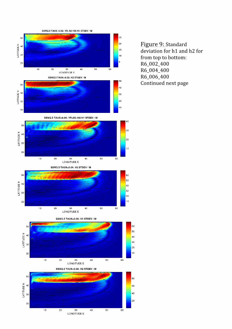
 At  first  order,  layer  thicknesses  standard  deviations  were  computed,  in  order  to  determine  regions  of  highest  perturbations’  influence.  As  τ  values  increase,  the  region  most  impacted  by  the  waves  drifts  towards  the  eastern  part  of  the  basin  (fig.  9).  2  reasons  may  explain  this:  the  outcropping  region  emerges  at  high  τ,  preventing  propagation  of  the  waves  in  the  top  layer,  hence  reducing  their  impact  on  the  second  layer.  Secondly,  as  τ  increases,  the  waves  form  faster  than  at  low  τ.      Rossby  waves  develop  in  presence  of  forcing  and  are  an  inherent  oceanic  behaviour.  They  are  the  restoring  mechanism  acting  against  isopycnal  slopes,  naturally  contained  in  the  mean  state.Those  waves  can  be  stable  or  unstable.  In  the  case  where  Rossby  waves  are  stable,  they  propagate  westwards  with  an  unchanging  wavelength  and  amplitude  due  to  initial  spin  up  or  changing  winds.  In  our  case,  Rossby  waves  show  varying  wavelength  with  longitude  and  their  amplitude  changes  (fig.4).  In  our  cases,  instabilities  arise  in  all  cases.  This  can  be  seen  from  the  imaginary  part  of  the  phase  speed  solution  (fig.  10).  As  mentioned  previously,  those  instabilities  are  fed  through  a  number  of  processes.  The  tilt  of  the  instabilities  creates  meridional  alternating  positive  and  negative  anomalies,  hence  promoting  perturbations  westwards  propagation  (Quentin  Jamet,  LPO,  Personal  comment).      On  vertical  level,  modes  are  defined  by  the  sign  of  u1  and  u2  with  respect  to  each  other.  If  they  are  of  the  same  sign,  the  first  mode  dominates  and  perturbations  are  unaffected  by  the  mean  flow.  If  the  two  have  different  sign,  the  second  mode  might  be  accelerated  by  the  mean  flow  to  the  point  where  it  couples  with  the  first  mode  and  creates  instabilities.  In  our  case,  u1  is  westwards  in  the  vast  majority  of  the  basin.  However,  as  seen  in  fig.  6,  there  are  regions  where  the  second  mode  is  promoted.      Depending  on  the  wavenumber  and  associated  growth  rate  ωi,  Rossby  waves  can  follow  different  propagation  modes.  At  the  scale  of  the  internal  Rossby  radius  of  deformation,  two  main  modes  are  generally  at  work:  Charney  mode  and  Green  mode.  As  detailed  by  Hochet  et  al.,  the  dominating  mode  is  a  function  of  several  parameters.  Representing  the  growth  rate  as  a  function  of  u1  and  u2  allows  us  to  identify  the  necessary  development  conditions  for  each  mode  (fig.  11).  In  our  case,  Green  mode  seems  to  be  favoured,  also  Charney  mode  cannot  be  set  apart  from  Green  mode.  Indeed,  the  relationship  between  the  wavenumber  kx  (in  rad-­‐1)  and  the  growth  rate  of  the  waves  showed  that  growth  was  selectively  significant  only  for  high  wavenumbers.  This  would  mean  that  Charney  mode  Rossby  waves  are  

  8  

being  destroyed  by  the  Laplacian  operator,  due  to  the  relationship  being  with  k2,  thus  promoting  exclusively  long-­‐term  and  large-­‐scale  variability  through  Green  mode,  due  to  Green  mode  waves  being  the  expression  of  the  least  damped  mode  generated  by  Rossby  waves.      During  early  calculations,  the  long  wave  approximation:  c=ω/k  was  used  to  infer  the  regions  of  growth  where  ωI  ≠0.  Eigenvalues  problem  was  solved  in  order  to  obtain  c  and  from  there  ω.  Under  the  long  wave  approximation,  results  correlated  well  with  the  obsertions  as  the  regions  were  located  in  the  North-­‐Western  part  of  the  basin,  precisely  where  Rossby  waves  seemed  to  grow  from  (fig.  2).  Further  calculations  involved  the  potential  vorticity  and  υ  in  the  calculations,  yielding  different  results,  with  a  shift  of  the  growth  regions  towards  the  south-­‐east  corner  of  the  basin.  Similar  discrepancies  were  observed  by  Hochet  et  al.  and  Liu  et  al.,  neither  providing  a  satisfactory  explanation  for  this  behaviour.      It  is  clear,  however,  that  due  to  υ’s  influence  the  positive  growth  rate  is  limited  to  low  k.  Could  it  be  then  that  the  growth  regions  observed  in  the  NW  corner  are  in  fact,  Charney  mode  perturbations?      We  verified  the  conditions  for  high  growth  rate  as  derived  by  Hochet  et  al.  in  the  case  of  2  layers  of  equal  thicknesses  under  constant  zonal  flows.  We  found  that  in  our  case,  the  boundaries  of  instability  were  different,  particularly  for  u2.  Indeed,  Hochet  et  al.  prescribe  boundaries  of  ±0.05  m/s,  while  we  had  growth  where  u2  either  <-­‐0.05  or    >0.  It  still  appears  safe  to  assume  that  the  perturbations  observed  are  indeed  Green  mode  Rossby  waves.      6.  Conclusion:    Low-­‐frequency  variability  in  an  idealised  Shallow  water  2.5  layers  model  was  studied  in  order  to  investigate  non-­‐linear  Rossby  waves  processes.  Due  to  the  modifications  brought  to  Sirven’s  model,  our  focus  shifted  from  the  Gulf  Stream’s  variability  to  low-­‐frequency  Rossby  waves.  The  absence  of  any  kind  of  seasonality  or  AMOC  type  of  process  means  our  variability  is  perfectly  periodic,  as  opposed  to  Sirven  et  al.’s  initial  research.  On  the  subject,  Sévellec  et  al.  (2015)  also  investigated  the  influence  of  Atlantic  Multidecadal  Oscillation  in  presence  of  vertical  AMOC  fluxes  and  provides  thorough  insight  on  the  influence  of  the  AMOC.  Moreover,  no  NW  corner  was  present,  potentially  impacting  the  outcropping  regions  and  influence.  Experiments  were  conducted  at  varying  resolutions  and  wind-­‐stress.  In  all  case,  non-­‐linear  Rossby  waves  developed  and  propagated  westwards,  

  9  

following  Green  mode  propagation  scheme.  Experiments  with  variability  in  wind  energy  input  would  be  valuable.  Further  investigation  of  the  vertical  mode  in  all  experiments  should  also  be  done.  It  should  be  established  which  parameters  amongst  velocity,  vorticity,  β  and  υ  has  the  most  influence  on  the  variability  observed,  by  setting  them  all  at  their  mean  values  and  letting  one  at  a  time  follow  its  variations.  The  double  gyre  circulation  pattern  might  be  a  key  parameter  for  the  observed  instabilities  (Ben  Jelloul  &  Huck  2003).      References    Ben  Jelloul,  M.,  and  T.  Huck,  2003:  Basin  modes  interactions  and    selection  by  the  mean  flow  in  a  reduced-­‐gravity  quasigeostrophic  model.      Cox,  M.  D.,  1987:  An  eddy  resolving  numerical  model  of  the  ventilated    thermocline:  Time  dependence.      Hochet,  Antoine,  2015:  Étude  des  courants  océaniques  transitoires  de    grande  échelle:  structure  verticale,  interaction  avec  la  topographie  et    le  courant  moyen,  stabilité.  PhD  manuscript,  Université  de  Bretagne    Occidentale,  Brest,  France.    Hochet,  A.,  T.  Huck,  A.  Colin  de  Verdière,  2015:  Large  scale  baroclinic    instability  of  the  mean  oceanic  circulation:  a  local  approach.      Huck,  T.,  O.  Arzel,  F.  Sévellec,  2015:  Multidecadal  variability  of  the    overturning  circulation  in  presence  of  eddy  turbulence.  \JPO{45}  (1)    157-­‐173,  doi:  http://dx.doi.org/10.1175/JPO-­‐D-­‐14-­‐0114.1  .    Liu,  Z.,  1999:  Planetary  wave  modes  in  the  thermocline:    Non-­‐Doppler-­‐shift  mode,  advective  mode  and  Green  mode.      Sévellec,  F,  and  T.  Huck,  2015:  Theoretical  investigation  of  the    Atlantic  multidecadal  oscillation.  Journal  of  Physical  Oceanography,      Sirven,  J.,  S.  Février,  C.  Herbaut,  2015:  Low  frequency  variability  of    the  separated  western  boundary  current  in  response  to  a  seasonal  wind    stress  in  a  2.5  layer  model  with  outcropping.      Huck,  T.,  O.  Arzel,  F.  Sévellec,  2015:  Multidecadal  variability  of  the    overturning  circulation  in  presence  of  eddy  turbulence    

  10  

Sévellec,  F,  and  T.  Huck,  2015:  Theoretical  investigation  of  the    Atlantic  multidecadal  oscillation.  Journal  of  Physical  Oceanography,            List  of  figures      Fig.  1:  Streamfunctions      Fig.  2:  Liu  et  al.  flux  antidiffusive  flows    Fig.  3  a):  depth  anomalies  as  a  function  of  resolution  Fig.  3  b):  Depth  anomalies  as  a  function  of  τ  Fig.  3  c):  Depth  anomalies  as  a  function  of  υ    Fig.  4:  h1  and  h2  at  given  lats    Fig.  5:  EOF  and  PCs    Fig.  6:  regions  were  u1  and  u2  <0    Fig.  7:  growth  regions    Fig.  8:  KE  graphs    Fig.  9:  STD  graphs.    Fig.  10:  Phase  speeds      Fig.  11:  Hochet  et  al.  Charney+  Green  mode  wrt  u1  et  u2                  

  11  

 Figure  1:  Streamfunctions  for  the  3  spatial  resolutions  studied:  from  top  to  bottom  R3_006_3200,  R6_006_400,  R12_006_45.  The  values  are  actually  in  Sv.          

                                                         

  12  

 

     Figure  2:  Principle  of  Antidiffusive  flow  in  a  model  in  order  to  allow  outcropping.  From  Liu  et  al.  1999                                            

  13  

 Figure  3  a)  Depth  anomalies  at  the  last  year  of  each  simulation.  From  top  to  bottom:  R3_006_3200,  R6_006_400  R12_006_45                                            

                       

  14  

Figure  3  b)  On  this  page,  top  to  bottom:    R6_002_400,  R6_004_400,  R6_006_400  Continued  next  page                                                                  

  15  

On  this  page:  top  to  bottom,  R6_008_400,  R6_010_400,  R6_012_400                                                                      

  16  

Figure  3  c)  On  this  page,  top  to  bottom:    R6_006_200  R6_006_800                                                              

  17  

Figure  4:  Longitudinal  profiles  of  h1  and  h2  anomalies.  From  top  to  bottom:  R3_006_3200,  R6_006_400  R12_006_45                                                                

  18  

Figure  5:  EOF  and  PC  analysis  for  top:  R6_006_400  bottom:  R3_006_3200  These  2  illustrate  well  the  situation  for  well  defined  perturbations  and  poorly  defined  perturbations.          

                                 

  19  

Figure  6:  Regions  where  Mean  zonal  velocities  flows  are  <0  in  R6_008_400.  Very  little  variability  was  observed  over  all  experiments.  These  regions  indicate  regions  of  potential  instability  growth.                                  

  20  

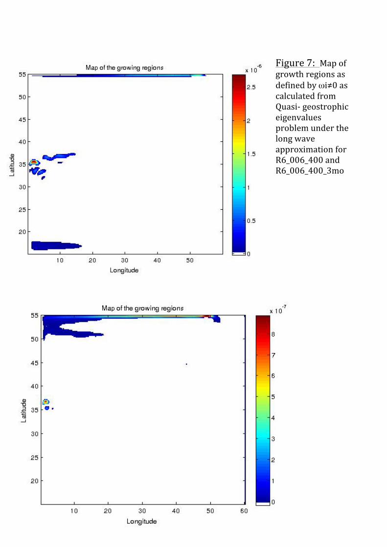
 Figure  7:    Map  of  growth  regions  as  defined  by  ωi≠0  as  calculated  from  Quasi-­‐  geostrophic  eigenvalues  problem  under  the  long  wave  approximation  for  R6_006_400  and  R6_006_400_3mo                        

                                       

  21  

Figure  8:  Kinetic  Energy  over  time  for:  top  to  bottom:  R3_008_3200  R6_006_400  R12_006_45    See  next  page  for  influence  of  τ  and  υ  on  R=1/6  and  υ=400          

                               

                       

  22  

 

  23  

   Figure  9:  Standard  deviation  for  h1  and  h2  for  from  top  to  bottom:    R6_002_400  R6_004_400  R6_006_400  Continued  next  page          

                                                       

  24  

R6_008_400    R6_010_400  R6_012_400                                                      

                     

  25  

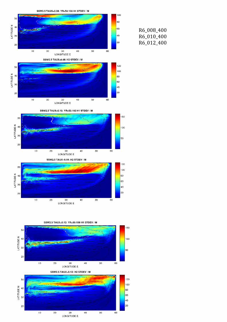
Figure  10:  Real  and  imaginary  part  of  the  long  Rossby  waves  phase  speed  for  R6_006_400  The  black  contours  on  the  real  part  indicate  regions  where  iC≠0.  Note  the  differences  in  growth  region  with  Fig.7.            

                                             

  26  

 

   Figure  11:  Growth  time  of  large  scale  mode  in  a  2.5  layers  Shallow  Water  model  as  a  function  of  u1  and  u2  at  lat=30°N  for  h1=h2=200m.  From  Hochet  et  al.  These  2015.