interpolating vancouver's daily ambient pm10 field

ENVIRONMETRICS

Environmetrics 1999^ 00]540Ð552

Received 01 October 0888Copyright Þ 1999 John Wiley + Sons\ Ltd[ Revised 17 February 1999

Interpolating Vancouver|s daily ambient PM09 _eld

Li Sun0\ James V[ Zidek0�\ Nhu D[ Le1 and Halu¼k O� zkaynak2

0 Department of Statistics\ University of British Columbia\ Vancouver\ British Columbia\ Canada1 BC Cancer A`ency\ Vancouver\ British Columbia\ Canada

2 US Environmental Protection A`ency\ U[S[A[

SUMMARY

In this article we develop a spatial predictive distribution for the ambient spaceÐtime response _eld of dailyambient PM09 in Vancouver\ Canada[ Observed responses have a consistent temporal pattern from onemonitoring site to the next[ We exploit this feature of the _eld by adopting a response model with twocomponents\ a common deterministic trend across all sites plus a stochastic residual[ We are thereby ableto whiten the temporal residuals without losing much of the spatial correlation in the original log!trans!formed series[ This in turn enables us to develop an e}ective spatial predictive distribution for these residualsat unmonitored sites[ By transforming the predicted residuals back to the original data scales\ we can imputeVancouver|s daily PM09 _eld for purposes such as human exposure and health impacts analysis[ CopyrightÞ 1999 John Wiley + Sons\ Ltd[

KEY WORDS] PM09^ space!models^ autoregressive processes^ spatial interpolation^ monitoring networks^spatial correlation

0[ INTRODUCTION

This paper follows that of Li et al[ "0888# analyzing the hourly PM09 _eld over the GreaterVancouver Regional District "GVRD#[ It bypasses problems arising from the spatial complexityof that _eld by turning from hourly to daily averages of this important air pollutant[ Thatsolution will be quite satisfactory for many purposes[ We confront the more di.cult problem ofpredicting hourly averages in a sequel to this paper[

Interest in this pollutant derives from the recognition that elevated levels are associated withacute negative health impacts[ A panel of experts appointed by the U[K[ Department of theEnvironment\ Transport and the Regions concludes "http]::www[environment[detr[gov[uk:airq:aqs:particle:\ paragraph 14#]

of PM09 and health e}ects\ [ [ [ that the higher the concentration of particles\ the greater

� Correspondence to] J[ V[ Zidek\ Department of Statistics\ University of British Columbia\ 5245 Agricultural Road\Vancouver\ BC\ Canada V5T 0Z1[

L[ SUN ET AL[

Copyright Þ 1999 John Wiley + Sons\ Ltd[ Environmetrics 1999^ 00]540Ð552

541

Figure 0[ Locations of the 09 PM09 monitoring stations in Vancouver[

the e}ect on the health of the population and conversely\ the lower the concentration\ thesmaller the e}ect[

Li et al[ "0888# analyze hourly ambient PM09 concentrations collected in the Vancouver areafrom 0883 to 0885[ Data come from 09 monitoring stations in the GVRD "see Figure 0 andTable 0#\ di}erent stations starting operation at di}erent times[

Table 0[ Location of PM09 monitoring sites[

Site Location Latitude Longitude

0 Rocky Point Park 38[17972 011[73701 Kitsilano 38[15149 012[05142 Kensington Park 38[16806 011[85863 Surrey East 38[02167 011[58224 Richmond South 38[03083 012[09675 Burnaby South 38[10556 011[87226 North Delta 38[04722 011[89977 Langley 38[98500 011[45538 Abbotsford Downtown 38[93833 011[1814

09 Chilliwack Airport 38[04000 010[8358

SPATIAL PREDICTIVE DISTRIBUTION TECHNIQUE


542

Tapered Element Oscillating Microbalance "TEOM# monitors generated the data\ the data weuse to construct the simple daily averages[ "These {continuous| monitors use a tapered quartzelement of conical shape[ A detachable impervious _lter is connected at the larger end and air isdrawn onto that _lter[ The element oscillates at its resonant frequency when an electrical currentis passed through the element[ However\ as the particle loading builds up\ that frequency changesunless the current is altered to maintain the resonant frequency[ The change in current neededprovides the surrogate measure of particulate concentration that gets converted and averagedto yield the measurements[ "Environmental Health Department\ Warwick District Council\http]::www[warwickdceh[demon[co[uk:equip[htm èDataCapture#[

The analysis of Li et al[ "0888# was to be a prelude to the development of a spatial predictionmethodology for imputing unmeasured levels of PM09 at 188 additional locations[ In this paper\we deal with the problem of predicting unmeasured daily average values\ the more subtle problemof predicting hourly averages being left to a sequel[

In the next section\ we model the daily average concentration _elds for PM09[ Section 2 presentsa spatial predictive distribution of unmeasured values[ In Section 3\ we investigate the relativecoverage frequencies of the predictive credibility intervals derived from our predictive distri!butions[ The paper concludes with a discussion of our _ndings[

1[ LOG PM09 CONCENTRATIONS IN VANCOUVER

In this section we show that an AR"0# model describes the daily averages of de!trended logPM09 concentrations in Vancouver quite well[ Daily average values derive from hourly PM09

measurements collected by a network of TEOM monitors across the GVRD in 0885[ One station"Abbortsford# had just over two months of missing values and for our analysis these wereimputed using spatial regression[ Otherwise only 05 daily values were missing at random out ofthe 255×8 station!days in 0885[ These missing values were imputed as the average for all otherstations on the same day[

For any location x and day d\ let X"x\d# represent the daily log PM09 average concentration"mg:m2#[ Furthermore\ let S"d# represent the overall trend in these spatial averages for day d\ i[e[

S"d# �m?¦Dday¦Wweek

where m?�m¦"H0¦= = =¦H13#:13 is the overall mean e}ect in the daily model\ Dday and Wweek

are the daily "day!of!week# and weekly "week!of!year# e}ects\ respectively[ Here m represents theaverage over all sites\ Hhour\ the corresponding average for hour�0\ [ [ [ \ 13 once m has beensubtracted from all responses\ Dday\ the corresponding average for day�0\ [ [ [ \ 6 once m? hasbeen subtracted from all responses\ Wweek\ the corresponding average for week�0\ [ [ [ \ 41 onceboth m? and Dday have been subtracted from all responses[

To explore the nature of temporal variation in the daily de!trended residualsD"x\d# �X"x\d#−S"d# we estimated at each monitoring site x the auto!correlation in the D!series[ The resulting auto!correlation function plots indicate a strong _rst order auto!correlationat each site "browse http]::home[stat[ubc[ca:½jim:pubs:pmday to see these plots and more detailfor the analysis below#[ The corresponding partial auto!correlation function plots con_rm thisobservation[ The latter also suggest we can rule out a moving average component in the series[The consistency across monitoring sites seen in the plots led us to adopt a single time!series

L[ SUN ET AL[


543

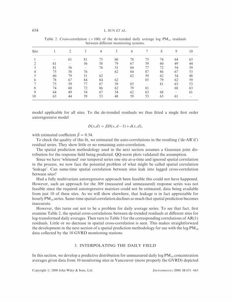
Table 1[ Cross!correlation "×099# of the de!trended daily average log PM09 residualsbetween di}erent monitoring systems[

Site 0 1 2 3 4 5 6 7 8 09

0 Ð 50 70 64 59 67 64 63 53 521 50 Ð 45 47 68 56 48 59 38 332 70 45 Ð 65 40 73 66 61 43 483 64 47 65 Ð 51 73 76 75 56 424 59 68 40 51 Ð 51 48 51 43 375 67 56 73 73 51 Ð 74 68 51 486 64 48 66 76 48 74 Ð 70 52 427 63 59 61 75 51 68 70 Ð 57 528 53 38 43 56 43 51 52 57 Ð 50

09 52 33 48 42 37 48 42 52 50 Ð

model applicable for all sites[ To the de!trended residuals we thus _tted a single _rst orderautoregressive model

D"x\d# �bD"x\ d−0#¦d"x\ d#\

with estimated coe.cient b¼ � 9[23[To check the quality of this _t\ we estimated the auto!correlations in the resulting "{de!AR|d|#

residual series[ They show little or no remaining auto!correlation[The spatial prediction methodology used in the next section assumes a Gaussian joint dis!

tribution for the response _eld being predicted[ QQ!norm plots validated the assumption[Since we have {whitened| our temporal series one site at!a!time and ignored spatial correlation

in the process\ we now face the potential problem of what might be called spatial correlation{leakage|[ Can same!time spatial correlation between sites leak into lagged cross!correlationbetween sites<

Had a fully multivariate autoregressive approach been feasible this could not have happened[However\ such an approach for the 298 "measured and unmeasured# response series was notfeasible since the required autoregressive matrices could not be estimated\ data being availablefrom just 09 of these sites[ As we will show elsewhere\ that leakage is in fact appreciable forhourly PM09 series[ Same!time spatial correlation declines so much that spatial prediction becomesinaccurate[

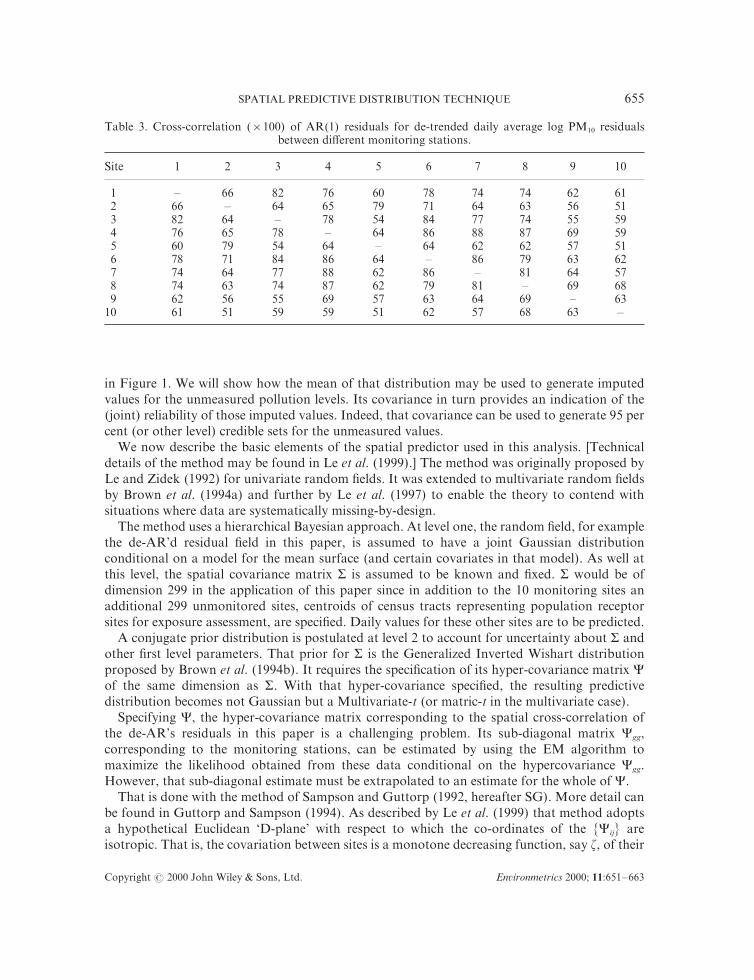
However\ this turns out not to be a problem for daily average series[ To see that fact\ _rstexamine Table 1\ the spatial cross!correlations between de!trended residuals at di}erent sites forlog!transformed daily averages[ Then turn to Table 2 for the corresponding correlations of AR"0#residuals[ Little or no decrease in spatial cross!correlation is seen[ This makes straightforwardthe development in the next section of a spatial prediction methodology for use with the log PM09

data collected by the 09 GVRD monitoring stations[

2[ INTERPOLATING THE DAILY FIELD

In this section\ we develop a predictive distribution for unmeasured daily log PM09 concentrationaverages given data from 09 monitoring sites in Vancouver "more properly the GVRD# depicted



544

Table 2[ Cross!correlation "×099# of AR"0# residuals for de!trended daily average log PM09 residualsbetween di}erent monitoring stations[

Site 0 1 2 3 4 5 6 7 8 09

0 Ð 55 71 65 59 67 63 63 51 501 55 Ð 53 54 68 60 53 52 45 402 71 53 Ð 67 43 73 66 63 44 483 65 54 67 Ð 53 75 77 76 58 484 59 68 43 53 Ð 53 51 51 46 405 67 60 73 75 53 Ð 75 68 52 516 63 53 66 77 51 75 Ð 70 53 467 63 52 63 76 51 68 70 Ð 58 578 51 45 44 58 46 52 53 58 Ð 52

09 50 40 48 48 40 51 46 57 52 Ð

in Figure 0[ We will show how the mean of that distribution may be used to generate imputedvalues for the unmeasured pollution levels[ Its covariance in turn provides an indication of the"joint# reliability of those imputed values[ Indeed\ that covariance can be used to generate 84 percent "or other level# credible sets for the unmeasured values[

We now describe the basic elements of the spatial predictor used in this analysis[ ðTechnicaldetails of the method may be found in Le et al[ "0888#[Ł The method was originally proposed byLe and Zidek "0881# for univariate random _elds[ It was extended to multivariate random _eldsby Brown et al[ "0883a# and further by Le et al[ "0886# to enable the theory to contend withsituations where data are systematically missing!by!design[

The method uses a hierarchical Bayesian approach[ At level one\ the random _eld\ for examplethe de!AR|d residual _eld in this paper\ is assumed to have a joint Gaussian distributionconditional on a model for the mean surface "and certain covariates in that model#[ As well atthis level\ the spatial covariance matrix S is assumed to be known and _xed[ S would be ofdimension 188 in the application of this paper since in addition to the 09 monitoring sites anadditional 188 unmonitored sites\ centroids of census tracts representing population receptorsites for exposure assessment\ are speci_ed[ Daily values for these other sites are to be predicted[

A conjugate prior distribution is postulated at level 1 to account for uncertainty about S andother _rst level parameters[ That prior for S is the Generalized Inverted Wishart distributionproposed by Brown et al[ "0883b#[ It requires the speci_cation of its hyper!covariance matrix Cof the same dimension as S[ With that hyper!covariance speci_ed\ the resulting predictivedistribution becomes not Gaussian but a Multivariate!t "or matric!t in the multivariate case#[

Specifying C\ the hyper!covariance matrix corresponding to the spatial cross!correlation ofthe de!AR|s residuals in this paper is a challenging problem[ Its sub!diagonal matrix C``\corresponding to the monitoring stations\ can be estimated by using the EM algorithm tomaximize the likelihood obtained from these data conditional on the hypercovariance C``[However\ that sub!diagonal estimate must be extrapolated to an estimate for the whole of C[

That is done with the method of Sampson and Guttorp "0881\ hereafter SG#[ More detail canbe found in Guttorp and Sampson "0883#[ As described by Le et al[ "0888# that method adoptsa hypothetical Euclidean {D!plane| with respect to which the co!ordinates of the "Cij# areisotropic[ That is\ the covariation between sites is a monotone decreasing function\ say z\ of their

L[ SUN ET AL[


545

D!plane distances[ The method estimates that monotone function and the D!plane location co!ordinates associated with each of the monitored sites di � "di0\di1# for site i with geographical co!ordinates gi � "`i0\`i1#[ The method relates the "di# to the "gi# through thin plate smoothingsplines f by means of dj � fj"g#\ j�0\ 1[ These splines are _tted to the D! and G!plane co!ordinatepairs for the gauged or measured sites\ the degree of _t depending on the so!called smoothingparameter l or {lambda| in _gures below[ The "di# are then replaced by the _ts "f"gi##\ wheref� " f0\ f1#[

Large values of that parameter will entail poor G! to D!plane co!ordinate _ts[ However\ thosesplines will more faithfully maintain the character of the G!plane and lead to simplicity ofinterpretation of the results of the analysis[ At the other extreme\ small values can lead to splinesthat twist the G!plane into unrecognizable form while ensuring a good _t to the estimated D!plane co!ordinates[

The choice of this parameter is subjective[ {Small| tends to be better because the co!ordinatesof the estimated C`` will tend to be more closely isotropic in the f image of the G!plane[ On theother hand\ some smoothing is desirable to achieve a degree of interpretability in the relationshipbetween the resulting plane and its G counterpart[

Once f has been speci_ed\ the required extension of the estimated C`` to C can easily be made[Represent the G!plane co!ordinates of sites i and j corresponding to Cij\ gi and gj\ by their fimages in the D!plane di � f"gi# and dj � f"gj#[ Finally\ estimate Cij by z">di−dj>#[

In practice the SG method is implemented through the so!called {variogram| in exactly thesame way as described above for the covariance[ In general\ for a random _eld Z"x#\ the latteris de_ned for locations x and x? by VarðZ"x#−Z"x?#Ł[ It is closely related to the covariance andlike the latter is easily estimated when independent replicates of Z over time are available at thetwo sites[ The estimate is simply the sample average of squared di}erences in Z between the twosites[ Software has been developed for implementing the SG method and we are indebted toProfessors Guttorp and Sampson for supplying the version used here[ Estimates of C can easilybe found from estimates of the variogram[

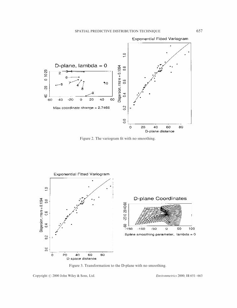
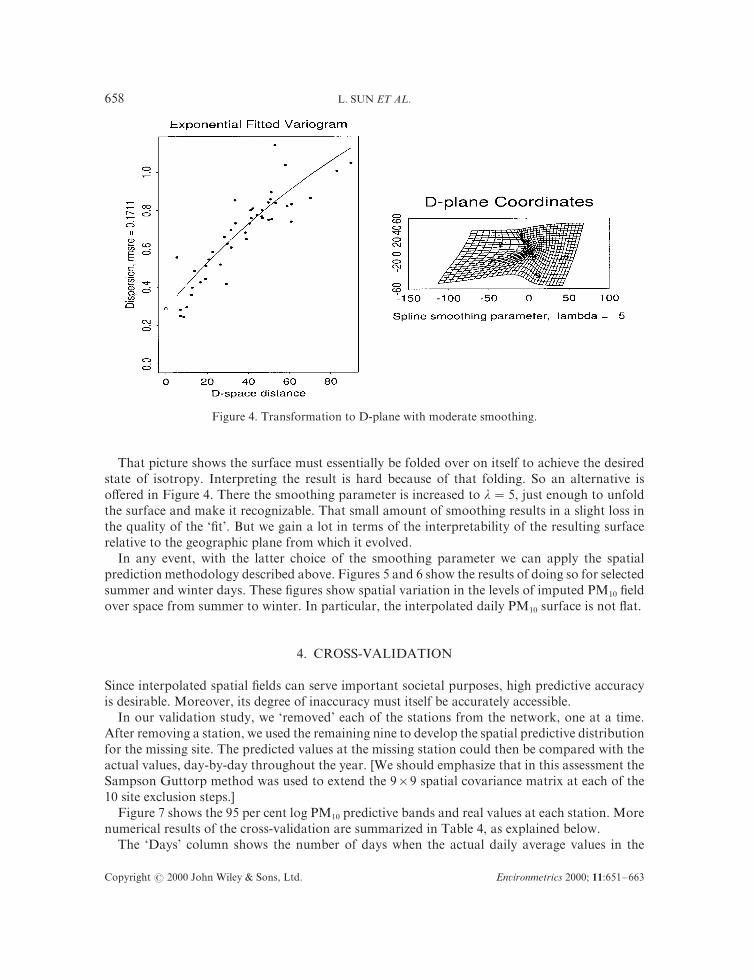
For any pair of the 09 monitored sites in our application\ we estimate the variogram in themanner described above[ The resulting 34 estimates "for all possible site pairs# are assigned D!plane co!ordinates in the manner described above[ Each of the 34 estimates can be plotted againstthe D!plane distance separating them[ Of course\ the D!plane distance between them will dependon the selected size of the spline smoothing parameter[ However\ if no smoothing is used\ onecan see that plot in the right hand panel of Figure 1[ The scatter plot shows 34 plotted variogramestimates and the best _tting exponential variogram plotted against them[ ðAn anonymous refereehas pointed out that the variogram we have chosen on the basis of its goodness!of!_t implies therandom _eld is merely continuous and not di}erentiable[ However\ since we do not have a priorigrounds for assuming process di}erentiability\ we accept the best _tting variogram on pragmaticgrounds[Ł

The left!hand panel of the same _gure shows two monitoring sites è4 "Richmond# and è8"Abbotsford# that must move away from the remaining eight sites to achieve an isotropiccorrelation _eld[ In other words\ these two stations tend to be un!correlated with the rest\ somust be moved away in the D!plane to achieve inter!station distances commensurate with thelow spatial cross!correlations they have with the rest[

Figure 2 o}ers a di}erent view of the same situation[ The scatter plot in that _gure is identicalto that in Figure 1[ However\ it shows in a more pictorial way how the "geographic# G!planemust be folded to re!organize the G!surface so as to make the variogram separation betweensites correspond to their D!plane distances[



546

Figure 1[ The variogram _t with no smoothing[

Figure 2[ Transformation to the D!plane with no smoothing[

L[ SUN ET AL[


547

Figure 3[ Transformation to D!plane with moderate smoothing[

That picture shows the surface must essentially be folded over on itself to achieve the desiredstate of isotropy[ Interpreting the result is hard because of that folding[ So an alternative iso}ered in Figure 3[ There the smoothing parameter is increased to l�4\ just enough to unfoldthe surface and make it recognizable[ That small amount of smoothing results in a slight loss inthe quality of the {_t|[ But we gain a lot in terms of the interpretability of the resulting surfacerelative to the geographic plane from which it evolved[

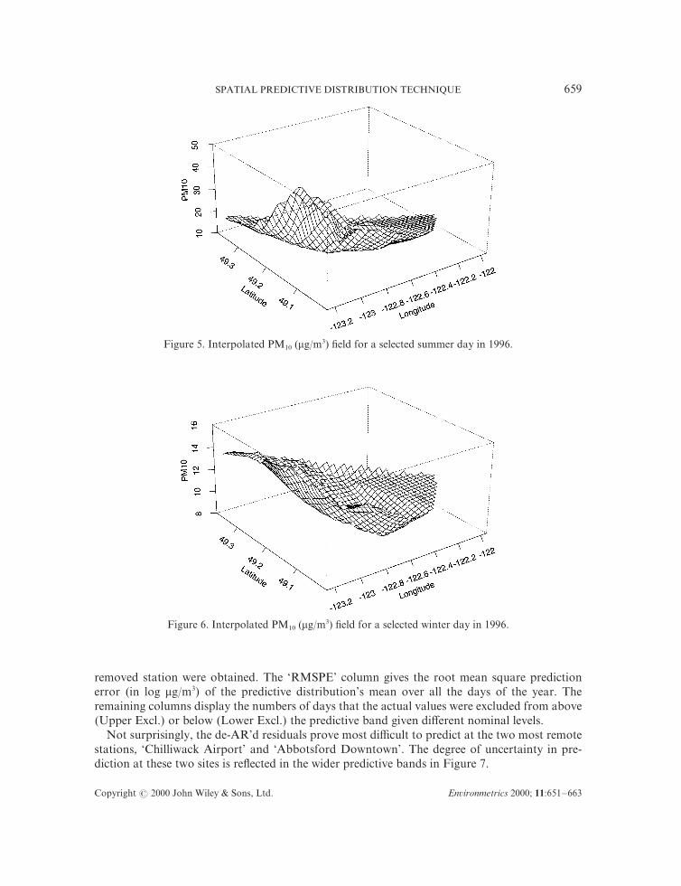
In any event\ with the latter choice of the smoothing parameter we can apply the spatialprediction methodology described above[ Figures 4 and 5 show the results of doing so for selectedsummer and winter days[ These _gures show spatial variation in the levels of imputed PM09 _eldover space from summer to winter[ In particular\ the interpolated daily PM09 surface is not ~at[

3[ CROSS!VALIDATION

Since interpolated spatial _elds can serve important societal purposes\ high predictive accuracyis desirable[ Moreover\ its degree of inaccuracy must itself be accurately accessible[

In our validation study\ we {removed| each of the stations from the network\ one at a time[After removing a station\ we used the remaining nine to develop the spatial predictive distributionfor the missing site[ The predicted values at the missing station could then be compared with theactual values\ day!by!day throughout the year[ ðWe should emphasize that in this assessment theSampson Guttorp method was used to extend the 8×8 spatial covariance matrix at each of the09 site exclusion steps[Ł

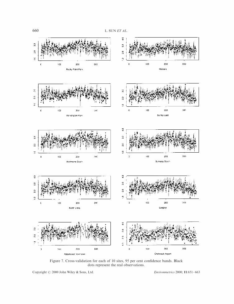
Figure 6 shows the 84 per cent log PM09 predictive bands and real values at each station[ Morenumerical results of the cross!validation are summarized in Table 3\ as explained below[

The {Days| column shows the number of days when the actual daily average values in the



548

Figure 4[ Interpolated PM09 "mg:m2# _eld for a selected summer day in 0885[

Figure 5[ Interpolated PM09 "mg:m2# _eld for a selected winter day in 0885[

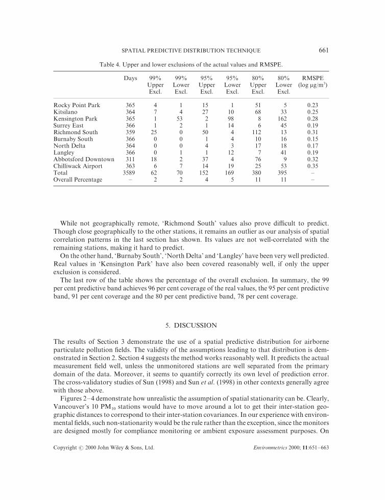
removed station were obtained[ The {RMSPE| column gives the root mean square predictionerror "in log mg:m2# of the predictive distribution|s mean over all the days of the year[ Theremaining columns display the numbers of days that the actual values were excluded from above"Upper Excl[# or below "Lower Excl[# the predictive band given di}erent nominal levels[

Not surprisingly\ the de!AR|d residuals prove most di.cult to predict at the two most remotestations\ {Chilliwack Airport| and {Abbotsford Downtown|[ The degree of uncertainty in pre!diction at these two sites is re~ected in the wider predictive bands in Figure 6[

L[ SUN ET AL[


559

Figure 6[ Cross!validation for each of 09 sites\ 84 per cent con_dence bands[ Blackdots represent the real observations[



550

Table 3[ Upper and lower exclusions of the actual values and RMSPE[

Days 88) 88) 84) 84) 79) 79) RMSPEUpper Lower Upper Lower Upper Lower "log mg:m2#Excl[ Excl[ Excl[ Excl[ Excl[ Excl[

Rocky Point Park 254 3 0 04 0 40 4 9[12Kitsilano 253 6 3 16 09 57 22 9[14Kensington Park 254 0 42 1 87 7 051 9[17Surrey East 255 0 1 0 03 5 34 9[08Richmond South 248 14 9 49 3 001 02 9[20Burnaby South 255 9 9 0 3 09 05 9[04North Delta 253 9 9 3 2 06 07 9[06Langley 255 9 0 0 01 6 30 9[08Abbotsford Downtown 200 07 1 26 3 65 8 9[21Chilliwack Airport 252 5 6 03 08 14 42 9[24Total 2478 51 69 041 058 279 284 ÐOverall Percentage Ð 1 1 3 4 00 00 Ð

While not geographically remote\ {Richmond South| values also prove di.cult to predict[Though close geographically to the other stations\ it remains an outlier as our analysis of spatialcorrelation patterns in the last section has shown[ Its values are not well!correlated with theremaining stations\ making it hard to predict[

On the other hand\ {Burnaby South|\ {North Delta| and {Langley| have been very well predicted[Real values in {Kensington Park| have also been covered reasonably well\ if only the upperexclusion is considered[

The last row of the table shows the percentage of the overall exclusion[ In summary\ the 88per cent predictive band achieves 85 per cent coverage of the real values\ the 84 per cent predictiveband\ 80 per cent coverage and the 79 per cent predictive band\ 67 per cent coverage[

4[ DISCUSSION

The results of Section 2 demonstrate the use of a spatial predictive distribution for airborneparticulate pollution _elds[ The validity of the assumptions leading to that distribution is dem!onstrated in Section 1[ Section 3 suggests the method works reasonably well[ It predicts the actualmeasurement _eld well\ unless the unmonitored stations are well separated from the primarydomain of the data[ Moreover\ it seems to quantify correctly its own level of prediction error[The cross!validatory studies of Sun "0887# and Sun et al[ "0887# in other contexts generally agreewith those above[

Figures 1Ð3 demonstrate how unrealistic the assumption of spatial stationarity can be[ Clearly\Vancouver|s 09 PM09 stations would have to move around a lot to get their inter!station geo!graphic distances to correspond to their inter!station covariances[ In our experience with environ!mental _elds\ such non!stationarity would be the rule rather than the exception\ since the monitorsare designed mostly for compliance monitoring or ambient exposure assessment purposes[ On

L[ SUN ET AL[


551

the other hand\ these SG estimated spatial correlations are subject to considerable samplingerrors\ a subject to be investigated in a forthcoming paper[

Note that the interpolated surfaces are not ~at[ Their irregularity comes in the _rst instancefrom variation in the daily levels of PM09 at the 09 monitored stations^ the interpolated valuesmust approximate the actual values at monitored stations\ the {nugget e}ect| being quite small[However\ between stations the interpolated surface must regress towards the mean[ The inevitable{regression!toward!the!mean| e}ect thus contributes to the impression of irregularity of theambient particulate pollution _eld[

This _nding shows that this interpolator under!predicts the extreme values in the pollution_eld[ This could be quite signi_cant in the analysis of population exposures and human healthe}ects\ for example[ Here the contrast in pollution levels between geographical sub!regionsshould be preserved to maximize the power of the method to detect association between airpollution exposures and health outcomes\ such as admission to hospitals for respiratorymorbidity[ However\ because we have based our interpolation methodology on a spatial pre!dictive distribution\ the methodology recognizes these extremes "implicitly# and allows for ouruncertainty about their size in health impact analysis[

To conclude\ we consider one other issue concerning the strategy we have developed for spaceÐtime analysis[ That issue revolves around the level of temporal aggregation needed to avoid thespatial correlation leakage e}ect described in the Introduction[ To that end\ we experimentallyreran our analysis for 01!hour aggregates rather than 13!hour aggregates as in this paper[ Theresult is the same] no leakage through lagged cross!correlation[ We see in particular only a smallresulting drop in the spatial correlation between stations[ The result is the same whether we lookat the daytime or nighttime series[

We should add a _nal point that\ much to our surprise\ the SampsonÐGuttorp spatial covari!ance model for day! and nighttime series were quite similar when a moderate amount of smoothingis done[ Our surprise stems from our prior belief that the big di}erences between day and nightin the atmospheric processes would induce di}erent levels of spatial correlation for the twoperiods[ In contrast\ we have found in current work on hourly levels of PM09 that the SG spatialcovariance estimates change quite dramatically from one hour to the next\ particularly duringthe period of 01 hours following 2 am[

The referee raised a number of concerns about the methods we have presented here[ Forexample\ the possibility of jointly modeling the temporalÐspatial structure was noted\ whereaswe have treated them sequentially[ Ideally\ this approach would be desirable[ However\ we havenot succeeded in implementing such an approach without making ad hoc assumptions[ Moreimportantly\ our approach seems to work quite well according to the empirical assessmentsdescribed in this paper[ Indeed\ this empirical validation of our approach also addresses otherconcerns like\ for example\ our failure to adequately re~ect uncertainty about the hypercovarianceparameters in C "a point previously made by Handcock\ 0884#[ Simply put\ the predictionintervals with present levels of uncertainty seem well!calibrated[ The success of the method mayin fact be due at least in part to its robustness[

We should note that our predictive distribution is not meant as a representation of the {samplingdistribution| for the _eld itself[ Instead\ in the Bayesian formulation of this paper\ that distributionis meant to express our uncertainty about that _eld[ Fortunately\ our Bayesian prediction intervals"that are not conditional on the spatial covariance matrix S# tend to have good frequencyproperties and so seem to represent the physical _elds themselves to a good approximation[ Weshould note that studies in other contexts con_rm this property "see Sun\ 0887#[



552

ACKNOWLEDGEMENTS

We are indebted to Drs Jianping Xue and Jack Spengler for valuable observations about results obtainedwith an early version of our interpolation procedure[ The paper bene_tted from the comments of ananonymous referee[

DISCLAIMER

The U[S[ Environmental Protection Agency through its O.ce of Research and Development partiallyfunded the research described here under a Cooperative Agreement èCR714156!90 to Harvard UniversitySchool of Public Health[ It has been subjected to Agency review and approved for publication[ Mention oftrade names or commercial products does not constitute an endorsement or recommendation for use[

REFERENCES

Brown PJ\ Le ND\ Zidek JV[ 0883a[ Multivariate spatial interpolation and exposure to air pollutants[ Canadian Journalof Statistics 11]378Ð498[

Brown PJ\ Le ND\ Zidek JV[ 0883b[ Inference for a covariance matrix[ In Aspect of Uncertainty] A Tribute to D[ V[Lindley\ Smith AFM\ Freeman PR "eds#[ Wiley] New York[

Guttorp P\ Sampson PD[ 0883[ Methods for estimating heterogeneous spatial covariance functions with environmentalapplications[ In Handbook of Statistics VII Environmental Statistics\ Patil GP\ Rao CR "eds#[ North!Holland:Elsevier]New York^ 552Ð589[

Handcock MS[ 0884[ Discussion of {Multivariate imputation in cross sectional analysis of health e}ects associated withair pollution| by C[ Duddek et al[ Environmental and Ecolo`ical Statistics 1]195Ð109[

Li K\ Le ND\ Sun L\ Zidek JV[ 0888[ Spatial!temporal models for ambient hourly PM09 in Vancouver[ Environmetrics09]210Ð227[

Le ND\ Zidek JV[ 0881[ Interpolation with uncertain spatial covariance] a Bayesian alternative to kriging[ JournalMultivariate Analysis 32]240Ð263[

Le ND\ Sun W\ Zidek JV[ 0886[ Bayesian multivariate spatial interpolation with data missing by design[ Journal of theRoyal Statistical Society B 48]490Ð409[

Le ND\ Sun L\ Zidek JV[ 0888[ Bayesian spatial interpolation and backcasting using the Gaussian inverted Wishartmodel[ Submitted[

Sampson P\ Guttorp P[ 0881[ Nonparametric estimation of nonstationary spatial covariance structure[ Journal of theAmerican Statistical Association 76"306#]097Ð008[

Sun W[ 0887[ Comparison of a cokriging method with a Bayesian alternative[ Environmetrics 8]334Ð346[Sun W\ Le ND\ Zidek JV\ Burnett R[ 0887[ Assessment of a Bayesian multivariate spatial interpolation approach for

health impact studies[ Environmetrics 8]454Ð475[

interpolating vancouver's daily ambient pm10 field

Documents