Introduction Streamline Approach Heuristics Validation Summary End

Interpretation of local oriented microstructures by astreamline approach to obtain manufact. structures

F. Wein, J. Greifenstein, Th. Guess, M. Stingl

Applied Mathematics, University Erlangen-Nuremberg, Germany

OPT-iJune 4-6, 2014

Fabian Wein Streamline interpretation of microstructures

Introduction Streamline Approach Heuristics Validation Summary End

The Founding Papers in Topology Optimization

Bendsøe & Kikuchi; 1988; Generating optimal topologies inoptimal design using a homogenization method (3281 cites)

homogenized material [ c̃ ] = H(s1,s2,θ)

two-scale approach

see also talk by Th. Guess, M. Stingl, F. Wein

s2s1

Bendsøe; 1989; Optimal shape design as a material distributionproblem (1375 cites)

single variable ρ scales homogeneous material

→ Solid Isotropic Material with Penalization

Fabian Wein Streamline interpretation of microstructures

Introduction Streamline Approach Heuristics Validation Summary End

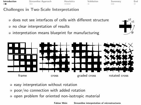
Challenges in Two-Scale Interpretation

does not see interfaces of cells with different structure

no clear interpretation of results

interpretation means blueprint for manufacturing

s2s1

frame cross graded cross rotated cross

easy interpretation without rotation

poor/no connection with added rotation

open problem for oriented non-isotropic material

Fabian Wein Streamline interpretation of microstructures

Introduction Streamline Approach Heuristics Validation Summary End

Streamline Approach

find streamlines based on starting points

similar to Euler’s method solving an ODE:

xn+1 = xn + `cosθ

yn+1 = yn + `sinθ

θ field

start forwardbackward

Fabian Wein Streamline interpretation of microstructures

Introduction Streamline Approach Heuristics Validation Summary End

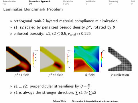
Laminates Benchmark Problem

orthogonal rank-2 layered material compliance minimization

s1, s2 scaled by penalized pseudo density ρp, rotated by θ

enforced porosity: s1,s2≤ 0.5,vtotal ≈ 0.225

ρp s1 field ρp s2 field θ field visualization

s1⊥ s2: perpendicular streamlines by θ + π

2

s1 is always the stronger direction, ∑s1� ∑s2

Fabian Wein Streamline interpretation of microstructures

Introduction Streamline Approach Heuristics Validation Summary End

Applying the Streamline Approach

color coding: given parameter and calculated parameterstart streamlines for s1 and s2 in every cell center

(a) c = 1→ vtotal = 0.89 (b) c = 0.001→ vtotal = 0.82 (c) c s ≥ smin | vtotal = 0.25

(a) streamlines tend to overlap to dense bundles → undesired solid(b) minimal drawn line thickness is one pixel → too heavy void(c) → define minimal line stiffness smin, find scaling c to satisfy vtotal

Fabian Wein Streamline interpretation of microstructures

Introduction Streamline Approach Heuristics Validation Summary End

Indirect Control of Line Thickness

many lines force strong downscaling to meet volume → thin linesevaluate data on virtual grid hs , here 20×20

Algorithm to reduce number of lines

start line in virtual cell only with tmax lines → sort lines!

still arbitrary many lines can traverse virtual cells

tmax = ∞→ c = 0.0011 tmax = 5→ c = 0.015 tmax = 1→ c = 0.32Fabian Wein Streamline interpretation of microstructures

Introduction Streamline Approach Heuristics Validation Summary End

Increasing Minimal Line Thickness

s1� s2 in given example → s2 only expressed by thin lines

assume we do not want too thin lines for manufacturing

too restrictive minimal thickness smin eliminates s2

→ separate virtual grid spacing hs1 and hs2

hs1,hs2 = 40,smin = 0.05 hs1,hs2 = 40,smin = 0.2 hs1 = 40,hs2 = 10,smin = 0.2

Fabian Wein Streamline interpretation of microstructures

Introduction Streamline Approach Heuristics Validation Summary End

Increasing Minimal Line Thickness - Displacements

(a) hs1,hs2 = 40,smin = 0.05

(b) hs1,hs2 = 40,smin = 0.2

(c) hs1 = 40,hs2 = 10,smin = 0.2

albeit ∑s2� ∑s1 it is essential to have s2!

(a) u>f =0.14, vis u×20 (b) u>f =0.94 (c) u>f =0.16, vis u×20

Fabian Wein Streamline interpretation of microstructures

Introduction Streamline Approach Heuristics Validation Summary End

Numerical Validation - Parameter Study

vary hs2 ∈ [10,40] and smin ∈ [0.01,0.2] → image → mesh → FEM

fixed hs1 = 40 and tmax = 2

1020

3040

0.0

0.1

0.20.210

0.215

0.220

0.225

0.230

vtotal

hs2

smin

vtotal

1020

3040

0.0

0.1

0.2

1.02.03.04.05.0 u

T f

hs2

smin

uT f

minimal too low: many thin lines → vtotal cannot be reached

minimal too high: loose information → poor compliance

u>f : homogenized=1.51, streamline ≈ 1.55 . . . 2.0, SIMP=1.13

Fabian Wein Streamline interpretation of microstructures

Introduction Streamline Approach Heuristics Validation Summary End

Summary

Pros

the streamline approach can interpret oriented 2D two-scale results!

performance of interpretation is “close” to homogenized performance

full control of local line thickness

correct orientation of lines (including relative angle)

Cons

poor control of local line density/ local porosity

interpretation is relatively far away from optimized design

problem specific hand tuned heuristics (hs1, hs2, smin, tmax, c)

Fabian Wein Streamline interpretation of microstructures

Introduction Streamline Approach Heuristics Validation Summary End

Outlook

remove dead line ends and not connected line segments

identify effects of streamline and optimization parameters

go to 3D!

minor details extend to 3D 3D application

Fabian Wein Streamline interpretation of microstructures

Introduction Streamline Approach Heuristics Validation Summary End

thank you for your attention!

Fabian Wein Streamline interpretation of microstructures

Introduction Streamline Approach Heuristics Validation Summary End

Hard Shell

nature has hard shell outside → not in optimization

streamlines tend to cluster at boundaries → why?

strong boundary might be out of load point!

wikipedia

direct visualization start streams at max values force streams at load

Fabian Wein Streamline interpretation of microstructures

Introduction Streamline Approach Heuristics Validation Summary End

Impact of Macroscopic Optimization Regularization

optimization with different regularization for s1,s2 and θ

(a) low regularization (b) med regularization (c) strong regularization

u>f (hom/eval): (a) (1.36/1.51), (b) (1.40,1.50), (c) (1.51,1.66)

apparently streamline have own regularization (hs1 = 40,hs2 = 10)

Fabian Wein Streamline interpretation of microstructures