interpreting communities based on the evolution of a

ORIGINAL ARTICLE

Interpreting communities based on the evolution of a dynamicattributed network

Gunce Keziban Orman1• Vincent Labatut2

• Marc Plantevit3• Jean-Francois Boulicaut4

Received: 22 December 2014 / Revised: 13 May 2015 / Accepted: 18 May 2015

� Springer-Verlag Wien 2015

Abstract Many methods have been proposed to detect

communities, not only in plain, but also in attributed, di-

rected, or even dynamic complex networks. From the

modeling point of view, to be of some utility, the com-

munity structure must be characterized relatively to the

properties of the studied system. However, most of the

existing works focus on the detection of communities, and

only very few try to tackle this interpretation problem.

Moreover, the existing approaches are limited either by the

type of data they handle or by the nature of the results they

output. In this work, we see the interpretation of commu-

nities as a problem independent from the detection process,

consisting in identifying the most characteristic features of

communities. We give a formal definition of this problem

and propose a method to solve it. To this aim, we first

define a sequence-based representation of networks, com-

bining temporal information, community structure, topo-

logical measures, and nodal attributes. We then describe

how to identify the most emerging sequential patterns of

this dataset and use them to characterize the communities.

We study the performance of our method on artificially

generated dynamic attributed networks. We also em-

pirically validate our framework on real-world systems: a

DBLP network of scientific collaborations, and a LastFM

network of social and musical interactions.

Keywords Dynamic attributed networks � Community

interpretation � Topological measures � Emerging sequence

mining

1 Introduction

Complex networks have become very popular as a mod-

eling tool during the last decade because they help to better

understand the intrinsic laws and dynamics of complex

systems. A typical plain network contains only nodes and

links between them, but it is possible to enrich it with

different types of data: link orientation and/or weight,

temporal dimension, attributes describing the nodes or

links, etc. This flexibility allowed to use complex networks

to study real-world systems in many fields: sociology,

physics, genetics, computer science, etc. Newman (2003).

The complex nature of the modeled systems leads to the

presence of non-trivial topological properties in the corre-

sponding networks. Among them, the community structure

is one of the most studied. The notion of community

originally comes from social sciences. It traditionally refers

to groups of persons sharing a common territory (neighbor-

hood, town, city, etc.) or having common relationships

(human relationship, family, etc.) Gusfield (1975). More

recently, it has been used to point out at groups of persons

sharing emotions, having a feeling of belonging together

& Gunce Keziban Orman

[email protected]

Vincent Labatut

[email protected]

Marc Plantevit

[email protected]

Jean-Francois Boulicaut

[email protected]

1 Department of Computer Engineering, Galatasaray

University, Istanbul, Turkey

2 Laboratoire Informatique d’Avignon, Universite d’Avignon,

Avignon, France

3 Universite Lyon 1, CNRS, LIRIS, Villeurbanne 69622,

France

4 INSA-Lyon, CNRS, LIRIS, Villeurbanne 69621, France

123

Soc. Netw. Anal. Min. (2015) 5:20

DOI 10.1007/s13278-015-0262-4

http://crossmark.crossref.org/dialog/?doi=10.1007/s13278-015-0262-4&domain=pdf

http://crossmark.crossref.org/dialog/?doi=10.1007/s13278-015-0262-4&domain=pdf

McMillan and Chavis (1986). In network science, a com-

munity roughly corresponds to a group of nodes more

densely interconnected, relatively to the rest of the network

Fortunato (2010). The community structure of a network

denotes to the way its communities are interconnected. Such

a structure has been observed in many real-world networks

Newman (2003), and it was shown to be directly related to

the way the modeled systems work Fortunato (2010). It is

therefore widely studied, for many objectives: discovering

functionally related objects, studying interactions between

modules, inferring missing attribute values and predicting

unobserved connections, etc. Yang et al. (2013). The ap-

plications are numerous, such as recommendation systems

Chen et al. (2014), viralmarketingLeskovec et al. (2007), or

sentiment analysis Parau et al. (2013).

Because of this popularity, hundreds of different algo-

rithms were developed for community detection Fortunato

(2010).Although thesemethods differ in terms of nature of the

detected communities, type of network they handle, technique

of detection, algorithmic complexity, result quality, and other

aspects, their output can always be basically described as a list

of node groups. More specifically, in the case of mutually

exclusive communities, it is a partition of the set of nodes.

Fromanapplicative point of view, the question is then tomake

sense of these groups relatively to the studied system. In other

words, for the community structure to be useful, it is necessary

to interpret the detected communities. This problem is ex-

tremely important from the end user’s perspective. And yet,

almost all works in the field of community detection concern

the definitionofdetection tools and their evaluation in termsof

performance Fortunato and Lancichinetti (2009). Few re-

searchers have addressed the problem of characterizing and

interpreting the communities (Tumminello et al. 2011; La-

batut and Balasque 2012; Labatut and Balasque 2013; Yang

et al. 2013). The existing methods suffer from various

limitations: some are subjective, others focus on nodal at-

tributes only, or on topological properties only, or mix these

data in anunclearway, asweexplain inmoredetails inSect. 2.

Moreover, in most of these works, the problem of community

interpretation is not defined as a problem in itself.

In this work, we consider the interpretation problem as

independent from the approach used for community detec-

tion. We break it down to two separate sub-problems: on the

one hand, representing a community in an appropriate way,

and on the other hand, finding the most characteristic ele-

ments from this representation. To solve them,we propose an

approach based on the original definition of the notion of

community in social sciences, which underlines that nodes

belonging to the same community should be relatively

similar and/or share a common behavior. Assessing node

similarity requires describing nodes, which can be per-

formed both in terms of individual information (i.e., personal

characteristics) and relational information (i.e., connection

to the rest of the network). Concretely, the former corre-

sponds to nodal attributes, whereas the latter depends on the

network topology. The behavior of a node can be described

in terms of evolution of its individual and relational infor-

mation. To take these three aspects (individual, relational,

temporal) into account, we need to work with dynamic at-

tributed networks, i.e., time evolving networks whose nodes

are describedwith various fields. To summarize, our aimwas

to detect common changes in topological features and at-

tribute values over time periods, in dynamic attributed net-

works. More precisely, we aim at finding the most

characteristic sequential patterns for each community. These

represent the general trends for the community and provide a

support for its interpretation.

Our first contribution is to formalize community inter-

pretation as a specific problem, distinct from community

detection. In particular, it should be independent from the

method used to detect communities, rely on an easily

replicable systematic approach, and be as automated as

possible. Our second contribution is the definition of a

method taking advantage of a sequential representation of

networks, in order to extract characteristic patterns allow-

ing the interpretation of communities. Our third contribu-

tion is to evaluate our method on both artificially generated

and real-world networks. To this aim, we propose an ex-

tension of an existing generative model Greene et al.

(2010), in order to produce attributed dynamic networks.

The real-world data are an existing co-authorship network

coming from DBLP Desmier et al. (2012) and a network of

Jazz listeners we extracted from LastFM.

The rest of this article is organized as follows. In

Sect. 2, we review and comment in more details the ex-

isting works more or less directly related to community

interpretation. Then, in Sect. 3, first we introduce some

necessary concepts related to networks analysis and se-

quential pattern mining. Second, we give a formal de-

scription of the community interpretation problem we

handle. In the following part, in Sect. 4, we give a general

description of the approach we propose for community

interpretation and illustrate it on a small toy network. Our

method for community interpretation is then described in

details in Sect. 5. In Sects. 6 and 7, we present our results

obtained on artificial and real-world networks, respective-

ly. Finally, we conclude in Sect. 8 by summarizing our

work and explaining how it can be extended.

2 Related work

Authors historically interpreted the communities they found

in an ad hoc way (Girvan and Newman 2002; Rosvall and

Bergstrom 2008; Blondel et al. 2008), but this somewhat

subjective approach does not scale well on large networks.

20 of 22 Soc. Netw. Anal. Min. (2015) 5:20

123

More recently, several authors used topological mea-

sures to characterize community structures in plain net-

works. Lancichinetti et al. (2010), visually examined the

distribution of some community-based topological mea-

sures, both at local and intermediary levels. Their goal was

to understand the general shape of communities belonging

to networks modeling various types of real-world systems.

Leskovec et al. (2008) proposed to study the community

structure as a whole, by considering it at various scales,

thanks to a global measure called conductance. These two

studies are valuable; however, from the interpretation

perspective, they are limited by the fact they consider the

network as a whole. Communities are studied and char-

acterized collectively, in order to identify trends in the

whole network, or even a collection of networks.

In order to characterize each community individually,

some authors took advantage of the information conveyed by

nodal attributes, when they are available. Tumminello et al.

(2011) proposed a statistical method to characterize the

communities in terms of the over-expressed attributes found

in the elements of the community. Labatut and Balasque

(2012) interpreted the communities of a social attributed

network. They used statistical regression and discriminant

correspondence analysis to identify the most characteristic

attributes of each community. Both studies are valuable;

however, they do not take advantage of the available topo-

logical measures to enhance the interpretation process.

Certain community detection methods take advantage of

both relational (structure) and individual (attributes) in-

formation to detect communities. It seems natural to pro-

duce the results that the output can be used for

interpretation purposes. For example, Zhou et al. (2009)

interpreted the communities in terms of the attributes used

during the detection process, and Yang et al. (2013) iden-

tified the top attributes for each identified community.

However, the problem with these community detection-

based methods is that the notion of community is often

defined procedurally, i.e., simply as the output of the de-

tection method, without any further formalization. It is

consequently not clear how structure and attributes affect

the detection and hence the interpretation process. All these

methods additionally rely on the implicit assumption of

community homophily. In other words, communities are

supposed to be groups of nodes both densely intercon-

nected and similar in terms of attributes. To our knowl-

edge, no study has ever shown that this feature was present

in all systems or even in all the communities of a given

network or that all attributes were concerned. It is therefore

doubtful that those methods are general enough to be ap-

plied to any type of network.

Another method was recently defined based on frequent

pattern mining, which can be used for community inter-

pretation. Stattner and Collard (2012) introduced the notion

of frequent conceptual link. A conceptual link corresponds

to a set of links from the original network, connecting

nodes who share similar attributes. Such a link is said to be

frequent when the number of links it represents is above a

given threshold. This method can be seen as a general-

ization of the notion of homophily and was initially used to

simplify the network and help understanding it. Finding

frequent conceptual links amounts to detecting groups of

nodes sharing common attributes, with a pattern mining

point of view. This method considers both the network

structure and the nodal attributes; however, it ignores their

evolution, i.e., it does not take the temporal aspect into

account.

3 Definitions and problem statement

In this section, we first introduce some concepts used in the

rest of the article. We then state formally the problem of

community interpretation.

3.1 Preliminary definitions

We first define several concepts related to community

structures and complex networks in general. In particular,

we describe a selection of topological measures later used

in the experimental sections. In the second part, we focus

on concepts related to sequential pattern mining.

3.1.1 Network-related concepts

We formally define a dynamic attributed network as

G ¼ hG1; . . .;Ghi, i.e., a sequence of chronologically

ordered graphs Gt (1� t� h), which we call time slices. A

time slice Gt ¼ ðV;Et;AÞ is a triple such that V is the set of

nodes, Et � V � V is the set of links, and A is the set of

node attributes. The nodes are the same for all time slices,

and we can consequently note j V j ¼ n the size of each

time slice, as well as the dynamic network. The set of nodal

attributes is the same for all time slices, but the values

associated to the nodes can change.

An evolving community structure of a dynamic at-

tributed network G is a sequence hC1; . . .;Chi of chrono-

logically ordered community structures Ct (1� t� h),where each Ct corresponds to a community structure of Gt.

A community structure Ct ¼ fC1t ; . . .;C

ktt g is itself a par-

tition of the node set, whose parts Cct (1� c� kt) are the

communities. We note CtðvÞ the function associating a

node v to its community in Ct. The size of a given com-

munity Cct is its number of nodes jCc

t j. It is important to

note that, due to the fact communities might split, merge,

or disappear, communities represented by the same index c

Soc. Netw. Anal. Min. (2015) 5:20 of 22 20

123

in two different time slices do not necessarily match. For

instance, communities C14 (first community at t = 4) and

C110 (first community at t = 10) might be completely

different.

A topological measure quantifies the structural properties

of the network or its components. Here, we focus on nine

nodal measures very well known in the community of social

networks analysis: for this reason, we present them very

briefly. Each one will be processed for each node, at each

time slice. The simplest, the degree, is the number of links

attached to a node. The local transitivityWatts and Strogatz

(1998) of a node corresponds to the ratio of the number of

links present between its neighbors to themaximum possible

number of such links. The eccentricity of a node is its furthest

(geodesic) distance to any other node in the network Harary

(1969). The betweenness centrality measures how much a

node lies on the shortest paths connecting other nodes; it can

be considered as a measure of accessibility Freeman (1979).

The closeness centrality quantifies how near a node is to the

rest of the network, in average Sabidussi (1966). The Ei-

genvector centrality measures the influence of a node in the

network based on its spectral properties. It is proportional to

the sum of the centrality of the node neighbors Bonacich

(1987). The within module degree and participation coeffi-

cient are two measures proposed by Guimera and Amaral

(2005) to characterize the community role of nodes. The

within module degree is defined as the z-score of the internal

degree, i.e., the number of neighbors a node has in its own

community. The participation coefficient characterizes how

heterogeneously the neighbors of a node are distributed

among communities. It gets close to 1 if all the neighbors are

uniformly distributed among all the communities, and 0 if

they are all gathered in the same community. The embed-

dedness represents the proportion of neighbors of a node

belonging to its own community Lancichinetti et al. (2010).

Unlike the within module degree, the embeddedness is

normalized with respect to the node and not the community.

3.1.2 Pattern-related concepts

A node descriptor is either a topological measure or a node

attribute from A. Let D ¼ fD1;D2; . . .;Dkg be the set of all

descriptors. Each descriptor from D can take one of several

discrete values, defined in its domainDi (1� i� k). All our

topological measures are real-valued, so we have to dis-

cretize them to fit this definition. Moreover, the same ap-

plies to real-valued attributes. The details of the

discretization and binning processes are explained in

Sect. 5.1.2.

An item li ¼ ðDi; xÞ 2 D�Di is a couple constituted of

a descriptor Di and a value x from its domain Di. The set of

all items is noted I. An itemset h is any subset of I.

Although itemsets are sets, in the rest of this article, we

represent them between parentheses, e.g., h ¼ ðl1; l3; l4Þbecause it is the standard notation in the literature.

A sequence s ¼ hh1; . . .; hmi is a chronologically

ordered list of itemsets. Two itemsets can be consecutive in

the sequence while not correspond to consecutive time

slices: the important point is that the first to appear must be

associated to a time slice preceding that of the second one.

In other words, hi occurs before hiþ1 and after hi�1. The

size of a sequence is the number of itemsets it contains.

A sequence a ¼ ha1; . . .; ali is a sub-sequence of an-

other sequence b ¼ hb1; . . .; bmi iff 9i1; i2; . . .; il such that

1� i1\i2\ � � �\il � m and a1 � bi1 ; a2 � bi2 ; . . .; al �bil . This is noted aYb. It is also said that b is a super-

sequence of a,which is noted b w a.The node sequence u(v) of a node v is a specific type of

sequence of size h (i.e., the number of time slices). We

have uðvÞ ¼ hðl11; . . .; lk1Þ. . .ðl1h; . . .; lkhÞi, where lit is the

item containing the value of descriptor Di for v at time t. A

node sequence u(v) includes h itemsets, i.e., it represents all

time slices. Each one of these itemsets contains all k de-

scriptor values for the considered node at the considered

time. In other words, u(v) contains all the available de-

scriptor-related data for node v.

We build the enlarged node sequence uenlðvÞ of a node vby adding a community-related item to each itemset of its

node sequence: uenlðvÞ ¼ hðl11; . . .; lk1;C1ðvÞÞ. . .ðl1h; . . .;lkh;ChðvÞÞi. The sequence database M can then be obtained

by collecting the enlarged node sequences uenlðvÞ of all

nodes in the considered network.

The set of supporting nodes SðsÞ of a sequence s is

defined as SðsÞ ¼ fv 2 V : uðvÞ w sg. The support of a

sequence s; SupðsÞ ¼ jSðsÞj=n , is the proportion of nodes,

in G, whose node sequences are equal to s or are super-

sequences of s.

The set of supporting nodes of a sequence s relatively to

a node group X is defined as Sðs;XÞ ¼ fv 2 X : uðvÞ w sg.Its support relatively to the same node group,

Supðs;XÞ ¼ jSðs;XÞj=jXj, is the proportion of nodes, in X,

whose node sequences are equal to s or super-sequence of

s. A node group might directly correspond to a community

taken at one time slice or to the nodes belonging to the

same communities over a series of time slices.

The growth rate of a pattern s relatively to a node group

X is Grðs;XÞ ¼ Supðs;XÞ=Supðs;XÞ, where X is the com-

plement of X in V , i.e., X ¼ V n X. The growth rate mea-

sures the emergence of s: a value larger than 1 means s is

particularly frequent (i.e., emerging) in X, when compared

to the rest of the network.

We say a sequence is community related if it contains at

least one community-related item. If all its items are

community related, it is said to be a community sequence,


123

such as hCc1t1 ;C

c2t2 ; . . .;C

cmtm i. On the contrary, we call it

community independent if it contains no community-relat-

ed item at all.

For a community-related sequence s, we define its

community-wise sub-sequence swise as its maximal com-

munity sub-sequence. In other words, it is a sequence

swiseYs such that swise is a community sequence, and there

is no other community sequence s0 fulfilling both condi-

tions s0Ys and swise s0. Similarly, for a community-re-

lated sequence s, we define its community-less sub-

sequence sless as its maximal community-independent sub-

sequence. In other words, it is a sequence slessYs such that

sless is a community-independent sequence, and there is no

other community-independent sequence s0 fulfilling both

conditions s0Ys and sless s0.Given a minimum support threshold noted minsup, a

frequent sequential pattern (FS) is a sequence whose

support is greater or equal to minsup. A closed frequent

sequential pattern (CFS) is a FS which has no super-se-

quence possessing the same support.

3.2 Problem statement

We see the problem of community interpretation as the

operation consisting in identifying the most characteristic

features of certain groups of nodes. But what is a feature?

And how can we know if it is a characteristic one? To be

able to solve the interpretation problem, we need first to

answer these two questions. In other words, our problem of

interest can be broken down to two sub-problems:

1. Finding an appropriate way to represent a community;

2. Defining an objective method to decide which parts of

this representation are characteristic.

In this section, we consider separately these two sub-

problems and formalize them.

3.2.1 Appropriate community representation

It is obviously not possible to know in advance which

pieces of the information describing the considered com-

munity will be the most characteristic. Therefore, we need

to be able to represent all the available information, in a

computationally efficient way. A community can be de-

scribed only in terms of its constituting elements, since it is

by definition a set, so its representation must be defined at

the nodal level. It is necessary to use a representation able

to handle node similarity, interconnection, and co-evolu-

tion. More formally, this means a community must be

represented through its nodal attributes, topological prop-

erties, and temporal evolution. The attributes correspond to

the individual characteristic of the objects composing the

modeled social system, the topological properties describe

how these objects interact, and the temporal evolution is

the consequence of the system dynamics.

In the context of community interpretation, the

problem of finding an appropriate community rep-

resentation, for a dynamic attributed network and its

community structure, is equivalent to that of encoding

all information describing the evolution of each node

from each community. This encoding should be

compact enough to avoid redundancies, but complete

enough to describe the evolution of the community.

To fulfill these constraints, we propose to represent each

node using the sequence of its attributes and topological

measures, taken at different discrete times of the system

evolution. To our knowledge, such a sequential represen-

tation was never used for networks before. We could use

the database M described in the previous section, which is

the collection of enlarged node sequences uenlðvÞ (8v 2 V).

However, this representation would not be very compact

because several nodes could be described (totally or

partially) by similar sequences. To avoid this, we instead

represent a community through the sequential patterns

present among the sequences describing the nodes it

contains.

For a node v, we note Pv the set of all possible sub-

sequences of its enlarged node sequence, i.e.,

Pv ¼ fsYuenlðvÞg. Let P be the union of all the Pv over all

nodes, i.e., P ¼S

v2V Pv, and B be the subset of its com-

munity sequences. Let mi denote such a community se-

quence and l be the cardinality of B, then we have

B ¼ fm1; . . .;mlg. We state that the problem of community

representation is finding a set C ¼ fc1; . . .; clg such that

ci ¼ fs 2 P : s w mig with 1� i� l. In other words, for

each community sequence mi found in the database, we

want to identify the set ci of all its super-sequences presentin the same database. Those, by definition, are themselves

community-related sequences.

The set C includes all the necessary information related

to each community sequence. It represents the sub-se-

quences common to more than one node only once and

therefore eliminates the redundancies. Consequently, it

fulfills our requirements of being both a complete and

compact representation.

3.2.2 Identifying characteristic features

Let us now turn to the second problem: finding, in an

objective way, which parts of the community description

are characteristic. The criteria used to identify this rele-

vance must be compatible with our representation of a

community, which takes the form of sets of sequential

patterns.


123

In the context of community interpretation, the

problem of identifying characteristic features among

the sequences representing a community consists in

selecting some objective criteria to assess the rep-

resentative power of these sequences, and a method

to select the most representative ones.

The representation defined in the previous section takes the

form of a set C ¼ fc1; . . .; clg, where each ci represents theset of community-related super-sequences of a community

sequence mi (as of the considered database). We define one

condition and two criteria for a member of ci to be

characteristic of mi. The condition is that it must be

informative. We consider a sequence to be informative if it

is closed Gallo et al. (2007), i.e., if it does not have any

super-sequence with the same support or a better one. The

two criteria are that the sequence must be both prevalent

and distinctive. We measure the prevalence of a sequence s

in ci with its support Supðs; SðmiÞÞ, where SðmiÞ is the

supporting node set of the reference community sequence

mi (i.e., the groups of nodes following the sequence). We

measure the distinctiveness through the growth rate

Grðs; SðmiÞÞ Dong and Li (1999).

Then, the problem of identifying the characteristic fea-

tures of a community sequence mi consists in selecting a

subset c0i � ci such that c

0i ¼ fs 2 ci : s is closed ^ Supðs;

SðmiÞÞ�minsup ^ Grðs; SðmiÞÞ�mingrg, where minsup and

mingr are lower thresholds for the support and growth rate,

respectively. We note C0 ¼ fc0

1; . . .; c0lg the set containing

the characteristic patterns of each community sequence in

the network.

4 Overview of our evolution-based approach

Our approach is based on the representation of dynamic at-

tributed networks under the form of sequences. One se-

quence represents a node and its behavior: it contains the

topological, attribute, and community-related information

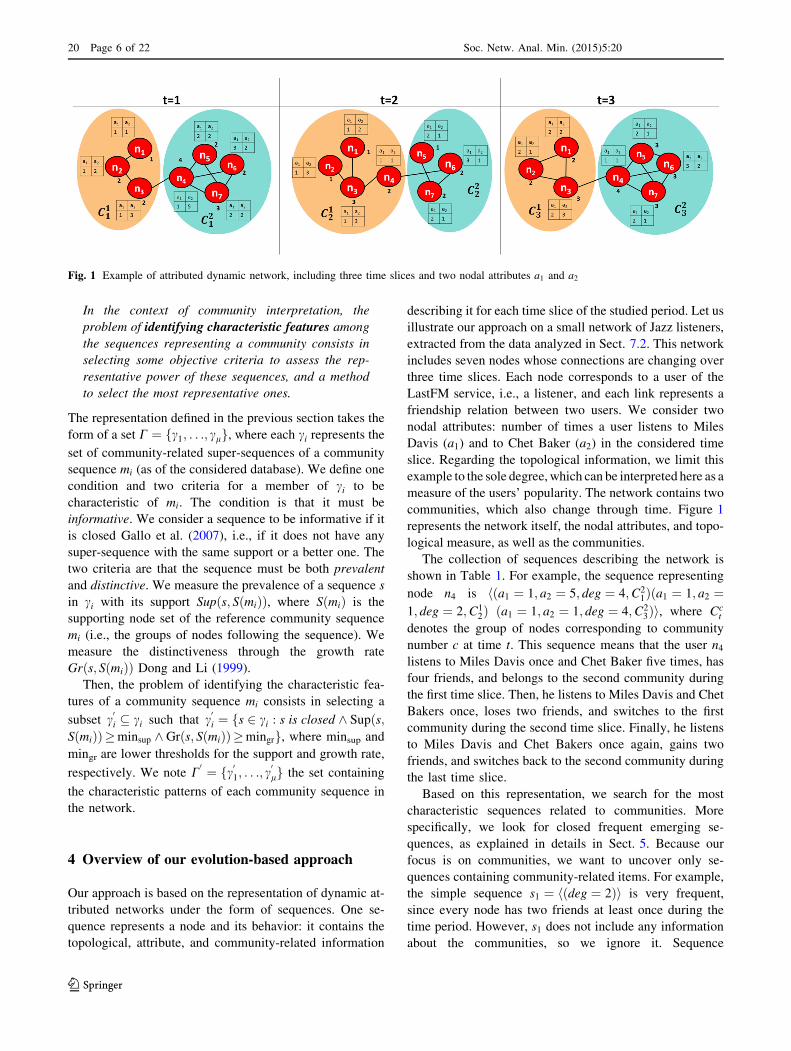
describing it for each time slice of the studied period. Let us

illustrate our approach on a small network of Jazz listeners,

extracted from the data analyzed in Sect. 7.2. This network

includes seven nodes whose connections are changing over

three time slices. Each node corresponds to a user of the

LastFM service, i.e., a listener, and each link represents a

friendship relation between two users. We consider two

nodal attributes: number of times a user listens to Miles

Davis (a1) and to Chet Baker (a2) in the considered time

slice. Regarding the topological information, we limit this

example to the sole degree, which can be interpreted here as a

measure of the users’ popularity. The network contains two

communities, which also change through time. Figure 1

represents the network itself, the nodal attributes, and topo-

logical measure, as well as the communities.

The collection of sequences describing the network is

shown in Table 1. For example, the sequence representing

node n4 is hða1 ¼ 1; a2 ¼ 5; deg ¼ 4;C21Þða1 ¼ 1; a2 ¼

1; deg ¼ 2;C12Þ ða1 ¼ 1; a2 ¼ 1; deg ¼ 4;C2

3Þi, where Cct

denotes the group of nodes corresponding to community

number c at time t. This sequence means that the user n4listens to Miles Davis once and Chet Baker five times, has

four friends, and belongs to the second community during

the first time slice. Then, he listens to Miles Davis and Chet

Bakers once, loses two friends, and switches to the first

community during the second time slice. Finally, he listens

to Miles Davis and Chet Bakers once again, gains two

friends, and switches back to the second community during

the last time slice.

Based on this representation, we search for the most

characteristic sequences related to communities. More

specifically, we look for closed frequent emerging se-

quences, as explained in details in Sect. 5. Because our

focus is on communities, we want to uncover only se-

quences containing community-related items. For example,

the simple sequence s1 ¼ hðdeg ¼ 2Þi is very frequent,

since every node has two friends at least once during the

time period. However, s1 does not include any information

about the communities, so we ignore it. Sequence

Fig. 1 Example of attributed dynamic network, including three time slices and two nodal attributes a1 and a2


123

s2 ¼ hða1 ¼ 1;C11Þða1 ¼ 1;C1

2Þða1 ¼ 2;C13Þi, on the con-

trary, is a bit less frequent (supported by the first three

nodes) but contains community information. It can be in-

terpreted as a trend regarding the listening habits of certain

nodes of the first community.

At this point, it is important to understand that a com-

munity is not necessarily a stable group of nodes. On the

contrary, it can undergo rather dramatic changes during its

evolution: merge, split, complete disappearance, etc. To

handle this case, it is necessary to focus the interpretation

process on groups of nodes going through several times

slices together while possibly switching communities si-

multaneously. For this purpose, we separate sequences such

as s2 in two sub-sequences: on the one hand, a community

sequence hðC11ÞðC1

2ÞðC13Þi containing exclusively commu-

nity-related items and used to represent how the concerned

nodes evolve community-wise , and on the other hand, a

characteristic sequence hða1 ¼ 1Þða1 ¼ 1Þða1 ¼ 2Þi con-

taining no community-related items at all, which serves as

a basis to interpret this group of nodes. This is better il-

lustrated when considering the second community: the

community pattern hðC21ÞðC2

3Þi allows covering nodes n4 to

n7, whereas adding ðC22Þ would exclude n4.

Our last point concerns the covering of the community

sequences. For hðC11ÞðC1

2ÞðC13Þi, we identified s2, which de-

scribes all three concerned nodes. However, it is not always

possible to do so: it is noticeably the case for hðC21ÞðC2

3Þi. Forthis community sequence, the best characteristic sequence is

s3 ¼ hða1 ¼ 2Þða1 ¼ 2; a2 ¼ 1Þða1 ¼ 2; a2 ¼ 1; deg ¼ 3Þi,which is supported only by n5 and n7 but not n4 and n6. In this

situation, we identify supplementary sequences such as s4 ¼hða2 ¼ 1; deg ¼ 2Þi to improve the coverage and use them to

complement the interpretation.

5 Proposed method

Our problem definition requires us to search for informa-

tive, prevalent, and distinctive sequences by taking ad-

vantage of a compact and complete representation of

dynamic attributed networks. To fulfill this goal, we

propose a two-stepped approach. In the first, we build a

sequence database, in order to represent a dynamic at-

tributed network. The second then consists in searching for

meaningful sequences while respecting the constraints de-

fined in Sect. 3.2.2.

5.1 Creating the sequence database

As explained in Sect. 3.1.1, a sequence database is the

collection of enlarged node sequences uenlðvÞ for all nodesin the network. Creating this database thus requires first

calculating the topological measures and identifying the

communities. Moreover, all real-valued nodal descriptors

must be discretized to allow sequential pattern mining.

Data preparation may also include some additional pre-

processing, such as the binning of discrete descriptors or

the combination of topological measures, in order to im-

prove the readability of the obtained patterns, or to lighten

the computational load.

5.1.1 Community detection

An important idea with our approach is to interpret the com-

munities independently from the method used for their de-

tection. But of course, we need a reference community

structure to work with. Community detection for time

evolving networks is much less developed than for static

networks. Moreover, it was shown Aynaud and Guillaume

(2010) that applying static community detection methods on

evolving networks does not lead to stable results,which shows

there are non-negligible differences between these two prob-

lems.Note that our goal herewas not to perform an exhaustive

comparison of algorithms able to process dynamic networks:

the focus of this article is not community detection itself, but

rather the interpretation of the detected communities.

Orman (2014), the author tested four different versions

of the Louvain algorithm Blondel et al. (2008), modified

for dynamic networks. She has shown that Incremental

Louvain Aynaud and Guillaume (2010) was generally

above the others in terms of performance. So, on the basis

of this study, we selected this algorithm to detect evolving

Table 1 Node sequences

representing the network from

Fig. 1

ID Related sequence

n1 hða1 ¼ 1; a2 ¼ 1; deg ¼ 1;C11Þða1 ¼ 1; a2 ¼ 2; deg ¼ 1;C1

2Þða1 ¼ 2; a2 ¼ 2; deg ¼ 2;C13Þi


2Þða1 ¼ 2; a2 ¼ 1; deg ¼ 2;C13Þi


2Þða1 ¼ 2; a2 ¼ 3; deg ¼ 3;C13Þi


2Þða1 ¼ 1; a2 ¼ 1; deg ¼ 4;C23Þi


2Þða1 ¼ 2; a2 ¼ 1; deg ¼ 3;C23Þi


2Þða1 ¼ 3; a2 ¼ 2; deg ¼ 3;C23Þi


2Þða1 ¼ 2; a2 ¼ 1; deg ¼ 3;C23Þi


123

communities in our own data. Unlike other variants of

Louvain, Incremental Louvain takes into account the pre-

vious communities when processing a time slice, which

results in some temporal smoothing. For the first time slice,

the original version of Louvain is applied. Then, for the

next time slices, the algorithm starts with the community

structure found at the previous time slice (rather than

putting each node in its own community) and then goes on

with the original processing [greedy optimization of the

modularity measure, see Blondel et al. (2008)]. The time

complexity of this method is in Oðn log nÞ Blondel (2011)for one time slice when the network is sparse. In our case, it

is applied on h time slices, so the total complexity is in

Oðhn log nÞ.

5.1.2 Data preparation

As explained in Sect. 3.1.2, the descriptors used to fill our

sequence database are either nodal attributes or topological

measures. All the measures we selected are numerical,

whereas the attributes can be of any data type, including

categorical and numerical values. However, it is not pos-

sible to directly use real values as items for sequential

pattern mining because this method handles only discrete

data. So, it is necessary to first discretize this type of de-

scriptor. Moreover, even for integer descriptors, it can be

interesting to bin their domains for several reasons. First,

having too many distinct values in the domain of a de-

scriptor tends to significantly increase the number of de-

tected patterns while decreasing their support, thereby

preventing to uncover results which would be sufficiently

general to be informative. Second, due to the increase in

the number of patterns, both processing time and memory

occupation also significantly increase during pattern min-

ing (as shown in Sect. 6). Three, the meanings of two

distinct descriptor values can be close enough that they can

be considered as similar without any significant informa-

tion loss.

Whatever the preparation method (discretizing or bin-

ning), it is necessary to define thresholds. This can be done

either by taking advantage of some expertise regarding the

system or measures or using an automatic approach, for

instance through the identification of denser zones in the

considered attribute domain. A clustering algorithm can

fulfill this goal, with the added advantage of being able to

handle simultaneously several descriptors. Indeed, for

computational reasons, as well as to ease human interpre-

tation, it can be relevant to go beyond discretization and

binning and to combine several descriptors into one. This

approach was previously applied, in the context of social

networks analysis, to some variants of Guimera & Amar-

al’s measures, in order to identify community roles Dugue

et al. (2014).

We propose to generalize this idea to the preparation of

all the topological measures we use in this work

(Sect. 3.1.1). We first distinguish three groups of the-

matically related measures: centrality related (eccentricity,

betweenness, closeness, Eigenvector), community related

(embeddedness, within module degree, participation co-

efficient), and local (degree, local transitivity). The first

group concerns the position of the node in the whole

network, the second focuses on the community structure,

and the third represents its local connectivity. Each group

is clustered separately using the k-means algorithm, which

was chosen because it is a well-known and fast method.

The number of clusters (parameter k) is decided by op-

timizing the average Silhouette width Rousseeuw (1987),

a widespread cluster quality measure whose interpretation

is clearly defined. After this process, our set of nine

topological measures is replaced by three discrete de-

scriptors, whose values correspond to the detected

clusters.

5.2 Mining the sequence database

The first step of our mining process consists in identifying

all CFS, relatively to the support threshold minsup. Among

them, the most distinctive ones are selected using the

growth rate threshold mingr. Finally, an additional filtering

is performed to only keep the sequences necessary for a

good coverage of the considered communities. This section

is dedicated to the description of these three steps.

Table 2 Values of the attribute-related parameters for each experiment

Model parameters Experiment 1 Experiment 2 Experiment 3

Number of attributes f1; 3; 5g f3g f3gValues of attributes ½0; 9� ½0; 9� ½0; 9�Distribution type fdegenerateg fdegenerateg fdegenerate;binomial; uniform;powergEvolution percentage f0g f5; 20; 50; 100g f5gAim Descriptor number Descriptor stability Descriptor homogeneity

Bold values at each experiment column signify the changing values of related parameters whereas the other parameter values stay constant


123

5.2.1 Mining the closed frequent sequences

We use Closed Sequential Pattern Mining (CloSpan) Yan

et al. (2003) to mine the CFS relatively to our minsupthreshold. It is an efficient algorithm able to identify long

sequences in real-world data, in a practical time. It relies on

the mining strategy introduced in PrefixSpan Pei et al.

(2001).

At first, CloSpan creates a candidate set, which is a

super-set of the closed frequent sequences. These candi-

dates are stored into a so-called prefix sequence lattice.

Second, the non-closed sequences are eliminated. A naıve

approach consists in checking, for all candidate sequences,

if there is any super-sequence with the same support in the

prefix sequence lattice. But it is a costly operation. Thus,

Yan et al. adopted the fast subsumption checking algorithm

introduced Zaki and Hsiao (2002). It is designed to manage

a hash table in which, for each sequence s, the associated

hash key is the sum of the corresponding sequences IDs.

Here, the corresponding sequences of a sequence s refer to

all sequences with prefix s, i.e., the members of its pro-

jected database [c.f. Yan et al. (2003) for the explanation

and formalization of this notion of projected database of a

sequence]. Li et al. (2006), the authors claim that the time

complexity of the last step of CloSpan (pruning prefix se-

quence lattice, the most demanding step) is in Oðn2Þ, wheren is the size of the data (in our case: the number of nodes),

if the maximum length of the frequent sequences is con-

strained by a constant.

5.2.2 Identifying the emerging patterns

The emergence is assessed by processing the growth rates

of the sequences, as described in Algorithm 1. CloSpan

outputs all the CFS related to the considered database, as

well as their support, and these data constitute the input of

our algorithm, together with the database M itself. Each

sequence is processed separately.

The first step consists in determining if the sequence is

relevant. Indeed, CloSpan identifies both the sequences

showing general trends over the whole network (i.e.,

community-independent CFS) and those relative to com-

munity sequences (i.e., community-related CFS). In our

situation, we need to focus only on the latter, so it is

necessary to first separate them from the former. This is

done through the function isCommunityRelated,

whose complexity is in OðhÞ, where h is the size of the

longest possible sequence.

For each remaining CFS s, we apply a parsing procedure

in order to break it down to its community-wise and com-

munity-less sub-sequences, noted swise and sless, respec-

tively. The former is simply the community sequence of

interest, whereas the latter is potentially one of its char-

acteristic sequences. This task is performed by the function

separate, which is also in OðhÞ. Then, swise is added to

B, which gathers all community sequences. We remind the

reader that, according to the definitions from Sect. 3.2.1,

B ¼ fm1; :::;mlg is meant to eventually contain all com-

munity sequences mi.

Next, we want to process the growth rate of sless for the

supporting nodes of swise. To this aim, we need to retrieve

Table 3 Characteristic patterns detected for two DBLP communities

Time

slice

Community

size

Pattern Support Growth

rate

ID

6 120 {high embeddedness}{SDM = 1}{high betweenness, low closeness, high participation coeff.}

{high betweenness, low closeness, high participation coeff.}

40 6.86 1

{high betweenness}{high embeddedness, ICDM = 1} {total conference between 1 and 5} 40 6.00 2

{high embeddedness}{TKDE = 1, total journal between 1 and 5} {high embeddedness, total

journal between 1 and 5} {total journal between 1 and 5}{total journal between 1 and 5}

40 4.00 3

8 113 {ILP = 1} {high betweenness, low closeness, high embeddedness} 40 59.08 4


123

the supports of both these sub-sequences. We use the

function processSup to process the growth rate of a

given sequence s. It first looks s up in the CFS outputted

by CloSpan: if the sequence is closed, then its support is

directly available. Otherwise, it must be processed. This

requires considering each node sequence from the data-

base M (OðnÞ operations in the worst case) and checking

if it is a super-sequence of s (Oðh2Þ operations in the

worst case). The total complexity of the function is

therefore in Oðh2nÞ.Using the supports, the growth rate can be processed in

constant time thanks to the function processGr. It can

then be used to discard non-emerging sequences according

to our mingr threshold. On the contrary, emerging se-

quences are added to C0. We remind the reader that, as

defined in Sect. 3.2.2, C0 ¼ fc01; :::; c

0lg is meant to even-

tually contain all sets c0i, each one gathering all the char-

acteristic sequences associated to community sequence

mi 2 B.

The complexity of the operations contained in the For

loop is in Oðh2nÞ. If we assume CloSpan outputted r CFS,

the total complexity of the whole algorithm is thus in

Oðrh2nÞ.

5.2.3 Selecting the characteristic patterns

The main output of the previous step is C0 ¼ fc0

1; . . .; c0lg.

Each c0i contains community-independent sequences asso-

ciated with the community sequence mi. By construction,

all the sequences in C0 are closed, frequent, and emerging,

and we therefore consider them as characteristic. However,

there can still remain too many of them to perform a

relevant interpretation. As a post-process, we propose an

additional filtering, leading to smaller sets noted C00 ¼

fc00

1; . . .; c00

lg and such that c00

i � c0

i.

We can either consider the sequences with highest

growth rate or with highest support. The complementary

selection procedure we propose is generic and can be ap-

plied to both cases. In the rest of our explanations, we refer

to the criterion of interest (growth rate or support) as the

sequence score. Once the sequence with highest score has

been selected, there is no guarantee for it to cover a suf-

ficient part of the studied community sequence. And in-

deed, in practice, it appears to be the opposite (especially

for the growth rate). It is thus needed to identify other

complementary sequences, allowing us to obtain a more

complete coverage of the nodes supporting the community

sequence.

Intuitively, we want to find a small number of patterns,

such that they cover a significant part of the community

sequence, and are different in terms of supporting nodes.

Or, more formally

– The cardinality ofT

s2c00iSðs;miÞ must be minimal;

– The cardinality ofS

s2c00iSðs;miÞ must be maximal (if

possible: the whole community);

– The cardinality of c00

i must be minimal.

In order to perform this selection, we apply an iterative

procedure described by Algorithm 2. We treat each de-

tected community sequence mi separately. The sequence

set Remaining represents the characteristic sequences

of mi not treated yet, which is why it is initialized with c0i.The node set Covered contains the nodes supporting mi

which are currently also supporting at least one sequence

in c00i , whereas Uncovered contains those who are not.

The following processing is then iterated until those sets

stabilize. First, we apply the function choose, which is

designed to return a sequence s from c00i which was not

used yet and is optimal for our criteria. Its complexity is

in OðnÞ (number of nodes). We then use s to update c00iand the three working sets. At the end of the Repeat

Table 4 Characteristic patterns detected for three LastFM communities

Time

slice

Community

size

Pattern Support Growth

rate

ID

1 105 {Miles Davis between 1 and 5} {high degree, high local transitivity, community non-hub, low

participation coeff.} {high degree, high local transitivity, community non-hub, low

participation coeff. high betweenness, Miles Davis between 1 and 5 }

20 20.36 1

{high degree, high local transitivity, Ella Fitzgerald between 1 and 5, Chet Baker between 1

and 5} {high degree, high local transitivity}

20 8.84 2

1 81 {community non-hub, low participation coeff.} {community non-hub, low participation coeff.}

{Pink Floyd between 5 and 10} {community non-hub, low participation coeff. and The Beatles

between 5 and 10} {community non-hub, low participation coeff.}

15 14.97 3

{The Beatles between 5 and 10}{The Beatles between 5 and 10}{Frank Sinatra between 1 and

5}

15 7.23 4

1 and

4

22 {community non-hub, low participation coeff.} {Pink Floyd between 5 and 10} 15 6.21 5


123

loop, the nodes still uncovered are considered as

anomalies.

The Repeat loop is processed at most maxseq times,

where maxseq is a parameter defined by the user. Indeed,

the goal of this post-processing was to reduce the number

of selected characteristic patterns, so it is necessary to set

a limit corresponding to a subjective acceptable number.

The For loop is repeated exactly l times, so the total

complexity of this algorithm is in OðlnÞ. If we consider

the two first steps of our mining method, we get a final

complexity of Oðn2 þ rh2nþ lnÞ. In practice, CloSpan

detects many more CFS than there are nodes in the net-

work, so r n, and therefore rn n2. The number of

community sequences l is bounded by the total number

of sequences r, so we can neglect the last term. We fi-

nally obtain the following simplified expression: Oðrh2nÞ.In the end, the complexity of our tool depends essentially

on the number of nodes (n) and time slices (h) in the

studied network, and the number of sequences outputted

by CloSpan (r).

6 Evaluation on artificial networks

In this section, we describe the experiments carried out to

study how changes in the data affect the performance of

our method. To control these changes, we relied on some

artificially generated datasets. We first describe the model

used to generate the data and then present our experimental

results.

6.1 Generative model

The level of realism of the generated networks is known to

have an effect on certain analysis tools, in particular

community detection algorithms (Lancichinetti et al. 2008;

Orman and Labatut 2010). To the best of our knowledge,

the model generating community-structured networks with

the most realistic topology is LFR Lancichinetti et al.

(2008). However, it was designed to produce static net-

works. Recently, it was extended to generate dynamic

networks with predefined evolving community structures

Greene et al. (2010). We call this model LFR-D. Unfor-

tunately, this extension does not handle nodal attributes.

This is why we propose to further extend it, leading to the

LFR-DA model, able to also generate nodal attributes. We

first describe briefly the LFR and LFR-D models, before

introducing our own extension LFR-DA.

6.1.1 Generating time evolving networks

The LFR model of Lancichinetti et al. (2008) first uses the

Configuration Model Molloy and Reed (1995) to generate a

network without any community structure, but whose size

and degree distribution are controlled. A rewiring process

then takes place to make communities appear while pre-

serving the degree distribution. This leads to a static network.

The LFR-D model of Greene et al. starts with a static

community-structured network outputted by LFR. This

network is used as the first time slice, and its structure is

then altered to produce the following time slices through

the occurring of community-related events. The user spe-

cifies the number of desired time slices. There are five

types of community events, separated in two classes: On

the one hand, large-scale events: birth–death, merge–split,

hide–appear, and on the other hand, small-scale events:

expansion–contraction and switch.

Large-scale events cause dramatic changes in the com-

munity structure. They include the creation of a new

community (birth), the deletion of an existing one (death),

the separation of an existing community into several

smaller new ones (split), the union of several communities

into a larger new one (merge), and the temporary disap-

pearance of a community (hide then appear). These events

are controlled by user-defined parameters determining the

number of communities to be modified at each time slice.

For example, if the event type is birth–death, LFR-D takes

two parameters: the numbers of communities to be created

and to be removed at each time slice.

Small-scale events correspond to local modifications

and are not likely to cause important changes in the com-

munity structure. They include the growing or shrinking of

an existing community (expansion and contraction) and the

shift of a few nodes from one community to another

(switch). For these events, the user specifies a parameter

corresponding to the proportions of nodes concerned by the

modification. For expansion–contraction, it also takes the

numbers of communities whose size must be increased or

decreased, respectively, at each time slice.

Note that LFR-D does not allow to combine different

event types in the same network. So, each generated


123

network includes one event type. Each event, except hide–

appear, occurs at each time slice. For hide–appear, some

communities are hidden at a randomly selected time slice,

and the same communities reappear at some later time

slice.

6.1.2 Generating nodal attributes

Neither the original LFR model nor its extension LFR-D is

able to generate networks with nodal attributes. Moreover,

we could not find any study focusing on the generation of

attributed networks in the literature. This might be due to

the fact that the number of attributes, their domains, and

distribution over the network and the communities could be

very system specific. In order to fill this absence, we pro-

pose a relatively simple yet flexible model extending that

of Greene et al., able to associate attributes to nodes. Our

goal here is not to deliver a realistic model, but rather to

produce some controlled data which we will use to evaluate

the performances of our framework.

Our LFR-DA model allows to control the set A of

generated attributes through four different parameters.

First, the user must specify jAj, the number of attributes to

be generated for all nodes. Second, it is necessary to define

the domain of each attribute, i.e., the different values Da;

an attribute a can take. It is specified through two integers

representing its upper and lower bounds, noted mina and

maxa, respectively. For instance, if mina = 2 and

maxa = 5, the attribute a can take the values

Da ¼ f2; 3; 4; 5g. Third, the evolution percentage q rep-

resents the proportion of nodes whose attribute values will

change at each time slice.

Fourth, one must select a desired distribution type for

each attribute, which describe how its values are distributed

over a given community. This distribution parameter noted

h is categorical and can be either Degenerate (all nodes

take the same randomly picked value), Binomial (a sig-

nificant proportion of the nodes take a randomly chosen

value, the remaining ones take slightly different values),

Power (the values follow a power-law distribution, which

means most of them have a very small value and only a few

take a very large value), and Uniform (all the domain

values are evenly represented).

The procedure to generate the attributes is very simple

and flexible. For each attribute a, we first generate its do-

main by respecting the specified bounds mina and maxa.

Then, for each community of the first time slice, we gen-

erate the specified number jAj of attribute values for each

node, by respecting the specified distribution h. For the

following time slices, for each community, we randomly

select some nodes by respecting the percentage q and

change all their attribute values randomly, by respecting

the domains and distribution of each attribute.

6.2 Experimental results

In this section, we focus on the effect of descriptors on our

method, especially in terms of scalability. Without loss of

generality, we focus only on the attributes, but our con-

clusions are still valid for the topological measures. We

perform three different experiments to analyze the behavior

of mining CFS and calculating their emergence, on net-

works including nodal attributes. We use LFR-DA to

generate network containing 5000 nodes over ten time

slices. For simplicity matters, all the attributes follow the

same distribution. The values of the attribute-related pa-

rameters are described in Table 2. For all three ex-

periments, we used the same range for the attributes:

mina = 0 and maxa = 9 (i.e., 10 possible discrete values).

In the first experiment, we studied the effect of the

number of attributes jAj. The attribute values are generatedso that they are completely homogeneous inside each

community (degenerate distribution). Moreover, these

values are not affected by time. In the second experiment,

our aim was to see how our framework is affected by

changes in the evolution percentage of attributes q. For this

reason, we fixed jAj ¼ 3, again with a degenerate distri-

bution, and modified only q. Finally, in the third ex-

periment, we changed the distribution type h, whereas the

number of attributes and the attribute evolution percentage

were fixed at 3 and 5, respectively.

For each experiment, we extracted the node sequences,

added the LFR-generated community to get the enlarged

node sequences, and built a sequence database. We then

applied CloSpan with minsup = 10 nodes and processed the

growth rates of the identified CFS.

6.2.1 Effect of the number of attributes

The effect of the number of attributes is illustrated by the

four plots in Fig. 2. Here, we see that increasing the

numbers of descriptors makes both mining CFS (top-left

plot) and computing the growth rate of community-related

sequences (bottom-right plot) more difficult. The number

of descriptors obviously affects the number of candidate

sequences; thus, it naturally impacts the execution time of

CloSpan. The number of CFS increases with the number of

descriptors (top-right), as expected. We remark that most

of those sequences (at least 93 %) are community related

(bottom-left). This is consistent with the fact that all the

nodes of the same community have the same attribute

values in this experiment (degenerate distribution). So, a

community-independent sequence is rarely closed because

there often exists a community-related super-sequence with

the same support. The percentage of community-related

sequences decreases when the number of attributes in-

creases, though. This means that the number of


123

community-related sequences increases slower than that of

all CFS. The execution time of emergence computation

clearly increases with the number of attributes, like for

CloSpan, and even faster. Indeed, it directly depends on the

number of community-related sequences. This confirms

our analytical estimation of the algorithmic complexity of

this process, which depends on the number of nodes n, the

number of time slices h; and, most of all, the number of

sequences fetched by CloSpan r.

If we order the execution times in function of the type of

evolution used for network generation (represented by

colors in Fig. 2), we get (in descending order) hide–appear,

birth–death, merge–split, expansion–contraction, and

switch. So, when the community evolution undergoes

small-scale events (expansion–contraction and switch),

mining the sequences and computing emergence requires

less time. These events do not cause the appearance or

disappearance of communities, so they have no effect on

the number of communities present in a time slice, unlike

large-scale events. Communities are considered as an ad-

ditional item in our sequence database, so less communities

mean a smaller number of possible sequences, and conse-

quently shorter processing times.

6.2.2 Effect of the attribute stability

The effect of the attribute stability is shown in Fig. 3, with

a plot layout similar to that of Fig. 2. The fastest CloSpan

processing (top-left plot) is obtained for q ¼ 5, i.e., when

the attribute values of 5 % of the nodes change at each time

slice. The computation time increases very irregularly for

higher values of q. When q ¼ 20, the execution time is the

highest for large-scale events, whereas for small-scale

events, it is when q ¼ 100. Note that modifying q not only

causes a change in the attribute evolution, but as a side

effect, but also affects the distribution of attribute values

inside the communities. The higher q, the earlier the

communities become heterogeneous, in terms of attribute

distribution. When q� 50, more than half the nodes see

their attributes randomly changed at each time slice. The

distribution therefore becomes more and more uniform

(and the attributes values heterogeneous).

A higher heterogeneity in the distribution should affect

CloSpan negatively in terms of computational time because

it leads to more candidate CFS to generate. However, this

effect is limited by the small number of values in our at-

tribute domains (jDaj ¼ 10), hence the execution times

observed at q ¼ 50. The increase at q ¼ 100 is due to an

increase in the number of community-independent candi-

date patterns over the whole network, as shown by the plots

of total number of patterns (top-right) and percentage of

community-related patterns (bottom-left).

Like for the attribute number jAj, the execution time of

emergence computation increases with the evolution per-

centage q. Indeed, it directly depends on the number of

community-related sequences.The most difficult event type

is hide–appear, which is consistent with the fact it also

leads to more distinct community-related sequences. It is

followed by birth–death, merge–split, expansion–contrac-

tion, and switch. The time necessary to handle the com-

munity-related sequences for small-scale events is much

smaller than for large-scale events. It seems also stable,

thus not affected by the increase in the percentage of

modified nodes. This is due to the fact that there are fewer

community-related sequences for these two events (bot-

tom-left).

6.2.3 Effect of the attribute distribution

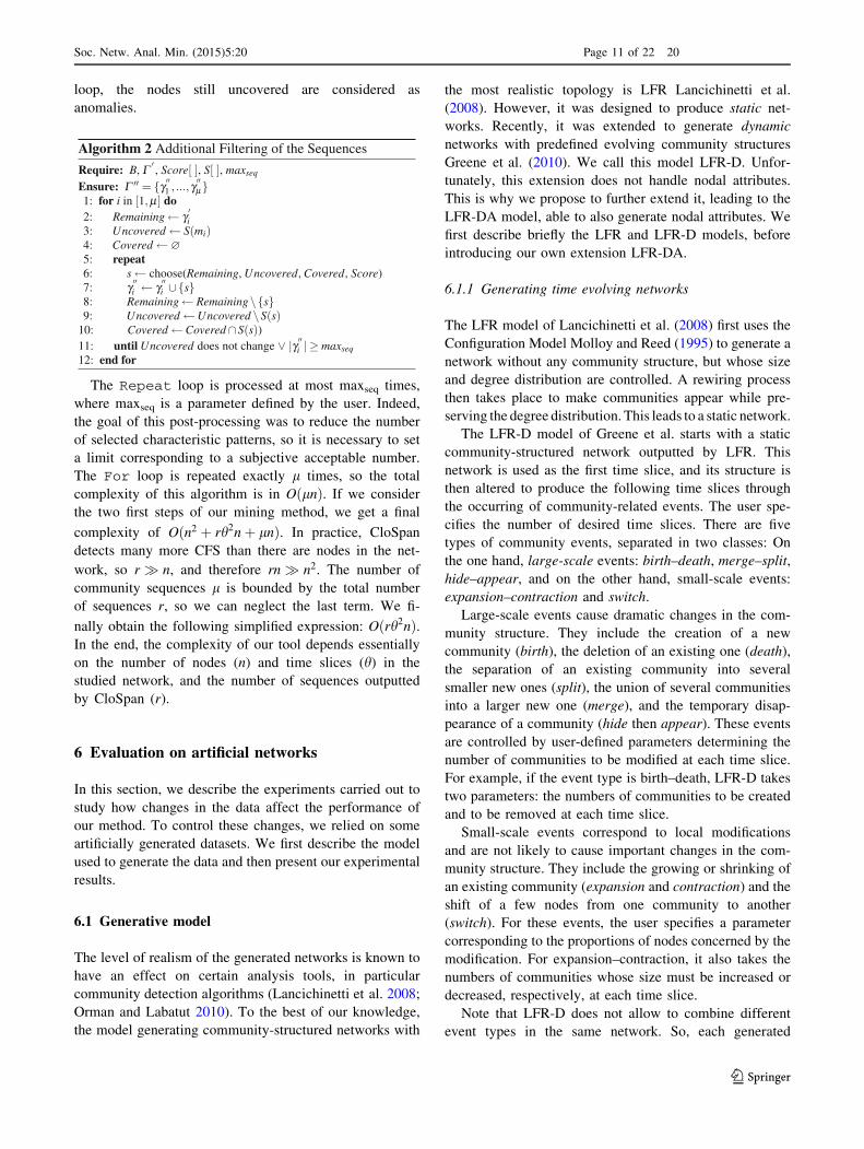
Figure 4 presents our results relatively to the effect of at-

tribute distribution. The plots are organized similarly to the

previous figures. CloSpan is the fastest (top-left plot) when

the attribute values are completely homogeneous (degen-

erate distribution) or completely heterogeneous (uniform

distribution). Because of the finite size of the attribute

domains, a uniform distribution leads to communities

containing groups of similar nodes of approximately the

same size. If the community is large enough, the trends of

these node groups will be represented as different super-

sequences of the same community sequence. If it is too

small, the minsup threshold will not be reached, and our tool

will not detect the sequences. However, since we use the

same attribute values for all communities in this ex-

periment, the total size of these small node groups over the

whole network is large enough to exceed the threshold.

When the attributes values are relatively homogeneous

(binomial distribution), the execution time is at its highest.

In this case, there are many nodes having the same value

for a given attribute and a few ones with different values. It

seems that these few numbers of nodes with different

values are causing the identification of many extra candi-

date sequences (top-right plot). For both binomial and

power-law distributions, we see a distinction between the

processing of small-scale events, which is faster than for

large-scale ones.

The results obtained in these three experiments validate

and complete the analysis as presented in Sect. 5 regarding

the computational complexity of our tool. They highlight

the fact that the computing time is also affected in practice

by the number of attributes (which directly influences r, the

number of CFS identified by CloSpan) and their distribu-

tion. Moreover, the process becomes harder when the

studied network undergoes large changes. This holds for

both the community structure and the attribute values.


123

7 Validation on real-world networks

We apply our method on two dynamic attributed networks

modeling real-world systems: the first is a co-authorship

network from the DBLP website, and the second is a

friendship network from the LastFM service.

We treated both of them in exactly the same way. First,

we removed the isolated nodes, which do not have any

interest in this context. Then, as explained in Sect. 5.1.1,

we used Incremental Louvain to detect communities. The

obtained modularity is larger than 0.6, for each time slice

and on both networks, which is a sign of well-separated

communities. The preprocessing of the descriptors corre-

sponds to what we described in Sect. 5.1.2, including the

clustering of the nine topological measures into three at-

tributes representing the position of the node at the local

(degree and transitivity), intermediate (community-related

measures), and global (centralities and eccentricity) levels.

The preparation of the attributes is system dependent and is

therefore described later.

We built the sequence database M from the resulting

descriptors and communities and applied the process as

described in Sect. 5.2. We interpreted all the identified

characteristic patterns, but it is obviously not possible to

present them all in this article. We therefore focus on the

most representative, interesting and/or relevant ones, in

terms of interpretation of the communities, in order to give

an example of how our method can be used and how to

comment its outputs.

7.1 DBLP dataset

7.1.1 Data and preprocessing

DBLP is a bibliographic Website focusing on Computer

Science works. We selected the dynamic co-authorship

network of Desmier et al. (2012), extracted from the DBLP

database. Each one of the 2145 nodes represents an author.

Two nodes are connected if the corresponding authors

published an article together. Each time slice corresponds

to a period of five years. There are ten time slices in total,

ranging from 1990 to 2012. The consecutive periods have a

three-year overlap for the sake of stability. For each author,

at each time slice, the database provides the number of

publications in 43 conferences and journals. We used this

information to define 43 nodal attributes corresponding

1 2 3 4 5

010

030

050

0Number of Attributes

Tim

e in

Sec

onds

1 2 3 4 5

Number of Attributes

Num

ber o

f Seq

uenc

es10

35

×10

410

5

1 2 3 4 5

9395

9799


Seq

uenc

es %

1 2 3 4 5

010

030

050

0


Tim

e in

Sec

onds

birth−death expansion−contraction hide−appear

merge−split switch

Fig. 2 Results of experiment 1:

execution time of CloSpan (top-

left), total number of sequences

found by CloSpan (top-right),

percentage of community-

related sequences (bottom-left),

and execution time for

emergence computation

(bottom-right), as functions of

the number of attributes jAj.Colors represent the different

types of community-related

events


123

directly to the individual conferences and journals and two

additional ones representing the total number of conference

and journal publications, respectively. We consequently

have a total of 45 nodal attributes.

The conference/journals we selected are related to the

subjects of database, data mining, knowledge discovery,

information retrieval, or artificial intelligence. To lighten

the computational load, we decided to bin their values. For

a journal/conference publication, we determined 5 cate-

gories, corresponding to the number of publications 1, 2, 3,

4, and greater or equal to 5. For both attributes representing

the total conference and journal publications, we defined

five categories as well, but they correspond to different

ranges: ½1; 5�; �5; 10�; �10; 20�; �20; 50� and �50;1½. These

thresholds were determined according to our knowledge of

the domain. For the mining step, we used minsup = 21

nodes, mingr = 1.00, and maxseq = 5. We obtained

1,106,108 closed frequent sequences with these parameter

values, 19,922 of which (’1%) were community related.

The total execution time for finding the CFS was ap-

proximately 400 s, whereas it was close to 6000 s for the

post-processing. Although the DBLP network has much

more descriptors than our artificially generated networks,

we see that these execution times are consistent with the

experimental results obtained on the LFR networks for the

same numbers of result patterns.

7.1.2 Interpretation

The communities of the DBLP network are very dy-

namic and change much through time. In the beginning

of the considered time period, the communities are in

general smaller. As time goes by, small communities

tend to merge into larger ones, appearing around

t = 7–9. Descriptor-wise communities are not described

by a single-characteristic pattern: several ones are re-

quired to get a sufficient coverage. Communities are not

homogeneous in terms of conference or journal, and

their members publish on several different scientific

platform.

As an example, we focus on a community appearing at

t = 6 (i.e., 2000–2004) and containing 120 nodes. Note

that, except at t = 6, these 120 nodes belong to several

different communities. We have found three characteristic

patterns for this community, which are listed, with their

interpretation, support, and growth rate, in Table 3. As

mentioned before, the topological descriptors have been

discretized by means of a cluster analysis. Instead of

0 20 40 60 80 100

010

030

050

0Evolution Percentage

Tim

e in

Sec

onds

0 20 40 60 80 100

Evolution Percentage

Num

ber o

f Seq

uenc

es

103

5×

106

107

0 20 40 60 80 100

2040

6080

100


Seq

uenc

es %

0 10 20 30 40 50

050

000

1500

00


Tim

e in

Sec

onds

birth−death expansion−contraction hide−appear

merge−split switch

Fig. 3 Results of experiment 2:









the evolution percentage q.

Colors represent the different


events


123

describing the patterns in terms of meaningless cluster

numbers, we name them using their most characteristic

feature (e.g., high embeddedness for the group of com-

munity-related measures). The evolution of the 120 nodes

at t = 2, 4, 6, 8, and 10 is represented in Fig. 5. Their

colors represent which ones of the community character-

istic patterns they support, and their sizes are proportional

to the number of supported patterns. For readability mat-

ters, at each time slice, we show only the nodes belonging

to the largest community.

As shown in figure, most of the nodes do not belong to

the same community in the first time slices. They gather

together at t = 6 time and split again later. This commu-

nity is not homogeneous around one conference or journal,

since we identified three characteristic patterns involving

different scientific platforms (SDM, ICDM, and TKDE).

However, all of them are related to data mining, so the

community is thematically homogeneous. The topological

information present in all three patterns describes nodes

strongly belonging to their community and critical for in-

formation flow (high betweenness). Pattern #1 shows that,

after publishing in SDM once, the nodes get connections

with many other communities (high participation coeffi-

cient). Considering the growth rate of the patterns #1, 2 and

3, we conclude that these patterns are not highly emergent

for this community. Investigating its reason, we see that in

the network, there are other nodes with similar trends.

Nevertheless, these other nodes are not neighboring the

community of interest.

Table 3 also shows the characteristic pattern for another

community, appearing at t = 8 and containing 113 nodes.

This pattern tells us the community contains a group of

nodes which publish at ILP once and then get high be-

tweenness and embeddedness, whereas their closeness gets

low. As it is seen in table, the growth rate of the pattern is

very high, which means that the nodes supporting it con-

stitute a distinctive trend in the community.

7.2 LastFM dataset

7.2.1 Data and preprocessing

LastFM is a music Website that allows its members to

register and listen to music online. It is also a social net-

work platform because the members can declare friendship

relationships. In LastFM, members can join predefined

groups related to their music tastes and declare their par-

ticipation to music-related events such as concerts. We

Distribution TypeTi

me

in S

econ

ds0

100

300

500

Distribution Type

Num

ber o

f Seq

uenc

es

103

5×

105

106

degenerate binomial power law uniformdegenerate binomial power law uniform

degenerate binomial power law uniform degenerate binomial power law uniform

birth−death expansion−contraction hide−appearmerge−split switch

Distribution Type

Seq

uenc

es %

020

4060

8010

0

Distribution TypeTi

me

in S

econ

ds0

2000

4000

6000

8000

Fig. 4 Results of Experiment 3:









the attributes distribution h.

Colors represent the different


events


123

extracted a network by focusing on the members of the

Jazz group, which is supposed to include users appreciating

this type of music.

We took advantage of the LastFM API and of the Jazz

group statistics provided by LastFM to retrieve its mem-

bers and identify the highest rated artists and event types

for this group. It is interesting to notice that, although all

the members we are interested in are from the Jazz group,

the selection of the most popular artists includes acts from

music types which are very different from Jazz, such as the

Beatles or Pink Floyd. We nevertheless kept these artists

because their playing rate is very high for the group. Event

types also span a wide range of music types, from Jazz to

Folk. We tracked the activity of the Jazz group members

for the year 2013. We created a time evolving network

containing 3478 nodes (each one representing a users from

the Jazz group) and including 12 time slices (each one

representing a 1-month period).

We defined 37 nodal attributes based on the users’ music

tastes: 21 of them represent the most popular artists in the

Jazz group, and the 16 others correspond to the types of

events the members can join. For each time slice, the at-

tribute values correspond to the total numbers of times a

given user listened to a given artist, and the number of

times he joined an event of a given type, respectively. We

put a link between two nodes if two conditions were

simultaneously true: (1) both considered users listened to at

least one common artist for a specific period of time, and

(2) they declared a friendship relation on the LastFM

platform.

Once the network was created, we processed the re-

quired topological measures and clustered them as we did

for the DBLP network. The attribute values were binned.

For artist attributes, we determined five intervals regarding

the numbers of listenings: ½1; 5�; �5; 30�; �30; 90�; �90; 200�and �200;1½. Regarding the event types, we defined four

intervals: ½1; 4�; �4; 7�; �7; 11� and �11;1½. These thresholds

were determined according to our knowledge of the do-

main. For mining, we used minsup = 15 nodes,

mingr = 1.00, and maxseq = 5. With these parameter val-

ues, we found 632; 037 closed frequent patterns, 44,631 of

which (’7%) were community related. The total execution

time for finding the CFS was close to 200 s, whereas ut was

approximately 7000 s for post-processing. Like for DBLP,

we see that the LastFM execution times are consistent with

the results obtained on LFR networks.

7.2.2 Interpretation

The evolution of the LastFM communities is generally

smoother than for DBLP. We observe relatively large

communities at t = 1 and 2, and communities tend to

Fig. 5 Evolution of a community of 120 nodes appearing at t ¼ 6.

Nodes not following any characteristic patterns are represented in

black. Red, yellow, and blue nodes follow one of the three

characteristic patterns. Orange, purple, and green nodes follow two

patterns, and the cyan node follows all three characteristic patterns.

The node size represents the number of supported characteristic

patterns. Pattern-related details are given in Table 3


123

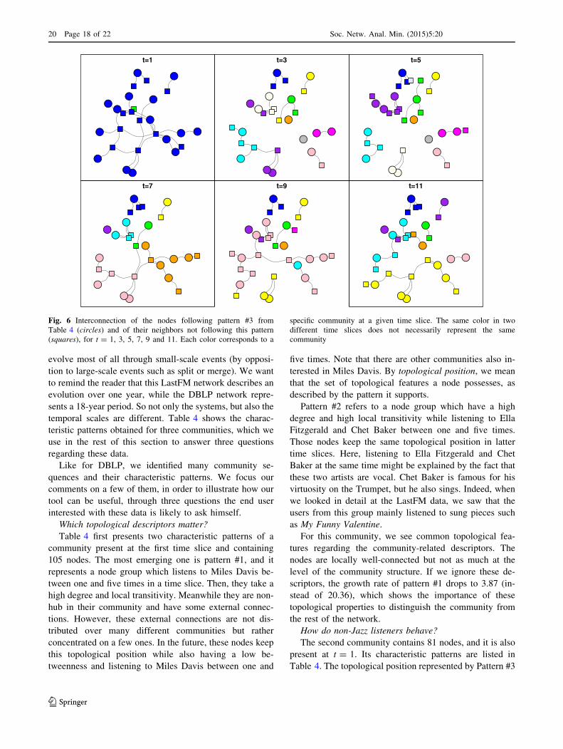
evolve most of all through small-scale events (by opposi-

tion to large-scale events such as split or merge). We want

to remind the reader that this LastFM network describes an

evolution over one year, while the DBLP network repre-

sents a 18-year period. So not only the systems, but also the

temporal scales are different. Table 4 shows the charac-

teristic patterns obtained for three communities, which we

use in the rest of this section to answer three questions

regarding these data.

Like for DBLP, we identified many community se-

quences and their characteristic patterns. We focus our

comments on a few of them, in order to illustrate how our

tool can be useful, through three questions the end user

interested with these data is likely to ask himself.

Which topological descriptors matter?

Table 4 first presents two characteristic patterns of a

community present at the first time slice and containing

105 nodes. The most emerging one is pattern #1, and it

represents a node group which listens to Miles Davis be-

tween one and five times in a time slice. Then, they take a

high degree and local transitivity. Meanwhile they are non-

hub in their community and have some external connec-

tions. However, these external connections are not dis-

tributed over many different communities but rather

concentrated on a few ones. In the future, these nodes keep

this topological position while also having a low be-

tweenness and listening to Miles Davis between one and

five times. Note that there are other communities also in-

terested in Miles Davis. By topological position, we mean

that the set of topological features a node possesses, as

described by the pattern it supports.

Pattern #2 refers to a node group which have a high

degree and high local transitivity while listening to Ella

Fitzgerald and Chet Baker between one and five times.

Those nodes keep the same topological position in latter

time slices. Here, listening to Ella Fitzgerald and Chet

Baker at the same time might be explained by the fact that

these two artists are vocal. Chet Baker is famous for his

virtuosity on the Trumpet, but he also sings. Indeed, when

we looked in detail at the LastFM data, we saw that the

users from this group mainly listened to sung pieces such

as My Funny Valentine.

For this community, we see common topological fea-

tures regarding the community-related descriptors. The

nodes are locally well-connected but not as much at the

level of the community structure. If we ignore these de-

scriptors, the growth rate of pattern #1 drops to 3.87 (in-

stead of 20.36), which shows the importance of these

topological properties to distinguish the community from

the rest of the network.

How do non-Jazz listeners behave?

The second community contains 81 nodes, and it is also

present at t = 1. Its characteristic patterns are listed in

Table 4. The topological position represented by Pattern #3

Fig. 6 Interconnection of the nodes following pattern #3 from

Table 4 (circles) and of their neighbors not following this pattern

(squares), for t = 1, 3, 5, 7, 9 and 11. Each color corresponds to a

specific community at a given time slice. The same color in two

different time slices does not necessarily represent the same

community


123

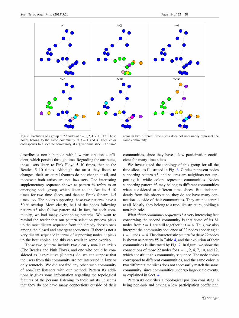
describes a non-hub node with low participation coeffi-

cient, which persists through time. Regarding the attributes,

these users listen to Pink Floyd 5–10 times, then to the

Beatles 5–10 times. Although the artist they listen to

changes, their structural features do not change at all, and

moreover both artists are not Jazz acts. One interesting

supplementary sequence shown as pattern #4 refers to an

emerging node group, which listen to the Beatles 5–10

times for two time slices, and then to Frank Sinatra 1–5

times too. The nodes supporting these two patterns have a

50 % overlap. More clearly, half of the nodes following

pattern #3 also follow pattern #4. In fact, for each com-

munity, we had many overlapping patterns. We want to

remind the reader that our pattern selection process picks

up the most distant sequence from the already chosen ones

among the closed and emergent sequences. If there is not a

very distant sequence in terms of supporting nodes, it picks

up the best choice, and this can result in some overlap.

Those two patterns include two clearly non-Jazz artists

(The Beatles and Pink Floys), and one who could be con-

sidered as Jazz-relative (Sinatra). So, we can suppose that

the users from this community are not interested in Jazz or

only remotely. We did not find any other such community

of non-Jazz listeners with our method. Pattern #3 addi-

tionally gives some information regarding the topological

features of the persons listening to these artists. It seems

that they do not have many connections outside of their

communities, since they have a low participation coeffi-

cient for many time slices.

We investigated the topology of this group for all the

time slices, as illustrated in Fig. 6. Circles represent nodes

supporting pattern #3, and squares are neighbors not sup-

porting it, while colors represent communities. Nodes

supporting pattern #3 may belong to different communities

when considered at different time slices. But, indepen-

dently from this observation, they do not have many con-

nections outside of their communities. They are not central

at all. Mostly, they belong to a tree-like structure, holding a

non-hub role.

What about community sequences?Avery interesting fact

concerning the second community is that some of its 81

nodes from t = 1 are still together at t = 4. Thus, we also

interpret the community sequence of 22 nodes appearing at

t = 1 and t = 4. The characteristic pattern for these 22 nodes

is shown as pattern #5 in Table 4, and the evolution of their

communities is illustrated by Fig. 7. In figure, we show the

connections of those 22 nodes for t = 1, 2, 4, 7, 10, and 12,

which constitute this community sequence. The node colors

correspond to different communities, and the same color in

two different time slices does not necessarily match the same

community, since communities undergo large-scale events,

as explained in Sect. 4.

Pattern #5 describes a topological position consisting in

being non-hub and having a low participation coefficient.

Fig. 7 Evolution of a group of 22 nodes at t ¼ 1; 2; 4; 7; 10; 12. Thosenodes belong to the same community at t = 1 and 4. Each color

corresponds to a specific community at a given time slice. The same

color in two different time slices does not necessarily represent the

same community


123

Attribute-wise, these users listen to Pink Floyd 5–10 times.

This trend is very similar to that of the larger community

we discussed just before (patterns #3 and 4). This smaller

sequence shows us that some nodes with similar interest

keep their connections for several time slices, even if the

rest of their community changes. The support of pattern #5

shows that this smaller community is more homogeneous

than the larger community. The same observation can be

done for many other communities in our results as well.

This could be interpreted as the presence of a certain

hierarchical structure in the network, defined in terms of

both topology and attributes (i.e., nested interests). How-

ever, a more thorough study shows that this type of hier-

archy is not stable through time. For this reason, it is more

accurate to consider that communities have one or several

cores, corresponding to nodes supporting long sequences,

i.e., evolving together for a long time. These cores can

overlap and switch communities. They are joined punctu-

ally by other cores or peripheral nodes to form short-ter-

med communities. The way those node groups move in the

community structure could be studied to understand how

trends propagate through a network.

7.3 Discussion

Let us conclude the analysis of the real-world networks

with a comparison of the obtained results. Regarding the

time performance, we can say that although both networks

have smaller sizes and much more node descriptors than

the generated artificial networks considered in Sect. 7, the

percentage of community-related sequences we identified

is larger by less than 7 %. This makes the execution time of

the growth rate computation lower than for most of these

artificial networks. One reason for this observation can be

the minimum support threshold we used, which puts a limit

to the community sizes. As a result, there are fewer com-

munity-related sequences. About the execution time of the

CFS mining, we know the numbers of node descriptors

affect it. So, we expected that it would run slower for our

real-world networks, which contain many descriptors.

However, our results show that there is no significant dif-

ference between the performances obtained on artificial

and real-world networks. One reason for this could be the

heterogeneity of the descriptor values over the nodes: it

leads to the generation of less candidate sequences, and

CloSpan consequently works faster than expected.

The community structure of both networks changes very

much at each time slice, especially for DBLP. The com-

munities in this network are getting larger with time,

whereas for LastFM, their sizes remain relatively constant.

For a large part of the communities, the most supported

sequences involve mainly topological descriptors. For

DBLP, inside a given community, almost all the nodes

(*90 %) have the same topological situation. For most of

the communities, this situation is being non-hub and having

a low participation coefficient. But certain communities are

also characterized by non-central, low degree nodes. For

LastFM, we also find purely topological sequences, in

particular being non-hub and having a zero or low par-

ticipation coefficient. But a number of sequences also re-

flect an interest towards specific Jazz artists. The

proportion of nodes following the most supported se-

quences is not as high as for DBLP (*70 %).

It is worth noting the combination of topological and

attribute-based descriptors help interpreting the patterns:

changes in the topological aspect can help explaining

changes in the attributes and vice-versa. For example, in

Table 3, pattern #1 displays a changes in the topological

features: the nodes have at first a high embeddedness,

which means that most of their neighbors are in the same

community. Then, they publish in SDM and then have a

high participation coefficient, meaning that they get con-

nected to (many) other communities: this can correspond to

the beginning of new collaborations started after having

published in a prestigious conference. On the contrary,

node groups which are more embedded in their commu-

nities keep publishing in the same conferences.

For both networks, we cannot claim that the communi-

ties are constituted of nodes gathering around a single in-

terest. The characteristic patterns show us several distinct

trends exist simultaneously in the same community. So, the

communities are not homogeneous in terms of patterns.

However, note that the term homogeneous applies here to

the descriptors constituting the patterns: different descrip-

tors, especially nodal attributes, can actually have very

close meanings. For instance, we showed that a community

of DBLP was characterized by several distinct patterns all

related to journals and conferences from the Data Mining

filed, i.e., thematically very similar.

The existence of several trends for the same communi-

ties means that we have distinct subgroups of nodes sup-

porting them. These subgroups are mobile, in the sense,

they switch from one community to the other. This is re-

lated to our previous remark regarding the fact that the

community structures of these networks are significantly

changing from one time slice to the other. This can be a

feature of the studied system, but it can also be an artifact

of the community detection method, so this point should be

considered carefully when applying our method.

8 Conclusion and perspectives

In this work, we tackled the task of interpreting commu-

nities detected in dynamic attributed complex networks.

We first formalized it as a data mining problem, then


123

proposed a method to solve it. It is based on a sequence-

based representation of the information, allowing to store

simultaneously the topological information, the node at-

tributes, the community structure, and the temporal di-

mension. Our method takes advantage of this

representation to search for frequent closed emerging se-

quential patterns, in order to characterize each community.

This step involves the use of the data mining tool CloSpan

Yan et al. (2003). To our knowledge, this is the first time

that the task of interpreting communities is formulated as a

problem, moreover independently from the community

detection task. Our goal was to overcome the limitations of

the few existing studies (Labatut and Balasque 2012;

Tumminello et al. 2011; Lancichinetti et al. 2010) by

proposing a systematic approach, taking into account the

topological structure, the nodal attributes, and the network

dynamics. Our sequential representation has not been used

for graphs before. The process we proposed to extract the

most relevant patterns based on closed and emergent se-

quences relatively to the communities is original.

Using artificially generated networks, we studied how

our method is affected by certain properties of the treated

data. To this aim, we proposed an extension of an existing

generative model Greene et al. (2010), allowing to produce

dynamic attributed networks possessing a community

structure. These empirical results confirm the analytic ex-

pression that we provided for the algorithmic complexity of

our method and the effect of the network size (both in

terms of nodes and time slices) and of the number of de-

tected closed frequent patterns (itself related to the number

of considered descriptors). We also used two real-world

networks to validate our method. The first is a DBLP

network showing the evolution of co-authorship connec-

tions over 18 years. We identified the presence of several

trends in most communities, corresponding to subgroups

focusing on different journals and conferences. These sci-

entific platforms are connected to the same field, though

(e.g., Data Mining, Artificial Intelligence, etc.), which re-

veals a certain thematic homogeneity in a community. The

second network is extracted from LastFM and represents

the evolution of Jazz listeners, their friendship relations,

and listening habits for the year 2013. For this network, we

also characterized thematically certain communities, de-

pending on their favorite artists. We also identified a group

of users which actually do not listen to Jazz.

In the future, we plan to apply our method to the ana-

lysis of other types of networks, in order to explore further

its characterization capabilities. A related point consists in

identifying which descriptors are the most relevant to de-

scribe a given system. For those considered here, the

community-based topological measures were very dis-

criminant, but this is not necessarily true for other systems.

The preprocessing of the descriptors is also a critical point

that we want to explore. The main limitation of our method

is its computational costs, which is due to the pattern

mining perspective we adopted. Identifying the most im-

portant descriptors or performing a more appropriate pre-

processing would allow to reduce the search space and

therefore to eliminate some redundant CFS, to ease the

identification of emerging patterns, and to make the post-

processing faster. We also plan to improve our method

itself, noticeably using hash maps to process emergence.

References

Aynaud T, Guillaume J-L (2010) Static community detection

algorithms for evolving networks. In: Modeling and optimization

in mobile, ad hoc and wireless networks (WiOpt), 2010

proceedings of the 8th international symposium on, pp 513–519

Blondel VD, Guillaume J-L, Lambiotte R, Lefebvre E (2008) Fast

unfolding of communities in large networks. J Stat Mech

10:P10008

Blondel VD (2011) The Louvain method for community detection in

large networks. http://perso.uclouvain.be/vincent.blondel/

research/louvain.html

Bonacich P (1987) Power and centrality: a family of measures. Am J

Sociol 92(5):1170–1182

Chen J, Tang Y, Li J, Mao C, Xiao J (2014) Community-based

scholar recommendation modeling in academic social network

sites. In: Huang Z, Liu C, He J, Huang G (eds) Web information

systems engineering WISE 2013 workshops. Lecture notes in

computer science. Springer, Berlin, pp 325–334

Desmier E, Plantevit M, Robardet C, Boulicaut J-F (2012) Cohesive

co-evolution patterns in dynamic attributed graphs. In: Ganascia

J-G, Lenca P, Petit J-M (eds) Discovery science. Lecture notes in

computer science. Springer, Berlin, pp 110–124

Dong G, Li J (1999) Efficient mining of emerging patterns:

discovering trends and differences. In: Proceedings of the fifth

ACM SIGKDD international conference on knowledge discov-

ery and data mining, KDD ’99, ACM, New York, pp 43–52

Dugue N, Labatut V, Perez A (2014) Identification de roles commu-

nautaires dans des reseaux orientes applique twitter. In: 14eme

Conference Extraction et Gestion des Connaissances (EGC)

Fortunato S (2010) Community detection in graphs. Phys Rep

486(3–5):75–174

Fortunato S, Lancichinetti A (2009) Community detection algorithms:

a comparative analysis: invited presentation, extended abstract.

In: Proceedings of the fourth international ICST conference on

performance evaluation methodologies and tools, VALUE-

TOOLS ’09, ICST (Institute for Computer Sciences, Social-

Informatics and Telecommunications Engineering). ICST, Brus-

sels, pp 27:1–27:2

Freeman L (1979) Centrality in social networks I: conceptual

clarification. Soc Netw 1(3):215–239

Gallo A, De Bie T, Cristianini N (2007) Mini: mining informative

non-redundant itemsets. Knowledge Discovery in Databases:

PKDD 2007. Lecture notes in computer science. Springer,

Berlin, pp 438–445

Girvan M, Newman MEJ (2002) Community structure in social and

biological networks. Proc Natl Acad Sci USA 99(12):7821–7826

Greene D, Doyle D, Cunningham P (2010) Tracking the evolution of

communities in dynamic social networks. In: Advances in social

networks analysis and mining (ASONAM), 2010 international

conference on, pp 176–183


123

http://perso.uclouvain.be/vincent.blondel/research/louvain.html

http://perso.uclouvain.be/vincent.blondel/research/louvain.html

Guimera R, Amaral LAN (2005) Cartography of complex networks:

modules and universal roles. J Stat Mech 2005(02):P02001

Gusfield JR (1975) Community: a critical response. Harper & Row,

New York

Harary F (1969) Graph theory. Addison-Wesley Publishing Company,

Boston

Labatut V, Balasque J-M (2012) Detection and interpretation of

communities in complex networks: practical methods and

application. In: Abraham A, Hassanien A-E (eds) Computational

social networks. Springer, London, pp 81–113

Labatut V, Balasque J-M (2013) Informative value of individual and

relational data compared through business-oriented community

detection. In: Ozyer T, Rokne J, Wagner G, Reuser AH (eds)

The influence of technology on social network analysis and

mining. Lecture notes in social networks. Springer, Vienna,

pp 303–330

Lancichinetti A, Fortunato S, Radicchi F (2008) Benchmark graphs

for testing community detection algorithms. Phys Rev E 78(4 Pt

2):046110

Lancichinetti A, Kivela M, Saramaki J, Fortunato S (2010) Charac-

terizing the community structure of complex networks. PLoS

One 5(8):e11976

Leskovec J, Adamic LA, Huberman BA (2007) The dynamics of viral

marketing. ACM Trans Web 1:5

Leskovec J, Lang KJ, Dasgupta A, Mahoney MW (2008) Statistical

properties of community structure in large social and informa-

tion networks. In: 17th international conference on World Wide

Web, series statistical properties of community structure in large

social and information networks, pp 695–704

Li Z, Lu S, Myagmar S, Zhou Y (2006) Cp-miner: finding copy-paste

and related bugs in large-scale software code. IEEE Trans Softw

Eng 32(3):176–192

McMillan DW, Chavis DM (1986) Sense of community: a definition

and theory. J Commun Psychol 14:6–23

Molloy M, Reed B (1995) A critical point for random graphs with a

given degree sequence. Random Struct Algorithms 6(2/

3):161–179

Newman MEJ (2003) The structure and function of complex

networks. SIAM Rev 45:167–256

Orman GK (2014) Contribution to the interpretation of evolving

communities in complex networks: application to the study of

social interactions. Ph.D. thesis, INSA, Lyon

Orman GK, Labatut V (2010) The effect of network realism on

community detection algorithms. In: ASONAM, series the effect

of network realism on community detection algorithms, Odense,

pp 301–305

Parau P, Stef A, Lemnaru C, Dinsoreanu M, Potolea R (2013) Using

community detection for sentiment analysis. In: Intelligent

computer communication and processing (ICCP), 2013 IEEE

international conference on, pp 51–54

Pei J, Han J, Mortazavi-Asl B, Pinto H, Chen Q, Dayal U, Hsu M

(2001) Prefixspan: mining sequential patterns by prefix-projected

growth. In: Proceedings of the 17th international conference on

data engineering, IEEE Computer Society, Washington, DC,

pp 215–224

Rosvall M, Bergstrom CT (2008) Maps of random walks on complex

networks reveal community structure. Proc Natl Acad Sci USA

105(4):1118

Rousseeuw P (1987) Silhouettes: a graphical aid to the interpretation

and validation of cluster analysis. J Comput Appl Math 20:53–65

Sabidussi G (1966) The centrality index of a graph. Psychometrika

31(4):581–603

Stattner E, Collard M (2012) Social-based conceptual links: concep-

tual analysis applied to social networks. In: Advances in social

networks analysis and mining (ASONAM), 2012 IEEE/ACM

international conference on, pp 25–29

Tumminello M, Micciche S, Lillo F, Varho J, Piilo J, Mantegna RN

(2011) Community characterization of heterogeneous complex

systems. J Stat Mech 2011(01):P01019

Watts DJ, Strogatz SH (1998) Collective dynamics of ’small-world’

networks. Nature 393(6684):440–442

Yan X, Han J, Afshar R (2003) Clospan: mining closed sequential

patterns in large datasets. In: Proceedings 2003 international

SIAM conference on data mining (SDM ’03), pp 166–177

Yang J, McAuley J, Leskovec J (2013) Community detection in

networks with node attributes. In: Data Mining (ICDM), 2013

IEEE 13th international conference on, pp 1151–1156

Zaki MJ, Hsiao C-J (2002) Charm: an efficient algorithm for closed

itemset mining. In: Grossman RL, Han J, Kumar V, Mannila H,

Motwani R (eds) SDM. SIAM, Arlington

Zhou Y, Cheng H, Yu J (2009) Graph clustering based on structural/

attribute similarities. Proc VLDB Endow 2:718–729


123

interpreting communities based on the evolution of a

Documents