“Interpreting factor models”, by Kozak, Nagel, and Santosh

Discussant: Annette Vissing-Jorgensen, UC Berkeley

Empirical results:

The returns studied have rapidly decaying eigenvalues (a few orthogonal vectors

account for a large part of the variation in returns).

Therefore, if you assume expected returns are driven by covariances, they have to

be driven by covariances with a small number of principal components of returns.

If not, implausibly large Sharpe ratios would be obtainable.

Out-of-sample squared Sharpe ratios max out around 1 (in one case higher).

The authors do not consider this implausibly large, consistent with expected

returns being driven by covariances.

“Small” appears to be 7 in the data (based on how many principal components you

need to load on in order to maximize your out-of-sample Sharpe ratio).

Theoretical results:

Expected returns will be driven by covariances even if some investors’ portfolios

deviate from the rational one as long as:

(1) There are arbitrageurs in the model, and

(2) Irrational investors have a “budget constraint” for irrationality.

Therefore, the characteristic vs. covariances literature for testing whether

investors and asset prices are rational is not useful.

Related, the investment based asset pricing literature is also not useful for testing

whether investors are rational is also not useful. It builds on firm rationality, but

doesn’t have anything to say about whether investors and asset prices are rational.

Overall, not a very uplifting paper!

Comment 1. I’m not quite sure what to make of the empirical part

The test for whether expected returns are plausibly driven by covariances is whether

the out-of-sample Sharpe ratio is “too big”, but there is little discussion of what is “too

big”.

In a CCAPM, the maximum squared Sharpe ratio is [(E(R)-Rf)/σ(R)]2 =[σ(m)/E(m)]2

(Cochrane, Chapter 1).

We have decades of research arguing that it’s hard to rationalize the Sharpe ratio

on the market (around 0.4, implying a squared SR of 0.16).

- For CRRA utility, [σ(m)/E(m)]2≈γ2 V(ΔlnC)

- V(ΔlnC) is around 0.0262 (1929-2014 data)

- To rationalize [σ(m)/E(m)]2=0.16, you need γ=15.

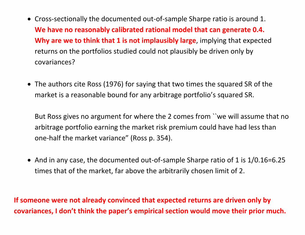
Cross-sectionally the documented out-of-sample Sharpe ratio is around 1.

We have no reasonably calibrated rational model that can generate 0.4.

Why are we to think that 1 is not implausibly large, implying that expected

returns on the portfolios studied could not plausibly be driven only by

covariances?

The authors cite Ross (1976) for saying that two times the squared SR of the

market is a reasonable bound for any arbitrage portfolio’s squared SR.

But Ross gives no argument for where the 2 comes from ``we will assume that no

arbitrage portfolio earning the market risk premium could have had less than

one-half the market variance” (Ross p. 354).

And in any case, the documented out-of-sample Sharpe ratio of 1 is 1/0.16=6.25

times that of the market, far above the arbitrarily chosen limit of 2.

If someone were not already convinced that expected returns are driven only by

covariances, I don’t think the paper’s empirical section would move their prior much.

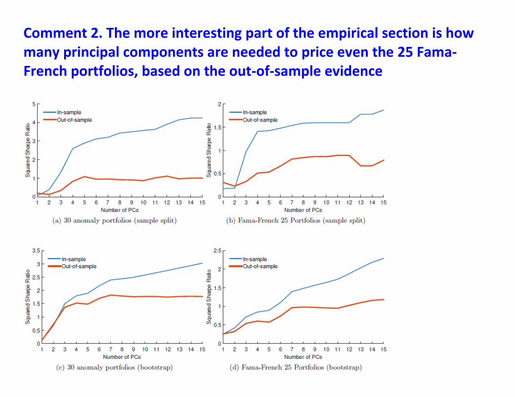
Comment 2. The more interesting part of the empirical section is how many principal components are needed to price even the 25 Fama-French portfolios, based on the out-of-sample evidence

There is a lot more (undiversifiable) structure to the 25 portfolios than I thought, even in

an economic sense (i.e., not just in that you statistically can reject the 3-factor model).

You can double your out-of-sample squared Sharpe ratio by investing in seven PCs

rather than three.

I’d like to know more about what the 4th to 7th PC loads on.

Aside from this issue mattering a lot for investors, it may be informative for our models.

Most models have a couple of shocks, but the results may indicate that we need

many more.

It would be helpful to combine the two sets of test assets to fully assess the number

of shocks needed (i.e. work with 30, or perhaps 30 minus size and value, plus 25 FF

portfolios).

Comment 3. I don’t agree that the investment-based asset pricing

literature shouldn’t move your prior about investor rationality

These models show that even if asset pricing is completely rational, you will

observe higher average (and expected) returns for value firms and small firms

and firm with low investments or high profitability due to firms reacting

rationally to cross-firm differences in cash flow covariances with the SDF and thus

in the cost of capital.

These models did move my prior towards rationality: Without them, you’d be

more likely to think value and small firm effects would have to be behavioral.

I don’t think they were ever intended to rule out behavioral asset pricing.

They are intended to make it harder to rule out rational asset pricing by

providing models where rational firms generate value and size effects, even if

investors are also rational. That is an important contribution.

So the investments-based literature says:

Don’t rule out rational asset pricing just because you see size or value effects.

Similarly, the sentiment theory model of the current paper says:

Don’t rule out behavioral asset pricing even if you see moderate Sharpe ratios and

expected returns lining up with covariances. The cross-section of expected returns

could still be driven purely by behavioral factors.

Both are useful contributions.

I think the authors of investment-based models understand that these models make no

assumption about investor rationality.

For example, Fama and French (JFE, 2015) is an empirical paper in the

investment-based area.

After stating the definition of a present value of a dividend stream

they state:

In addition to showing that observed facts could be consistent with rationality by

investors and firms, the investment-based models are also useful because they exploit

firm rationality to learn which firms have bad covariance properties:

If:

(1) There is cross-firm differences in the covariance of firm cash flows with the SDF

and thus in the cost of capital

(2) Firms observe these differences in the cost of capital and react rationally to

them,

then, you can learn something about which firms have high covariances of firm cash

flows and the SDF by sorting firms based on size, B/M, investment and profitability.

Now you (the researcher) have been told the identity of firms with high

covariances of cash flows with the SDF.

Now you can start studying what exactly these firms are doing different to

generate differences in covariances.

That’s a meaningful step forward to understand where risk comes from and one

that may help shed light on the rational vs. behavioral investor debate.

- For example, suppose firms with high expected returns based on size, B/M,

investment and profitability sorts turned out to be mainly firms with

products very visible to consumers.

You’d probably conclude that sentiment shocks for these stocks contributed

a lot to arbitrageurs requiring a high expected returns to hold them.

- Or, suppose firms with high expected returns based on size, B/M, investment

and profitability sorts turned out to be mainly firms with products that are

technically very complex to understand (gene therapy, say).

You may conclude that ``limited participation’’ in such stocks due to

informational complexity may rationally help drive their risk premia.

Furthermore, by sorting firms based on more than just two variables (size and B/M), we

get expanded sets of test assets with large spreads in expected returns.

This is useful for overcoming the problem of many models potentially being able to

provide a decent fit on the 25 FF portfolios

(See Lewellen, Nagel and Shanken (2010 and Daniel and Titman (2012) for a

discussion of the need to sort on more than two dimensions.)

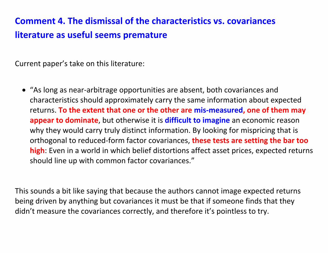
Comment 4. The dismissal of the characteristics vs. covariances

literature as useful seems premature

Current paper’s take on this literature:

“As long as near-arbitrage opportunities are absent, both covariances and characteristics should approximately carry the same information about expected returns. To the extent that one or the other are mis-measured, one of them may appear to dominate, but otherwise it is difficult to imagine an economic reason why they would carry truly distinct information. By looking for mispricing that is orthogonal to reduced-form factor covariances, these tests are setting the bar too high: Even in a world in which belief distortions affect asset prices, expected returns should line up with common factor covariances.”

This sounds a bit like saying that because the authors cannot image expected returns being driven by anything but covariances it must be that if someone finds that they didn’t measure the covariances correctly, and therefore it’s pointless to try.

This is a confusing message:

1) It doesn’t seem to appreciate the Daniel and Titman (1997) methodology The charateristics vs. covariances literature is not just regressing expected returns on characterics and covariances to see what matters most, it is double sorting.

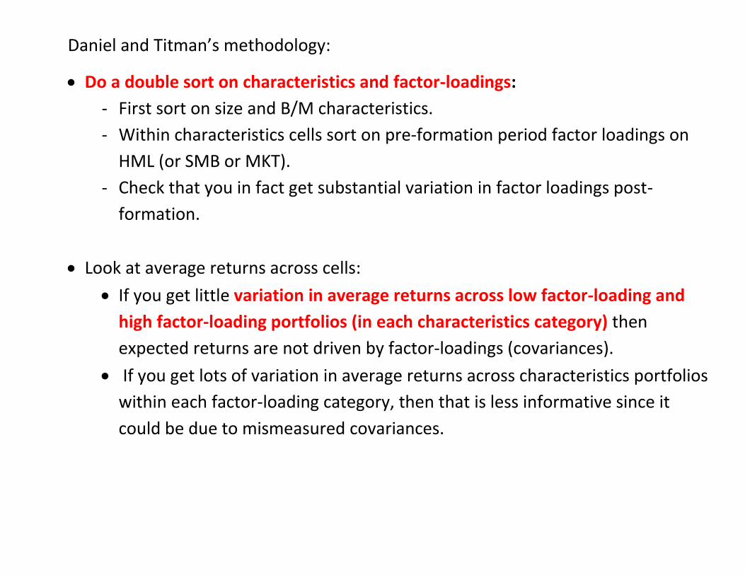
Daniel and Titman’s methodology:

Do a double sort on characteristics and factor-loadings:

- First sort on size and B/M characteristics.

- Within characteristics cells sort on pre-formation period factor loadings on

HML (or SMB or MKT).

- Check that you in fact get substantial variation in factor loadings post-

formation.

Look at average returns across cells:

If you get little variation in average returns across low factor-loading and

high factor-loading portfolios (in each characteristics category) then

expected returns are not driven by factor-loadings (covariances).

If you get lots of variation in average returns across characteristics portfolios

within each factor-loading category, then that is less informative since it

could be due to mismeasured covariances.

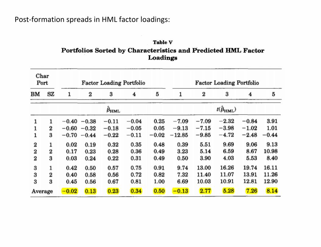
Post-formation spreads in HML factor loadings:

Post-formation average returns:

Time-series tests for characteristics-balanced portfolios (long factor loading

portfolio 1 and 2 and short factor-loading portfolio 4 and 5):

From this, Daniel and Titman conclude that: “…, our evidence suggests that it is characteristics rather than factor loadings that determine expected returns. We show that factor loadings do not explain the high returns associated with small and high book-to-market stocks beyond the extent to which they act as proxies for these characteristics.”

If that conclusion is wrong then the problem is not that covariances are poorly

measured but that the lack of risk premium is specific to a particular sample

(1973-1993 in Daniel and Titman).

- Davis, Fama and French (2000) found that Daniel and Titman’s results were

not present using data from 1929-1972 and 1994-1997.

- Daniel, Titman and Wei (2001) replied by showing additional out-of-sample

evidence, finding B/M characteristics to be more important than HML factor

loadings in Japanese stock returns.

2) It does not appreciate a potential role for limits to arbitrage It is not obvious that characteristics will never matter and by studying when they do/do not matter we are learning something about when behavioral biases matter most. Example: Stambaugh, Yu and Yuan (2012) study a similar set of anomalies

- They show that the majority of anomaly profits are made in times of high sentiment

- This is due to the stocks in the short leg losing value in times of high sentiment (thus making money when you short them)

- Suggests that arbitrageurs do not succeed in preventing over-pricing during high sentiment periods, likely because they are not shorting enough

- So perhaps characteristics may sometimes matter, even if only covariances matter when constraints are not binding.

3) More generally, but less to the point of the rational/behavioral debate, there are lots of priced characteristics in asset markets (things that drive expected returns without doing so via covariances):

- Banks paying “too much” for Greek government bond pre-crisis because of low risk-weights

- Rich investors paying “too much” for muni-bonds because of their low tax rates

- Hedge funds paying “too much” for Treasuries because of their liquidity. - Grandmothers paying “too much” for bank deposits because the

informational cost to them of understanding any risky investment is large.

The authors’ point that both rational and behavioral investors can drive expected returns via covariances is well taken, but we should still focus a lot on characteristics in asset pricing.

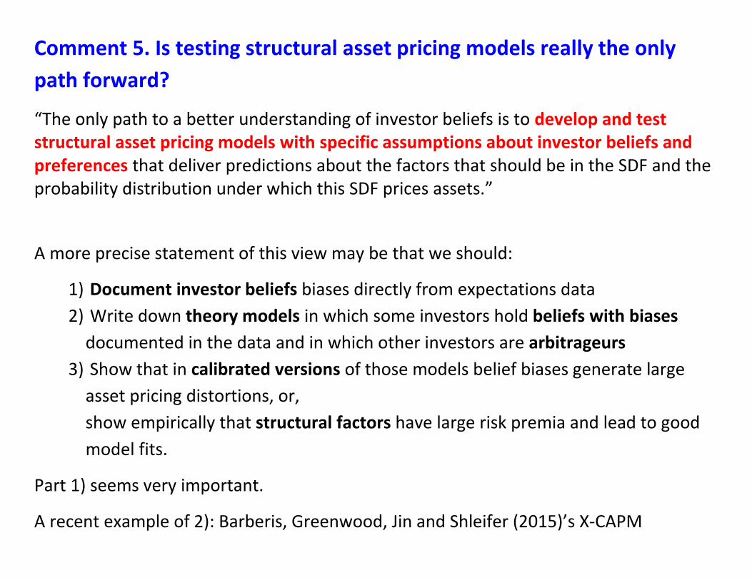
Comment 5. Is testing structural asset pricing models really the only

path forward?

“The only path to a better understanding of investor beliefs is to develop and test structural asset pricing models with specific assumptions about investor beliefs and preferences that deliver predictions about the factors that should be in the SDF and the probability distribution under which this SDF prices assets.”

A more precise statement of this view may be that we should:

1) Document investor beliefs biases directly from expectations data

2) Write down theory models in which some investors hold beliefs with biases

documented in the data and in which other investors are arbitrageurs

3) Show that in calibrated versions of those models belief biases generate large

asset pricing distortions, or,

show empirically that structural factors have large risk premia and lead to good

model fits.

Part 1) seems very important.

A recent example of 2): Barberis, Greenwood, Jin and Shleifer (2015)’s X-CAPM

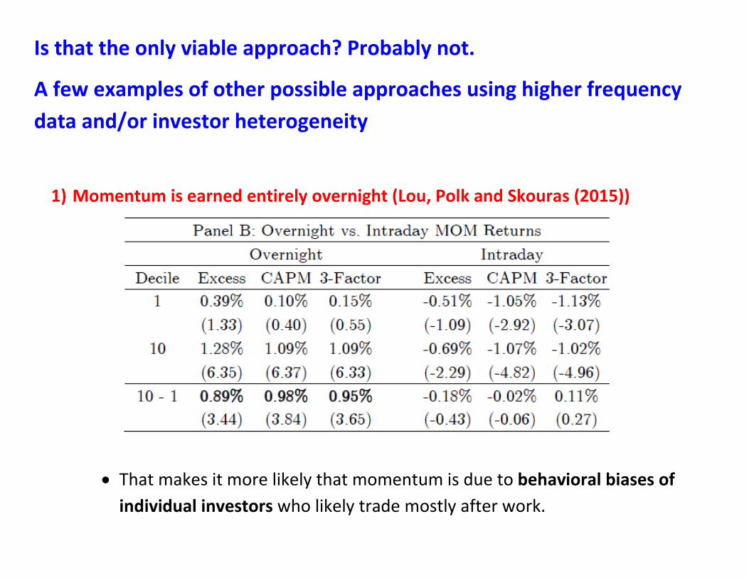
Is that the only viable approach? Probably not.

A few examples of other possible approaches using higher frequency

data and/or investor heterogeneity

1) Momentum is earned entirely overnight (Lou, Polk and Skouras (2015))

That makes it more likely that momentum is due to behavioral biases of

individual investors who likely trade mostly after work.

Consistent with that intuition, the paper shows that institutions trade against

momentum and that their institutional ownership increases area positively

correlated only with intra-day returns (and thus unlikely to be driving

momentum).

2) Investors with high human capital and high exposure to aggregate labor income

shocks tilt away from value (Betermier, Calvet and Sodini (2015))

All Swedish individuals, 1999-2007

``the patterns we uncover are overall strikingly consistent with risk-based

explanations of the value premium’’

3) The equity premium (over the past 20 years) is earned entirely in even weeks in

FOMC cycle time (Cieslak, Morse and Vissing-Jorgensen (2014))

That makes it likely that there is a large risk premium for monetary policy risk.

If so, that may move our thinking away from behavioral explanations and

towards rational models of intermediary asset pricing (since the financial sector

is leveraged about 10 to 1 and thus should be very worried about short-rate

risk).

Stock returns over the FOMC cycle, 1994-2013 Average 5-day stock return minus bill return over the FOMC cycle, percent

Based on 160 FOMC cycles (8 scheduled FOMC meetings per year). The numbers along the line indicate the value on the horizontal axis.

Note: If a given day is day -6 or closer to the next meeting, the 5-day (forward) return for this day is not used in the right part of the graph, so points to the right do not use any data for days -2 and later.

-6-6-6-6-6-6-6-6-6-6-6-6-6-6-6-6-6-6-6-6-6-6-6-6-6-6-6-6-6-6-6-6-6-6-6-6-6-6-6-6-6-6-6-6-6-6-6-6-6-6-6-6-6-6-6-6-6-6-6-6-6-6-6-6-6-6-6-6-6-6-6-6-6-6-6-6-6-6-6-6-6-6-6-6-6-6-6-6-6-6-6-6-6-6-6-6-6-6-6-6-6-6-6-6-6-6-6-6-6-6-6-6-6-6-6-6-6-6-6-6-6-6-6-6-6-6-6-6-6-6-6-6-6-6-6-6-6-6-6-6-6-6-6-6-6-6-6-6-6-6-6-6-6-6-6-6-6-6-6-6-5-5-5-5-5-5-5-5-5-5-5-5-5-5-5-5-5-5-5-5-5-5-5-5-5-5-5-5-5-5-5-5-5-5-5-5-5-5-5-5-5-5-5-5-5-5-5-5-5-5-5-5-5-5-5-5-5-5-5-5-5-5-5-5-5-5-5-5-5-5-5-5-5-5-5-5-5-5-5-5-5-5-5-5-5-5-5-5-5-5-5-5-5-5-5-5-5-5-5-5-5-5-5-5-5-5-5-5-5-5-5-5-5-5-5-5-5-5-5-5-5-5-5-5-5-5-5-5-5-5-5-5-5-5-5-5-5-5-5-5-5-5-5-5-5-5-5-5-5-5-5-5-5-5-5-5-5-5-5-5

-4-4-4-4-4-4-4-4-4-4-4-4-4-4-4-4-4-4-4-4-4-4-4-4-4-4-4-4-4-4-4-4-4-4-4-4-4-4-4-4-4-4-4-4-4-4-4-4-4-4-4-4-4-4-4-4-4-4-4-4-4-4-4-4-4-4-4-4-4-4-4-4-4-4-4-4-4-4-4-4-4-4-4-4-4-4-4-4-4-4-4-4-4-4-4-4-4-4-4-4-4-4-4-4-4-4-4-4-4-4-4-4-4-4-4-4-4-4-4-4-4-4-4-4-4-4-4-4-4-4-4-4-4-4-4-4-4-4-4-4-4-4-4-4-4-4-4-4-4-4-4-4-4-4-4-4-4-4-4-4

-3-3-3-3-3-3-3-3-3-3-3-3-3-3-3-3-3-3-3-3-3-3-3-3-3-3-3-3-3-3-3-3-3-3-3-3-3-3-3-3-3-3-3-3-3-3-3-3-3-3-3-3-3-3-3-3-3-3-3-3-3-3-3-3-3-3-3-3-3-3-3-3-3-3-3-3-3-3-3-3-3-3-3-3-3-3-3-3-3-3-3-3-3-3-3-3-3-3-3-3-3-3-3-3-3-3-3-3-3-3-3-3-3-3-3-3-3-3-3-3-3-3-3-3-3-3-3-3-3-3-3-3-3-3-3-3-3-3-3-3-3-3-3-3-3-3-3-3-3-3-3-3-3-3-3-3-3-3-3-3

-2-2-2-2-2-2-2-2-2-2-2-2-2-2-2-2-2-2-2-2-2-2-2-2-2-2-2-2-2-2-2-2-2-2-2-2-2-2-2-2-2-2-2-2-2-2-2-2-2-2-2-2-2-2-2-2-2-2-2-2-2-2-2-2-2-2-2-2-2-2-2-2-2-2-2-2-2-2-2-2-2-2-2-2-2-2-2-2-2-2-2-2-2-2-2-2-2-2-2-2-2-2-2-2-2-2-2-2-2-2-2-2-2-2-2-2-2-2-2-2-2-2-2-2-2-2-2-2-2-2-2-2-2-2-2-2-2-2-2-2-2-2-2-2-2-2-2-2-2-2-2-2-2-2-2-2-2-2-2-2

-1-1-1-1-1-1-1-1-1-1-1-1-1-1-1-1-1-1-1-1-1-1-1-1-1-1-1-1-1-1-1-1-1-1-1-1-1-1-1-1-1-1-1-1-1-1-1-1-1-1-1-1-1-1-1-1-1-1-1-1-1-1-1-1-1-1-1-1-1-1-1-1-1-1-1-1-1-1-1-1-1-1-1-1-1-1-1-1-1-1-1-1-1-1-1-1-1-1-1-1-1-1-1-1-1-1-1-1-1-1-1-1-1-1-1-1-1-1-1-1-1-1-1-1-1-1-1-1-1-1-1-1-1-1-1-1-1-1-1-1-1-1-1-1-1-1-1-1-1-1-1-1-1-1-1-1-1-1-1-1

0000000000000000000000000000000000000000000000000000000000000000000000000000000000000000000000000000000000000000000000000000000000000000000000000000000000000000

1111111111111111111111111111111111111111111111111111111111111111111111111111111111111111111111111111111111111111111111111111111111111111111111111111111111111111

22222222222222222222222222222222222222222222222222222222222222222222222222222222222222222222222222222222222222222222222222222222222222222222222222222222222222223333333333333333333333333333333333333333333333333333333333333333333333333333333333333333333333333333333333333333333333333333333333333333333333333333333333333333

4444444444444444444444444444444444444444444444444444444444444444444444444444444444444444444444444444444444444444444444444444444444444444444444444444444444444444

5555555555555555555555555555555555555555555555555555555555555555555555555555555555555555555555555555555555555555555555555555555555555555555555555555555555555555

6666666666666666666666666666666666666666666666666666666666666666666666666666666666666666666666666666666666666666666666666666666666666666666666666666666666666666

777777777777777777777777777777777777777777777777777777777777777777777777777777777777777777777777777777777777777777777777777777777777777777777777777777777777777788888888888888888888888888888888888888888888888888888888888888888888888888888888888888888888888888888888888888888888888888888888888888888888888888888888888888888

99999999999999999999999999999999999999999999999999999999999999999999999999999999999999999999999999999999999999999999999999999999999999999999999999999999999999999

10101010101010101010101010101010101010101010101010101010101010101010101010101010101010101010101010101010101010101010101010101010101010101010101010101010101010101010101010101010101010101010101010101010101010101010101010101010101010101010101010101010101010101010101010101010101010101010101010101010101010101010101010101010

11111111111111111111111111111111111111111111111111111111111111111111111111111111111111111111111111111111111111111111111111111111111111111111111111111111111111111111111111111111111111111111111111111111111111111111111111111111111111111111111111111111111111111111111111111111111111111111111111111111111111111111111111111111

12121212121212121212121212121212121212121212121212121212121212121212121212121212121212121212121212121212121212121212121212121212121212121212121212121212121212121212121212121212121212121212121212121212121212121212121212121212121212121212121212121212121212121212121212121212121212121212121212121212121212121212121212121212

13131313131313131313131313131313131313131313131313131313131313131313131313131313131313131313131313131313131313131313131313131313131313131313131313131313131313131313131313131313131313131313131313131313131313131313131313131313131313131313131313131313131313131313131313131313131313131313131313131313131313131313131313131313

14141414141414141414141414141414141414141414141414141414141414141414141414141414141414141414141414141414141414141414141414141414141414141414141414141414141414141414141414141414141414141414141414141414141414141414141414141414141414141414141414141414141414141414141414141414141414141414141414141414141414141414141414141414

15151515151515151515151515151515151515151515151515151515151515151515151515151515151515151515151515151515151515151515151515151515151515151515151515151515151515151515151515151515151515151515151515151515151515151515151515151515151515151515151515151515151515151515151515151515151515151515151515151515151515151515151515151515

16161616161616161616161616161616161616161616161616161616161616161616161616161616161616161616161616161616161616161616161616161616161616161616161616161616161616161616161616161616161616161616161616161616161616161616161616161616161616161616161616161616161616161616161616161616161616161616161616161616161616161616161616161616

17171717171717171717171717171717171717171717171717171717171717171717171717171717171717171717171717171717171717171717171717171717171717171717171717171717171717171717171717171717171717171717171717171717171717171717171717171717171717171717171717171717171717171717171717171717171717171717171717171717171717171717171717171717

1818181818181818181818181818181818181818181818181818181818181818181818181818181818181818181818181818181818181818181818181818181818181818181818181818181818181818181818181818181818181818181818181818181818181818181818181818181818181818181818181818181818181818181818181818181818181818181818181818181818181818181819191919191919191919191919191919191919191919191919191919191919191919191919191919191919191919191919191919191919191919191919191919191919191919191919191919191919191919191919191919191919191919191919191919191919191919191919191919191919191919191919191919191919191919191919191919191919191919191919

20202020202020202020202020202020202020202020202020202020202020202020202020202020202020202020202020202020202020202020202020202020202020202020202020202020202020202020202020202020202020202020202020202020202020202020202020202020202020202020202020202020202020202020202020202020202020202020202020

21212121212121212121212121212121212121212121212121212121212121212121212121212121212121212121212121212121212121212121212121212121212121212121212121212121212121212121212121212121212121212121212121212121212121212121212121212121212121212121212121212121212121212121212121212121212121212121212121

22222222222222222222222222222222222222222222222222222222222222222222222222222222222222222222222222222222222222222222222222222222222222222222222222222222222222222222222222222222222222222222222222222222222222222222222222222222222222222222222222222222222222222222222222222222222222222222

232323232323232323232323232323232323232323232323232323232323232323232323232323232323232323232323232323232323232323232323232323232323232323232323232323232323232323232323232323232323232323232323232323232323232323232323232323232323232323232323232323232323232323232323232323

2424242424242424242424242424242424242424242424242424242424242424242424242424242424242424242424242424242424242424242424242424242424242424242424242424242424242424242424242424242424242424242424242424242424242424242424

25252525252525252525252525252525252525252525252525252525252525252525252525252525252525252525252525252525252525252525252525252525252525252525252525252525252525

26262626262626262626262626262626262626262626262626262626262626262626262626262626262626262626262626262626262626262626262626262626262626262626262626262626

272727272727272727272727272727272727272727272727272727272727272727272727272727272727272727272727272727272727272727272727272727272727272727272727272727

2828282828282828282828282828282828282828282828282828282828282828282828282828282828282828282828282828282828282829292929292929292929292929292929292929292929292929292929292929292929292929303030303030303030303030303030303030303030

313131313131313131313131313131313131313131

323232323232323232323232323232323232323232

3333333333333333333333333333

-.2

0.2

.4.6

Avg

. 5-d

ay s

tock m

inu

s T

-bill

re

turn

, t to

t+

4 (

pct)

-10 0 10 20 30Days since FOMC meeting (weekends excluded)