INTERPRETING HORIZONTAL WELL FLOW PROFILES AND OPTIMIZING

WELL PERFORMANCE BY DOWNHOLE TEMPERATURE AND

PRESSURE DATA

A Dissertation

by

ZHUOYI LI

Submitted to the Office of Graduate Studies of

Texas A&M University

in partial fulfillment of the requirements for the degree of

DOCTOR OF PHILOSOPHY

December 2010

Major Subject: Petroleum Engineering

brought to you by COREView metadata, citation and similar papers at core.ac.uk

provided by Texas A&M University

INTERPRETING HORIZONTAL WELL FLOW PROFILES AND OPTIMIZING

WELL PERFORMANCE BY DOWNHOLE TEMPERATURE AND

PRESSURE DATA

A Dissertation

by

ZHUOYI LI

Submitted to the Office of Graduate Studies of

Texas A&M University

in partial fulfillment of the requirements for the degree of

DOCTOR OF PHILOSOPHY

Approved by:

Chair of Committee, Ding Zhu

Committee Members, A. Daniel Hill

Akhil Datta-Gupta

Yalchin Efendiev

Head of Department, Stephen A. Holditch

December 2010

Major Subject: Petroleum Engineering

iii

ABSTRACT

Interpreting Horizontal Well Flow Profiles and Optimizing Well Performance by

Downhole Temperature and Pressure Data. (December 2010)

Zhuoyi Li, B.E., Tsinghua University (Beijing);

M.E., Tsinghua University (Beijing)

Chair of Advisory Committee: Dr. Ding Zhu

Horizontal well temperature and pressure distributions can be measured by production

logging or downhole permanent sensors, such as fiber optic distributed temperature

sensors (DTS). Correct interpretation of temperature and pressure data can be used to

obtain downhole flow conditions, which is key information to control and optimize

horizontal well production. However, the fluid flow in the reservoir is often multiphase

and complex, which makes temperature and pressure interpretation very difficult. In

addition, the continuous measurement provides transient temperature behavior which

increases the complexity of the problem. To interpret these measured data correctly, a

comprehensive model is required.

In this study, an interpretation model is developed to predict flow profile of a

horizontal well from downhole temperature and pressure measurement. The model

consists of a wellbore model and a reservoir model. The reservoir model can handle

transient, multiphase flow and it includes a flow model and a thermal model. The

calculation of the reservoir flow model is based on the streamline simulation and the

iv

calculation of reservoir thermal model is based on the finite difference method. The

reservoir thermal model includes thermal expansion and viscous dissipation heating

which can reflect small temperature changes caused by pressure difference. We combine

the reservoir model with a horizontal well flow and temperature model as the forward

model. Based on this forward model, by making the forward calculated temperature and

pressure match the observed data, we can inverse temperature and pressure data to

downhole flow rate profiles. Two commonly used inversion methods, Levenberg-

Marquardt method and Marcov chain Monte Carlo method, are discussed in the study.

Field applications illustrate the feasibility of using this model to interpret the field

measured data and assist production optimization.

The reservoir model also reveals the relationship between temperature behavior

and reservoir permeability characteristic. The measured temperature information can

help us to characterize a reservoir when the reservoir modeling is done only with limited

information. The transient temperature information can be used in horizontal well

optimization by controlling the flow rate until favorite temperature distribution is

achieved. With temperature feedback and inflow control valves (ICVs), we developed a

procedure of using DTS data to optimize horizontal well performance. The synthetic

examples show that this method is useful at a certain level of temperature resolution and

data noise.

v

DEDICATION

To my parents, sister, and grandmother

vi

ACKNOWLEDGEMENTS

I would like to express my gratitude to my advisor Dr. Zhu for her support, guidance,

and encouragement throughout my graduate studies.

I also thank my committee members, Dr. Hill, Dr. Datta-Gupta, and Dr.

Efendiev, for their suggestion and help in my research study.

I appreciate my friends’ help too.

vii

NOMENCLATURE

A section area of the pipe

a coefficient defined in Eq. 2.40

AB coefficient defined in Eq. 2.34

AE coefficient defined in Eq. 2.34

AN coefficient defined in Eq. 2.34

AP coefficient defined in Eq. 2.34

AS coefficient defined in Eq. 2.34

AT coefficient defined in Eq. 2.34

AW coefficient defined in Eq. 2.34

B coefficient defined in Eq. 2.34

C covariance matrix

pC heat capacity

D depth

TD weight of temperature in objective function

pD weight of pressure in objective function

d observed data

e error or residual vector between observation and model calculation

wF fraction flow

f friction factor

viii

f objective function

G sensitivity matrix

g model calculated data

g gravity

H Hessian matrix

H enthalpy

aniI anisotropy ratio

I identify matrix

J Jacobian matrix

K thermal conductivity

TtK total thermal conductivity in reservoir

k permeability

dk damage permeability

ek effective permeability

rik relative permeability of phase i

l distance

M constant value to adjust damping factor

ReN Reynolds number

wNRe, wall Reynolds number

p pressure

dp pressure at damage boundary

ix

gridp average pressure in a grid

wfp flowing bottomhole pressure

hQ& heat transfer rate

q flow rate

R radius of well’s wall

dr damage radius

er effective radius

wr wellbore radius

S saturation

T temperature

IT arriving temperature

gridT grid temperature

t time

U internal energy

u Darcy velocity

V arbitrary volume

v velocity vector

v velocity

sv superficial velocity

w derivative vector

x

x parameter vector

y hold up

Z kriging function

Greek

Tα overall heat transfer coefficient

IT ,α combined overall heat transfer coefficient

β thermal expansion coefficient

γ pipe open ratio

γ semi-variogram in Chapter V

xδ upgrading parameter

θ wellbore inclination

λ kriging weight in Chapter V

µ viscosity

ρ density

probρ probability density

φ porosity

σ covariance in normal distribution

ω coefficient defined in

ϖ coefficient defined in

τ time of flight

xi

Λ kriging weight vector

Subscripts

B block in Chapter V

effe, effective

g gas

I inflow

i phase index

kji ,, position index in Appendix A

l liquid

l phase index in Appendix A

N total parameter number

n iteration step

m total observed data number

o oil

P point in Chapter V

s solid rock

w water

zyx ,, position in Appendix A

xii

TABLE OF CONTENTS

Page

ABSTRACT .................................................................................................................. iii

DEDICATION................................................................................................................ v

ACKNOWLEDGEMENTS ........................................................................................... vi

NOMENCLATURE ..................................................................................................... vii

TABLE OF CONTENTS.............................................................................................. xii

LIST OF FIGURES ..................................................................................................... xiv

LIST OF TABLES........................................................................................................ xx

CHAPTER

I INTRODUCTION............................................................................................ 1

1.1 Background .......................................................................................... 1

1.2 Literature Review ................................................................................. 2

1.2.1 Downhole Temperature Monitoring........................................... 2

1.2.2 Temperature Modeling and Interpretations ................................ 3

1.3 Objectives............................................................................................. 7

II FORWARD MODEL....................................................................................... 9

2.1 Introduction .......................................................................................... 9

2.2 Wellbore Model.................................................................................. 10

2.2.1 Wellbore Flow Model.............................................................. 10

2.2.2 Wellbore Thermal Model ........................................................ 14

2.3 Reservoir Model ................................................................................. 16

2.3.1 Streamline Simulation for Reservoir Pressure and

Saturation................................................................................ 16

2.3.2 Reservoir Thermal Model........................................................ 18

2.4 Integrated Model For Temperature at Reservoir and Wellbore

Contact ............................................................................................... 21

2.5 Solution Procedure and Model Validation........................................... 29

III INVERSION METHOD................................................................................. 33

xiii

CHAPTER Page

3.1 Levenberg-Marquardt Method ............................................................ 35

3.2 Markov Chain Monte Carlo Method ................................................... 38

3.3 Feasibility of Inversion of Temperature, Pressure and Flow ................ 40

IV RESULTS OF TEMPERATURE INTERPRETATION MODEL................... 45

4.1 Example 1: Bottom Water Driving...................................................... 45

4.1.1 Forward Model Results ........................................................... 45

4.1.2 Inversion Results..................................................................... 54

4.2 Example 2: Water Injection................................................................. 67

4.2.1 Forward Model Results ........................................................... 68

4.2.2 Inversion Results..................................................................... 73

V APPLICATIONS OF DOWNHOLE TEMPERATURE AND

PRESSURE MEASUREMENT ..................................................................... 78

5.1 Locating Gas or Water Entry in Producing Wells ................................ 79

5.1.1 Gas Entry in Oil Well .............................................................. 79

5.1.2 Water Entry in Oil Well........................................................... 84

5.1.3 Heavy Oil Well with Water Bottom......................................... 90

5.1.4 Water Entry in Gas Producing Well......................................... 95

5.2 Optimize Horizontal Well Performance by Inflow Control

Valve from Temperature Feedback ................................................... 101

5.2.1 Application Procedure of Temperature Feedback................... 103

5.2.2 Bottom Water Driving Reservoir ........................................... 107

5.2.3 Water Injection in Channel Formation................................... 122

5.3 Temperature Measurement Assists Reservoir Characterization.......... 128

5.3.1 Integrated Approach of Temperature and History

Matching............................................................................... 129

5.3.2 Downscaling Method ............................................................ 131

5.3.3 Production History Matching................................................. 136

5.3.4 Application of Approach ....................................................... 141

VI CONCLUSIONS.......................................................................................... 148

REFERENCES ........................................................................................................... 150

APPENDIX A ............................................................................................................ 156

VITA..... ..................................................................................................................... 170

xiv

LIST OF FIGURES

Page

Fig. 2.1 Differential volume element of a wellbore.................................................... 10

Fig. 2.2 Integrated temperature behavior between reservoir grid and wellbore........... 23

Fig. 2.3 Estimate formation damage effect by effective permeability......................... 28

Fig. 2.4 Calculation procedure of forward model....................................................... 29

Fig. 2.5 Linear-radial flow geometry (Furui et al., 2003) ........................................... 30

Fig. 2.6 Reservoir pressure distribution ..................................................................... 32

Fig. 2.7 Reservoir temperature distribution................................................................ 32

Fig. 3.1 Reservoir geometry information for validation case...................................... 41

Fig. 3.2 Observed and inverted pressure data at 60 days ............................................ 43

Fig. 3.3 Observed and inverted temperature data at 60 days ...................................... 43

Fig. 3.4 Observed and inverted flow rates of validation case ..................................... 44

Fig. 3.5 Inverted permeability distribution of validation case..................................... 44

Fig. 4.1 Reservoir geometry information of bottom water driving case...................... 46

Fig. 4.2 Reservoir permeability distribution and relative permeability curve.............. 46

Fig. 4.3 Oil inflow rate distribution ........................................................................... 48

Fig. 4.4 Water inflow rate distribution....................................................................... 49

Fig. 4.5 Temperature distribution in wellbore............................................................ 49

Fig. 4.6 Pressure distribution in wellbore .................................................................. 50

Fig. 4.7 Temperature derivative in wellbore .............................................................. 51

Fig. 4.8 Water cut history and transient temperature at two locations ........................ 52

Fig. 4.9 Transient wellbore temperature distribution.................................................. 53

xv

Page

Fig. 4.10 Transient arriving temperature distribution................................................... 53

Fig. 4.11 Top view of reservoir and wellbore .............................................................. 55

Fig. 4.12 Separate reservoir to sections by temperature data........................................ 56

Fig. 4.13 Objective function vs. iteration number at two initial conditions................... 57

Fig. 4.14 Matched temperature data from L-M method, homogenous initial ................ 58

Fig. 4.15 Matched pressure data from L-M method, homogenous initial ..................... 58

Fig. 4.16 Inverted oil and water flow rate profiles from L-M method,

homogenous initial ....................................................................................... 59

Fig. 4.17 Inverted permeability distribution from L-M method, homogenous

initial............................................................................................................ 60

Fig. 4.18 Matched temperature data from L-M method, 2-vlue initial.......................... 61

Fig. 4.19 Matched pressure data from L-M method, 2-vlue initial ............................... 61

Fig. 4.20 Inverted oil and water flow rate profiles from L-M method, 2-vlue initial..... 62

Fig. 4.21 Inverted permeability distribution from L-M method, 2-vlue initial .............. 63

Fig. 4.22 Objective function converges ....................................................................... 64

Fig. 4.23 Matched temperature data from MCMC method........................................... 65

Fig. 4.24 Matched pressure data from MCMC method ................................................ 65

Fig. 4.25 Inverted oil and water flow rate profiles from MCMC method ..................... 66

Fig. 4.26 Inverted permeability distribution from MCMC method............................... 67

Fig. 4.27 Reservoir geometry and well locations ......................................................... 68

Fig. 4.28 2D permeability distribution......................................................................... 69

Fig. 4.29 Oil flow rate profiles in tubing ..................................................................... 70

Fig. 4.30 Water flow rate profiles in tubing ................................................................. 70

Fig. 4.31 Wellbore temperature distribution ................................................................ 72

xvi

Page

Fig. 4.32 Wellbore pressure distribution...................................................................... 72

Fig. 4.33 Separate reservoir to sections by temperature data........................................ 73

Fig. 4.34 Matched temperature data of water injection example .................................. 74

Fig. 4.35 Temperature inverted perm vs. true perm, contour........................................ 74

Fig. 4.36 Inverted water and oil flow rate profiles of water injection example ............. 75

Fig. 4.37 Temperature inverted perm value vs. true perm average at y direction.......... 76

Fig. 4.38 Inverted water cut vs. observation ................................................................ 77

Fig. 5.1 Analysis on measured temperature ............................................................... 81

Fig. 5.2 Calculated temperature matches the measured data ...................................... 82

Fig. 5.3 Model interpretation result vs. spinner measurement .................................... 83

Fig. 5.4 Inverted permeability distribution of gas entry oil well example ................... 83

Fig. 5.5 Field measured temperature, pressure and flow rates

(Carnegie et al., 1998) .................................................................................. 84

Fig. 5.6 Use measured temperature to separate reservoir for inversion....................... 87

Fig. 5.7 Match measured temperature data of water entry oil well example ............... 88

Fig. 5.8 Match measured pressure data of water entry oil well example..................... 88

Fig. 5.9 Inverted permeability distribution of water entry oil well example ............... 89

Fig. 5.10 Model interpretation compared with production logging

measurement, oil .......................................................................................... 90

Fig. 5.11 Model interpretation compared with production logging

measurement, water...................................................................................... 90

Fig. 5.12 Match measured DTS temperature data ........................................................ 93

Fig. 5.13 Inverted permeability distribution of heavy oil well example........................ 93

Fig. 5.14 Inverted production history follows the trend of measurement...................... 94

xvii

Page

Fig. 5.15 Inverted flow rate profiles of oil and water ................................................... 95

Fig. 5.16 Measured temperature and flow meter data .................................................. 97

Fig. 5.17 Measured pressure, well trajectory and perforated locations ......................... 97

Fig. 5.18 Calculated temperature matches the trend of measured data ......................... 99

Fig. 5.19 Inverted flow rate distributions of gas and water ........................................ 100

Fig. 5.20 Inverted permeability distribution of water entry gas well example ............ 100

Fig. 5.21 Optimization procedure of operation on ICV from temperature

feedback..................................................................................................... 104

Fig. 5.22 ICV effect on pressure distribution and temperature in our model .............. 105

Fig. 5.23 Horizontal well structure ............................................................................ 108

Fig. 5.24 Reservoir geometry and 2D permeability distribution................................. 108

Fig. 5.25 Use temperature to identify high inflow rate before operating ICVs............ 109

Fig. 5.26 Flow rate profile before operating ICVs ..................................................... 109

Fig. 5.27 Choking index ratio changes in simulation at different ICV stages ............. 110

Fig. 5.28 Observe temperature feedback after controlling ICV at high

inflow section............................................................................................. 111

Fig. 5.29 Temperature achieves design at first adjustment ......................................... 112

Fig. 5.30 Inflow rate distribution at first adjustment .................................................. 113

Fig. 5.31 Second ICV operation to meet the desired temperature............................... 114

Fig. 5.32 Inflow rate is closed to evenly distribute..................................................... 114

Fig. 5.33 Daily oil rate vs. time at three conditions.................................................... 115

Fig. 5.34 Pressure at heel vs. time at three conditions................................................ 116

Fig. 5.35 Identify high inflow sections at initial, Rs = 0.05 0F ................................... 117

Fig. 5.36 Temperature achieves design, Rs = 0.05 0F................................................. 117

xviii

Page

Fig. 5.37 Unable to identify high inflow sections at 0.5 day, Rs = 0.1 0F ................... 118

Fig. 5.38 Unable to identify high inflow sections at 1 day, Rs = 0.1 0F...................... 118

Fig. 5.39 May identify high inflow sections at 2 days, Rs = 0.1 0F............................. 119

Fig. 5.40 Identify high inflow sections at initial, σ = 0.033 0F ................................... 120

Fig. 5.41 Temperature achieves design, σ = 0.033 0F................................................. 120

Fig. 5.42 Failure to identify high inflow sections at 0.5 day, σ = 0.1 0F ..................... 121

Fig. 5.43 Failure to identify high inflow sections at 5 day, σ = 0.1 0F ........................ 121

Fig. 5.44 Reservoir geometry and 2D permeability distribution used in

example 2................................................................................................... 123

Fig. 5.45 Use temperature to identify inflow rate distribution.................................... 124

Fig. 5.46 Inflow rate distribution before operating ICV............................................. 124

Fig. 5.47 Choking index ratio changes along wellbore .............................................. 125

Fig. 5.48 Temperature after ICV operation................................................................ 126

Fig. 5.49 Inflow rate distribution after ICV operation................................................ 126

Fig. 5.50 Daily oil rate shows the production improvement ....................................... 127

Fig. 5.51 Integrated approach for incorporating temperature data into history

matching .................................................................................................... 131

Fig. 5.52 Downscaling of the temperature inverted coarse-scale permeability ........... 132

Fig. 5.53 Simple example for kriging estimation ....................................................... 132

Fig. 5.54 Illustration of generalized travel time difference and correlation

function (Cheng et al., 2004) ...................................................................... 137

Fig. 5.55 A sample of generated permeability fields from the integrated approach .... 142

Fig. 5.56 Calculated water-cut history matches observation....................................... 143

Fig. 5.57 Calculated temperature matches observation .............................................. 143

xix

Page

Fig. 5.58 Inverted flow rate profiles in tubing for oil and water ................................. 144

Fig. 5.59 Matching water-cut history......................................................................... 145

Fig. 5.60 Permeability distributions derived from water cut and well data only ......... 145

Fig. 5.61 Calculated temperature fails to match observation ...................................... 146

Fig. 5.62 Downhole flow rates may not be predicted correctly by history

matching only ............................................................................................ 147

xx

LIST OF TABLES

Page

Table 2.1 Fluid Properties in Program Validation...................................................... 31

Table 2.2 Reservoir Parameters in Program Validation.............................................. 31

Table 3.1 Reservoir and Well Parameters in Program Validation............................... 41

Table 3.2 Fluid and Rock Properties.......................................................................... 42

Table 4.1 Input for Reservoir and Wellbore of Water Driving Example..................... 47

Table 4.2 Input for Reservoir and Wellbore of Water Injection Example................... 69

Table 5.1 Input for Reservoir and Wellbore of Gas Entry in Oil Well Example ......... 80

Table 5.2 Input for Reservoir and Wellbore of Water Entry Oil Well Example.......... 86

Table 5.3 Input for Reservoir and Wellbore of Heavy Oil Well Example .................. 92

Table 5.4 Input for Reservoir and Wellbore of Water Entry Gas Well Example......... 98

1

1 CHAPTER I

INTRODUCTION

1.1 BACKGROUND

Horizontal well technology has been widely used to obtain larger contact between

wellbore and reservoir. Downhole flow conditions of horizontal well in general are

complicate because of a large degree of reservoir heterogeneity being involved

compared with vertical wells. With correct understanding of downhole flow conditions,

well operation may be applied to improve production, for example, unwanted fluid can

be constrained to enter the wellbore. Therefore, diagnosis of horizontal well downhole

flow conditions has important impact on production optimization.

One of the commonly used methods to obtain downhole flow conditions is

production logging. Spinner flowmeter is one of the most popular conventional ways to

generate downhole flow distributions. Profiles of fluid velocities in a well can be

obtained by interpreting spinner flowmeter responses. However, in multiphase flow

horizontal well, because the well is horizontal, phases will be segregated by gravity.

Therefore, spinner flowmeter may involve higher-level of error, and it is hard to identify

individual phase flux.

Temperature and pressure data are generally measured during a conventional

production logging. Recently, advanced technology, such as distributed temperature

sensor (DTS) and downhole permanent pressure sensor, have been installed in horizontal

This dissertation follows the style of SPE Journal.

2

wells as a part of well completion. This new technology provides us continuous

downhole temperature and pressure data with certain accuracy. It is possible to reveal

the downhole flow conditions from interpretation of measured temperature and pressure

data.

For horizontal wells, because geothermal temperature changes are relatively

small, the dominating effects on the wellbore temperature changes may be thermal

expansion, viscous dissipative heating, and thermal conduction. Model for temperature

interpretation should be able to handle these subtle thermal effects. These features post

additional challenges to methodology development. Over-simplified model will not

provide useful information, but too detailed model will result in interpretation

difficulties.

1.2 LITERATURE REVIEW

1.2.1 Downhole Temperature Monitoring

Temperature log has been used to evaluate production profiles and problems in the

industry, such as detecting water or gas entries, locating casing leaks, identifying

injection or production zones (Hill, 1990). As a standard practice of production and

diagnosis, production has to be disturbed. When running production logging, it is costly

and time consuming, and it is only provides periodical information while logging.

Sometimes the information strongly depends on well completions and trajectory,

especially for horizontal well.

3

Currently, new techniques, such as distributed temperature sensor (DTS), have

been used to achieve real-time monitoring. Its applications are broad. Foucault et al.

(2004) used DTS data to detect the water entry location at a horizontal well. Fryer et al.

(2005) monitored the real time temperature profiles to identify and correlate production

changes for the well in multizone reservoir. Johnson et al. (2006) and Huebsch et al.

(2008) calculated gas flow profiles from the measured DTS data. Julian et al. (2007)

showed that DTS data can be used to determine the leak location in vertical wells.

Huckabee (2009) applied the DTS data to diagnose the fracture stimulation and evaluate

well performance.

DTS technology has shown its great potential of production evaluation.

However, temperature data is qualitatively analyzed in most of these previous works.

Quantitative interpretation of the temperature data can provide more useful information

for understanding the downhole flow condition, adding invaluable benefit to production

monitoring and optimization.

1.2.2 Temperature Modeling and Interpretations

One of the earliest works on temperature modeling was proposed by Ramey (1962).

Ramey’s model can be applied to predict temperature profiles for injection or production

wells with only single phase flowing. In this model, no inflow or outflow between the

wellbore and the formation, temperature in well is a function of time and depth. The heat

conducted radially from the casing to the formation is transient. A time-dependent

function is introduced, which is a log linear solution of time, thermal diffusivity, and

4

radius of outside casing, and depends on the boundary condition assumed for the heat

conduction between formation and wellbore.

Satter (1965) modified Ramey’s model for steam injection wells by including

phase changes. Sagar et al. (1991) extended Ramey’s equation to inclined wells, and

considered Joule-Thomson effect caused by pressure change along the wellbore. Hasan

and Kabir (1994) further developed Ramey’s model. They provided an approximate

solution of the time-dependent function based on a detailed thermal conduction model of

the formation. They also considered the Joule-Thomson effect in the wellbore, and the

model can handle two-phase flow. All of the above models assume that there is no fluid

transport between wellbore and formation.

To study the transient thermal behavior and allow fluids to entry into the

wellbore from different locations along the wellbore, new temperature models were

developed. Kabir et al. (1996) derived a detailed wellbore model based on mass,

momentum and energy balance. The arriving temperature which implies the inflow fluid

temperature at the boundary of outside the wellbore and the reservoir is assumed to be

the geothermal temperature. One advantage of this model is that it accounts the tubular

heat absorption or the thermal storage effect, which is observed during well testing.

Izgec et al. (2006) developed a coupled wellbore/reservoir model for transient fluid and

heat flow. In their work, they also assume the arriving temperature is equal to the

reservoir geothermal temperature. These works are based on the assumption that fluid

flow in the well is single-phase flow.

5

For vertical or inclined wells, the well temperature change is dominated by heat

transfer between the wellbore fluid and the formation. Because of geothermal gradient,

formation temperature along the depth of the wellbore changes significantly. At such a

situation, some small thermal effects, such as fluid thermal expansion and viscous

dissipation heating, can be ignored compared with the heat transfer caused by fluids flow

from the formation to the wellbore. Therefore, the above models have been applied in

the field. However, for horizontal wells, the geothermal temperature change is very

small. At this condition, these small thermal effects become important. We can imagine

that if assuming the arriving temperature is equal to geothermal temperature and

ignoring the pressure change along the horizontal well, the temperature distribution in a

horizontal well should be close to a constant. Many field observations (Carnegie et al.,

1998; Chace et al., 2000; Foucault et al., 2004; Heddleston, 2009) showed that

temperature distributions in horizontal wells changes along the wellbore, which is not

caused by the geothermal temperature. These field measured data indicate that small

thermal effects of fluids from formation to wellbore should be included in a more precise

thermal model when coupling the well and the reservoir model for horizontal wells.

The early work including these small thermal effects is proposed by Maubeuge

et al. (1994). Their reservoir thermal model numerically solves a transient temperature

equation which includes thermal expansion and viscous dissipation. However, their

wellbore model is not explained clearly in their paper.

Because the DTS technique has been used increasingly, many temperature

models (Ouyang and Belanger, 2006; Pinzon et al., 2007; Wang et al., 2008; Yoshioka et

6

al., 2005; Yoshioka et al., 2007b) have been developed to interpret the DTS data for

vertical, inclined or horizontal wells. The significant improvement of these models is

that they include subtle thermal changes in the reservoir for multiphase flow wells,

comparing with conventional reservoir thermal model used in thermal flooding. These

models still assume that the flow in the wellbore is steady state. Most of them assume

the arriving temperature is equal to geothermal temperature plus the Joule Thomson

effect, and the pressure used to calculate Joule Thomson effect is equal to average

drawdown pressure. In Pinson’s work, they pointed out that the relation overestimates

the temperature change. This was also noticed by Brady et al. (1998) who used half of

the pressure drawdown to calculate the Joule Thomson effect. In Yoshioka’s model, the

reservoir model is segmented into finite pieces. Over each segment, the flow is single

phase, steady sate flow, and the temperature does not change with time. Analytical

solution of reservoir flow was used to describe the pressure and flow relationship, and

the arriving temperature is analytically solved.

Besides these steady state models, Duru and Horne (2008), and Sui et al. (Sui et

al., 2008b) developed thermal models that consist of both a transient wellbore model and

a transient reservoir model. The well models are mainly used for vertical wells, and

radial flow assumption is used in the reservoir models. Sui’s work also showed that the

transient well model can be reduced to steady state condition if observed time is long

enough, for example, days (Sui, 2009).

Based on these models, measured temperature data can be interpreted for

different applications, such as diagnosing downhole flow rate profiles, detecting water

7

entry, and determining reservoir and formation damage permeabilities. Generally, the

interpretation is based on a forward thermal model and an inversion method to minimize

the least-square difference between the forward calculated result and the observed data.

Sui et al. (2008a), and Yoshioka et al. (2007a) used the standard gradient based method,

Levenberg-Marquardt method, in their inversion, and Donovan et al. (2008) used a

probalistic production model for their temperature interpretation. All of these results

proved the success of temperature data applications in analyzing wellbore downhole

conditions.

Additionally, inflow control valves (ICV) are increasingly used in horizontal

wells. These equipments can regulate the inflow fluid for horizontal wells, which may

optimize production. Alhuthali et al. (2007) proposed a rate control method to obtain

uniform travel time based on streamline method. This method is based on known

geology characteristic of the reservoir. For unknown geology characteristic, operating

the ICVs based on this method requires other information, such as measured

temperature, to analysis whether the operation of ICVs achieves the design of the

controlling rate.

1.3 OBJECTIVES

The objective of this study is to interpret measured temperature and pressure data to

downhole flow conditions in horizontal wells for completely transient flow conditions.

The interpretation is based on a detailed thermal model. Though numerous wellbore

models are developed, the reservoir models coupled with the wellbore models still have

8

limitations. For transient, multiphase flow in horizontal wells, the coupled reservoir

model for temperature interpretation should have functions to predict complex flows,

and accounts for subtle thermal effects of fluid thermal expansion and viscous

dissipation heating when fluid flows from the reservoir to the wellbore.

In this study, we first develop a transient, multiphase flow, 3D reservoir model

based on streamline simulation for reservoir flow calculation and finite difference

method for temperature calculation. The reservoir thermal model includes thermal

expansion and viscous dissipation heating. Then we obtain a forward model by

integrating the reservoir model and a previous published well model (Yoshioka et al,

2005). Although the wellbore thermal model is under steady state assumption,

temperature was updated at each time step sequentially after solving the reservoir

temperature.

From the forward model, we invert observed temperature and pressure data to

flow rate profiles by using inversion methods. We also apply this model to field

applications, use temperature data to generate reservoir characteristics, and optimize

intelligent horizontal well performance by monitoring real time temperature feedback

with a rate control method. The results shown in this study illustrates how temperature

data can help to monitor, control and optimize oil and gas production.

9

2 CHAPTER II

FORWARD MODEL

2.1 INTRODUCTION

In this chapter, we develop a forward model to predict downhole temperature, pressure

and flow rate profiles for horizontal wells. The forward model consists of a wellbore

model and a reservoir model.

The wellbore model is a steady state model. It includes a wellbore flow model

calculating pressure and fluid velocity distributions along wellbore, and a wellbore

thermal model solving the wellbore temperature distribution. The model includes

detailed heat transfer mechanism to predict wellbore temperature.

The reservoir model is a transient, multiphase flow, 3D model which is based on

streamline simulation for reservoir flow calculation and finite difference method for

temperature calculation. The reservoir thermal model includes thermal expansion and

viscous dissipation heating which can reflect small temperature changes caused by

pressure difference. At each time step, the wellbore temperature is updated based on the

reservoir temperature to count on the temperature change as a function of time.

All of the wellbore model equations and the reservoir model equations are

discretized to solve by numerical simulation. An integrated model is developed to couple

temperature behavior at the contact between the wellbore and the reservoir. Combing the

wellbore model, the reservoir model, and the integrated model, we can obtain transient

10

pressure, temperature, and flow rate profiles along wellbore by applying appropriate

initial and boundary conditions.

2.2 WELLBORE MODEL

The model developed by Yoshioka et al. (2005, 2007b) was adopted directly in this

study. Fig. 2.1 shows a differential volume element of a wellbore, and the reservoir fluid

flows into the well through the wall of wellbore. Wellbore flow and thermal behaviors

are steady state.

Fig. 2.1 Differential volume element of a wellbore

2.2.1 Wellbore Flow Model

The velocities in wellbore and at the wall of well are represented by:

11

Rr

v

v

v

v

v

I

r

x

=

=

=

wallswell'at

wellborein

0

0

0

0

θ

v ................................................................. (2.1)

where v is the velocity vector and the subscript I means arriving. Fig. 2.1 illustrates the

velocity component in the system. In the wellbore, the velocity vector in wellbore has

only one component at axial (x) direction, and the arriving velocity vector at well’s wall

(r=R) has only one component at radial (r) direction.

Mass Balance

Considering the fluid flows from reservoir into wellbore, the mass balance equation for

each phase is

( )( )

iIIi v

Rdx

vydρ

γρ 2= .................................................................................... (2.2)

where the subscript i is the type of fluid phase, which could be oil, gas, or water. And γ

is the ratio of the opening section versus the total well length. For an open hole

completion, γ =1. And if the well is partially open to the reservoir though completion,

the γ is less than one.

Momentum Balance

Using the momentum balance, the pressure equation can be obtained as follows:

12

( )θρ

ρρsin

22

gdx

vd

R

fv

dx

dpm

mmmm −−−= ........................................................ (2.3)

where the subscript m denotes the mixed multi-phase fluids, and f is friction factor. For

horizontal wells, Ouyang et al. (1998) has presented a friction factor model which states:

for laminar flow, the friction factor is independent of completion type and is calculated

by:

( )( )6142.0

Re,

Re

04304.0116

wN

Nf += .................................................................. (2.4)

For turbulence flow, friction factor is affected by different completion types,

( )( )

−

−

=

wellperforated

completionopenhole

0153.01

03.291

3978.0

Re,0

8003.0

Re

Re,

0

w

w

Nf

N

Nf

f ......................... (2.5)

where ReN and wNRe, are the Reynolds number and the wall Reynolds number. Their

definitions are

µ

ρvRN

2Re = ................................................................................................. (2.6)

and

I

IIw

vRN

µ

ρ2Re, = ............................................................................................ (2.7)

0f is the friction factor without radial influx and is calculated from Moody’s diagram or

from Chen’s correlation (Chen, 1979):

13

28981.0

Re

1098.1

Re

0

149.7

7065.3log

0452.5

7065.3log4

−

+−−=

NNf

εε.................... (2.8)

where ε is the relative roughness of the pipe.

For multiphase flow conditions, we need to calculate average density and

velocity to solve Eq. 2.3. When the flow is oil-water two-phase flow, we assume no slip

between phases, and then the mixed velocity can be expressed

sw

m

wso

m

om vvv

ρ

ρ

ρ

ρ+= .................................................................................... (2.9)

where swv and sov represent superficial velocities of water and oil. The oil-water mixture

viscosity is estimated by a correlation (Jayawardena et al., 2000):

( ) 5.21

−−=

dcmyµµ ........................................................................................ (2.10)

where the subscript c means continuous phase, d means dispersed phase, and d

y is the

holdup of dispersed phase.

When the flow is gas-liquid multi-phase flow, the drift flux model (Ouyang and

Aziz, 2000) is used to estimate the pressure gradient. Its final expression (Yoshioka,

2007) is

( )

−+

+−−

−=

21

2

1sin1

1

aWaW

m

mm

dx

dp

dx

dpg

R

fv

dx

dpϖϖθρ

ρ

χ................ (2.11)

where

14

( )p

vvv

sg

sggsll ρρχ += ................................................................................... (2.12)

( )( ) ( )( )[ ]gIlIsggsllgIglIlsgsl

aW

vvvvvvvvAdx

dp,,,,

1

1+++++−=

ρρρρ ........... (2.13)

and

( )( )gIglIlsggsll

maW

vvvvAdx

dp,,

2

2ρρρρ

ρ++−=

......................................... (2.14)

Eq. 2.13 and Eq. 2.14 account for the accelation pressure drop casued by wall influx.

The subscript s denotes surperficial, l denotes liquid, g denotes gas, A is the section area

of the pipe. The value of ϖ is proposed as 0.8 by Ouyang and Aziz (2000).

2.2.2 Wellbore Thermal Model

Wellbore temperature equation is derived from energy balance. It is assumed that the

temperature in horizontal well is 1D, steady state. Kinetic energy and viscous shear are

ignored because they almost do not affect temperature profiles. The final formulation of

temperature in wellbore is:

( )( ) ( ) ( ) ( )

( ) θρ

ρ

ρ

α

ρ

ρsin

2 ,g

vC

vTT

vCRdx

dp

vC

KvC

dx

dT

Tp

TI

Tp

IT

Tp

TJTp−−+= ....................... (2.15)

where

15

( ) ( ) TITpIT vC αγργα −+= 1,, ........................................................................ (2.16)

( ) ∑=i

iiiT yvv ρρ ......................................................................................... (2.17)

( ) ∑=i

ipiiiTp CyvvC ,ρρ ............................................................................... (2.18)

and

( ) ∑=i

iJTipiiiTJTp KCyvKvC ,,ρρ ................................................................. (2.19)

the subscript T means total fluid phases in the flow, and Tα denotes the overall heat

transfer coefficient.

The full formulation of Tα was originally presented by Willhite (1967), which

includes the heat convection between flowing fluid and inside wall of tubing, heat

conduction in tubing wall, casing, and cement, and conduction, natural heat convection,

and radiation in annulus between tubing and casing.

In this study, the temperature change in horizontal wells is very small, so we

can ignore the natural heat convection and radiation in annulus. Fluid flow in tubing is

usually at relatively high Reynolds number, so the thermal resistance by heat convection

between flowing fluid and inside wall of tubing can be ignored. And because steel has

high thermal conductivity, the thermal resistance of tubing and casing are negligible.

Therefore, to calculate Tα , we use a reduced equation presented by Sagar et al. (1991):

16

1

sin

sinlnln

−

−−

−

−

+=cement

ODgca

w

annulus

ODtubing

IDgca

IDtubingTK

r

r

K

r

r

rα ............................................... (2.20)

Thus, the overall heat transfer coefficient is constant if the completion structure of a well

is specified.

Because the wellbore mass, pressure, and temperature equations are all non-

linear equations, they are discretized with a finite difference scheme and solved by

numerical simulation.

2.3 RESERVOIR MODEL

In this section, we introduce the reservoir model, which is a transient, multiphase flow,

3D model. The model is based on streamline simulation for reservoir flow calculation

and finite difference method for temperature calculation. The reservoir thermal model

includes thermal expansion and viscous dissipation heating.

2.3.1 Streamline Simulation for Reservoir Pressure and Saturation

A parallelepiped shaped reservoir is used to develop the reservoir flow and thermal

model. For reservoir flow, we use the streamline simulation method (Datta-Gupta and

King, 2007; Pollock, 1988) to solve the reservoir pressure and saturation distribution.

The streamline simulation is a black oil simulation model that uses mass conservation

equation for each phase:

17

( ) ( ) 0=⋅∇+∂

∂iiii

uSt

vρφρ .............................................................................. (2.21)

and the velocity follows Darcy’s law

( )gpk

uv

vvv

ρµ

+∇⋅−= ........................................................................................ (2.22)

Streamline is formed based on the velocity field, and the phase saturation is solved

along the streamline space. The saturation equation for two-phase slightly compressible

fluid in streamline time of flight coordinate is

0=∂

∂+

∂

∂

τww

F

t

S............................................................................................. (2.23)

where

ξφ

τ du∫

=0

v ..................................................................................................... (2.24)

is the time of flight, and the fractional flow, w

F , is

orowrw

wrw

wkk

kF

µµ

µ

//

/

+= ................................................................................ (2.25)

where r

k is relative permeability and µ is viscosity. Neglecting the viscosity change,

wF is only a function of saturation.

In this work, a numerical simulation (FrontSim, 2008) was used to obtain the

solution of the above equations.

18

2.3.2 Reservoir Thermal Model

For an arbitrary volume V in reservoir, the energy conservation equation can be

expressed as,

+

=

VVV in

production

energy of Rate

into

nsportenergy tra

of rateNet

in

energy of rate

onAccumulati

......................... (2.26)

Neglecting the kinetic energy change, the accumulation rate in V is (Lake, 1989)

( ) ( ) VUgDUS

V

dtt

tissiii ⋅

∑ −++=

+

ρφρφ 1

in

energy of rate

onAccumulati

....................... (2.27)

where the subscript i denotes fluid phase, s is solid rock, U is the internal energy, D is

the depth, and S is the saturation.

The energy transport includes convection,

( ) A

into

nsportenergy tra

of Convection

⋅+=

∑i

iii gDHu

V

vρ ................................................... (2.28)

and conduction

( ) A

into

nsportenergy tra

of Conduction

⋅∇−=

TK

V

Tt .............................................................. (2.29)

where H is the enthalpy, and Tt

K is the total heat conductivity, and A is the surface area

of the arbitrary volume V.

19

For the arbitrary volume V in reservoir without a wellbore, the rate of energy

production is zero. Substituting Eq. 2.27 through Eq. 2.29 into Eq. 2.26, the reservoir

energy conservation can be expressed as

( ) ( )

( ) ( )TKgDHu

UgDUSt

Tt

i

iii

i

ssiii

∇⋅∇−

+⋅∇=

−++

∂

∂−

∑

∑

vρ

ρφρφ 1

........................................... (2.30)

From the definition of enthalpy and internal energy,

dpTdTCdH p )1(1

βρ

−+= ........................................................................... (2.31)

and

ρpHU −= ................................................................................................ (2.32)

and we assume that for the formation rock

dTCdU pss ≈ ................................................................................................ (2.33)

Then substituting Eq. 2.31 through Eq. 2.33 into Eq. 2.30, and rearranging it, we

can obtain the temperature equation in reservoir as follows:

( ) ( )

( )

( ) ( )∑∑

∑∑

∑∑

∇⋅+∇⋅−

∇⋅+∇⋅∇−∇⋅=

∂

∂+

∂

∂

−+−

i

ii

i

iii

i

iiTt

i

piii

i

iiipss

i

piii

gDupuT

puTKTCu

t

pTS

t

TCCS

vv

vv

ρβ

ρ

βφρφρφ 1

.................................. (2.34)

On the left hand side of Eq. 2.34, the first term is the accumulative term, and the second

term is a thermal expansion term related to transient pressure change. On the right hand

side, the first term is the convection term, the second term is the conduction term, the

20

third one is the viscous dissipation heating, the fourth one is the thermal expansion

because of pressure change, and the last term is related to potential energy.

TtK is the total heat conductivity and its change is not significant. Therefore, it

is treated as a constant in this work.

We use the finite difference method to solve the temperature equation

numerically. If it is no specified, the top and bottom boundaries are assigned a constant

temperature, and all the other reservoir boundaries are set equal to geothermal

distributed temperature. Only for water injection cases, two parallel horizontal wells are

set near reservoir boundaries, and it is assumed no heat flux at the boundary.

To solve Eq. 2.34, we apply finite difference scheme to discretize the equation.

The general form for this discretized equation is:

kji

n

kjikji

n

kjikji

n

kjikji

n

kjikji

n

kjikji

n

kjikji

n

kjikji

BTATTABTAN

TASTAETAWTAP

,,

1

1,,,,

1

1,,,,

1

,1,,,

1

,1,,,

1

,,1,,

1

,,1,,

1

,,,,

++++

++=

++

+−

++

+−

++

+−

+

........................... (2.35)

The detailed procedure of discretization and coefficients in Eq. 2.35 can be found in

Appendix A.

In the numerical simulation, if a reservoir grid has a wellbore segment in it,

then its temperature equation, Eq. 2.30, should include the heat transfer between the grid

and the wellbore segment into the right hand side. The heat transfer term is

( ) ( )Ires

iip

rr

Ttwellres

hTTCu

r

TKQ

w

−⋅+∂

∂−= ∑

=−

v& ρ ........................................ (2.36)

In this work, the reservoir temperature change is relatively small, so it is

assumed that the fluid properties are not affected by temperature change, which implies

21

that the temperature solution has no influence on the pressure and saturation solution. To

couple the pressure, saturation and temperature in numerical simulation, the pressure

discretized equation was solved first. Then fluxes were solved from the Darcy’s law, and

used total velocity tracing 1D streamline. Along streamlines we can calculate saturations

based on Eq. 2.23. After that, the saturation in grid is averaged calculated from

streamlines to their passing grids. With the pressure and saturation fields, the

temperature equation is then solved. For pressure and temperature fields, it uses the same

time step for update, which should guarantee that it does not change general streamline

pattern, e.g., total time of fight along streamlines do not vary more than 5% (if fail,

reduce the time step).

2.4 INTEGRATED MODEL FOR TEMPERATURE AT RESERVOIR AND

WELLBORE CONTACT

To solve temperature equations, Eq. 2.15 and Eq. 2.30, we must know the arriving

temperatureI

T , which is the link between reservoir grid temperature and wellbore

temperature. The following assumptions have been made to solve I

T :

1. Reservoir grid temperature and pressure are located at the effective radius, effr ,

which follows the definition of Peaceman’s model (Peaceman, 1983):

22

25.025.0

5.0

2

5.0

2

5.0

28.0

+

∆⋅

+∆⋅

=

z

y

y

z

z

y

y

z

eff

k

k

k

k

zk

ky

k

k

r ................................................. (2.37)

2. The permeability is isotropic and homogenous in reservoir grid, which is given

by

( ) 5.0

zye kkk ⋅= .............................................................................................. (2.38)

3. Fluid flow from the effective radius to the wellbore is radial flow.

4. In one time step, both the pressure and temperature are assumed at steady state.

5. Because the distance from the grid to wellbore is very small, the fluid properties

and saturation are treated as constant

6. Effects of capillary pressure and gravity are ignored.

For the grid contains a well in it, Fig. 2.2 illustrates the thermal/flow system

used in this work.

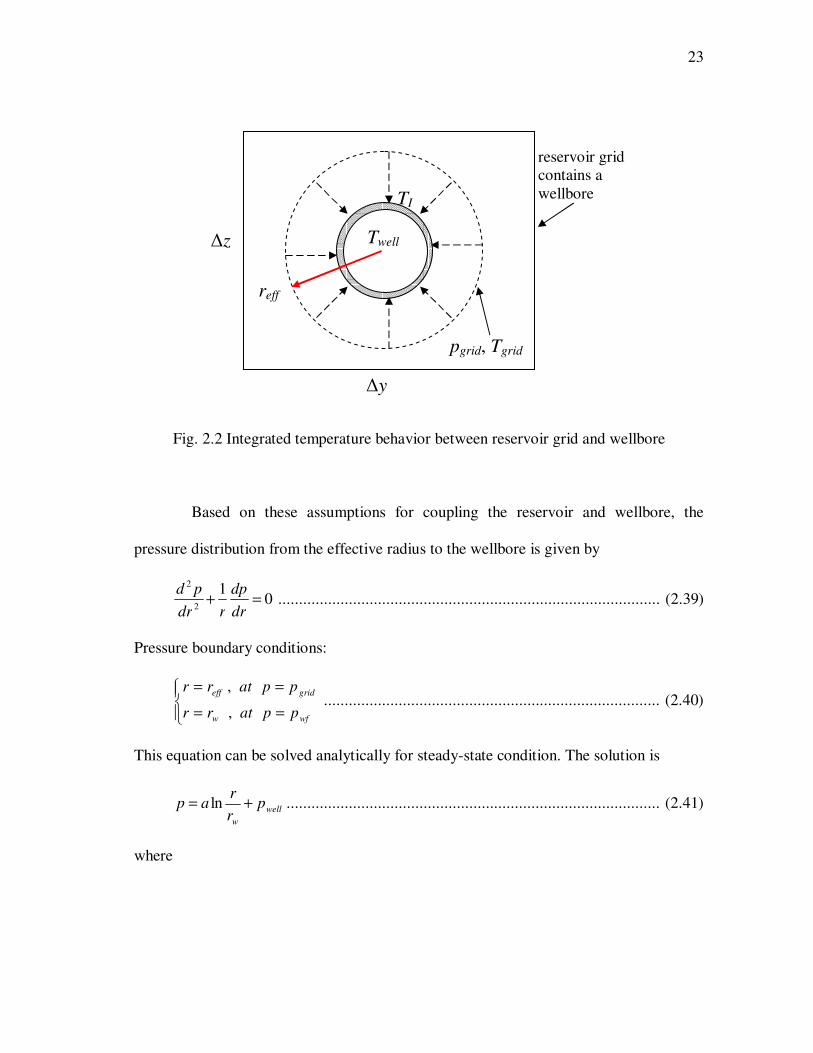
23

Fig. 2.2 Integrated temperature behavior between reservoir grid and wellbore

Based on these assumptions for coupling the reservoir and wellbore, the

pressure distribution from the effective radius to the wellbore is given by

01

2

2

=+dr

dp

rdr

pd............................................................................................ (2.39)

Pressure boundary conditions:

==

==

wfw

grideff

ppatrr

ppatrr

,

,................................................................................. (2.40)

This equation can be solved analytically for steady-state condition. The solution is

well

w

pr

rap += ln .......................................................................................... (2.41)

where

∆z

∆y

pgrid, Tgrid

TI

Twell

reff

reservoir grid

contains a

wellbore

24

( )weff

wfgrid

rr

ppa

ln

−= ............................................................................................. (2.42)

The equation described temperature distribution from the reservoir grid to the wellbore

outside is

( ) ( ) ( ) 01

=

−++ ∑∑∑

dr

dTr

dr

d

rK

dr

dpu

dr

dpTu

dr

dTuC Tt

i

ri

i

rii

i

ripii βρ .............. (2.43)

The first term is convection term, the combination of the second and third term is

viscous dissipation heating, and the fourth term is the conduction term.

The boundary conditions for the temperature equation are:

( )

=−=

==

==

wwrrT

Rr

Tt

effgrid

rratTTdr

dTK

rratTT

w

,

,

α............................................... (2.44)

First, we get the velocity from Darcy’s law for each phase:

r

akk

dr

dpkku

i

rie

i

rieri

µµ−=−= ............................................................................ (2.45)

Substituting Eq. 2.41, Eq. 2.42, and Eq. 2.45 into Eq. 2.43, and rearranging it, we get a

second order partial differential equation of temperature only:

011

1

2

2

2

2

=

−

+

+

∑

∑∑

dr

dTr

dr

d

rK

rka

k

r

Tka

k

dr

dT

rak

kC

Tt

i

e

i

ri

i

e

i

rii

i

e

i

ripii

µ

µβ

µρ

.................................... (2.46)

Because we assume the fluid properties and saturation are constant in one time step, Eq.

2.46 can be simplified as

25

03212

22 =+++− CTC

dr

dTrC

dr

TdrKTt ........................................................... (2.47)

where

∑

∑

∑

=

=

−

=

i

e

i

ri

i

e

i

ri

i

i

Tte

i

ri

pii

kak

C

kak

C

Kakk

CC

2

3

2

2

1

,

µ

µβ

µρ

................................................................... (2.48)

are treated as constant. Solution for this second-order differential equation is

brcrcTnn ++= 21

21 ...................................................................................... (2.49)

where

∑

++

−=

i

i

i

ri

Tt

e k

K

akn β

µω

ω 22

1 42

1

2........................................................... (2.50)

∑

+−

−=

i

i

i

ri

Tt

e k

K

akn β

µω

ω 22

2 42

1

2.......................................................... (2.51)

( ) ( )

1221

22

21

2

1

n

eff

n

w

Tt

T

w

n

eff

n

w

Tt

T

w

grid

n

w

Tt

T

w

w

Tt

Tn

eff

rrKr

nrr

Kr

n

bTrKr

nTb

Kr

c

−−

−

−

−−−

=αα

αα

.............................................. (2.52)

( ) ( )

1221

11

21

1

2

n

eff

n

w

Tt

T

w

n

eff

n

w

Tt

T

w

w

Tt

Tn

effgrid

n

w

Tt

T

w

rrKr

nrr

Kr

n

TbK

rbTrKr

n

c

−−

−

−−−

−

=αα

αα

............................................... (2.53)

26

Tt

e

i i

ripii

K

akkC∑

=

µρω .............................................................................. (2.54)

and

∑

∑

=

i

i

i

ri

i i

ri

k

k

b

βµ

µ......................................................................................... (2.55)

For the arriving temperaturewrrI TT

== , just substitute wrr = into Eq. 2.49.

According to these equations, reservoir grid, arriving temperature, and wellbore

temperature are coupled together. To uncouple them and reduce the numerical

simulation time without losing significant accuracy, we use explicit scheme to estimate

the heat transfer term for reservoir grid. Arriving temperature IT and wellbore

temperature wT are implicit. We iteratively solve the wellbore temperature Eq. 2.15 and

the integrated temperature Eq. 2.49, until the solution reaches convergence.

During drilling, completion, and production, formation damage may occur,

which will increase the pressure drop for a given flow rate. This change of pressure

behavior can affect temperature behaviors. One possible way to account formation

damage effect is to use small grid to catch the damage range. However, generally the

formation damage range is very small, and small grid requires small time step to satisfy

the numerical stability.

Another way to handle formation damage is to keep the same grid distribution,

but use a new effective permeability to estimate formation damage. Assume the

27

formation damage is radial range with permeability dk and radius dr , as shown in Fig.

2.3. Peaceman effective radius effr ( deff rr > ) and effective permeability ek are still

calculated by Eq. 2.37 and Eq. 2.38 respectively. The flow from reservoir grid to outside

damage range is radial flow, and the flow from outside damage to wellbore is also radial

flow. The pressure at outside damage, dr , is dp . Thus, the flow rate from the grid to the

wellbore at the defined boundary condition is:

( ) ( )

w

d

wdd

d

eff

dgride

r

r

ppxk

r

r

ppxkq

lnln

1

µµ

−∆=

−∆= ........................................................ (2.56)

We use a new effective permeability '

ek to account the formation damage effect, which

leads only one permeability range in the grid, showed in Fig. 2.3. Then the flow rate

from reservoir grid to wellbore is:

( )

w

eff

wgride

r

r

ppxkq

ln

'

2

µ

−∆= ................................................................................... (2.57)

The production rate from Eq.2.56 and Eq. 2.57 should be the same, thus,

( ) ( ) ( )

w

eff

wgride

w

d

wdd

d

eff

dgride

r

r

ppxk

r

r

ppxk

r

r

ppxk

lnlnln

'

µµµ

−∆=

−∆=

−∆.................................... (2.58)

The effective permeability is derived as

1

' ln1

ln1

ln

−

+⋅=

w

d

dd

eff

ew

eff

er

r

kr

r

kr

rk .............................................................. (2.59)

28

Fig. 2.3 Estimate formation damage effect by effective permeability

According to Eq. 2.38, 5.0)( zye kkk = . Substituting anisotropy

ratio VHani kkI /2 = , we can obtain

''2'

eanizaniy kIkIk ⋅== ...................................................................................... (2.60)

Therefore, we just need to change permeability in the reservoir grids containing a

wellbore segment to the permeability defined by Eq. 2.59 and Eq. 2.60, and then we can

account for the formation damage effect.

This estimation is reasonable. For example, if wd rr = , or ed kk = , which means

no formation damage. Eq. 2.54 yields ee kk =' . If dk approaches to zero, the

( ) ( )( ) 1'/ln/ln

−= wdweffde rrrrkk is also close to zero. The inflow rate decreases to zero.

ke

ky, kz

pd

rd rw

pgrid

ke’

ky’, kz’

pgrid

reff

kd

reff

29

2.5 SOLUTION PROCEDURE AND MODEL VALIDATION

Because we assume reservoir temperature change does not affect fluid properties during

the transient behavior, reservoir pressure and saturation calculation is independent to

reservoir temperature calculation. Fig. 2.4 shows the calculation procedure of the

forward model.

Fig. 2.4 Calculation procedure of forward model

At each time step for a transient problem, the model first calculates reservoir

pressure and saturation. Then the wellbore pressure is solved. After that, use the pressure

and saturation to solve the reservoir temperature. The temperature in source term, Eq.

2.36, will be explicitly calculated by using the information of the previous time step.

With known reservoir pressure, saturation, and temperature fields, we solve the wellbore

time N

time N+1

Step 3: Solve reservoir temperature using reservoir p, Sw, o, g

Step 1: Run streamline simulation for reservoir

saturation and pressure distribution

Step 4: Solve wellbore temperature with the temperature

integration relation between the reservoir and the wellbore

Step 2: Solve wellbore pressure

30

temperature equation with the integrated temperature relation, Eq. 2.49. Thus, we can get

a wellbore temperature distribution and move to next time step.

Before applying the model, we need to validate it. We compare the result of the

new approach with an analytical solution. Yoshioka et al. (2005) derived an analytical

solution for reservoir temperature distribution, where the reservoir and flow geometry

are shown in Fig. 2.5. In his model, both flow and temperature in reservoir are steady

state; at the external reservoir boundary, pressure is constant, and temperature is constant

and equal to the geothermal temperature; heat conduction at z direction is ignored. Based

on these assumptions, the reservoir temperature distribution can be analytical solved

from the energy balance equation.

Fig. 2.5 Linear-radial flow geometry (Furui et al., 2003)

To compare with Yoshioka’s model, a reservoir and horizontal well system is

used. Single phase oil flow and single phase gas flow were compared respectively. The

input data are listed in Table 2.1 and Table 2.2. Table 2.1 gives the fluid properties and

Table 2.2 gives reservoir parameters used in the program validation.

31

Table 2.1 Fluid Properties in Program Validation

Oil Gas Water

Density (lb/ft3) 40 21 63

Viscosity (cp) 0.38 0.0175 0.48

Heat capacity (Btu/lb-0F) 0.524 0.587 1.002

Thermal expansion

coefficient ×104 (1/

0F)

6.74 23.6 3.11

TtK (Btu/hr-ft-0F) 2 1.3 2.5

Table 2.2 Reservoir Parameters in Program Validation

Oil Case Gas Case

Permeability, md 20 1

Reservoir width, ft 2000 2000

Thickness, ft 110 110

Pressure drawdown, psi 170 170

T at outer boundary, 0F 180 180

The comparisons between the new model and the analytical model are shown in

Fig. 2.6 and Fig. 2.7. The pressure drawdown for both oil and gas cases are set to the

same value, 170 psi, therefore, pressure distributions for oil and gas are the same. The

numerical pressure is in accordance with the analytical solution derived from Furui et al.

(2003), and the calculated temperature profiles also agree with analytical results. The

results validate the new model.

32

3800

3850

3900

3950

4000

4050

0 200 400 600 800 1000

Reservoir distance to wellbore, ft

Pre

ss

ure

, p

si

AnalyticalNumerical

Fig. 2.6 Reservoir pressure distribution

178.5

179

179.5

180

180.5

181

0 200 400 600 800 1000

Reservoir distance to wellbore, ft

Tem

pera

ture

, 0F

AnalyticalNumerical

Oil

Gas

Fig. 2.7 Reservoir temperature distribution

33

3 CHAPTER III

INVERSION METHOD

The purpose of this study is to interpret downhole temperature and pressure data to flow

conditions, which is an inversion problem. In general, to solve an inversion problem, an

objective function is created and minimized. The objective function is a least-square

function representing the difference between the observed data and the calculated data.

The objective function can be written as:

( ) ( ) ( )( ) ( )( )xgdCxgdxgdxf −−=−= 1-

m

T

2

1

2

1 2............................................ (3.1)

where x denotes the parameter, d is the observed data, and g(x) is the calculation result

from the forward model, and C is the covariance matrix, which is a diagonal matrix

storing the weights of each observed data.

In this work, temperature and pressure are the observed data. Therefore, the

objective function is:

( ) ( ) ( )∑∑==

−+−=21

1

2

1

2j

j

j

obscal

p

j

j

j

obscal

T ppDTTDxf ............................................. (3.2)

where TD and pD represent the weights of temperature and pressure, 1j and 2j are the

number of observed temperature and pressure data respectively. And the fraction 1/2 can

be accounted into the weights, TD and pD .

Because temperature and pressure have different units, this difference in value

of pressure and temperature can be adjusted to close to each one by the weights. When

34

temperature and pressure effects on the objective function are at the same level, and

1j = 2j , the relation of their weights can be approximated by (Yoshioka, 2007)

( ) ( )( ) pppJTT DTCDKD22

11 −== βρ ........................................................ (3.3)

For example, for a single-phase oil reservoir, if the pressure weight pD is set to 1, the

temperature weight TD is about 12106× in SI unit. The weights will effect on the value

of the objective function, which may have influence on the convergence of inversion

with certain criteria. Therefore, it should be chosen carefully.

The forward model described before can help to understand the relation

between temperature behavior and fluid flow rate. We find that temperature feature

along a wellbore can identify sections with different inflow rates. If neglecting other

issues (this may cause error), the rate difference is a reflection of permeability

difference. With this assumption, we can choose reservoir permeability k as the

parameter x in the objective function.

Thus, we can apply inversion methods to minimize the objective function by

updating reservoir permeability k . Because the horizontal well temperature can be

obtained from the forward model for a given condition, when the temperature calculated

from the forward model agrees with the observed data. The objective function reaches a

minimum, and we conclude that the wellbore flow profile is identified under these

conditions.

Inversion methods can be either gradient based methods or stochastic based

methods. Generally, gradient based method is fast, but it may be stuck in local

35

minimum. Stochastic method can avoid local minimum problem because it search the

solution in global parameter space. However, when parameter numbers are large, the

computation is time consuming. In this study, we apply a standard gradient based

method, the Levenberg-Marquardt (L-M) method (Sui et al., 2008a; Yoshioka et al.,

2007a), and a stochastic method, the traditional Markov chain Monte Carlo (MCMC)

method (Ma et al., 2008) to the inversion problem. Both of these two methods can

successfully minimize the objective function.

3.1 LEVENBERG-MARQUARDT METHOD

Define the error or residual vector,e , between observation d and model calculation

( )xg as

( )( )xgdCe −= 1/2-

m ......................................................................................... (3.4)

Then the objective function can be simplified as

( ) eexf T

2

1= .................................................................................................. (3.5)

For gradient based method, the objective function is minimized by updating the

parameter vector x by adding a gradient-relative term at each step:

nn1n x xx δ+=+ ............................................................................................. (3.6)

The update rule for Levenberg-Marquardt method is:

( ) ( ) eJIJJwIHx TT 11

n

−−+−=+−= λλδ ........................................................ (3.7)

where w is the gradient of ( )xf ,

36

( ) eJxfw T=∇= ........................................................................................... (3.8)

J is the Jacobin matrix of vectore ,

∂

∂

∂

∂

∂

∂

∂

∂

∂

∂

∂

∂∂

∂

∂

∂

∂

∂

=∇=

n

mmm

n

n

x

e

x

e

x

e

x

e

x

e

x

e

x

e

x

e

x

e

L

MMMM

L

L

21

2

2

2

1

2

1

2

1

1

1

eJ ................................................................. (3.9)

and H is the Hessian matrix of ( )xf :

∑=

∇+=m

j

jj

T ee1

2JJH ..................................................................................... (3.10)

If the error or residual je is small, or je2∇ is small, H can be approximated as

JJH T= ....................................................................................................... (3.11)

The Jacobin matrix J can be obtained by

( )( )[ ] ( ) GCxgCxgdCeJ ⋅−=∇⋅−=−∇=∇= 1/21/21/2 -

m

-

m

-

m ................................... (3.12)

where G is the sensitivity matrix of forward model g . So, it can be calculate from

forward model by giving a small perturbation of x . Permeability k is served as the

parameter, the sensitivity calculation is:

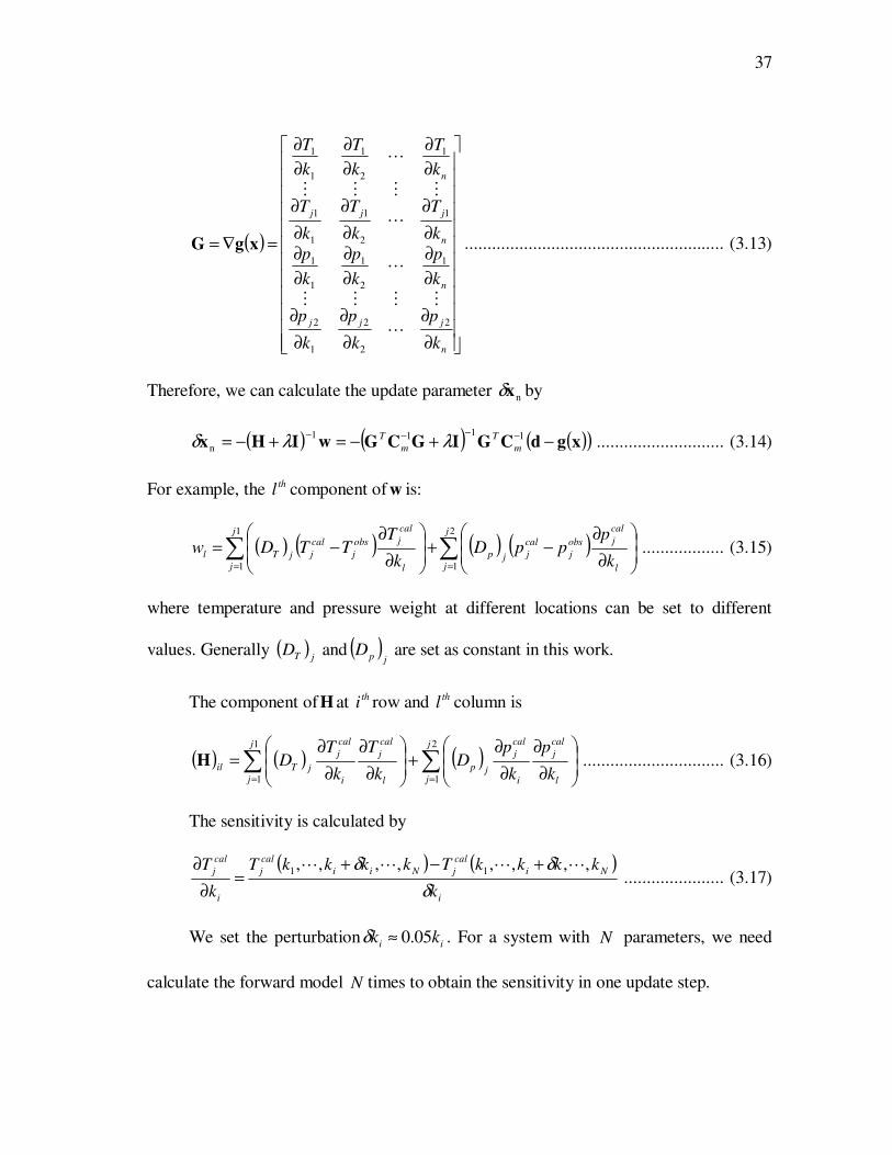
37

( )

∂

∂

∂

∂

∂

∂

∂

∂

∂

∂

∂

∂∂

∂

∂

∂

∂

∂

∂

∂

∂

∂

∂

∂

=∇=

n

jjj

n

n

jjj

n

k

p

k

p

k

p

k

p

k

p

k

p

k

T

k

T

k

T

k

T

k

T

k

T

2

2

2

1

2

1

2

1

1

1

1

2

1

1

1

1

2

1

1

1

L

MMMM

L

L

MMMM

L

xgG ......................................................... (3.13)

Therefore, we can calculate the update parameter nxδ by

( ) ( ) ( )( )xgdCGIGCGwIHx −+−=+−= −−−− 1111

n m

T

m

T λλδ ............................ (3.14)

For example, the thl component of w is:

( ) ( ) ( ) ( )∑∑==

∂

∂−+

∂

∂−=

2

1

1

1

j

j l

cal

jobs

j

cal

jjp

j

j l

cal

jobs

j

cal

jjTlk

pppD

k

TTTDw .................. (3.15)

where temperature and pressure weight at different locations can be set to different

values. Generally ( )jTD and ( )

jpD are set as constant in this work.

The component ofH at thi row and thl column is

( ) ( ) ( )∑∑==

∂

∂

∂

∂+

∂

∂

∂

∂=

2

1

1

1

j

j l

cal

j

i

cal

j

jp

j

j l

cal

j

i

cal

j

jTilk

p

k

pD

k

T

k

TDH ............................... (3.16)

The sensitivity is calculated by

( ) ( )

i

Ni

cal

jNii

cal

j

i

cal

j

k

kkkkTkkkkT

k

T

δ

δδ ,,,,,,,, 11 LLLL +−+=

∂

∂...................... (3.17)

We set the perturbation ii kk 05.0≈δ . For a system with N parameters, we need

calculate the forward model N times to obtain the sensitivity in one update step.

38

In Eq. 3.14, the optimum value of the damping factorλ will affect the update

parameter. We can change λ to λ10 and 10/λ respectively, and then get three update

parameters: ( )λδx , ( )λδ 10x , and ( )10/λδx . The next step is to calculate the objective

function based on these three update parameters, and choose the one with minimum

objective function as the best update parameter. The initial λ can be estimated by the

average eigenvalue of the Hessian matrix.

Therefore, starting from an initial guess 0x , we can use Eq. 3.14 to calculate the

update parameter xδ iteratively. The iteration will stop when the objective function

converges by using the following criteria:

( ) ( ) 11nn ε<− +xfxf ....................................................................................... (3.18)

or

( ) ( )( ) 2

n

1nn ε<− +

xf

xfxf....................................................................................... (3.19)

where 1ε and 2ε are relative small residuals. Eq. 3.19 are more useful because 2ε is

dimensionless, and the effect of weights on the objective function is almost cancelled by

division. Generally, 2ε can be 0.001~0.01.

3.2 MARKOV CHAIN MONTE CARLO METHOD

Markov chain Monte Carlo (MCMC) method is generally used in sampling (Ma et al.,

2008; Oliver et al., 1997). In this work, we use the traditional Metropolis-Hasting

MCMC Algorithm to minimize the objective function. The procedure of this method is

following these steps:

39

1. Guess an initial reservoir permeability distribution 0k .

2. At state n , for a given initial permeability distribution nk , run the forward model,

and get calculated temperature and pressure data.

3. Calculate the objective function ( )nkf .

4. Generate 1+nk from a proposal distribution )|( 1 nnd kkq + . In this work, we use

uniform distribution to generate the new permeability.

5. Run forward model, get new pressure and temperature data, and calculate the

objective function ( )1+nkf .

6. Use Metropolis-Hastings algorithm to judge the acceptance of 1+nk .

7. If the new permeability is accepted, store the new permeability as the next state

and go to step 2, otherwise, go to step 4.

The Metropolis-Hastings (M-H) algorithm is applied in step 6 to decide the

acceptance of any new generated permeability, i.e., the proposed permeability

distribution, 1+nk , is accepted according to the probability:

( ) ( ) ( )( )( ) ( )( )

=

+

+++

nnnd

nnndnnprob

kEXPkkq

kEXPkkqkk

f-

f-

1

111

|

|,1min,ρ ....................................... (3.20)

After a series of sampling (known as burn-in), we collect samples 0k , 1k , 2k , …, nk ,

1+nk ,…, which are possible solutions to the inverse problem.

The sampler method in step 4 will significantly affect the acceptance of the

MCMC method. The independent sampler is a proposal that generates sampler from a

uniform distribution without the bound to the current condition. This makes the

40

inversion process very slow. Therefore, we try to find some other sampler to increase the

efficiency.

The random walk sampler is generated by perturbing the current model (Ma et

al., 2008). Generally, the random walk sampler has a higher acceptance rate. The

random walk sampler first generates a model from uniform distribution, and then uses

the current model to constrain the new model:

ε+= nkk .................................................................................................... (3.21)

The small perturbation ε is set about nk1.0± . If a new model generated form

the uniform distribution does not satisfy Eq. 3.21, we reject it and generate a new model

until it agrees with the constraint.

Additionally, the generated permeability distribution may be also conditioned

by temperature trend or temperature derivative, which can avoid some obvious

impossible samples. In the MCMC method, the new model is accepted by using the M-H

algorithm in Eq. 3.20. The value of the objective function will influence on the

acceptance. Therefore, the value of temperature and pressure weights will affect the

result. In this work, the temperature weight, TD , can be set to 200~2000, and the

pressure weight can be estimated by Eq. 3.3.

3.3 FEASIBILITY OF INVERSION OF TEMPERATURE, PRESSURE AND

FLOW

A simple synthetic case is used to exam the validation of the inversion program. Fig. 3.1

shows the geometry of this case. Assume the reservoir is separated to two zones, an oil

41

zone and a water zone. The horizontal well is located at the center of the reservoir, and it

is fully penetrated. Table 3.1 is the reservoir input. The reservoir boundaries at y

direction are set as constant pressure boundary. Other reservoir boundaries are set as no

flow boundary. The initial temperature in reservoir is geothermal distributed

temperature. Table 3.2 lists the fluid and rock properties.

Fig. 3.1 Reservoir geometry information for validation case

Table 3.1 Reservoir and Well Parameters in Program Validation

Reservoir Wellbore

Drainage area, ft×ft 3000×2000 Depth of the wellbore, ft 6045

Thickness, ft 90 Length of wellbore, ft 3000

Depth of top, ft 6000 Liquid production rate,

bbl/d

10000

Porosity 0.2 Wellbore diameter, ft 0.75

Permeability, kh (kh=10kv), md

Oil zone

Water zone

100

25

Wellbore location in y-

direction, ft

1000

Initial temperature at 6000 ft,

0F

180 Casing diameter, in. 6

Geothermal gradient, 0F/ft 0.01 Casing roughness 0.0005

42

Table 3.2 Fluid and Rock Properties

Oil Water Rock

Density (lb/ft3) 50 63 165

Viscosity (cp) 1 0.48

Heat capacity (Btu/lb-0F) 0.516 1.002 0.22

Thermal expansion

coefficient ×104 (1/0F) 6.79 3.11

Total thermal conductivity,

TtK (Btu/hr-ft-0F) 2.0

Using this input data, the temperature, pressure, and flow rates can be

calculated from the forward model. Fig. 3.2 shows the pressure, Fig. 3.3 gives the

temperature, and Fig. 3.4 shows the oil and water flow rate distribution. They are

referred as observed data, which are marked by triangles in these Figures.

Once the observed data are generated from the forward calculation, the

inversion program is applied. Here it adopts MCMC method with random walk sampler.

Assume that we already know the locations of oil zone and water zone, the unknown

parameters are the permeabilities in the oil zone and the water zone.

Starting from a homogenous initial guess, the inversion program uses 50 md for

the entire reservoir permeability. The calculated pressure and temperature at initial

condition are different from the observed data. The inverted pressure and temperature

which satisfy convergence criteria are marked as lines in Fig. 3.2 and Fig. 3.3. The

inverted permeability at matching condition is shown in Fig. 3.5. The corresponding

43

flow rates of oil and water are close to the observed data, as shown in Fig. 3.4. The

results indicate that the inversion program can be used for further study.

3600

3640

3680

3720

3760

3800

0 500 1000 1500 2000 2500 3000

Well distance from heel, ft

Pre

ssu

re, p

si

Observed

Inverted

Initial Test

Fig. 3.2 Observed and inverted pressure data at 60 days

180.5

180.55

180.6

180.65

180.7

0 500 1000 1500 2000 2500 3000

Well distance from heel, ft

Tem

pera

ture

, 0F

Observed

Inverted

Initial test

Fig. 3.3 Observed and inverted temperature data at 60 days

44

0

2000

4000

6000

8000

10000

0 500 1000 1500 2000 2500 3000

Well distance from heel, ft

Flo

w r

ate

in

well, b

bl/d

TrueInvertedOil

Water

Fig. 3.4 Observed and inverted flow rates of validation case

0

50

100

150

200

0 500 1000 1500 2000 2500 3000

Well distance from heel, ft

Perm

eab

ilit

y, m

d

True

Inverted

Initial

Fig. 3.5 Inverted permeability distribution of validation case

45

4 CHAPTER IV

RESULTS OF TEMPERATURE INTERPRETATION MODEL

In this chapter, examples will be used to show how the new model can be applied to the

problems at field conditions. We will show the result of forward model first, and then the

inversion process. The examples include two cases of water breakthrough diagnosis. The

first example is a bottom water driving case, and the second one is a water injection

case.

4.1 EXAMPLE 1: BOTTOM WATER DRIVING

The first synthetic example is bottom-aquifer drive case. The example reveals the

relation between temperature and flow rate, therefore builds the foundation of the

inversion process.

4.1.1 Forward Model Results

One of the biggest problems of bottom-aquifer drive formation is water coning. The

problem becomes more severe when reservoir permeability heterogeneity is involved.

Fig. 4.1 shows the schematic of the example. The physical model is a rectangular shaped

oil reservoir. There is an infinite water support from the bottom aquifer. The horizontal

well is located 35 ft from the top boundary of 100-ft payzone (Fig. 4.2b). Fig. 4.2 shows

the permeability distribution and relative permeability curve use in this water-oil two-

phase flow example. The horizontal permeability is 10 times of the vertical permeability.

46

The reservoir permeability varies along the wellbore. It has a lower permeability zone

(10 md) from 600 to 1200 ft in the x-direction, and a higher permeability zone (500 md)

from 1800 to 2100 ft. The rest of the reservoir has a permeability of 50 md.

a. 3D geometry b. front view geometry

Fig. 4.1 Reservoir geometry information of bottom water driving case

P1

X

Y

0 500 1000 1500 2000 2500 3000 3500

0

500

1000

1500

2000

0.0000 43.2377 120.1265 256.8563 500.0000PERMX

0

0.2

0.4

0.6

0.8

1

0 0.2 0.4 0.6 0.8 1

Sw

Rela

tive p

erm

eab

ilit

y

krw

kro

a. grid and permeability distribution b. relative permeability

Fig. 4.2 Reservoir permeability distribution and relative permeability curve

47

Table 4.1 lists the formation and wellbore information, and fluid properties at

reference temperature (180 0F) and pressure (4000 psi) is listed in Table 3.2. The initial

temperature at the top surface of the formation is 180 0F.

Table 4.1 Input for Reservoir and Wellbore of Water Driving Example

Reservoir Wellbore

Drainage area, ft×ft 3600×2000 Depth of the wellbore, ft 6035

Thickness, ft 100 Length of wellbore, ft 3000

Depth of top, ft 6000 Liquid production rate, bbl/d 10000

Water oil contact, ft 6100 Wellbore diameter, ft 0.75

Porosity 0.2 Casing diameter, in. 6

Permeability, md 10,50,500 Casing roughness 0.001

Initial temperature at 6000

ft, 0F

180 Wellbore location in y-

direction, ft

1000

Geothermal gradient, 0F/ft 0.01

For the given condition, we use the forward model to predict the oil and water

flow rates and the temperature and pressure distributions. Fig. 4.3 through Fig. 4.6 show

the calculated results at the wellbore. Fig. 4.3 is the oil inflow rate distribution, Fig. 4.4

is the water inflow rate distribution, Fig. 4.5 is the wellbore temperature, and Fig. 4.6 is

the wellbore pressure. Because of the heterogeneity in the permeability field, we observe

a non-uniformed temperature along the wellbore, as seen in Fig. 4.5. As production time

increase, the anomalous feature on the temperature curve becomes more pronounced.

Naturally, when the permeability is high, more fluid with higher temperature enters the

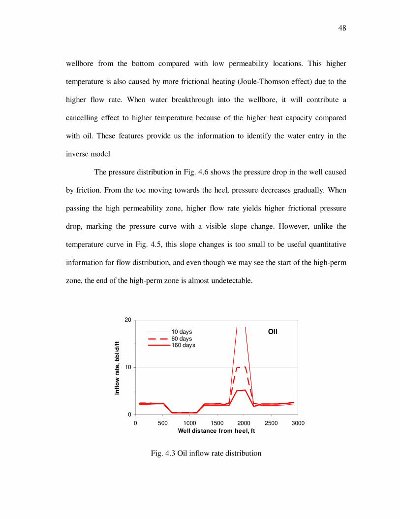
48

wellbore from the bottom compared with low permeability locations. This higher

temperature is also caused by more frictional heating (Joule-Thomson effect) due to the

higher flow rate. When water breakthrough into the wellbore, it will contribute a

cancelling effect to higher temperature because of the higher heat capacity compared

with oil. These features provide us the information to identify the water entry in the

inverse model.

The pressure distribution in Fig. 4.6 shows the pressure drop in the well caused

by friction. From the toe moving towards the heel, pressure decreases gradually. When

passing the high permeability zone, higher flow rate yields higher frictional pressure

drop, marking the pressure curve with a visible slope change. However, unlike the

temperature curve in Fig. 4.5, this slope changes is too small to be useful quantitative

information for flow distribution, and even though we may see the start of the high-perm

zone, the end of the high-perm zone is almost undetectable.

0

10

20

0 500 1000 1500 2000 2500 3000

Well distance from heel, ft

Infl

ow

ra

te,

bb

l/d

/ft

10 days60 days160 days

Oil

Fig. 4.3 Oil inflow rate distribution

49

0

10

20

0 500 1000 1500 2000 2500 3000

Well distance from heel, ft

Infl

ow

rate

, b

bl/d

/ft

160 days

60 days

Water

Fig. 4.4 Water inflow rate distribution

180.3

180.5

180.7

180.9

181.1

0 500 1000 1500 2000 2500 3000Well distance from heel, ft

Tem

pera

ture

, 0F

1 day

10 days

60 days

160 days

low perm

high perm

Fig. 4.5 Temperature distribution in wellbore

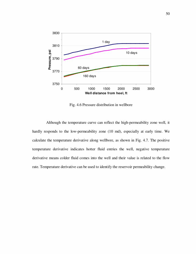
50

3750

3770

3790

3810

3830

0 500 1000 1500 2000 2500 3000

Well distance from heel, ft

Pre

ssu

re, p

si

1 day

10 days

60 days

160 days

Fig. 4.6 Pressure distribution in wellbore

Although the temperature curve can reflect the high-permeability zone well, it

hardly responds to the low-permeability zone (10 md), especially at early time. We

calculate the temperature derivative along wellbore, as shown in Fig. 4.7. The positive

temperature derivative indicates hotter fluid entries the well, negative temperature

derivative means colder fluid comes into the well and their value is related to the flow

rate. Temperature derivative can be used to identify the reservoir permeability change.

51

-0.1

0

0.1

0.2

0.3

0.4

0.5

0 500 1000 1500 2000 2500 3000

Well distance from heel, ft

dT

/(seg

men

t),

0F

160 days

100 days

Fig. 4.7 Temperature derivative in wellbore

One advantage of the new model compared with the previous model by

Yoshioka et al. (2007b) is that the reservoir temperature, pressure and flow are simulated

as a function of time. This transient flow condition provides additional information such

as derivatives and helps us to interpret flow profile from temperature and pressure data

more accurately. We examine the transient wellbore temperature at two locations, inside

the water zone (2025 ft) and outside the water zone (2625 ft) and the water cut as a

function of time (shown in Fig. 4.8, temperature as a function of time). The interesting

result is that small temperature drop occurs on the temperature curve when water breaks

in. The explanation is that the arriving water temperature at this time is lower than the oil

temperature because of the difference in heat capacity of these two fluids. Therefore,

when the water breaks through, the arriving temperature will decrease. This feature can

52

help us to locate water breakthrough location and time. Noticed that this temperature

drop is very small, it may require certain sensor resolution to identify the change.

180.2

180.6

181

0 50 100 150 200

Time, day

Tem

pera

ture

, 0F

0

0.4

0.8

Wate

r cu

t

x = 2625 ft

x = 2025 ft

water cut

small T drop

indicates

water entry

Fig. 4.8 Water cut history and transient temperature at two locations

The transient wellbore temperature distribution as a function of time is shown

in Fig. 4.9, and the transient arriving temperature distribution is shown in Fig. 4.10.

Temperature increases very fast at early time and becomes slower at later time. It is

because that Joule-Thomson effect domains the temperature change at earlier time. One

explanation is that pressure change is significant at early time; as well as the flow near

wellbore is mainly radial, so the temperature change caused by the Joule-Thomson effect

is fastest at early time. At late time, temperature change caused by Joule-Thomson effect

is slower, but the vertical flow will bring hot fluid from the bottom. The range where the

flow rate is higher will have more obvious temperature increase.

53

Additionally, the transient arriving temperature (Fig. 4.10) can reflect each

different permeability range much better than the wellbore temperature. This

temperature is the fluid temperature before mixing with fluids in wellbore, so it keeps

more original reservoir geology information.

Well Distance, ft

01000

20003000 Time, day

050

100150

Te

mp

er a

ture

,F180.4

180.6

180.8

181

181.2

Fig. 4.9 Transient wellbore temperature distribution

Well Distance, ft

0

1000

2000

Time, day050

100150

Te

mp

era

tur e

,F

180.4

180.6

180.8

181

181.2

Fig. 4.10 Transient arriving temperature distribution

54

4.1.2 Inversion Results

Based on the forward model, inversion methods can be applied to interpret downhole

measurements, temperature and pressure data, to flow conditions using the same

example in the previous section of forward model results. Fig. 4.11 is the top view of the

reservoir and wellbore geometry. The forward-model-calculated data presented in Fig.

4.5 will be referred as observed data (corresponding to the measured data in the field).

Suppose we have observed temperature and pressure data shown in Fig. 4.5 and Fig. 4.6

from DTS or production logging, and we choose the data at 160 days as the observed

data for interpretation. The objective is to interpret the flow profile as shown in Fig. 4.3

and Fig. 4.4 by the inverse model.

To start the process, we analyze the observed temperature data, as marked in

Fig. 4.12 as the triangles, where the temperature derivative is also plotted as the solid

line. Initially, we assign a uniform permeability of 65 md in the entire reservoir. With

this permeability field, we calculate flow rates, wellbore pressure, and temperature by

the forward model. With the initial guess, the calculated temperature is plotted against

the observed data in Fig. 4.12 as the dashed line. Comparing this calculated temperature

and the observed data, we know that the permeability from 2100 to 3000 ft should be

close to 65 md, and permeability from 1800 to 2100 ft should be higher than 65 md. The

calculated temperature with assumed permeability of 65 md is much lower than the

observed temperature, indicating less warm fluid entering the wellbore at this location.

The details also can be confirmed by the temperature derivative, which also detects a

55

slightly low permeability range from 600 to 1200 ft because the slope has smallest

absolute value.

Because the wellbore is not fully penetrated in the reservoir for this case,

temperature data along the horizontal wellbore is only measured from 0 to 3000 ft. For

the unknown permeability from 3000 to 3600 ft, we assume that it is the same as the

permeability at the range from 2100 to 3000 ft.

Based on this analysis of the observed temperature data and its derivative, we

separate the reservoir to five segments: from 0 to 600 ft is zone 1, 600 to 1200 ft as zone

2, 1200 to 1800 ft as zone 3, 1800 to 2100 ft as zone 4, and 2100 to 3600 ft as zone 5.

Each zone has a permeability value as the parameter for inversion. Now we can use

either Levenberg-Marquardt (L-M) method or MCMC method to minimize the objective

function by finding a satisfied permeability field.

P1

X

Y

0 500 1000 1500 2000 2500 3000 3500

0

500

1000

1500

2000

Fig. 4.11 Top view of reservoir and wellbore

56

180.2

180.4

180.6

180.8

181

181.2

0 500 1000 1500 2000 2500 3000

Well distance from heel, ft

Tem

pera

ture

, 0F

-0.2

0

0.2

0.4

0.6

0.8

dT

/seg

men

t,

0F

1 2 3 4 5

T

dT/segment

Fig. 4.12 Separate reservoir to sections by temperature data

L-M Method Inverted Results

We use two different permeability distributions as initial guess for the inversion process.

One is a homogenous initial guess, which we assign a uniform permeability of 100 md to

the entire reservoir, and another one is a 2-value initial guess, which are 200 md from

1800 to 2100 ft and 100 md for other ranges. Fig. 4.13 shows that the objective function

decreases vs. iteration number during the inversion process. The objective function at

these two initial conditions becomes converged (the objective function approaches a

constant) when the program iterates about 30 times. For the homogenous initial guess,

the calculated result does not perfectly fit the observed data. But for the 2-value initial,

the objective function is close to the zero, which means that calculated result fits the

observed data very well. Fig. 4.13 reveals that the inversion result of L-M method is

depending on the initial conditions.

57

0

500

1000

1500

2000

2500

0 5 10 15 20 25 30 35

Iteration number

Ob

jecti

ve f

un

cti

on

Homogenous Initial

2-Value Initial

Fig. 4.13 Objective function vs. iteration number at two initial conditions

Homogenous Initial Permeability Result

The inverted result with a uniform permeability of 100 md to the entire reservoir as

initial guess for the L-M method is showed in Fig. 4.14 and Fig. 4.15. Fig. 4.14 is the

forward-model-calculated temperature (inverted temperature) when the objective

function gets convergence. Fig. 4.15 is the inverted pressure. Compared with the

temperature calculated from the homogenous initial guess, the inverted temperature is

closer to the observed data. It follows the trend of the observed data, although there is a

certain error at the sections from 0 to 2000 ft.

However, compared with the initial guess, the inverted pressure does not

converge to the observed data even when the objective function converges. This

difference is the reason that objective function is still big.

58

180.2

180.4

180.6

180.8

181

181.2

0 500 1000 1500 2000 2500 3000

Well distance from heel, ft

Tem

pera

ture

, 0F

Observed

Inverted

Initial

Fig. 4.14 Matched temperature data from L-M method, homogenous initial

3720

3770

3820

3870

0 500 1000 1500 2000 2500 3000

Well distance from heel, ft

Pre

ssu

re, p

si

Observed

Inverted

Initial

Fig. 4.15 Matched pressure data from L-M method, homogenous initial

Once the inversion process stops, it means that the program finds a permeability

distribution which makes the objective function achieved a minimum, i.e., the forward-

59

model-calculated temperature and pressure at this permeability distribution match the

observed data. We plot the inverted flow rate profiles of oil and water at this condition in

Fig. 4.16, and the inverted permeability distribution is shown in Fig. 4.17. The inverted

oil rate profile is acceptable, but the water rate profiles have a certain error, and the

water entry location is not correct. The inverted result requires improvement because the

objective function is still a significant number.

0

2000

4000

6000

8000

0 500 1000 1500 2000 2500 3000

Well distance from heel, ft

Flo

w r

ate

in

we

ll, b

bl/d

TrueInvertedOil

Water

Inverted water rate unsatisfied

Fig. 4.16 Inverted oil and water flow rate profiles from L-M method, homogenous initial

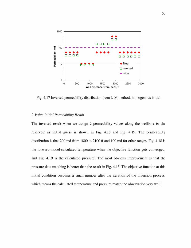
60

1

10

100

1000

0 500 1000 1500 2000 2500 3000

Well distance from heel, ft

Perm

eab

ilit

y, m

d

True

Inverted

Initial

Fig. 4.17 Inverted permeability distribution from L-M method, homogenous initial

2-Value Initial Permeability Result

The inverted result when we assign 2 permeability values along the wellbore to the

reservoir as initial guess is shown in Fig. 4.18 and Fig. 4.19. The permeability

distribution is that 200 md from 1800 to 2100 ft and 100 md for other ranges. Fig. 4.18 is

the forward-model-calculated temperature when the objective function gets converged,

and Fig. 4.19 is the calculated pressure. The most obvious improvement is that the

pressure data matching is better than the result in Fig. 4.15. The objective function at this

initial condition becomes a small number after the iteration of the inversion process,

which means the calculated temperature and pressure match the observation very well.

61

180.2

180.4

180.6

180.8

181

181.2

0 500 1000 1500 2000 2500 3000

Well distance from heel, ft

Tem

pera

ture

, 0F

Observed

Inverted

Initial

Fig. 4.18 Matched temperature data from L-M method, 2-vlue initial

3720

3770

3820

3870

0 500 1000 1500 2000 2500 3000

Well distance from heel, ft

Pre

ss

ure

, p

si

Observed

Inverted

Initial

Fig. 4.19 Matched pressure data from L-M method, 2-vlue initial

At this condition that temperature and pressure matched the observation, the

inverted oil and water flow rate profiles are showed in Fig. 4.20. Compared with the

62

result in Fig. 4.16, this result is improved, and the water entry location is found

correctly. Fig. 4.21 shows the inverted permeability distribution which is very close to

the true data at zone 1 (0 to 500 ft), zone 4 (1800 to 2100 ft), and zone 5 (2100 to 3600

ft). Because these sections dominate the reservoir flowing, the error at other sections

becomes small and it is acceptable.

0

2000

4000

6000

8000

0 500 1000 1500 2000 2500 3000

Well distance from heel, ft

Flo

w r

ate

in

we

ll, b

bl/d

TrueInvertedOil

Water

Fig. 4.20 Inverted oil and water flow rate profiles from L-M method, 2-vlue initial

63

1

10

100

1000

0 500 1000 1500 2000 2500 3000

Well distance from heel, ft

Pe

rmeab

ilit

y, m

d

True

Inverted

Initial

Fig. 4.21 Inverted permeability distribution from L-M method, 2-vlue initial

MCMC Inverted Results

In this section, we use MCMC to minimize the objective function. According to the

previous analysis of the temperature data, the reservoir is separated to five segments:

zone 1 to zone 5. The permeability in each zone is the unknown parameter which needs

to be determined from inversion.

For the MCMC method, we will randomly search the permeability in the global

space. However, because we already diagnose that the range from 1800 to 2100 ft has

obviously higher permeability, the searching range can be conditioned. In this work, we

search the permeability from 100 to 1000 md for the high permeability range (1800 to

2100 ft) and 10 to 100 md for all other zones. Because the low permeability section (600

to 1200 ft) is detected, the program will reject any permeability generated here with

higher value, which increases the efficiency of convergence.

64

The convergence of objective function using MCMC method is shown in Fig.

4.22. We only plot the accepted number during the inversion problem. The independent

sampler, which independently generates 1+nk , has very low acceptance, and it is time

consuming. The random walk sampler, which is constrained by current model in Eq.

3.21, has higher acceptance, and it gets satisfied result faster.

0

400

800

1200

1600

2000

0 3 6 9 12 15Accepted number

Ob

jecti

ve f

un

cti

on

0 10 20 30 40 50

Independent sampler, 400 runs

Random w alk sampler, 180 runs

Fig. 4.22 Objective function converges

At the convergence condition, Fig. 4.23 and Fig. 4.24 show that the inverted

temperature and pressure match well with the observed data, implying that flow

conditions are close to the true conditions.

65

180.2

180.4

180.6

180.8

181

181.2

0 500 1000 1500 2000 2500 3000

Well distance from heel, ft

Tem

pera

ture

, 0F

Observed

Inverted

Initial test

Fig. 4.23 Matched temperature data from MCMC method

3750

3770

3790

3810

3830

0 500 1000 1500 2000 2500 3000

Well distance from heel, ft

Pre

ssu

re, p

si

Observed

Inverted

Initial test

Fig. 4.24 Matched pressure data from MCMC method

As the result, we plot inverted flow profiles in Fig. 4.25 and inverted

permeability distribution in Fig. 4.26. Inverted flow profiles are acceptable. It identifies

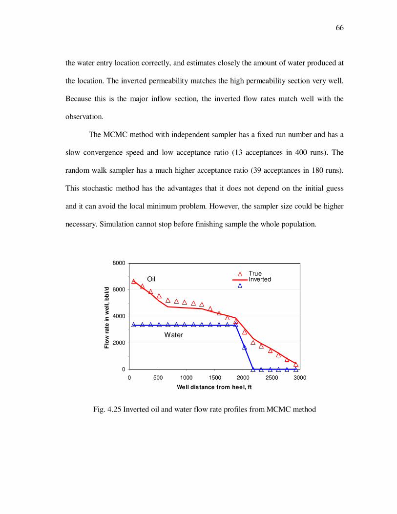
66

the water entry location correctly, and estimates closely the amount of water produced at

the location. The inverted permeability matches the high permeability section very well.

Because this is the major inflow section, the inverted flow rates match well with the

observation.

The MCMC method with independent sampler has a fixed run number and has a

slow convergence speed and low acceptance ratio (13 acceptances in 400 runs). The

random walk sampler has a much higher acceptance ratio (39 acceptances in 180 runs).

This stochastic method has the advantages that it does not depend on the initial guess

and it can avoid the local minimum problem. However, the sampler size could be higher

necessary. Simulation cannot stop before finishing sample the whole population.

0

2000

4000

6000

8000

0 500 1000 1500 2000 2500 3000

Well distance from heel, ft

Flo

w r

ate

in

well, b

bl/d

TrueInvertedOil

Water

Fig. 4.25 Inverted oil and water flow rate profiles from MCMC method

67

1

10

100

1000

0 500 1000 1500 2000 2500 3000

Well distance from heel, ft

Pe

rmeab

ilit

y, m

d

True

Inverted

Initial

Fig. 4.26 Inverted permeability distribution from MCMC method

The gradient based method, the Levenberg-Marquart (L-M) method, depends

on the initial condition and might be stuck in the local minimum. According to our test

on this synthetic example, with a good initial guess, the L-M method has a quicker

converging speed than MCMC method. But at some initial situations, it cannot obtain a

satisfied result.

Either L-M method or MCMC method can be used. In this study, MCMC

method is used for the following synthetic cases and field applications.

4.2 EXAMPLE 2: WATER INJECTION

Temperature data can also be used to identify water entry in water flooding cases. This

example is applied to a 2D permeability field to illustrate that the inversion procedure

can be used in the complex permeability situations.

68

4.2.1 Forward Model Results

For a water-injection system, Fig. 4.27 shows the reservoir geometry and the well

locations. The reservoir has a horizontal injection well and a horizontal producing well.

They are parallel and locate at the middle of the pay zone in vertical direction.

Table 4.2 gives the reservoir and production well information. The injection

well has a constant bottomhole pressure, 4000 psi, locates at 1995 ft in the y direction,

and the pressure drop in injection well is ignored. The injected water has a constant

temperature of 100 0F. Temperature effect on pressure and saturation solution is

neglected. The 2D permeability distribution for this case is shown in Fig. 4.28.

Fig. 4.27 Reservoir geometry and well locations

69

X

Y

0 500 1000 1500 2000 2500 3000

0

500

1000

1500

2000

0 90 180 270 360PERMX

Fig. 4.28 2D permeability distribution

Table 4.2 Input for Reservoir and Wellbore of Water Injection Example

Reservoir Production Wellbore

Drainage area, ft×ft 3000×2000 Depth of the wellbore, ft 6025

Thickness, ft 50 Length of wellbore, ft 3000

Depth of top, ft 6000 Liquid production rate, bbl/d 6000

Porosity 0.2 Wellbore diameter, ft 0.75

Initial temperature at 6000

ft, 0F

180 Casing roughness 0.001

Geothermal gradient, 0F/ft 0.01 Casing diameter, in. 4.5

The oil flow rate profiles at 300, 600 and 900 days are shown in Fig. 4.29, and

the water flow rate profiles are shown in Fig. 4.30. The 2D heterogeneous permeability

causes a non-linear flow rate distribution in the wellbore.

70

0

2000

4000

6000

0 500 1000 1500 2000 2500 3000

Well distance from heel, ft

Flo

w r

ate

, b

bl/d

300 days600 days

900 days

Fig. 4.29 Oil flow rate profiles in tubing

0

2000

4000

6000

0 500 1000 1500 2000 2500 3000

Well distance from heel, ft

Flo

w r

ate

, b

bl/d

600 days

900 days

Fig. 4.30 Water flow rate profiles in tubing

The wellbore temperature distribution is shown in Fig. 4.31, and the wellbore

pressure distribution is shown in Fig. 4.32. The temperature curves still have the increase

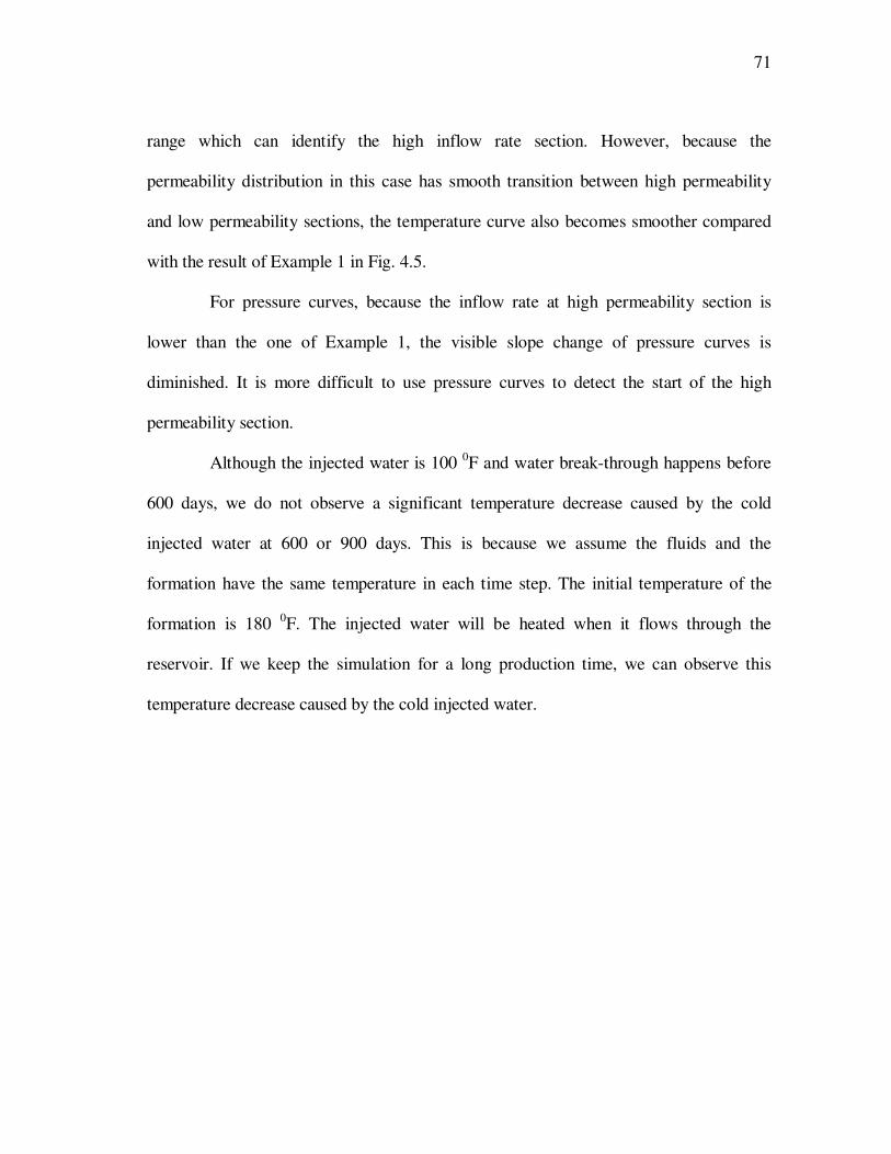
71

range which can identify the high inflow rate section. However, because the

permeability distribution in this case has smooth transition between high permeability

and low permeability sections, the temperature curve also becomes smoother compared

with the result of Example 1 in Fig. 4.5.

For pressure curves, because the inflow rate at high permeability section is

lower than the one of Example 1, the visible slope change of pressure curves is

diminished. It is more difficult to use pressure curves to detect the start of the high

permeability section.

Although the injected water is 100 0F and water break-through happens before

600 days, we do not observe a significant temperature decrease caused by the cold

injected water at 600 or 900 days. This is because we assume the fluids and the

formation have the same temperature in each time step. The initial temperature of the

formation is 180 0F. The injected water will be heated when it flows through the

reservoir. If we keep the simulation for a long production time, we can observe this

temperature decrease caused by the cold injected water.

72

180.4

180.5

180.6

180.7

180.8

180.9

0 500 1000 1500 2000 2500 3000

Well distance from heel, ft

Tem

pera

ture

, 0F

900 days

600 days

300 days

Fig. 4.31 Wellbore temperature distribution

3320

3340

3360

3380

0 500 1000 1500 2000 2500 3000

Well distance from heel, ft

Pre

ssu

re, p

si

900 days

600 days

300 days

Fig. 4.32 Wellbore pressure distribution

73

4.2.2 Inversion Results

The inversion procedure is applied to this example. Suppose that only temperature is

measured, as shown in Fig. 4.31. To start with, the reservoir is subdivided to several

sections according to the temperature trend or temperature derivative. Fig. 4.33 shows

reservoir sections inferred based on the temperature data. In each section, the

permeability is assigned a constant value. The permeabilities are considered unknown

variables that need to be determined from the inversion process. Because the measured

temperature is only along the horizontal well (x direction), the estimated reservoir

permeability distribution is aligned along the well as shown in Fig. 4.33.

180.4

180.5

180.6

180.7

180.8

180.9

0 500 1000 1500 2000 2500 3000

Well distance from heel, ft

Tem

pera

ture

, 0F

1 2 3 4 5

900 days

300 days

600 days

Fig. 4.33 Separate reservoir to sections by temperature data

First, the horizontal well temperature is calculated from the forward model by

adjusting the permeability value in each section, until the calculated temperature match

74

the observed data, as in Fig. 4.34. The inverted permeability at this temperature

matching condition is shown in Fig. 4.35, which is the contour of the true permeability

distribution. Although the temperature does not match perfectly, the simulated results

follow the trend of the observed data. The contour comparison in Fig. 4.35 indicates that

the temperature inverted permeability agrees with the true permeability qualitatively.

180.4

180.5

180.6

180.7

180.8

180.9

0 500 1000 1500 2000 2500 3000Well Distance from heel, ft

Tem

pe

ratu

re,

0F

ObservedCalculated 900 days

300 days

600 days

Fig. 4.34 Matched temperature data of water injection example

X

Y

0 500 1000 1500 2000 2500 3000

0

500

1000

1500

2000

0 90 180 270 360

PERMX

X

Y

0 500 1000 1500 2000 2500 3000

0

500

1000

1500

2000

0 90 180 270 360PERMX

Fig. 4.35 Temperature inverted perm vs. true perm, contour

75

Based on the temperature inverted permeability distribution, we also obtain

flow rate profiles for oil and water along the horizontal well at time 900 days in Fig.

4.36. The interpreted result of flow rate profiles is acceptable. The water entry location is

detected correctly, and the water and oil flow rate distributions are close to the reference

case.

0

2000

4000

6000

0 500 1000 1500 2000 2500 3000

Well Distance from heel, ft

Flo

w r

ate

in

well, b

bl/d

TrueInverted

Water

Oil

Fig. 4.36 Inverted water and oil flow rate profiles of water injection example

The arithmetic, geometric and harmonic means of inverted regions of the true

permeability distribution is calculated, and compared with the temperature-inverted

permeability, as shown in Fig. 4.37. The results indicate that the 1D temperature inverted

permeability, indeed, captures the basic characteristics of the true permeability field,

such as the low and the high permeability ranges.

The water-cut history calculated from the temperature inverted permeability

distribution is shown in Fig. 4.38. The simulated water-cut history follows the trend of

76

the observed data, but still shows significant mismatch. We can also see that the inverted

temperature at the high permeability section increases faster than the observed data.

Some of these discrepancies arise from the fact that the inverted permeability is only 1D,

which is an approximation of a 2D true permeability. An improved work including

production history information will be presented in Chapter V.

0

100

200

300

400

0 500 1000 1500 2000 2500 3000

Distance from heel, ft

Perm

eab

ilit

y, m

d

T inverted

arithmetic mean

geometric mean

harmonic mean

Fig. 4.37 Temperature inverted perm value vs. true perm average at y direction

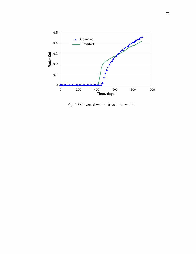
77

0

0.1

0.2

0.3

0.4

0.5

0 200 400 600 800 1000

Time, days

Wate

r C

ut

Observed

T Inverted

Fig. 4.38 Inverted water cut vs. observation

78

5 CHAPTER V

APPLICATIONS OF DOWNHOLE TEMPERATURE AND PRESSURE

MEASUREMENT

Three applications are presented in this chapter. Locating water or gas entry, optimizing

production in ICV equipped wells, and increasing resolution of reservoir characterization

by temperature information. The first application, locating gas or water entry in oil

producing wells, is a detailed expansion of the synthetic examples showed in Chapter

IV, here we apply the new method to some field cases.

In the second application, a procedure is provided to use temperature feedback to

control Inflow Control Valve (ICV) in horizontal well. After a series operation, the fluid

inflow rate along horizontal well is regulated by ICVs based on temperature feedback.

At this inflow rate condition, performance of horizontal well will be optimized.

The last application uses temperature measurement to assist reservoir

characterization and optimization. The temperature inversion only provided a coarse-

scale permeability distribution. Based on this temperature inverted permeability, and

coupling with a history matching method, the coarse permeability field is downscaled to

a fine permeability field, which includes both temperature and production history

information.

79

5.1 LOCATING GAS OR WATER ENTRY IN PRODUCING WELLS

5.1.1 Gas Entry in Oil Well

Gas entry in oil producing wells sometimes is detrimental. Problems mainly caused by

higher mobility of gas compared with oil. This can result choking back oil rate, tubing

limited production or surface facility limited production. This example is an oil/gas two

phase reservoir on the North Slope of Alaska. It is based on the published data by Brady

et al. (1998).

The reservoir has a strong gas cap. A horizontal well is placed 80 ft below the

gas-oil contact. It is assume the formation thickness is 100 ft, width is 1400 ft, and the

horizontal well is at the center of the width direction. The horizontal well was drilled

with 8.5” bit and completed with a 5.5” cement liner. And the casing ID is 4”. The

horizontal section is from 400 to 1900 ft of measured depth, which is also the producing

zone. The well was producing 2250 STB/d with a GOR of 2700 scf/STB when the

production logging was operated. The oil formation volume factor is about 1.2 bbl/STB,

and the gas formation volume factor is about 0.00848 rcf/SCF, which are estimated from

the origin paper.

The original paper does not provide clear pressure data. We assume the well was

operated at a constant pressure, 1800 psi (pwf), at the heel of the horizontal well. This

information is estimated from other examples in North Slope of Alaska (Frankenburg et

al., 2000). We set a 35 ft gas cap above the gas-oil contact, which has a constant pressure

of 2800 psi at the top boundary.

80

The fluid properties are estimated from the information about fluid at Prudhoe

Bay (Jerauld, 1997). Gas-oil relative permeability is also based on this source (Jerauld,

1997; Johnson et al., 1959). Table 5.1 lists some basic information we used in the

inversion process for the reservoir and wellbore system. The gas density will change

significantly when the pressure change is big, and they are calculated by empirical

relations (Dranchuk and Abou-Kassem, 1975).

Table 5.1 Input for Reservoir and Wellbore of Gas Entry in Oil Well Example

Reservoir Wellbore

Drainage area, ft×ft 1600×1400 Well heel depth, ft 5615

Formation Thickness, ft 100 Horizontal well length, ft 1500

Gas-oil contact, ft 5535 Wellbore diameter, ft 0.708

Porosity 0.2

Top initial temperature, 0F 177.5

Wellbore location at

drainage width, ft 700

Geothermal gradient, 0F/ft 0.015 Pressure at heel, psi 1800

Average kh (kh=10kv), md 8 Cement liner, in. 5.5

Oil viscosity, cp 1.2 Casing ID, in. 4

Gas viscosity (3500 psi), cp 0.0265 Roughness 0.001

First, we analyze the temperature data and its derivative, as shown in Fig. 5.1.

The temperature has an obvious low trend near 750 ft, indicating that gas enters into the

wellbore at this location, because gas has significant Joule-Thomson cooling effect. To

make gas enter into the wellbore at temperature decrease range, the reservoir

permeability at this location is assumed higher than the rest of well sections.

81

According to the analysis above, we assumed the reservoir can be segmented to

six sections with different permeability: 400 to 650 ft (zone 1), 650 to 735 ft (zone 2),

735 to 755 ft (zone 3), 755 to 775 ft (zone 4), 775 to 850 ft (zone 5), and 850 to 2000 ft

(zone 6). Each zone has its own permeability value. The permeability in zone 3 (735 to

755 ft) is the highest. The grids used in zone 1 to 6 are 50-ft, 25-ft, 10-ft, 25-ft, 50-ft and

100-ft respectively.

144

154

164

174

184

400 600 800 1000 1200 1400 1600 1800 2000

Measured Depth, ft

Tem

pera

ture

, 0F

-10

-3

4

11

18

dT

/seg

men

t,

0F

T

dT/segement

1 632 4 5

Fig. 5.1 Analysis on measured temperature

The inversion model was used then to find a permeability distribution that creates

a flow distribution along the wellbore. When the temperature calculated from the

generated flow distribution matches the measured temperature, the inversion is

completed. Fig. 5.2 shows the inverted temperature results.

82

162

164

166

168

170

172

174

176

178

180

182

184

400 600 800 1000 1200 1400 1600 1800 2000

Measured Depth, ft

Tem

pera

ture

, 0F Observed

CalculatedInitial (uniform 8md)

Fig. 5.2 Calculated temperature matches the measured data

When the temperature matches, we consider that the corresponding downhole

flow distribution at this condition should be the true rate. Fig. 5.3 shows the inverted gas

flow rate compared with the spinner measurement from production logging, and includes

the oil-rate comparison between our interpretation result and Brady et al.’s result. Fig.

5.4 is the inverted permeability distribution at the temperature matching condition. The

gas entry location detected by the new model agrees with the spinner interpretation

result, however, the interpreted gas rate by the new model has a sharper decline in zone

3 (735 to 755 ft) compared with the spinner interpretation.

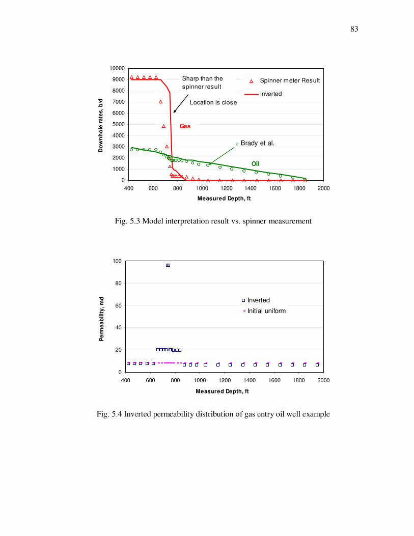
83

0

1000

2000

3000

4000

5000

6000

7000

8000

9000

10000

400 600 800 1000 1200 1400 1600 1800 2000

Measured Depth, ft

Do

wn

ho

le r

ate

s, b

/d

Spinner meter Result

Inverted

o Brady et al.

Sharp than the

spinner result

Location is close

Gas

Oil

Fig. 5.3 Model interpretation result vs. spinner measurement

0

20

40

60

80

100

400 600 800 1000 1200 1400 1600 1800 2000

Measured Depth, ft

Perm

eab

ilit

y, m

d Inverted

Initial uniform

Fig. 5.4 Inverted permeability distribution of gas entry oil well example

84

5.1.2 Water Entry in Oil Well

Water production is one of the biggest production problems today around the world.

Detecting water entry in a horizontal well is critical important in horizontal well

production. This example shows how to use the new method to interpret water entry

more precisely from temperature data.

The example is located in the Wandoo field, the North West Shelf of Australia

(Carnegie et al., 1998). Temperature and pressure data were measured by production

logging, which provided oil and water rates. Fig. 5.5 shows the field measured data.

Fig. 5.5 Field measured temperature, pressure and flow rates (Carnegie et al., 1998)

The formation is about 22 m thick and the oil zone is between a small overlying

gas cap and a strong aquifer. The gas-oil contact is at 577.3 m and the oil-water contact

Temperature

Pressure

Water rate Oil rate

85

is at 599.1 m. The gravity of the oil is 190 API with an in-situ viscosity of over 15 cp,

and the reservoir permeability ranges from 500 to 10,000 md. We use the range of

measured depth from 970 to 1930 m as the production zone in the model.

The horizontal well is located at about 585 m vertical depth. The length of the

well is about 1000 m, and the change of its true depth is less than 7 m. It is very close to

truly horizontal. The well was completed with pre-perforated liner and has a 9 5/8’’

casing cemented into 12.25’’ open hole. Because the formation width is not provided in

the paper, we assumed the reservoir width to be 667 m, and the horizontal well is located

at its center. At the surface, the observed surface flow rates were 3490 STB/d of oil, and

7265 STB/d of water at the time of production logging. The measured oil rate at the heel

of the horizontal well was about 5080 bbl/d. The difference of oil rate at surface and

downhole may be caused by the measured error of oil hold-up. In the inversion process,

for the horizontal well, we set a constant liquid flow rate of 10800 STB/d as the inner

boundary condition for pressure and saturation simulation.

Table 5.2 lists some basic input we used in this inversion process for the

reservoir and wellbore. Other thermal dynamic properties used here are the same as

Table 3.2.

86

Table 5.2 Input for Reservoir and Wellbore of Water Entry Oil Well Example

Reservoir Wellbore

Drainage area, m×m 960×667 Depth of the wellbore, m 585

Thickness, m 22 Horizontal well length, m 960

Top depth, m 577.3 Wellbore location at

drainage width, m

333.5

Water oil contact, m 599.1 Liquid production rate, bbl/d 10800

Porosity 0.2 Wellbore diameter, ft 1.021

Temperature at 575.8 m, 0F 124.7

Geothermal gradient, 0F/ft 0.01 Casing ID, in. 9.625

Oil viscosity, cp 15 Casing roughness 0.001

Water viscosity, cp 0.55

First, based on the observation of temperature data trend, we assumed the

reservoir can be segmented to six sections by permeability: zone 1 (970 to 1270 m), zone

2 (1270 to 1730 m), zone 3 (1730 to 1850 m), zone 4 (1850 to 1890 m), zone 5 (1890 to

1910 m), and zone 6 (1910 to 1930 m). The permeability in zone 5 should be the highest

because the highest measured temperature is located here. The permeability in zone 6 is

the second highest. Fig. 5.6 shows the measured temperature data with six segments.

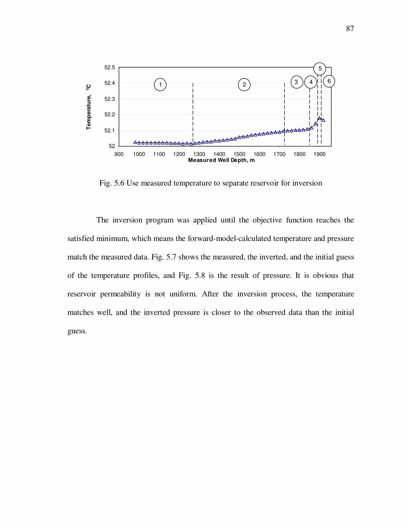
87

52

52.1

52.2

52.3

52.4

52.5

900 1000 1100 1200 1300 1400 1500 1600 1700 1800 1900Measured Well Depth, m

Tem

pera

ture

, 0C 1 2 3

5

4 6

Fig. 5.6 Use measured temperature to separate reservoir for inversion

The inversion program was applied until the objective function reaches the

satisfied minimum, which means the forward-model-calculated temperature and pressure

match the measured data. Fig. 5.7 shows the measured, the inverted, and the initial guess

of the temperature profiles, and Fig. 5.8 is the result of pressure. It is obvious that

reservoir permeability is not uniform. After the inversion process, the temperature

matches well, and the inverted pressure is closer to the observed data than the initial

guess.

88

51.8

51.9

52

52.1

52.2

52.3

900 1000 1100 1200 1300 1400 1500 1600 1700 1800 1900

Measured Well Depth, m

Tem

pera

ture

, 0C

Measured

Inverted

Initial (uniform)

Fig. 5.7 Match measured temperature data of water entry oil well example

760

780

800

820

900 1000 1100 1200 1300 1400 1500 1600 1700 1800 1900

Measured Well Depth, m

Pre

ssu

re, p

si

Measured

Inverted

Initial (uniform)

Fig. 5.8 Match measured pressure data of water entry oil well example

The inverted permeability at the temperature and pressure matching condition is

given in Fig. 5.9. The permeability at the toe of the horizontal wellbore is about 10~100

times higher than the permeability at other sections. According to Carnegie et al. (1998),

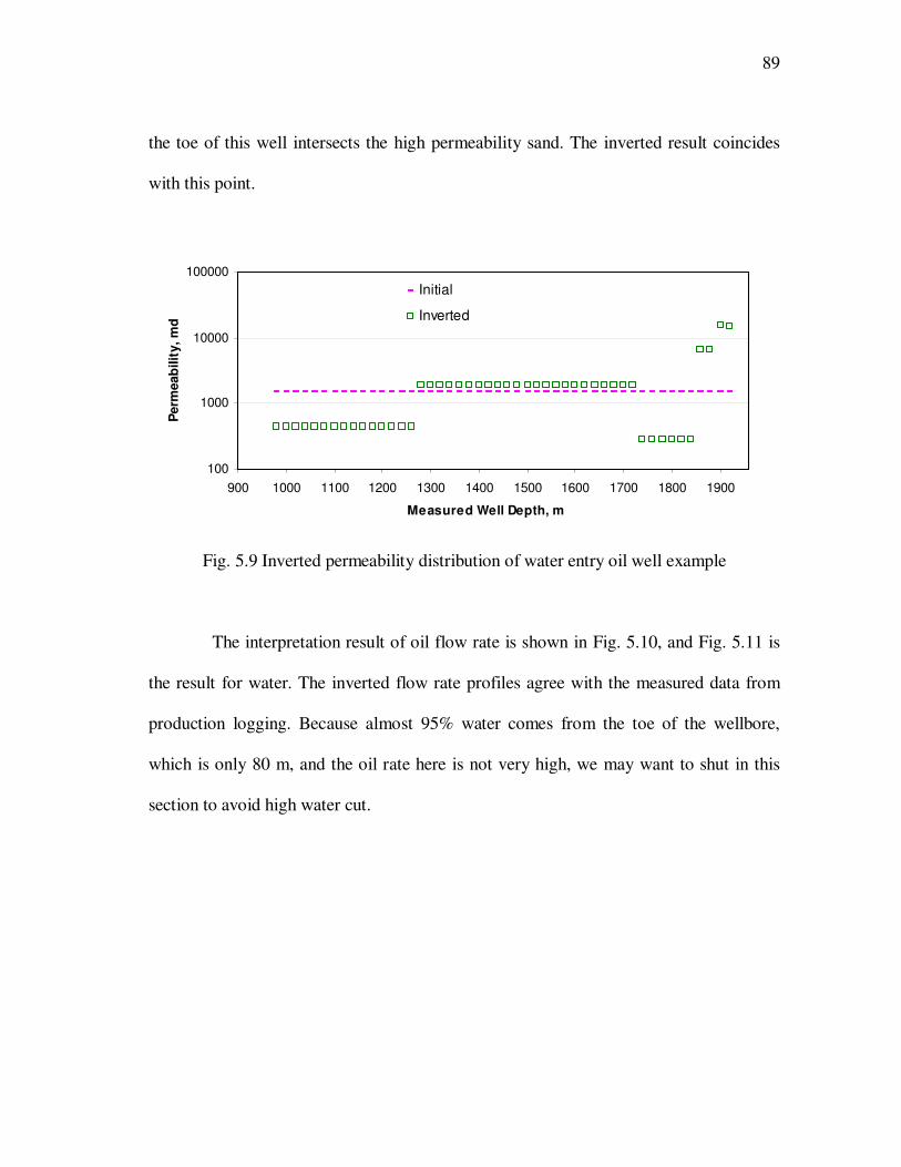
89

the toe of this well intersects the high permeability sand. The inverted result coincides

with this point.

100

1000

10000

100000

900 1000 1100 1200 1300 1400 1500 1600 1700 1800 1900

Measured Well Depth, m

Perm

eab

ilit

y, m

d

Initial

Inverted

Fig. 5.9 Inverted permeability distribution of water entry oil well example

The interpretation result of oil flow rate is shown in Fig. 5.10, and Fig. 5.11 is

the result for water. The inverted flow rate profiles agree with the measured data from

production logging. Because almost 95% water comes from the toe of the wellbore,

which is only 80 m, and the oil rate here is not very high, we may want to shut in this

section to avoid high water cut.

90

0

2000

4000

6000

8000

10000

900 1000 1100 1200 1300 1400 1500 1600 1700 1800 1900

Measured Well Depth, m

Flo

w r

ate

in

tu

bin

g, b

/dMeasured

Inverted

Initial

Fig. 5.10 Model interpretation compared with production logging measurement, oil

0

2000

4000

6000

8000

10000

900 1000 1100 1200 1300 1400 1500 1600 1700 1800 1900

Measured Well Depth, m

Flo

w r

ate

in

tu

bin

g, b

/d

Measured

Inverted

Initial

Fig. 5.11 Model interpretation compared with production logging measurement, water

5.1.3 Heavy Oil Well with Water Bottom

This example shows an oil producing well in the Zuata (Sincor) Field, Venezuela, which

is an extra heavy oil environment (Foucault et al., 2004). The formation is about 75 ft

thick. A high permeability zone of about 670 m with a permeability of 19 Darcy is the

91

target zone to produce heavy oil, and the measured depth of this zone is from 1244 to

1915 m. The reservoir has a bottom water-aquifer, and the well is set at 60 ft from the

bottom boundary of payzone. The reference pressure is 570 psi at the depth of the

horizontal well location. The horizontal well was completed with a 7” liner. Table 5.3

lists the reservoir and well information we used in the model as input. They are collected

from the original paper (Foucault et al.). Other thermal dynamic properties used here are

the same as Table 3.2. The temperature data was collected by downhole fiber optic

sensors.

We assumed a reservoir width of 667 m. The horizontal well is located at the

center of width. The temperature data was collected when the well was produced about 3

months, and it is shown in Fig. 5.12 as the curve with noise from 644 to 1800 m, which

includes vertical part of the well and no-producing zone. According to the temperature

data, we assumed the reservoir can be separated to three zones by permeability: zone 1

(1244 to 1750 m), zone 2 (1750 to 1800 m), and zone 3 (1800 to 1915 m). Each zone has

different permeability value and the permeability in 1750 to 1800 m is the highest. In the

forward model, the well produced 1000 stb/d at first 20 days, and then shut in for 60

days. After that, the well produced a constant liquid rate of 2400 stb/d.

92

Table 5.3 Input for Reservoir and Wellbore of Heavy Oil Well Example

Reservoir Wellbore

Reservoir Length, ft 2200 Diameter, ft 1

Reservoir Width, ft 2000 Length of wells, ft 2200

Formation Thickness, ft 75 Tubing diameter, in. 8

Temperature at formation

top, 0F

122.8 Tubing roughness 0.001

Geothermal gradient, 0F/ft 0.0157 Well distance to top, ft

Average kh (kh=10kv),

Darcy

19 0~1450 ft section 15

Oil viscosity, cp 2000 1450~2200 ft section 25

Water viscosity, cp 0.8

Because we do not have the numerical value of the observed temperature data

and the raw data contains noise, we use the forward model to match the raw data by

manually changing the permeabilities. Fig. 5.12 is the matched temperature data from

forward model calculation and the observed raw data. The matched temperature curve

has the same trend as the observed data, and its value is also close to the observed data.

The inverted permeability for the three sections is 19 Darcy, 46 Darcy, and 11 Darcy

respectively, showed in Fig. 5.13.

93

Fig. 5.12 Match measured DTS temperature data

0

25

50

544 744 944 1144 1344 1544 1744 1944

Measured depth, m

Perm

eab

ilit

y, D

arc

y

Inverted

Initial (Uniform)

Fig. 5.13 Inverted permeability distribution of heavy oil well example

In this case, we do not know downhole flow distribution, but the production

history at surface was provided. With the inverted permeability distribution, we also

successfully match the production history. Fig. 5.14 shows that the forward calculated

observed

94

result follows the trend of measurement, which indicates that the inverted permeability is

acceptable. Then we use this permeability to obtain oil and water flow profiles along the

wellbore, as shown in Fig. 5.15. Water comes into the well along the entire wellbore, but

it has a higher water inflow rate in the section of 1750 to 1800 m than other sections of

the well.

0

800

1600

2400

3200

4000

0 60 120 180 240 300 360

Time, days

Oil r

ate

, s

tb/d

0

0.2

0.4

0.6

0.8

1

Wate

r cu

t

Measured

Inverted

Water cut

Oil rate

Fig. 5.14 Inverted production history follows the trend of measurement

95

0

600

1200

1800

2400

544 744 944 1144 1344 1544 1744 1944

Measured depth, m

Flo

w r

ate

in

tu

bin

g, b

bl/d

water

oil

Fig. 5.15 Inverted flow rate profiles of oil and water

5.1.4 Water Entry in Gas Producing Well

This example diagnoses water entries in a gas well in Barnett shale. The reservoir has

extremely low matrix permeability from 0.00005 to 0.001 md, and its initial pressure is

about 3000 psi. The reservoir has no water aquifer. The horizontal well was

hydraulically fractured, and some water remained in the fractures. The horizontal well

was shut in for several years. It was re-opened after a long time shut in, and then

production logging was run to identify the gas and water entry locations in the well. Fig.

5.16 gives the measured temperature, and flow meter data. Pressure, well trajectory and

perforated locations are plotted in Fig. 5.17. At the surface, the gas flow rate of this well

is about 300 Mscf/d, and the water production rate is about 100 stb/d. The flow meter

measurement has suddenly decrease and increase at some location, and its trend is

complex. This is not a good response for interpretation. However, the measured

96

temperature data has obvious increasing and decreasing trends along the wellbore.

Generally, because of the pressure drop from reservoir to wellbore, the Joule-Thomson

effect will cause water temperature to increase, and gas temperature to decrease.

Therefore, according to the temperature trend in Fig. 5.16, we assume water comes into

the well at locations where temperature increases sharply, and gas enters into the well

mainly through locations where temperature decreases quickly.

Because the reservoir permeability is extremely low, the major entries of fluids

from reservoir to wellbore are from fractures. To use the model, we separate the

reservoir to a uniform size grid (50 ft) at horizontal well direction. It is hard to simulate

the exact fracture size by this model. Therefore, we assume high permeability for grids

where temperature has significant variation. These grids are assumed to include some

fractures, and the fracture effect is estimated by these equivalent high permeability

values. Because of the fracture, the difference of low and high permeability might be

very significant. So the porosity we used for low permeability sections is 0.04, and for

high permeability sections, it is 0.1. In addition, the well is perforated in almost each

grid.

From the measured temperature data, we can identify water entry locations.

Because the water comes from the remaining fluid after the hydraulic fracturing, we

assume the initial water saturation is close to 1.0 at these pre-identified locations in

reservoir. The reservoir top and bottom are no-flow condition, and the reservoir

boundary is assumed to be constant pressure.

97

163.5

164.0

164.5

165.0

165.5

4600 5100 5600 6100 6600 7100 7600Measured depth, ft

Tem

pera

ture

, 0F

-5

-3

-1

1

3

Flo

w m

ete

r, r

ps

Flow meter

Temperature

Water

entry

Gas entry

Fig. 5.16 Measured temperature and flow meter data

4360

4370

4380

4390

4400

4410

4600 5100 5600 6100 6600 7100 7600Measured depth, ft

Tru

e d

ep

th, ft

1260

1266

1272

1278

1284

1290

Pre

ssu

re, p

si

Well trajectory

Pressure

Perforated locations

Fig. 5.17 Measured pressure, well trajectory and perforated locations

The wellbore has about 30 ft change at depth direction (Fig. 5.17). It is very small

compared with the 3000 ft length of wellbore, but it causes that the geothermal

temperature changes along well trajectory. In this work, we assume that the well is

located at the depth of 4380 ft, which will simplify the model but cause a certain error.

On the other hand, pressure distribution has very similar trend as the well trajectory,

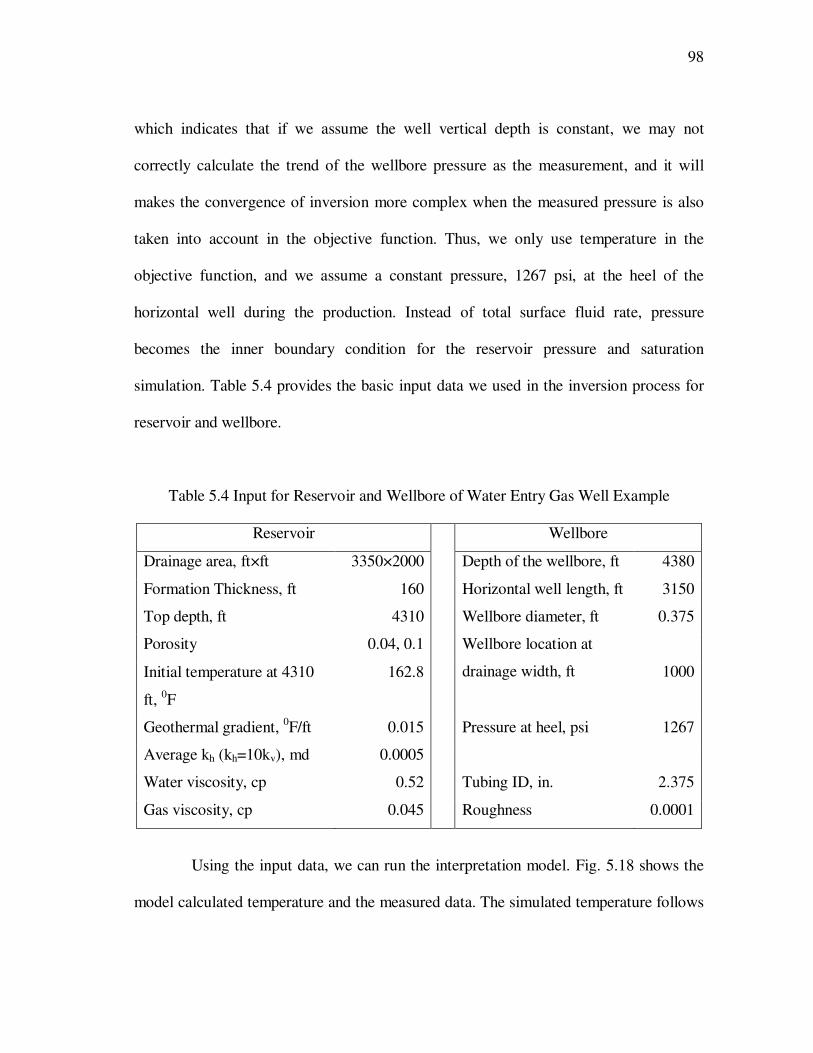
98

which indicates that if we assume the well vertical depth is constant, we may not

correctly calculate the trend of the wellbore pressure as the measurement, and it will

makes the convergence of inversion more complex when the measured pressure is also

taken into account in the objective function. Thus, we only use temperature in the

objective function, and we assume a constant pressure, 1267 psi, at the heel of the

horizontal well during the production. Instead of total surface fluid rate, pressure

becomes the inner boundary condition for the reservoir pressure and saturation

simulation. Table 5.4 provides the basic input data we used in the inversion process for

reservoir and wellbore.

Table 5.4 Input for Reservoir and Wellbore of Water Entry Gas Well Example

Reservoir Wellbore

Drainage area, ft×ft 3350×2000 Depth of the wellbore, ft 4380

Formation Thickness, ft 160 Horizontal well length, ft 3150

Top depth, ft 4310 Wellbore diameter, ft 0.375

Porosity 0.04, 0.1

Initial temperature at 4310

ft, 0F

162.8

Wellbore location at

drainage width, ft 1000

Geothermal gradient, 0F/ft 0.015 Pressure at heel, psi 1267

Average kh (kh=10kv), md 0.0005

Water viscosity, cp 0.52 Tubing ID, in. 2.375

Gas viscosity, cp 0.045 Roughness 0.0001

Using the input data, we can run the interpretation model. Fig. 5.18 shows the

model calculated temperature and the measured data. The simulated temperature follows

99

the trend of the observation. The major changes on the observed temperature curved are

captured by the forward-calculated-model. It means that the reservoir characterization

and water-gas distribution may be close to the true situation.

163.5

164

164.5

165

165.5

4600 5100 5600 6100 6600 7100 7600Measured depth, ft

Tem

pera

ture

, 0F

Calculated

Measured

Fig. 5.18 Calculated temperature matches the trend of measured data

At this temperature matching condition, we also obtain downhole flow

conditions. Fig. 5.19 provides the inverted gas and water flow rates in tubing, and Fig.

5.20 is the inverted permeability distribution. The interpretation result indicates that

water and gas mainly enter into the horizontal well at some small ranges, which may be

fracture locations.

From the interpretation we can see that there are at least three major fractures

along the horizontal well, with most likely the fracture at 7100 ft producing the highest

gas rate, and the other two fractures (at 5400 ft and 5900 ft) perform about the same.

Water is produced almost evenly along the fractures.

100

0

100

200

300

400

4600 5100 5600 6100 6600 7100 7600

Measured depth, ft

Flo

w r

ate

, M

scf/

d,

bb

l/d

Gas

Water

Fig. 5.19 Inverted flow rate distributions of gas and water

0.0001

0.001

0.01

0.1

1

4600 5100 5600 6100 6600 7100 7600

Measured depth, ft

Perm

eab

ilit

y,

md

Fig. 5.20 Inverted permeability distribution of water entry gas well example

101

5.2 OPTIMIZE HORIZONTAL WELL PERFORMANCE BY INFLOW

CONTROL VALVE FROM TEMPERATURE FEEDBACK

Downhole flow conditions are key information to optimize well performance. Recently,

intelligent completions, such as inflow control valves (ICV) or inflow control devices

(ICD), have been used to operate well performance based on downhole flow conditions

or production data. Many studies have been presented in analyzing these data for

production optimization. Alaeddin and Maizeret (2003) used production logging

technology to evaluate the contribution of two horizontal legs and possible water entry

locations. This information can help to manage reservoir for optimizing the re-

development plan of the field. Real time production data is also used for optimizing oil

recovery in multilateral wells (Alghareeb et al., 2009). Based on the production history

data and reservoir permeability distribution, an optimum ICV configuration can be

obtained so as to minimize water cut and maximize net present value. Qing and Davies

(2009) presented a generalized predictive control for management of ICVs by production

feedback update. Alhuthali et al. (2007) provided an optimal waterflood reservoir

management by rate control. Their results show that the correct rate control for

horizontal well with ICV completions can delay water breakthrough and significantly

increase the reservoir recovery for a heterogeneous reservoir.

Much of the previous optimization works are based on assumed reservoir

geologic models. Then, the downhole flow condition in horizontal wells can be predicted

via forward modeling. However, in some situations, reservoir geologic models may not

be available, or not exact enough to predict correct downhole flow conditions.

102

Production history matching is routinely used to update geologic models. But some

important production data, such as water cut history, is useful when water breakthrough

is observed. On the other hand, some optimized operations may achieve good result

when they are used at the beginning of the well producing (Alhuthali et al., 2007).

In the previous chapter, it was concluded that downhole temperature data in

horizontal well can reflect the inflow rate distribution. The transient temperature

behavior can be measured by downhole permanent sensors such as distributed

temperature sensor (DTS) throughout the lifetime of the well, which means that we

probably can obtain downhole flow conditions at very early time.

Flow profile along a horizontal well strongly depends on the heterogeneity of

the reservoir that is connected to the wellbore. Non-uniformly distributed flow in a

horizontal well usually causes production problems such as early water or gas

breakthrough at high permeability zones. Rather than wait until the well starts producing

water or gas, it is suggested to use temperature distribution data as an indicator to locate

the problem zones, and to operate ICVs to delay the early breakthrough. The purpose of

this work is to use inflow control valves (ICV) to relocate the inflow distribution

according to temperature feedback at early time of a well producing life when a reliable

reservoir geologic model is not available. The inflow rate distribution in horizontal wells

may achieve an optimized condition when the arriving time of fluid along a horizontal

wellbore close to uniform distribution. At such a condition, oil production will be

improved with delayed water/gas breakthrough.

103

5.2.1 Application Procedure of Temperature Feedback

Realized that the uniformed flow rate distribution does not necessarily mean uniformed

temperature distribution because of heat transfer while flowing through the reservoir, we

first need to identify the permeability field, and then find the desired temperature profile

that corresponds to the uniformed flow distribution, and finally operating ICVs to

achieve the optimal condition. Fig. 5.21 shows this procedure. It includes the following

steps:

1. Start from an initial condition that assumes all ICVs are fully open.

2. Observe temperature distribution outside of ICVs. According to the measured

data, estimate the inflow rate distribution along horizontal well, and identify the

high inflow sections.

3. Establish a desired temperature distribution which yields an approximate optimal

production condition. Estimate the flow rate change based on the temperature

distribution.

4. Operating ICVs until the desired temperature distribution is achieved.

104

Fig. 5.21 Optimization procedure of operation on ICV from temperature feedback

ICV Effects on Temperature Behavior

The simulation on temperature behavior in horizontal well has been discussed in

previous sections. If the horizontal well is equipped by ICVs, the ICV effect on

temperature behavior should be considered. Muradov and Davies (2008, 2009)

developed a temperature model for the wells with ICVs. They considered that the

temperature effect of ICV is caused by pressure drop when fluid passes through the ICV.

This temperature change can be calculated by the relation of Joule-Thomson effect:

Start

Horizontal well produces, all ICVs are open

Observe temperature outside of ICVs; Estimate permeability and inflow rate distribution from

temperature interpretation model

End

Calculated desired temperature profile based on permeability

field for uniform flow rate

Operate ICVs and monitor temperature until it is close to the

desired temperature profile

105

pKCT JTD ∆=∆ 2 ............................................................................................ (5.1)

where p∆ is the pressure change when the fluid pass through the ICV, JTK is the average

Joule-Thomson effect if the fluid is multiphase, and DC is a valve discharge coefficient,

and it is assumed to 1 in this chapter. It has a relation with the nozzle efficiency defining

for ICV flow model, and can be found in the work of Muradov and Davies (2008).

When ICVs are installed, it causes an additional pressure drop when fluid flow

through, which results in a corresponding temperature change. That is illustrated in Fig.

5.22.

Fig. 5.22 ICV effect on pressure distribution and temperature in our model

As ICVs close up to control the flow rate, it causes an additional pressure drop.

Generally, the pressure drop through ICVs, ICVp∆ is relative to the flow rate passing

through the equipment (Perkins, 1993). However, this pressure drop may not be

Linear section

with ICVs

DTS

Pres

pwf

∆pIC

V

∆pdrawdown w/o

∆TICV

∆pdrawdown, w/ICV

106

measured, and it leads to an unknown inflow flux through the ICV. In reality, we might

not know the amount of flow rate through the ICV when we make changes to it.

Therefore, in the synthetic case shown here, a reasonable additional pressure was added

to the inflow performance relationship for reservoir and wellbore connection. When we

solve the reservoir pressure equation, the general sink/source term is modified to:

( )( )jwgridjj pppPIq ∆+−= ......................................................................... (5.2)

where PI is the productivity index for the well presented by Peaceman (1983).

The Designed Temperature Distribution

The target is to achieve the condition where the arriving time of reservoir fluids along a

horizontal well is close to a uniform distribution. This is hard to accomplish because we

may not know the detailed reservoir description. We can use the arriving temperature to

establish the permeability distribution, and then use it as a reference to regulate arriving

time of fluid. For high inflow locations, we want to use ICVs to reduce the influx, and

for low inflow locations, we assign ICVs to fully open to keep the maximum influx rate.

The question is how this uniform distribution can be reflected by temperature

information.

Once we understand the flow distribution without ICV regulation, we know, if

ignore the pressure drop in horizontal well, the pressure drawdown distributions from

reservoir to wellbore are the almost the same along the wellbore, with higher-

permeability zones getting higher inflow rate and lower-permeability zones lower inflow

rate. If ICVs are fully open, for oil reservoirs, temperature at higher-perm location will

107

be higher than the rest of wellbore location. Since using ICV to choke back flow rate

generate additional pressure drop and more frictional heating (Fig. 5.22), an ideal

temperature distribution should have lower temperature at higher-permeability locations.

We can estimate this desired temperature distribution based on the permeability

distribution we obtained from temperature assessment, and then operate ICVs to achieve

the optimal condition. Most ICVs used in the field today have discontinuous operating

positions (e.g., two-position: open/close, three-position: open/50% open/close, etc.). It is

difficult to set exactly the ideal condition. To apply the method practically, we would

gradually operate the ICVs and watch the temperature change to approach the desired

condition. The following examples illustrate the procedure.

5.2.2 Bottom Water Driving Reservoir

The horizontal well structure used for this example is shown in Fig. 5.23, and Fig. 5.24

shows the reservoir geometry and the 2D permeability distribution. The horizontal well

is 3000 ft long, equipped with ICVs at certain completed sections. The well is divided

into 10 sections, each has 100-ft perforated zone with an ICV, and 200-ft blank section.

The well is located at the middle of reservoir. A strong aquifer is at the bottom of the

reservoir. The reservoir has a high permeability strip (200 md) at around 2000-ft

location, with the permeability about four times of the average reservoir permeability (50

md). The input information for the reservoir and well system are in Table 4.1, and the

fluid and rock thermodynamic properties are in Table 3.2.

108

Fig. 5.23 Horizontal well structure

X

Y

0 500 1000 1500 2000 2500 3000

0

500

1000

1500

2000

40 80 120 160 200PERMX

Fig. 5.24 Reservoir geometry and 2D permeability distribution

The temperature distribution in Fig. 5.25 is recorded outside of ICV at 0.5 day

and 2 days, and the corresponding oil flow rate profile along the wellbore translated

from the initial temperature data. During this period, all ICVs are fully open, and

therefore they do not affect the temperature behavior. We observe a high temperature

section from 1900 to 2100 ft. The previous study can translate this temperature profile to

a flow rate distribution, shown in Fig. 5.26. This higher temperature is caused by a

higher inflow rate which leads to a faster transient temperature increasing compared with

the rest of the wellbore.

109

170.2

170.4

170.6

170.8

171

0 800 1600 2400 3200Well distance from heel, ft

Tem

pera

ture

, 0F

2 days

0.5 day

Initial, Identify high

inf low rate

Fig. 5.25 Use temperature to identify high inflow rate before operating ICVs

0

4

8

12

16

20

0 800 1600 2400 3200Well distance from heel, ft

Flo

w r

ate

, b

bl/d

/ft

Fig. 5.26 Flow rate profile before operating ICVs

With this initial condition, we are ready to adjust the ICVs at 1900 to 2100 ft

section to reduce the inflow rate. ICVs are designed as 2-position ICVs (open/close), 3-

110

position ICVs (open/50% open/close), 4 position ICVs, etc. When an ICV is operated to

open or close at certain position, the pressure drop corresponding to the operation is

unknown, so does the flow rate change. The relationship, as mentioned before, depends

on individual ICV design. To include the effect of ICVs in the simulation, Eq. 5.2 is

equal to,

( )jwgridjj ppPIq −⋅= γ ............................................................................... (5.3)

where γ is defined as a choking ratio for ICV, and [ ]1,0∈γ . Then the equivalent

pressure drop p∆ is calculated by

))(1( wgrid ppp −−=∆ γ ................................................................................ (5.4)

and p∆ is further used to calculated temperature. Fig. 5.27 is the choking ratio

distribution which will be used in the following calculation.

0

0.25

0.5

0.75

1

0 800 1600 2400 3200Well distance from heel, ft

Ch

okin

g r

ati

o f

or

each

IC

V

First operation

Second operation

Third opertation

Fig. 5.27 Choking index ratio changes in simulation at different ICV stages

111

Suppose we start operating the ICVs at the end of 2 days of production. In this

operation, γ is set to 0.75. But we do not know how much pressure drop it generates,

and how much inflow fluid passes through the ICVs. Therefore, we use temperature

feedback to analyze whether the operation achieves the optimal design. Fig. 5.28 is the

observed temperature that is much less uniformed distributed along the wellbore after we

control the ICVs. According to the procedure, this temperature distribution most likely

does not meet our design requirement for optimization. Temperature at high inflow rate

section still increases faster than other sections, which means the inflow rate here is still

higher than the optimal design requires. Therefore, we need to further control the ICV.

It also shows that the temperature feedback is not instantaneous. It takes days to

see whether the temperature at this location still increases faster. This is because of the

formation heat resistance, which is a significant effect on the transient temperature

behavior

170.2

170.4

170.6

170.8

171

0 800 1600 2400 3200

Well distance from heel, ft

Tem

pera

ture

, 0F

4 days

2.5 daysevenly distributed temperature

Fig. 5.28 Observe temperature feedback after controlling ICV at high inflow section

112

At 4.5 days, ICV is operated again with =γ 0.5, Fig. 5.29 shows the result of

temperature and Fig. 5.30 gives the flow rate profiles. Temperature has reached the

stable status, but the corresponding rate is still much higher at the high-permeability

zone, which indicates that further choking is required at this moment.

170.2

170.4

170.6

170.8

171

0 800 1600 2400 3200Well distance from heel, ft

Tem

pera

ture

, 0F

6 days

4.5 days

high rate location

Fig. 5.29 Temperature achieves design at first adjustment

113

0

2

4

6

8

10

0 800 1600 2400 3200Well distance from heel, ft

Infl

ow

rate

, b

bl/d

/ft

Fig. 5.30 Inflow rate distribution at first adjustment

To achieve a uniform inflow rate distribution in wellbore, the original inflow

rate, 16 bbl/d/ft, should be reduced close to 4 bbl/d/ft of other section, as shown in Fig.

5.26. Then the estimated choking off rate at the identified high permeability section is

about 0.75 of the original rate. Although the relation between ICV position and flow rate

is not linear, we can use this as a guideline. We applied this amount to the ICV (set

=γ 0.25) and let the temperature transient effect to settle down to reach the equilibrium.

Fig. 5.31 and Fig. 5.32 show the inflow rate distribution at this status, the temperature

stabled at the desired profile, and the flow rate is satisfied as much more even

distribution along the wellbore is achieved.

114

170.2

170.4

170.6

170.8

171

0 800 1600 2400 3200

Well distance from heel, ft

Tem

pera

ture

, 0F

8 days

6.5 dayssatisfied temperature

Fig. 5.31 Second ICV operation to meet the desired temperature

0

2

4

6

8

10

0 800 1600 2400 3200

Well distance from heel, ft

Infl

ow

rate

, b

bl/d

/ft

Fig. 5.32 Inflow rate is closed to evenly distribute

The daily oil rate is shown Fig. 5.33, and Fig. 5.34 shows the bottomhole

pressure changes as a function of producing time at three conditions: no ICV choking,

115

initial adjustment with even temperature, and final adjustment with even flow rate.

Notice that even though the inflow rate distribution at the final adjustment is closer to

the uniform and the higher rate is choked back, its total oil rate is a little higher than the

one without ICV control. The procedure of optimizing production by ICVs delayed

water breakthrough, as well as increased daily oil rate.

1000

2000

3000

4000

5000

0 150 300 450 600 750 900

Time, days

Oil r

ate

, S

TB

/d

Even flow rate

Even temperature

w ithout ICV control

Fig. 5.33 Daily oil rate vs. time at three conditions

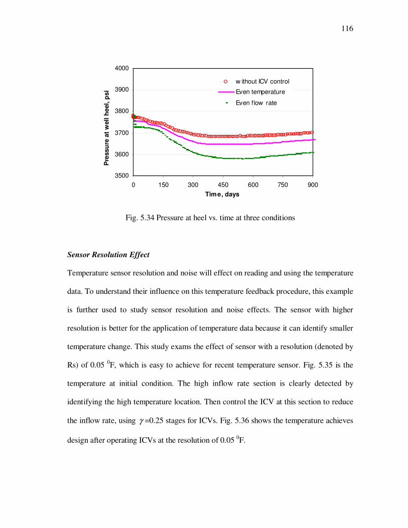
116

3500

3600

3700

3800

3900

4000

0 150 300 450 600 750 900

Time, days

Pre

ssu

re a

t w

ell h

eel, p

si

w ithout ICV control

Even temperature

Even flow rate

Fig. 5.34 Pressure at heel vs. time at three conditions

Sensor Resolution Effect

Temperature sensor resolution and noise will effect on reading and using the temperature

data. To understand their influence on this temperature feedback procedure, this example

is further used to study sensor resolution and noise effects. The sensor with higher

resolution is better for the application of temperature data because it can identify smaller

temperature change. This study exams the effect of sensor with a resolution (denoted by

Rs) of 0.05 0F, which is easy to achieve for recent temperature sensor. Fig. 5.35 is the

temperature at initial condition. The high inflow rate section is clearly detected by

identifying the high temperature location. Then control the ICV at this section to reduce

the inflow rate, using γ =0.25 stages for ICVs. Fig. 5.36 shows the temperature achieves

design after operating ICVs at the resolution of 0.05 0F.

117

170.2

170.4

170.6

170.8

171

0 800 1600 2400 3200Well distance from heel, ft

Tem

pe

ratu

re,

0F

2 days

0.5 day Identify high inflow rate

Rs = 0.05 0F

Fig. 5.35 Identify high inflow sections at initial, Rs = 0.05 0F

170.2

170.4

170.6

170.8

171

0 800 1600 2400 3200Well Distance, ft

Tem

pe

ratu

re,

0F

8 days

6.5 day

Rs = 0.05 0 F

satisf ied temperature

Fig. 5.36 Temperature achieves design, Rs = 0.05 0F

If the sensor with a resolution of 0.1 0F, the temperature at 0.5 day can not be

used to identify high inflow rate section, as shown in Fig. 5.37. Fig. 5.38 shows that the

temperature distribution at 1 day still can not be used.

118

170.2

170.4

170.6

170.8

171

0 800 1600 2400 3200Well distance from heel, ft

Tem

pera

ture

, 0F

0.5 day

high inf low rate can not be identified correctly

Rs = 0.1 0F

Fig. 5.37 Unable to identify high inflow sections at 0.5 day, Rs = 0.1 0F

170.2

170.4

170.6

170.8

171

0 800 1600 2400 3200Well distance from heel, ft

Tem

pera

ture

, 0F

1 day

high inflow rate can not be identified correctly

Rs = 0.1 0F

Fig. 5.38 Unable to identify high inflow sections at 1 day, Rs = 0.1 0F

The temperature data observed at 2 days may be used to identify the high inflow

rate, as shown in Fig. 5.39. Operation of ICVs is not applied because the sensor with a

resolution of 0.1 0F is not very successful to identify high inflow rate section.

119

170.2

170.4

170.6

170.8

171

0 800 1600 2400 3200Well distance from heel, ft

Tem

pera

ture

, 0F

2 days high inf low rate

Rs = 0.1 0F

Fig. 5.39 May identify high inflow sections at 2 days, Rs = 0.1 0F

Noise Effect

The noise of the sensor has bigger effect on the result of the procedure. A normal

distribution of noise is introduced to exam its effect on the temperature application. The

noise is with zero mean and a variance of σ. Fig. 5.40 shows the temperature at initial

condition, and its feedback after ICV operation when the noise variance is 0.033 0F. The

higher temperature zone indicates the higher inflow zone before and after operating the

ICVs by temperature feedback, showed in Fig. 5.41. The result shows that the

optimization can be applied at this noise level.

120

170.2

170.4

170.6

170.8

171

0 800 1600 2400 3200Well distance from heel, ft

Tem

pera

ture

, 0F

2 days

0.5 dayInitially identify high rate

σ = 0.033 0F

Fig. 5.40 Identify high inflow sections at initial, σ = 0.033 0F

170.2

170.4

170.6

170.8

171

0 800 1600 2400 3200Well distance from heel, ft

Tem

pera

ture

, 0F

6 days

4.5 days

first adjustment even

temperature

σ = 0.033 0F

Fig. 5.41 Temperature achieves design, σ = 0.033 0F

When the noise variance is 0.1 0F, the temperature distribution in wellbore are

shown Fig. 5.42 and Fig. 5.43. The result shows that the temperature data fails to detect

121

inflow rate distribution correctly at this noise level. The procedure cannot be used in this

situation.

170

170.2

170.4

170.6

170.8

171

0 800 1600 2400 3200

Well distance from heel, ft

Te

mp

era

ture

, 0F

0.5 day

σ = 0.1 0F

Fail to identify high rate

Fig. 5.42 Failure to identify high inflow sections at 0.5 day, σ = 0.1 0F

170

170.2

170.4

170.6

170.8

171

0 800 1600 2400 3200Well distance from heel, ft

Tem

pe

ratu

re,

0F

5 days σ = 0.1 0F

Fail to identify inf low rate

Fig. 5.43 Failure to identify high inflow sections at 5 day, σ = 0.1 0F

122

5.2.3 Water Injection in Channel Formation

For the channel formation, Fig. 5.44 shows the reservoir geometry and the 2D

permeability distribution which is generated by FLUVSIM (Deutsch and Tran, 2002).

The reservoir has an average permeability of 50 md, with a channel in the reservoir only

connecting the injector. The channel permeability is 700 md, which may be detected by

openhole logging. However, it does not cross with the production well. We may not

know the exact structure of this channel in the reservoir.

The reservoir thickness is 50 ft, and the production well and the injection well

are located at the middle of the reservoir thickness. The producing well has a constant

total liquid rate of 4000 bbl/day initially, and the injection well is at constant pressure

4000 psi, and the injected water temperature is 100 0F.

The same as the previous example, we assumed that the well has 10 sections.

Each section has an ICV and a blank pipe to isolate reservoir inflow. Each section is

300-ft long, as shown in Fig. 5.23. Other inputs are kept the same as the previous

example.

123

X

Y

0 500 1000 1500 2000 2500 3000

0

500

1000

1500

2000

0 200 400 600 800

PERMX

Fig. 5.44 Reservoir geometry and 2D permeability distribution used in example 2

The first step is to use temperature to identify high inflow rate sections. Fig.

5.45 shows the temperature behavior of the producing well. The temperature does not

reflect the rate distribution at early time (0.5 days), and the high-temperature section

becomes more obvious at 10 day. Thus, we detect the high inflow section from 0 to 1500

ft. The level of temperature increase along the section of 0 to 1500 ft is different, and the

inflow rate from 700 ft to 800 ft is the highest. Fig. 5.46 shows the interpreted flow rate

profile at initial condition without regulation by ICVs. The permeability heterogeneity

will result in an early breakthrough of injected water first at the location of 700 ft to 800

ft, then the entire 1500 ft region towards the heel of the well. This study is to operate the

ICVs at the section from 0 to 1500 ft, and monitor the temperature feedback. The

adjustment on ICV at each section is different, depending on the observation from the

temperature distribution at 10 days. For example, at the range with the highest initial

temperature (700-800 ft), it is expected to have a lower temperature than other section

after control; and temperature at other sections in the first 1500 ft would be a little higher

124

than the temperature at 700 - 800 ft section. Thus, the choking ratio γ is the lowest, γ is

gradually increasing towards the toe, and γ is one (no choking) from 1800 to 3000 ft.

Fig. 5.47 shows the change of ICV position along the wellbore.

170

170.4

170.8

171.2

171.6

0 800 1600 2400 3200Well distance from heel, ft

Tem

pera

ture

, 0F

10 days

0.5 day

identify high rate

Fig. 5.45 Use temperature to identify inflow rate distribution

0

2

4

6

8

10

0 800 1600 2400 3200Well distance from heel, ft

Flo

w r

ate

, b

bl/

d/f

t

Fig. 5.46 Inflow rate distribution before operating ICV

125

0

0.25

0.5

0.75

1

0 800 1600 2400 3200Well distance from heel, ft

Ch

okin

g r

ati

o f

or

each

IC

V50%

25%

75%

Fig. 5.47 Choking index ratio changes along wellbore

Because the ICV stages are discontinuous, they cannot be set as an arbitrary

value. The temperature distribution in Fig. 5.48 does not achieve the desired

temperature using the stages in Fig. 5.47. But compared with Fig. 5.45, it is improved.

Fig. 5.49 shows that the flow rate distribution along the wellbore at this ICVs setting

condition is much more evenly distributed.

126

170

170.4

170.8

171.2

171.6

0 800 1600 2400 3200Well distance from heel, ft

Tem

pera

ture

, 0F

14 days

24 days

Temperature not satisf ied,

but improved

Fig. 5.48 Temperature after ICV operation

0

2

4

6

8

10

0 800 1600 2400 3200Well distance from heel, ft

Infl

ow

rate

, b

bl/d

/ft

Fig. 5.49 Inflow rate distribution after ICV operation

The procedure presented in this paper helped to improve the well performance.

It is realized that we can install ICVs on either or both producing well and injecting well.

127

Fig. 5.50 shows the predicted inflow rate for this example, including production without

ICVs, production with ICVs only on the producer, and production with ICVs on both the

producer and the injector. The ICVs setting stages for producing well are mentioned

above. At the cross of the channel and the injecting well, the ICVs on injecting well is

set to γ =0.25, which tries to reduce the water comes through the channel.

It is clear that ICVs on the producer is considerably beneficial compared with

no ICVs at all. Oil production rate improved significantly in additional to delayed water

breakthrough. With the initial temperature information, we may be able to detect the

connection between the channel and the injector at 1760 ft to 2000 ft. But meanwhile,

adding more ICVs on the injector at this location to control the injection rate does not

yield enough further improvement to the production. If considering the complication,

cost and risk involved, this is probably not recommended.

2000

3000

4000

5000

0 200 400 600 800 1000

Time, days

Oil r

ate

, S

TB

/d

Without ICVs

ICVs on

producer only

ICVs on

Producer and

injector

Fig. 5.50 Daily oil rate shows the production improvement

128

5.3 TEMPERATURE MEASUREMENT ASSISTS RESERVOIR

CHARACTERIZATION

Most permeability fields contain certain geostatistical characteristics that are much more

complicated than just a 1D variation, as shown in Chapter III. However, in Chapter III,

the temperature inversion process results in a very coarse-scale estimate of the reservoir

permeability distribution. This coarse-scale permeability can cause significant deviation

on prediction of reservoir and well performance. For example, from Fig. 4.38, we can

see that the simulated water-cut history with the inverted permeability distribution

follows the trend of the observed data, but contains a significant mismatch. We can also

see that the inverted temperature at the high permeability section increases faster than

the observed data (Fig. 4.34). Some of these discrepancies arise from the fact that the

inverted permeability is only 1D, which is an approximation of the true 2D permeability

field.

Production histories, such as water cut and oil rate, can be collected at the

surface. This history data is generally used to update reservoir characteristic. Recently,

geologically-based history matching of production data has been used to improve the

understanding of reservoir permeability field. A number of techniques have been

reported in the literature. Integration of production data typically requires the

minimization of a predefined objective function, which consists of data difference

between observed and simulated production responses and penalty terms, which preserve

the prior information and prevent rough changes. The streamline generalized travel time

inversion technique has been proven to be an efficient means for computing parameter

129

sensitivities ( Datta-Gupta et al., 2001; Cheng et al., 2004). This technique uses an

analytical approach that involves 1D integral along streamlines to efficiently compute

the parameter sensitivities using a single forward simulation, which can be either a

streamline or a finite-difference simulator. This kind of history matching approach has

been utilized in a large number of field applications (Cheng et al., 2005; Hohl et al.,

2006; Rey et al., 2009).

Based on these techniques, we try to generate a high-resolution permeability

model, including both temperature and production history information. A coarse-scale

permeability distribution is obtained by temperature interpretation, as discussed in

Chapter III. Then, the coarse-scale permeability is used as constraints in generating high

resolution geological models using geostatistical method, sequential Gaussian simulation

with block kriging. Finally, these models are calibrated to production data using

streamline-based generalized travel time inversion.

5.3.1 Integrated Approach of Temperature and History Matching

The objective is to incorporate temperature information into geologic modeling and

production history matching to better characterize the reservoir. There are two potential

approaches, possibly among others. The first one is to incorporate the coarse-scale

permeability information as ‘secondary’ information while constructing the prior

geologic model. This model can then be history matched to further update the geologic

model. Another approach would be to include the temperature-derived coarse-scale

130

permeability as a penalty function during the history matching process. The former

approach is used here.

The outline of an integrated approach is shown in Fig. 5.51. It combines the

temperature interpretation and production history matching for dynamic reservoir

characterization and modeling. It includes four major steps as follows:

1. Use of temperature interpretation method to match the observed temperature

data, and obtain a coarse-scale permeability distribution.

2. Generating high-resolution geologic model constrained to the coarse-scale

permeability estimate. This is accomplished using sequential Gaussian simulation

with block kriging, much along the line of seismic data integration into geologic

models.

3. Use of the geologic model from step 2 as the prior model for production history

matching. The history matching is carried out using a fast streamline-based

approach.

4. Use the forward model of wellbore temperature to cross-check that the history

matched model reproduces the temperature data. If the updated model reproduces

the wellbore temperature measurements within pre-specified tolerance, we accept

the refined permeability distribution. Otherwise, we go back to step 2 and repeat

the process.

131

Fig. 5.51 Integrated approach for incorporating temperature data into history matching

5.3.2 Downscaling Method

The objective is to obtain a 2D fine-scale permeability distribution from the 1D coarse-

scale permeability which is generated from the temperature inversion. Fig. 5.52 helps us

to understand the purpose of this downscaling. In the downscaling process, the known

values are the coarse-scale permeability (Fig. 5.52 a). The near wellbore permeability

may be also obtained after the openhole logging, for example, permeability can be

calculated using porosity provided by openhole logging. The unknown values need to be

Step2: Downscale the coarse-scale permeability by sequential

Gaussian simulation with block kriging

Finish

Step3: Updating permeability by a fast history matching method based

on streamline sensitivity calculation

Temperature data

still match?

Yes

No

Step1: temperature interpretation, obtain a coarse-scale

perm distribution

132

determined are the permeability in each reservoir grid, which construct the fine-scale

permeability, as shown in Fig. 5.52 b.

a b

Fig. 5.52 Downscaling of the temperature inverted coarse-scale permeability

Kriging

In geostatistics, kriging is the estimation procedure using known values and location

information to determine unknown values. We use Fig. 5.53 to illustrate the kriging

estimation. Suppose permeabilities at points 1 and 2 are known, and they are 100 md and

200 md respectively. Permeability at point 0 is unknown and need to be determined. The

distance, 5010 =l ft, 10020 =l ft, and 13012 =l ft.

Fig. 5.53 Simple example for kriging estimation

The permeability, 0k , can be linearly estimated from known value, 1k , and 2k by

1 2

0

l20 l10

l12 130 ft

100 ft 50 ft

downscale

133

( ) mkkk ⋅−−++= 2122110 1 λλλλ ................................................................... (5.5)

where 1λ and 2λ are weights, and m is mean of 0k .

For 1λ and 2λ , they are calculated by

( ) ( ) ( )( ) ( ) ( )20222121

10122111

lll

lll

γγλγλ

γγλγλ

=⋅+⋅

=⋅+⋅........................................................................ (5.6)

where γ is a semi-variogram, which can reflect the influence of locations between

points. It can be adopted by different models. For example, γ can be given

mathematically as

( )

≥

<

−

=

alc

ala

l

a

lc

l 3

3

2

1

2

3

γ ................................................................... (5.7)

where c and a are constants which are determined by the known values (samples). This

relation is spherical model. For simplification, these constants are set as 1=c , a =150 ft.

There are many types of kriging based on how to solve Eq. 5.5. For simple

kriging, the mean, m , must be known. For example, if we assume m =100, then using

Eq. 5.7 with the distance 5010 =l , 10020 =l , and 01122 == ll , 13012 =l , we can get

( ) ( ) 02211 == ll γγ , ( )12lγ =0.9745, ( ) =10lγ 0.4815, ( ) =20lγ 0.8519. Then substituting

these values into Eq. 5.6, we get =1λ 0.8742, =2λ 0.4941. Finally, the permeability,

0k can be obtained by Eq. 5.5, 0k =149 md.

134

For ordinary kriging, 121 =+ λλ is a constraint, the mean, m , is not necessary.

This constraint is solved with modified Eq. 5.6 by introducing an unknown, η , called

Lagrange multiplier. Then Eq. 5.6 becomes

( ) ( ) ( )( ) ( ) ( )20222121

10122111

lll

lll

γηγλγλ

γηγλγλ

=+⋅+⋅

=+⋅+⋅.................................................................. (5.8)

The solution for 1λ and 2λ are 1λ =0.69, 2λ =0.31. Therefore, 0k =131.

In the same time, for ordinary kriging, an estimation variance, 0σ , of this point can

be calculated by

( ) ( )202101

2

0 ll γλγλσ += ................................................................................ (5.9)

It indicates that the estimated value, 0k , should follow a normal distribution.

Reservoir grid can be treated as a block because it is a 3D object. Therefore,

block kriging, which estimates the value of a block property from a set of nearby known

values using kriging, is used in the downscaling. The estimation procedure is similar to

the procedure above.

Sequential Gaussian Simulation

Generally, the result from kriging is very smooth. It may underestimate the

heterogeneity. And the kriging result is deterministic. For unknown permeabilities, they

may not be determined with certainty. Using stochastic method to describe them may be

more reasonable. Therefore, the sequential simulation method with kriging is commonly

used in geologic modeling. Because Gaussian (normal) distribution is the most popular

135

distribution in statistic, sequential Gaussian simulation with block kriging (Behrens et

al., 1998) is used for downscaling in this study.

Suppose the reservoir permeability model has 0N known values at initial, the

sequential Gaussian simulation is performed as following steps:

1. Randomly select a reservoir grid, A1.

2. Perform the kriging procedure based on the 0N values, obtain an estimated

value, *

1k , for the selected grid, and its variance, 1σ . Then randomly generate 1k

from normal distribution ( )2

1

*

1 ,σkN , and set this 1k to the reservoir grid, A1.

3. Include 1k to the known values, then it has 0N +1 values. Based on this

condition, repeat step 1 and 2, until all interested grids are completed.

After these steps, the sequential Gaussian simulation will generate a

permeability distribution based on the known values.

In this study, the coarse-scale permeability distribution from temperature

inversion, and permeability near wellbore are known values. The first one is treated as

block data, and the second one is treated as point. The kriging estimator, SKZ ,

conditioned to both point data and block data (Liu and Journel, 2009) is:

DmuT

SKZ Λ+= 0)( ...................................................................................... (5.10)

where u means the point which need to be estimated. 0m denotes stationary means, and

it is a known value. ],[ BPD =T denotes the known data value vector, P denotes data

points, B denotes block data, ],[BP

Tλλ=Λ denotes the kriging weights for point data P

and block data B. And it can be calculated similar to Eq. 5.6.

136

With this method, the coarse-scale permeability is downscaled and the fine-

scale permeability distribution is assigned to reservoir grids. And it also includes the

permeability information near wellbore.

5.3.3 Production History Matching

The fine-scale permeability distribution derived from downscaling is now further

updated by history matching of production data. This step involves minimization of a

least-square difference between the observed data and the calculated response with

additional constraints by prior model. In this approach, we have adopted the streamline

generalized travel time inversion for history matching, primarily because of its

computational efficiency and quasi-linear properties (Cheng et al., 2005).

Suppose the water-cut history is observed, showing in Fig. 5.54 marked with

triangles. The water-cut from initial permeability is calculated, showing in Fig. 5.54

marked as the circle in front of the observed data curve. The history matching method is

to find an optimal time-shift to minimize the production data difference between

observation data and calculated response. It only shifts the initial calculated water-cut

history parallelly without changing its shape.

For a well of interest, the optimal shifted time can be obtained from the

coefficient of determination, which is given by

137

[ ]

[ ]∑

∑

−

∆+−

−=∆

i

obs

i

obs

i

i

cal

i

obs

yty

ttyty

tR2

2

2

)(

)()(

1)( ...................................................... (5.11)

where y is the water cut. The only variable in Eq. 5.11 is t∆ , which is the time used to

shift the initial calculated water cut. The value of t∆ leading the maximum 2

R is called

the optimal shifted time, denoted by t~

∆ . The left plot in Fig. 5.54 shows that with t~

∆ ,

the shifted water cut is most close to the observed water cut. The right plot shows the

coefficient of determination,2

R , as a function of t∆ , and for t~

∆ , 2

R has the maximum

value.

Fig. 5.54 Illustration of generalized travel time difference and correlation function

(Cheng et al., 2004)

Once the optimal shifted time t~

∆ is obtained, the next step is to change

reservoir parameters to get the new calculated water cut, which is better matching the

observed data. In this work, reservoir permeabilities are the parameters to be changed.

The changing permeabilities can be determined by

138

0~

=−∆ kSt δ ............................................................................................. (5.12)

where S is the sensitivity of shifted time with respect to permeability,

k

tS

∂

∆∂=

~

....................................................................................................... (5.13)

A critical aspect of production data integration is efficient computation of the

sensitivities. We used a streamline-based approach to compute these sensitivities (Cheng

et al., 2005; Datta-Gupta and King, 2007). Recall Eq. 2. 23, for two-phase

incompressible flow of oil-water in a nondeformable, permeable medium, the transport

equation can be written in the streamline time-of-flight coordinates as follows:

0=∂

∂+

∂

∂

τww F

t

S............................................................................................. (5.14)

where τ represents time of flight which is the travel time along a streamline,

ψ , and s(x)

is the “slowness” defined as the reciprocal of the total interstitial velocity

∫=ψ

τ dxs )(x .................................................................................................. (5.15)

pks

rt ∇==

λ

φ

)(

1)(

xvx ................................................................................ (5.16)

where x is the reservoir grid where the streamline pass through. From Eq. 5.16, we have

k

s

pkk

s

rt

−=∇

−=∂

∂

λ

φ2

1............................................................................... (5.17)

Because changes in reservoir properties are small, it is assumed that streamline paths do

not shift significantly. Then, the change in travel time is related to the change in

reservoir properties and thus slowness by

139

∫∫∫

∂

∂+−=

∂

∂+

∂

∂==

ψψψ

δφφ

δδφφ

δδδτ dxs

kk

sdx

sk

k

sdxs )(x ..................... (5.18)

In this work, the effective permeability is parameter to calibrate, therefore,

0=δφ , and Eq. 5.18 becomes

( )( )( )∫

∑

−= dxk

s

dk

d

x

x

x

τ..................................................................................... (5.19)

which can be further related to arrival time of water front by

dk

dt

k

t τ

τ∂

∂=

∂

∂................................................................................................. (5.20)

According to Eq. 5.14, and wF is only a function of wS , it can be derived that

www

w

dSdFF

St

/

1−=

∂

∂−=

∂

∂

τ............................................................................ (5.21)

Therefore, the sensitivity along one streamline can be calculated by integrating

the “slowness” from the reservoir grids where the streamline pass through

( )( )∫

∑

=−=∂

∂=

∂

∂dx

k

s

dSdFdk

d

dSdFdk

dt

k

t

wwww x

x

/

1

/

1 ττ

τ................................... (5.22)

The overall sensitivity can be calculated by averaged sensitivities for all

contributed streamlines at all time steps. Therefore, the sensitivity S is:

k

t

k

t

∂

∂−=

∂

∆∂=

~S ........................................................................................... (5.23)

Now the sensitivity S can be used in the production data integration. During

this integration, we also want to preserve the initial permeability, and the permeability

140

changes should be smooth. But Eq. 5.12 cannot achieve this purpose. Therefore, a

penalized difference function, k)f(δ , is given below

kLkkSt k)f( δβδβδδ 21

~++−∆= .......................................................... (5.24)

The permeability change, kδ , leading a minimum of k)f(δ , will be adding to

the prior permeability in this history matching method. In Eq. 5.24, the first term is the

data misfit as quantified by the generalized travel time shift, the second the term is the

norm penalty and the third term is the roughness penalty. The norm penalty minimizes

the changes to the prior model that already incorporates well and geologic data and also

the coarse-scale permeability derived from the temperature data. The roughness penalty

ensures that the changes to the model are smooth and large-scale consistent with the low

resolution of the production data. The weights β1 and β2 determine the relative strengths

of the prior model and the roughness term. The minimization of Eq. 5.24 is carried out

using an iterative least squares solution approach (Paige and Saunders, 1982). The

augmented least-squares system of equations is given as follows

∆

=

0

0

t

k

L

I

S~

2

1 δ

β

β ......................................................................................... (5.25)

Eq. 5.25 results in an updated permeability model that matches the production

data and also preserves the features of the prior permeability model. By incorporating

the norm penalty and staying close to the prior model, we expect that the final updated

model will still maintain the matches to the temperature data. We verify this by forward

modeling of the wellbore temperature using the final updated permeability. Our

141

experience shows that for most cases the temperature matches are preserved. In rare

cases when the temperature matches are not satisfied within specified tolerance, an

alternative would be to start with another realization of the prior permeability

distribution obtained from the sequential Gaussian simulation with block kriging.

5.3.4 Application of Approach

We use the synthetic water injection case (section 4.2) as the example. In the previous

chapters, it showed that only temperature interpretation can catch the basic information

of the reservoir, but the inverted permeability field from temperature is coarse-scale

field, and it does not satisfy the production history very well. In this section, the

integrated approach is applied to the same example. We first present the result of the

integrated approach, and then compare the result with using production history matching

only.

Result of Integrated Approach

The temperature inversion of this example is done in section 4.2.2. From temperature

inversion, we obtain a coarse-scale permeability distribution. This temperature inverted

permeability is shown in Fig. 4.35. The sections of coarse-scale permeability are treated

as blocks. At the same time, the permeability near wellbore can be also assigned from

the temperature inverted permeability. They are known point data. Then, we generate

initial permeability models from sequential Gaussian simulation with block kriging.

Finally, for each model, we perform a streamline-based inversion to match the water cut

142

data at the well. In this way we are able to take into consideration both temperature data

and production history. This procedure is summarized in Fig. 5.51.

One realization of permeability distribution resulting from the integrated

approach is shown in Fig. 5.55. And Fig. 5.56 through Fig. 5.58 show the corresponding

water cut, calculated temperature distribution, and fluid flow rates along the wellbore.

Compared with the result by temperature interpretation only, the water-cut history

matching has significantly improved, the temperature match is still retained, and the

calculated temperature at the high permeability section shows improved behavior. The

water entry location is found correctly and the calculated water and oil flow rates in

tubing are close to that of the true data.

360

320

280

240

200

160

120

80

40

0

Fig. 5.55 A sample of generated permeability fields from the integrated approach

143

0

0.1

0.2

0.3

0.4

0.5

0 200 400 600 800 1000

Time, days

Wate

r cu

t

Observed

Calculated

Fig. 5.56 Calculated water-cut history matches observation

180.4

180.5

180.6

180.7

180.8

180.9

0 500 1000 1500 2000 2500 3000

Well distance from heel, ft

Te

mp

era

ture

, 0F

Observed Calculated 900 days

600 days

300 days

Fig. 5.57 Calculated temperature matches observation

144

0

2000

4000

6000

0 500 1000 1500 2000 2500 3000

Well distance from heel, ft

Flo

w r

ate

in

well, b

bl/d

True

Inverted

Water

Oil

Fig. 5.58 Inverted flow rate profiles in tubing for oil and water

Once we detect the water entry location correctly, we can decide whether we

need shut in the water producing zone (2100 to 2460 ft). By shutting in this zone to

restrict the water entry, the well performance can be improved.

As a comparison to illustrate the advance of integrating temperature

information for reservoir characterization, we show the history matching only. The only

known data is the near wellbore permeability, which can be provided by openhole

logging or interpretation. The temperature inverted permeability at the wellbore is

assigned as the known value for the downscale. Then initial permeability model is

generated using sequential Gaussian simulation with well permeability only and no

secondary constrain. The permeability distribution is then updated using the water-cut

data of the well at the surface.

145

Water-cut history matching results are shown in Fig. 5.59, where only

production history is considered. There are more than one solutions that satisfy the

convergence criteria. We plot two matched curves, and the corresponding permeability

fields are shown in Fig. 5.60.

0

0.1

0.2

0.3

0.4

0.5

0 200 400 600 800 1000

Time, days

Wate

r C

ut

Observed

Calculated a

Calculated b

Fig. 5.59 Matching water-cut history

360

320

280

240

200

160

120

80

40

0

a b

Fig. 5.60 Permeability distributions derived from water cut and well data only

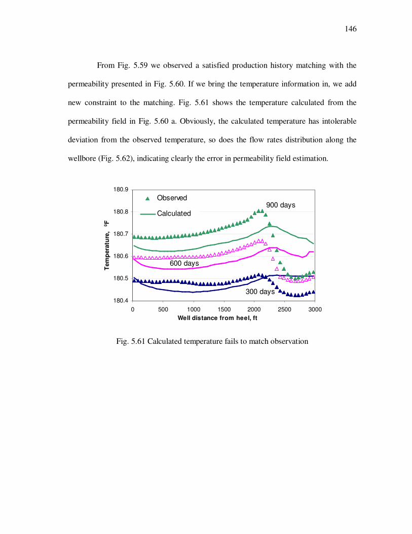
146

From Fig. 5.59 we observed a satisfied production history matching with the

permeability presented in Fig. 5.60. If we bring the temperature information in, we add

new constraint to the matching. Fig. 5.61 shows the temperature calculated from the

permeability field in Fig. 5.60 a. Obviously, the calculated temperature has intolerable

deviation from the observed temperature, so does the flow rates distribution along the

wellbore (Fig. 5.62), indicating clearly the error in permeability field estimation.

180.4

180.5

180.6

180.7

180.8

180.9

0 500 1000 1500 2000 2500 3000

Well distance from heel, ft

Te

mp

era

ture

, 0F

Observed

Calculated 900 days

600 days

300 days

Fig. 5.61 Calculated temperature fails to match observation

147

0

2000

4000

6000

0 500 1000 1500 2000 2500 3000

Well distance from heel, ft

Flo

w r

ate

in

well, b

bl/d

True

Inverted

Water

Oil

Fig. 5.62 Downhole flow rates may not be predicted correctly by history matching only

The procedure of combining the temperature interpretation method and

production history matching has flexibility in generating reservoir characteristics and

horizontal well flow conditions. The results show that the downhole temperature

measurements can improve the understanding of reservoir characteristics. The outcome

is a geologic model that is consistent with the prior static model and dynamic

information, and also the wellbore temperature measurements. The updated model can

then be used to predict the downhole flow conditions in the horizontal well operation.

148

6 CHAPTER VI

CONCLUSIONS

In this study, a methodology has been developed, which can be used to interpret

temperature and pressure data measured by downhole sensors to downhole flow

conditions. The approach uses a forward model to predict the transient temperature, and

pressure based on given flow distribution of horizontal wells, and an inverse model to

estimate the flow profile from temperature and pressure by minimize the objective

function of difference between calculated and observed data. The method has been

applied to examples at field conditions successfully. It is concluded from this study that:

1. The 3D transient flow simulation of reservoir flow and temperature is more

flexible than the previously developed steady-state, 1D model. The simulated

flow field as a function of producing time improves our understanding of

downhole flow condition.

2. The transient flow effect on temperature behavior can provide additional

information of locating of water or gas entries. This information can be used as

preliminary screening of permeability variation along the wellbore.

3. Examples explain the detailed procedure of identifying water entry location and

the effect of reservoir heterogeneity on early water breakthrough by the

developed method. The method located water entry and water flow rate with a

satisfied accuracy.

4. Using temperature feedback to operate ICV to achieve an optimized production

149

is valuable for reservoir/well performance optimization. A desired temperature

profile can be generated by the method introduced in this work, which will yield

an evenly distributed flow profile along a horizontal wellbore, and therefore to

improve downhole flow condition.

5. Finally, temperature data can be extent to reservoir characterization and

optimization. The procedure combines the temperature interpretation method and

production history matching to generate reservoir characteristics and horizontal

well flow conditions. The results show that the integrated downhole temperature

inversion and history matching can improve the understanding of reservoir

characteristics with a better resolution. It clearly demonstrates the benefits of the

approach over either the temperature interpretation only or the production history

matching only.

150

REFERENCES

Alaeddin, E. and Maizeret, P.-D. 2003. Using Production Logging Technology for Reservoir Management in the Persian Gulf. Paper SPE 85667 presented at

Nigeria Annual International Conference and Exhibition, Abuja, Nigeria, 4-6 August. doi: 10.2118/85667-MS.

Alghareeb, Z. M., Horne, R. N., Yuen, B. B. and Shenawi, S. H. 2009. Proactive Optimization of Oil Recovery in Multilateral Wells Using Real Time

Production Data. Paper SPE 124999 presented at SPE Annual Technical Conference and Exhibition, New Orleans, Louisiana, 4-7 October. doi:

10.2118/124999-MS.

Alhuthali, A. H., Oyerinde, D. and Datta-Gupta, A. 2007. Optimal Waterflood

Management Using Rate Control. SPE Reservoir Evaluation & Engineering 10 (5): 539-551. doi: 10.2118/102478-PA.

Behrens, R. A., MacLeod, M. K., Tran, T. T. and Alimi, A. C. 1998. Incorporating Seismic Attribute Maps in 3D Reservoir Models. SPE Reservoir Evaluation &

Engineering 1 (2): 122-126. doi: 10.2118/36499-PA.

Brady, J. L., Watson, B. A., Warner, D. W., North, R. J., Sommer, D. M., Colson, J. L.,

Kleinberg, R. L., Wolcott, D. S. and Sezginer, A. 1998. Improved Production Log Interpretation in Horizontal Wells Using a Combination of Pulsed Neutron

Logs, Quantitative Temperature Log Analysis, Time Lapse LWD Resistivity Logs and Borehole Gravity. Paper SPE 48851 presented at SPE International

Oil and Gas Conference and Exhibition in China, Beijing, China, 2-6 November. doi: 10.2118/48851-MS.

Carnegie, A., Roberts, N. and Clyne, I. 1998. Application of New Generation Technology to Horizontal Well Production Logging - Examples from the North

West Shelf of Australia. Paper SPE 50178 presented at SPE Asia Pacific Oil and Gas Conference and Exhibition, Perth, Australia, 12-14 October 1998. doi:

10.2118/50178-MS.

Chace, D., Wang, J., Mirzwinski, R., Maxit, J. and Trcka, D. 2000. Applications of a

New Multiple Sensor Production Logging System for Horizontal and Highly-Deviated Multiphase Producers. Paper SPE 63141 presented at SPE Annual

Technical Conference and Exhibition, Dallas, Texas, 1-4 October doi: 10.2118/63141-MS.

Chen, N. H. 1979. An Explicit Equation for Friction Factor in Pipe. Ind. Eng. Chem.

Fund. 18 (3): 296.

Cheng, H., Datta-Gupta, A. and He, Z. 2005. A Comparison of Travel-Time and Amplitude Matching for Field-Scale Production-Data Integration: Sensitivity,

151

Nonlinearity, and Practical Implications. SPE Journal 10 (1): 75-90. doi: 10.2118/84570-PA.

Cheng, H., Wen, X.-H., Milliken, W. J. and Datta-Gupta, A. 2004. Field Experiences with Assisted and Automatic History Matching Using Streamline Models.

Paper SPE 89857 presented at SPE Annual Technical Conference and Exhibition, Houston, Texas, 26-29 September. doi: 10.2118/89857-MS.

Datta-Gupta, A. and King, M. J. 2007. Streamline Simulation: Theory and Practice, Textbook Series, SPE, Richardson, Texas 11: 19, 48-51.

Datta-Gupta, A., Kulkarni, K. N., Yoon, S. and Vasco, D. W. 2001. Streamlines, Ray Tracing and Production Tomography: Generalization to Compressible Flow.

Petroleum Geoscience 7 (S): S75-S86.

Deutsch, C. V. and Tran, T. T. 2002. FLUVSIM: A Program for Object-Based

Stochastic Modeling of Fluvial Depositional Systems. Computers &

Geosciences 28 (4): 525-535. doi: 10.1016/S0098-3004(01)00075-9.

Donovan, G., P.E., Dria, D., Ugueto, G. and Gysen, A. 2008. Improved Production Profiling Using Thermal Balance and Statistical Modeling in the Pinedale

Anticline of the US Rocky Mountains. Paper SPE 115034 presented at SPE Annual Technical Conference and Exhibition, Denver, Colorado, 21-24

September. doi:10.2118/115034-MS.

Dranchuk, P. M. and Abou-Kassem. 1975. Calculation of z-Factors for Natural Gases

Using Equations of State. Journal of Canada Petroleum Technology 14 (3): 34-36.

Duru, O. and Horne, R. N. 2008. Modeling Reservoir Temperature Transients and Matching to Permanent Downhole Gauge Data for Reservoir Parameter

Estimation. Paper SPE 115791 presented at SPE Annual Technical Conference and Exhibition, Denver, Colorado, 21-24 September. doi: 10.2118/115791-MS.

Foucault, H., Poilleux, D., Djurisic, A., Slikas, M., Strand, J. and Silva, R. 2004. A Successful Experience for Fiber Optic and Water Shut Off on Horizontal Wells

with Slotted Liner Completion in an Extra Heavy Oil field. Paper SPE 89405 presented at SPE/DOE Symposium on Improved Oil Recovery, Tulsa,

Oklahoma, 17-21 April. doi:10.2118/89405-MS.

Frankenburg, A., Bartel, P., Roberts, G. and Hupp, D. 2000. Gas Shutoff Evaluation and

Implementation, North Slope, Alaska. Paper SPE 62892 presented at SPE Annual Technical Conference and Exhibition, Dallas, Texas, 1-4 October. doi:

10.2118/62892-MS.

FrontSim 2008. S. G. R. T. Reference Manual, 2008.

Fryer, V., ShuXing, D., Otsubo, Y., Brown, G. and Guilfoyle, P. 2005. Monitoring of Real-Time Temperature Profiles Across Multizone Reservoirs during

Production and Shut in Periods Using Permanent Fiber-Optic Distributed

152

Temperature Systems. Paper SPE presented at SPE Asia Pacific Oil and Gas Conference and Exhibition, Jakarta, Indonesia, 5-7 April 2005.

doi:10.2118/92962-MS.

Furui, K., Zhu, D. and Hill, A. D. 2003. A Rigorous Formation Damage Skin Factor and

Reservoir Inflow Model for a Horizontal Well. SPE Production & Facilities 18 (3): 151-157. doi: 10.2118/84964-PA.

Hasan, A. R. and Kabir, C. S. 1994. Aspects of Wellbore Heat Transfer During Two-Phase Flow SPE Production & Facilities 9 (3): 211-216. doi: 10.2118/22948-

PA.

Heddleston, D. 2009. Horizontal Well Production Logging Deployment and

Measurement Techniques for US Land Shale Hydrocarbon Plays. Paper SPE 120591 presented at SPE Production and Operations Symposium, Oklahoma

City, Oklahoma, 4-8 April. 10.2118/120591-MS.

Hill, A. D. 1990. Production Logging -Theoretical and Interpretive Elements,

Monograph Series, SPE, Richardson, Texas 14: 28-29.

Hohl, D., Jimenez, E. and Datta-Gupta, A. 2006. Field Experiences With History

Matching an Offshore Turbiditic Reservoir Using Inverse Modeling. Paper SPE 101983 presented at SPE Annual Technical Conference and Exhibition, San

Antonio, Texas, 24-27 September. doi: 10.2118/101983-MS.

Huckabee, P. 2009. Optic Fiber Distributed Temperature for Fracture Stimulation

Diagnostics and Well Performance Evaluation. Paper SPE presented at SPE Hydraulic Fracturing Technology Conference, The Woodlands, Texas, 19-21

January. doi: 10.2118/118831-MS.

Huebsch, H., Moss, M., Trilsbeck, T., Brown, G., Rogers, S. and Bouchard, T. 2008.

Monitoring Inflow Distribution in Multi-zone, Velocity String Gas Wells Using Slickline Deployed Fiber Optic Distributed Temperature Measurements. Paper

SPE 115816 presented at SPE Annual Technical Conference and Exhibition, Denver, Colorado, USA, 21-24 September doi:10.2118/115816-MS.

Izgec, B., Kabir, C. S., Zhu, D. and Hasan, A. R. 2006. Transient Fluid and Heat Flow Modeling in Coupled Wellbore/Reservoir Systems. SPE Reservoir Evaluation

& Engineering 10 (3): 294-301. doi: 10.2118/102070-PA.

Jayawardena, S. S., Alkaya, B. R. and Brill, C. L. 2000. A New Model for Dispersed

Multi-Layer Oil-Water Flow. BHR Group Conference Series Publication 40: 77-90.

Jerauld, G. R. 1997. General Three-Phase Relative Permeability Model for Prudhoe Bay SPE Reservoir Engineering 12 (4): 255-263. doi: 10.2118/36178-PA.

Johnson, D., Sierra, J., Kaura, J. and Gualtieri, D. 2006. Successful Flow Profiling of Gas Wells Using Distributed Temperature Sensing Data. Paper SPE 103097

153

presented at SPE Annual Technical Conference and Exhibition, San Antonio, Texas, USA, 24-27 September. doi:10.2118/103097-MS.

Johnson, E. F., Bossler, D. P. and Naumann, V. O. 1959. Calculation of Relative Permeability from Displacement Experiments. Petroleum Transactions, AIME

216: 370-372.

Julian, J. Y., King, G. E., Cismoski, D. A., Younger, R. O., Brown, D. L., Brown, G. A.,

Richards, K. M., Meyer, C. A., Sierra, J. R., Leckband, W. T., Sack, J. K. and Julian, F. C. 2007. Downhole Leak Determination Using Fiber-Optic

Distributed-Temperature Surveys at Prudhoe Bay, Alaska. Paper SPE 107070 presented at SPE Annual Technical Conference and Exhibition, Anaheim,

California, 11-14 November doi: 10.2118/107070-MS.

Kabir, C. S., Hasan, A. R., Jordan, D. L. and Wang, X. 1996. A Wellbore/Reservoir

Simulator for Testing Gas Wells in High-Temperature Reservoirs SPE

Formation Evaluation 11 (2): 128-134. doi: 10.2118/28402-PA.

Lake, L. W. 1989. Enhanced Oil Recovery. Englewood Cliffs, New Jersy: Prentice Hall.

Liu, Y. and Journel, A. G. 2009. A package for geostatistical integration of coarse and

fine scale data. Computers & Geosciences 35 (3): 527-547. doi: 10.1016/j.cageo.2007.12.015.

Ma, X., Al-Harbi, M., Datta-Gupta, A. and Efendiev, Y. 2008. An Efficient Two-Stage Sampling Method for Uncertainty Quantification in History Matching

Geological Models. SPE Journal 13 (1): 77-87. doi: 10.2118/102476-PA

Maubeuge, F., Eric, A. and Bertrand, O. 1994. MOTHER: A Model for Interpreting

Thermometrics. Paper SPE 28588 presented at SPE Annual Technical Conference and Exhibition, New Orleans, Louisiana, 25-28 September doi:

10.2118/28588-MS.

Muradov, K. M. and Davies, D. R. 2008. Prediction of Temperature Distribution in

Intelligent Wells. Paper SPE 114772 presented at SPE Russian Oil and Gas Technical Conference and Exhibition, Moscow, Russia, 28-30 October. doi:

10.2118/114772-MS.

Muradov, K. M. and Davies, D. R. 2009. Temperature Modeling and Analysis of Wells

with Advanced Completion. Paper SPE 121054 presented at EUROPEC/EAGE Conference and Exhibition, Amsterdam, The Netherlands, 8-11 June. doi:

10.2118/121054-MS.

Oliver, D. S., Cunha, L. B. and Reynolds, A. C. 1997. Markov chain Monte Carlo

methods for conditioning a permeability field to pressure data. Mathematical

Geology 29 (1): 61-91. doi: 10.1007/BF02769620

Ouyang, L.-B., Arbabi, S. and Aziz, K. 1998. General Wellbore Flow Model for Horizontal, Vertical, and Slanted Well Completions. SPE Journal 3 (2): 124-

133. doi: 10.2118/36608-PA.

154

Ouyang, L.-B. and Aziz, K. 2000. A Homogeneous Model for Gas-Liquid Flow in Horizontal Wells. Journal of Petroleum Science&Engineering 27 (3-4): 119-

128. doi: 10.1016/S0920-4105(00)00053-X.

Ouyang, L.-B. and Belanger, D. 2006. Flow Profiling by Distributed Temperature

Sensor (DTS) System—Expectation and Reality. SPE Production & Operations 21 (2): 269-281. doi: 10.2118/90541-PA.

Paige, C. C. and Saunders, M. A. 1982. An Algorithm for Sparse Linear Equations and Sparse Least Squares. ACM Transactions on Mathematical Software 8 (1): 43-

71. doi: 10.1145/355984.355989.

Peaceman, D. W. 1983. Interpretation of Well-Block Pressures in Numerical Reservoir

Simulation With Nonsquare Grid Blocks and Anisotropic Permeability. SPE

Journal 23 (3): 531-543. doi: 10.2118/10528-PA.

Perkins, T. K. 1993. Critical and Subcritical Flow of Multiphase Mixtures Through Chokes. SPE Drilling & Completion 8 (4): 271-276. doi: 10.2118/20633-PA

Pinzon, I. D., Davies, J. E., Mammadkhan, F. and Brown, G. A. 2007. Monitoring Production From Gravel-Packed Sand-Screen Completions on BP’s Azeri Field

Wells Using Permanently Installed Distributed Temperature Sensors. Paper SPE 110064 presented at SPE Annual Technical Conference and Exhibition,

Anaheim, California, USA, 11-14 November. doi:10.2118/110064-MS.

Pollock, D. W. 1988. Semeanalytical Computation of Path Lines for Finite-Difference

Models. Ground Water 26 (6): 743-750.

Qing, Y. and Davies, D. R. 2009. A Generalized Predictive Control for Management of

an Intelligent Well’s Downhole, Interval Control Valves—Design and Practical Implementation. Paper SPE 123682 presented at Offshore Europe, Aberdeen,

UK, 8-11 September. doi: 10.2118/123682-MS.

Ramey, H. J. 1962. Wellbore Heat Transmission. Journal of Petroleum Technology 14

(4): 427-435. doi: 10.2118/96-PA.

Rey, A., Ballin, P. R., Vitalis, C. F., Parke, J. and Datta-Gupta, A. 2009. Assisted

History Matching in an Offshore Turbidite Reservoir With Active Reservoir Management. Paper SPE 124950 presented at SPE Annual Technical

Conference and Exhibition, New Orleans, Louisiana, 4-7 October. doi: 10.2118/124950-MS.

Sagar, R., Doty, D. R. and Schmidt, Z. 1991. Predicting Temperature Profiles in a Flowing Well SPE Production Engineering 6 (4): 441-448. doi:

10.2118/19702-PA.

Satter, A. 1965. Heat Losses During Flow of Steam Down a Wellbore. Journal of

Petroleum Technology 17 (7): 845-851. doi: 10.2118/1071-PA.

155

Sui, W. 2009. Determining Multilayer Formation Properties from Transient Temperature and Pressure Measurements. PhD thesis, Texas A&M Univeristy, College

Station, Texas.

Sui, W., Zhu, D., Hill, A. D. and Ehlig-Economides, C. A. 2008a. Determining

Multilayer Formation Properties From Transient Temperature and Pressure Measurements. Paper SPE 116270 presented at SPE Annual Technical

Conference and Exhibition, Denver, Colorado, USA, 21-24 September. doi:10.2118/116270-MS.

Sui, W., Zhu, D., Hill, A. D. and Ehlig-Economides, C. A. 2008b. Model for Transient Temperature and Pressure Behavior in Commingled Vertical Wells. Paper SPE

115200 presented at SPE Russian Oil and Gas Technical Conference and Exhibition, Moscow, Russia, 28-30 October. doi:10.2118/115200-MS.

Wang, X., Lee, J., Thigpen, B., Vachon, G., Poland, S. and Norton, D. 2008. Modeling Flow Profile Using Distributed Temperature Sensor (DTS) System. Paper SPE

presented at Intelligent Energy Conference and Exhibition, Amsterdam, The Netherlands, 25-27 February doi: 10.2118/111790-MS.

Willhite, G. P. 1967. Over-all Heat Transfer Coefficients in Steam And Hot Water Injection Wells. Journal of Petroleum Technology 19 (5): 607-615. doi:

10.2118/1449-PA.

Yoshioka, K. 2007. Detection of Water or Gas Entry into Horizontal Wells by Using

Permanent Downhole Monitoring System. PhD thesis, Texas A&M Univeristy, College Station, Texas.

Yoshioka, K., Zhu, D. and Hill, A. D. 2007a. A New Inversion Method to Interpret Flow Profiles From Distributed Temperature and Pressure Measurements in

Horizontal Wells. Paper SPE 109749 presented at SPE Annual Technical Conference and Exhibition, Anaheim, California, 11-14 November.

doi:10.2118/109749-MS.

Yoshioka, K., Zhu, D., Hill, A. D., Dawkrajai, P. and Lake, L. W. 2007b. Prediction of

Temperature Changes Caused by Water or Gas Entry Into a Horizontal Well. SPE Production & Operations 22 (4): 425-433. doi: 10.2118/100209-PA.

Yoshioka, K., Zhu, D., Hill, A. D., Dawkrajai, P. and Lake, L. W. 2005. A Comprehensive Model of Temperature Behavior in a Horizontal Well. Paper

SPE 95656 presented at SPE Annual Technical Conference and Exhibition, Dallas, Texas, 9-12 October. doi:10.2118/95656-MS.

156

APPENDIX A

DIFFERENTIAL SCHEME OF RESERVOIR TEMPERATURE EQUATION

The partial difference equation for reservoir temperature has already been derived from

reservoir energy balance as follows:

( ) ( )

( )

( ) ( )∑∑

∑∑

∑∑

∇⋅+∇⋅−

∇⋅+∇⋅∇−∇⋅=

∂

∂+

∂

∂

−+−

l

ll

l

lll

l

llTt

l

plll

l

lllpss

l

plll

gDupuT

puTKTCu

t

pTS

t

TCCS

vv

vv

ρβ

ρ

βφρφρφ 1

................................ (A-1)

This appendix provides the differential procedure of this equation by Finite Volume

Scheme (FVS) method. To avoid the general meaning of i as x direction grid, the

subscript l is used to represent the fluid phase, it could be oil, gas, or water.

First, substituting the mass balance equation of each phase

( ) ( )llll St

u φρρ∂

∂−=⋅∇

v............................................................................. (A-2)

into Eq. A-1. Then Eq. A-1 becomes:

( ) ( )

( ) ( )

( ) ( )∑∑

∑∑

∑∑

∇⋅+∇⋅−

∇⋅+∇⋅∇−∇=

∂

∂+

∂

∂−+

∂

∂−

l

ll

l

lll

l

llTt

l

llpl

l

lllpss

ll

l

pi

gDupuT

puTKTuC

t

pTS

t

TC

t

TSC

vv

vv

ρβ

ρ

βφρφρφ

1

......................... (A-3)

For the black oil, three Phase case, Eq. A-3 can be written as

157

( ) ( ) ( )( )

( ) ( ) ( )[ ] ( )

( )( ) ( )gDuuupupupu

Tpupupu

TKTuCTuCTuC

Tt

pS

t

pS

t

pS

t

TC

t

TSC

t

TSC

t

TSC

ggwwooggwwoo

gggwwwooo

Ttggpgwwpwoopo

g

ggw

wwo

oo

pss

gg

pgww

pwoo

po

∇⋅+++∇⋅+∇⋅+∇⋅+

∇⋅+∇⋅+∇⋅−

∇⋅∇−⋅∇+⋅∇+⋅∇=

∂

∂+

∂

∂+

∂

∂+

∂

∂−+

∂

∂+

∂

∂+

∂

∂−

vvvvvv

vvv

vvv

ρρρ

βββ

ρρρ

βββφ

ρφρφρφρφ

1

... (A-4)

RHS Expression of FVS Method

The expansion form for RHS of Eq. A-4 can be written down as:

( ) ( ) ( )( ) ( ) ( )

( ) ( ) ( )

( ) ( ) ( )

∂

∂+

∂

∂+

∂

∂+

∂

∂+

∂

∂+

∂

∂+

∂

∂+

∂

∂+

∂

∂

=⋅∇+⋅∇+⋅∇

z

Tu

y

Tu

x

TuC

z

Tu

y

Tu

x

TuC

z

Tu

y

Tu

x

TuC

TuCTuCTuC

gzggyggxg

pg

wzwwywwxwpw

ozooyooxopo

ggpgwwpwoopo

ρρρ

ρρρ

ρρρ

ρρρvvv

............................... (A-5)

( )

∂

∂

∂

∂+

∂

∂

∂

∂+

∂

∂

∂

∂=∇⋅∇

y

TK

yy

TK

yx

TK

xTK TtTtTtTt ........................... (A-6)

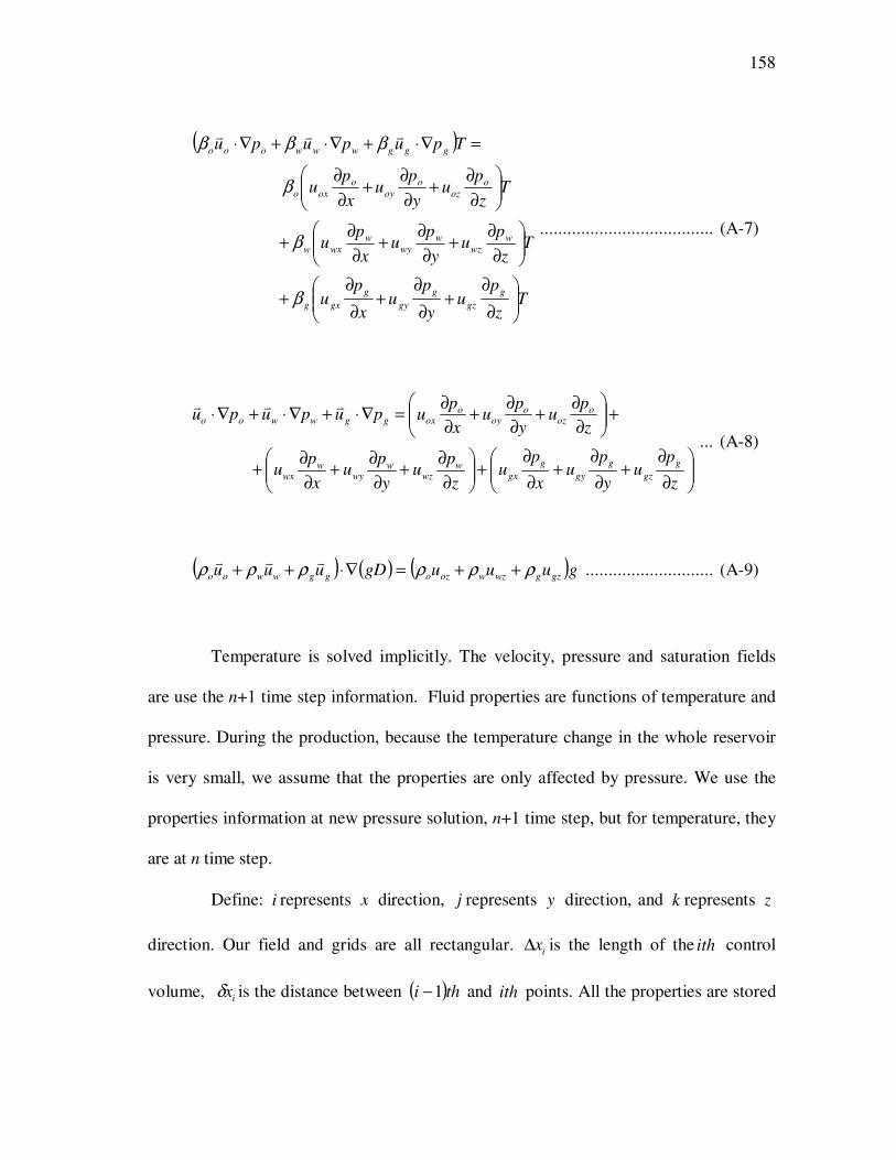
158

( )

Tz

pu

y

pu

x

pu

Tz

pu

y

pu

x

pu

Tz

pu

y

pu

x

pu

Tpupupu

g

gz

g

gy

g

gxg

w

wz

w

wy

w

wxw

o

oz

o

oy

o

oxo

gggwwwooo

∂

∂+

∂

∂+

∂

∂+

∂

∂+

∂

∂+

∂

∂+

∂

∂+

∂

∂+

∂

∂

=∇⋅+∇⋅+∇⋅

β

β

β

βββvvv

...................................... (A-7)

∂

∂+

∂

∂+

∂

∂+

∂

∂+

∂

∂+

∂

∂+

+

∂

∂+

∂

∂+

∂

∂=∇⋅+∇⋅+∇⋅

z

pu

y

pu

x

pu

z

pu

y

pu

x

pu

z

pu

y

pu

x

pupupupu

g

gz

g

gy

g

gxw

wzw

wyw

wx

ooz

ooy

ooxggwwoo

vvv

... (A-8)

( ) ( ) ( )guuugDuuu gzgwzwozoggwwoo ρρρρρρ ++=∇⋅++vvv

............................ (A-9)

Temperature is solved implicitly. The velocity, pressure and saturation fields

are use the n+1 time step information. Fluid properties are functions of temperature and

pressure. During the production, because the temperature change in the whole reservoir

is very small, we assume that the properties are only affected by pressure. We use the

properties information at new pressure solution, n+1 time step, but for temperature, they

are at n time step.

Define: i represents x direction, j represents y direction, and k represents z

direction. Our field and grids are all rectangular. ix∆ is the length of the ith control

volume, ixδ is the distance between ( )thi 1− and ith points. All the properties are stored

159

on the points. All the velocities are stored at the interface of grids. The velocity from

Darcy’s law:

( )( ) ( )

i

ilil

rlxilxx

gDpgDpku

δ

ρρλ 1

2/1

−−

−−−−= ............................................ (A-10)

whereµ

λ rr

k= , and l could be oil, water, or gas. k is absolutely permeability, rk is

relative permeability. And we use upwind scheme for velocity calculation.

Now we apply finite volume scheme to Eq. A-4. For the convection term in

temperature, Eq. A-5 has three terms about different fluid phases. Here we just give oil

phase term as example (all other terms are the same):

( ) ( ) ( )

( ) ( ) ( ) ( ) ( )[ ]( ) ( ) ( ) ( ) ( )[ ]( ) ( ) ( ) ( ) ( )[ ] tyxTuTuC

tzxTuTuC

tzyTuTuC

dxdydzdtz

Tu

y

Tu

x

TuC

ji

n

kji

n

kjioz

n

kjio

n

kji

n

kjioz

n

kjio

n

kjipo

ki

n

kji

n

kjioy

n

kjio

n

kji

n

kjioy

n

kjio

n

kjipo

kj

n

kji

n

kjiox

n

kjio

n

kji

n

kjiox

n

kjio

n

kjipo

ozooyooxopo

z

z

y

y

x

x

t

t

k

k

j

j

i

i

n

n

∆∆∆−+

∆∆∆−+

∆∆∆−=

∂

∂+

∂

∂+

∂

∂

+−

+

−

+

−

++

+

+

+

+

+

+−

+

−

+

−

++

+

+

+

+

+

+−

+

−

+

−

++

+

+

+

+

+

∫∫∫∫+

−

+

−

+

−

+

1

2/1,,

1

2/1,,

1

2/1,,

1

2/1,,

1

2/1,,

1

2/1,,

1

,,

1

,2/1,

1

,2/1,

1

,2/1,

1

,2/1,

1

,2/1,

1

,2/1,

1

,,

1

,,2/1

1

,,2/1

1

,,2/1

1

,,2/1

1

,,2/1

1

,,2/1

1

,,

2/1

2/1

2/1

2/1

2/1

2/1

1

ρρ

ρρ

ρρ

ρρρ

........................................................................................................................ (A-11)

Use upstream scheme for the “1/2” term, which means:

If ( ) 0,,2/1

>− kjioxu , 1

,,1

1

,,2/1

+−

+− = n

kji

n

kji TT ............................................................. (A-12)

For the thermal conduction term in reservoir, Eq. A-6 can be expressed as:

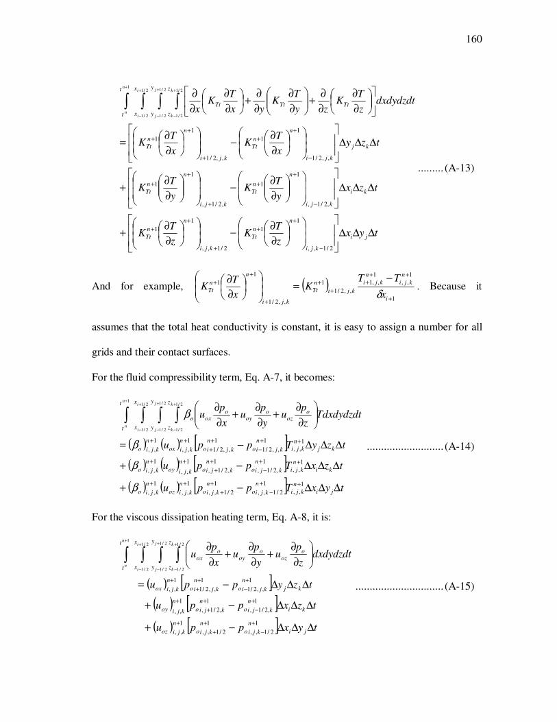
160

tyxz

TK

z

TK

tzxy

TK

y

TK

tzyx

TK

x

TK

dxdydzdtz

TK

zy

TK

yx

TK

x

ji

kji

n

n

Tt

kji

n

n

Tt

ki

kji

n

n

Tt

kji

n

n

Tt

kj

kji

n

n

Tt

kji

n

n

Tt

TtTtTt

z

z

y

y

x

x

t

t

k

k

j

j

i

i

n

n

∆∆∆

∂

∂−

∂

∂+

∆∆∆

∂

∂−

∂

∂+

∆∆∆

∂

∂−

∂

∂=

∂

∂

∂

∂+

∂

∂

∂

∂+

∂

∂

∂

∂

−

+

+

+

+

+

−

+

+

+

+

+

−

+

+

+

+

+

∫∫∫∫+

−

+

−

+

−

+

2/1,,

1

1

2/1,,

1

1

,2/1,

1

1

,2/1,

1

1

,,2/1

1

1

,,2/1

1

1

2/1

2/1

2/1

2/1

2/1

2/1

1

......... (A-13)

And for example, ( )1

1

,,

1

,,1

,,2/1

1

,,2/1

1

1

+

+++

+

+

+

+

+ −=

∂

∂

i

n

kji

n

kji

kji

n

Tt

kji

n

n

Ttx

TTK

x

TK

δ. Because it

assumes that the total heat conductivity is constant, it is easy to assign a number for all

grids and their contact surfaces.

For the fluid compressibility term, Eq. A-7, it becomes:

( ) ( ) [ ]( ) ( ) [ ]( ) ( ) [ ] tyxTppu

tzxTppu

tzyTppu

Tdxdydzdtz

pu

y

pu

x

pu

ji

n

kji

n

kjio

n

kjio

n

kjioz

n

kjio

ki

n

kji

n

kjio

n

kjio

n

kjioy

n

kjio

kj

n

kji

n

kjio

n

kjio

n

kjiox

n

kjio

ooz

ooy

ooxo

z

z

y

y

x

x

t

t

k

k

j

j

i

i

n

n

∆∆∆−+

∆∆∆−+

∆∆∆−=

∂

∂+

∂

∂+

∂

∂

++

−

+

+

++

++

−

+

+

++

++

−

+

+

++

∫∫∫∫+

−

+

−

+

−

+

1

,,

1

2/1,,

1

2/1,,

1

,,

1

,,

1

,,

1

,2/1,

1

,2/1,

1

,,

1

,,

1

,,

1

,,2/1

1

,,2/1

1

,,

1

,,

2/1

2/1

2/1

2/1

2/1

2/1

1

β

β

β

β

........................... (A-14)

For the viscous dissipation heating term, Eq. A-8, it is:

( ) [ ]( ) [ ]( ) [ ] tyxppu

tzxppu

tzyppu

dxdydzdtz

pu

y

pu

x

pu

ji

n

kjio

n

kjio

n

kjioz

ki

n

kjio

n

kjio

n

kjioy

kj

n

kjio

n

kjio

n

kjiox

ooz

ooy

oox

z

z

y

y

x

x

t

t

k

k

j

j

i

i

n

n

∆∆∆−+

∆∆∆−+

∆∆∆−=

∂

∂+

∂

∂+

∂

∂

+

−

+

+

+

+

−

+

+

+

+

−

+

+

+

∫∫∫∫+

−

+

−

+

−

+

1

2/1,,

1

2/1,,

1

,,

1

,2/1,

1

,2/1,

1

,,

1

,,2/1

1

,,2/1

1

,,

2/1

2/1

2/1

2/1

2/1

2/1

1

............................... (A-15)

161

For the potential energy term, Eq. A-9 has the following form:

( )

( ) tzyxguuu

gdxdydzdtuuu

kji

n

kjigzgwzwozo

gzgwzwozo

z

z

y

y

x

x

t

t

k

k

j

j

i

i

n

n

∆∆∆∆++=

++

+

∫∫∫∫+

−

+

−

+

−

+

1

,,

2/1

2/1

2/1

2/1

2/1

2/1

1

ρρρ

ρρρ............................... (A-16)

LHS Expression of FVS Method

The LHS of Eq. A-5 includes the accumulative term and the thermal expansion term

relative to transient pressure change. For the accumulative term, it is:

( ) ( ) ( )( )

( ) ( )( ) ( ) ( )( )( ) ( )( )

( )( ) ( )

( ) ( ) ( ) ( )( )( )[( ) ( ) ( ) ( )( )( ) ]

kji

n

kjikji

n

pss

n

gg

n

pg

n

ww

n

pw

n

oo

n

po

n

kjikji

n

pss

n

gg

n

pg

n

ww

n

pw

n

oo

n

po

kji

n

kji

n

kji

n

kjipss

kji

kji

n

gg

n

gg

n

pg

n

ww

n

ww

n

pw

n

oo

n

oo

n

po

z

z

pss

ggpgwwpwoopo

y

y

x

x

t

t

zyxTCSCSCSC

TCSCSCSC

zyxTTC

zyxTSTSC

TSTSCTSTSC

dxdydzdtt

TC

t

TSC

t

TSC

t

TSCk

k

j

j

i

i

n

n

∆∆∆−+++−

−+++=

∆∆∆−−+

∆∆∆

−+

−+−=

∂

∂−+

∂

∂+

∂

∂+

∂

∂

++++

++++++++

++

++

++++

∫∫∫∫+

−

+

−

+

−

+

,,,,

1111

1

,,,,

1111111

,,

1

,,

1

,,

,,

11

1111

1

1

1

12/1

2/1

2/1

2/1

2/1

2/1

1

ρφρφρφρφ

ρφρφρφρφ

ρφ

ρφρφ

ρφρφρφρφ

ρφρφρφρφ

........................................................................................................................... (A-17)

For the thermal expansion term, the formulation becomes:

( )( ) ( ) ( )( ) ( )[( )( ) ( )] kji

n

kji

n

kjig

n

kjig

n

kjigg

n

kjiw

n

kjiw

n

kjiww

n

kjio

n

kjio

n

kjioo

g

ggw

wwo

oo

z

z

y

y

x

x

t

t

zyxTppS

ppSppS

Tdxdydzdtt

pS

t

pS

t

pS

k

k

j

j

i

i

n

n

∆∆∆⋅−+

−+−=

∂

∂+

∂

∂+

∂

∂

+++

++++

∫∫∫∫+

−

+

−

+

−

+

1

,,,,

1

,,

1

,,

,,

1

,,

1

,,,,

1

,,

1

,,

2/1

2/1

2/1

2/1

2/1

2/1

1

βφ

βφβφ

βββφ

................... (A-18)

162

General Expression for Discretized Equation

Substituting Eq. A-11 through Eq. A-18 into Eq. 4, and rearranging it, the general

discretized equation is given by:

kji

n

kjikji

n

kjikji

n

kjikji

n

kjikji

n

kjikji

n

kjikji

n

kjikji

BTATTAB

TANTASTAETAWTAP

,,

1

1,,,,

1

1,,,,

1

,1,,,

1

,1,,,

1

,,1,,

1

,,1,,

1

,,,,

+++

+++=

++

+−

++

+−

++

+−

+

...... (A-19)

First, declare [ ] ( )0,max0, aa = ; Then

( )( ) ( )[ ]

( ) ( )[ ]( ) ( )[ ]) tzyuC

uC

uCx

KAW

kj

n

kjigxg

n

kjipg

n

kjiwxw

n

kjipw

n

kjioxo

n

kjipo

i

kji

n

Tt

kji

∆∆∆+

+

+=

+

−

+

+

−

+

+

−

+−

+

0,

0,

0,

1

,,2/1

1

,,

1

,,2/1

1

,,

1

,,2/1

1

,,

,,2/1

1

,,

ρ

ρ

ρδ

............................... (A-20)

( )( ) ( )[ ]

( ) ( )[ ]( ) ( )[ ]) tzyuC

uC

uCx

KAE

kj

n

kjigxg

n

kjipg

n

kjiwxw

n

kjipw

n

kjioxo

n

kjipo

i

kji

n

Tt

kji

∆∆∆−+

−+

−+=

+

+

+

+

+

+

+

+

+

+

+

+

0,

0,

0,

1

,,2/1

1

,,

1

,,2/1

1

,,

1

,,2/1

1

,,1

,,2/1

1

,,

ρ

ρ

ρδ

............................. (A-21)

( )( ) ( )[ ]

( ) ( )[ ]( ) ( )[ ]) tzxuC

uC

uCy

KAS

ki

n

kjigyg

n

kjipg

n

kjiwyw

n

kjipw

n

kjioyo

n

kjipo

j

kji

n

Tt

kji

∆∆∆+

+

+=

+

−

+

+

−

+

+

−

+−

+

0,

0,

0,

1

,2/1,

1

,,

1

,2/1,

1

,,

1

,2/1,

1

,,

,2/1,

1

,,

ρ

ρ

ρδ

................................ (A-22)

163

( )( ) ( )[ ]

( ) ( )[ ]( ) ( )[ ]) tzxuC

uC

uCy

KAN

ki

n

kjigyg

n

kjipg

n

kjiwyw

n

kjipw

n

kjioyo

n

kjipo

j

kji

n

Tt

kji

∆∆∆−+

−+

−+=

+

+

+

+

+

+

+

+

+

+

+

+

0,

0,

0,

1

,2/1,

1

,,

1

,2/1,

1

,,

1

,2/1,

1

,,1

,2/1,

1

,,

ρ

ρ

ρδ

............................. (A-23)

( )( ) ( )[ ]

( ) ( )[ ]( ) ( )[ ]) tyxuC

uC

uCz

KAB

ji

n

kjigzg

n

kjipg

n

kjiwzw

n

kjipw

n

kjiozo

n

kjipo

k

kji

n

Tt

kji

∆∆∆+

+

+=

+

−

+

+

−

+

+

−

+−

+

0,

0,

0,

1

2/1,,

1

,,

1

2/1,,

1

,,

1

2/1,,

1

,,

2/1,,

1

,,

ρ

ρ

ρδ

................................ (A-24)

( )( ) ( )[ ]

( ) ( )[ ]( ) ( )[ ]) tyxuC

uC

uCz

KAT

ji

n

kjigzg

n

kjipg

n

kjiwzw

n

kjipw

n

kjiozo

n

kjipo

k

kji

n

Tt

kji

∆∆∆−+

−+

−+=

+

+

+

+

+

+

+

+

+

+

+

+

0,

0,

0,

1

2/1,,

1

,,

1

2/1,,

1

,,

1

2/1,,

1

,,1

2/1,,

1

,,

ρ

ρ

ρδ

............................. (A-25)

and

kjikjikjikjikji APAPAPAPAP,,4,,3,,2,,1,, +++= .............................................. (A-26)

where:

kjiAP

,,1 : The coefficients from conductivity and convection terms.

kjiAP

,,2 : The coefficients from the nondeterministic term, time-dependent term.

kjiAP

,,3 : The coefficients from the space pressure compressible term.

kjiAP

,,4 : The coefficients from the time pressure compressible term.

164

The detailed expressions of these four components are written as follows:

( ) ( )( ) ( )[ ]

( ) ( )[ ]

( ) ( )( ) ( )[ ]

( ) ( )[ ]( ) ( )

( ) ( )[ ]

( ) ( )[ ]tyx

uC

uCz

K

z

K

tzx

uC

uCy

K

y

K

tzy

uC

uCx

K

x

K

AP

ji

l

n

kjilzl

n

kjipl

l

n

kjilzl

n

kjipl

k

kji

n

Tt

k

kji

n

Tt

ki

l

n

kjilyl

n

kjipl

l

n

kjilyl

n

kjipl

j

kji

n

Tt

j

kji

n

Tt

kj

l

n

kjilxl

n

kjipl

l

n

kjilxl

n

kjipl

i

kji

n

Tt

i

kji

n

Tt

kji

∆∆∆

−

+++

+

∆∆∆

−

+++

+

∆∆∆

−

+++

=

∑

∑

∑

∑

∑

∑

=

+

−

+

=

+

+

+

+

+

+

−

+

=

+

−

+

=

+

+

+

+

+

+

−

+

=

+

−

+

=

+

+

+

+

+

+

−

+

3

1

1

2/1,,

1

,,

3

1

1

2/1,,

1

,,1

,,2/1

1

2/1,,

1

3

1

1

,2/1,

1

,,

3

1

1

,2/1,

1

,,1

,2/1,

1

,2/1,

1

3

1

1

,,2/1

1

,,

3

1

1

,,2/1

1

,,1

,,2/1

1

,,2/1

1

,,1

0,

0,

0,

0,

0,

0,

ρ

ρδδ

ρ

ρδδ

ρ

ρδδ

........................................................................................................................... (A-27)

( ) ( )(( ) ( )( ) )

kjikji

n

pss

n

gg

n

pg

n

ww

n

pw

n

oo

n

pokji

zyxCSC

SCSCAP

∆∆∆−++

+=

+++

++++

,,

111

1111

,,2

1 ρφρφ

ρφρφ................... (A-28)

( ) [ ]( ) [ ]( ) [ ]( ) [ ]( ) [ ]( ) [ ]( ) [ ]( ) [ ]( ) [ ] tyxppu

tzxppu

tzyppu

tyxppu

tzxppu

tzyppu

tyxppu

tzxppu

tzyppuAP

ji

n

kjig

n

kjig

n

kjigzg

ki

n

kjig

n

kjig

n

kjigyg

kj

n

kjig

n

kjig

n

kjigxg

ji

n

kjiw

n

kjiw

n

kjiwzw

ki

n

kjiw

n

kjiw

n

kjiwyw

kj

n

kjiw

n

kjiw

n

kjiwxw

ji

n

kjio

n

kjio

n

kjiozo

ki

n

kjio

n

kjio

n

kjioyo

kj

n

kjio

n

kjio

n

kjioxokji

∆∆∆−+

∆∆∆−+

∆∆∆−+

∆∆∆−+

∆∆∆−+

∆∆∆−+

∆∆∆−+

∆∆∆−+

∆∆∆−=−

+

−

+

+

+

+

−

+

+

+

+

−

+

+

+

+

−

+

+

+

+

−

+

+

+

+

−

+

+

+

+

−

+

+

+

+

−

+

+

+

+

−

+

+

+

1

2/1,,

1

2/1,,

1

,,

1

,2/1,

1

,2/1,

1

,,

1

,,2/1

1

,,2/1

1

,,

1

2/1,,

1

2/1,,

1

,,

1

,2/1,

1

,2/1,

1

,,

1

,,2/1

1

,,2/1

1

,,

1

2/1,,

1

2/1,,

1

,,

1

,2/1,

1

,2/1,

1

,,

1

,,2/1

1

,,2/1

1

,,,,3

β

β

β

β

β

β

β

β

β

................................. (A-29)

165

( )( ) ( ) ( )( ) ( )[( )( ) ( )] kji

n

kjig

n

kjig

n

kjigg

n

kjiw

n

kjiw

n

kjiww

n

kjio

n

kjio

n

kjiookji

zyxppS

ppSppSAP

∆∆∆⋅−+

−+−−=

++

++++

,,

1

,,

1

,,

,,

1

,,

1

,,,,

1

,,

1

,,,,4

βφ

βφβφ...... (A-30)

From the mass balance, Eq. A-2, we can find that

( ) ( ) ( )( )( )( )

kjikjikjikjikjikjikji

kji

n

kjipss

kjikji

n

gg

n

pg

n

ww

n

pw

n

oo

n

po

kjikjikjikjikjikjikjikji

PAATABANASAEAW

zyxC

zyxSCSCSC

ATABANASAEAWAPAP

,,2,,,,,,,,,,,,

1

,,

,,

,,,,,,,,,,,,,,2,,1

1

′++++++=

∆∆∆−+

∆∆∆+++

+++++=+

+ρφ

ρφρφρφ......... (A-31)

where

( ) ( ) ( )( )( )( )

kji

n

kjipss

kjikji

n

gg

n

pg

n

ww

n

pw

n

oo

n

pokji

zyxC

zyxSCSCSCPA

∆∆∆−+

∆∆∆++=′

+1

,,

,,,,2

1 ρφ

ρφρφρφ............... (A-32)

Therefore,

kjikjikji

kjikjikjikjikjikjikji

APAPPA

ATABANASAEAWAP

,,4,,3,,2

,,,,,,,,,,,,,,

++′+

+++++=..................... (A-33)

With Eq. A-31, there is another way to calculatekji

AP,,1 , and

kjiAP

,,2 is replaced

bykji

PA,,2

′ .

For the source term, kjiB ,, , its formulation is:

kjikjikjikji BBBB,,3,,2,,1,, ++= ...................................................................... (A-34)

where

kjiB

,,1 : From Eq. A-15, the viscous dissipation heating term.

kjiB

,,2 : From Eq. A-16, the potential energy, gravity term.

166

kjiB

,,3 : From previous time step temperature, n

kjiT ,,

The detailed expressions are:

( ) ( )( ) ( )

( ) ( ) ( ) ( )( ) ( ) ( ) ( )( ) ( ) ( ) ( )( ) ( ) tyxppu

tzxpputzyppu

tyxpputzxppu

tzypputyxppu

tzxppu

tzyppuB

ji

n

kjig

n

kjig

n

kjigz

ki

n

kjig

n

kjig

n

kjigykj

n

kjig

n

kjig

n

kjigx

ji

n

kjiw

n

kjiw

n

kjiwzki

n

kjiw

n

kjiw

n

kjiwy

kj

n

kjiw

n

kjiw

n

kjiwxji

n

kjio

n

kjio

n

kjioz

ki

n

kjio

n

kjio

n

kjioy

kj

n

kjio

n

kjio

n

kjioxkji

∆∆∆−+

∆∆∆−+∆∆∆−+

∆∆∆−+∆∆∆−+

∆∆∆−+∆∆∆−+

∆∆∆−+

∆∆∆−=−

+

−

+

+

+

+

−

+

+

++

−

+

+

+

+

−

+

+

++

−

+

+

+

+

−

+

+

++

−

+

+

+

+

−

+

+

+

+

−

+

+

+

1

2/1,,

1

2/1,,

1

,,

1

,2/1,

1

,2/1,

1

,,

1

,,2/1

1

,,2/1

1

,,

1

2/1,,

1

2/1,,

1

,,

1

,2/1,

1

,2/1,

1

,,

1

,,2/1

1

,,2/1

1

,,

1

2/1,,

1

2/1,,

1

,,

1

,2/1,

1

,2/1,

1

,,

1

,,2/1

1

,,2/1

1

,,,,1

........................................................................................................................... (A-35)

( ) tzyxguuuB kji

n

kjigzgwzwozokji∆∆∆∆++−=

+1

,,,,2 ρρρ .................................... (A-36)

( ) ( ) ( )(( )( ) ) kji

n

kjikji

n

pss

n

gg

n

pg

n

ww

n

pw

n

oo

n

pokji

zyxTC

SCSCSCB

∆∆∆−+

++=

+

+++

,,,,

1

111

,,3

1 ρφ

ρφρφρφ................................ (A-37)

The Variance Value at Grid Surface

As mentioned before, all the properties are stored on the points. All the velocities are

stored at the interface of grids.

For pressure, use arithmetic average, which means pressure is linear change between too

grid centers.

( ) ( )iiikjilikjilkjil xxxpxpp ∆+∆∆⋅+∆⋅= −−−− 1,,1,,1,,2/1/

( ) ( )jjjkjiljkjilkjil yyypypp ∆+∆∆⋅+∆⋅= −−−− 1,,1,1,,2/1,/

( ) ( )kkkkjilkkjilkjil zzzpzpp ∆+∆∆⋅+∆⋅= −−−− 1,,11,,2/1,,/

167

For velocity, ( ) ( )( ) ( )

i

ilil

kjirlxkjilxx

ppku

δλ 1

,,2/1,,2/1

−−−

−−= , where xk is the absolute

permeability, µ

λ rr

k= , rk is the relative permeability, µ is the viscosity.

Harmonic average for xk

1

,,,,1

1,,2/1

2/2/−

−

−−

∆+

∆=

kjix

i

kjix

iikjix

k

x

k

xxk δ , where ( ) 2/1 iii xxx ∆+∆= −δ

Upstream scheme for relative permeability rk

If ( ) ( )ilil pp ≥

−1,

kjirkjir kk,,1,,2/1 −−

= , elsekjirkjir kk

,,,,2/1=

−

Arithmetic average for viscosity µ

( ) ( )iiikjilikjilkjil xxxx ∆+∆∆⋅+∆⋅= −−−− 1,,1,,1,,2/1/µµµ

And the velocity on the point, because the ½ is at the grid surface (edge), so for these

velocities: kjiou

,,,

kjiwu,, kjigu

,,

( ) 2/,,2/1,,2/1,, kjilxkjilxkjilx uuu

+−+= ,

( ) 2/,2/1,,2/1,,, kjilykjilykjily uuu

+−+= ,

( ) 2/2/1,,2/1,,,, +−

+=kjilzkjilzkjilz uuu

For heat conductivity TtK , use harmonic average

( ) ( ) ( )kjiTt

i

kjiTt

i

kjiTt

i

K

x

K

x

K

x

,,,,1

1

,,2/1

2/2/ ∆+

∆=

−

−

−

δ, for rectangular grids: ( ) 2/1 iii xxx ∆+∆= −δ

168

So ( )( ) ( )

1

,,,,1

1,,2/1

2/2/−

−

−−

∆+

∆=

kjiTt

i

kjiTt

iikjiTt

K

x

K

xxK δ

and ( )( ) ( )

1

,,1

1

,,

1,,2/1

2/2/−

+

+++

∆+

∆=

kjiTt

i

kjiTt

iikjiTt

K

x

K

xxK δ

For each phase density, oρ , wρ , gρ , use arithmetic average:

( ) ( )iiikjilikjilkjil xxxx ∆+∆∆⋅+∆⋅= −−−− 1,,1,,1,,2/1/ρρρ , l=1, 2, 3, which can represent oil,

water, and gas.

Now, with all equations above, we obtain a large linear matrix of temperature

equations:

BTA = ................................................................................................... (A-38)

where A is the coefficients matrix, which is a large sparse matrix, T is the unknown

temperature vector, and B is the source term.

The coefficients matrix A has seven linear domains which include non-zero

elements, and all other elements in matrix A are zero.

169

=

****

*****

*****

*****

**

***

*****

*****

*****

***

**

*****

*****

*****

****

A

Then, a program can be developed to solve this set of equations and obtain temperature

behavior in reservoir.

170

VITA

Name: Zhuoyi Li

Contact: c/o Dr. Ding Zhu

Department of Petroleum Engineering

Texas A&M University

College Station, TX 77843-3116

Email Address: lizhuoyi99@gmail.com

Education: B.E., Engineering Mechanics, Tsinghua University, 2003

M.E., School of Aerospace, Tsinghua University. 2005

Ph. D, Petroleum Engineering, Texas A&M University, 2010