interstellar turbulent velocity fields: scaling properties, synthesis and

A&A 389, 1055–1067 (2002)DOI: 10.1051/0004-6361:20020613c© ESO 2002

Astronomy&

Astrophysics

Interstellar turbulent velocity fields: Scaling properties, synthesisand effects on chemistry?

N. Decamp and J. Le Bourlot

LUTH, Observatoire de Paris et Universite Paris 7, France

Received 26 November 2001 / Accepted 3 April 2002

Abstract. Turbulence is thought to play a key role in the dynamics of interstellar clouds. Here, we do not seek toexplain its origin or decipher the mechanisms that maintain it, but we start from the observational fact that it ispresent. Arneodo et al. have developped a method based on wavelet analysis to study incompressible turbulenceexperiments. We propose to use this method with the same propagator to derive quantitative information on thestructure of a turbulent field. Then we build a synthetic velocity field with the same statistical properties andwe show that a reactive fluid subject to turbulent forcing exhibits self-organised structures that depend on thechemical species considered. Such effects could explain why observational evidence shows that the bulk of themass is distributed smoothly whereas some chemical species are extremely patchy.

Key words. turbulence – methods: numerical – ISM: general – ISM: molecules – ISM: structure

1. Introduction

Turbulence has been believed to play a key role in thedynamics of molecular clouds for a long time (see forexample Larson 1981; Myers 1983; Scalo 1987; Scalo1990; Falgarone & Phillips 1990; Falgarone et al. 1994;Ballesteros-P. et al. 1999; Pety & Falgarone 2000).However, many questions are still subject to debate. Whatis the origin of that turbulence? Is compressibility an es-sential feature? What is the role of the magnetic field (e.g.Myers & Khersonsky 1995)? How does the velocity fieldcouple to other aspects of interstellar cloud dynamics? Theorigin of these difficulties can be traced to at least twofacts:

– The turbulence regime is far out of reach of presentcomputational model possibilities. 3D models are lim-ited to 10243 grids, leading to Reynolds numbersseveral orders of magnitude below that in “real”clouds. Most self-consistent models have stressed large-scale turbulence in the atomic and ionised gas (e.g.Vazquez-Semadeni et al. 1995), where the state equa-tion and the cooling function of the gas are simplerthan inside molecular clouds;

Send offprint requests to: J. Le Bourlot,e-mail: [email protected]? Figures D.1 to D.4 are only available in electronic form at

http://www.edpsciences.org

– Observational data are difficult to compile. Relevantinformation on the velocity field requires both a highspectral resolution and a wide range of spatial scales.Only fully sampled, large maps at the highest spatialand spectral resolution carry enough information. Theobserved cloud has to be homogeneous, and devoid ofinternal active objects (which is almost impossible).Furthermore, the information we collect is integratedalong the line of sight and needs to be de-convolved.

1.1. Analysis of turbulence

Progress has been made recently along two lines. Lis et al.(1996), Lis et al. (1998), Miesch & Scalo (1995) and Mieschet al. (1999) have analysed the Probability DistributionFunctions (PDF) of line centroid velocity increments (seeAppendix B). These quantities are the closest available tovelocity increment PDFs widely used in laboratory exper-iments on turbulence (see Frisch 1995, for the necessarybackground). These PDFs suggest that intermittency ispresent in the turbulent velocity field. However, their bestmaps come from the ρ Ophiuchi cloud which exhibits anactive star formation region, and it is not clear whether thevelocity field is characteristic of turbulence alone or dom-inated by the interactions between newly-formed YSOsand the embedding gas. Statistical analyses have also beencarried out, for example by Padoan et al. (1999).

Article published by EDP Sciences and available at http://www.aanda.org or http://dx.doi.org/10.1051/0004-6361:20020613

http://www.edpsciences.org/

http://www.aanda.org

http://dx.doi.org/10.1051/0004-6361:20020613

1056 N. Decamp and J. Le Bourlot: Chemistry in a turbulent velocity field

Although starting with very different assumptions,Stutzki et al. (1998) and Mac Low & Ossenkopf (2000) de-veloped an analysis based on a form of wavelet transform(either directly or via some related mathematical tools).They have shown that quantitative information can be ex-tracted in that way, but their results are plagued by a lowsignal-to-noise ratio and a lack of scale dynamics, whichleads to heavy uncertainties. Furthermore, it is far fromobvious how to use these results in order to gain a deeperunderstanding of the underlying physics.

1.2. Effects of turbulence

Whatever the detailed characteristics of the velocity fieldinside a molecular cloud, its influence on the dynamicsof the gas and thus on the interpretation of observationalquantities has to be taken into account. The first and mostobvious effect is the interpretation of line width as Dopplerbroadening. This gives a simple measure of a typical ve-locity dispersion within the emitting region. In quiescentclouds, that value is usually much higher than the purethermal broadening and controls the radiative cooling ofthe gas. There is now a fairly well-established relation be-tween velocity dispersion and the size of the emitting re-gion (σlv ∝ lβ, with 0.3 < β < 0.5 (see e.g. Miesch &Bally 1994)). Evidence of high clumpiness of the clouddensity, or even of fractal structure may be found e.g. inFalgarone et al. (1991) or Falgarone et al. (1994) and ref-erences therein.

An elaborate analysis of the interaction between lineformation and a turbulent velocity field is given by Kegelet al. (1993) and Piehler & Kegel (1995) who computethe effects of a finite correlation length within a cloud(see also Park & Hong 1995). These computations provethat line profiles may be significantly modified and thatneither micro- nor macro-turbulence approximations areusually valid. However, their cloud models are far too sim-ple to take into account the real structure of a cloud andtheir mean field approach neglects realisation effects inany specific object. The latter point has been stressed byRousseau et al. (1998), but their model is otherwise tooqualitative and remote from observational aspects to shedmuch light on the physics of “real” clouds.

Another potentially important influence of turbulenceis on the chemical evolution of molecular clouds. A numberof key chemical species have observational abundances farlarger than what any model predicts. The best case is thatof CH+ whose only formation route requires an energy of4640 K, and is widely observed. Intermittent dissipation ofturbulence has been proposed as the source of heat thatcould drive the formation. Since that dissipation occursin a small fraction of volume (typically less than 10−3),the overall gas temperature is not affected. Joulain et al.(1998) have proposed a model of chemistry within one spe-cific vortex that supports well that mechanism. FollowingFalgarone & Puget (1995), turbulence may also induce adecoupling between gas and grains that leads to a high

relative velocity of the two fluids. The kinetic energy re-leased in a gas-grain collision then exceeds the thermalone and could help to drive slightly endothermic reactionsor increase collisional excitation.

1.3. What are we interested in?

It can be seen that the induced effects of a turbulent ve-locity field do not rely upon the fact that interstellar tur-bulence complies with what is implied by a canonical aca-demic description of turbulence in fluids. Most phenomenafollow only from the existence of a large deviation to froma Gaussian distribution of some properties of the veloc-ity field (not necessarily the velocity components them-selves). Therefore, in an attempt to study those effects,we do not need to solve the Navier-Stokes equations at ahigh Reynolds number in a compressible gas in order tobuild a realistic velocity field. Such a task is out of reachof present computing facilities, and even if achieved wouldleave no computing power to deal with chemistry, radia-tive transfer, and other intensive computing tasks. Whatwe need is a velocity field compatible with all (or most)observational constraints. Then, once that field is builtand characterised, it can be used as an input for a modelof molecular clouds, and the effects of varying the velocityfield measured in the model.

In this paper, we have tried to follow such a program(or at least the first steps of it). Current work on incom-pressible turbulence in the laboratory leads us to believethat the intrinsically multi-scale character of turbulencecan only be grasped with a specifically multi-scale tool,namely wavelet transform.

In Sect. 2, we gather observational data and sub-mit them to an analysis that extracts a small numberof parameters that quantify interstellar turbulence underthe assumption that results on incompressible terrestrialturbulence can be extended to compressible interstellarturbulence. In Sect. 3, we use these parameters to builda synthetic velocity field whose statistical properties areidentical to the observed ones. In Sect. 4 we build a1D time-dependent lattice dynamical network that is theframe on which our interstellar cloud model is built. InSect. 5 we present a toy model chemistry with somequalitative properties of interstellar chemistry. In Sect. 6that chemistry is coupled to the velocity field, and thestructures that follow are illustrated. Section 7 is ourconclusion.

2. Interstellar velocity field analysis

Following Stutzki et al. (1998) we use a wavelet analysisto characterise the velocity field in one specific interstellarcloud. However, the particular method we chose is dictatedby our reconstruction technique, described below. The ob-servational map has been collected during the IRAM key

N. Decamp and J. Le Bourlot: Chemistry in a turbulent velocity field 1057

project1, see Falgarone et al. (1998). It is a 12CO 1 → 0fully sampled 48× 64 map of the Polaris cloud. The pixelsize is 1125 AU for a cloud at 150 pc from the sun, andthe spectral resolution is 0.05 km s−1. At each point in themap, the centroid velocity was computed by J. Pety as de-scribed in Lis et al. (1996) or Pety (1999) and kindly pro-vided prior to publication (Pety & Falgarone submitted).Note that these centroid velocity increments might differfrom the actual PDF of velocity differences due to variouseffects such as radiative transfert effects or line of sightaveraging.

2.1. Theory

The method we use to build a velocity field takes intoaccount that turbulence is believed (at least in the inertialrange) to be a multiplicative cascade process. We followthe work of Castaing (1996) as extended by Arneodo et al.(1997), Arneodo et al. (1998), Arneodo et al. (1999). Thebasic concept is that the PDF of velocity increments atone scale (a) can be expressed as a weighted sum of dilatedPDFs at a larger scale (a):

Pdfa(δv) =∫Gaa′(lnα)Pdfa′

(δv

α

)d lnαα

(1)

where δv = v(x+ a) − v(x), α is a scale factor, and Gaa′is an unknown function (at this point) of a and a′ alonecalled a propagator. Using velocity field data, Castaing(1996) was able to derive some characteristics of Gaa′ ,but did not determine the full propagator.

Arneodo and collaborators have generalised this ap-proach by computing first the wavelet transform of thevelocity field v. The PDFs of the wavelet coefficients T(Pdf(T )) follow a relation similar to that in Eq. (1), buthere the propagator is easily computed, allowing for a re-construction of the velocity field. Replacing δv by T and αby e−x, Eq. (1) may be written:

Pdfa(T ) =∫Gaa′(x) e−xPdfa′(e−xT ) dx (2)

or, taking the logarithm of the wavelet coefficients’ abso-lute value:

Pdf lna(ln |T |) =∫Gaa′(x)Pdf lna′(ln |T | − x) dx (3)

which is a simple convolution equation. Deconvolution iseasily done in Fourier space:let M(p, a) =

∫eipyPdf lna(y) dy be the Fourier transform

of Pdf lna, then

Gaa′(p) =M(p, a)M(p, a′)

· (4)

From wind tunnel experiments on incompressible turbu-lence, Arneodo et al. (1999) have shown that, in the limitof very high Reynolds numbers, Gaa′ is a Gaussian, lead-ing to a log-normal cascade for the velocity field.

1 Raw data are available athttp://adc.gsfc.nasa.gov/adc-cgi/cat.pl?/catalogs/

8/8066

0.01

0.1

1

−10 −8 −6 −4 −2 0 2 4

ln(P

df(ln

(δv)

)

ln(δv)

∆ = 1∆ = 2∆ = 4∆ = 8

∆ = 16

Fig. 1. PDF of the velocity increments’ absolute value loga-rithm. ∆ represents the width of the increment (in pixel units).

0.01

0.1

1

−10 −8 −6 −4 −2 0

ln(P

df(ln

(T))

ln(T)

∆ = 1∆ = 2∆ = 4

Fig. 2. PDF of the wavelet coefficients’ absolute value loga-rithm. ∆ represents the width of the increment (in pixel units).

2.2. Wavelet analysis of the Polaris centroid map

Using J. Pety’s centroids of Polaris, Fig. 1 shows the PDFsof log (|δv|), with δv = v(x+ a)− v(x) and v(x)) the cen-troid velocity at point x, for various scales a. Despite therather large size of our map, the PDFs are noisy. However,the evolution through scales of the general shape is fairlyregular.

Figure 2 shows the same analysis for the wavelet co-efficients2. We use a Daubechies 3 wavelet, which has acompact support in order to minimise boundary effects.Order 3 is a compromise in order to maintain enough reg-ularity within our limited range of scales. Note that order 1would be equivalent to the previous velocity increments.Increasing the order helps to eliminate large-scale effects

2 All wavelet computations are performed with the“LastWave” software package:http://wave.cmap.polytechnique.fr/soft/LastWave/

index.html by E. Bacry.


in the velocity field, but fewer ranges are accessible due tothe larger support requirement.

Assuming as above that the propagator is Gaussian,we may write:

Gaa′(x) =1√

2πσ2aa′

exp(− (x−maa′)2

2σ2aa′

)Gaa′(p) = exp(−ipmaa′) exp

(−p

2σ2aa′

2

)·

(5)

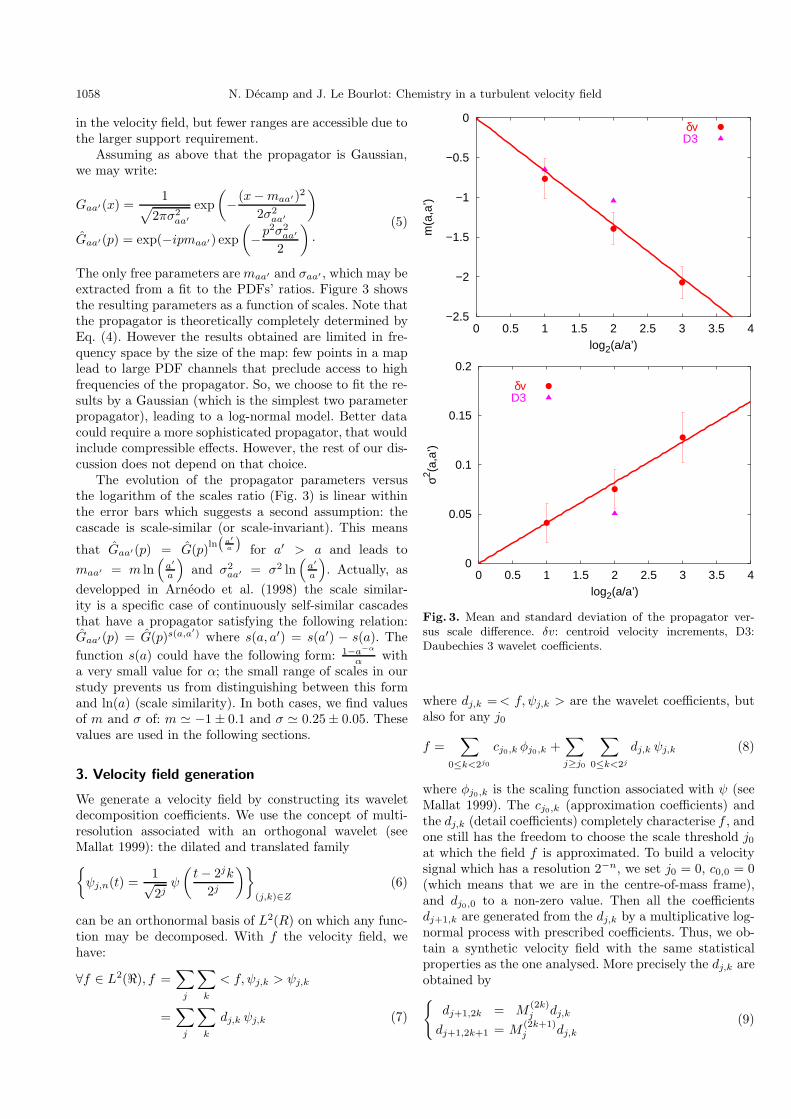
The only free parameters are maa′ and σaa′ , which may beextracted from a fit to the PDFs’ ratios. Figure 3 showsthe resulting parameters as a function of scales. Note thatthe propagator is theoretically completely determined byEq. (4). However the results obtained are limited in fre-quency space by the size of the map: few points in a maplead to large PDF channels that preclude access to highfrequencies of the propagator. So, we choose to fit the re-sults by a Gaussian (which is the simplest two parameterpropagator), leading to a log-normal model. Better datacould require a more sophisticated propagator, that wouldinclude compressible effects. However, the rest of our dis-cussion does not depend on that choice.

The evolution of the propagator parameters versusthe logarithm of the scales ratio (Fig. 3) is linear withinthe error bars which suggests a second assumption: thecascade is scale-similar (or scale-invariant). This means

that Gaa′(p) = G(p)ln(a′a

)for a′ > a and leads to

maa′ = m ln(a′

a

)and σ2

aa′ = σ2 ln(a′

a

). Actually, as

developped in Arneodo et al. (1998) the scale similar-ity is a specific case of continuously self-similar cascadesthat have a propagator satisfying the following relation:Gaa′(p) = G(p)s(a,a

′) where s(a, a′) = s(a′) − s(a). Thefunction s(a) could have the following form: 1−a−α

α witha very small value for α; the small range of scales in ourstudy prevents us from distinguishing between this formand ln(a) (scale similarity). In both cases, we find valuesof m and σ of: m ' −1± 0.1 and σ ' 0.25± 0.05. Thesevalues are used in the following sections.

3. Velocity field generation

We generate a velocity field by constructing its waveletdecomposition coefficients. We use the concept of multi-resolution associated with an orthogonal wavelet (seeMallat 1999): the dilated and translated family{ψj,n(t) =

1√2jψ

(t− 2jk

2j

)}(j,k)∈Z

(6)

can be an orthonormal basis of L2(R) on which any func-tion may be decomposed. With f the velocity field, wehave:

∀f ∈ L2(<), f =∑j

∑k

< f,ψj,k > ψj,k

=∑j

∑k

dj,k ψj,k (7)

−2.5

−2

−1.5

−1

−0.5

0

0 0.5 1 1.5 2 2.5 3 3.5 4

m(a

,a’)

log2(a/a’)

δvD3

0

0.05

0.1

0.15

0.2

0 0.5 1 1.5 2 2.5 3 3.5 4

σ2 (a,a

’)

log2(a/a’)

δvD3

Fig. 3. Mean and standard deviation of the propagator ver-sus scale difference. δv: centroid velocity increments, D3:Daubechies 3 wavelet coefficients.

where dj,k =< f,ψj,k > are the wavelet coefficients, butalso for any j0

f =∑

0≤k<2j0

cj0,k φj0,k +∑j≥j0

∑0≤k<2j

dj,k ψj,k (8)

where φj0,k is the scaling function associated with ψ (seeMallat 1999). The cj0,k (approximation coefficients) andthe dj,k (detail coefficients) completely characterise f , andone still has the freedom to choose the scale threshold j0at which the field f is approximated. To build a velocitysignal which has a resolution 2−n, we set j0 = 0, c0,0 = 0(which means that we are in the centre-of-mass frame),and dj0,0 to a non-zero value. Then all the coefficientsdj+1,k are generated from the dj,k by a multiplicative log-normal process with prescribed coefficients. Thus, we ob-tain a synthetic velocity field with the same statisticalproperties as the one analysed. More precisely the dj,k areobtained by{

dj+1,2k = M(2k)j dj,k

dj+1,2k+1 = M(2k+1)j dj,k

(9)


−7

−6

−5

−4

−3

−2

−1

0

0 2 4 6 8 10 12 14

ln(σ

l(v))

log2(l)

ModelPolaris

Gaussian field

Fig. 4. Standard deviation of the velocity field as a functionof size l (in pixel units) for Polaris, for the synthetic field, andfor a Gaussian field. The vertical offset of the model is fixedby d0,0. Straight lines are power laws with an exponent β = 0.5.

where∣∣∣M (k)

j

∣∣∣ are realisations of a random variable Mj

that follow the log-normal law from Sect. 2.2 with a =2−j and a′ = 2−j−1. Numerical values of the velocity areexpressed in units of dj0,0.

The standard deviation of the velocity field as a func-tion of size is plotted in Fig. 4. The law σl(v) ∝ lβ fitsboth the synthetic velocity field and the Polaris regionwell with an exponent of β ' 0.5 in both cases. This ex-ponent is clearly irrelevant (or equal to 0) for a classicalGaussian field: for such a field the standard deviation isthe same for any scale; the difference observed is just asampling effect. The model is adjusted to observations byfixing d0,0 so that the curves coincide. Here, d0,0 = 250 for13 octaves (reductions of scale by a factor of 2) betweenthe integral scale and the ∆ = 2 scale.

The resulting velocity field is then submitted to thesame analysis as the original one, and the number ofsteps between our integral scale and the Polaris map scaleis fixed by adjusting the non-Gaussian wings. Figure 5shows the resulting PDFs. Here N = 13 between the in-tegral scale and the ∆ = 2 scale. Note that the syntheticfield PDFs are in good agreement with the observed ones,and that the synthetic field is correlated at all scales (arough estimate of the synthetic signal correlation lengthat scale a is a) unlike the uncorrelated Gaussian field usedfor comparisons.

We are now able to determine the scaling of our modelby identifying size at scale N with Polaris resolution. InFig. 5, ∆ = 2 pixels corresponds to lN = 2250 AU, sothat our integral scale is l0 = 2N .2250 AU = 90 pc. Notethat this is not the size of the cloud that we generate: thePolaris map size is reached after 9 steps in the generatingprocess. A side effect of that sub-sampling is that the meanglobal velocity of the generated cloud is slightly non 0.0(see Sect. 4.4).

0.01

0.1

1

10

0.4 0.2 0 0.2 0.4

ln(P

(δv)

)

δ∆v = v(x+∆) v(x)

∆=2∆=4∆=8

Gaussian

Fig. 5. Comparison between the velocity increments’ PDFs ofthe Polaris map (points) and the reconstructed field (lines) fordifferent scales.

4. One-dimensional model

4.1. Why a cellular automata

The use of a wavelet decomposition of our synthetic ve-locity field gives access to the best approximation at anyscale between the integral scale l0 (where it is just themean velocity, and is 0.0 by construction) and the small-est accessible scale l0 2−Nmax , where Nmax is the numberof steps in the wavelet transform.

As we are interested in the effects of turbulence onthe dynamics of a cloud, the smallest significant scale isthe turbulence dissipation length. Any cell of gas smallerthan that length is homogeneous and statistically iden-tical to its nearest neighbour. That scale may be esti-mated from classical results on Kolmogorov turbulence(see Frisch 1995): the energy flux through scales is ε = v3

l ,which is true also at lN , the Polaris resolution scale withvN , the turbulent velocity at that scale. We can estimatethat quantity from the observations if we take ∆v, thestandard deviation of centroids increments at scale lN , asan estimate of vN . From the Polaris map, vN = 0.1kms−1,so that ε = 3×10−5 cm2 s−3. Then the dissipation scale is

given by η =(ν3

ε

)1/4

, where ν is the kinematic viscosity.In a diluted gas, ν ' vth

nσ , where vth is the thermal velocity,n the gas density, and σ the collision cross section. Insidea molecular gas, we can take a mean H2–H2 cross sectionof σ = 1.5 × 10−14 cm2 (see Le Bourlot et al. (1999)),a density of 104 cm−3 and a temperature of 10 K. Thisgives:

η = 7.5× 1011( n

104

)−3/4(

ε

3× 10−5

)−1/4 (T

10

)3/8

cm.

From lN , we can proceed with the cascade process downto the smallest scale lNmax that depends mainly on com-putational power. However, lN

η ∼ 215, which is stilltoo much for us. We have chosen to stop the model atlNmax = 140 AU (Nmax = 17). The corresponding angular


resolution at Polaris would be 0.94′′. The associated timescale is tNmax = lNmax

vNmax= 5.25×1011 s (note that the effec-

tive velocity dispersion at that scale vNmax ' 0.04 kms−1

is close to the value deduced from a constant ε up to thatscale).

Since we are not interested in the physics inside thatbox, we can use a coarse-grained approximation by look-ing at a collection of identical cells of size lNmax , coupledby convection (hence our need to prescribe the velocityfield) or radiatively (i.e. in velocity space nearest neigh-bour but not necessarily in physical space, see Rousseauet al. 1998). Thus, we by-pass the need to solve partialdifferential equations and need only to prescribe the evo-lution of mean variables inside each box and their mutualcoupling (hereafter only by convection). The most accu-rate way to realise that smoothing is to use the approxi-mation coefficients of the wavelet transform at that scale.

So we consider a set of identical boxes, each charac-terised by local dynamics (a set of local variables, coupledby physical relationships) with the same variables and evo-lution laws in each cell, but not necessarily the same ini-tial conditions. Evolution is computed over a continuoustime within each box, and a spatial coupling is appliedat discrete times. The velocity at the smallest scale lNmax

is taken as the mean velocity of a box in a rest frame.Therefore we use an Eulerian representation. Velocity isprescribed a priori, and is not modified by the evolutionof any local variable. It is understood that the way thevelocity field is built takes care of all (mostly unknown)processes that constrain its evolution. What we need nowis a way to progress in time.

4.2. Time dependence

As a first stage, our goal is to model a cloud in steadystate. This means that all its statistical properties remainconstant on average, but are not necessarily time indepen-dent! They may fluctuate in time around a mean value,and only that value is constant in time. This has to betrue also for the velocity field, so that we need to pre-scribe the evolution in time of the static field of Sect. 3.To that end, we make the hypothesis that turbulence ishomogeneous, isotropic, and stationary. Under these threeconditions, the Taylor hypothesis applies and the statisti-cal properties of v(x0, t) as t varies are the same as those ofv(x, t0) along an axis x. This hypothesis may be extendedto a 1D structure: the statistical properties of a velocityfield v(X, t) along an axis X as t varies are the same asthat of a collection of lines in a 2D plane at a given time t0.The second hypothesis is stronger than the first becausecross-correlations between orthogonal directions X and Yhave to be included and is only true if the three conditionsof homogeneity, isotropy, and stationarity strictly apply,see Appendix A for a demonstration.

The extension to 2D of the velocity field generation al-gorithm is straightforward (although computationally in-tensive). Details are given in Arneodo et al. (1999) and

references therein (see Appendix C). Once a 2D X–Yfield has been generated, the Y axis can be interpretedas u0t, where u0 is a “scanning” velocity that sets a timescale for the model. For consistency, we take u0 = vNmax .From this point, the velocity in our model is prescribed ineach box of size δ = lNmax = l0 2−Nmax and at each timetj = j tNmax = j δ

vNmax(where tNmax = 5.25× 1011 s is the

crossing time at the smallest scale).

4.3. Density field

Mass conservation reads:

∂ρ

∂t+−→∇.(ρ−→v ) = 0. (10)

Once the velocity field is known (which is our case), thisequation becomes a linear PDE in only one unknown, ρ.It can be solved easily as soon as initial and boundaryconditions are set. The system is dissipative and a typicalstationary state is reached after a relaxation time of afew tNmax (with tNmax = 5.25× 1011 s).

We use uniform initial conditions and assume peri-odic boundary conditions. Equation (10) is solved in each“box” as a balance equation. We “count” the total amountof matter that escapes and enters each box: namely, forthree successive boxes (at step j, density ρji−1, ρji and ρji+1

and velocity vji−1, vji and vji+1, we have:

ρj+1i =ρji−1

vji−1

u0Y +i−1 +ρji

1−

∣∣∣vji ∣∣∣u0

−ρji+1

vji+1

u0Y −i+1(11)

where Y +i = 1 if vi is positive, Y −i = 1 if vi is negative,

and both are zero otherwise. Within a time step tNmax ,the number of sub-step k is chosen to ensure that vi

k u0stays lower than 1 (as a further development, the methodmay include asynchronous time integration). Note thatthe absolute value of the density scaling is arbitrary, sincevelocity evolution does not depend on it; all density fieldsfollow the same evolution.

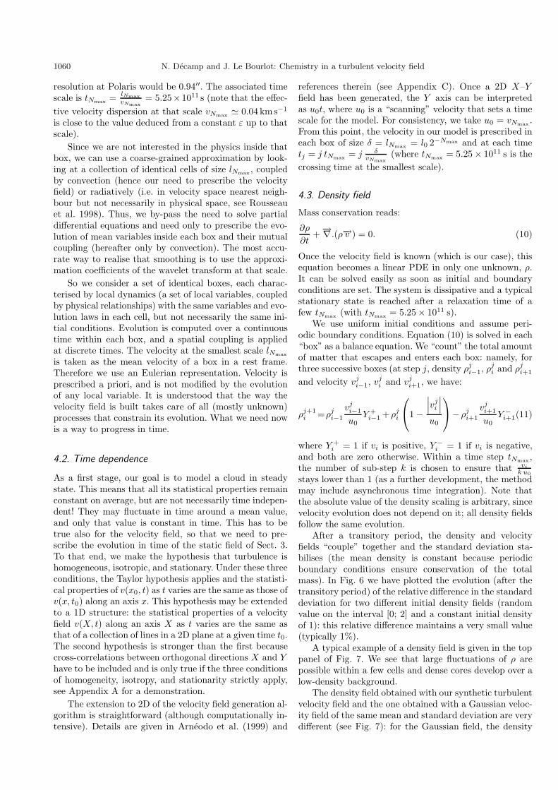
After a transitory period, the density and velocityfields “couple” together and the standard deviation sta-bilises (the mean density is constant because periodicboundary conditions ensure conservation of the totalmass). In Fig. 6 we have plotted the evolution (after thetransitory period) of the relative difference in the standarddeviation for two different initial density fields (randomvalue on the interval [0; 2] and a constant initial densityof 1): this relative difference maintains a very small value(typically 1%).

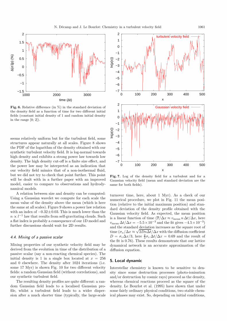
A typical example of a density field is given in the toppanel of Fig. 7. We see that large fluctuations of ρ arepossible within a few cells and dense cores develop over alow-density background.

The density field obtained with our synthetic turbulentvelocity field and the one obtained with a Gaussian veloc-ity field of the same mean and standard deviation are verydifferent (see Fig. 7): for the Gaussian field, the density


−1.5

−1

−0.5

0

0.5

1

1.5

2

1000 2000 3000

∆(σ)

(ρ)

(%)

time (∆t)

Fig. 6. Relative difference (in %) in the standard deviation ofthe density field as a function of time for two different initialfields (constant initial density of 1 and random initial densityin the range [0; 2]).

seems relatively uniform but for the turbulent field, somestructures appear naturally at all scales. Figure 8 showsthe PDF of the logarithm of the density obtained with oursynthetic turbulent velocity field. It is log-normal towardshigh density and exhibits a strong power law towards lowdensity. The high density cut-off is a finite size effect, andthe power law may be interpreted as an indication thatour velocity field mimics that of a non-isothermal fluid,but we did not try to check that point further. This pointwill be dealt with in a further paper with an improvedmodel, easier to compare to observations and hydrody-namical models.

A relation between size and density can be computed:Using a Gaussian wavelet we compute for each scale themean value of the density above the mean (which is herethe same at all scales). Figure 9 shows a power law relationwith an index of −0.32±0.03. This is much lower than then ∝ l−1 law that results from self-gravitating clouds. Sucha flat index is probably a consequence of our 1D model andfurther discussions should wait for 2D results.

4.4. Mixing of a passive scalar

Mixing properties of our synthetic velocity field may bederived from the evolution in time of the distribution of apassive scalar (say a non-reacting chemical species). Theinitial density is 1 in a single box located at x = 256and 0 elsewhere. The density after 1024 iterations (i.e.some 17 Myr) is shown Fig. 10 for two different velocityfields: a random Gaussian field (without correlations), andour synthetic turbulent field.

The resulting density profiles are quite different: a ran-dom Gaussian field leads to a localised Gaussian pro-file, whilst a turbulent field leads to a wider disper-sion after a much shorter time (typically, the large-scale

−7

−6

−5

−4

−3

−2

−1

0

1

2

0 100 200 300 400 500

ln(ρ

(x))

x

turbulent velocity field

−7

−6

−5

−4

−3

−2

−1

0

1

2

0 100 200 300 400 500

ln(ρ

(x))

x

Gaussian velocity field

Fig. 7. Log of the density field for a turbulent and for aGaussian velocity field (mean and standard deviation are thesame for both fields).

turnover time, here, about 1 Myr). As a check of ournumerical procedure, we plot in Fig. 11 the mean posi-tion (relative to the initial maximum position) and stan-dard deviation of the density profile obtained with theGaussian velocity field. As expected, the mean positionis a linear function of time (x/∆x ≈ vmean n∆t/∆x, herevmean ∆t/∆x = −5.5×10−3 and the fit gives −4.5×10−3)and the standard deviation increases as the square root oftime (σx/∆x ≈

√2Dn∆t/∆x with the diffusion coefficient

D = σv∆x/3, here 23σv ∆t/∆x = 0.69 and the result of

the fit is 0.76). These results demonstrate that our latticedynamical network is an accurate approximation of thediffusion equation.

5. Local dynamic

Interstellar chemistry is known to be sensitive to den-sity since some destruction processes (photo-ionisationand/or destruction by cosmic rays) proceed as the density,whereas chemical reactions proceed as the square of thedensity. Le Bourlot et al. (1995) have shown that undersome fairly ordinary physical conditions, two stable chem-ical phases may exist. So, depending on initial conditions,


10−4

10−3

10−2

10−1

100

−12 −10 −8 −6 −4 −2 0 2

pdf(

n)

log(n(A))

Turbulent velocity field

Fig. 8. Pdf of the logarithm of the density for our turbulentvelocity field.

0.35

0.4

0.45

0.5

0.55

0.6

0.65

0.7

0.75

0.8

0.85

0.9

0 0.2 0.4 0.6 0.8 1 1.2 1.4 1.6

log(

r)

log(l)

total densitylinear fit

Fig. 9. Decimal logarithm of the density as a function of scale.

some parts of the cloud may evolve towards one phase asothers evolve towards the other phase. Interfaces betweenthose phases lead to reaction-diffusion fronts where un-usual chemical abundances may prevail for long times ina manner similar to reaction-diffusion fronts in a thermallybistable fluid studied by Shaviv & Regev (1994).

Thus, a minimal local dynamic should at least exhibitbistability. This can be achieved with a 3-variable modelwhich is the minimal non-passive scalar model possible.By turning on or off turbulent mixing, we can test theeffects of that mixing on mean abundances along the lineof sight and on time and length scales for each variablewithin the cloud.

This is an extension to intrinsically scale-dependentmodels of the work of Xie et al. (1995) and Chieze &Des Forets (1989). However, full-size interstellar chemicalschemes are still beyond our reach.

-50

-40

-30

-20

-10

0

0 100 200 300 400 500

ln(ρ

(x))

x

Gaussian fieldturbulent field

fit

Fig. 10. Dispersion of a passive scalar (after 1024 iterations oftNmax = 5.25× 1011 s) by our synthetic turbulent field and bya Gaussian field (mean and standard deviation of the velocityfield are the same for both fields). Point source released at t = 0at x = 256.

As a test model, we chose the following set of chemicalreactions (inspired from Gray & Scott 1990):

R → A (k1)A → B (k2)

A+ 2B→3B (k3)B → P (k4)·

(12)

Such a model can be seen as an excerpt from a larger chem-ical network with R = R′ρ, being a production term pro-portional to the density, and where the product(s) P re-turns to the rest of the gas.

If we suppose that k1 has the following tempera-ture dependence k1 = k10 exp(− Ea

kbT) and that reac-

tion (4) is exothermic, then thermal balance is gov-erned by: ∆U = k4∆t∆HnB − k5kb∆t(nA + nB)T (withU = ρcp,ρT = nRcp,RT ). Here the cooling term mimicsradiative cooling by both A and B after collisionalexcitation.

We can reduce the problem to a simple dynamical sys-tem with three differential equations and four parame-ters (r, ε, k, γ):

dαdτ

= r exp(−εru

)− kα− αβ2

dβdτ

= kα+ αβ2 − β

dudτ

= β − γ(α+ β)ur

(13)


−100

−80

−60

−40

−20

0

20

40

60

80

0 1000 2000 3000 4000 5000 6000 7000 8000

mea

n(t)

t

Gaussian fieldlinear fit

turbulent field

0

20

40

60

80

100

120

0 500 1000 1500 2000 2500 3000 3500 4000

σ(t)

t

Gaussian fieldy(t)= a * √t

turbulent field

Fig. 11. Temporal evolution of the mean and standard devia-tion of the passive scalar density distribution for our two fields.As expected for diffusion by a Gaussian field, the mean andvariance are proportional to time.

with

α=√k3

k4nA

β=√k3

k4nB

u=U

∆H

√k3

k4τ = k4t

r=k10

k4

√k3

k4nR

ε=Eacp,R k4

k10kb∆Hk=

k2

k4

γ=k5kbk10

cp,R k24

·

(14)

This simple dynamical system leads to many different situ-ations: bistability or limit cycle with Hopf bifurcation (seeFig. 12) for different parameters3. In the following, we use

3 Figure 12 was created using the software packageCANDYS/QA by W. Jansen. Seehttp://www.agnld.uni-potsdam.de/~wolfgang/ca-inst.html

0.01

0.1

1

10

0.1 1 10 100

α

r

stable st−stHopf bifurcation

unstable st−stturning point

0.0001

0.001

0.01

0.1

1

10

100

0.1 1 10 100

b

r

stable st-stHopf bifurcation

unstable st-stturning point

Fig. 12. An example of bistability and limit cycle with Hopfbifurcation. The parameters values are k = 0.001, γ = 1, ε =0.01. We plotted the values of α and β, at the equilibrium, fordifferent values of the r parameter (x axis).

k = 0.001, r = 1, γ = 1 and ε = 0.01 as our referencebistable model. The chemical time scale is 1/k4, so thatthe ratio of turbulent to chemical time scales is k4tNmax .In the following, we usually use k4tNmax = 0.1 (tNmaxbeingthe crossing time at the smallest scale we resolve).

6. Reactive medium in turbulent flow

It is then possible to add the effects of that non-triviallocal dynamic to turbulent mixing. We select the modelof Sect. 5. In order to study the influence of the turbu-lence, we again do a comparison between a turbulent anda Gaussian velocity field (Fig. 13 for one example). Notethat A, B (chemical species), U (internal energy) and R(proportional to the total density) are advected as de-scribed by Eq. (11) extended to 4 variables.

We can observe that, as in the previous case (Sect. 4.3),structures appear naturally at all scales in the turbulentcase and not with a Gaussian velocity field. Appendix Dshows the variations of A on a much larger time scale.Different initial conditions give indistinguishable results,suggesting that steady state is reached. However, we can-not exclude that some long time drift may still exist whichour computation is unable to uncover.

Turbulent structures are not the same for the differentcomponents (A, B, R) neither in position nor in size, ascan be seen in Fig. 14, which is an horizontal cut of Fig. 13.In order to study more precisely these effects, we plot the


Fig. 13. Density of component A (see Eq. (12)) in a bistablecase. The horizontal axis represents position and time flowsfrom top to bottom, using the same initial conditions. Only thelatest iterations are shown. Lowest densities are deep blue andhighest densities light red. Top panel: mixing by a Gaussianvelocity field; bottom panel: mixing by a turbulent field (seeAppendix D for a much longer time evolution).

probability density function of A (Fig. 15) which shouldbe compared to Fig 8.

Note that the presence of a non-uniform velocity fieldleads to a single-peaked broad distribution. Turbulenceleads to a broader distribution and extended wings. Thusthe probability to find some regions at far from equilib-rium values is enhanced.

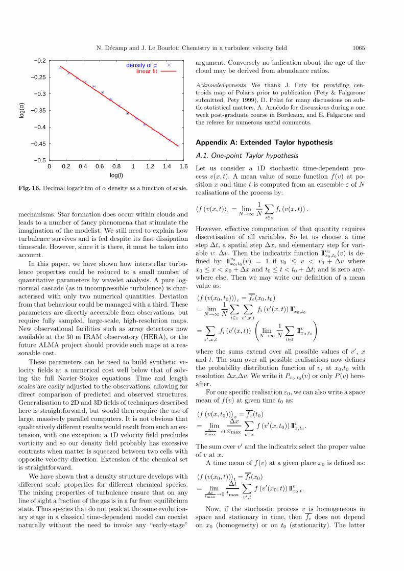
We also plotted the density of α =√

k3k4nA as a func-

tion of size (see Fig. 16) using the same procedure as forFig. 9. The slope is −0.17± 0.03 (instead of −0.32± 0.03for the total density, cf. Sect. 4.3). The evolution throughscales is therefore significantly different for one particularcomponent and for the total density.

0

10

20

30

40

50

60

0 100 200 300 400 500

ρ(x)

x

R componentA component (× 20)

Fig. 14. Density of components A and R as a function of po-sition at a given time (last time step of Fig. 13 i.e. last “line”),for a turbulent field.

10−5

10−4

10−3

10−2

10−1

100

−12 −10 −8 −6 −4 −2 0 2

pdf(

n)

log(n(A))

GaussianTurbulent

Fig. 15. Probability density function of A for two differentvelocity fields: a Gaussian random field and a turbulent velocityfield.

7. Discussion

The structure of interstellar clouds remains a subject ofdebate because different observations suggest different,and often contradictory, interpretations. The Thoravalet al. (1999) results, based on infrared observations aresensitive mainly to the dust distribution and thus proba-bly to the bulk of the mass distribution. On the contrary,some low-abundance species (see for example Marscheret al. 1993 and Moore & Marscher 1995 results) exhibitlarge abundance variations down to the smallest accessiblescales.

Our results show that the structuring of the gas bythe turbulent velocity field leads naturally to different dis-tributions for different species, without requiring any ex-ternal mechanism. Thus, seemingly contradictory obser-vations find a unified explanation which applies to anyturbulent region in the interstellar medium. Naturally,this does not preclude a significant influence of other


−0.5

−0.45

−0.4

−0.35

−0.3

−0.25

−0.2

0 0.2 0.4 0.6 0.8 1 1.2 1.4 1.6

log(

α)

log(l)

density of αlinear fit

Fig. 16. Decimal logarithm of α density as a function of scale.

mechanisms. Star formation does occur within clouds andleads to a number of fancy phenomena that stimulate theimagination of the modelist. We still need to explain howturbulence survives and is fed despite its fast dissipationtimescale. However, since it is there, it must be taken intoaccount.

In this paper, we have shown how interstellar turbu-lence properties could be reduced to a small number ofquantitative parameters by wavelet analysis. A pure log-normal cascade (as in incompressible turbulence) is char-acterised with only two numerical quantities. Deviationfrom that behaviour could be managed with a third. Theseparameters are directly accessible from observations, butrequire fully sampled, large-scale, high-resolution maps.New observational facilities such as array detectors nowavailable at the 30 m IRAM observatory (HERA), or thefuture ALMA project should provide such maps at a rea-sonable cost.

These parameters can be used to build synthetic ve-locity fields at a numerical cost well below that of solv-ing the full Navier-Stokes equations. Time and lengthscales are easily adjusted to the observations, allowing fordirect comparison of predicted and observed structures.Generalisation to 2D and 3D fields of techniques describedhere is straightforward, but would then require the use oflarge, massively parallel computers. It is not obvious thatqualitatively different results would result from such an ex-tension, with one exception: a 1D velocity field precludesvorticity and so our density field probably has excessivecontrasts when matter is squeezed between two cells withopposite velocity direction. Extension of the chemical setis straightforward.

We have shown that a density structure develops withdifferent scale properties for different chemical species.The mixing properties of turbulence ensure that on anyline of sight a fraction of the gas is in a far from equilibriumstate. Thus species that do not peak at the same evolution-ary stage in a classical time-dependent model can coexistnaturally without the need to invoke any “early-stage”

argument. Conversely no indication about the age of thecloud may be derived from abundance ratios.

Acknowledgements. We thank J. Pety for providing cen-troids map of Polaris prior to publication (Pety & Falgaronesubmitted, Pety 1999), D. Pelat for many discussions on sub-tle statistical matters, A. Arneodo for discussions during a oneweek post-graduate course in Bordeaux, and E. Falgarone andthe referee for numerous useful comments.

Appendix A: Extended Taylor hypothesis

A.1. One-point Taylor hypothesis

Let us consider a 1D stochastic time-dependent pro-cess v(x, t). A mean value of some function f(v) at po-sition x and time t is computed from an ensemble ε of Nrealisations of the process by:

〈f (v(x, t)〉ε = limN→∞

1N

∑i∈ε

fi (v(x, t)) .

However, effective computation of that quantity requiresdiscretisation of all variables. So let us choose a timestep ∆t, a spatial step ∆x, and elementary step for vari-able v: ∆v. Then the indicatrix function IIv0

x0,t0(v) is de-fined by: IIv0

x0,t0(v) = 1 if v0 ≤ v < v0 + ∆v wherex0 ≤ x < x0 + ∆x and t0 ≤ t < t0 + ∆t; and is zero any-where else. Then we may write our definition of a meanvalue as:

〈f (v(x0, t0))〉ε = fε(x0, t0)

= limN→∞

1N

∑i∈ε

∑v′,x,t

fi (v′(x, t)) IIvx0,t0

=∑v′,x,t

fi (v′(x, t))

(limN→∞

1N

∑i∈ε

IIvx0,t0

)

where the sums extend over all possible values of v′, xand t. The sum over all possible realisations now definesthe probability distribution function of v, at x0,t0 withresolution ∆x,∆v. We write it Px0,t0(v) or only P (v) here-after.

For one specific realisation ε0, we can also write a spacemean of f(v) at given time t0 as:

〈f (v(x, t0))〉x = fx(t0)

= lim∆xxmax

→0

∆xxmax

∑v′,x

f (v′(x, t0)) IIvx,t0 .

The sum over v′ and the indicatrix select the proper valueof v at x.

A time mean of f(v) at a given place x0 is defined as:

〈f (v(x0, t))〉t = ft(x0)

= lim∆ttmax

→0

∆ttmax

∑v′,t

f (v′(x0, t)) IIvx0,t.

Now, if the stochastic process v is homogeneous inspace and stationary in time, then fε does not dependon x0 (homogeneity) or on t0 (stationarity). The latter


hypothesis requires that our process be dissipative andthat any initial condition be forgotten, that is tmax shouldbe large compared to all characteristic time scales of theprocess. By the same argument, fx does not depend on t0,and ft does not depend on x0.

That these three mean values are the same followsBirkhoff’s ergodic theorem, as developed in Frisch (1995)Chapters 3 and 4. Therefore, we get fx = ft, which is theTaylor hypothesis.

If v is a 3D phenomenon, then isotropy is further re-quired to chose at random a direction x so that the resultis independent of that specific direction. Note that the ar-gument does not depend on the choice of f , which can beany function of the stochastic process v, thus it is true forall moments of the process v itself, whatever its distribu-tion function (Gaussian or not Gaussian).

Stationary developed turbulence is supposed to be ho-mogeneous and isotropic so that this result applies for anycomponent of the velocity field.

A.2. Extended Taylor hypothesis

Now let us consider a 2D stochastic process v. Usingisotropy, we select a random direction x to which y isorthogonal. Then, we choose a segment Sy0 along x at y0.Again, space is discretised by ∆x = ∆y, time by ∆t, andv (assumed scalar) by ∆v. All previous results apply toany one-point function of v, that is any mean quantity isindependent of the choice of y0 (homogeneity), of any x0

along Sy0 (homogeneity again), of time (stationarity) orof the choice of the initial direction (isotropy).

However, we may also define on Sy0 two-point (ormore) functions that are not taken care of by the pre-vious results. For two points x1 and x2 along Sy0 suchthat |x2 − x1| = L, we have:

〈f (v1(x1, t0), v2(x2, t0))〉x = fx(L)

= lim ∆xxmax

→0

∆xxmax

∑v′1,x1,v′2,x2

f(v′1(x1, t), v′2(x2, t)) IIv1x,t0IIv2

x,t0

and an analogous expression for ft(L). But now, if L isshorter than any spatial correlation length of the pro-cess v, then the expression for fx(L) does not factorise,since events at x1 and x2 are not independent. However,it remains independent of y0, x1 and x2 separately, and t0.Only the distance L between the two points matters. Bythe same argument, ft(L) is also independent of y0, andx1 and x2 separately. We may again apply Birkhoff’s the-orem, and state that fx(L) = ft(L).

Strictly speaking, a third mean value can be defined,which is fy(L), for two points separated by L along di-rection x, but with samples taken out of parallel seg-ments Sy along y. For a scalar process, isotropy ensuresthat fx(L) = fy(L). We assume here that the same is truefor any component of the velocity field, thus neglectingthe possible effect of cross-correlations.

Within that restriction, we see that, providing all sizesconsidered are large with respect to the largest correla-tion size within our sample, the same reasoning leads to a

value of f(L) independent of the fact that we computed aspatial mean, or a temporal mean (in the same way thatwe needed to consider time scales large with respect tothe largest correlation time to get the usual Taylor hy-pothesis). This is again independent of the choice of thefunction f and can be generalised to any number of points(or any order).

Thus we see that statistical properties of v along asegment S as time flows are the same as the statisticalproperties of a family of parallel segments in space at agiven time. By choosing a “scanning velocity” u0, we areable to transform a 2D static field v(x, y) into a 1D, timevarying field v(x, t = y/u0).

Appendix B: Centroid velocity increments

The centroid velocity (C) is the mean radial velocity: if wecall T (u) the intensity as a function of the radial velocity,then by definition C =

(∫uT (u)du

)/(∫T (u)du

). In the

case of an optically thin medium, T (u) ∝ N(u), whereN(u) is the column density as a function of the radial ve-locity (N(u) =

∫ s00n(u)ds). It is then easy to show that

C =(∫u(s)n(s)ds

)/N . This quantity is very commonly

used because of the lack of information about the velocityspatial repartition along the line of sight. The centroid ve-locity increment at scale a is then: δCa = C(r+a)−C(r),where r is a position on the plane of the sky. The prob-ability density function (PDF) of this quantity in a tur-bulent velocity field is essentially indistinguishable froma Gaussian for the integral scale and develops more andmore non-Gaussian wings as the lag decrease (see Lis et al.1996; Pety 1999; Miesch et al. 1999).

Appendix C: 2D log-normal cascade

For any function f ∈ L2per([0, L]2), f can be written under

the form

f(x, y) =N∑j=0

2N−j−1∑m,n=0

3∑k=0

ckj,m,nψkj,m,n(x, y).

The construction rule is the following: one generates the

modulus dj,m,n =([c1j,m,n

]2 +[c2j,m,n

]2 +[c3j,m,n

]2)1/2

of the wavelet coefficients in a recursive way by:

dj−1,2m,2n = M(1)j,m,ndj,m,n

dj−1,2m+1,2n = M(2)j,m,ndj,m,n

dj−1,2m,2n+1 = M(3)j,m,ndj,m,n

dj−1,2m+1,2n+1 = M(4)j,m,ndj,m,n.

Mj,m,n follows the prescribed log-normal law (m,σ).The wavelet coefficients themselves are computed via

two angles (θ, φ):c1j,m,n = cos(φ) cos(θ)dj,m,n

c2j,m,n = cos(φ) sin(θ)dj,m,n

c3j,m,n = sin(φ)dj,m,n


where θ is randomly chosen between [−π, π] and φ israndomly chosen between [−φ∗, φ∗] where φ∗satisfies

sin (2φ∗)4φ∗

=2τ(2)/2+3

1 + 2τ(2)/2+3− 1

2

with

τ(q) = −σ2

2q2 −mq − 2.

Finally, isotropy follows from adjusting the weights at thelargest scale:c10,0,0 = d0,0,0, c20,0,0 = d0,0,0, and c30,0,0 = 2−(τ(2)/4+1)d0,0,0

(see Decoster et al. 2000 for all details).

Appendix D: Evolution on large time scales

We give in Figs. D.1 to D.4 the evolution of the α densitywith the same turbulent field and the same parameters asin Fig. 13 but on a larger time scale.

References

Arneodo, A., Muzy, J. F., & Roux, S. G. 1997, J. Phys. IIFrance, 7, 363

Arneodo, A., Manneville, S., & Muzy, J. F. 1998, Eur. Phys.J. B, 1, 129

Arneodo, A., Decoster, N., & Roux, S. G. 1999, Phys. Rev.Lett., 83, 1255

Ballesteros-Paredes, J., Vazquez-Semadeni, E., & Scalo, J.1999, ApJ, 515, 286

Castaing, B. 1996, J. Phys. II France, 6, 105Chieze, J. P., & Pineau des Forets, G. 1989, A&A, 221, 89Decoster, N., Roux, S. G., & Arneodo, A. 2000, Eur. Phys. J.

B, 15, 739Falgarone, E., Lis, D. C., Phillips, T. G., et al. 1994, ApJ, 436,

728Falgarone, E., Panis, J.-F., Heithausen, A., et al. 1998, A&A,

331, 669Falgarone, E., & Phillips, T. G. 1990, ApJ, 359, 344Falgarone, E., Phillips, T. G., & Walker, C. K. 1991, ApJ, 378,

186Falgarone, E., & Puget, J.-L. 1995, A&A, 293, 840Frisch, U. 1995, Turbulence (Cambridge Univ. Press,

Cambridge)Gray, P., & Scott, S. K. 1990, Oxford Science Pub. (Clarendon

Press, Oxford)

Holzer, M., & Siggia, E. D. 1994, Phys. Fluids, 6, 1820Joulain, K., Falgarone, E., Pineau des Forets, G., & Flower, D.

1998, A&A, 340, 241Kegel, W. H., Piehler, G., & Albrecht, M. A. 1993, A&A, 270,

407Larson, R. B. 1981, MNRAS, 194, 809Le Bourlot, J., Pineau des Forets, G., & Roueff, E. 1995, A&A,

297, 251Le Bourlot, J., Pineau des Forets, G., & Flower, D. R. 1999,

MNRAS, 305, 802Lis, D. C., Pety, J., Phillips, T. G., & Falgarone, E. 1996, ApJ,

463, 623Lis, D. C., Keene, J., Li, Y., Phillips, T. G., Pety, J. 1998, ApJ,

504, 889Mac Low, M.-M., & Ossenkopf, V. 2000, A&A, 353, 339Mallat 1999, A wavelet tour of signal processing (Academic

Press)Marscher, A. P., Moore, E. M., & Bania, T. M. 1993, ApJ, 419,

L101Miesch, M. S., & Bally, J. 1994, ApJ, 429, 645Miesch, M. S., & Scalo, J. 1995, ApJ, 450, L27Miesch, M. S., Scalo, J., & Bally, J. 1999, ApJ, 524, 895Moore, E. M., & Marscher, A. P. 1995, ApJ, 452, 671Myers, P. C. 1983, ApJ, 270, 105Myers, P. C., & Khersonsky, V. K. 1995, ApJ, 442, 186Padoan, P., Bally J., Billawala, Y., Juvela, M., & Nordlundx,

A. 1999, ApJ, 525, 318Park, Y.-S., & Hong, S. S. 1995, A&A, 300, 890Pety, J. 1999, Ph.D. Thesis, Structures dissipatives de la tur-

bulence interstellaire : signatures cinematiques, UniversiteParis 6

Pety, J., & Falgarone, E. 2000, A&A, 356, 279Pety, J., & Falgarone, E., submitted to A&APiehler, G., & Kegel, W. H. 1995, A&A, 297, 841Rousseau, G., Chate, H., & Le Bourlot, J. 1998, MNRAS, 294,

373Scalo, J. M. 1987, in Interstellar Processes, ed. Hollenbach &

Thronson (Reidel Pub. Co.), 349Scalo, J. 1990, in Physical processes in Fragmentation and Star

Formation, ed. Capuzzo-Dolcetta et al. (Kluwer Ac. Pub.),151

Shaviv, N. J., & Regev, O. 1994, Phys. Rev. E, 50, 2048Stutzki, J., Bensch, F., Heithausen, A., Ossenkopf, V., &

Zielinsky, M. 1998, A&A, 336, 697Thoraval, S., Boisse, P., & Duvert, G. 1999, A&A, 351, 1051Vazquez-Semadeni, E., Passot, T., & Pouquet, A. 1995, ApJ,

441, 702Xie, T., Allen, M., & Langer, W. D. 1995, ApJ, 440, 674

interstellar turbulent velocity fields: scaling properties, synthesis and

Documents