Noname manuscript No.(will be inserted by the editor)

Intrackability: Characterizing Video Statistics and Pursuing VideoRepresentations

Haifeng Gong · Song-Chun Zhu

the date of receipt and acceptance should be inserted later

Abstract Videos of natural environments contain a widevariety of motion patterns of varying complexities whichare represented by many different models in the vision lit-erature. In many situations, a tracking algorithm is formu-lated as maximizing a posterior probability. In this paper,we propose to measure the video complexity by the entropyof the posterior probability, called the intrackability, to char-acterize the video statistics and pursue optimal video rep-resentations. Based on the definition of intrackability, ourstudy is aimed at three objectives. Firstly, we characterizevideo clips of natural scenes by intrackability. We calcu-late the intrackabilities of image points to measure the localinferential uncertainty, and collect the histogram of the in-trackabilities over the video in space and time as the globalvideo statistics. We found that the histograms of intracka-bilities can reflect the major variations, i.e., image scalingand object density, in natural video clips by a scatter plotof 2D PCA. Secondly, we show that different video repre-sentations, including deformable contours, tracking kernelswith various appearance features, dense motion fields, anddynamic texture models, are connected by the change of in-trackability and thus develop a simple criterion for modeltransition and for pursuing the optimal video representation.Thirdly, we derive the connections between the intrackabil-ity measure and other criteria in the literature such as theShi-Tomasi texturedness measure, conditional number, andcompare with Shi-Tomasi measure in tracking experiments.

Haifeng Gong was a postdoc researcher in the Department of Statistics,UCLA (2007-2009) and a researcher and team leader at Lotus Hill Re-search Institute, China during (2006-2010), and is a postdoc researcherat Computer and Information Science in University of Pennsylvaniasince 2009. This work was done when he was in Lotus Hill ResearchInstitute. Email address: hfgong@seas.upenn.edu.Song-Chun Zhu is a professor at the department of statistics and de-partment of computer science, UCLA and a founder of the Lotus HillInstitute, China. Email address: sczhu@stat.ucla.edu.

1 Introduction

1.1 Motivation and objective

Videos of natural environments contain a wide variety ofmotion patterns of varying complexities which are repre-sented by many distinct models in the vision literature. Fig. 1illustrates four typical representations: (i) A moving contourrepresenting a slowly walking human figure in near view;(ii) A kernel (window with interior feature points) repre-senting a fast moving car in middle distance; (iii) A densemotion (optical) flow field representing a marathon crowdmotion; and (iv) An appearance based spatio-temporal auto-regression (STAR) model representing the fire flame whereit is hard to track any distinct elements. The complexity ofthese video clips are affected by a few major factors, namely,the imaging scale, the object density, and the stochasticity ofthe motion. Apparently the change of these factors triggerstransitions among these representations. Fig. 2 shows twosequences of motion at distinct scales: the bird flock and themarathon crowd, where the individual bird or person is rep-resented by a contour, a kernel and a motion vector at threescales respectively.

These representations have been studied extensively forvarious tasks in the vision literature, for example, contourtracking (Maccormick and Blake, 2000; Sato and Aggarwal,2004; Black and Fleet, 2000), kernel tracking (Comani-ciu et al, 2003; Collins, 2003), PCA basis tracking (Rosset al, 2008; Kwon et al, 2009), motion vectors of points -– sparse (Shi and Tomasi, 1994; Tommasini et al, 1998;Segvic̀ et al, 2006; Serby et al, 2004; Veenman et al, 2001)or dense (Horn and Schunck, 1981; Ali and Shah, 2007),and dynamic texture (Szummer and Picard, 1996; Fitzgib-bon, 2001; Soatto et al, 2001) or textured motion (Wang andZhu, 2003). However, no attempt, to our best knowledge,has been made to formally characterize the video complex-

2

Dense flow fieldKernel Joint appearanceContour

(a) (b) (c) (d)

Fig. 1 Examples of motion patterns and their representations: (a) A slowly walking human figure at near view is represented by a contour; (b) Afast moving car in middle distance is represented by a kernel (window with multiple interior feature points); (c) A moving crowd in far view isrepresented by dense motion field; and (d) the dynamic texture of fire has no distinct element that is trackable, and is represented by auto-regressionmodels on its image intensities without explicit motion correspondence.

(a) (b) (c)

(a) (b) (c)

Fig. 2 The switch of video representations is triggered by image scaling (camera zooming) and density changes. (a) In high resolution, the birdshape and human figure are described by their contours; (b) In middle resolution, they are represented by a kernel with feature points; and (c) Inlow resolution, the people and birds are modeled by moving points with dense optical flow.

ity and to establish connections and conditions for the tran-sitions among these representations in the literature. In fact,the automated selection and switching of representations on-the-fly is of practical importance in real-time applications.For example, tracking an object over a long range of scaleswill need different representations. A surveillance systemmust also adapt its tracking task when the number of of tar-gets in a scene suddenly increases and cannot be trackedindividually due to limitation of computing resource. If thecomputing resource allows, it should output more detailedinformation for further processing, database indexing or hu-man inspection. When the number of objects at near distanceincreases, heavy occlusions always happen and we have tochange to track parts and discard some objects. When the

number of objects at far distance increases, we can changeto model motion flow and count number of objects. For ex-ample, (Ali and Shah, 2008) and (Cong et al, 2009) trackhigh density crowd scenes with motion field.

In this paper, we study an information theoretical crite-rion called the intrackability as a measure of the video com-plexity. By definition, the intrackability is the entropy of theposterior probability which a tracking or motion analysis al-gorithm tries to maximize, and thus reflects the difficultyand uncertainty in tracking certain elements (pixels, featurepoints, lines, patches). We will use the intrackability to char-acterize the video statistics, explain the transition betweenrepresentations, and pursue the optimal video representationfor an given video clip.

3

More specifically, our study is aimed at the followingthree objectives.

Firstly, we are interested in characterizing the global statis-tics of video clips and developing a panoramic map for thevariety of video representations. We calculate the intracka-bilities of some atomic image elements (patches) to measurethe local inferential uncertainty, and then we collect the his-togram of the intrackabilities over the video in space andtime as the global video statistics. We find that these his-tograms can be roughly decomposed in three bands whichcorrespond to three distinct motion regimes: (i) Low intrack-ability band for the trackable regime, which correspond toimage areas with distinct feature points or structured tex-ture areas that can be tracked with high accuracy. (ii) Highintrackability band for the intrackable regime, which cor-respond to image areas with no distinct texture, for exam-ple, flat areas or extremely populous areas. (iii) Medium in-trackability band which contains mostly texture areas wherestructures become less distinguishable. Using a PCA anal-ysis on these square root histograms, we find that the firsttwo eigen-vectors represent two major changes in the videospace: the transition between the trackable and the intrack-able motion and the transition between structure and texture.We plot the scatter plot and map natural video clips to thesetwo axes to gain some insights for the variations of videocomplexity.

Secondly, we are interested in developing an informa-tion theoretical criterion to guide the transition and selectionof video representations, in contrast to the common prac-tice that the video representations are manually selected fordifferent tasks. Our criterion is a sum of the intrackabilityof the tracked representation (W as a vector) and its com-plexity (the number of variables in W ). By minimizing thiscriterion (over W ), our algorithm automatically chooses anoptimal representation for the video clip which is often hy-brid – mixing various representations for different areas inthe video. In the spectrum of representations, the most com-plex one is the dense motion flow where each pixel or fea-ture point is tracked and W is a long vector, and the sim-plest one is the dynamic texture or textured motion whereno velocity is computed as there are no distinct and track-able elements and W is a short statistical description of themotion impression. Intuitively, when the ambiguity (or in-trackability) is large, we reduce the representationW by twoways: (i) dropping certain elements, for example, remove el-ements that are not trackable, or drop the motion directionin the tangent direction of a contour element; or (ii) merg-ing some descriptions, for example, combine a number offeature points that have similar motion in a kernel. In ex-periments, we show that different video representations, in-cluding deformable contours, tracking kernels with variousappearance features, dense motion fields, and spatial tempo-

ral auto-regression models are selected by the algorithm fordifferent video clips.

Thirdly, we compare our intrackability measure with threeother criteria in the literature: (i) the texturedness measurefor good features to track (Shi and Tomasi, 1994), (ii) Har-ris R score (Harris and Stephens, 1988) for corner detectionand (iii) the conditional number for robust tracking in (Fanet al, 2006). We show that all the three measures are relatedto different formula of the two eigenvalues in the local Gaus-sian distribution over the possible velocity. The intrackabil-ity is a general measure that are closely related to the threecriteria. We also compare the intrackability with Shi-Tomasimeasure by tracking experiments.

1.2 Related work in the literature

In the vast literature of motion analysis and tracking, thereare various criteria for feature selection (Marr et al, 1979;Dreschler and Nagel, 1981; Yilmaz et al, 2006). The cor-ner detector (Harris and Stephens, 1988) has been used fortracking feature selector for years. It is defined on eigenval-ues of a matrix collected from image gradients. For track-ing based on sum-of-squared-differences (SSD), (Shi andTomasi, 1994) selected good feature by a texturedness mea-sure which is also defined on the same matrix as (Harrisand Stephens, 1988). (Nickels and Hutchinson, 2002) an-alyzed variations of probability distributions of SSD motionvector, and measured the uncertainty in terms of covariancematrix from Gaussian fitting. For tracking based on kernels,(Fan et al, 2006) gave a reliability measure for kernel fea-ture based on condition number of a linear equation sys-tem. Covariance is also used in (Zhou et al, 2005) as anuncertainty measures for SSD, MeanShift and shape match-ing. For multi-frame adaptive tracking, (Collins et al, 2005)used log likelihood ratio scores of objects against the back-ground as a goodness measure. These measures are all asso-ciated with specified feature descriptions (e.g., SSD, kernel)and tracking model. A recent work (Pan et al, 2009) used aforward-backward tracking strategy to evaluate the robust-ness of a tracker — first the object is tracked forward for afew frames, then tracked backward from the end frame offorward tracking to the beginning one, and the difference ofthe initial position and the backward tracked result is usedas a measure of the robustness.

Our work is closely related to image scale-space theory,which was proposed by (Witkin, 1983) and (Koenderink,1984) and extended by (Lindeberg, 1993). The Gaussianand Laplacian pyramids are two two multi-scale represen-tations concerned in scale-space theory. A Gaussian pyra-mid is a series of low-pass filtered and down-sampled im-ages. A Laplacian pyramid consists of band-passed imageswhich are the difference between every two consecutive im-ages in the Gaussian pyramid. Scale-space theory studied

4

discrete and qualitative events, such as appearance of ex-tremal points (Witkin, 1983), and tracking inflection points.The image scale-space theory has been widely used in visiontasks. In this paper, we study the higher level representations— points, contours and kernels, rather than low level ones —Gaussian and Laplacian pyramids. We study the transitionsof these higher level representations over scales and objectdensity, rather than appearance of extremal points and drift-ing of inflection points.

Our work is closely related to another stream of research– natural image statistics. For natural images, some interest-ing properties are observed in their histograms of filteredresponses, such as high kurtosis that led to sparse codingand scale invariance in gradient histograms (we refer to (Sri-vastava et al, 2003) for a comprehensive review), and vari-ous image models are learned to account for these statisti-cal observations. The work that most directly inspired ourstudy is (Wu et al, 2008). In (Wu et al, 2008) the entropy ofposterior probability is defined as imperceptibility, which isthen shown theoretically to guide the transitions of our per-ception of images over scales. In general, (Wu et al, 2008)identified three regimes of models along the axis of imper-ceptibility: (i) the low entropy regime for structured images(represented by sparse coding), (ii) the high entropy regimefor textured image (represented by Markov random fields);and (iii) the Gaussian noise regime for flat images or imageswith stochastic texture. A perceptual scale space represen-tation was studied in (Wang and Zhu, 2008). While thesework characterize the statistical properties of image appear-ance, our study is focused on the global statistics of localmotion. We replace the histograms of filtered responses bythe histograms of local intrackability, which divide videosinto various regimes of representations.

There are numerous work in psychophysics, e.g. (Pylyshynand Vidal Annan, 2006), that studied the human perceptionof motion uncertainty, and showed that human vision losestrack of objects (dots) when the number of dots increases ortheir motion is too stochastic.

(Han et al, 2005) first proposed to use entropy to selectthe best template for tracking, but no detailed investigationwas made. The authors proposed the intrackability conceptin two short papers (Li et al, 2007b,a) in the context ofsurveillance tracking. The intrackability concept was alsomentioned in (Badrinarayanan et al, 2007). The contentspresented in this paper are much more general than thesepapers and are not published elsewhere. Another interestingwork related to ours is (Kadir and Brady, 2001). They in-vestigated the use of entropy measures to identify regions ofsaliency in scale space, and obtained reasonable results on abroad class of images and image sequences. They also usedit for tracking feature selection. The key difference betweentheir work and ours is that they use the entropy of imagepixels, while we use the entropy of posterior probability.

1.3 Contributions and paper plan

In summary, this paper makes the following contributions tothe literature.

1. The paper defines intrackability quantitatively to mea-sure the inferential uncertainty and uses it to character-ize video into different regimes of representations. Thuswe draw some connections between different families ofmodels in the motion/tracking literature.

2. The paper shows that the intrackability can be used topursue a hybrid representation composed of feature points,contours and kernels for various video.

3. The paper shows that the intrackability is a general cri-terion, and derive its relation to three other measures inthe literature.

This paper is organized as follows. We first define theintrackability and give a simple method for computing it ona simple probability model in Section 2. Then we use thehistogram of the intrackability measure to characterize nat-ural videos in Section 3 and show the connections and tran-sitions of different representations through scaling. Then inSection 4, we adopt the intrackability criterion for pursuingoptimal video representations. Section 4 explains the rela-tionship between intrackabilities and video representation.First, we give brief introductions of popular representationsfor motions in the literature. Then representation projectionis introduced to explain how these representations can beconvertible in a coarse-to-fine manner. Finally, based on acriterion considering both intrackability and level of details,an algorithm for automatic construction of hybrid represen-tations is proposed, which produces representation consistof feature points, contours and kernels. In Section 5, weshow how intrackability are related to other criteria for se-lecting features to track. The paper is concluded in Section6 with a discussion.

2 Intrackability: definition and computation

2.1 Definitions of intrackability

Let I(t) be an image defined on a window Λ at time t, andI[τ ] = (I(1), · · · , I(τ)) a video clip in a time interval [1, τ ],and W the representation of this video selected for vari-ous tasks, e.g., motion vectors, positions of control points ofcontours. In a Bayesian view, the objective of motion analy-sis is to compute W by maximizing a posteriori probability

W ∗ = argmaxW

p(W |I[τ ]). (1)

The optimal solution W ∗, however, does not contain infor-mation about the uncertainty of the inference and can nottell whether the selected representation is appropriate for

5

the video sequence. A common measure for the uncertaintyis the entropy of the posterior probability, we call it the in-trackability.

Definition 1 (video intrackability) Intrackability of a videosequence IΛ[τ ] for a representation W is defined by,

H{W |I[τ ]} = −∑W

p(W |I[τ ]) log p(W |I[τ ]). (2)

Here log is natural logarithm. We use the natural logarithmbecause it is more amenable to probability models of expo-nential family.

In this paper, we will focus on low level representationsthat are local in space and time, e.g. pixels, points, lines, ker-nels etc, and W does not contain high level concepts, suchas action and events. Thus the volume Λ× τ is quite small.In a simplest case, W = u is the motion vector of a fea-ture point, patch, or kernel and I and I′ are two consecutiveframes, then the intrackability isH{u|I, I′}.

Definition 2 (local intrackability) Intrackability of a localelement between two image frames I, I′ for its velocity u isH{u|I, I′}.

In the next two sections, we will use H{u|I, I′} as a localintrackability to characterize the global video complexity.

In general, the good features to track should be discrimi-native in both appearance and dynamics. Both factors are in-tegrated in the intrackability measure, because the posteriorprobability p(W |I[τ ]) encodes both appearance and motioninformation.

It is worth noting that H is an unbounded differentialentropy for continuous variables W and I. In this paper, wediscretize both W and I in a finite set of values to obtain anon-negative bounded Shannon entropy.

2.2 Computing the local intrackability

The local intrackability can be exactly computed for a speci-fied appearance and motion probability model. We take SSDappearance model with uniform motion prior as an example,in which the posterior probability is

p(u|I, I′) ∝ exp

{−∑

x∈P ‖I(x)− I′(x+ u)‖2

2σ2

}. (3)

where P is the patch around point considered and I(x) isthe pixel intensity. Here we assumes white, Gaussian noise.For generality, we calculate

∑x∈P ‖I(x)− I′(x+u)‖2 us-

ing the SSD method for each patch of 5 × 5 pixels, and weenumerate all possible velocities between two frame I, I′ inthe range of u ∈ {−12, ...,+12}2 pixels.

A

0 1 2 3 4 5 6

7 8 9 10 11 12 13

14 15 16 17 18 19 20

B

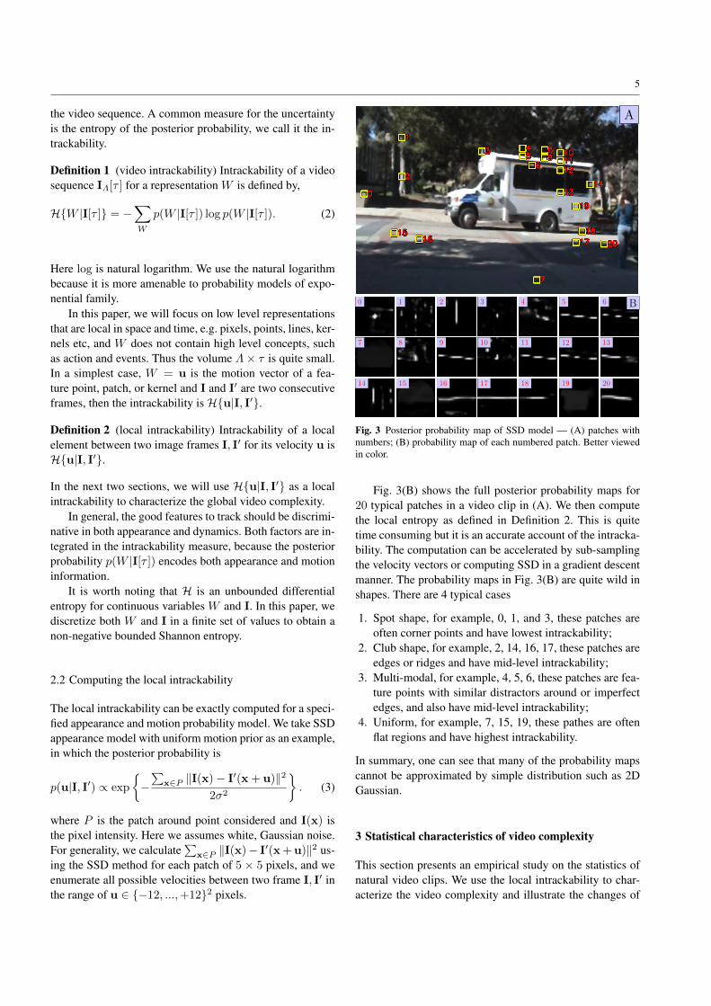
Fig. 3 Posterior probability map of SSD model — (A) patches withnumbers; (B) probability map of each numbered patch. Better viewedin color.

Fig. 3(B) shows the full posterior probability maps for20 typical patches in a video clip in (A). We then computethe local entropy as defined in Definition 2. This is quitetime consuming but it is an accurate account of the intracka-bility. The computation can be accelerated by sub-samplingthe velocity vectors or computing SSD in a gradient descentmanner. The probability maps in Fig. 3(B) are quite wild inshapes. There are 4 typical cases

1. Spot shape, for example, 0, 1, and 3, these patches areoften corner points and have lowest intrackability;

2. Club shape, for example, 2, 14, 16, 17, these patches areedges or ridges and have mid-level intrackability;

3. Multi-modal, for example, 4, 5, 6, these patches are fea-ture points with similar distractors around or imperfectedges, and also have mid-level intrackability;

4. Uniform, for example, 7, 15, 19, these pathes are oftenflat regions and have highest intrackability.

In summary, one can see that many of the probability mapscannot be approximated by simple distribution such as 2DGaussian.

3 Statistical characteristics of video complexity

This section presents an empirical study on the statistics ofnatural video clips. We use the local intrackability to char-acterize the video complexity and illustrate the changes of

6

representations over two main axes of changes. Our objec-tive is to gain some insights regarding the various regimesof motion patterns.

3.1 Histograms of local intrackability

As the local intrackability is computed in a local space-timevolume, we collect the histogram of the intrackabilities bypooling them over the image latticeΛ, following the study ofnatural image statistics where people collected histogramsof local filtered responses.

In our first experiment, we collect a set of 202 videoclips of birds from various websites, such as National Ge-ography and Flickr. Each clip has 6 frames and is resized tothe same size (176 × 144) so that the intrackability is com-puted in the same range. The reason why we choose birdvideos is that birds are captured in a wide range of scales(distance), density, and motion dynamics against clean skyor water. They are ideal for studying the change of repre-sentations. As we set u in the range of {−12, ...,+12}2, themaximum value of intrackability is log(23 × 23) ≈ 6. Weselect 60 bins for the histogram of the local intrackabilityand thus treat it as a 60-element vector. To better calculatethe distance (i.e., Bhattacharyya distance (Comaniciu et al,2003)) between histograms, we take the square root for eachelement.

Fig. 4 shows six typical examples of the square-rootedhistograms of local intrackabilities. From our experiments,we observe that there are in general three regimes of motionpatterns in these video.

– Flat or noisy videos, such as examples 1 and 6 where thebirds are far away and very dense. The intrackability ismostly focused on the right end of the histogram.

– Structured videos, such as example 2, where the birdsare close and sparse. The intrackability histogram is widelyspread as it contains elements that are trackable (e.g. thecorners of bird shapes) and elements that are intrackable(flat patches inside and outside the birds).

– Textured video, such as example 4, where the birds aredense but distinguishable from each other. The birds gen-erate texture images of middle granularity.

As we zoom-out from example 4 to examples 3, 5, and 6,we gradually observe a clear migration from the low intrack-ability bins to the high intrackability bins, finally it will endup like example 1. Row 3 of Fig. 4 verifies our intuitive ob-servation. We conduct a PCA analysis over the 202 square-rooted histograms. The mean histogram has two peaks attwo ends, therefore, we tried to use a mixture of two distribu-tions p0(h) = λ0 exp(λ0h) and p1(h) = λ1 exp(λ1(hmax−h)), where hmax is the last bin of the histogram. However,we found that it is not enough to cover the middle part.Thus, we introduce one more Gaussian. Therefore, the mean

histogram can be fitted with three mixed sub-distributions.The two eigen-vectors clearly identify the two major transi-tions. The first eigen-vector shows the change between thetrackable (textured or structured) and the intrackable (flator noise), reflecting the increasing complexity. The secondeigen-vector shows the change between the highly trackableand the less trackable, reflecting the change of granularity inscaling.

For comparison, we use Shi-Tomasi texturedness mea-sure and Harris-Stephen R score to do the same PCA. Theresults are shown in Fig. 6 and 7 respectively. Shi-Tomasiis a local measure that only accounts for the gradient infor-mation in the patch, and does not take into account similarobjects around. Therefore, it takes videos of dense small ob-jects as trackable, and puts them on the left side of Fig. 6. Inthe results of Harris-Stephen (Fig. 7), the structural videosare concentrated in a small region near the right side.

3.2 Scatter plot and variation directions

In our second experiment, we visualize the two types of tran-sitions observed in the previous step. We embed the 202

bird videos in the two dimensions spanned by the two eigen-vectors, and show the result in Fig. 5. We collect the videoson the boundary of the scatter plot and find the two curvesrepresenting the two major changes between the most in-trackable videos (flat videos on the upper-left corner) andthe most trackable (large grained textures on the upper-rightcorner). We call the flat videos intrackable and large grainedtextures as trackable, this conflicts with intuition that the flatones are easier to track. More precisely, the upper-left videosinclude objects that are easier to track, but the videos them-selves are not. Before we select which elements to track,we have no idea of objects (suppose we do not have back-ground modeling or object detection). If we try to track allthe elements in a video, the intrackabilities of blank areasare higher because of the aperture problems. We need to re-move the blank regions, which are both difficult to track andmeaningless in most cases. This is the motivation of repre-sentation pursuit in Section 4.

Why is this interesting? Traditional vision research onvideo has been studied in two separate domains: (i) track-able motion including motion flow analysis and object track-ing, and (ii) intrackable motion or textured motion. Our ex-periment shows, perhaps the first time in the literature, thatthere is a continuous transition between the two domains.Furthermore this transition occurs along two axes. The bot-tom of Fig. 5 visualizes some videos along the two curves.The first row displays videos along the upper boundary ofthe plot and reflects the change of bird density. The secondrow displays videos along the lower boundary and reflectsthe change of bird granularity through scaling. The videosin the interior of the plot in Fig. 5 contain birds of different

7

Fig. 4 (Row 1-2) Six examples of the square-rooted histograms of local intrackabilities. (Row 3) Three components are fit to the mean histogram,and the first two eigen-vectors of these square-rooted histograms reveals the transitions betweem the three components.

sizes and numbers and therefore are mixed video of the oneon the boundary. Such observations call for a unified frame-work for modeling all video patterns and for a continuoustransition between the various motion representations.

As the two curves form a loop of two continuous changes,we re-organize the videos on the boundary and visualizethem in Fig. 8.

For tracking tasks, we are interested in trackable ele-ments in a video and most intrackable areas are discardedto reduce computing burden. We apply a threshold (1/3 ofthe maximal intrackability value) on each video to obtain aset of trackable elements, and the sum of the intrackabili-ties of all trackable elements in a video provides the uncer-tainty of the tracking task. Fig. 9 plots the total sum of theintrackabilities in these trackable areas for all the videos onthe blue curve and red curve in Fig. 5. This figure illustratesthat the sum achieves the peak at populous videos, whichmeans that they are the most difficult to track when we have

Fig. 9 Total intrackability in trackable area for each video on theboundary, the red and blue curves correspond those in Fig. 5.

given up the intrackable uniform region and textured regionwith high intrackabilities. For videos with modest numberof objects, each feature point has less ambiguity. For flat or

8

Complexity increasing

Text

ure

to S

truct

ure

Fig. 5 PCA embedding of histograms of intrackabilities for the 202 bird videos in two dimensions. Red and blue curves show two typicaltransitions: The blue curve (top) shows density changes of elements (objects) in the video: from a few birds to thousands of birds. The red curve(bottom) shows scales changes in the videos: from fine granularity to large granularity. In the bottom, the first row shows the video examples onthe blue curve and the second row shows the video examples on the red curve.

noisy videos, the number of trackable points is almost zero,so the tracking algorithm can do nothing. Therefore, it hasto switch to appearance models, such as the spatio-temporalauto-regression (STAR) model, to represent the video ap-pearance without explicitly computing the motion. In thissense, the intrackability is indeed a good measure for thetransition of models.

In our third experiment, we extend the study of bird videoto general natural video clips in the same way. We collecteda set of 237 video clips containing a large variety of objects,such as people, birds, animals, grasses, trees, water with dif-ferent speed and density in natural environments. Fig. 10shows the results of the two-dimensional embedding.

The result coincide with the bird experiments. The 237

video clips are bounded by the two typical transition curves.The bottom of Fig. 10 shows the typical video clips alongthe two curves.

4 Pursuing hybrid video representations

In this section, we study a method for automatically select-ing the optimal video representations based on an intracka-bility measure. We start with an overview of some popularrepresentations in four different regimes.

9

Fig. 6 PCA embedding of histograms of Shi-Tomasi texturedness measure for the 202 bird videos in two dimensions. Red and blue curves showtwo typical transitions in Fig. 5.

4.1 Overview of four video representations

We have discussed the four distinct representations in Fig. 1:contour, kernel or PCA Basis, dense motion field, and jointimage appearance model. We divide them into two cate-gories. For the first three types of representations, there area number of elements to track, so we call them the trackablemotion. We denote the appearance and geometry of these el-ements by a dictionary ∆ = {ψ1, ..., ψn} and their motionvelocity by W = (u1, ...,un). For the fourth representa-tion, there is nothing to track and thus W does not containvelocity variables and only has some parameters. We call itintrackable motion.

Trackable motion For the contour, kernel, PCA basis,and dense motion, the posterior probability is

p(W |I, I′;∆) ∝ p(u1, · · · ,un)n∏i=1

p(IΛi|ui, I′;ψi) (4)

In the above formula, p(IΛi|ui, I′;ψi) is the local likelihood

probability for tracking an element ψi in a patch (domain)Λi discussed before,

p(IΛi|ui, I′;ψi) ∝ exp

{−∑

x∈Pi‖I(x)− I′(x+ ui)‖2

2σ2

}

which is consistent with Eq. 3 if we assume a uniform mo-tion prior. For clarity and generality, we use the SSD mea-sure based on the image patch I(x) and I′(x + ui) for x ∈Pi, this could be replaced by other features defined on ψi(x)and ψ′i(x+ u).

The joint probability p(u1, · · · ,un) is a contextual modelfor the coupling of these moving elements.

– In contour tracking (Maccormick and Blake, 2000; Satoand Aggarwal, 2004; Black and Fleet, 2000), all the pointsmay show a rigid affine transform plus some local smalldeformations. Furthermore the velocity ui = (u⊥i , u

‖i )

10

Fig. 7 PCA embedding of histograms of Harris-Stephen R score for the 202 bird videos in two dimensions. Red and blue curves show two typicaltransitions in Fig. 5.

Increase number of objects

Decrease granularity of texture

Fig. 8 The continuous change between different videos through two major axes:the change of density and the change of granularity.

11

Complexity increasing

Text

ure

to S

truct

ure

Fig. 10 PCA embedding of histograms of intrackabilities for the 237 natural videos in two dimensions. Red and blue curves show two typicaltransitions: The blue curve (top) shows density changes of elements (objects) in the video. The red curve (bottom) shows scales changes in thevideos: from fine granularity to large granularity. In the bottom, the first row shows the video examples on the blue curve and the second row showsthe video examples on the red curve.

is reduced to u⊥i containing only the direction perpen-dicular to the contour. The tangent speed is discarded asit cannot be inferred reliably (due to high entropy). Theelement ψi could be the patch or image profile along thenormal direction of the contour at key points.

– In kernel tracking (Comaniciu et al, 2003; Collins, 2003),all the interior feature points are assumed to have thesame velocity (rigid) or adjacent points are assumed tohave similar velocity. The element ψi could be the fea-ture descriptor like SIFT or PCA basis.

– In the dense motion field, (u1, · · · ,un) is regulated bya Markov random field (Horn and Schunck, 1981; Blackand Fleet, 2000). The elements ψi is either a pixel or afeature point.

These models p(u1, · · · ,un) essentially reduce the random-ness of the motion or equivalently the degrees of freedom inW . In the next subsection, we will pursue such representa-tions by reducing the variables in W .

Intrackable motion When the motion includes a largenumber of indistinguishable elements, it is called dynamictexture (Szummer and Picard, 1996; Fitzgibbon, 2001; Soattoet al, 2001) or textured motion (Wang and Zhu, 2003), suchas fire flame, water flow, evaporating steam etc. As the mov-ing elements are indistinguishable, the velocity cannot beinferred meaningfully and W is empty. These videos arerepresented by appearance models directly, typically by re-gression models. An example is the spatio-temporal auto-

12

(b) Point intrackability map

(c) Line intrackability map

(a) Input video

(d) Tri-map

IntrackabilityScore S(W)

(f) hybrid representation W*

(e)

Fig. 11 Pursuing a hybrid video representation. From an input video (a), we compute the intrackability map (b) and projected line intrackabilitymap (c) where darker point has lower intrackability. Then trimap (d) visualizes the three different representations: red spots are trackable andrepresented by key points or kernels; green areas are trackable after projecting to line segments and therefore are represented by contours, and theblack area is intrackable motion and is represented by STAR model. We plot the intrackability H(W )|I, I′ and S(W ) in (e) where the horizontalaxis is the number of variables in W from simple to complex. The optimal representation W ∗ (f) corresponds to the minimum score S(W ) shownby the star point on the curve in (e).

regression (STAR) model,

I(x, t) =∑

(y,s)∈∂(x,t)

αy−x,s−tI(y, s) + n(x, t), ∀x, t. (5)

That is, the pixel intensity at x and frame t is a regression ofother pixels in the spatio-temporal neighborhood (∂(x, t))plus some residual noise n(x, t). The model is representedby some parameters Θ = (αy−x,s−t) which are often ho-mogeneous in space and time. These parameters are learnedby fitting certain statistics. The spatio-temporal neighbor-hood may be selected for different videos. In general, onecan rewrite the video IΛ[0, T ] in a Gaussian Markov randomfield model,

p(IΛ[0, T ];Θ) ∝ exp

{−∑Tt=1

∑x∈Λ n

2(x, t)

2σ2o

}. (6)

4.2 Automatic selection of hybrid representations

A natural video often includes multiple objects or regions ofdifferent scales and complexities and thus is best representedby a hybrid representation. Fig. 11 shows an example. Thebird in the foreground is imaged at a near distance. Somespots (the head, the neck, the leg, and the end of the wings)are distinguishable from the surrounding areas and there-fore their intrackability is low as shown in (b). They shouldbe represented by key points or kernels that can be trackedover a number of frames. The points along the bird outlineare less trackable and have higher intrackability value in (b).But after projecting to line segments through merging ad-jacent points and dropping the tangent directions from W ,

these line segments become trackable. Fig. 11(c) shows theintrackability map of the lines. For the remaining areas, thewavy water in the background is textured motion and theinterior of the bird is flat area are intrackable and thus arerepresented by STAR (or MRF) models. The so-called tri-map in (d) illustrates the three different regimes of modelscalculated according to their intrackabilities. This represen-tation will have to change as the bird fly near or away fromthe camera, or the number of birds changes as many othervideos have shown in the previous section.

Automated selection and on-line adaptation of such hy-brid representations is of practical values for both computerand biologic visual systems. Given the limited resources (mem-ory and computing capacity), the system must perform atrade-off between more detail and less intrackability wisely.Psychological experiments show that human vision changesthe task and perception as well when the complexity exceedsthe system capacity (Pylyshyn, 2004, 2006).

The criterion that we use for selecting the hybrid repre-sentation W ∗ includes two objectives:

– The representation should be as detailed as possible sothat it does not miss important motion information. Thisencourages representation with high complexity.

– The representation should be inferred reliably. In otherwords, it has a lower uncertainty or entropy.

The two objectives are summarized into the following func-tion,

S(W ) = H{W |IΛ[t, t+ τ ]} −A(W ). (7)

We assume W is fixed in a short duration τ ,H{W |IΛ[t, t+τ ]} is the instance intrackability defined before, and A(W )

13

is the description (coding) length for the variables in W . Weminimize the criterion S(W ) to obtain the best representa-tion, W ∗ = argminW S(W ).

Fig. 11(e) gives an example of the criterion S(W ) againstthe number of variables in W . By minimizing this function,we obtain a representation W ∗ which is shown in Fig. 11(f).It consists of a number of trackable points, lines, contoursand intrackable regions.

MAP is a popular method for video representation, e.g.,(Wang et al, 2005; Wang and Zhu, 2008). Video representa-tion can be decomposed into two sub problems, 1) choosingvariables and 2) estimating the values of the selected vari-ables. The MAP work in fact treats both of them in a singlecriterion. In this paper, we encourage separate investigationof the two and focus on the first problem, which is more im-portant. Our answer to the first one is to select what are goodfor the second problem. After the first one is determined, theestimation of the values can be accomplished by MAP, ex-pectation or sampling.

In the following, we introduce the representation projec-tion operators that compute W ∗ and realize the transitionbetween the models.

4.3 Representation projection

We start with an overly detailed representationWo = (u1, ...,uN )

with N be the number of points that densely sampled in theimage lattice. The motion velocity ui, i = 1, 2, ..., N are as-sumed to be independent in the range of [−12, 12]2 pixels.Therefore we have

S(Wo) =

N∑i=1

H{ui|I, I′} − λ · 2N,

where λ is the description length of each velocity direction.Wo is the most complex representation corresponding to theright end of the plot in Fig. 11(e). We convert it to a hybridrepresentation W ∗ by representation projection with fourtypes of operators. Each operator will reduce S(Wo) in agreedy way (i.e. pursuit).

1. Point dropping. We may drop the highly intrackablepoints (or image patches). By dropping an element ui fromW , the change of S(W ) is

∆i = −H{ui|I, I′}+ 2λ < 0.

In other words, any point with H{ui|I, I′} < 2λ remainsin W as a “trackable points” which are indicated by the redcrosses in Fig. 11(f). We also perform a non-local-maximumsuppression. Because our local intrackability is estimatedbased on patches (say 11×11 pixels), thus any points withina neighborhood (say 5 × 5) of the trackable points will besuppressed.

2. Velocity projection. For the remaining points, we projectthe velocity u to one dimension u⊥ so that the projected ve-locity has the lowest intrackability,

H{u⊥|I, I′} = minξH{〈ξ,u〉|I, I′}

in which ξ is a unit vector representing the selected orien-tation. If the patch contains an edge, the most likely orien-tation ξ is the normal direction of the edge. Fig. 11(c) illus-trates the projected intrackability. If we let u′ be the compo-nent of u that is perpendicular to u⊥, that is u = (u⊥, u

′).Then we have

H{u|I, I′} = H{(u⊥, u′)|I, I′} (8)

= H{u⊥|I, I′}+H{u′|u⊥, I, I′} (9)

in which H{u′|u⊥, I, I′} is the conditional entropy of u′

given u⊥, and is always non-negative. Therefore we have

Proposition 1 Intrackability decreases with representationprojection, i.e.,H{u⊥|I, I′ } 6 H{u|I, I′}.

While u is intrackable, its component u⊥ may still be track-able along the normal direction. Thus, we replace the ele-ment ui by u⊥ in W . This leads to a change of S(W ):

∆i = H{ui|I, I′} −H{u⊥|I, I′ }+ λ < 0.

In other words, we drop the direction which has large en-tropy.

Fig. 11(d) shows the tri-map in dense point where a redpoint is trackable, a green point is trackable in a projecteddirection, and a black point is intrackable. Fig. 12 shows thetrimaps for four examples with different choices of thresh-olds.

3. Pair linkage. After eliminating the points in the pre-vious two steps, we further reduce S(W ) by exploring thedependency between the elements. We sequentially link ad-jacent points or lines into a chain structure (contours). Sup-pose the resulting contour has k points/lines (u1,u2, ...,uk),we assume these elements follow a Markov chain, so

p(u1,u2, ...,uk|I, I′) = p(u1|I, I′)k∏i=2

p(ui|ui−1, I, I′).

Proposition 2 Pair linking reduces the intrackability

H{u1, ...,uk|I, I} =k∑i=1

H{ui|I, I′} −k∑i=2

M(ui,ui−1|I, I′)

6k∑i=1

H{ui|I, I′}, (10)

whereM(ui,ui−1|I, I′) > 0 is the conditional mutual in-formation between two adjacent elements.

14

Hybrid representations

Trimaps

Example 1:contour

Hybrid representations

Trimaps

Example 2:kernels

Hybrid representations

Trimaps

Example 3:

Hybrid representations

Trimaps

Example 4:

motion flow

appearance

Fig. 12 Trimaps and pursued hybrid representations at different thresholds: red — trackable points, green — trackable lines in projected direction,black — intrackable points. For each video, from left to right, threshold varies from high to low. The first video can be best represented by contours.The second video can be best represented by kernels. The third video can be best represented by dense points. The forth can be best representedby appearance models.

15

Fig. 13 More results of hybrid representation pursuit in 12 video clips. In each example, we show the hybrid representations: red crosses aretrackable points, red ellipses are grouped kernels; and green curves are the trackable contours. In the background, we show the score curves S(W )

in black and the intrackability curve in red. The asters on the black curves indicate the minima. The horizontal axis is the number of variables inW . The vertical axis is the intrackability or the score.

16

The mutual information is defined as

M(ui,ui−1|I, I′) (11)

=∑

ui,ui−1

p(ui,ui−1|I, I′) logp(ui,ui−1|I, I′)

p(ui|I, I′)p(ui−1|I, I′)(12)

= H{ui|I, I′} −H{ui|ui−1, I, I′} (13)

Eq. (12) shows that it is Kullback-Leibler divergence fromp(ui,ui−1|I, I′) to p(ui|I, I′)p(ui−1|I, I′), and therefore non-negative.

In S(W ), the reduction of the intrackability is the mu-tual information at each step, the number of variablesA(W )

remains the same, though we may need to index the chainstructure with a coding length of ε. So each time by linkinga pair of elements ui, we have a change of S(W ) by

∆i = −M(ui,ui−1|I, I′) + ε < 0. (14)

We computeM(ui,ui−1|I, I′) by Eq. (13). To compute theconditional entropy H{ui|ui−1, I, I′}, one may enumerateall possible combinations of (ui,ui−1), then compute theconditional probability, joint probability and entropy. As afaster approximation, we find the optimal solution u∗i−1 first,and then computeH{ui|u∗i−1, I, I′}. T-junctions can be foundautomatically when we greedily grow the set of projectedtrackable element by pair linking.

4. Collective grouping. This operator is to group a num-ber of adjacent elements in an ellipse simultaneously into akernel representing a moving object. Given the velocity u0

of the kernel, the grouped elements u1, ...,uk are assumedto be conditionally independent,

p(u0,u1,u2, ...,uk|I, I′) = p(u0|I, I′)k∏i=2

p(ui|u0, I, I′).

Therefore the change of S(W ) is

∆1..k = H{u0|I, I′} −k∑i=1

M(ui,u0|I, I′) < 0

In practice, we place an ellipse around each trackable pointin the trimap, and if there are a few trackable points, forwhich the best estimations of velocities are very close, thenwe group them into a kernel.

4.4 Experiment on pursuing hybrid representation

The precise optimization of S(W ) is computationally in-tensive, so we use a greedy algorithm which starts with thedense point representation Wo, then sequentially apply thefour operators to reduce S(W ). The final result is a hybridrepresentation consisting of: trackable points (red crosses),trackable lines (green), contours (green), kernels (red ellipses),and the remaining intrackable regions.

In addition to the results in Fig. 11 and 12, we tested thepursuit algorithm on a variety of video clips. Fig. 13 shows12 examples representing videos of different complexities.In row 1: the foreground objects (bird, human, and fish) ex-hibit high resolution in a flat background. The contours andshort lines dominate the representation. In row 2: the objects(birds, fish, and people) exhibit low resolution and are wellseparated from the background. Thus, they are representedby kernels. In row 3, the objects (still people, fish, birds)exhibit low resolution and high density. As many elementsare still distinguishable in their neighborhood, they are rep-resented by dense trackable points. In row 4, there are notrackable elements, the video becomes a texture appearanceand thus described by STAR model.

From the final pursuit results, one can see that most ofthe feature points and the object contours are captured suc-cessfully. The junctions on car (especially the window cor-ner) and person (cloth corners) are well classified as sparsefeature points, and the edges and contours are well classi-fied as lines. The horizontal line between the water and sandin the first row is not selected as trackable line due to weakedge contrasts and similar lines in their neighborhood.

Fig. 14 shows additional results on two longer sequences.The top row shows a swimming shark represented by con-tour and feature points. The bottom row shows a movingcamera approaching a car. At first, the car is very far away,and appears as a feature point. As the camera approaches,it is represented by a kernel. As the camera approaches fur-ther, more details are revealed, and it is represented by a setof contours, kernels and feature points.

5 Comparison with other tracking criteria

In this section, we compare the intrackability with two othermeasures for robust tracking, namely the Shi-Tomasi tex-turedness measure and the conditional number.

5.1 Intrackability and the texturedness measure

(Shi and Tomasi, 1994) proposed a texturedness criterion forgood points to track in two frames. To compare with this cri-terion, we rewrite the local posterior probability for a pointvelocity u = (ux, uy) that we discussed before,

p(u|I, I′) ∝ exp

{−∑

x∈P |I(x)− I′(x+ u)|2

2σ2

}.

As it is common in optical flow computation, one assumesthe image is differential with (Ix, Iy) being the image gra-dient. By Taylor expansion we have

I′(x+ u) = I(x) + uxIx + uyIy. (15)

17

30 60 80 113 170

20 40 90 105 109

Fig. 14 Experiments on longer sequences.

Intra

ckab

ility

Shi-T

omas

i

Frame 0

Frame 20

Frame 0

Frame 20

Frame 0

Frame 13

Frame 13

Frame 0 Frame 0

Frame 17

Frame 17

Frame 0

Fig. 15 Tracking comparison: In the first column, the intrackability measure tracks slightly better than Shi-Tomasi measure. In the second andthird columns, the intrackability measure can distinguish subtle trackable points from the clothes, but Shi-Tomasi measure selects more repetitivefeature points and makes more mismatches across frames.

18

Then we can rewrite p(u|I, I′) in a Gaussian form,

p(u|I, I′) = 1

2πdet1/2(Σ)exp{−1

2uΣ−1u′}. (16)

where the inversed covariance matrix is,

Σ−1 =

(∑x∈P I2x(x)

∑x∈P Ix(x)Iy(x)∑

x∈P Ix(x)Iy(x)∑

x∈P I2y(x)

)(17)

Let λmax ≥ λmin be the two eigen-values of Σ−1, then thelocal intrackability is

H{u|I, I′} = log 2π +1

2det(Σ),

= log 2π − 1

2log λmaxλmin.

Therefore, large eigen-values leads to lower intrackabilityand thus to better points to track. In the projected directionu⊥, we drop the dimension that has lower eigen-value, andthe intrackability of a oriented line is

H{u⊥|I, I′} =1

2log 2π − 1

2log λmax

In comparison, (Shi and Tomasi, 1994) used λmin as a tex-turedness measure. Larger λmin means higher intensity con-trast in the patch and thus a better point to track.

We can see that the differences between intrackabilityand the Shi-Tomasi measure are

1. Shi-Tomasi uses Taylor expansion as an approximationof local image patch. This assumes that the image is con-tinuous and may be violated at the boundary or in tex-tured motion.

2. λmin is used instead of log λmaxλmin measure.

It is worth to note that this texturedness measure is mosteffective in a video regime corresponding to the rightmostextreme in Fig. 5 (bird flock) and Fig. 10 (marathon) wherethe objects are dense and still distinguishable from the sur-roundings. In our pursued hybrid representations, most track-able points are selected in this regime in Fig. 13 (row 3).

We compare with (Shi and Tomasi, 1994) in selectinggood features to track in frame-to-frame tracking. The Shi-Tomasi criterion measures texturedness in a single imagepatch of 5 × 5 pixels, in contrast our intrackability is com-puted between frames in a [−12, 12]2 displacement rangeand thus is searched in a larger neighborhood. As Fig. 15illustrates, we manually initialize a polygon region for theobject of interest, then trackable points are pursued in theregion and tracked across frames by finding the best SSDmatches. After point-wise matching, an affine transforma-tion is fitted to obtain the current polygon of object region.For an object with no self-similar feature, our results is sim-ilar to or slightly better than the Shi-Tomasi measure, seethe first column in Fig. 15. But for objects with many self-similar features, the Shi-Tomasi measure will be misguided

to hit these self-similar ones, which often results in mis-matches between frames. In Figure 15, the second and thirdcolumn show that the intrackability measures can distinguishthe more informative points on collars, shoulders, buttonsand pockets in most places, but Shi-Tomasi measures failsto do so in more places.

To make quantitative comparison of the performances,we annotate the ground truth of the vertices of outer poly-gons for the three sequences in Fig. 15 and measure the av-erage errors of all vertices over time. Let xi,t be the groundtruth of the position of the i-th vertex in frame t, x̂i,t be itsestimated value by a tracking algorithm, M be the numberof vertices, the tracking error of frame t is defined as

Errort =1

M

∑i

‖xi,t − x̂i,t‖ (18)

The resultant error curves are shown in Fig. 16.Harris-Stephens R score (Harris and Stephens, 1988) is

also based on the matrix in Eq. (17). It is defined as R =

det(Σ−1) − ktrace(Σ−1)2, which is equivalent to R =

λmin ∗λmax− k(λmin +λmax)2, where k is a small weight.

It is clear that our intrackability measure log(λmin ∗ λmax)

is the log of an upper bound to R score.

5.2 Intrackability and the condition number

(Fan et al, 2006) proposed to use the conditional number of amatrix as an uncertainty measure in tracking a kernel. Unlikepoint tracking, a kernel tracking uses a histogram feature ina larger scope. Let h0 be the histogram as a model of thetarget. In the next frame, mean-shift is used to find the opti-mal motion vector u of the target, starting from a predictedposition. Let h1 be the histogram at the predicted position,Fan et al (Fan et al, 2006) began with the linearized kerneltracking equation system

Mu =√

h0 −√h1 (19)

where M = (d1, · · · ,dm)T is a matrix composed of cen-

ters of mass of all color bins and dj is the j-th mass cen-ter. Let A = MTM be the matrix with two eigenvaluesλmax and λmin. The condition number of A is λmax/λmin >1. Small condition number will result in stable solution toEq 19 and thus a better kernel to track.

To compare with this measure, we rewrite the local pos-terior probability for the velocity u according to this setup,

p(u|h0,h1) ∝ exp

{−‖Mu− (

√h0 −

√h1)‖2

tr(A)

}. (20)

where the trace tr(A) = λmax + λmin is introduced to nor-malize the histogram differences. This is also a two dimen-sional Gaussian with covariance matrix

Σ = tr(A)A−1. (21)

19

Fig. 16 Quantitative performance comparison — left is the magazine sequence (left column in Fig. 15), middle is the phone-call sequence (middlecolumn in Fig. 15), and right the cloth sequence (right column in Fig. 15).

Therefore, the local intrackability is the entropy of p(u|h0,h1).

H{u|h0,h1} =1

2+ log 2π − log

√λmaxλmin

λmax + λmin(22)

=1

2+ log 2π − log

√λmax/λmin

λmax/λmin + 1. (23)

This is a monotonically increasing function with respect tothe condition number λmax/λmin as λ1/λ2 > 1.

In light of the same derivation process, other covariancerelated measure such as those mentioned in (Zhou et al,2005) can all be regarded as an intrackability under someGaussian distribution assumption.

6 Discussion

Despite the vast literature in motion analysis, tracking, andvideo coding, the connections and transitions between vari-ous video representations have not been studied. In this pa-per, we study the intrackabilities of local image entities (points,lines, patches) as a measure of the inferential uncertainty.Using the histogram of the intrackabilities pooled over thevideo in space and time as the global video statistics, wemap natural video clips in a scatter plot and thus in differentregimes. We find two major axes in the plot representing im-age scaling and change of object density respectively. As avideo may contain multiple patterns in different regimes, wedevelop a model selection criterion based on the intrackabil-ity and model complexity to pursue a hybrid representationwhich integrate four components: trackable points, trackablelines, contours, and textured motion. This criterion guidesthe transition of representations due to image scaling andchange of object density.

In representing generic images, researchers have devel-oped sparse coding model for structured image primitives,such as edges, bars, and corners etc and texture model basedon Markov random fields for stochastic textures which donot have distinct elements. The integration of these modelshas led to a primal sketch model conjectured in (Marr et al,1979). In ongoing project, we are extending the hybrid rep-resentation to a video primal sketch model as a generic video

representation for effective coding and for modeling variousactions.

Acknowledgement

The authors would like to thank Dr. Yingnian Wu at UCLAfor discussions and thank Youdong Zhao at Lotus Hill Insti-tute for assistance. This work is supported by NSFC 60832004and 60875005.

References

Ali S, Shah M (2007) A lagrangian particle dynamics ap-proach for crowd flow segmentation and stability analy-sis. In: CVPR

Ali S, Shah M (2008) Floor fields for tracking in high den-sity crowd scenes. In: ECCV

Badrinarayanan V, Perez P, Le Clerc F, Oisel L (2007) Onuncertainties, random features and object tracking. In:ICIP

Black MJ, Fleet DJ (2000) Probabilistic detection and track-ing of motion boundaries. IJCV 38(3):231–245

Collins R, Liu Y, Leordeanu M (2005) Online selectionof discriminative tracking features. PAMI 27(10):1631–1643

Collins RT (2003) Mean-shift blob tracking through scalespace. In: CVPR

Comaniciu D, Ramesh V, Meer P (2003) Kernel-based ob-ject tracking. PAMI 25(5)

Cong Y, Gong H, Zhu SC, Tang Y (2009) Flow mosaick-ing: Real-time pedestrian counting without scene-specificlearning. pp 1093–1100

Dreschler L, Nagel HH (1981) Volumetric model and 3Dtrajectory of a moving car derived from monocular TVframe sequences of a street scene. In: IJCAI, pp 692–697

Fan Z, Yang M, Wu Y, Hua G, Yu T (2006) Effient optimalkernel placement for reliable visual tracking. In: CVPR

Fitzgibbon A (2001) Stochastic ridigity: Image registrationfor nowhere-static scenes. In: ICCV

20

Han TX, Ramesh V, Zhu Y, Huang TS (2005) On optimizingtemplate matching via performance characterization

Harris C, Stephens M (1988) A combined corner and edgedetector. In: Proceedings of The Fourth Alvey VisionConference, Manchester, UK, pp 147–151

Horn B, Schunck B (1981) Determining optical flow. Artifi-cial Intelligence 17:185–203

Kadir T, Brady M (2001) Saliency, scale and image descrip-tion. IJCV 45(2):83–105

Koenderink JJ (1984) The structure of images. BiologicalCybernetics 50:363–370

Kwon J, Lee KM, Park FC (2009) Visual tracking via geo-metric particle filtering on the affine group with optimalimportance function. IEEE Conf on Computer Vision andPattern Recognition

Li Z, Gong H, Sang N, Zhu G (2007a) Intrackability theoryand application. In: SPIE MIPPR

Li Z, Gong H, Zhu SC, Sang N (2007b) Dynamic fea-ture cascade for multiple object tracking with trackabilityanalysis. In: EMMCVPR

Lindeberg T (1993) Detecting salient blob-like image struc-tures and their scales with a scale-space primal sketch: Amethod for focus-of-attention. IJCV 11(3):283–318

Maccormick J, Blake A (2000) A probabilistic exclusionprinciple for tracking multiple objects. IJCV 39(1):57–71

Marr D, Poggio T, Ullman S (1979) Bandpass channels,zero-crossings, and early visual information processing.JOSA 69:914–916

Nickels K, Hutchinson S (2002) Estimating uncertainty inssd-based feature tracking. Image and Vision Computing20(1):47–68

Pan P, Porikli F, Schonfeld D (2009) Recurrent tracking us-ing multifold consistency. In: IEEE Workshop on VS-PETS

Pylyshyn ZW (2004) Some puzzling findings in multiple ob-ject tracking (MOT): I. tracking without keeping track ofobject identities. Visual Cognition 11(7):801–822

Pylyshyn ZW (2006) Some puzzling findings in multiple ob-ject tracking (mot): II. inhibition of moving nontargets.Visual Cognition 14(2):175–198

Pylyshyn ZW, Vidal Annan J (2006) Dynamics of target se-lection in multiple object tracking (mot). Spatial Vision19(6):485–504

Ross DA, Lim J, Lin RS, Yang MH (2008) Incrementallearning for robust visual tracking. Int’l Journal of Com-puter Vision 77:125–141

Sato K, Aggarwal JK (2004) Temporal spatio-velocity trans-form and its application to tracking and interaction. CVIU96:100–128

Segvic̀ S, Remazeilles A, Chaumette F (2006) Enhancingthe point feature tracker by adaptive modelling of the fea-ture support. In: ECCV

Serby D, Koller-Meier S, Gool LV (2004) Probabilistic ob-ject tracking using multiple features. In: ICPR, pp 184–187

Shi J, Tomasi C (1994) Good features to track. In: CVPRSoatto S, Doretto G, Wu Y (2001) Dynamic textures. In:

ICCVSrivastava A, Lee A, Simoncelli E, Zhu S (2003) On ad-

vances in statistical modeling of natural images. J of MathImaging and Vision 18(1):17–33

Szummer M, Picard RW (1996) Temporal texture modeling.In: ICIP

Tommasini T, Fusiello A, Trucco E, Roberto V (1998) Mak-ing good features track better. In: CVPR

Veenman C, Reinders M, Backer E (2001) Resolving motioncorrespondence for densely moving points. PAMI 23:54–72

Wang Y, Zhu S (2008) Perceptual scale space and its appli-cations. Int’l Journal of Computer Vision 80(1):143–165

Wang Y, Zhu SC (2003) Modeling textured motion : Parti-cle, wave and sketch. In: ICCV, pp 213–220

Wang Y, Bahrami S, Zhu SC (2005) Perceptual scale spaceand its applications. In: ICCV, pp 58–65

Witkin A (1983) Scale space filtering. In: Intl Joint Conf. onAI, Kaufman, Palo Alto

Wu Y, Zhu S, Guo C (2008) From information scaling ofnatural images to regimes of statistical models. Quarterlyof Applied Mathematics 66(1):81–122

Yilmaz A, Javed O, Shah M (2006) Object tracking: A sur-vey. ACM Computing Survey 38(4):13

Zhou XS, Comaniciu D, Gupta A (2005) An informa-tion fusion framework for robust shape tracking. PAMI27(1):115–123