intro to the lifecontingencies r package · pdf fileintro to the lifecontingencies r package...

Intro to the lifecontingencies R package

Giorgio Alfredo Spedicato, Ph.D C.Stat ACAS

09 dicembre, 2017

Giorgio Alfredo Spedicato, Ph.D C.Stat ACAS Intro to the lifecontingencies R package 09 dicembre, 2017 1 / 46

Intro

The lifecontingencies package (Spedicato 2013) will be introduced.As first half 2017 it is the first R (Team 2012) package mergingdemographic and financial mathematics function in order to performactuarial evaluation of life contingent insurances (annuities, lifeinsurances, endowments, etc).The applied examples will shown: how to load the R package, how toperform basic financial mathematics and demographic calculations,how to price and reserve financial products.


The final example will show how to mix lifecontingencies anddemography (Rob J Hyndman et al. 2011) function to assess themortality development impact on annuities.The interested readers are suggested to look to the package’s vignettes(also appeared in the Journal of Statistical Sofware) for a broaderoverview. (Dickson, Hardy, and Waters 2009; and Mazzoleni 2000)provide and introduction of Actuarial Mathematics theory.Also (Charpentier 2012) and (Charpentier 2014) discuss the software.


Loading the package

The package is loaded using

library(lifecontingencies) #load the package

It requires a recent version of R (>=3.0) and the markovchain package(Spedicato, Giorgio Alfredo 2015). The development version of thepackage requires also Rcpp package (Eddelbuettel 2013).


Package’s Financial Mathematics Functions


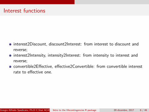
Interest functions

interest2Discount, discount2Interest: from interest to discount andreverse;interest2Intensity, intensity2Interest: from intensity to interest andreverse;convertible2Effective, effective2Convertible: from convertible interestrate to effective one.


(1 + i) =(1 + i(m)

m

)m= eδ

eδ =(1− d(m)

m

)−m= (1− d)−1


#interest and discount ratesinterest2Discount(i=0.03)

## [1] 0.02912621

discount2Interest(interest2Discount(i=0.03))

## [1] 0.03

#convertible and effective interest ratesconvertible2Effective(i=0.10,k=4)

## [1] 0.1038129


Annuities and future values

annuity: present value (PV) of an annuity;accumulatedValue: future value of constant cash flows;decreasingAnnuity, increasingAnnuity: increasing and decreasingannuities.


an = 1−(1+i)−n

isn = an ∗ (1 + i)n = (1+i)n−1

ian = an ∗ (1 + i)


annuity(i=0.05,n=5) #due

## [1] 4.329477

annuity(i=0.05,n=5,m=1) #immediate

## [1] 4.123311

annuity(i=0.05,n=5,k=12) #due, with

## [1] 4.42782

# fractional payemnts


an −n∗vn

i = (Ia)n−an

i = (Da)(Ian) + (Dan) = (n + 1) ∗ an


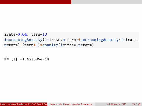
irate=0.04; term=10increasingAnnuity(i=irate,n=term)+decreasingAnnuity(i=irate,n=term)-(term+1)*annuity(i=irate,n=term)

## [1] -1.421085e-14


Other functions

presentValue: PV of possible varying CFs.duration, convexity: calculate duration and convexity of any stream ofCFs.


PV =∑

t∈T CFt ∗ (1 + it)−t

D = 1P(0)

∑Tt=τ t ct

(1+r)t

C = 1P(1+r)2

∑ni=1

ti (ti +1)Fi(1+r)ti


#bond analysisirate=0.03cfs=c(10,10,10,100)times=1:4#compute PV, Duration and ConvexitypresentValue(cashFlows = cfs,timeIds = times,interestRates = irate)

## [1] 117.1348

duration(cashFlows = cfs,timeIds = times, i = irate)

## [1] 3.409976

convexity(cashFlows = cfs,timeIds = times, i = irate)

## [1] 15.79457Giorgio Alfredo Spedicato, Ph.D C.Stat ACAS Intro to the lifecontingencies R package 09 dicembre, 2017 16 / 46

Intro

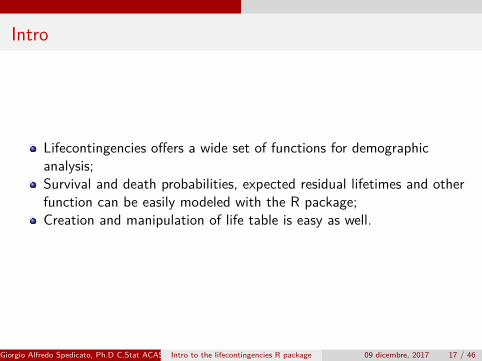
Lifecontingencies offers a wide set of functions for demographicanalysis;Survival and death probabilities, expected residual lifetimes and otherfunction can be easily modeled with the R package;Creation and manipulation of life table is easy as well.


Package’s demographic functions


Table creation and manipulation

new lifetable or actuarialtable methods.print, plot show methods.probs2lifetable function to create tables from probabilities


{l0, l1, l2, . . . , lω}Lx = lx +lx+1

2qx ,t = dx+t

lx


data("demoIta")sim92<-new("lifetable",x=demoIta$X,

lx=demoIta$SIM92, name='SIM92')getOmega(sim92)

## [1] 108

tail(sim92)

## x lx## 104 103 47## 105 104 24## 106 105 11## 107 106 5## 108 107 2## 109 108 1


Life tables’ functions

dxt, deaths between age x and x + t, tdxpxt, survival probability between age x and x + t, tpxpxyzt, survival probability for two (or more) lives, tpxyqxt, death probability between age x and x + t, tqxqxyzt, death probability for two (or more) lives, tqxyTxt, number of person-years lived after exact age x, tTxmxt, central death rate, tmxexn, expected lifetime between age x and age x + n, nexexyz, n-year curtate lifetime of the joint-life status


px ,t = 1− qx ,t = lx+tlx

ex ,n =∑n

t=1 px ,t


#two years death rateqxt(sim92, x=65,2)

## [1] 0.04570079

#expected residual lifetime between x and x+nexn(sim92, x=25,n = 40)

## [1] 37.86183


Simulation

rLife, sample from the time until death distribution underlying a lifetablerLifexyz, sample from the time until death distribution underlying twoor more lives


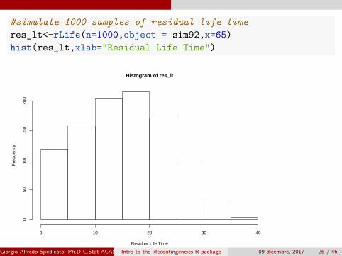
#simulate 1000 samples of residual life timeres_lt<-rLife(n=1000,object = sim92,x=65)hist(res_lt,xlab="Residual Life Time")

Histogram of res_lt

Residual Life Time

Fre

quen

cy

0 10 20 30 40

050

100

150

200


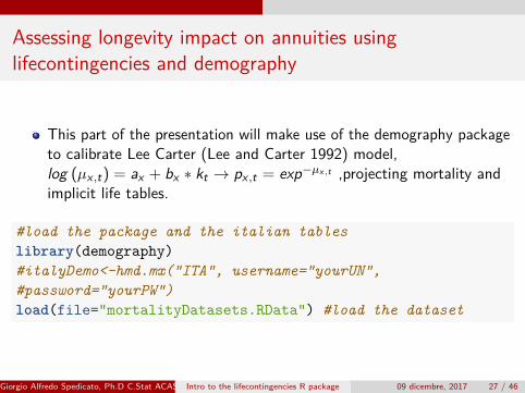
Assessing longevity impact on annuities usinglifecontingencies and demography

This part of the presentation will make use of the demography packageto calibrate Lee Carter (Lee and Carter 1992) model,log (µx ,t) = ax + bx ∗ kt → px ,t = exp−µx,t ,projecting mortality andimplicit life tables.

#load the package and the italian tableslibrary(demography)#italyDemo<-hmd.mx("ITA", username="yourUN",#password="yourPW")load(file="mortalityDatasets.RData") #load the dataset


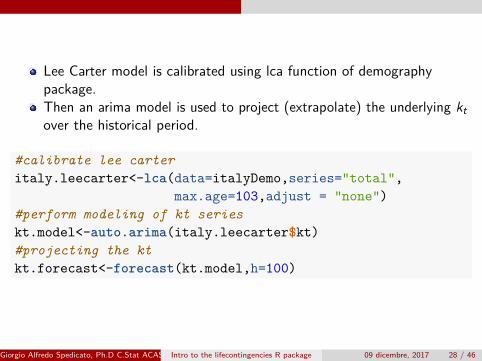
Lee Carter model is calibrated using lca function of demographypackage.Then an arima model is used to project (extrapolate) the underlying ktover the historical period.

#calibrate lee carteritaly.leecarter<-lca(data=italyDemo,series="total",

max.age=103,adjust = "none")#perform modeling of kt serieskt.model<-auto.arima(italy.leecarter$kt)#projecting the ktkt.forecast<-forecast(kt.model,h=100)


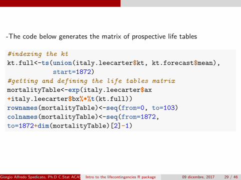
-The code below generates the matrix of prospective life tables

#indexing the ktkt.full<-ts(union(italy.leecarter$kt, kt.forecast$mean),

start=1872)#getting and defining the life tables matrixmortalityTable<-exp(italy.leecarter$ax+italy.leecarter$bx%*%t(kt.full))rownames(mortalityTable)<-seq(from=0, to=103)colnames(mortalityTable)<-seq(from=1872,to=1872+dim(mortalityTable)[2]-1)


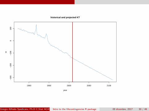
historical and projected KT

year

kt

1900 1950 2000 2050 2100

−30

0−

200

−10

00

100


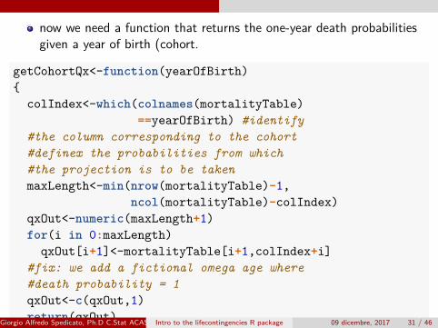
now we need a function that returns the one-year death probabilitiesgiven a year of birth (cohort.

getCohortQx<-function(yearOfBirth){

colIndex<-which(colnames(mortalityTable)==yearOfBirth) #identify

#the column corresponding to the cohort#definex the probabilities from which#the projection is to be takenmaxLength<-min(nrow(mortalityTable)-1,

ncol(mortalityTable)-colIndex)qxOut<-numeric(maxLength+1)for(i in 0:maxLength)

qxOut[i+1]<-mortalityTable[i+1,colIndex+i]#fix: we add a fictional omega age where#death probability = 1qxOut<-c(qxOut,1)return(qxOut)

}Giorgio Alfredo Spedicato, Ph.D C.Stat ACAS Intro to the lifecontingencies R package 09 dicembre, 2017 31 / 46

Now we use such function to obtain prospective life tables and toperform actuarial calculations. For example, we can compute the APVof an annuity on a workers’ retiring at 65 assuming he were born in1920, in 1950 and in 1980. We will use the interest rate of 1.5% (theone used to compute Italian Social Security annuity factors).The first step is to generate the life and actuarial tables

#generate the life tablesqx1920<-getCohortQx(yearOfBirth = 1920)lt1920<-probs2lifetable(probs=qx1920,type="qx",name="Table 1920")at1920<-new("actuarialtable",x=lt1920@x,lx=lt1920@lx,interest=0.015)qx1950<-getCohortQx(yearOfBirth = 1950)lt1950<-probs2lifetable(probs=qx1950,type="qx",name="Table 1950")at1950<-new("actuarialtable",x=lt1950@x,lx=lt1950@lx,interest=0.015)qx1980<-getCohortQx(yearOfBirth = 1980)lt1980<-probs2lifetable(probs=qx1980,type="qx",name="Table 1980")at1980<-new("actuarialtable",x=lt1980@x,lx=lt1980@lx,interest=0.015)


Now we can evaluate a65 and e65 for workers born in 1920, 1950 and1980 respectively.

cat("Results for 1920 cohort","\n")

## Results for 1920 cohort

c(exn(at1920,x=65),axn(at1920,x=65))

## [1] 16.51391 15.14127



c(exn(at1950,x=65),axn(at1950,x=65))

## [1] 18.72669 16.83391



c(exn(at1980,x=65),axn(at1980,x=65))

## [1] 20.47112 18.13948


Intro on Actuarial Mathematics Funcs

The lifecontingencies package allows to compute all classical lifecontingent insurances.Stochastic calculation varying expected lifetimes are possible as well.This makes the lifecontingencies package a nice tool to performactuarial computation at command line on life insurance tasks.


Creating actuarial tables

Actuarial tables are stored as S4 object.The lx , x , interest rate and a name are required.The print method return a classical actuarial table (commutationfunctions)


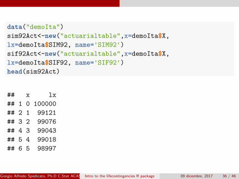
data("demoIta")sim92Act<-new("actuarialtable",x=demoIta$X,lx=demoIta$SIM92, name='SIM92')sif92Act<-new("actuarialtable",x=demoIta$X,lx=demoIta$SIF92, name='SIF92')head(sim92Act)

## x lx## 1 0 100000## 2 1 99121## 3 2 99076## 4 3 99043## 5 4 99018## 6 5 98997


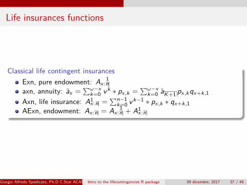
Life insurances functions

Classical life contingent insurancesExn, pure endowment: Ax :

1n

axn, annuity: ax =∑ω−x

k=0 vk ∗ px ,k =∑ω−x

k=0 aK+1 px ,kqx+k,1Axn, life insurance: A1x :n =

∑n−1k=0 vk−1 ∗ px ,k ∗ qx+k,1

AExn, endowment: Ax :n = Ax :1n + A1x :n


100000*Exn(sim92Act,x=25,n=40)

## [1] 24822.27

100000*AExn(sim92Act,x=25,n=40)

## [1] 33104.86

1000*12*axn(sim92Act,x=65,k=12)

## [1] 139696.3

100000*Axn(sim92Act,x=25,n=40)

## [1] 8282.588


Additional life contingent insurancesIncreasing and decreasing term insurances and annuities(n − 1) ∗ A1x :n = (IA)1x :n + (DA)1x :n


IAxn(sim92Act,x=40,n=10)+DAxn(sim92Act,x=40,n=10)

## [1] 0.2505473

(10+1)*Axn(sim92Act,x=40,n=10)

## [1] 0.2505473


Insurances on multiple lifesFirst survival and last survival status, both for insurances and annuitiesAxy+Axy=Ax+Ayaxy+axy=ax+ay


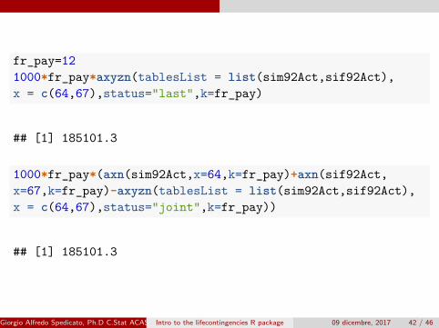
fr_pay=121000*fr_pay*axyzn(tablesList = list(sim92Act,sif92Act),x = c(64,67),status="last",k=fr_pay)

## [1] 185101.3

1000*fr_pay*(axn(sim92Act,x=64,k=fr_pay)+axn(sif92Act,x=67,k=fr_pay)-axyzn(tablesList = list(sim92Act,sif92Act),x = c(64,67),status="joint",k=fr_pay))

## [1] 185101.3


Simulation

It is possible to simulate the PV of insured benefit distributions.The rLifeContingencies function is used for single life benefit insurance.The rLifeContingenciesXyz function is used for multiple lifes benefits.


hist(rLifeContingencies(n = 1000,lifecontingency = "Axn",x = 40,object = sim92Act,getOmega(sim92Act)-40),main="Life Insurance on 40 PV distribution")

Life Insurance on 40 PV distribution

rLifeContingencies(n = 1000, lifecontingency = "Axn", x = 40, object = sim92Act, getOmega(sim92Act) − 40)

Fre

quen

cy

0.2 0.4 0.6 0.8 1.0

010

020

030

040

0


Bibliography I


Bibliography II

Charpentier, Arthur. 2012. “Actuarial Science with R 2: Life Insurance andMortality Tables.” http://freakonometrics.blog.free.fr/index.php?post/2012/04/04/Life-insurance,-with-R,-Meielisalp.———. 2014. Computational Actuarial Science. The R Series. CambridgeUniversity Press.Dickson, D.C.M., M.R. Hardy, and H.R. Waters. 2009. ActuarialMathematics for Life Contingent Risks. International Series on ActuarialScience. Cambridge University Press.Eddelbuettel, Dirk. 2013. Seamless R and C++ Integration with Rcpp.New York: Springer.Lee, R.D., and L.R. Carter. 1992. “Modeling and Forecasting U.S.Mortality.” Journal of the American Statistical Association 87 (419):659–75. doi:10.2307/2290201.Mazzoleni, P. 2000. Appunti Di Matematica Attuariale. EDUCattUniversità Cattolica.Rob J Hyndman, Heather Booth, Leonie Tickle, and John Maindonald.2011. Demography: Forecasting Mortality, Fertility, Migration andPopulation Data. http://CRAN.R-project.org/package=demography.Spedicato, Giorgio Alfredo. 2013. “The lifecontingencies Package:Performing Financial and Actuarial Mathematics Calculations in R.” Journalof Statistical Software 55 (10): 1–36. http://www.jstatsoft.org/v55/i10/.Spedicato, Giorgio Alfredo. 2015. Markovchain: Discrete Time MarkovChains Made Easy.Team, R Development Core. 2012. R: A Language and Environment forStatistical Computing. Vienna, Austria: R Foundation for StatisticalComputing. http://www.R-project.org/.


http://freakonometrics.blog.free.fr/index.php?post/2012/04/04/Life-insurance,-with-R,-Meielisalp

http://freakonometrics.blog.free.fr/index.php?post/2012/04/04/Life-insurance,-with-R,-Meielisalp

https://doi.org/10.2307/2290201

http://CRAN.R-project.org/package=demography

http://www.jstatsoft.org/v55/i10/

http://www.R-project.org/

intro to the lifecontingencies r package · pdf fileintro to the lifecontingencies r package...

Documents