Introducing Geometry in Active Learning for Image Segmentation

Ksenia KonyushkovaEPFL

ksenia.konyushkova@epfl.ch

Raphael SznitmanUniversity of Bern

raphael.sznitman@artorg.unibe.ch

Pascal FuaEPFL

pascal.fua@epfl.ch

Abstract

We propose an Active Learning approach to traininga segmentation classifier that exploits geometric priors tostreamline the annotation process in 3D image volumes. Tothis end, we use these priors not only to select voxels mostin need of annotation but to guarantee that they lie on 2Dplanar patch, which makes it much easier to annotate thanif they were randomly distributed in the volume. A simplifiedversion of this approach is effective in natural 2D images.

We evaluated our approach on Electron Microscopy andMagnetic Resonance image volumes, as well as on naturalimages. Comparing our approach against several acceptedbaselines demonstrates a marked performance increase.

1. IntroductionMachine Learning techniques are a key component of

modern approaches to segmentation, making the need forsufficient amounts of training data critical. As far as im-ages of everyday scenes are concerned, this is addressed bycompiling ever larger training databases and obtaining theground truth via crowd-sourcing [18, 17]. By contrast, inspecialized domains such as biomedical image processing,this is not always an option both because the images canonly be acquired using very sophisticated instruments andbecause only experts whose time is scarce and precious canannotate them reliably.

Active Learning (AL) is an established way to reducethis labeling workload by automatically deciding whichparts of the image an annotator should label to train thesystem as quickly as possible and with minimal amountsof manual intervention. However, most AL techniques usedin Computer Vision, such as [14, 13, 34, 21], are inspiredby earlier methods developed primarily for general tasks orNatural Language Processing [32, 15]. As such, they rarelyaccount for the specific difficulties or exploit the opportuni-ties that arise when annotating individual pixels in 2D im-ages and 3D voxels in image volumes.

More specifically, 3D stacks such as those depicted byFig. 1 are common in the biomedical field and are particu-

larly challenging, in part because it is difficult both to de-velop effective interfaces to visualize the huge image dataand for users to quickly figure out what they are lookingat. In this paper, we will therefore focus on image volumesbut the techniques we will discuss are nevertheless also ap-plicable to regular 2D images by treating them as stacks ofheight one.

With this, we introduce here a novel approach to AL thatis geared towards segmenting 3D image volumes and alsoapplicable to ordinary 2D images. By design, it takes intoaccount geometric constraints to which regions should obeyand makes the annotation process convenient. Our contribu-tion hence is twofold:

• We introduce a way to exploit geometric priors to moreeffectively select the image data the expert user isasked to annotate.

• We streamline the annotation process in 3D volumesso that annotating them is no more cumbersome thanannotating ordinary 2D images, as depicted by Fig. 2.

In the remainder of this paper, we first review currentapproaches to AL and discuss why they are not necessarilythe most effective when dealing with pixels and voxels. Wethen give a short overview of our approach and discuss inmore details how we use geometric priors and simplify theannotation process. Finally, we compare our results againstthose of accepted baselines and state-of-the-art techniques.

2. Related Work and MotivationIn this paper, we are concerned with situations where

domain experts are available to annotate images. However,their time is limited and expensive. We would therefore liketo exploit it as effectively as possible. In such a scenario,AL [27] is a technique of choice as it tries to determine thesmallest possible set of training samples to annotate for ef-fective model instantiation.

In practice, almost any classification scheme can be in-corporated into an AL framework. For image processingpurposes, that includes SVMs [13], Conditional RandomFields [34], Gaussian Processes [14] and Random Forests

1

arX

iv:1

508.

0495

5v1

[cs

.CV

] 2

0 A

ug 2

015

(yz) (xy)

volume cut (xz)

Figure 1. Interface of the FIJI Visualization API [25], which isextensively used to interact with 3D image stacks. The user is pre-sented with three orthogonal planar slices of the stack. While ef-fective when working slice by slice, this is extremely cumbersomefor random access to voxels anywhere in the 3D stack, which iswhat a naive AL implementation would require.

User User inputinput

(a) (b)

Figure 2. Our approach to annotation. The system selects an opti-mal plane in an arbitrary orientation—as opposed to only xy, xz,and yz—and presents the user with a patch that is easy to annotate.(a) The annotated area shown as part of the full 3D stack. (b) Theplanar patch the user would see. It could be annotated by clickingtwice to specify the red segment that forms the boundary betweenthe inside and outside of a target object within the green circle.Best viewed in color.

[21]. Typical strategies for query selection rely on uncer-tainty sampling [13], query-by-committee [7, 12], expectedmodel change [29, 31, 34], or measuring information in theFisher matrix [11].

These techniques have been used for tasks such as Nat-ural Language Processing [15, 32, 24], Image Classifica-tion [13, 11], and Semantic Segmentation [34, 12]. How-ever, selection strategies are rarely designed to take advan-tage of image specificities when labeling individual pixelsor voxels, such as the fact that neighboring ones tend tohave the same labels or that boundaries between similarly

labeled ones are often smooth. The segmentation methodspresented in [16, 12] do however take such geometric con-straints into account at classifier level but not in AL queryselection, as we do.

Similarly, batch-mode selection [28, 11, 29, 5] has be-come a standard way to increase the efficiency by asking theexpert to annotate more than one sample at a time [23, 2].But again, this has been mostly investigated in terms of se-mantic queries without due consideration to the fact that,in images, it is much easier for annotators to quickly la-bel many samples in a localized image patch than hav-ing to annotate random image locations. In 3D image vol-umes [16, 12, 8], it is even more important to provide the an-notator with a patch in a well-defined plane, such as the oneshown in Fig. 2, rather than having him move randomly ina complicated 3D volume, which is extremely cumbersomeusing current 3D image display tools such as the popularFIJI platform depicted by Fig. 1. The technique of [33] isan exception in that it asks users to label objects of interestin a plane of maximum uncertainty. Our approach is similar,but it also incorporates geometric constraints in query selec-tion and as we show in the result section, it outperforms theearlier method.

3. ApproachWe begin by broadly outlining our framework, which is

set in a traditional AL context. That is, we wish to train aclassifier for segmentation purposes, but have initially onlyfew labeled and many unlabeled training samples at our dis-posal.

Since segmentation of 3D volumes is computationallyexpensive, supervoxels have been extensively used to speedup the process [3, 20]. We therefore formulate our prob-lem in terms of classifying supervoxels as either part ofa target object or not. As such, we start by oversegment-ing the image using the SLIC algorithm [1] and computingfor each resulting supervoxel si a feature vector xi. Notethat SLIC superpixels/supervoxels are always roughly cir-cular/spherical, which allows us to characterize them bytheir center and radius.

Our AL problem thus involves iteratively finding the nextset of supervoxels that should be labeled by an expert toimprove segmentation performance as quickly as possible.To this end, our algorithm proceeds as follows:

1. Using the already manually labeled voxels SL, wetrain a task specific classifier and use it to predict forall remaining voxels SU the probability of being fore-ground or background.

2. Next, we score unlabeled supervoxels on the basis ofa novel uncertainty function that combines traditionalFeature Uncertainty with Geometric Uncertainty. Es-timating the former usually involves feeding the fea-

tures attributed to each supervoxel to the previouslytrained classifier. To compute the latter, we look at theuncertainty of the label that can be inferred based ona supervoxel’s distance to its neighbors and their pre-dicted labels. By doing so, we effectively capture theconstraints imposed by the local smoothness of the im-age data.

3. We then automatically select the best plane through the3D image volume in which to label additional samples,as depicted in Fig. 2. The expert can then effortlesslylabel the supervoxels from a circle in the selected planeby defining a line separating target from non-target re-gions. This removes the need to examine the relevantimage data from multiple perspectives, as depicted inFig. 1, and simplifies the labeling task.

The process is then repeated. In Sec. 4, we will discuss thesecond step and in Sec. 5 the third. In Sec. 6, we will demon-strate that this pipeline yields faster learning rates than com-peting approaches.

4. Geometry-Based Active LearningMost AL methods were developed for general tasks and

operate exclusively in feature space, thus ignoring the geo-metric properties of images and more specifically their ge-ometric consistency. To remedy this, we introduce the con-cept of Geometric Uncertainty and then show how to com-bine it with more traditional Feature Uncertainty.

Our basic insight is that supervoxels that are assigned alabel other than that of their neighbors ought to be consid-ered more carefully than those that are assigned the samelabels. In other words, under the assumption that neighborsmore often than not have identical labels, the chance of theassigment being wrong is higher. This is what we refer to asGeometric Uncertainty and we now formalize it.

4.1. Feature Uncertainty

For each supervoxel si and each class y, let pθ(yi =y|xi) be the probability that its class yi is y, given the cor-responding feature vector xi. In this work, we will assumethat this probability can be computed by means of a classi-fier which has been trained using parameters θ and we takey to be 1 if the supervoxel belongs to the foreground and 0otherwise 1. In many AL algorithms, the uncertainty of thisprediction is taken to be the Shannon entropy

Hθi = −

∑y∈{0,1}

pθ(yi = y|xi) log pθ(yi = y|xi). (1)

We will refer to this uncertainty estimate as the Feature Un-certainty.

1Extensions to multiclass cases can be similarly derived.

p✓(yj1 = y)

Figure 3. Image represented as a graph: we treat supervoxels asnodes in the graphs and edge weights between them reflect theprobability of transition of the same label to a neighbour. Su-pervoxel si has k neighbours from Ak(i) = {si1, si2, .., sik},pT (yi = y|yj = y) is the probability of node si having the samelabel as node sij , pθ(yi = y|xi) is the probability that yi , class ofsi, is y, given only the corresponding feature vector xi

4.2. Geometric Uncertainty

Note that estimating the uncertainty as described abovecompletely ignores the correlations between neighboringsupervoxels. To account for them, we can estimate the en-tropy of a different probability, specifically the probabilitythat supervoxel si belongs to class y given the classifier pre-dictions of its neighbors and which we denote pG(yi = y).

To this end, we treat the supervoxels of a single im-age volume as nodes of a weighted graph G whose edgesconnect neighboring ones, as depicted in Fig. 3. We letAk(si) = {si1, si2, .., sik} be the set of k nearest neighborsof si and assign a weight inversely proportional to the Eu-clidean distance between the voxel centers to each one ofthe edges. For each node si, we normalize the weights of allincoming edges so that their sum is one and treat this as theprobability pT (yi = y|yj = y) of node si having the samelabel as node sij ∈ Ak(si). In other words, the closer twonodes are, the more likely they are to have the same label.

To infer pG(yi = y), we then use the well-studied Ran-dom Walk strategyG [19], as it reflects well our smoothnessassumption and has been extensively used for image seg-mentation purposes [9, 33]. Given the pT (yi = y|yj = y)transition probabilities, we can compute the probabilitiespG iteratively by initially taking p0G(yi = y) to be

p0G(yi = y) =∑

sj∈Ak(si)

pT (yi = y|yj = y)pθ(yj = y|xj) , (2)

and then iteratively computing

pτ+1G (yi = y) =

∑sj∈Ak(si)

pT (yi = y|yj = y)pτG(yj = y) . (3)

The procedure describes the propagation of labels to su-pervoxels from its neighborhood. The number of iterationsτmax defines the radius of the neighborhood involved in the

computation of pG for si and encodes the smoothness pri-ors.

Given these probabilities, we can now take the Geomet-ric Uncertainty to be

HGi = −

∑y∈{0,1}

pG(yi = y) log pG(yi = y) , (4)

as we did in Sec. 4.1 to estimate the Feature Uncertainty.

4.3. Combining Feature and Geometric Entropy

As discussed above, from a trained classifier we can thusestimate the Feature and Geometric Uncertainties. To usethem jointly, we should in theory estimate the joint prob-ability distribution pθ,G(yi = y|xi) and the correspondingjoint entropy. As this is computationally intractable in ourmodel, we take advantage of the fact that the joint entropyis upper bounded by the sum of individual entropiesHθ andHG. Thus, for each supervoxel, we take the Combined Un-certainty to be

Hθ,Gi = Hθ

i +HGi (5)

that is, the upper bound of the joint entropy.In practice, using this measure means that supervoxels

that individually receive uncertain predictions and are in ar-eas of transition between foreground and background willbe considered first.

5. Batch-Mode Geometry Query SelectionThe simplest way to exploit the Combined Uncertainty

introduced in Sec. 4.3 would be to pick the most uncer-tain supervoxel, ask the expert to label it, retrain the clas-sifier, and iterate. A more effective way however is to findappropriately-sized batches of uncertain supervoxels andask the expert to label them all before retraining the clas-sifier. As discussed in Sec. 2, this is referred to as batch-mode selection. A naive implementation of this would forcethe user to randomly view and annotate supervoxels in thevolume regardless of where they are, which would be ex-tremely cumbersome.

In this section, we therefore introduce an approach to us-ing the uncertainty measure to first select a planar patch in3D volumes and then to allow the user to quickly label pos-itives and negatives within it, a shown in Fig. 2.

Since we are working in 3D and there is no preferen-tial orientation in the data to work with, it makes sense tolook for spherical regions where the uncertainty is maximal.However, for practical reasons, we only want the annota-tor to consider circular regions within planar patches suchas the one depicted in Fig. 2 and Fig. 4. These can be un-derstood as the intersection of the sphere with a plane ofarbitrary orientation.

Formally, let us consider a supervoxel si and let Pi to bethe set of planes bisecting the image volume and containingthe center of si. Each plane pi ∈ Pi can be parameterized

Figure 4. Coordinate system for defining planes. Plane pi (yellow)is defined by two angles φ – intersection between plane p and planeXsiY (blue), γ – intersection between plane pi and plane Y siZ(red). Best seen in color.

by two angles φ ∈ (0, π) and γ ∈ (0, π) and its origin canbe taken to be the center of si, as depicted by Fig. 4. Inaddition, let Cri (pi) be the set of supervoxels lying on piwithin distance r ≥ 0 to its origin, shown in green in Fig. 2.

Recall from Sec. 4, that we have defined the uncertaintyof a supervoxel as either the Feature Uncertainty of Eq. (1),the Geometric Uncertainty of Eq. (4), or the Combined Un-certainty of Eq. (5). In other words, we can associate eachsi with an uncertainty value ui ≥ 0 in one of three ways.Whichever way we choose, finding the circle of maximaluncertainty can be formulated as finding

p∗i = (φ∗, γ∗) = argmaxpi∈Pi

∑sj∈Cr

i (pi)

uj . (6)

In practice, we find the most uncertain plane p∗i for the tmost uncertain supervoxels si and present the overall un-certain plane p∗ to the annotator. Since ui ≥ 0 and Eq. (6)is linear in ui, we designed a branch-and-bound approach tosolving Eq. 6. It uses a bounding function to quickly elimi-nate entire parts of the parameter space until it is reduced toa singleton. By contrast to an exhaustive search that wouldbe excruciatingly slow, our current MATLAB implementa-tion on the 10 images of resolution 176 × 170 × 220 ofMRI dataset of Sec. 6.3 takes 0.12s per plane selection. Thismeans that a C implementation would be real-time, whichis critical to such an interactive method to being acceptedby users. We discuss our implementation in more details inthe supplementary material.

Note that when the radius r = 0, this reduces to whatsingle-supervoxel labeling does. By contrast, for r > 0,this allows annotation of many uncertain supervoxels with a

few mouse clicks, as will be discussed further in Sec. 6. Al-though planar selection can be applied to any type of uncer-tainty value, we believe that it is the most beneficial whencombined with Geometric Uncertainty as the latter alreadytakes into account the most uncertain regions instead of iso-lated supervoxels.

6. ExperimentsIn this section, we evaluate our full approach both on two

different Electron Microscopy (EM) datasets and a Mag-netic Resonance Imaging (MRI) one. We then demonstratethat a simplified version is effective for natural 2D Images.

6.1. Setup and Parameters

For all our experiments, we used Boosted Trees selectedby Gradient Boosting [30, 4] as our underlying classifier.Given that during early AL iterations rounds, only limitedamounts of training data are available, we limit the depthof our trees to 2 to avoid over-fitting. Following standardpractice, individual trees are optimized using 40% − 60%of the available training data chosen at random and 10 to40 features are explored per split. We set the number k ofnearest neighbors of Section 4.2 to be the number of imme-diately adjacent supervoxels on average, which is between7 and 15 depending on the resolution of the image and sizeof supervoxels. However, experiments showed that the al-gorithm is not very sensitive to the choice of this parameter.We restrict the size of each planar patch to be small enoughto contain typically not more than part of one object of in-terest. To this end, the we take the radius r of Section 5 tobe between 10 and 15, which yields patches such as thosedepicted by Fig. 5.

Baselines. For each dataset, we compare our approachagainst several baselines. The simplest is Random Sampling(Rs), that is, randomly selecting samples to be labeled. Itserves to gauge the difficulty of the segmentation problemand quantify the improvement brought by the more elabo-rate strategies.

The next simplest, but widely accepted approach is toperform Uncertainty Sampling [5, 18] of supervoxel by us-ing the uncertainty measures of Section 4. Let HU

i be theuncertainty score we use in a specific experiment. The strat-egy then is to select

s∗ = argmaxsi∈SU

(HUi ). (7)

We will refer to this as FUs when using the Feature Un-certainty of Eq. 1 and as CUs when using the CombinedUncertainty of Eq. 5. For the Random Walk, iterative pro-cedure with τmax = 20 leads to high learning rates in ourapplications. Finally, the most sophisticated approach is touse Batch-Mode Geometry Query Selection, as described

in Sec. 5, in conjunction with either Feature Uncertainty orCombined Uncertainty. We will refer to the two resultingstrategies as pFUs and pCUs, respectively. Both plane se-lection strategies are using t = 5 best supervoxels in theoptimization. Further increase of this value didn’t demon-strate significant growth of the learning rate.

Fig. 2, 5 jointly depict what a potential user would seefor pFUs and pCUs given a small enough patch radius.Given a well designed interface, it will typically require toclick only once or twice to provide the required feedback(see Fig. 5). In our performance evaluation, we will there-fore estimate that each intervention of the user for pFUsand pCUs requires two clicks whereas for Rs, FUs, andCUs it requires only one. So, for the method comparisonwe measure annotation effort as 1 for Rs, FUs, and CUsand as 2 for pFUs and pCUs.

Note that pFUs is similar in spirit to the approachof [33] and can therefore be taken as a good indicator ofhow this other method would perform on our data. How-ever, unlike [33], we do not require user to label the wholeplane and keep our suggested interface for a fairer compar-ison.

Adpative Thresholding. Recall from Section 4.1 that forall the approaches discussed here, the probability of a su-pervoxel being foreground is computed as pθ(yi = 1|xi) =(1+exp−2·(F−h))−1, where F is the output of the classifierand h is the threshold [10]. Usually, the threshold is cho-sen by cross-validation but this strategy may be misleadingor not even possible for AL. We therefore assume that thescores of training samples in each class are Gaussian dis-tributed with unknown parameters µ and σ. We then findan optimal threshold h∗ by fitting Gaussian distributions tothe scores of positive and negative classes and choosing thevalue that yields the smallest Bayesian error, as depicted byFig. 6(a). We refer to this approach as Adaptive Threshold-ing and we use it for all our experiments. Fig. 6(b) depictsthe value of the selected threshold as increasing amounts ofannotated data become available. Note that different strate-gies yield varying convergence speeds and that the plane-based strategies (pFUs and pCUs) converge fastest to astable value.

Experimental Protocol. In all cases, we start with 5 pos-itive and 5 negative labeled supervoxels and perform ALiterations until we receive 100 inputs from the user. Eachmethod starts with the same random subset of samples andeach experiment is repeated N = 40 times. We will there-fore plot not only accuracy results but also indicate the vari-ance of these results.

Fully annotated volumes of ground truth are available forus and we use them to simulate the expert’s intervention inour experiments. We detail the specific features we used forEM, MRI, and natural images below.

(a)

20 40 60 80 100−40

−20

0

20

40

60

# inputs from expert

thre

shold

RsFUsCUspFUspCUs

(b)

Figure 6. (a) Estimate mean and standard deviation for classifierscores of positive class datapoints (red) – µ+ and σ+ and negativeclass datapoints (blue) – µ−, σ−, and fit 2 Gaussian distributions.Given their pdf estimate optimal Bayesian error with threshold h∗.(b) Adaptive Thresholding convergence rate of classifier thresholdfor different AL strategies.

6.2. Results on EM data

Here, we work with two 3D Electron Microscopy stacksof rat neural tissue, one from the striatum and the otherfrom the hippocampus. One stack of size 318 × 711 × 422(165×1024×653 for hippocampus) is used for training andanother stack of size 318×711×450 (165×1024×883) isused to evaluate the performance. Their resolution is 5nm inall three spatial orientations. The slices of Fig. 1 as well aspatches in the upper row in Fig. 5 (a) come from the stria-tum and hippocampus volume is shown in Fig. 8 (a) with itspatches shown in the lower row of Fig. 5 (a).

The task is to segment mitochondria, which are the in-tracellular structures that supply the cell with its energy andare of great interest to neuroscientists. It is extremely labori-ous to annotate sufficient amounts of training data for learn-ing segmentation algorithms to work satisfactorily. Further-more, different brain areas have different characteristics,which means that the task must be repeated often. The fea-

tures we feed our Boosted Trees rely on local texture andshape information using ray descriptors and intensity his-tograms as in [20].

Dataset FUs CUs pFUs pCUs

Hippocampus 0.1172 0.1009 0.0848 0.0698Striatum 0.1326 0.1053 0.1133 0.0904MRI 0.0758 0.0642 0.0767 0.0545Natural 0.1448 0.1389 0.1494 0.1240

Table 1. Variability of results by different AL strategies. 80% ofthe scores are lying within the indicated interval. Feature Uncer-tainty is always more variable that Combined Uncertainty, batchselection is always less variable that single-instance selection. Thebest result is highlighted in bold.

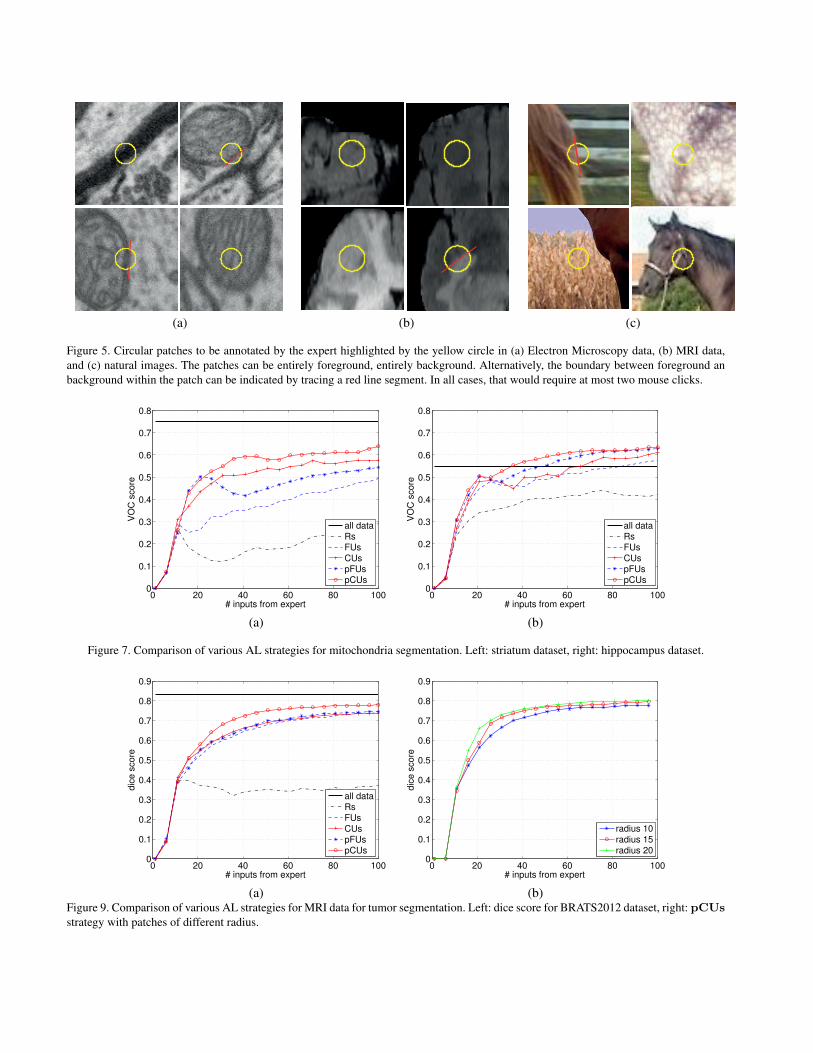
In Fig. 7, we plot the performance of all the approacheswe consider in terms of the VOC [6] score, a commonlyused measure for this kind of application, as a function ofthe annotation effort. The horizontal line at the top depictsthe VOC scores obtained by using the whole training set,which comprises 276130 and 325880 supervoxels, for thestriatum and the hippocampus respectively. FUs provides aboost over Rs, and CUs yields a larger one. In both cases, afurther improvement is obtained by introducing the batch-mode geometry query selection of pFUs and pCUs, withthe latter coming on top. Recall that these numbers are aver-ages over many runs. In Table 1, we give the correspondingvariances. Note that both using the Geometric Uncertaintyand the batch-mode tend to reduce them, thus making theprocess more predictable. Note also the 100 number we usevery much smaller than the total number of available sam-ples.

Somewhat surprisingly, in the hippocampus case, theclassifier performance given only 100 training data points ishigher that the one obtained by using all the training data.In fact, this phenomenon has been reported in the AL lit-erature [26] and suggests that a well chosen subset of dat-apoints can produce better generalisation performance thanthe complete set.

6.3. Results on MRI data

Here we consider multimodal brain tumor segmentationin MRI brain scans. Segmentation quality depends criticallyon the amount of training data and only highly-trained ex-perts can provide it. T1, T2, FLAIR, and post-GadoliniumT1 MR images are available in the BRATS dataset for eachone of 20 subjects [22]. We use standard filters such asGaussian, gradient filter, tensor, Laplacian of Gaussian andHessian with different parameters to compute the featurevectors we feed to our Boosted Trees.

(a)

(b)Figure 8. Examples of 3D datasets. a) Hippocampus volume formitochondria segmentation b) MRI data for tumor segmentation(Flair image).

In Fig. 9, we plot the performance of all the approacheswe consider in terms of the dice score [8], a commonly usedquality measure for brain tumor segmentation, as a functionof the annotation effort and in Table 1, we give the cor-responding variances. We observe the same pattern as inFig. 7, with pCUs again doing best.

The patch radius parameter r of Sec. 5 plays an impor-tant role in plane selection. To evaluate its influence, werecomputed our pCUs results 50 times using three differentvalues for r = 10, 15 and 20. The resulting plots are shownin Fig. 9. With a larger radius, the learning-rate is slightly

0 20 40 60 80 1000

0.1

0.2

0.3

0.4

0.5

0.6

0.7

0.8

# inputs from expert

f−score

all dataRsFUs

CUspFUspCUs

Figure 10. Comparison of various AL strategies for segmentationof natural images.

higher as could be expected from since more voxels are la-beled each time. However, as the patches become larger, itstops being clear that this can be done with only two mouseclicks and that is why we limited ourselves to radius sizesof 10 to 15.

6.4. Natural Images

Finally, we turn to natural 2D images and replace su-pervoxels by superpixels. In this case, the plane selectionof pFUs and pCUs reduces to simple selection of imagepatches in the image. In practice, we simply select super-pixels with their 4 neighbors. Increasing this number wouldlead to higher learning rates in the same way as increas-ing the patch radius r, but we restrics it to a small value toensure labelling can be done with 2 mouse clicks on aver-age. To compute image features, we use Gaussian, Lapla-cian, Laplacian of Gaussian, Prewitt, Sobel filters to filterintensity and color values, gather first-order statistics suchas local standard deviation, local range, gradient magnitudeand direction histograms, as well as SIFT features.

We plot our results on the Weizmann horse database inFig. 10 and give the corresponding variances in Table 1.The pattern is again similar to the one observed in Figs. 7and 9, with the difference between CUs and pCUs beingsmaller due to the fact that 2D batch-mode approach ismuch less sophisticated than the 3D one. Note, however,that the first few iterations are disastrous for all methods,however, plane-based methods are able to recover from itquite fast.

7. ConclusionIn this paper we introduced an approach to exploiting the

geometric priors inherent to images to increase the effec-tiveness of Active Learning for segmentation purposes. For2D images, it relies on an approach to Uncertainty Samplingthat accounts not only for the uncertainty of the predictionat a specific location but also in its neighborhood. For 3Dimage stacks, it adds to this the ability to automatically se-lect a planar patch in which manual annotation is easy todo.

We have formulated our algorithms in terms of back-ground/foreground segmentation but the entropy functionsthat we use to express our uncertainties can handle multipleclasses with little change to the overall approach. In futurework, we will therefore extend our approach to more gen-eral segmentation problems.

AcknowledgementsWe would like to thank Carlos Becker and Lucas

Maystre for useful and inspiring discussions, Agata Mosin-ska and Roger Bermudez-Chacon for their proofreading andcomments on the text.

(a) (b) (c)

Figure 5. Circular patches to be annotated by the expert highlighted by the yellow circle in (a) Electron Microscopy data, (b) MRI data,and (c) natural images. The patches can be entirely foreground, entirely background. Alternatively, the boundary between foreground anbackground within the patch can be indicated by tracing a red line segment. In all cases, that would require at most two mouse clicks.

0 20 40 60 80 1000

0.1

0.2

0.3

0.4

0.5

0.6

0.7

0.8

# inputs from expert

VO

C s

co

re

all dataRsFUs

CUspFUspCUs

0 20 40 60 80 1000

0.1

0.2

0.3

0.4

0.5

0.6

0.7

0.8

# inputs from expert

VO

C s

co

re

all dataRsFUs

CUspFUspCUs

(a) (b)

Figure 7. Comparison of various AL strategies for mitochondria segmentation. Left: striatum dataset, right: hippocampus dataset.

0 20 40 60 80 1000

0.1

0.2

0.3

0.4

0.5

0.6

0.7

0.8

0.9

# inputs from expert

dic

e s

co

re

all dataRsFUs

CUspFUspCUs

0 20 40 60 80 1000

0.1

0.2

0.3

0.4

0.5

0.6

0.7

0.8

0.9

# inputs from expert

dic

e s

co

re

radius 10

radius 15

radius 20

(a) (b)Figure 9. Comparison of various AL strategies for MRI data for tumor segmentation. Left: dice score for BRATS2012 dataset, right: pCUsstrategy with patches of different radius.

References[1] R. Achanta, A. Shaji, K. Smith, A. Lucchi, P. Fua, and

S. Suesstrunk. SLIC Superpixels Compared to State-Of-The-Art Superpixel Methods. IEEE Transactions on Pat-tern Analysis and Machine Intelligence, 34(11):2274–2282,November 2012.

[2] A. Al-Taie, H. H. K., and L. Linsen. Uncertainty Estimationand Visualization in Probabilistic Segmentation. 2014.

[3] B. Andres, U. Koethe, M. Helmstaedter, W. Denk, andF. Hamprecht. Segmentation of SBFSEM Volume Data ofNeural Tissue by Hierarchical Classification. In DAGM Sym-posium on Pattern Recognition, pages 142–152, 2008.

[4] C. Becker, R. Rigamonti, V. Lepetit, and P. Fua. SupervisedFeature Learning for Curvilinear Structure Segmentation. InConference on Medical Image Computing and Computer As-sisted Intervention, September 2013.

[5] E. Elhamifar, G. Sapiro, A. Yang, and S. S. Sasrty. A Con-vex Optimization Framework for Active Learning. In Inter-national Conference on Computer Vision, 2013.

[6] M. Everingham, C. W. L. Van Gool and, J. Winn, andA. Zisserman. The Pascal Visual Object Classes Chal-lenge (VOC2010) Results, 2010.

[7] R. Gilad-Bachrach, A. Navot, and N. Tishby. Query ByCommittee Made Real. In Advances in Neural InformationProcessing Systems, 2005.

[8] N. Gordillo, E. Montseny, and P. Sobrevilla. State of theArt Survey on MRI Brain Tumor Segmentation. MagneticResonance in Medicine, 2013.

[9] L. Grady. Random Walks for Image Segmentation. IEEETransactions on Pattern Analysis and Machine Intelligence,28(11):1768–1783, 2006.

[10] T. Hastie, R. Tibshirani, and J. Friedman. The Elements ofStatistical Learning. Springer, 2001.

[11] S. C. H. Hoi, R. Jin, J. Zhu, and M. R. Lyu. Batch Mode Ac-tive Learning and its Application to Medical Image Classi-fication. In International Conference on Machine Learning,2006.

[12] J. Iglesias, E. Konukoglu, A. Montillo, Z. Tu, and A. Crim-inisi. Combining Generative and Discriminative Models forSemantic Segmentation. In Information Processing in Med-ical Imaging, 2011.

[13] A. Joshi, F. Porikli, and N. Papanikolopoulos. Multi-ClassActive Learning for Image Classification. In Conference onComputer Vision and Pattern Recognition, 2009.

[14] A. Kapoor, K. Grauman, R. Urtasun, and T. Darrell. ActiveLearning with Gaussian Processes for Object Categorization.In International Conference on Computer Vision, 2007.

[15] D. Lewis and W. Gale. A Sequential Algorithm for TrainingText Classifiers. 1994.

[16] Q. Li, Z. Deng, Y. Zhang, X. Zhou, U. V. Nagerl, and S. T. C.Wong. A Global Spatial Similarity Optimization Schemeto Track Large Numbers of Dendritic Spines in Time-LapseConfocal Microscopy. IEEE Transactions on Medical Imag-ing, 30(3):632–641, 2011.

[17] T.-Y. Lin, M. Maire, S. Belongie, J. Hays, P. Perona, D. Ra-manan, P. Dollar, and C. Zitnick. Microsoft COCO: Com-

mon objects in context. In European Conference on Com-puter Vision, pages 740–755, 2014.

[18] C. Long, G. Hua, and A. Kapoor. Active Visual Recogni-tion with Expertise Estimation in Crowdsourcing. In Inter-national Conference on Computer Vision, 2013.

[19] L. Lovasz. Random Walks on Graphs: A Survey. Combina-torics, Paul Erdos is Eighty, 1993.

[20] A. Lucchi, K. Smith, R. Achanta, G. Knott, and P. Fua.Supervoxel-Based Segmentation of Mitochondria in EM Im-age Stacks with Learned Shape Features. IEEE Transactionson Medical Imaging, 31(2):474–486, February 2012.

[21] J. Maiora and M. G. na. Abdominal CTA Image Analy-sis through Active Learning and Decision Random Forests:Aplication to AAA Segmentation. In IJCNN, 2012.

[22] B. Menza, A. Jacas, et al. The Multimodal Brain Tumor Im-age Segmentation Benchmark (BRATS). IEEE Transactionson Medical Imaging, 2014.

[23] S. D. Olabarriaga and A. W. M. Smeulders. Interaction in theSegmentation of Medical Images : A Survey. Medical ImageAnalysis, 2001.

[24] F. Olsson. A Literature Survey of Active Machine Learn-ing in the Context of Natural Language Processing. SwedishInstitute of Computer Science, 2009.

[25] B. Schmid, J. Schindelin, A. Cardona, M. Longair, andM. Heisenberg. A High-Level 3D Visualization API for Javaand ImageJ. BMC Bioinformatics, 11:274, 2010.

[26] G. Schohn and D. Cohn. Less is more: Active learning withsupport vector machines. In ICML, 2000.

[27] B. Settles. Active Learning Literature Survey. ComputerSciences Technical Report 1648, University of Wisconsin–Madison, 2010.

[28] B. Settles. From Theories to Queries : Active Learning inPractice. Active Learning and Experimental Design, 2011.

[29] B. Settles, M. Craven, and S. Ray. Multiple-Instance Ac-tive Learning. In Advances in Neural Information ProcessingSystems, 2008.

[30] R. Sznitman, C. Becker, F. Fleuret, and P. Fua. Fast ObjectDetection with Entropy-Driven Evaluation. In Conferenceon Computer Vision and Pattern Recognition, pages 3270–3277, 2013.

[31] R. Sznitman and B. Jedynak. Active Testing for Face Detec-tion and Localization. IEEE Transactions on Pattern Analy-sis and Machine Intelligence, 32(10):1914–1920, June 2010.

[32] S. Tong and D. Koller. Support Vector Machine ActiveLearning with Applications to Text Classification. MachineLearning, 2002.

[33] A. Top, G. Hamarneh, and R. Abugharbieh. Active learningfor interactive 3D image segmentation. Conference on Med-ical Image Computing and Computer Assisted Intervention,2011.

[34] A. Vezhnevets, J. Buhmann, and V. Ferrari. Active Learningfor Semantic Segmentation with Expected Change. In Con-ference on Computer Vision and Pattern Recognition, 2012.