Introducing the Morningstar Solvency Score,

A Bankruptcy Prediction Metric

Warren Miller

Morningstar, Inc.

December 2009

1

Abstract This paper examines the performance of the Morningstar Solvency Score, Morningstar’s new accounting-ratio based metric for predicting bankruptcy, in comparison to the Altman Z-Score and Distance to Default models. Specifically we tested the following:

1. The ordinal ability of each model to distinguish companies most likely to file for bankruptcy from those least likely to file for bankruptcy as measured by the Accuracy Ratio

2. The cardinal ability of each model to predict bankruptcy as measured by the bankruptcy rate of healthy-scored companies and the average rating before bankruptcy

3. The decay of the ordinal performance of each model over time as measured by the cumulative percentage change in Ordinal Score

4. The stability of the ratings of each model as measured by the Weighted Average Drift Distance

We found that the Morningstar Solvency Score has superior ordinal and cardinal bankruptcy prediction power than our comparison models within a one year time horizon. It also exhibited a lower drift rate than Distance to Default, although it had less signal durability. The Solvency Score also exhibits low correlation to the Distance to Default and TLTA models, suggesting that it incorporates enough unique information to be useful in combination with the other models. Our testing universe consisted of both manufacturing and non-manufacturing companies, although we did exclude financial firms. We are cognizant that the Z-Score was never intended to gauge the financial health of non-manufacturing companies. However, it is often used to gauge the health of non-manufacturing companies in practice. Therefore we found it more relevant to test all of our models against a universe inclusive of non-manufacturing companies.

Introduction Forecasting a debtor’s ability to repay its financial obligations is a crucial endeavor for lenders and investors. Answering the question, "How likely is it that my loan will be repaid on time," is central to the valuation and asset allocation of debt portfolios. Particularly in light of recent turmoil in the credit markets, it is important that investors have the most powerful tools available for evaluating creditworthiness. Consequently, we have developed the Morningstar Solvency Score (MSS) which has demonstrated superior ordinal and cardinal predictive ability compared to the Altman Z-Score or Distance to Default. We created the Morningstar Solvency Score using stepwise logistic regression analysis. This process allowed us to test many potentially credit-relevant explanatory variables and discard those that do not improve the predictive ability of the model. The analysis yielded an intuitively appealing solution by choosing four credit-relevant explanatory variables,each of which describes a different facet of a company’s ability to meet its financial obligations (capital structure, interest coverage, profitability, and liquidity). All of our tests were performed on a testing set exclusive of the data set used to fit the model (i.e. all results displayed in this paper are out-of-sample).

2

The Z-Score, developed by Professor Edward Altman et al, is perhaps the most widely known and used model for predicting financial distress (Calandro 2007). Professor Altman developed this intuitively appealing scoring method at a time when traditional ratio analysis was losing favor with academics (Altman 2002). Using multiple discriminant analysis, Altman narrowed a list of 22 potentially significant ratios to five that, as a set, proved significant in predicting bankruptcy in his sample of 66 corporations (33 bankruptcies and 33 non-bankruptcies). Subsequent literature has criticized the Z-Score as a poorly fit model. Specifically, although each individual ratio used as predictors in the Z-Score is believed to have some bankruptcy prediction ability, the coefficients in the Z-Score calculation weaken its predictive ability to the point where it performs no better than its most predictive predictor variable (Shumway 1999). Since the development of the Z-Score, financial innovation has paved the way for further development of corporate bankruptcy prediction models. The option pricing model developed by Black and Scholes in 1973 and Merton in 1974 provided the foundation upon which structural credit models were built. KMV, now Moody’s KMV, was the first to commercialize the structural bankruptcy prediction model in the late 1980s. The Distance to Default is not an empirically created model, but rather a mathematical conclusion based on the assumption that a company will default on its financial obligations when its assets are worth less than its liabilities. It is also based on all of the assumptions of the Black-Scholes option pricing model, including for example, that asset returns are log-normally distributed. There are many dimensions upon which to measure the performance of a credit scoring system, but the most relevant way to compare models with different sample sets is by measuring the models’ ordinal ability to differentiate between companies that are most likely to go bankrupt from those that are least likely to go bankrupt (Bemmann 2005). For this reason, our primary performance indicator is the Accuracy Ratio. The Accuracy Ratio, as defined in Appendix A, is the ratio of the area between the non-predictive (random 45 degree) line and the scoring system’s curve, and the non-predictive line and the ideal scoring system’s curve in a cumulative accuracy profile. A cumulative accuracy profile plots the cumulative percentage of the bankruptcy sample that had less than or equal to a given rating prior to bankruptcy. A perfect scoring system will have an Accuracy Ratio of one. Our secondary performance test gauges each model’s cardinal ability to predict bankruptcy by comparing the average score prior to bankruptcy and the bankruptcy rate of healthy-rated companies for each model. Ideally, a credit rating model would have a very "dangerous" average rating on companies that go bankrupt and have a bankruptcy rate of zero for "safe" rated companies. In addition, we look graphically at the type I and type II errors that occur in each model. It is also important to know how quickly the predictive power of each model’s rating decays. To test this, we have created the Ordinal Score, defined in Appendix A, which measures a company’s ordinal predictive ability over time. The slower the decay of a model’s Ordinal Score, the earlier the model will warn of potential financial distress, and the more useful it can be to potential investors. Finally, rating stability is key to several of the possible applications of a credit scoring system. Because large corporate debt investors are often required to meet regulatory standards dictating the

3

credit-quality asset allocation of their portfolios, volatile ratings would increase the transaction and portfolio monitoring costs for such investors. In most models, ordinal and cardinal accuracy are at odds with rating stability, i.e. accuracy must be sacrificed for stability and vice versa (Cantor Mann 2006). To test rating stability we created drift tables, as defined in Appendix A, from which we could calculate a weighted average drift over several time periods. The lower the weighted average drift, the more stable the model’s ratings are.

Model Descriptions

Morningstar Solvency Score The Morningstar Solvency Score is an accounting-ratio based metric. Four ratios comprise the score, each of which describes a different credit-relevant characteristic of a company. These four characteristics are capital structure leverage, interest coverage, short term liquidity, and profitability. However, rather than use raw ratios which can be problematic when developing an equation via regression analysis, we transformed the ratios into percentiles based on breakpoints that uniformly distributed our entire multi-year dataset. The MSS is constructed as shown in Equation 1, and all accounting values used are those most recently available in public financial statements.

( ) ( ) ( )PPPP ROICQREBIETLTAMSS ×+×+××= 5.145 (1)

Where:

AssetsTotal

sLiabilitieTotalofScorePercentileTLTAP =

ExpenseInterest

EBITDAofScorePercentileEBIEP −= 101

RatioQuickScoreofPercentileQRP −= 101

CapitalInvestedonturnofScorePercentileROICP Re101−=

Distance to Default Morningstar’s Distance to Default score is a slightly modified structural model similar to those created by Black, Scholes and Merton and commercialized by KMV (now Moody’s KMV). Underlying the structural model is the assumption that a company’s equity can be considered an option with a strike price equal to the book value of its liabilities and a market price equal to the market value of its assets. This implies that a company is worth nothing, i.e. it has defaulted, when the market value of the assets drops below the book value of the liabilities. Based on the current market value of a company’s assets, the historical volatility of those assets, and the current book value of a company’s liabilities, one can calculate the Distance to Default using the slightly modified Morningstar methodology described in Appendix B. Unlike the Z-Score or MSS, this model does not specifically address the cash accounting values that are typically examined in a default or

4

bankruptcy scenario. In addition, the Distance to Default model does not examine the financial covenants that would be the true determinants of whether or not a distressed company defaults on its obligations.

Z-Score

The Z-Score model, commonly referred to as the Altman Z-Score, was developed by Professor Edward I. Altman in 1968 (Altman 2006). Although Altman et al have subsequently modified the original Z-Score model to create the Z’-Score Model, the Z"-Score Model, and the Zeta Model, the Z-Score model is still a common component of many credit rating systems, and is relevant as a benchmark for the Distance to Default model because of the wealth of research that has been performed on the Z-Score as well as the general academic and practical familiarity with the Z-Score. The Z-Score is constructed from six basic accounting values and one market based value. These seven values are combined into five ratios which are the pillars that comprise the Z-Score. The five pillars are combined using Equation 2 to result in a company’s Z-Score (Altman 2006).

54321 0.16.03.34.12.1 XXXXXZ ++++= (2)

Where:

AssetsTotal

CapitalWorkingX =1

AssetsTotal

EarningstainedX

Re2 =

AssetsTotal

EBITTaxesandInterestBeforeEarningsX

)(3 =

sLiabilitieTotalofValueBook

EquityofValueMarketX =4

AssetsTotal

SalesX =5

ScoreorIndexOverallZ =

This formula appeals to the practitioner’s intuition because each pillar describes a different credit-relevant aspect of a company’s operations. Liquidity, cumulative profitability, asset productivity, market based financial leverage, and capital turnover are addressed by the five ratios respectively. The Z-Score presumes that each ratio is linearly related to a company’s probability of bankruptcy.

Data Collection and Refinement The first and most important endeavor in our data collection process was to construct the largest possible list of date-company pairings for corporate bankruptcy filings. Specifically, we define the bankruptcy date as the date that the company filed for either Chapter 7 or Chapter 11 bankruptcy protection. We sourced such corporate bankruptcy data from Bloomberg’s corporate action

5

database to arrive at a list of 502 date-company pairings corresponding to bankruptcies filed between March 1998 and June 2009. This served as our "Master Bankruptcy List." Morningstar Solvency Score

The Morningstar Solvency score is comprised of the four accounting ratios described in Equation 1. These four ratios are comprised of six individual data points. Using Morningstar’s proprietary Equity XML Output Interface (Equity XOI) database as our data source, we pulled all available fiscal-year-end ratios dating back to 1998 for the 23,069 companies listed in our database. Each company-date pairing that did not include all six relevant data points was expunged from the data set. From the remaining data, the relevant ratios were constructed and used to calculate a Morningstar Solvency Score for each company-date according to Equation 1. Forty-two bankruptcies from the Master Bankruptcy List were within one year of a company-date-Z-Score record. Distance to Default

The Center for Research in Security Prices (CRSP) at the University Of Chicago Booth School Of Business provided us with a set of company-date-Distance to Default records at an annual frequency dating back to 1965. The Distance to Default was calculated in accordance with Morningstar’s published methodology paper (Morningstar 2008) included in Appendix B. CRSP’s exact methodology can be viewed in Appendix C. 56 bankruptcies from the Master Bankruptcy List were within one year of a company-date-Z-Score record. Z-Score

The Z-Score involves five ratios derived from a total of seven raw data points. These ratios are shown in Equation 2. Using Morningstar’s proprietary Equity XML Output Interface (Equity XOI) database as our data source, we pulled all available fiscal-year-end ratios dating back to 1998 for the 23,069 companies listed in our database. Each company-date pairing that did not include all seven relevant data points was expunged from the data set. From the remaining data, the relevant ratios were constructed and used to calculate a Z-Score for each company-date according to Equation 2. A total of 165 bankruptcies from the Master Bankruptcy List were within one year of a company-date-Z-Score record. Percentile Transformation

For all of our analyses, we transformed each rating system into a set of percentiles. The percentile breakpoints for each model were calculated using all available data points spanning all available time periods. As a result, the percentile ratings in any particular year are not necessarily uniformly distributed. However, this allows direct comparison of the performance of a company in the nth decile in one year with a company in the 10th decile of another year. Across all data sets, the higher the percentile (or decile or quintile as the results dictate), the more dangerous and less safe the company is rated (i.e. it is rated as having a higher probability of bankruptcy). Caveats

Because the available data for our Altman model, Distance to Default model, and TLTA model did not all include completely identical company-date pairings, each data set is unique, despite the fact that they are derived from the same set of bankruptcy data. As a result, the exposure to different risk factors, such as company size, company age, industry, etc. may differ from sample to sample.

6

Consequently, this may have a destabilizing impact on the results of our models by reducing the comparability of the results. Our use of ordinal performance as our primary comparison tool should mitigate the differences in bankruptcy rates between the samples. In addition, our Master Bankruptcy List was not comprehensive. The bankruptcies that did occur but were missing from our data set could have had a material impact on our results had they been included. Finally, our testing universe consisted of both manufacturing and non-manufacturing companies, excluding financial firms. We are cognizant that the Z-Score was never intended to gauge the financial health of non-manufacturing companies. However we find that it is often used to gauge the health of non-manufacturing companies in practice. Therefore we found it more relevant to test all of our models against a universe inclusive of non-manufacturing companies.

Model Performance

Ordinal Results

0%

10%

20%

30%

40%

50%

60%

70%

80%

90%

100%

1 6 11 16 21 26 31 36 41 46 51 56 61 66 71 76 81 86 91 96

Rating Percentile

Cum

ulative Defau

lt Perce

ntag

e

Ideal

MSS

DistanceToDefault

Z-Score

TLTA

No Predictive Ability

Figure 1: Cumulative Accuracy Profile The cumulative accuracy profile shown in Figure 1 provides more detail than the Accuracy Ratio alone. Specifically, we know from looking at the cumulative accuracy profile that the Morningstar Solvency Score is the best ordinal predictor of bankruptcy at the more dangerous end of the ratings scale, and that the Z-Score holds its own against the Distance to Default and is superior to our

7

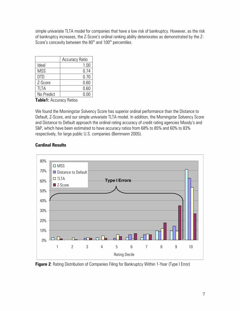
simple univariate TLTA model for companies that have a low risk of bankruptcy. However, as the risk of bankruptcy increases, the Z-Score’s ordinal ranking ability deteriorates as demonstrated by the Z-Score’s concavity between the 80th and 100th percentiles.

Accuracy Ratio

Ideal 1.00

MSS 0.74

DTD 0.70

Z-Score 0.60

TLTA 0.60

No Predict 0.00

Table1: Accuracy Ratios We found the Morningstar Solvency Score has superior ordinal performance than the Distance to Default, Z-Score, and our simple univariate TLTA model. In addition, the Morningstar Solvency Score and Distance to Default approach the ordinal rating accuracy of credit rating agencies Moody’s and S&P, which have been estimated to have accuracy ratios from 68% to 85% and 60% to 83% respectively, for large public U.S. companies (Bemmann 2005). Cardinal Results

0%

10%

20%

30%

40%

50%

60%

70%

80%

1 2 3 4 5 6 7 8 9 10

Rating Decile

MSS

Distance to Default

TLTA

Z-ScoreType I Errors

Figure 2: Rating Distribution of Companies Filing for Bankruptcy Within 1-Year (Type I Error)

8

Ideally, companies that go bankrupt within one year should all be in the 10th decile of a rating system, with no soon-to-be bankrupt companies rated in the 9th decile or below. Figure 2 shows the occurrence of false-negatives, or how often each model says a company is safe, when in-fact it is not. Graphically, we can see that the Morningstar Solvency Score and the Distance to Default outperform TLTA, which outperforms the Z-Score.

Figure 3: Rating Distribution of Companies Not Filing for Bankruptcy Within One Year (Type II Error) Figure 3 is the inverse of Figure 2. It shows the occurrence of false-positives, which are clearly quite prevalent in all four models. Ideally the graph, which shows the rating distribution for companies that did not go bankrupt within one year, would have the largest percentage of companies rated in the 1st decile, and decrease as the decile increases. We do see this relationship slightly; however, the distribution of ratings is close to uniform as all deciles are within one percentage point of each other for all four models.

Average Rating Before Default Default Rate of Top Quintile

Solvency Score 9.2 0.0%

Distance to Default 9.1 0.5%

Z-Score 8.3 0.6%

TLTA 8.2 0.8%

Table 2: Cardinal Accuracy Measures Of the four models, the Morningstar Solvency Score proved to be most predictive of bankruptcy in absolute terms, as shown in Table 2. On average, the most recent Solvency Score decile before a bankruptcy event was 9.2. In addition, it had the lowest occurrence of bankruptcies in its best rated

10%

10%

10%

10%

10%

10%

10%

1 2 3 4 5 6 7 8 9 10

Rating Decile

MSSDistance to DefaultTLTAZ-Score

Type II

Errors

9

quintile of companies. Distance to Default placed second in both measures, followed by the Z-Score and TLTA. Durability Results

As time passes, the information contained in the inputs of any particular model becomes stale. As a result, it is reasonable to expect that the ordinal ability of any bankruptcy prediction model would decay as the allowable time horizon for bankruptcy lengthens. Figure 4 shows the ordinal score of all three models over one to ten year bankruptcy time horizons. The ordinal score is defined in Appendix A, and can take on a value from 1(least ordinal ability) to 10 (most ordinal ability).

6

6.5

7

7.5

8

8.5

9

9.5

1 2 3 4 5 6 7 8 9 10Years

Ordinal Sco

re

MSS

Distance to Default

TLTA

Z-Score

Figure 4: Ordinal Score Over All Bankruptcy Time Horizons Between 1 and 10 Years Figure 4 shows that the Solvency Score has superior ordinal ability over a one-year time horizon than the other three models. However, Distance to Default bests the Solvency Score for bankruptcy time horizons greater than one year. Both the Solvency Score and Distance to Default are superior to the TLTA and Z-Score over all time horizons. Over short (<2-year) and long (>5-year) time horizons the TLTA model is superior to the Z-Score model.

10

-25%

-20%

-15%

-10%

-5%

0%

1 2 3 4 5 6 7 8 9 10

Years

Cum

ulative % Cha

nge in Ordinal Sco

re

MSS

Distance to Default

TLTA

Z-Score

Figure 5: Ordinal Score Decay Over All Bankruptcy Time Horizons Between 1 and 10 Years The cumulative change in ordinal score in Figure 5 shows us the durability of the ordinal rating each model generates. Distance to Default generates the most durable ratings because its ordinal score decays the slowest of the three models. Initially the Solvency ScoreTM and TLTA model decay at a rapid rate, but their asymptotic slopes level off over longer time periods, allowing them to outperform the Z-Score in rating durability beyond seven years. Drift Results

Many users of credit scoring systems value rating stability. Regulatory or client requirements often require debt investors to maintain a certain portfolio allocation of "safe" credit instruments. For ratings to constantly flux from "safe" to "dangerous" would cause increasing portfolio management costs to such credit market investors through increased transactions and portfolio monitoring. We measured rating stability with our measure known as Weighted Average Drift Distance, which is defined in Appendix A. It can take on values from 0 (least drift, most stable) to 9 (most drift, least stable).

11

0.0

0.5

1.0

1.5

2.0

2.5

3.0

3.5

1 3 5

Time Frame (Years)

Weighted Average Drift Distance

TLTA

Z-Score

MSS

Distance to Default

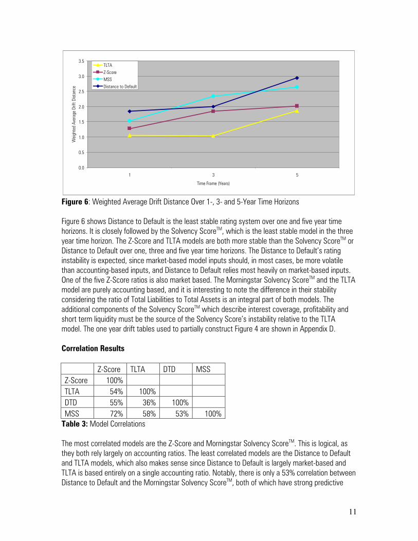
Figure 6: Weighted Average Drift Distance Over 1-, 3- and 5-Year Time Horizons

Figure 6 shows Distance to Default is the least stable rating system over one and five year time horizons. It is closely followed by the Solvency ScoreTM, which is the least stable model in the three year time horizon. The Z-Score and TLTA models are both more stable than the Solvency ScoreTM or Distance to Default over one, three and five year time horizons. The Distance to Default’s rating instability is expected, since market-based model inputs should, in most cases, be more volatile than accounting-based inputs, and Distance to Default relies most heavily on market-based inputs. One of the five Z-Score ratios is also market based. The Morningstar Solvency ScoreTM and the TLTA model are purely accounting based, and it is interesting to note the difference in their stability considering the ratio of Total Liabilities to Total Assets is an integral part of both models. The additional components of the Solvency ScoreTM which describe interest coverage, profitability and short term liquidity must be the source of the Solvency Score’s instability relative to the TLTA model. The one year drift tables used to partially construct Figure 4 are shown in Appendix D.

Correlation Results

Z-Score TLTA DTD MSS

Z-Score 100%

TLTA 54% 100%

DTD 55% 36% 100%

MSS 72% 58% 53% 100%

Table 3: Model Correlations The most correlated models are the Z-Score and Morningstar Solvency ScoreTM. This is logical, as they both rely largely on accounting ratios. The least correlated models are the Distance to Default and TLTA models, which also makes sense since Distance to Default is largely market-based and TLTA is based entirely on a single accounting ratio. Notably, there is only a 53% correlation between Distance to Default and the Morningstar Solvency ScoreTM, both of which have strong predictive

12

ability. This suggests that a combination of the two ratings could create a superior bankruptcy prediction metric than either metric by itself.

Conclusion The recent credit market turmoil has underscored the need for investors to equip themselves with the most effectual tools possible for predicting corporate bankruptcy. Accordingly, we developed the Morningstar Solvency ScoreTM to serve as an empirically derived, accounting-ratio based bankruptcy indicator. We compared the Morningstar Solvency ScoreTM to the Distance to Default, Z-Score and TLTA models for their ordinal and cardinal bankruptcy prediction abilities, rating durability over time, and rating stability. On an ordinal basis, the Solvency ScoreTM outperformed all other models when predicting bankruptcies within a one year time horizon. Distance to Default was the second best ordinal predictor, followed by the Z-Score and the TLTA ratio. Curiously, the Z-Score’s ordinal ability is nearly equal to the other two models when ranking relatively safe companies, but performs worse in situations where the probability of bankruptcy is high. All four models were found to have significant Type I errors by classifying a large number of companies that did not go bankrupt as potentially dangerous. But the Morningstar Solvency ScoreTM had superior cardinal performance as it had both a higher average rating before bankruptcy, and lower bankruptcy rate for "safe" rated companies than any one of the other three models. Rating durability is essential for a bankruptcy prediction model to generate actionable results. If the signal decays too rapidly to act upon, the model is useless in practice. We found that all four models produced actionable scores. However, Distance to Default generated more durable ratings as its ordinal score was higher over all bankruptcy time-horizons and decayed at a slower pace than either of the other two models. The Solvency ScoreTM was second-best in rating durability, outperforming the Z-Score and TLTA models. Finally, rating stability is important for creditors who must meet regulatory credit-quality requirements. The Morningstar Solvency ScoreTM and Distance to Default had more volatile ratings than both the Z-Score and the TLTA model. However, the Solvency ScoreTM had more stable ratings than Distance to Default over one and five-year time horizons. This is an intuitive result because Distance to Default relies most heavily on market-based inputs, and market-based inputs are usually more volatile than accounting-based inputs. Because nearly all situations will place greater emphasis on ordinal or cardinal accuracy before worrying about stability, we recommend the use of the Morningstar Solvency ScoreTM or Distance to Default model over the Z-Score model when trying to predict corporate bankruptcies. This of course will also depend on the availability of data for each model. In addition, the low correlation among the models, particularly the more accurate Morningstar Solvency ScoreTM and Distance to Default, suggests that using a combination of the metrics may yield a superior financial health indicator.

13

References Altman, Edward I. Corporate financial distress and bankruptcy predict and avoid bankruptcy, analyze and invest in distressed debt. Hoboken, N.J: Wiley, 2006. Print. Bemmann, Martin, Improving the Comparability of Insolvency Predictions (June 23, 2005). Dresden Economics Discussion Paper Series No. 08/2005. Available at SSRN: http://ssrn.com/abstract=731644 Calandro, Joseph , Considering the Utility of Altman's Z-Score as a Strategic Assessment and Performance Management Tool. Strategy & Leadership, Vol. 35, No. 5, pp. 37-43, 2007. Available at SSRN: http://ssrn.com/abstract=1013304 Cantor, Richard Martin and Mann, Christopher, Analyzing the Tradeoff between Ratings Accuracy and Stability. Journal of Fixed Income, September 2006. Available at SSRN: http://ssrn.com/abstract=996019 Miller, Warren, Comparing Models of Corporate Bankruptcy Prediction: Distance to Default vs. Z-Score (July 1, 2009). Available at SSRN: http://ssrn.com/abstract=1461704 Morningstar, Inc., Stock Grade Methodology for Financial Health (March 26, 2008). Morningstar Methodology Paper. Available at Morningstar: http://corporate.morningstar.com/US/asp/detail.aspx?xmlfile=276.xml Shumway, Tyler, Forecasting Bankruptcy More Accurately: A Simple Hazard Model (July 16, 1999). Available at SSRN: http://ssrn.com/abstract=171436 or doi:10.2139/ssrn.171436

14

Appendix A: Definition of Terms Cumulative Accuracy Profile (CAP): A graph of cumulative percentage of bankruptcies on the y-axis against the ordinal scoring system on the x-axis. Accuracy Ratio: The ratio of the area between the non-predictive line and the scoring system line and the area between the non-predictive line and the ideal line in a cumulative accuracy profile graph. The higher the Accuracy Score, the better the ability of the model to distinguish companies most likely to go bankrupt from those least likely to go bankrupt. Ordinal Score: The sum-product of the decile scores and the percentage of bankruptcies within x years corresponding to each decile. The higher the Ordinal Score, the better the ability of the model to distinguish companies most likely to go bankrupt from those least likely to go bankrupt.

∑ =×=

10

1 ,i xix iPBKScoreOrdinal

Where:

bankruptwentthatcompaniesofTotal

yearsxwithinbankruptwentthatidecileincompaniesofPBK xi

#

#, =

This Ordinal Score can take on continuous values from 1 (least ordinal ability) to 10 (most ordinal ability). Weighted Average Drift Distance: The sum-product of the percentage of ratings that moved from the old rating decile to a new one, and the distance of the new rating decile from the old rating decile.

( )( )∑ ∑= =

−×=

10

1

10

1

,

i j

ji ijPRCWADD

Where:

idecileinstartedthatcompaniesof

jdeciletoidecilefrommovedthatcompaniesofPRC ji

#

#, =

The Weighted Average Drift Distance can take on continuous values from 0 (no drift, maximum stability) to 10 (complete drift, no stability).

Drift Table: A table depicting the percentage of companies that started with one credit rating and ended with another for each possible starting rating. When the starting ratings are the rows of the table and the ending ratings are the columns, the rows should sum to 100%.

15

Appendix B: Morningstar’s Distance to Default Methodology Structural models take advantage of both market information and accounting financial information. For this purpose, option pricing models based on seminal works of Black and Scholes (1973) and Merton (1974) are a natural fit. The firm's equity can be viewed as a call option on the value of the firm's assets. If the value of assets is not sufficient to cover the firm's liabilities, the strike price, default is expected to occur, and the call option expires worthless, and the firm is turned over to its creditors. Asset Value = Equity Value + Liabilities (1) The underlying premise of contingent claim models is that default occurs when the value of the firm's assets falls below a certain threshold level relative to the firm's liabilities. According to Merton (1974) if the firms liabilities consist of one zero-coupon bond with notional value L, maturing in T (without any debt payment until T), and equity holders wait until T (to benefit from expected increase of the asset value), the default probability, at time T, is that the value of assets is less than the value of the liabilities. To estimate this probability, the value of the firm's liability is obtained from the firm's latest balance sheet. Lt = Ls + Ll (2) Where: Lt = Total Liability Ls = Short Term Liability Ll = Long Term Liability Next, the probability distribution of firm's assets value at time T needs to be estimated. It is assumed that the value of firm's assets follow a log-normal distribution, i.e. the logarithm of the firm's asset value is normally distributed and the expected change in log asset values is µ - δ -

σ 2 / 2. The log asset value in T year therefore follows a normal distribution with following parameters:

ln AT ≈N [ ln At + ( µ - δ - σ A2 / 2) (T - t) , σ A

2 (T – t)] (4)

Where µ is the continuously compounded expected return on assets or the asset drift and

δ is asset yield, expressed in terms of current assets value and is equal to

(TTM common + preferred dividends) / Current asset value Next, the probability that a normally distributed variable x falls below z is given by

/])[{( xEzN − σ A(x)},

Where N denotes the cumulative standard normal distribution.

16

To empirically estimate the Black-Scholes probability from equation (4), we need estimates of: At, µ

and σ A which are not directly observable. Though if they were known there would be no need for

using Black-Scholes and the probability of bankruptcy (PB) and Distance to default (DD), can be expressed (McDonald 2002) as:

PB = N{ - [[ ln At – ln Lt + ( µ - δ - σ A2 / 2) (T-t)] / [σ A )( tT − ]]}

= N{ - [[ ln (At / Lt) + ( µ - δ - σ A2 / 2) (T-t)] / [σ A )( tT − ]]} (5)

DD = [ ln At + (µ - δ - σ A2 / 2) (T – t) – ln Lt)] / σ A )( tT − (6)

=> PB = N [ -DD] (7) Equation (5) shows that probability of bankruptcy is a function of the distance between the value of firm's assets today and the book value of firm's total liabilities, (At / Lt) adjusted for the expected growth in asset value, asset drift, and asset yield, ( µ - δ - σ A

2 / 2) relative to asset volatility,σ A.

But the market value of the firm's assets is not observable and can be very different than the book value of the firm's assets. This is the At in equation (5). Furthermore, we do not know the volatility of the market value of the firm's assets, nor we can use the observed asset values (book values) as a proxy of the firm's market value of assets volatility,σ A. That's where the option pricing comes in

since it implies a relationship between the unobservable (At, σ A) and the observable variables. As long as value of the firm's assets is less than the book value of the firm's liabilities, the payoff to equity holders is zero. If the value of the firm's assets is higher than book value of the firm's liabilities, equity holders receive the residual value and their payoff increases linearly as value of the firm's assets increase over time. This can be expressed as payoff of a modified (for dividends) European call option: ET = Max (0, AT – Lt ) (8) Assuming risk-neutrality, the equity value, Et, can be estimated by a modified (for dividends) standard Black-Scholes call option formula: Et = At e

-δ T* N (d1) – Lt * e

– rT * N (d2) + ( 1 - e-δ T) At (9)

Where r is the safe rate (one year treasury yield), and N (d1) and N

(d2) are the cumulative standard normal of d1 and d2.

Dividend yield,δ , added to the standard Black-Scholes model in equation (9), which appears twice

in the right hand side of the equation. First, term At e-δ T accounts for the reduction in the value of

17

firm's assets due to dividends that are distributed at time T. Second, term ( 1 - e-δ T) At accounts

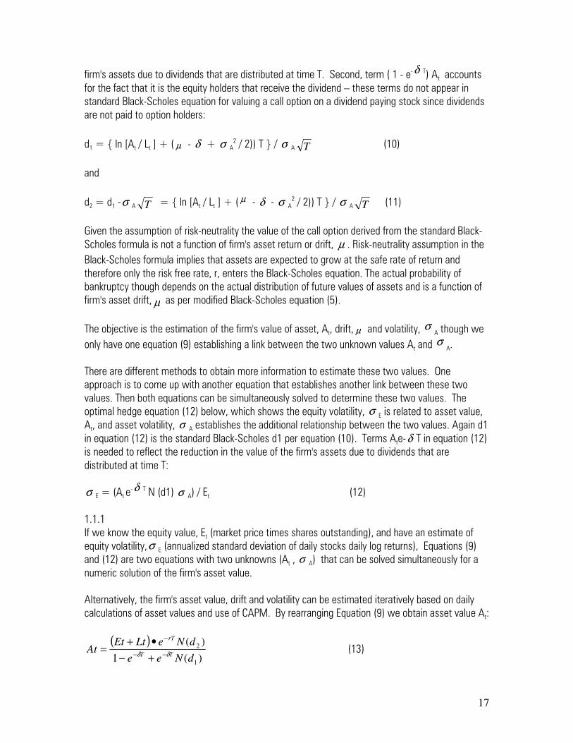
for the fact that it is the equity holders that receive the dividend – these terms do not appear in standard Black-Scholes equation for valuing a call option on a dividend paying stock since dividends are not paid to option holders:

d1 = { ln [At / Lt ] + ( µ - δ + σ A2 / 2)) T } / σ A T (10)

and

d2 = d1 -σ A T = { ln [At / Lt ] + ( µ - δ - σ A2 / 2)) T } / σ A T (11)

Given the assumption of risk-neutrality the value of the call option derived from the standard Black-Scholes formula is not a function of firm's asset return or drift, µ . Risk-neutrality assumption in the

Black-Scholes formula implies that assets are expected to grow at the safe rate of return and therefore only the risk free rate, r, enters the Black-Scholes equation. The actual probability of bankruptcy though depends on the actual distribution of future values of assets and is a function of firm's asset drift,µ as per modified Black-Scholes equation (5).

The objective is the estimation of the firm's value of asset, At, drift, µ and volatility, σ A though we

only have one equation (9) establishing a link between the two unknown values At and σ A. There are different methods to obtain more information to estimate these two values. One approach is to come up with another equation that establishes another link between these two values. Then both equations can be simultaneously solved to determine these two values. The optimal hedge equation (12) below, which shows the equity volatility, σ E is related to asset value, At, and asset volatility, σ A establishes the additional relationship between the two values. Again d1 in equation (12) is the standard Black-Scholes d1 per equation (10). Terms Ate-δ T in equation (12) is needed to reflect the reduction in the value of the firm's assets due to dividends that are distributed at time T: σ E = (At e

-δ T N (d1) σ A) / Et (12) 1.1.1 If we know the equity value, Et (market price times shares outstanding), and have an estimate of equity volatility,σ E (annualized standard deviation of daily stocks daily log returns), Equations (9) and (12) are two equations with two unknowns (At , σ A) that can be solved simultaneously for a numeric solution of the firm's asset value. Alternatively, the firm's asset value, drift and volatility can be estimated iteratively based on daily calculations of asset values and use of CAPM. By rearranging Equation (9) we obtain asset value At:

( ))(1

)(

1

2

dNee

dNeLtEtAt

TT

rT

δδ −−

−

+−

•+= (13)

18

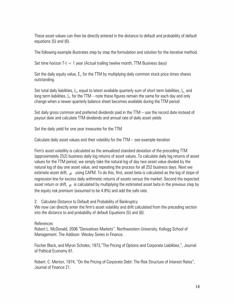
These asset values can then be directly entered in the distance to default and probability of default equations (5) and (6). The following example illustrates step by step the formulation and solution for the iterative method. Set time horizon T-t = 1 year (Actual trailing twelve month, TTM Business days) Set the daily equity value, Et, for the TTM by multiplying daily common stock price times shares outstanding. Set total daily liabilities, Lt, equal to latest available quarterly sum of short term liabilities, Ls, and long term liabilities, Ll. for the TTM – note these figures remain the same for each day and only change when a newer quarterly balance sheet becomes available during the TTM period Set daily gross common and preferred dividends paid in the TTM – use the record date instead of payout date and calculate TTM dividends and annual rate of daily asset yields Set the daily yield for one year treasuries for the TTM Calculate daily asset values and their volatility for the TTM – see example iteration Firm's asset volatility is calculated as the annualized standard deviation of the preceding TTM (approximately 252) business daily log returns of asset values. To calculate daily log returns of asset values for the TTM period, we simply take the natural log of day two asset value divided by the natural log of day one asset value, and repeating the process for all 252 business days. Next we estimate asset drift, µ using CAPM. To do this, first, asset beta is calculated as the log of slope of

regression line for excess daily arithmetic returns of assets versus the market. Second the expected asset return or drift, µ is calculated by multiplying the estimated asset beta in the previous step by

the equity risk premium (assumed to be 4.8%) and add the safe rate. 2. Calculate Distance to Default and Probability of Bankruptcy We now can directly enter the firm's asset volatility and drift calculated from the preceding section into the distance to and probability of default Equations (5) and (6).

References Robert L. McDonald, 2006 “Derivatives Markets”. Northwestern University, Kellogg School of Management. The Addison- Wesley Series in Finance. Fischer Black, and Myron Scholes, 1973,”The Pricing of Options and Corporate Liabilities,”, Journal of Political Economy 81. Robert. C. Merton, 1974, “On the Pricing of Corporate Debt: The Risk Structure of Interest Rates”, Journal of Finance 21.

19

Appendix C: CRSP’s Implementation of Morningstar’s Distance to Default Methodology

A. In case of multiple share classes, DTD is calculated for the most liquid share class as defined by the largest market cap as of the rebalancing date. Then the same DTD is assigned to other share classes of the company.

B. Distance to default (DTD) is calculated for all companies included in the size-based indices with valid daily date for at least 90 trading days. If the data for 90 trading days before the date of DTD measure calculation is not available than DTD measure is set to missing.

C. Distance to default (DTD) calculation.

Timing: quarterly rebalancing date Inputs: 252 daily values (trading days) of the following: - company market cap - company total liabilities (expressed from annual and quarterly data) - dividends - Treasury yield, annual (one-year Treasury) - market index total return (CRSP NYSE/Alternext/NASDAQ value-weighted market index) Calculation process: DTD=NormDist.Calculate(-dd); Where NormDist.Calculate(-dd); -- the probability that an observation from the standard normal distribution is less than or equal to -dd. This is the score to be used in creating distressed/non-distressed portfolios.

dd = (Log(asset/liability) + (driftRate - dividend yield - Standard Deviation^2 / 2)) / Standard Deviation Where 1. asset is the value of asset0 array as of rebalancing date. Asset0 array is initialized over 252 trading days as follows: asset0 = MarketCap + Total Liabilities (in comparable units) The final values of asset0 and asset1 arrays are generated as follows: asset1 = (MarketCap + Total Liabilities*e^(-ln(1 + riskfree rate)) * Normdist(d1 - sqrt(Standard Deviation * 252)) ) / (1+(Normdist(d1)-1)*e^(-ln(1+dividend yield))

20

Where: • d1 = (ln(asset0 / Total Liabilities) + (ln(1 + risk free rate) - ln(1 + dividend yield) + .5 * sqrt(Standard Deviation *252) ^ 2 ) * 1 year ) / (sqrt(Standard Deviation *252))* sqrt( 1 year) ) m=length(asset0) x(daily_return)i = log(asset0i+1/asset0i) i=0,...,n-1 n=m-1=length(x)

( )

1tan 0

2

−

−

=∑

=

n

xx

deviationdards

n

i

i

• dividend yield = sum (252 trading days of dividends * shares_outstanding) / value from asset0 array • Standard Deviation = 252 trading days standard deviation of asset0 array • riskfree rate = annual Treasury yield (one year Treasury) • MarketCap = price*shares_outstanding Asset1 values are stored in the asset1 array. A sum of squared errors is calculated between the asset0 array and asset1 array. If the sum of squared errors is not less than 0.01 then the values of the asset1 array are copied over the asset0 array. The process repeats until the sum of squared errors target is reached, or a maximum of 100 iterations is reached. 2. liability = TotalLiability 3. driftRate – driftRate if (expectedReturn <=0) then driftRate = riskfreeRate else driftRate = Log(1 + expectedReturn);

if (expectedReturn <=0) then driftRate = riskfreeRate else driftRate = Log(1 + expectedReturn); where expectedReturn = riskfreeRate + beta * 0.048 riskfreeRate = annual Treasury yield (one year Treasury) beta = security market beta over 252 trading day period calculated using asset0 array values, a market index, and riskfreeRate/252 i.e. CAPM regression beta from the following: (daily_asset0_return- riskfreeRate/252)=a+beta(daily_market_return- riskfreeRate/252)+e

21

driftRate is calculated as of rebalancing date after asset0 array process is completed.

D. Total Liability: The CRSP Compustat Merged Database is used to link trading securities and retrieve the company Total liability. Total liability is defined as Compustat quarterly data Item Q54 (LTQ) or Compustat annual data Item A181 if the quarterly data is not available. The best single Compustat record (excluding LS linktypes) for the company is used for Total Liabilities value. A valid Total Liability value is defined as non-missing and non-zero (negative Total Liabilities are considered valid).

Annual and Quarterly Total Liability values are used to create a single daily record with the latter taking precedence. Up to four quarters lag is used to find non-missing value to use on a given breakpoint date.

22

Appendix D: 1-Year Drift Tables

Morningstar Solvency Score

End

1-Year 1 2 3 4 5 6 7 8 9 10

1 56% 18% 10% 6% 3% 2% 2% 1% 1% 0%

2 19% 31% 19% 10% 7% 6% 4% 2% 2% 1%

3 8% 22% 22% 16% 12% 7% 4% 4% 3% 2%

4 4% 12% 18% 21% 15% 12% 8% 5% 4% 2%

Start 5 2% 6% 11% 17% 19% 15% 12% 10% 6% 3%

6 2% 3% 7% 12% 17% 18% 15% 14% 9% 5%

7 1% 2% 4% 8% 12% 17% 18% 17% 12% 9%

8 1% 2% 3% 5% 8% 13% 17% 18% 20% 13%

9 1% 1% 2% 2% 3% 8% 11% 20% 29% 24%

10 0% 1% 1% 2% 3% 4% 6% 11% 23% 48%

Distance to Default

END

1-Year 1 2 3 4 5 6 7 8 9 10

1 42% 23% 12% 9% 6% 4% 2% 2% 1% 0%

2 23% 21% 17% 13% 10% 9% 3% 3% 1% 0%

3 16% 15% 18% 15% 14% 9% 7% 3% 2% 0%

4 12% 13% 13% 15% 14% 13% 11% 7% 2% 0%

Start 5 7% 10% 12% 12% 14% 14% 13% 11% 5% 1%

6 6% 9% 10% 11% 12% 14% 15% 13% 8% 2%

7 3% 6% 7% 9% 11% 13% 14% 17% 14% 6%

8 3% 4% 6% 8% 8% 9% 13% 17% 20% 12%

9 2% 3% 6% 5% 7% 8% 10% 14% 24% 21%

10 1% 2% 2% 3% 3% 6% 6% 10% 17% 51%

Z-Score

End

1 2 3 4 5 6 7 8 9 10

1 28% 22% 13% 9% 6% 4% 4% 4% 4% 7%

2 17% 23% 17% 13% 9% 7% 4% 4% 3% 4%

3 9% 15% 19% 18% 13% 8% 5% 4% 4% 4%

4 5% 12% 17% 18% 17% 10% 8% 6% 4% 4%

Start 5 3% 7% 13% 17% 17% 15% 11% 8% 5% 4%

6 2% 4% 7% 13% 17% 19% 16% 11% 6% 5%

7 2% 2% 4% 7% 10% 18% 24% 16% 10% 6%

8 1% 2% 3% 4% 7% 14% 19% 25% 17% 7%

9 1% 2% 2% 4% 5% 6% 12% 20% 31% 17%

10 3% 2% 3% 5% 4% 6% 7% 12% 23% 33%

23

TLTA

End

1 2 3 4 5 6 7 8 9 10

1 60% 20% 6% 3% 3% 1% 1% 1% 1% 3%

2 17% 43% 19% 8% 4% 2% 1% 1% 1% 2%

3 5% 18% 37% 20% 8% 4% 2% 1% 1% 2%

4 2% 6% 19% 36% 18% 8% 4% 2% 2% 3%

Start 5 1% 3% 6% 20% 35% 18% 8% 4% 3% 3%

6 1% 2% 3% 6% 19% 37% 18% 7% 4% 3%

7 1% 1% 2% 3% 6% 19% 39% 19% 6% 5%

8 1% 1% 1% 2% 2% 5% 20% 43% 18% 7%

9 1% 1% 1% 1% 1% 3% 5% 18% 50% 20%

10 1% 1% 2% 2% 2% 2% 3% 5% 19% 63%