introduction and perspective - deohs home
TRANSCRIPT

Opportunities for Bringing Rapidly Emerging
Technologies to Revolutionize Modeling of
Chemical Contaminants of Coastal Waters
Dr. Joel Baker
Director, UW Puget Sound Institute
University of Washington Tacoma
3
Introduction and Perspective
May, 1982: Duluth, Minnesota
4
Introduction and Perspective
October, 2012: Tacoma, WA
5
The Information Technology Revolution
NJTechReviews6
The Information Technology Revolution
2010 Map of the Global Internet by Cisco Systems
7
Map data © 2012 Googl e -
To see all the details that are visible on the
screen, use the "Print" link next to the map.
seattle traffic report - Google Maps http://maps.google.com/maps?oe=utf-8&rls=org.mozilla:en-US:...The Information Technology Revolution
8

Modeling Chemical Contaminants in
Aquatic Ecosystems:
Seminal Papers in PCB Modeling
9
Modeling Chemical Contaminants in
Aquatic Ecosystems: Karickhoff et al. 1979
10
Modeling Chemical Contaminants in
Aquatic Ecosystems: Karickhoff et al. 1979
11
Modeling Chemical Contaminants in Aquatic
Ecosystems: Thomann and DiToro, 1983
12
Modeling Chemical Contaminants in Aquatic
Ecosystems: Mackay, 1989
13
Modeling Chemical Contaminants in Aquatic
Ecosystems: Mackay, 1989
14

Modeling Chemical Contaminants in Aquatic
Ecosystems: Gobas and Mackay, 1988
15
Modeling Chemical Contaminants in Aquatic
Ecosystems: Gobas and Mackay, 1988
16
Modeling Chemical Contaminants in Aquatic
Ecosystems: Current Models
R.A. Park et al., 201017
Modeling Chemical Contaminants in Aquatic
Ecosystems: NY/NJ Harbor CARP Model
Management Question
�Which sources of contaminants need to be reduced or
eliminated to render future dredged material clean?
Management Question
�Which sources of contaminants need to be reduced or
eliminated to render future dredged material clean?
18
Modeling Chemical Contaminants in Aquatic
Ecosystems: NY/NJ Harbor CARP Model
19 20

21
Summary of 2,3,7,8-TCDD
interim ““““clean bed”””” analysis
22
The Information Technology Revolution
NJTechReviews
?
CARP
23
Premise of Today’s Talk
Tools to model contaminant behavior and effects in
aquatic ecosystems have not kept up with the
information technology revolution
24
Corollaries
1. We assume that technology is frozen in time
to what tools we had available in grad school
(computers, IT, and analytical chemistry)
2. Innovation and experimentation may be seen
at odds with stability and confidence
25
Wait!
Is this really a problem?
What are we missing with current models?
26

27
Non-Spherical Cows
1. Phase partitioning in the water column
28
• Use PCB and PAH distribution coefficients
measured in the Chesapeake Bay to explore the
mechanism driving observed variability
– three-phase partitioning?
– slow sorption kinetics?
– highly sorbent particles?
29
Log KOW
3 4 5 6 7 8 9
Lo
g K
d
1
2
3
4
5
6
7
8
9
PAHsPCBs
[Mass on Filter/Volume Filtered]
Kd= -----------------------------------------------
[Mass on XAD/Volume Processed][TSS]
Log
Kd
30
Log Kd
3.84 3.97 4.11 4.24 4.37 4.50 4.64 4.77 4.90 5.03 5.17 5.30
Fre
quency
0
5
10
15
20 Pyrene
N = 119
Baltimore Harbor
Surface Waters
31
Percent Dissolved
1 6 11 16 21 26 31 36 41 46 51 56 61 66 71 76 81 86 91 96
Fre
quency
0
2
4
6
8
10
12
14
16Pyrene Fraction DissolvedN = 119Baltimore Harbor Surface Waters
32
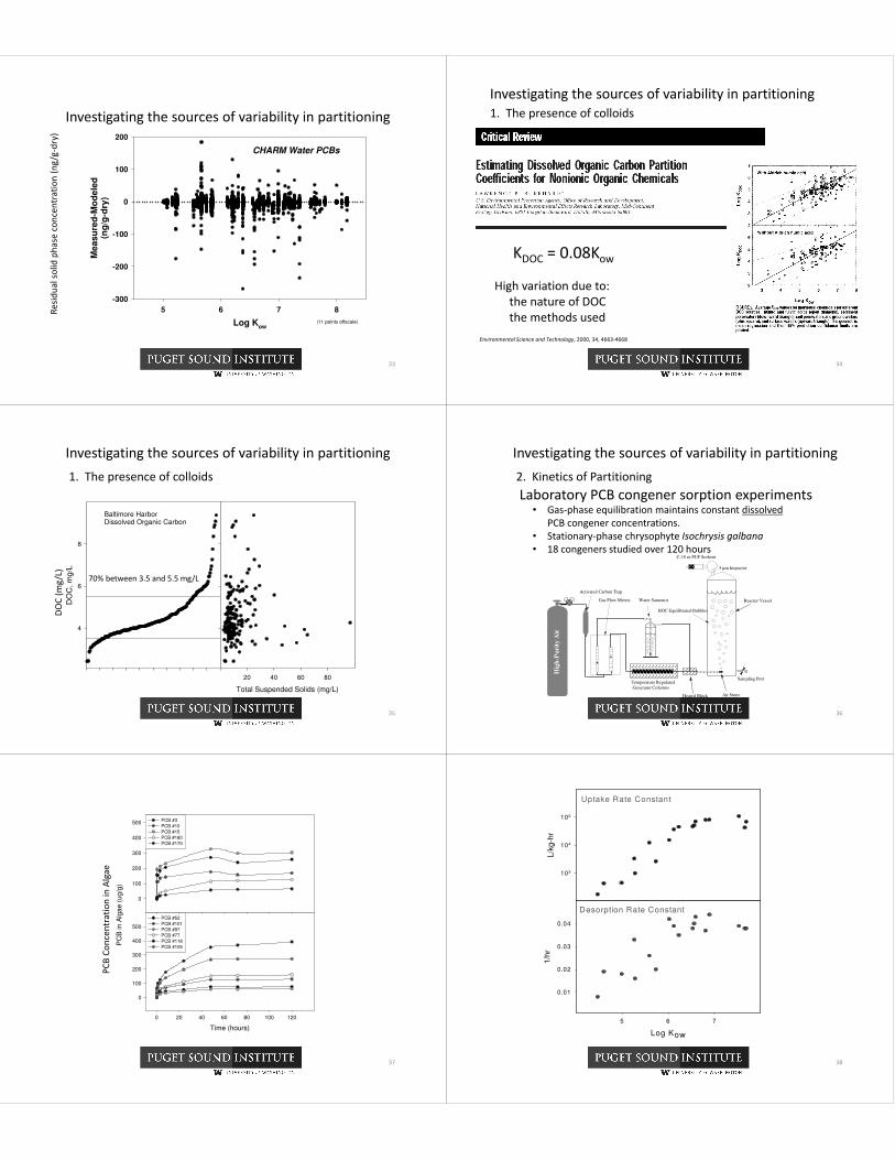
CHARM Water PCBs
Log Kow
5 6 7 8
Measu
red
-Mo
dele
d(n
g/g
-dry
)
-300
-200
-100
0
100
200
(11 points offscale)
Investigating the sources of variability in partitioning
Re
sid
ua
l so
lid
ph
ase
co
nce
ntr
ati
on
(n
g/g
-dry
)
33
KDOC = 0.08Kow
High variation due to:
the nature of DOC
the methods used
Environmental Science and Technology, 2000, 34, 4663-4668
1. The presence of colloids
Investigating the sources of variability in partitioning
34
Baltimore HarborDissolved Organic Carbon
DO
C, m
g/L
4
6
8
Total Suspended Solids (mg/L)
20 40 60 80
Investigating the sources of variability in partitioning
1. The presence of colloids
70% between 3.5 and 5.5 mg/L
DO
C (
mg
/L)
35
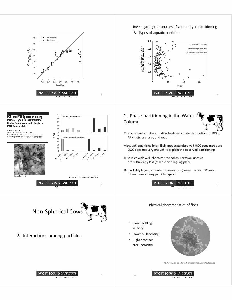
Investigating the sources of variability in partitioning
2. Kinetics of Partitioning
C-18 or PUF Sorbent
Water Saturator
5 µm Impactor
Gas Flow Meters
HOC Equilibrated Bubbles
Reactor Vessel
Temperature Regulated
Generator Columns
Heated Block
Sampling Port
Air Stone
Hig
h-P
uri
ty A
ir
Activated Carbon Trap
Laboratory PCB congener sorption experiments• Gas-phase equilibration maintains constant dissolved
PCB congener concentrations.
• Stationary-phase chrysophyte Isochrysis galbana
• 18 congeners studied over 120 hours
36
Time (hours)
0 20 40 60 80 100 120
PC
B in A
lgae (
ug/g
)
0
100
200
300
400
500
PCB #52
PCB #101
PCB #97
PCB #77
PCB #118
PCB #105
0
100
200
300
400
500 PCB #3
PCB #10
PCB #15
PCB #180
PCB #170
PC
B C
on
cen
tra
tio
n i
n A
lga
e
37
Uptake Rate Constant
L/k
g-h
r
103
104
105
Desorption Rate Constant
Log Kow
5 6 7
1/h
r
0.01
0.02
0.03
0.04
38
Log Kow
4.5 5.0 5.5 6.0 6.5 7.0 7.5
Lo
g K
oc
4.5
5.0
5.5
6.0
6.5
7.0
7.5 15 minutes
72 hours
Ob
serv
ed
Lo
g K
OC
39
Investigating the sources of variability in partitioning
3. Types of aquatic particles
TSP
0 20 40 60
Fra
cti
on
Pla
nkto
n
0.2
0.4
0.6
0.8
1.0
CHARM 01 (Fall '99)
CHARM 02 (Winter '00)
CHARM 03 (Summer '00)
Fra
ctio
n d
isso
lve
d p
yre
ne
40
41
1. Phase partitioning in the Water
Column
The observed variations in dissolved-particulate distributions of PCBs,
PAHs, etc. are large and real.
Although organic colloids likely moderate dissolved HOC concentrations,
DOC does not vary enough to explain the observed partitioning.
In studies with well-characterized solids, sorption kinetics
are sufficiently fast (at least on a log-log plot).
Remarkably large (i.e., order of magnitude) variations in HOC-solid
interactions among particle types.
42
Non-Spherical Cows
2. Interactions among particles
43
Physical characteristics of flocs
• Lower settling
velocity
• Lower bulk density
• Higher contact
area (porosity)
http://www.water-technology.net/contractor_images/cu_water/flocke.jpg
44

How are flocs formed?
Yao and O’Melia (1971)
45
Flocculation and PCB Models
• The model simulated the floc size among 2 to 1000 µm
• The multi-class flocculation model equations are based on the concept
of O’Melia (1982)
• The floc porosity and settling velocity are based on the concept of
Winterwerp (1998)
• The floc settling velocity, floc density, stickiness coefficient, and fraction
of organic carbon (fOC) are calculated simultaneously and temporally at
each class of flocculation particle
• The PCB mass transfer coefficient is varied with floc properties
46
Figure 6 c, d
Time (hour)0 10 20 30 40 50
TV
C (
m3/m
3)
0
1e-4
2e-4
3e-4
4e-4
5e-4
Predicted TVC
Measured TV
Figure 3d
PCB 52
Time (hour)
0 10 20 30 40 50
Cp
(u
g/m
3)
0
20
40
60
80
100
120
140
Model Cp
Measured Cp
Time (hour)
0 10 20 30 40 50
Cd
(u
g/m
3)
0
2
4
6
8
10
12
14
Model Cd
Measured Cd
Particulate PCB
Dissolved PCB
Total Volume Concentration
Total Suspended Solids
47
Non-Spherical Cows
3. Chemical release during resuspension
48
Desorption Rates
Engineering Performance Standards for Dredging
Volume 2: Technical Basis and Implementation of the Resuspension
Standard
• Analysis assumes first order desorption kinetics during the first day of resuspension
• Experiments show rapid (nearly instantaneous) release at onset of resuspension
Given the length of time required for PCBs to reach equilibrium for desorption, it is
unlikely that there will be large release of dissolved phase PCBs as a result of dredging
activities.
49
Objectives
• What is the initial release of PCBs from quiescent river sediment when it is resuspended (i.e. during high flow or dredging)?
• How does the frequency and duration of resuspension events affect PCB desorption?
50
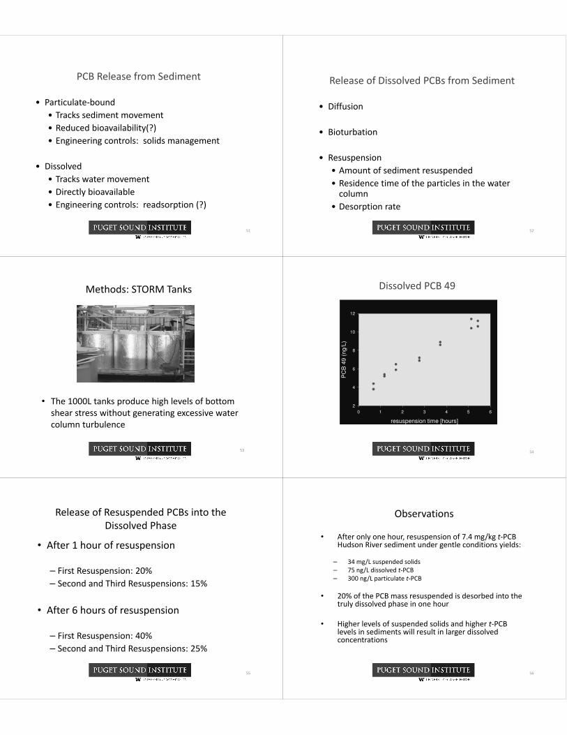
PCB Release from Sediment
• Particulate-bound
• Tracks sediment movement
• Reduced bioavailability(?)
• Engineering controls: solids management
• Dissolved
• Tracks water movement
• Directly bioavailable
• Engineering controls: readsorption (?)
51
Release of Dissolved PCBs from Sediment
• Diffusion
• Bioturbation
• Resuspension
• Amount of sediment resuspended
• Residence time of the particles in the water column
• Desorption rate
52
Methods: STORM Tanks
• The 1000L tanks produce high levels of bottom
shear stress without generating excessive water
column turbulence
53
Dissolved PCB 49
resuspension time [hours]
0 1 2 3 4 5 6
PC
B 4
9 (
ng/L
)
2
4
6
8
10
12
54
Release of Resuspended PCBs into the
Dissolved Phase
• After 1 hour of resuspension
– First Resuspension: 20%
– Second and Third Resuspensions: 15%
• After 6 hours of resuspension
– First Resuspension: 40%
– Second and Third Resuspensions: 25%
55
Observations
• After only one hour, resuspension of 7.4 mg/kg t-PCB Hudson River sediment under gentle conditions yields:
– 34 mg/L suspended solids
– 75 ng/L dissolved t-PCB
– 300 ng/L particulate t-PCB
• 20% of the PCB mass resuspended is desorbed into the truly dissolved phase in one hour
• Higher levels of suspended solids and higher t-PCB levels in sediments will result in larger dissolved concentrations
56

Observations
• A fine fraction of the sediment enriched in t-PCBs is readily resuspended and does not resettle over 12 hours. This material will likely be transported downstream.
• Both desorption kinetics and observed PCB behavior during resettling are consistent with PCB release being dominated by fine-grain particles.
57
Lessons Learned (so far…)
1.“Don’t make me come out of retirement to come back here to fix
the loadings estimates” – R. Thomann
2.“Sediment transport is a side show” – D. DiToro
Keep your eye on the ball
3.“If a simulation won’t finish overnight the model is too complex”
The modeling effort must generate something that fits on a
manager’s laptop
4.Complex systems require continual review during development
Building inspectors
58
Final Thoughts
Complex models are too expensive to develop and run too slowly to be useful
Moore’s Law and Silicon Qubits
You can’t calibrate a highly resolved model
Self-learning using real-time observations?
Sediment transport is too hard to model
In situ PSD measurements and highly resolved hydrodynamics
Nobody understand complex models
Pixar studios
59
Dr. Joel Baker
Director, UW Puget Sound Institute
University of Washington Tacoma
60
61
Links page
• Dr. Joel Baker ([email protected])
• Center for Urban Water at University of Washington Tacoma:http://www.tacoma.uw.edu/center-urban-waters
• University of Washington Superfund Research Program:http://depts.washington.edu/sfund/
• US EPA Region 10:http://www.epa.gov/aboutepa/region10.html
• National Institute of Environmental Health Institute (NIEHS)-Superfund Research Programhttp://www.niehs.nih.gov/research/supported/srp/