Cyrille Barreteau

CEA Grenoble, DSM/DRFMC/SP2M

TIGHT-BINDING METHODS

SIMPLE CONCEPTSAND

EXAMPLES

INTRODUCTION

History and vocabulary

Tight-binding : Solid State Physics point of viewMott and Jones, Slater and the pionneering works of Friedel in the60’s.

Huckel,(LCAO) : The chemists world

Semi-empirical method

1.000.000

large systemslow transferabilityno electronic structure

SIZE

transferability depends on the systemand on the parametrization‘‘reasonable size’’electronic structure

good transferability

EMPIRICAL POTENTIALS

TIGHT-BINDING (SEMI-EMPIRICAL)

AB-INITIO

small systemselectronic structure

TRANSFERABILITY

100

10.000

1000

Most tight-binding methods are parametrized. The parameters of themodel are fitted either on experimental or on ab-initio results (the mostpopular procedure nowadays).

The jungleThere is a huge number of tight-binding methods depending on :

� parametrization.

� level of approximation : orthogonal or non-orthogonal, environmentdependance..

� degree of “ab-initio”.

OVERVIEW

Electronic Structure

1) Basic principles2) Some important quantities3) A simple example : simple cubic s-band model4) Self consistent Tight-Binding5) Doing tight-binding

Total Energy1) Decomposition of the energy2) Forces3) Empirical potentials4) DFT justification

Some examples of application

BIBLIOGRAPHY

Concepts in Surface Physics (Chapter 5)M.C. Desjonquères and D. Spanjaard. Spinger Verlag

Order and Phase Stability in alloys (Chapter 6)F. Ducastelle. North Holland

Electronic Structure of MaterialsA. P. Sutton. Oxford University Press.

Electronic Structure and the Properties of Solids.W. Harrisson. Dover.

Solid State Physics : Problems and Solutions.L. Mihaly and C. Martin. Wiley-Interscience.

Tight-Binding Modelling of materials.Goringe et al. Rep. Prog. Phys. 1997.

Linear Scaling electronic structure methods.S. Goedecker. Review of Modern Physics, 1999.

BASIC PRINCIPLES

a) the basis setThe basic approximation of the tight-binding (TB) scheme is to assumethat all electronic wave function of interest can be described within aresctricted Hilbert space spanned by atomic-like orbitals.

ψ

�

r

� � ∑n �λ

cnλφλ

�

r � n

�

�

�ψ � � ∑

nλcnλ

�

nλ �

n : site index, ( n � 1 � Nat) λ : orbital index ( λ � 1 � l )

λ � s� � �1

� px � py � pz� � �

3� � �

4 : semi-conductors

� dxy � dyz � dxz � dx2 y2 � d3z2 r2� � �

5 : Transition Metals

� � �

9 : Transition Metals

Overlaps integrals

Sλ �µn �m

� � nλ

�

mµ � ��

drφλ

�

r � n

�

φµ

�

r � m

�

orthogonal tight-binding :For “convenience” it is often assumed that the TB basis is orthogonal :

Sλ �µn �m

� � nλ

�

mµ � � δnmδλµ

closure relation :

∑nλ

�

nλ � � nλ

� � Id

b) the Hamiltonian

H � T

�

Ve f f

� T

�∑n

V atn

T : kinetic energy. Ve f f : one electron potential.

� nλ

�

H

�

mµ � � � nλ

�

T

�

Vm

�

mµ � � � nλ

�

∑p

���mV at

p

�

mµ �

�

nλ � obeys the Schrodinger equation for a single atom :

Hλ �µnm

� εat �λn δmnδλ �µ

� � nλ

�

∑p

���mV at

p

�

mµ �

Three center integrals are neglected

� nλ

�

∑p

���mV at

p

�

mµ �� � nλ

�

V atn

�

mµ � � βλµnm

Intra-atomic matrix elements

Hλµnn

� εatnλδλµ

� � nλ

�

∑p

���mV at

p

�

nµ �

�

εatnλatomic level of orbital

�

nλ �

αλµn

� � nλ

�

∑p

���mV atp

�

nµ � crystal field integral �

Hλµnn

� ε0nλδλµ

Inter-atomic matrix elements :

Hλµnm

� βλµnm

�

m � n

�� n

� � m

(R)β

R

Hopping integrals are the crucial ingredient of TB schemes since theymeasure the ability of electrons to “jump” from one atom to the other.

c) Schrödinger equationH

�

ψα

� � εα

�

ψα

�

Expanding

�

ψα

� in the TB basis we get

�

H

�

Cα � εα

�

Cα

�

H �

����� � �

H11

� � � � � �

H1m

� � � � � �

H1Nat

�... . . .

� �

Hn1

� � � � . . . � � �... . . .

� �

HNat1

� � �HNatNat

��

�����������

and

�

Cα �

����� � �

Cα1

�

...

� �

Cαn

�

...

� �

CαNat

��

�����������

� � �

Hnm

� � �

Hλµnm

���λ � 1 �l �µ � 1 �l

� submatrix of size l � l

� �

Cαn

� � �cα

n�

λ � 1 �l

� subvector of size l

Eigenvalue matrix equation of size

�

lNat

� lNat

�

Periodic system : Bloch theorem.

H

�

ψα

�

k

� � � εα

�

k

� �

ψα

�

k

� �

�ψα

�

k

� � is expanded in Bloch waves

�

kλ � :

�

kλ � � 1�

Nat∑n

eik �n �

nλ � �

�

ψα

�

k

� � � ∑λ

cαλ

�

k

� �

kλ �

The eigenvalue matrix equation then reads :

�

H

�

k

� �

Cα �

k

� � εα

�

k

� �

Cα �

k

�

����

�

Cα �

k

� � �

cαλ

�

k

� ���

λ � 1 �l

� vector of size l�

H

�

k

� � ∑n

eik �n �

H

�

n

�

matrix of size l � l

If there are Nc atoms per unit cell we get the same type of equation butmatrix

�

H

�

k

�

is of size

�

lNc

� lNc

�

(see ).This eigenvalue matrix equation is easily solved at any k point of theBrillouin zone. The solution yields to the dispersion curve εα

�

k .

Several atoms per unit cellLet us consider the gerenal case of Nc atoms per unit cell. Each atomof the crystal is indexed by two parameters :

n � R

� τ

i Rj

τq

τp τp

τq τq

τp

Rjτq Ri τpR -

U

U= + -

We define Bloch waves associated with each atom τ of the unit cell :

�

kτλ � � eik �τ

�

Nat∑

i

eik �Ri

� �

iτ

�

λ �

eik �τ arbitrary phase factor introduced for convenience .The eigen state

�

ψα

�

k

� � is expanded in Bloch waves :

�

ψα

�

k

� � � ∑λ

cατλ

�

k

� �

kτλ �

The eigenvalue matrix equation then reads :�

H

�

k

� �

Cα �

k

� � εα

�

k

� �

Cα �

k

�

�

H

�

k

� �

����� � �

H11

� � � � � �

H1q

� � � � � �

H1Nat

�

... . . .

� �

Hp1

� � � � . . . � � �

... . . .

� �

HNc1

� � �

HNcNc

��

�����������

and

�

Cα �

����� � �

Cα1

�

...

� �

Cαp

�

...

� �Cα

Nc

��

�����������

� �

Cαp

�

k

� � �

cατpλ

�

k

� ���

λ � 1 �l

� � � kτpλ

�

ψα

�

k� �

�

Hpq

�

k

� � �

Hλµpq

�

k

� ��

λ � 1 �l �µ � 1 �l

�

Hλµpq

� � kτpλ

�

H

�

kτqµ � � ∑j

eik �� R j

�τq τp

�Hλµ �

R j

� τq

� τp

�

Eigenvalue matrix equation of size

�

lNc

� lNc

�

d) Slater Koster parameters

definition of some hopping integrals

Slater Koster sp integrals Slater Koster dd integrals

<0 spσ>0 pp π <0σss >0σpp

-

y

z

x

y

z

x

y

z

x

y

z

x

+

-

+

-

+

-

++

+

+ + - yz

yz

2

ddπ>0σ <0dd ddδ<0

-223z -r

--

--

xy

+

+

+

+

3z -r

++

z

x

y

z

x

y-+-

2

++

z

x

y

--

- -

-+-

+

+

xy

angular dependance of hopping integrals

σ( ) cos θ

+

sp

θ

-

x

z

z’

x’�

β

�

R

� ��

T

1 �

u � v � w

� �

β

�

0 � 0 � 1

� �

T

�

u � v � w

�

�����������

ssσ 0 0 spσ 0 0 0 0 sdσ0 ppπ 0 0 0 0 pdπ 0 00 0 ppπ 0 0 pdπ 0 0 0

�spσ 0 0 ppσ 0 0 0 0 pdσ0 0 0 0 ddδ 0 0 0 00 0 � pdπ 0 0 ddπ 0 0 00 � pdπ 0 0 0 0 ddπ 0 00 0 0 0 0 0 0 ddδ 0

sdσ 0 0 � pdσ 0 0 0 0 ddσ

��������������������������

� � �

�

β

�

001

�

SOME IMPORTANT QUANTITIES

a) 2 fundamental operatorsGreen operator : G(z)

By definition we have :

G

�

z

� � �

z � H

� 1 z � lC

In distribution theory we have the well known identity :δ

�

x

� � � 1π limε �0

� Im

� 1x

�

iε

�

Therefore we can write :

δ

�

E � H

� � � 1π

ImG

�

E

� �

where G

�

E

� � � limε �0

� G

�

z � E

�

iε

�

density operator : ρBy definition we have :

ρ � f

�

H

�

where f is the Fermi function :f

�

ε

� � 11

�

exp

� ε � µkBT

� � d f

�

ε

�

dε

� δ

�

ε � µ

�

fE

E

fE

E

ρ

�

r

�

is the charge density : ρ

�

r

� � � r

�

ρ

�

r �

Decay properties of the density matrix :

kFcos

�

kF

�

r r

� � �

�

r r

� �

2 metal 0K

� r

�

ρ

�

r

� � kFcos

�

kF

�

r r

� � �

�

r r

� �

2 exp

� �ckBTkF

�

r � r

� � �

metal temp T

exp

� �γεgap

�

r � r

� � �

semi conductor

Both operators have a very simple expression in the eigenfunction ba-sis set

�

α � of the Hamiltonian (H

�

α � � εα�

α �) :

G

�

z

� � ∑α

�

α � �z � εα

� 1 � α

�

ρ � ∑α

�

α � f�

εα

� � α

�

b) density of states and local quantitities

Total density of states

n

�

E

� � ∑α

δ

�

E � εα

� � Trδ

�

E � H�

It follows that :

n

�

E

� � � Imπ

Tr�

G

�

E

� �

Local density of states

nnλ

�

E

� � � nλ

�

δ�

E � H

� �

nλ � � � Imπ

� nλ

� �

G

�

E

� � �

nλ �

� ∑α

� � nλ�

α � � 2δ

�

E � εα

�

The total charge

Nel

� Tr

�

ρ

� ∑α

f

�

εα

�

Local charge

qnλ

� � nλ

�

ρ

�

nλ � � ∑α

� � nλ

�

α � � 2 f

�

εα

�

Obviously we have the relation :

qnλ

��

f

�

E

�

nnλ

�

E

�

dE

and

n

�

E

� � ∑nλ

nnλ

�

E

�

� Nel

� ∑nλ

qnλ

Local density of states (and local charges) are very useful tools tohave a description at the atomic level : for example it can give deepinsight in reactivity mechanisms, understanding of STM images, orin magnetism (interfaces etc..) which are extremely dependant on thelocal electronic structure.

c) Moments

It is often not necessary to know all the details of the band structure ofthe Hamiltonian. One possibility is to use an integrated quantity suchas the moments of the density of states.

pth moment

Let µ

�

p

�

n be the pth moment of the local density of states nn (let’s forgetabout the orbitals for the sake of simplicity) :

µ

�

p

�

n

��

E pnn

�

E

�

dE ��

E p � n

�

δ

�

E � H

� �

n �

It comes that :

µ

�

p

�

n

� � n

�

H p �

n � � ∑n1 �n2 � � � � �np � 1

� n

�

H

�

n1

� � n1

�

H

�

n2

� � � � � np 1

�

H

�

n �

closed path in real space

Second Moment

µ

�

2

�

n

� � n

�

H2 �

n � � ∑m

β2 �

m

� � Znβ2

(2) =4 β2

µn

rectangular lattice

n

β

Width of the density of states :

Wn

�

�

µ

�

2

�

n

� �Zn

�β

�

The width of the local density of states depends on the hopping inte-grals and on the square root of the number of neighbours.

A SIMPLE EXAMPLE

Let us consider the simple-cubic s band lattice with hopping integralsonly between fisrt neighbours (we will omit λ index).

H � ∑n

�

n � ε0 � n

� �∑n �m

� �

n � β � m

�

a) VolumeBloch States :

�

k � � 1�Nat

∑n

�

eik �n �

n �

A standard calculation then yields :

H

�

k � � ε�

k� �

k � with ε

�

k

� � E0 � β∑R

�

eik �R

R : 1st neighbours vector. (R � �

a

�

1 � 0 � 0

��

�

a

�

0 � 1 � 0

��

�

a

�

0 � 0 � 1 )

ε�

k

� � ε0 �

2β

�

coskxa

�

coskya

�

coskza

�

Brillouin zone band structure

−10

−5

0

5

10

E(k

)

X M R XΓ Γ

density of states

−1 −0.8 −0.6 −0.4 −0.2 0 0.2 0.4 0.6 0.8 1E/6β

0

0.2

0.4

0.6

0.8

1

1.2

1.4

1.6

1.8

2

6β n

(E)

b) SurfaceSlab geometry : P infinite atomic planes with two dimensional perio-dicity � Eigenvalue matrix equation of size :

�

Pl � Pl

�

.

�

001

�

surface of the simple cubic s-band lattice.

�

001

�

slab surface Brillouin zone

s=1

s=0

Γ X

M

surface band structure

−10

−5

0

5

10

E(k

//)

X MΓ Γ

surface LDOS

−1 −0.8 −0.6 −0.4 −0.2 0 0.2 0.4 0.6 0.8 1E/6β

0

0.2

0.4

0.6

0.8

1

1.2

1.4

1.6

1.8

2

6β n

(E)

s=0s=1s=2bulk

c) Surface States

Perturbation potential :

δV � �

ns

� 0 � δVs

� ns

� 0�

surface band structure LDOS

−10

−5

0

5

10

E(k

//)

X MΓ Γ

δV=2

−1 −0.8 −0.6 −0.4 −0.2 0 0.2 0.4 0.6 0.8 1E/6β

0

0.2

0.4

0.6

0.8

1

1.2

1.4

1.6

1.8

2

2.2

2.4

2.6

2.8

3

6βn(

E)

s=0s=1s=2bulk

δ V=2

d) general trends

� Total range of the spectrum : same as in the bulk (if no surface states).

� LDOS of the surface plane is narrower (Ws

� �

Zsβ).

� Rapid recovery of the bulk LDOS on going into the crystal.� van-Hove singularities smoother than in the bulk.

� Surface states : not if δVs

� 0 but possible if δVs large enough.

e) problems of charges

There is a charge transfer at the surface.

f EfE

charge excess

� � �� � �� � �� � �� � �� � �� � �� � �� � �� � �� � �� � �� � �� � �� � �

� � �� � �� � �� � �� � �� � �� � �� � �� � �� � �� � �� � �� � �� � �� � �

lack of charge

Self consistent tight-binding

a) Local Charge Neutrality (LCN)In metals and also semi-conductors there is an efficient screeningand each atom remains almost neutral. We introduce a local potentialwhich is diagonal and therefore modifies the intra-atomic levels.

� � � � � � � � �

� � � � � � � � �

� � � � � � � � �

� � � � � � � � �

� � � � � � � � �

� � � � � � � � �

� � � � � � � � �

� � � � � � � � �

� � � � � � � � �

� � � � � � � � �

� � � � � � � � �

� � � � � � � � �

� � � � � � � � �

� � � � � � � � �

sWWb

Vδ s Ef

The shifts δVs of the intra-atomic levels are determined self-consistently in order to impose a strict local charge neutrality.

�

f

�

E

�

ns

�

E � δVs

� � qb � qb

� bulk number of electron

b) Hubbard U modelIn situation where it may not be appropriate to ensure a strict LCN,because charge transfert are significant, but bonding is still covalentthe simplest approximation is the Hubbard U model.

δVn

� U � �

qn

� qb

�

U : Hubbard U , qn : charge of atom n, qb : reference charge.c) magnetism

The Hubbard U model can be extended by making the U term spindependant, modifying the on-site elements of the Hamiltonian :

fEε � � ε0 �

U

�

q � � qpara �

ε � � ε0 �

U

�

q � � qpara �

Doing tight-binding

a) the TB parameters

parameters of the model :

� intra-atomic levels ε0λ,

� Slater Koster parameters βλµ

(ssσ, spσ, sdσ, ppσ, ppπ, pdσ pdπ, ddσ, ddπ, ddδ)

Distance dependance of hopping integrals : exponential decay...

βλµ

�

R

� � β0λµexp

� �qλµ

� RR0

� 1

�

parameters fitted on ab-initio results for simple bulk systems, or mole-cules, depending on the type of system one wants to study.

0.0 1.0 2.0 3.0q

−9.0

−7.0

−5.0

−3.0

−1.0

1.0

3.0

5.0

7.0

9.0

E(q

) e

V

Total energy (see next section) : fitting of energy curves.

1.20 1.30 1.40 1.50 1.60 1.70 1.80RWS(A)

−9.0

−8.0

−7.0

−6.0

−5.0

−4.0

−3.0

Ec(

RW

S)

eV

Liaisons fortesab−initio

BCC

FCC

b) Some refinements

� non-orthogonal tight-binding.

General eigenvalue problem :�

H

�

Cα � εα

�

S

�

Cα

There are several ways to proceed : working with

�

S 1

�

H (not hermitian)

In general it is useful to define a conjuguate basis (not unique) :

� �

m � � ∑n

�

S

1

nm

�

n �

The closure relation becomes :

∑n

� �

n � � n

� � ∑nm

�

n � �

S

1

nm

� n

� � Id

Local quantitities are no longer defined in a unique manner.

qn

� � �

n

�

ρ

�

n � � ∑m

� m

�

ρ

�

n �

� � �

ρmn

Snm

� ∑α

∑m

� m

�

α � f

�

εα

� � α

�

n � Snm

using Lowdin or Cholesky decomposition (

�

S ��

U†

�

U) and sol-ving :

��� ���α � εα

��α

��� �

�

U†

1 �

H

�

U 1 and

��α ��

U

�

Cα

� environment dependance of some parameters. hopping integrals.Dorantes-Davila and Pastor, PRB 51, 16 627 (1995)Tang et al., PRB 53, 979 (1996)Nguyen-Manh, Pettifor and Vitek, PRL 85, 4136 (2000) on-site levels.Mehl and Papaconstantopoulos, PRB 54, 4519 (1996).

� ab-initio tight-binding. using pseudo-atomic orbitals but fitting total energy.Porezag et al., PRB 51, 12947 (1995) DFT-tight-binding with some approximations.Sankey and Niklewsky, PRB 40 , 3979 (1989)

c) Direct Diagonalization

Standard diagonalization scheme : N3 algorithm allowing to handlesystem size around N � 5000, on good work stations :

sp systems : N � 4 � Nat, therefore Nmaxat

� 1250spd systems : N � 9 � Nat, therefore Nmax

at� 550

Nmaxat also depends on the physics : if self-consistent scheme needed

these atomic sizes can become prohibitive.

d) Order-N methods

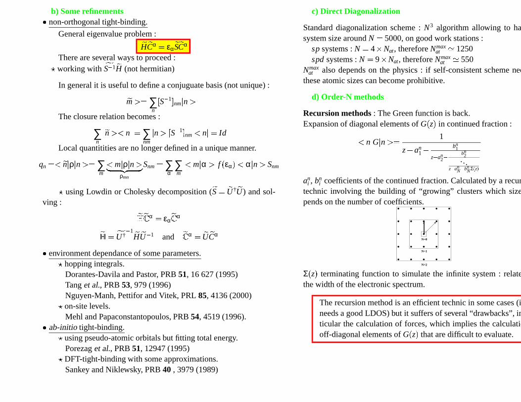
Recursion methods : The Green function is back.Expansion of diagonal elements of G

�

z

�

in continued fraction :

� n�

G�

n � � 1

z � an1

� bn1

z an2

bn2

...z � an

N

� bnNΣ

�

z

�

ani , bn

i coefficients of the continued fraction. Calculated by a recursiontechnic involving the building of “growing” clusters which size de-pends on the number of coefficients.

N=0

N=2

N=1

Σ

�

z

�

terminating function to simulate the infinite system : related tothe width of the electronic spectrum.

The recursion method is an efficient technic in some cases (if oneneeds a good LDOS) but it suffers of several “drawbacks”, in par-ticular the calculation of forces, which implies the calculation ofoff-diagonal elements of G

�

z

�

that are difficult to evaluate.

Fermi Operator expansion : The density operator is back.

� Chebyshev expansionFermi function in a Chebyshev polynomial expansion :

ρ � f

�

H

� � p

�

H

� � c0

2I

� npl

∑j � 1

c jTj

�

H

�

matrix recursion relations :����

��

T0

� �

H

� ��

I �

T1

� �

H

� �

�

H �

Tj

�

1

� �

H

� � 2

�

HTj

� �

H

� � Tj 1

� �

H

�

� rational representation

F � ∑ν

wν

H � zν

Contour integral :

f

�

ε

� � 12iπ

�

dzε � z

The discretization of this integral leads to :

f

�

ε

� �

npd

∑ν � 1

wν

ε � zν

occupied

ε

states states

unoccupied

integration path

energy

f( )

Decomposition of the energy

a) The band (bond) termOne important part of the total energy is the band energy term.

Eband

� 2∑α

f

�

εα

�

εα

��

E f

�

E

�

n�

E�

dE � Tr

�

ρH

�

Ebond

� 2∑n

��

E � ε0n

�

f

�

E�

nn�

E�

dE

E

ε0n(E)

R

Ebond is an attractive term.b) The repulsive term

Repulsive pairwise “empirical” potential :

Vrep

� ∑n

∑m

neighbour of n

Anme

p

� RnmR0

1

�

E coh

E bond

E coh E bondV

V

R

rep= +rep

Double couting terms to be substracted : Edc

� ∑n qnδVn

Ecoh

� Ebond

�

Vrep

� ∑n

qnδVn

c) A different approach

a problem of energy reference

Raising of the on-site levels in a “non-rigid” manner.

EdATOM

sp

n(E)

E

d

Ef

p

d

s

E

SOLID RThe “bonding” contribution of s and p electron is “unphysical”.

passing round the problem

Onsite levels are shifted in such a way that the cohesive energy is onlygiven by a band term : the repulsive term is “hidden” in the raising ofon site levels.

Ecoh

� ∑α

ε

�

α

On site levels are environment dependant :

ε0iλ

� aλ

�

bλg2

�

3i

�

cλg4

�

3i

�

dλg2i

gi

� ∑j

��� iexp

� � p

�

Ri j

�

R0

� 1

� �

fc

�

Ri j

�fitting the parameters

Parameters are obtained by a simultaneous fitting of band-structure andtotal energy.

FORCES

a) Derivative of the band term

Eband

� 2Tr

�

ρH

� 2∑nm

ρnmHmn

Derivation of Eband with respect to a displacement δrk :

dEband

drk

� 2

�

Tr

� dρdrk

H �

Tr

�

ρdHdrk

�

Or more explicitely :

dEband

drk� 2

�

∑nm

dρnm

drkHmn

�∑nm

ρnmdHmn

drk

�

The first term is very small :

dEband

drk

� 2Tr

�

ρdHdrk

b) Local charge neutrality is not a problem !

Local potential : δV � ∑n

�

n � δVn

� n

�

Eband

� Tr

� �

H0

� δV

�

ρ

�

H0

� δV

� � ∑n

qnδVn

� � �

Tr

�

ρ

�

H0

�δV

�

δV

�

� Tr

�

H0ρ

�

H0

� δV

the LCN potential δV does not appear explicitely. Therefore we have :

dEband

drk

� 2Tr

�

ρdH0

drk

c) Derivative of the repulsive term

The repulsive potential is a simple pair-interaction it is therefore im-mediate to derive analytically.

All terms of the Hamitonian Hnm have an analytical expression andforces are straightforward to calculate.

Empirical Potentials

a) Tight-Binding derived empirical potential

o

Ef

ε

� � � � � � � � � �

� � � � � � � � � �

� � � � � � � � � �

� � � � � � � � � �

� � � � � � � � � �

� � � � � � � � � �

� � � � � � � � � �

� � � � � � � � � �

� � � � � � � � � �

� � � � � � � � � �

� � � � � � � � � �

� � � � � � � � � �

g(x)

2l0 1 Ne

Ebond ∝ Wg

�

Ne

�

with W ∝

�

µ

�

2

�

g

�

x

�

parabolic-like function (whatever the DOS).

Second Moment potential :

Ebond

� ∑n

Enbond

Second moment approximation

Enbond ∝

�

µ

�

2

�

n

It leads to a potential of the form :

Etot

� � ∑n

∑m

��� nξ2

nme

2q

� RnmR0

1

� �∑n

∑m

��� nA2

nme

p

� RnmR0

1

�b) Embedded Atom Potentials

Etot

� ∑n

F

�

ρn

�

r

� � �

Vpair

�

r

�

Second moment potential is very similar to embedded atom potential(EAM) eventhough its justification is very different.

ρn

�

r

� � ∑m

��� nξ2

nme

2q

� RnmR0

1

�

F

�

ρ

� � �ρ

DFT justification

a) The DFT energy

E

�

ρ

� ∑α

fαεα

� � �

Tr

�

ρH

��

�

Ve f f

�

r

�

ρ

�

r

�

d3r

�

F

�

ρ

���������

�������

Ve f f

�

r

� � VN

�

r

� � � ρ

�

r

� �

�

r � r

� � d3r

�

� � �VH

�

r

�

�µxc

�

r

�

� � �

ddρ

�

ρεxc

�

ρ

� �

F

�

ρ

� 12

� � ρ

�

r

�

ρ

�

r

� �

�

r � r

� � d3rd3r

� �

VN

�

r

�

ρ

�

r

�

d3r

� �

εxc

�

ρ

�

r

� �

ρ

�

r

�

d3r

� �

Exc

�

ρ

�

EN N

Therefore it comes that :

E

�

ρ

� ∑α

fαεα � 12

� � ρ

�

r

�

ρ

�

r

� �

�

r � r

� � d3rd3r

� � ��

εxc �

r

��µxc �

r

� �

ρ

�

r

�

d3r

EN �N

Which can be written in a “condensed manner” :

E

�

ρ

� Tr

�

ρH

� Tr

�

ρ

�

1

�

2VH

�

µxc

� �

Exc

�

ρ

�

ENN

b) Kohn Sham algorithm

ρin

Ve f f

H

�

ψα

� � εα

�

ψα

�

ρout

E

�

ρin � ρout

�

�

ρout

� ρin

� � ε

c) Kohn-Sham and Harris energyEKS

�

ρin � ρout

� Tr

�

ρoutH

� Tr

�

ρout

�

1

�

2V inH

�

µxc

�

ρin

� � � �

Exc

�

ρout

�

ENN

EHar

�

ρin � ρout

� Tr

�

ρoutH

� Tr

�

ρin

�

1

�

2V inH

�

µxc

�

ρin

� � � �

Exc

�

ρin

�

ENN

At self consistency we haveρin

� ρout

� ρ and EKS

�

ρ

� EHarris

�

ρ

� E

�

ρ

d) the right input density

ρin

�

r

� � ∑n

ρatn

�

r

�

with ρatn

�

r

� � ρat

�

r � n

�

Which can be written as an operator :

ρin

� ∑n

�

nλ � qatnλ

� nλ

�

Where qatnλ is the atomic occupation of the orbital λ at site n.

Ionic and Hartree potentials are also superposition of atomic contribu-tions :

VN

� ∑m

V mN ; VH

� ∑n

V nH

� ∑n

� ρat

�

r

� � n

�

�

r � r

� � d3r

�

The energy can be decomposed in the following way :

E � Tr

� �

ρout

� ρin

�

H

� bond energy�

Tr∑n

ρatn

�

∑m

��� n1

�

2V mH

�

V mN

� �

ENN

� Ees

� �

Exc

�

ρin

� ∑n

Exc

�

ρatn

�

� ∆Exc

� ∑n

�

Trρatn

�

T

�

1

�

2V nH

�

V nN

� �

Exc

�

ρatn

�

� atomic energy

Ees electrostatic interaction between neutral atoms.Ees EXACTLY PAIR INTERACTION

∆Exc variation of exchange correlation energy from atom to solid.∆Exc APPROXIMATELY PAIR INTERACTION

Ecoh� Ebond

�

Vrep

Step energies and step-step interactions

F. Raouafi, C. Barreteau, D. Spanjaard, M.C. Desjonquères, To be pu-blished in Surf. Science (2001).

n0

n

(p-1+f) bo

bob

step (h’k’l’)

o

θ

f

terrace (hkl)

d

Step energies of 5 different geometriesSomorjai notations Miller indices f Edge geometry 2D unit cell

p(111)x(100) step A (p+1,p-1,p-1) 2/3 nn p odd : PRp even : CR

p(111)x(111) step B (p-2,p,p) 1/3 nn p odd : CRp even :PR

p(100)x(111) (1,1,2p-1) 1/2 nn CRp(100)x(010) (0,1,p-1) 0 nnn p odd : CR

p even :PRp(110)x(111) (2p-1,2p-1,1) 1/2 nn CR

Step-step interaction

2 3 4 5 6 7Number of atomic rows in the terrace

0.72

0.73

0.74

0.75

0.76

0.77

0.78

Step

ene

rgy

(eV

/ato

m)

p(100)x(010) Rhodium

2 3 4 5 6 70.38

0.39

0.40

Step

ene

rgy

(eV

/ato

m)

p(100)x(111) Rhodium

2 3 4 5 6 7Number of atomic rows in the terrace

0.49

0.50

0.51

0.52

0.53

0.54

0.55

p(100)x(010) Palladium

2 3 4 5 6 70.28

0.29

0.30

p(100)x(111) Palladium

(b)

(c)(d)

spd tight-binding for transition metalsApplication to surfaces and clusters

C. Barreteau, D. Spanjaard, M.C. Desjonquères, PRB 58, 9721 (1998).

δV � 0 (no Local Charge Neutrality)

−9.0

−6.0

−3.0

0.0

3.0

E−E

F(e

V)

Γ M K Γ

δV with Local Charge Neutrality

0.0 1.0 2.0 3.0−9.0

−6.0

−3.0

0.0

3.0

E−E

F (

eV)

Γ M K Γ

ΓM

K

ab-initio Plane wavesA. Eichler, J. Hafner, J. Furthmüller G.Kresse, Surf. Sci. 346,300(1996).

M K GammaGamma

-7.5

-5

-2.5

0

2.5

5

7.5

10

energy [eV]

Rh(111) surface-states (criterion 2)

M K Gamma

-7.5

-5

-2.5

0

2.5

5

7.5

10

energy [eV]

Rh(111) surface-states (criterion 2)

Coalescence of Single-Walled Carbon NanotubesM. Terrones, H. Terrones, F. Banhart, J.-C. Charlier, and P. M. AjayanScience May 19 2000 : 1226-1229.