introduction into stata iii: graphs and regressions
DESCRIPTION
Introduction into STATA III: Graphs and Regressions. Prof. Dr. Herbert Brücker University of Bamberg Seminar “Migration and the Labour Market” June 27, 2013. 1GRAPHS Present your data graphically - PowerPoint PPT PresentationTRANSCRIPT
Introduction into STATA III: Graphs and Regressions
Prof. Dr. Herbert Brücker
University of Bamberg
Seminar “Migration and the Labour Market”June 27, 2013
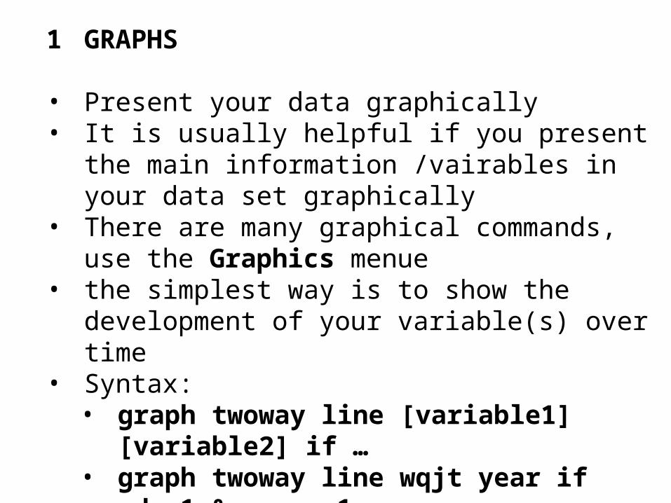
1 GRAPHS
• Present your data graphically• It is usually helpful if you present the main
information /vairables in your data set graphically• There are many graphical commands, use the
Graphics menue• the simplest way is to show the development of your
variable(s) over time• Syntax:
• graph twoway line [variable1] [variable2] if …• graph twoway line wqjt year if ed==1 & ex == 1
• This produces a two-dimensional variable with the wage on the vertical and the year on the horizontal axis for education group 1 and experience group 1
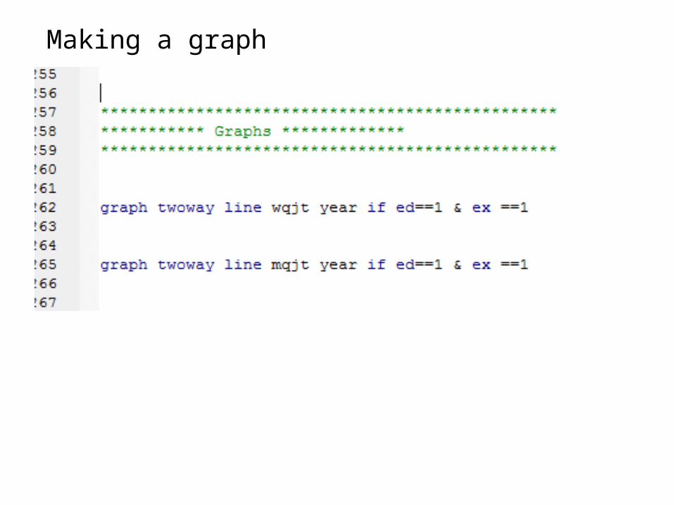
Making a graph
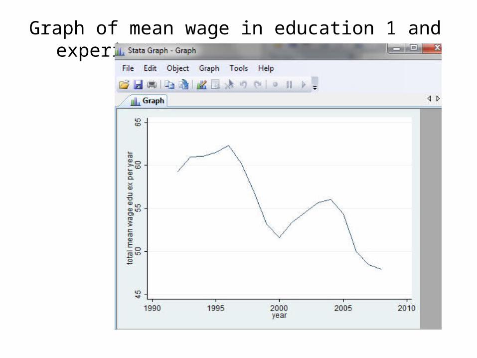
Graph of mean wage in education 1 and experience 1 group
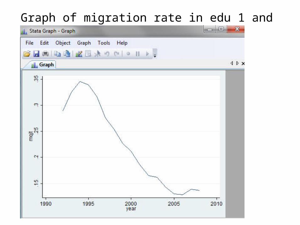
Graph of migration rate in edu 1 and exp 1 group
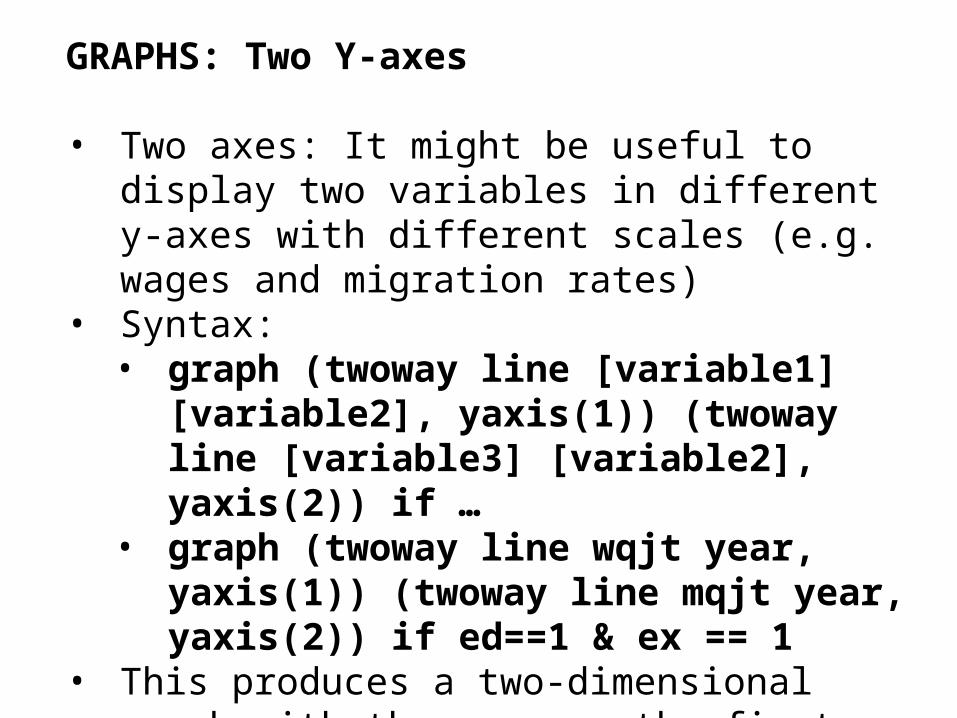
GRAPHS: Two Y-axes
• Two axes: It might be useful to display two variables in different y-axes with different scales (e.g. wages and migration rates)
• Syntax:• graph (twoway line [variable1] [variable2],
yaxis(1)) (twoway line [variable3] [variable2], yaxis(2)) if …
• graph (twoway line wqjt year, yaxis(1)) (twoway line mqjt year, yaxis(2)) if ed==1 & ex == 1
• This produces a two-dimensional graph with the wage on the first vertical axis (y1) and the migration rate on the second vertical axis (y2)
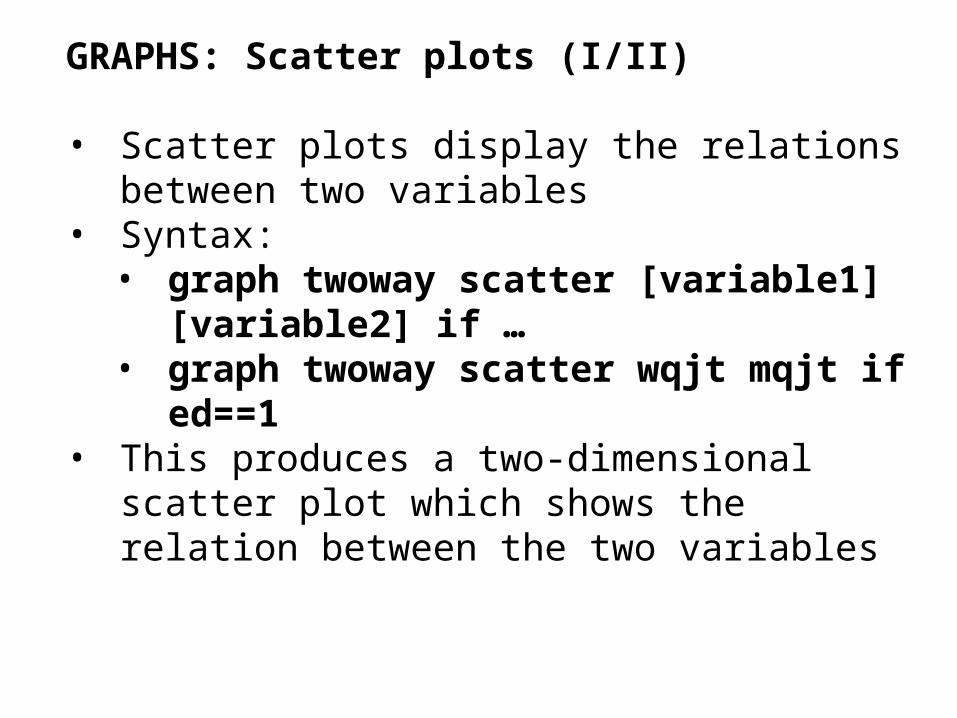
GRAPHS: Scatter plots (I/II)
• Scatter plots display the relations between two variables
• Syntax:• graph twoway scatter [variable1] [variable2] if …• graph twoway scatter wqjt mqjt if ed==1
• This produces a two-dimensional scatter plot which shows the relation between the two variables
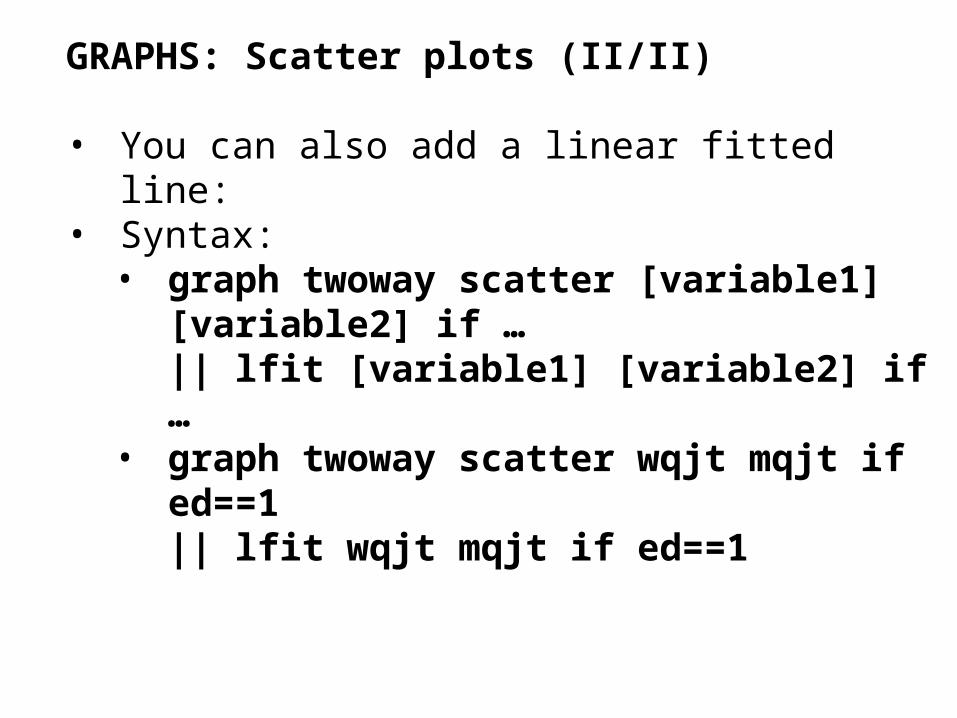
GRAPHS: Scatter plots (II/II)
• You can also add a linear fitted line:• Syntax:
• graph twoway scatter [variable1] [variable2] if …|| lfit [variable1] [variable2] if …
• graph twoway scatter wqjt mqjt if ed==1|| lfit wqjt mqjt if ed==1
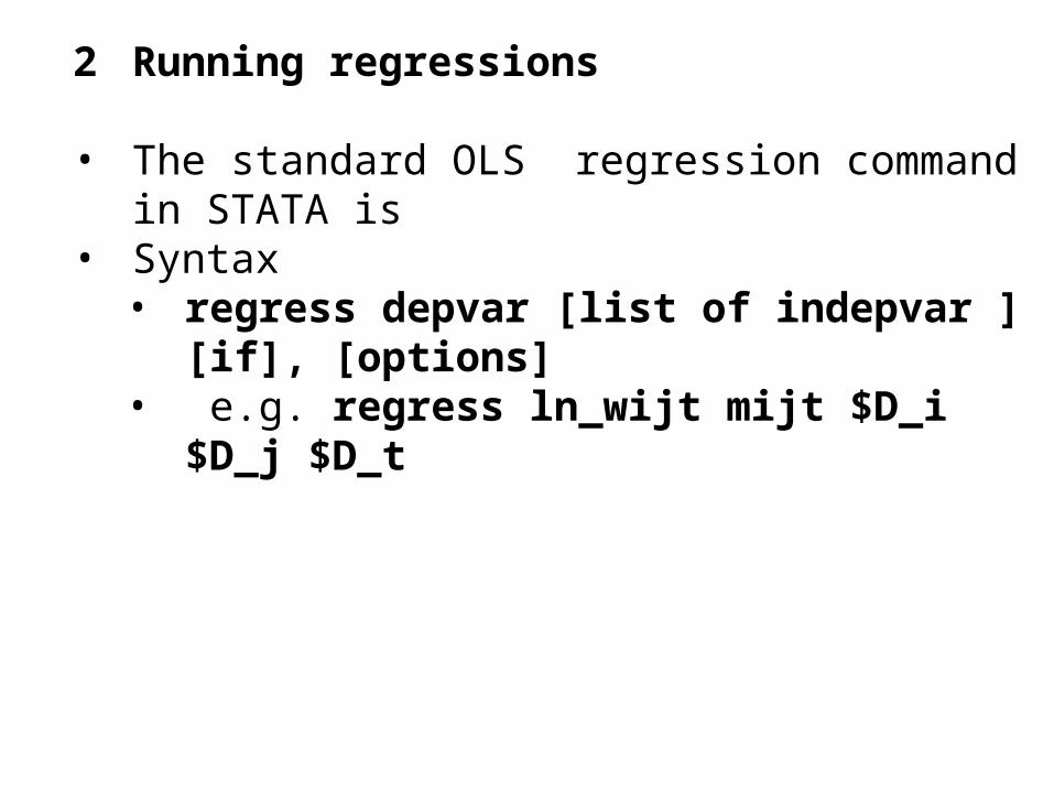
2 Running regressions
• The standard OLS regression command in STATA is• Syntax
• regress depvar [list of indepvar ] [if], [options] • e.g. regress ln_wijt mijt $D_i $D_j $D_t
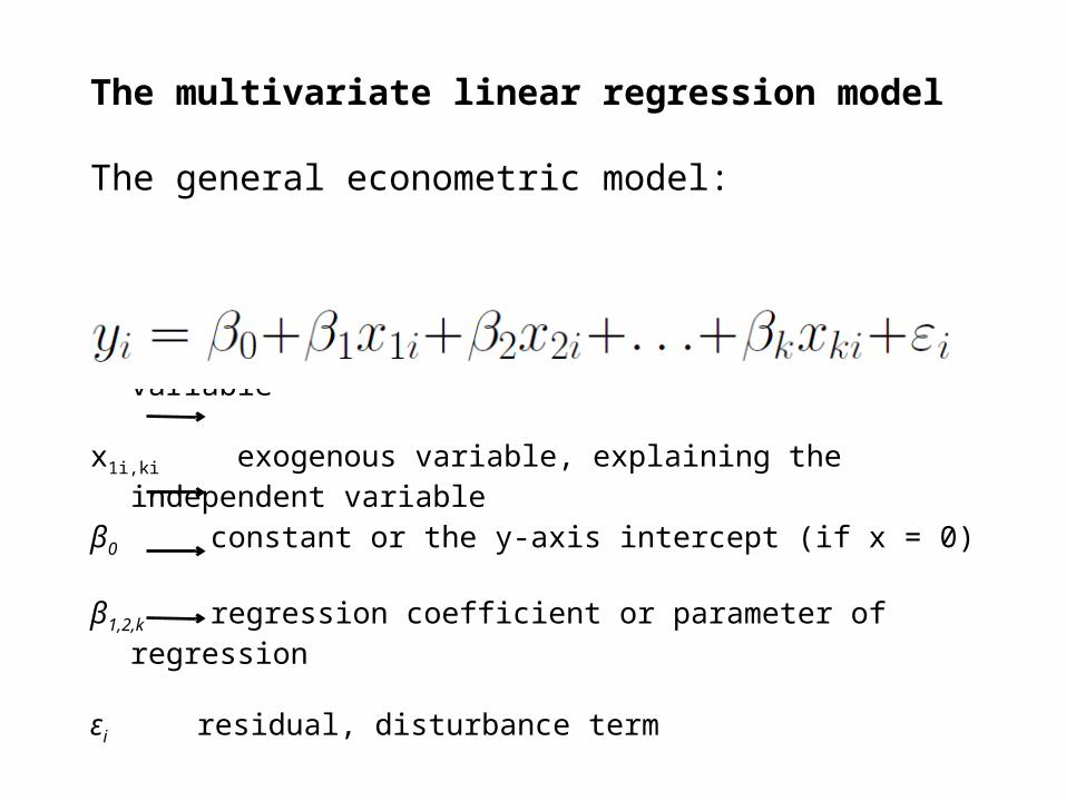
The multivariate linear regression model
The general econometric model:
γi indicates the dependent (or: endogenous) variable
x1i,ki exogenous variable, explaining the independent variable
β0 constant or the y-axis intercept (if x = 0)
β1,2,k regression coefficient or parameter of regression
εi residual, disturbance term
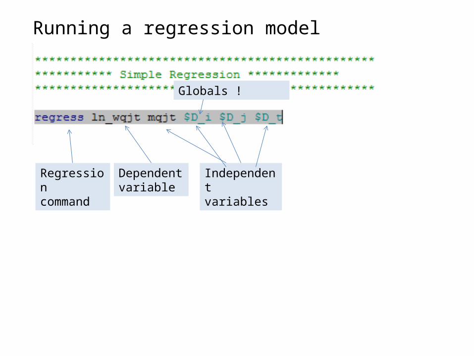
Running a regression model
Regressioncommand
Dependentvariable
Independentvariables
Globals !
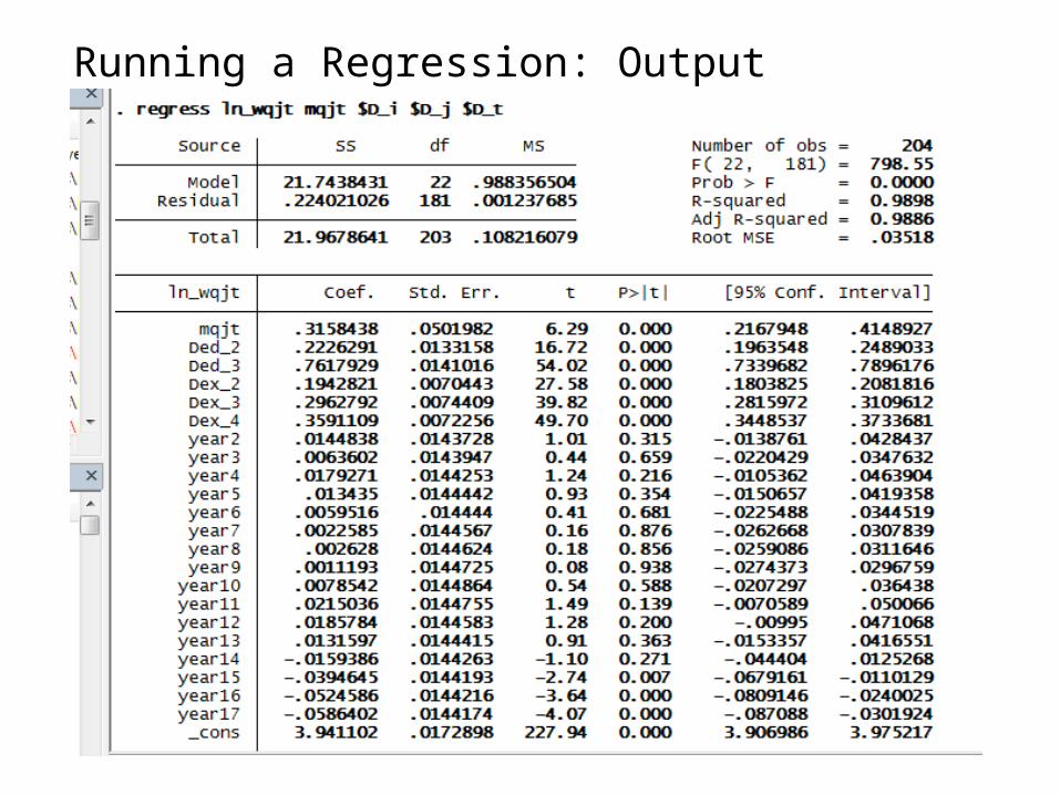
Running a Regression: Output
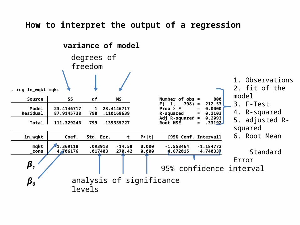
How to interpret the output of a regression
1. Observations2. fit of the model3. F-Test 4. R-squared5. adjusted R-squared6. Root Mean Standard Error
analysis of significance levels
variance of model
β0
β1
degrees offreedom
95% confidence interval
_cons 4.706176 .017403 270.42 0.000 4.672015 4.740337 mqkt -1.369118 .093913 -14.58 0.000 -1.553464 -1.184772 ln_wqkt Coef. Std. Err. t P>|t| [95% Conf. Interval]
Total 111.329246 799 .139335727 Root MSE = .33192 Adj R-squared = 0.2093 Residual 87.9145738 798 .110168639 R-squared = 0.2103 Model 23.4146717 1 23.4146717 Prob > F = 0.0000 F( 1, 798) = 212.53 Source SS df MS Number of obs = 800
. reg ln_wqkt mqkt
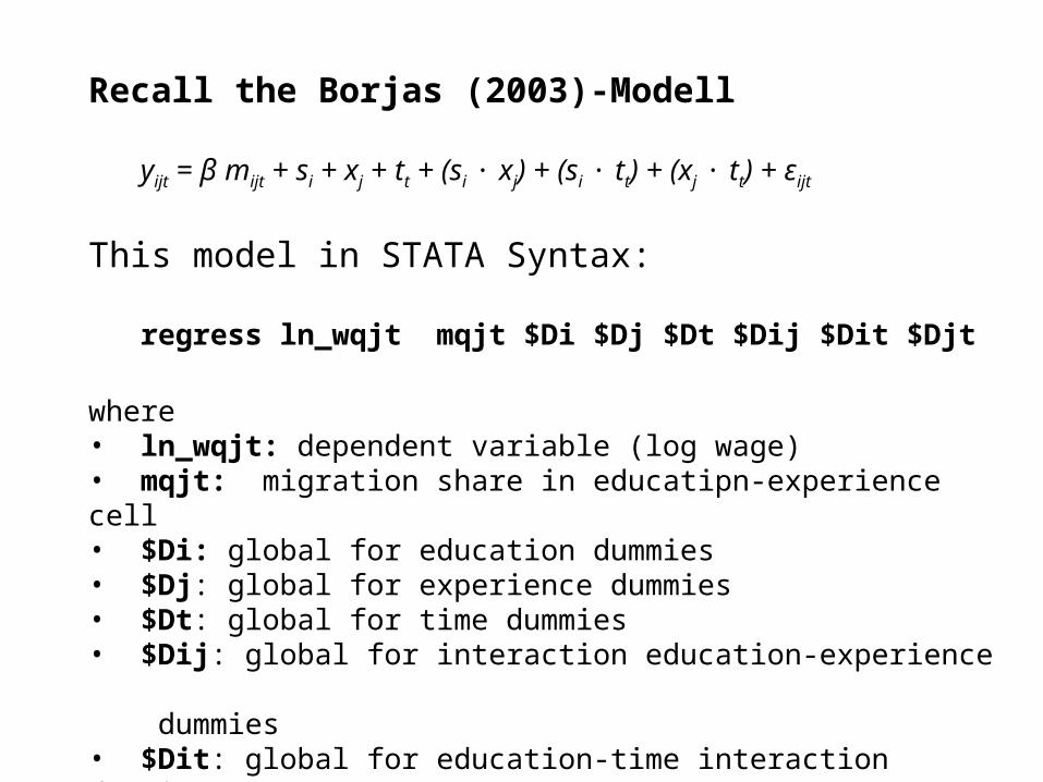
Recall the Borjas (2003)-Modell
yijt = β mijt + si + xj + tt + (si ∙ xj) + (si ∙ tt) + (xj ∙ tt) + εijt
This model in STATA Syntax:
regress ln_wqjt mqjt $Di $Dj $Dt $Dij $Dit $Djt
where• ln_wqjt: dependent variable (log wage)• mqjt: migration share in educatipn-experience cell• $Di: global for education dummies• $Dj: global for experience dummies• $Dt: global for time dummies• $Dij: global for interaction education-experience dummies• $Dit: global for education-time interaction dummies• $Djt: global for experience-time interaction dummies
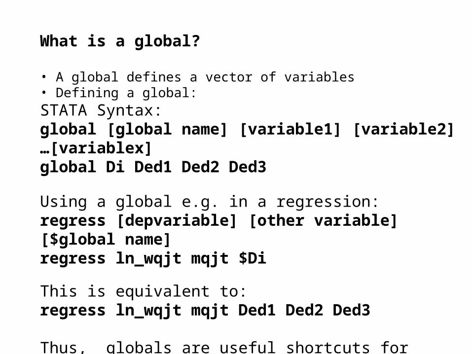
What is a global?
• A global defines a vector of variables• Defining a global: STATA Syntax:global [global name] [variable1] [variable2] …[variablex]global Di Ded1 Ded2 Ded3
Using a global e.g. in a regression:regress [depvariable] [other variable] [$global name]regress ln_wqjt mqjt $Di
This is equivalent to: regress ln_wqjt mqjt Ded1 Ded2 Ded3
Thus, globals are useful shortcuts for lists (vectors) of variables.
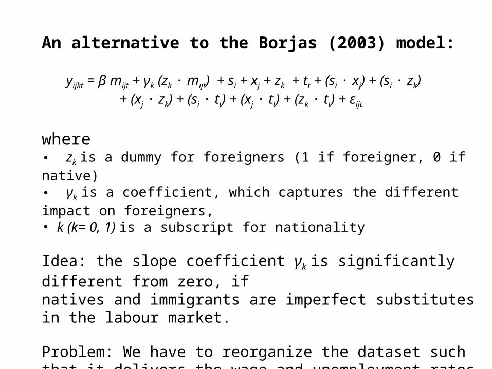
An alternative to the Borjas (2003) model:
yijkt = β mijt + γk (zk ∙ mijt) + si + xj + zk + tt + (si ∙ xj) + (si ∙ zk) + (xj ∙ zk) + (si ∙ tt) + (xj ∙ tt) + (zk ∙ tt) + εijt
where• zk is a dummy for foreigners (1 if foreigner, 0 if native)• γk is a coefficient, which captures the different impact on foreigners,• k (k= 0, 1) is a subscript for nationality
Idea: the slope coefficient γk is significantly different from zero, if natives and immigrants are imperfect substitutes in the labour market.
Problem: We have to reorganize the dataset such that it delivers the wage and unemployment rates etc. for foreigners and natives.
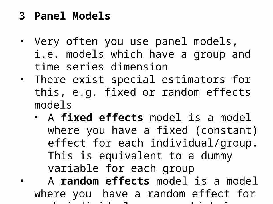
3 Panel Models
• Very often you use panel models, i.e. models which have a group and time series dimension
• There exist special estimators for this, e.g. fixed or random effects models• A fixed effects model is a model where you have a
fixed (constant) effect for each individual/group. This is equivalent to a dummy variable for each group
• A random effects model is a model where you have a random effect for each individual group, which is based on assumptions on the
distribution of individual effects
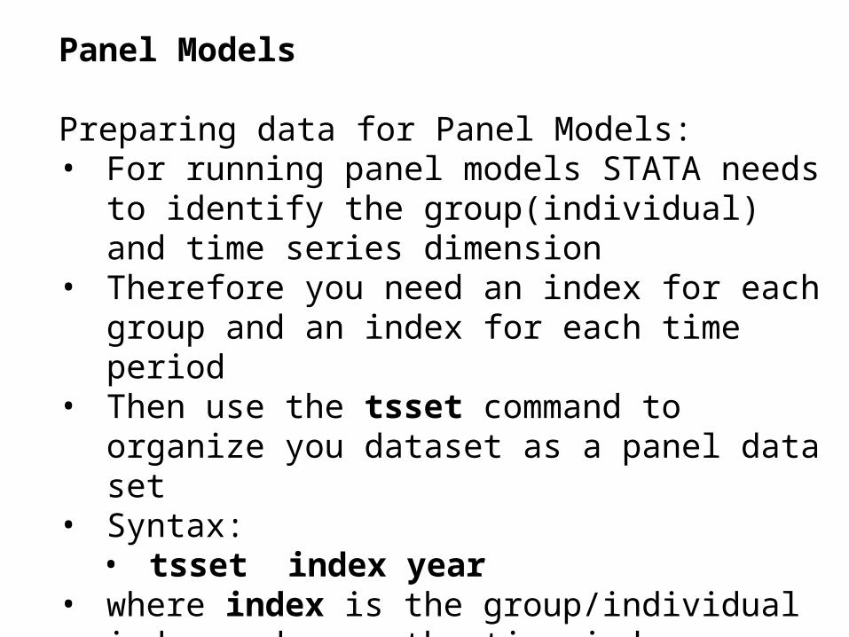
Panel Models
Preparing data for Panel Models:• For running panel models STATA needs to identify the
group(individual) and time series dimension• Therefore you need an index for each group and an
index for each time period• Then use the tsset command to organize you dataset
as a panel data set• Syntax:
• tsset index year• where index is the group/individual index and year
the time index
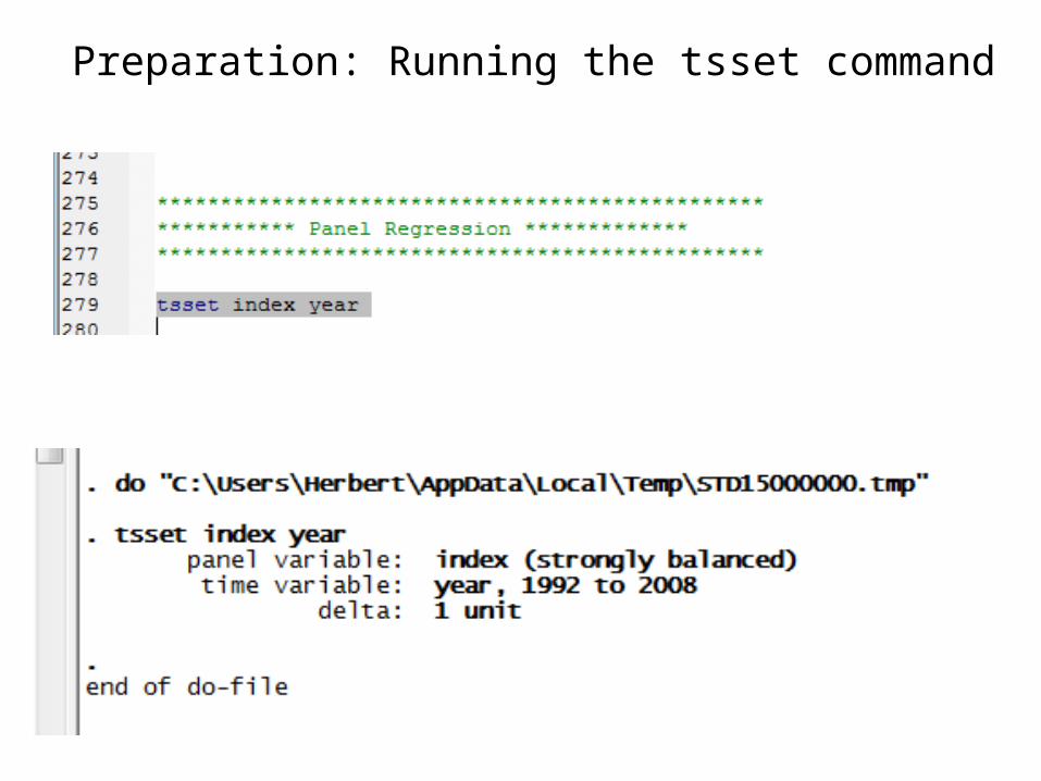
Preparation: Running the tsset command
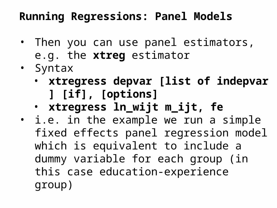
Running Regressions: Panel Models
• Then you can use panel estimators, e.g. the xtreg estimator
• Syntax• xtregress depvar [list of indepvar ] [if], [options] • xtregress ln_wijt m_ijt, fe
• i.e. in the example we run a simple fixed effects panel regression model which is equivalent to include a dummy variable for each group (in this case education-experience group)
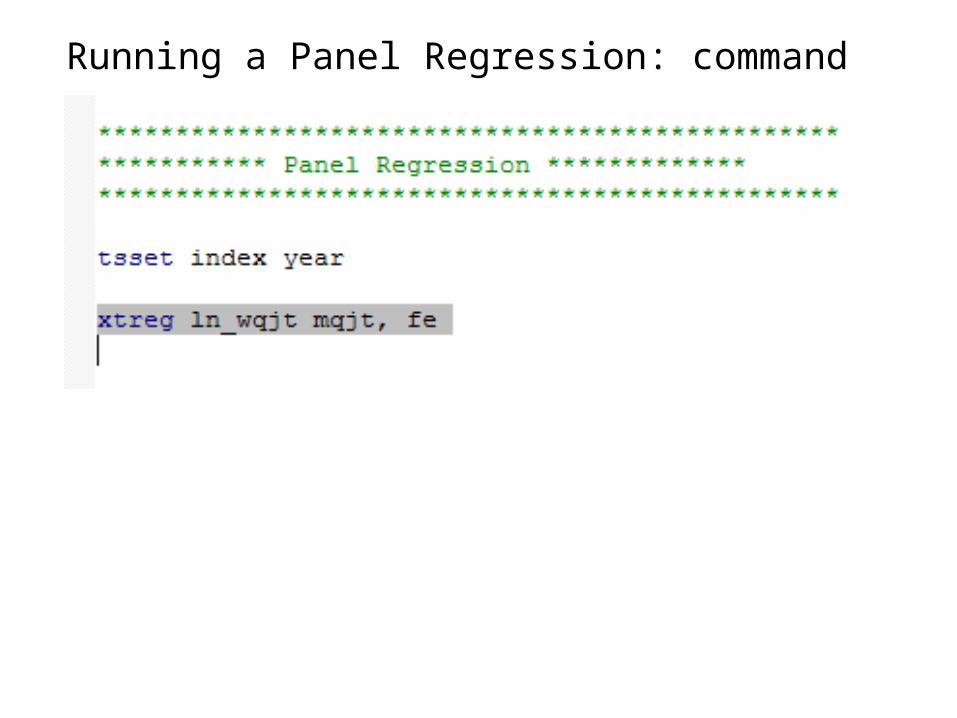
Running a Panel Regression: command
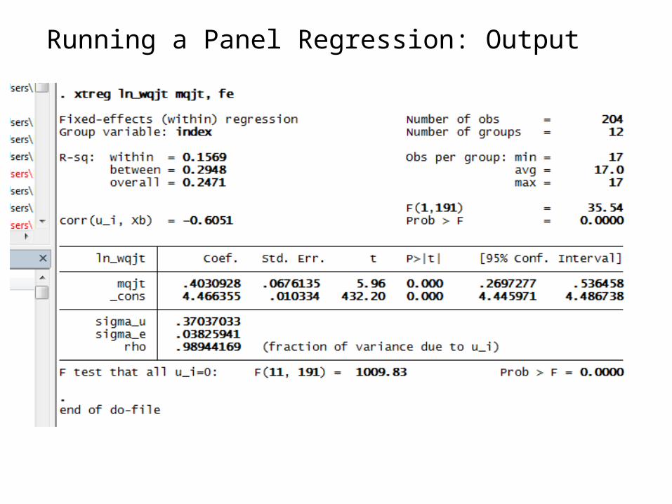
Running a Panel Regression: Output
Running Regressions: Panel Models
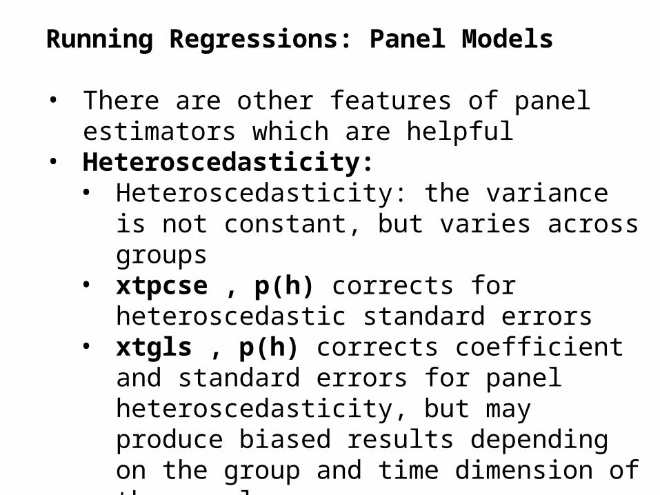
• There are other features of panel estimators which are helpful
• Heteroscedasticity:• Heteroscedasticity: the variance is not constant,
but varies across groups• xtpcse , p(h) corrects for heteroscedastic standard
errors• xtgls , p(h) corrects coefficient and standard
errors for panel heteroscedasticity, but may produce biased results depending on the group and time dimension of the panel
• Note: p(h) after the comma is a so-called “option” in the STATA syntax
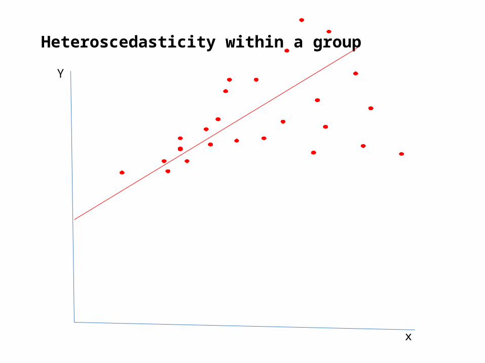
Heteroscedasticity within a group
Y
x
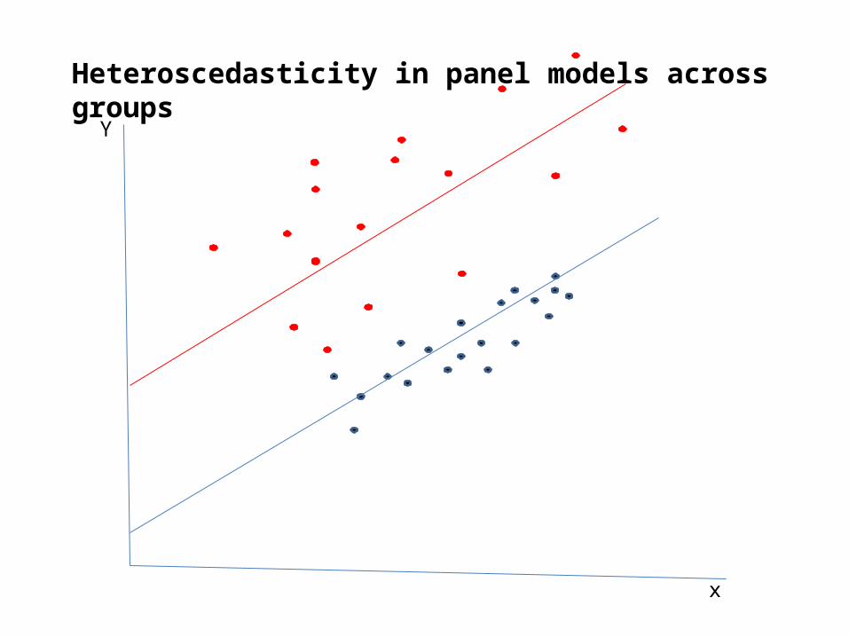
Heteroscedasticity in panel models across groups
Y
x
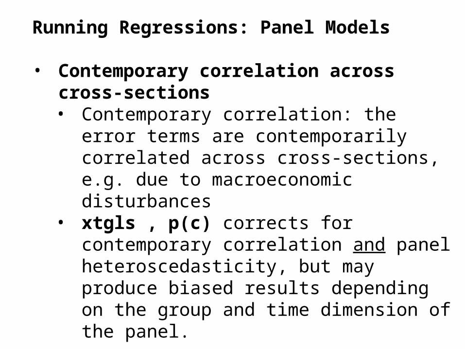
Running Regressions: Panel Models
• Contemporary correlation across cross-sections• Contemporary correlation: the error terms are
contemporarily correlated across cross-sections, e.g. due to macroeconomic disturbances
• xtgls , p(c) corrects for contemporary correlation and panel heteroscedasticity, but may produce biased results depending on the group and time dimension of the panel.
Next Meeting
July 4!
Presentation: July 18
Room RZ 01.02