introduction - mr mackenziemrmackenzie.co.uk/wp-content/uploads/2014/12/uncertainties_tcm4... ·...

PHYSICS 1

INTRODUCTION

The scope of this publication

This publication has been written for students and teachers involved inthe Higher Physics and Advanced Higher Physics courses. It is dividedinto three parts:

Part One (Sections 1–9) begins with a brief résumé of scientific notationand significant figures. This is followed by an explanation of whereuncertainties in experimental results come from. Then there isdescription of how to estimate the uncertainty in a measurement andhow to combine uncertainties in different measurements.

Part Two (Sections 10–15) deals with using graphs and spreadsheets toevaluate constants and quantify their uncertainties. Then follows asection on comparing the results of different experiments. There arenumerical examples throughout.

Part Three (Sections 16–21) explains briefly the theory of uncertaintiesand the various procedures described in Part One. It shows how to dealwith the uncertainties in functions and includes a short section onradioactivity measurements. It concludes by discussing the use ofcalculators for uncertainty calculations.

PHYSICS2

PHYSICS 3

PART ONE

1. Accuracy of measurements and uncertainties

Physicists are unable to measure quantities exactly and so it is importantto state explicitly the accuracy of a measurement.

The numerical result of any experiment should always be quoted as

value ± uncertainty

Experimenters can never determine the true value of a quantity becausethe accuracy with which a quantity can be established will always belimited by experimental error or uncertainty. However, the valuequoted should be the best estimate of the measurement or outcome ofthe experiment. The uncertainty gives a measure of how certain theexperimenter is that the true value is given by a value close to this bestestimate.

If the uncertainty is large, the true value may lie within only a largerange of the best estimate but if the uncertainty is small theexperimenter is claiming that the true value is close to the best estimate.The numerical result may be based on a single measurement, e.g. ameasurement of the length of an object using a ruler. In this case, thesmallest scale division marked on the ruler will give an indication of theuncertainty. Alternatively, the result may be obtained after combiningseveral measurements of this type. One then must know how tocombine the individual uncertainties. In other experiments, the valueand the uncertainty may require much analysis and the application ofadvanced statistical theory. In this case, the result will have a statisticalinterpretation and the range will indicate the probability of the trueresult lying within the limits given.

2. Significant figures and scientific notation

Significant figures

When calculating the result of an experiment or when quoting the resultof an experiment, one should always consider to how many digits theresult can justifiably be quoted.

UNCERTAINTIES: PART ONE

PHYSICS4

Numbers should be rounded to be compatible with the uncertainty inthe value, i.e. the number of significant figures quoted should match thedegree of certainty of the measurement or result. If numbers areexpressed in ‘scientific notation’, the digit before the decimal point isthe most significant digit and the last digit after the decimal point is theleast significant digit. This digit may be zero. More generally, the mostsignificant digit is the leftmost, non-zero digit in any number. If thenumber does not have a decimal point, and does not end in zero, thelast digit is the least significant one. If the number has no decimal pointand ends in one or more zeros then ambiguity could arise. The last zeromay or may not be the least significant digit. (See below.) If the numberdoes have a decimal point, the least significant is the last digit, even ifthis is zero. The number of significant figures is obtained by countingthe digits between the least and the most significant figure, includingboth of these. For example, each of the following numbers has foursignificant figures:

4.321 × 102

4.2100.0432143.2143,210

Ambiguities over trailing zeros (zeros at the right of a number notfollowed by any non-zero digit) can be eliminated by using scientificnotation. Express the number as one digit before a decimal point,followed by all necessary digits including the first uncertain one,followed by ten to the relevant power. (Better style would suggest thatthis rule be avoided where the power of ten is one of the following:–1, 0, +1.)

Note that a corollary of the above is that the last digit quoted in anumber should be interpreted as being uncertain, e.g. in the number2.15 × 103 the final 5 could be 4 or 6.

Determining which digit is the first uncertain digit is the substance ofwhat follows in this text.

For a fuller discussion of significant figures see references 11 and 12 (onpage 46).


PHYSICS 5

3. Uncertainties

In the content statements of the Higher Physics and the AdvancedHigher Physics and in this document, the use of the word ‘error’ islargely avoided although it is used extensively in the literature. Theword ‘error’ in this context is not synonymous with mistake or blunder;the word, where used, is in a scientific context and gives an estimate ofthe accuracy of the measurement or result of experiment. Uncertaintyconveys this more clearly and avoids possible misunderstanding; it isused here except when referring to systematic error and error bars. Ofcourse, mistakes and blunders are made by scientists but their effectscannot be quantified unless they are detected. Often, they can only bedetected by repeating the experiment and finding that one result isanomalous, e.g. one point on a straight line graph may be out of line, orby comparison of the result of one experimenter with that of another.

Reading uncertainty: The analogue scales on measuring instrumentscan only be read to some fraction of the smallest scale division. Oftenthis is taken to be ½ of the smallest division but it may be possible insome cases to estimate a smaller fraction reliably. The readinguncertainty for instruments with a digital scale would normally be takenas ±1 of the smallest change in reading.

Calibration uncertainty: The manufacturers of scientific instrumentscalibrate the instrument against approved standards and give anindication of the accuracy of this calibration. They give the accuracy ofcalibration in terms of a range within which any one of the instrumentsis expected to lie. For example, the maker of a steel ruler may state thatthe length of 1 metre on the scale of the ruler is accurate to ± 0.5 mm.Most of the instruments sold by the manufacturer will be correctlycalibrated or be very nearly correctly calibrated and large deviationsfrom the correct calibration will be unlikely, although it is possible thatwith age and use an instrument may deviate significantly from its originalcalibration.

Random uncertainty: If an experiment is repeated many times, theresult may not be the same each time. The experimenter may not set upthe apparatus in exactly the same way each time, may start or stop astopwatch with small differences of delay, etc. and these randomdifferences give a range of results. If the effects are truly random, theset of results can be analysed statistically and the best estimate and theuncertainty estimated.

Systematic effects: These are different from the others in that theyaffect all of the results of the experiment in the same direction, i.e. the


PHYSICS6

results are all too small or too large. A simple example would be ameasurement of length using a ruler. If the experimenter assumes thatthe zero of the scale coincides with the end of the ruler and it does not,then all the measurements will be too small. Alternatively, if the end ofthe ruler has been chopped off so that 5 mm is missing then allmeasurements will be too large. Of course, the experimenter shouldhave noticed that a mistake is being made and corrected for this error.However, not all systematic effects are as simple as this and it is usuallynot possible to detect or evaluate them. If a systematic effect exists inonly one of the variables being measured, then it may be possible todetect it using appropriate graphical treatment of the results – see page29.

4. Scientific notation, units and multiples of units

In formal scientific reports, numerical results are only given in terms ofthe SI units and a number of agreed additional units – metres, kilogramsand seconds being the most familiar. These units are listed in Appendix 1.It is convenient also to use multiples of these units and it isconventional to restrict these to multiples of 103 and denote these by aprefix to the unit. Strictly, this allows the metre, symbol m, themillimetre, mm, and the micrometre, etc. This does not allow for thecentimetre, cm. It is likely, however, that the centimetre will continue tobe used in all but the most formal of reports.

5. How uncertainties arise in experiments

Let us begin by looking at one particular experiment in some detail. Wecan suppose that Anne, a sixth-year student, is measuring theacceleration due to gravity, g, using a simple pendulum. She hangs thespherical metal bob by a cotton thread from a stand and measures thelength of this pendulum (from the point of support to the centre of thebob) with a wooden metre stick. Then she sets the pendulum swingingthrough a small angle and times ten oscillations with a digital stopwatch.She records her results:

length l = 51.25 cmtime for ten oscillations = 14.78 secondshence period t = 1.478 s.


PHYSICS 7

then, from the equation for the period of a simple pendulum,

she calculates her value of g to be 9.262 m s–2 (to 4 significant figures).

Now Anne cannot measure the length, l, with perfect accuracy. Firstly,she reckons that she can read the scale of the metre stick to the nearesthalf-division, that is to 0.5 mm, as each division is 1 mm. This is thereading uncertainty in the measurement. Secondly, when Anne checksher metre stick against a steel scale (more accurate and moreexpensive), she finds that it is about 0.5 mm too long, 1.0000 m on herruler corresponding to 0.9995 m on the steel scale.

This is a calibration uncertainty that will affect all measurements madewith the metre stick. If it is identified, as in this example, by comparingthe ruler with a steel rule, the measurements can be corrected for thiserror or deviation from the correct calibration.

It is reasonable to assume that her metre stick is uniformly too large andthat her readings of length should be multiplied by 0.9995 tocompensate. However, if the error is not identified, the error wouldstill affect the measurements – all measurements would be too large inthis case – and would be an example of a systematic effect. If themaximum value of the calibration uncertainty is quoted by themanufacturers, this value can be used as one of the uncertainties in theexperiment.

There are uncertainties too in the time measurement. The smallest timeinterval that the digital stopwatch can display is 0.01 seconds. This is itsreading uncertainty. (Anne cannot estimate to a fraction of a ‘timedivision’ as she can with the length division on the metre stick.) Again,when Anne checks her watch against the GMT time signals, she finds thatit is running about 1.5 seconds slow in 24 hours. This is its calibrationuncertainty; it is much less than the reading uncertainty, amounting toonly about 0.0002 seconds during Anne’s timing measurement and istherefore insignificant. This is another example of a systematic effectthat has been identified. The measurements could be adjustedaccordingly. Of course, if the GMT time signals are wrong (unlikely), herresults will be subject to the unknown systematic error that thisintroduces.

As neither of these uncertainties seems to be very large, Anne is leftwondering why her value for g is so much less than the value sheexpects, about 9.8 m s–2. She therefore takes two further pairs of

glT π2=


PHYSICS8

measurements, which we list together with her original pair:

length/cm time for 10 oscillations/seconds51.25 14.78 (original)51.40 14.3751.30 14.52

Let us look at the measurements of t first. They are spread over a rangeof about 0.4 seconds, which is much more than the readinguncertainties and the calibration error of the stopwatch. So there mustbe other uncertainties, coming not from the watch itself but from theway that Anne measures the times. She has, for instance, to judge whenthe pendulum is at the centre of its swing, and then to start and stop thewatch at the right moments. She can do none of these things precisely;she does them slightly differently each time. These and other randomeffects mean that her timings are all slightly different. We say that thereis an uncertainty caused by these random effects in her measurement oftime which, in this case, is larger than the reading uncertainty associatedwith a single reading of the stopwatch.

When Anne measures the length, l, she finds random effects there too.The metre stick is old and its ends are worn, so that the position of itszero mark is slightly uncertain. In addition, she has to estimate by eyewhere the centre of the spherical bob is in relation to the metre scale.Hence her measurement of length is also subject to uncertainty.

Now Anne can reduce these uncertainties by improving the experiment.If she uses a light beam and a photoelectric cell to detect when thependulum passes through its centre of oscillation, she can time theswings more accurately. She can use different lengths of thread and, byappropriate data handling, get round the problem of locating the centreof the bob. But she can never completely eliminate uncertainty.Vibrations and other disturbances, together with variations intemperature, pressure, humidity and so forth, will always prevent herobtaining exactly repeatable values of l and t. Hence although there issome ‘true value’ of g for Anne’s experiment, she can never find itprecisely!


PHYSICS 9

6. A closer look at uncertainty

Let us suppose now that Anne has set up a light beam and photoelectriccell so that she can time the oscillations more accurately. She thenobtains the following six values of g:

9.643 9.752 9.981 9.808 9.785 9.732 m s–2.

The spread of values here is due to the many random effects remainingin Anne’s experiment that are still beyond her control. What can she dowith these six different figures to improve the accuracy of her result?First, she takes the mean value of her results to be the best value of gthat she can obtain. (This may seem obvious but does in fact requireproof.)

mean value = (9.643 + 9.752 + 9.981 + 9.808 + 9.785 + 9.732)/6= 58.701/6 = 9.784 m s–2

She now wants to represent the uncertainty in this mean value by asingle figure. The simplest way to do this is to divide the range coveredby her six values (largest minus smallest) by six, the number of valuesthat she has measured.

This method works well for up to about 12 values (see, for example,reference 1 for more on this).

Thus: uncertainty ∆g = (9.981 – 9.643)/6 = 0.056 m s–2.

The mean value and the uncertainty can be written more compactly as:

g = 9.784 ± 0.056 m s–2.

How many significant figures should be used here? The uncertainty of0.056 m s–2 tells us that the true value of g probably lies somewherebetween 9.728 and 9.840 m s–2. ‘Probably’ here means a probability ofaround 70% (see Section 18 for details). Hence there is acorresponding probability of about 30% that the true value lies outsidethese limits. Moreover, further sets of measurements will yield differentmean values and different uncertainties.

Because the range only gives a statistical probability, the number ofsignificant figures justified in the uncertainty is limited; uncertainties


PHYSICS1 0

should usually be quoted to only one significant figure. However, inorder to avoid rounding uncertainties, it is best to do all calculations totwo significant figures until the final result is obtained. Then the finaluncertainty can be rounded off to one significant figure. (However, ifthat figure is a ‘1’, then the second figure should be retained). Themean value of the results should then be rounded off to an equivalentnumber of decimal places. Thus Anne would present the above resultas:

g = 9.78 ± 0.06 m s–2.

We now summarise the results of this section in algebraic form. For nvalues of a quantity x,

x1, x2, …, xi, …, xn,

the mean value x is given by

x = (x1 + x2 + … + xi + … + xn)/n = (6.1)

the range is (xmax – xmin) and the uncertainty ∆x is thus

∆x = (xmax

– xmin

)/ n (6.2)

7. Combining uncertainties

We have now identified three different types of uncertainty:

Calibration uncertainty – indicates how well an instrument has beenmade; see Appendix 2 for examples. If theinstrument can be compared with a moreaccurate measuring device, we cancompensate and remove this calibrationuncertainty from the results. If not, thisuncertainty remains as an unknownsystematic error.

Reading uncertainty – indicates how well an instrument scale can beread.

Random uncertainty – indicates the combined effect of all therandom factors affecting the experiment.


Σx i

n

PHYSICS 1 1

Ideally the experiment should be designed so that possible calibrationuncertainties are identified and so that both calibration and readinguncertainties are much smaller than the random uncertainty. Inpractice, this cannot always be done. Hence we need to know how toobtain from these three uncertainties a figure that represents the totaluncertainty in a measurement. The rule here is (see Section 8): Thesquare of the total uncertainty equals the sum of the squares of theindividual uncertainties.

Thus three uncertainties ∆x, ∆y and ∆z produce a total uncertainty ∆wgiven by

∆w2 = ∆x2 + ∆y2 + ∆z2. (7.1)

We use this expression when the three uncertainties are of comparablesize. If one uncertainty is about three or more times larger than theothers, then this uncertainty will dominate and it is not necessary tocarry out the calculation; we can take the total uncertainty to be thelargest uncertainty alone.

Thus, for example, suppose that ∆x = 1, ∆y = 3 and ∆z= 1. Then, usingequation 7.1, ∆w = √11 = 3.32. Rounding this to one significant figure(Section 3) gives ∆w = 3. Thus, to within the accuracy to whichuncertainties can be estimated, we have ∆w = ∆y.

This is a very important simplification. Whenever uncertainties arecombined by an equation such as 7.1, any uncertainty less than aboutone-third of the largest may be ignored. This often makes uncertaintycalculations much easier.

Example 7a

We measure the width w of a metal bar with a steel ruler and obtain theresult

w = 12.5 mm.

Calibration uncertainty = 0.1 mm (see Appendix 2)Reading uncertainty = 0.5 mm (our estimate)Random uncertainty = unknown, since it cannot be estimated from

one reading.


PHYSICS1 2

As the reading uncertainty is five times larger than the calibrationuncertainty, we take it alone as the total uncertainty, and write theresult as

w = 12.5 ± 0.5 mm

Example 7b

An analogue voltmeter, set to the 30 volt range, reads 17.5 volts. Thescale is marked in half-volt divisions. We estimate that we can read thisscale to one-fifth of a division, that is, to 0.1 volts.

Calibration uncertainty = 2% of 30 volts (Appendix 2)= 0.6 volts

Reading uncertainty = 0.1 voltsRandom uncertainty = unknown

Here the calibration uncertainty dominates and is taken to be the totaluncertainty; the result is:

voltage = 17.5 ± 0.6 volts

Example 7c

The temperature of the beaker of water is measured with a mercury-in-glass thermometer, marked in divisions of 1°C. The reading is 18.5°Cand the reading uncertainty is estimated as half a division.

Calibration uncertainty = 0.5°C (Appendix 2)Reading uncertainty = 0.5°CRandom uncertainty = unknown

As the calibration and reading uncertainties are of comparable size, weapply equation 7.1 and obtain for the total uncertainty:

We round this to one significant figure and give the result as:

Temperature = 18.5 ± 0.7°C

( ) ( ) 707.05.05.0 22 =+


PHYSICS 1 3

These three examples show how to estimate the uncertainties in singlereadings. However, it is always advisable to repeat measurements inorder to:

(i) detect blunders,(ii) check that the quantity being measured is not changing,(iii) estimate the uncertainty in the quantity being measured by

analysing the spread and distribution of the results obtained.

Example 7d

We measure the width of the metal bar (see example 7a) at six differentpoints down the length of the bar, again with the steel ruler. We obtain:

12.0, 12.5, 12.0, 12.0, 12.0, 12.0 mm

Calibration error = 0.1 mm (Appendix 2)Reading uncertainty = 0.5 mm (our estimate)

Here, the repeated value of 12.0 indicates that the uncertainty is sosmall that it is totally masked by the reading uncertainty. The only othervalue obtained differs by the reading uncertainty and so we concludethat the bar has parallel sides and take the best estimate of the width tobe the mean of the readings. We therefore take the reading uncertaintyto be the total uncertainty and give the result as:

w = 12.1 ± 0.5 mm

If we want more accurate values of w and ∆w, we will not get them bymore arithmetic, nor by further measurements of the same kind.Rather, we should reduce the reading uncertainty, either by reading thescale to less than 0.5 mm or by using a more accurate instrument, as inthe next example.

Example 7e

The width of the bar is now measured with vernier callipers, on whichthe scale can be read to the nearest 0.2 mm. Six values are obtained atdifferent points along the bar:

12.30, 12.22, 12.42, 12.56, 12.68, 12.54 mm.

Calibration uncertainty = 0.01 mm (Appendix 2)Reading uncertainty = 0.02 mmRandom uncertainty = 0.077 mm (using equation 6.2)


PHYSICS1 4

We take the random uncertainty alone as it is more than three timeslarger than either the calibration or the reading uncertainty. We expressit to one significant figure only, and the mean value (using equation 6.1)to the same number of decimal places. We write the result as:

w = 12.45 ± 0.08 mm

We should note that this result does not enable us to distinguishbetween random effects in the measurements and non-uniformity in thebar. If we feel that we are skilful enough to use the callipers to aboutthe same accuracy as the reading uncertainties, then we can attributethe uncertainty to non-uniformity. If we are not so confident, we mustmake repeated measurements at one point on the bar to discover howskilful we really are.

8. Uncertainty calculation

In most experiments, we enter our measured values into an equation inorder to calculate the final result. To find the uncertainty in this result,we have to combine the uncertainties in these values in some way. Thisusually requires us to be able to find:

(i) the uncertainty in a quantity raised to some power,(ii) the uncertainty in the product or quotient of two quantities,(iii) the uncertainty in the sum or difference of two quantities.

Let us first note that we can write the uncertainty in a quantity x inseveral ways, as the absolute uncertainty ∆x, or as the fractionaluncertainty ∆x/x, or expressed as a percentage, (∆x/x)×100 %.

8(i). The uncertainty in a quantity raised to a power

If the quantity x is raised to a power n, then the fractional uncertainty inxn is n times the fractional uncertainty in x, i.e. n (∆x/x).

Example 8a

Suppose x = 2.50 ± 0.12. Find the uncertainties in


y = x3 and z = 1√x

PHYSICS 1 5

We first find the fractional uncertainty in x;

(It is often helpful to handle fractional uncertainties as percentages.)We then have:

for y = x3, n = 3 for

= 4.8% × 3 = 14.4% = 4.8% × ½ = 2.4%

but y = 2.503 = 15.6 but z = = 0.781

hence ∆y = 14.4% of 15.6 hence ∆z = 2.4% of 0.781= 2.24 = 0.0187

Only when the calculation is finished do we round off to an appropriatenumber of significant figures (Section 2). We then write:

y = 16 ± 2 z = 0.781 ± 0.019

For negative n, we ignore the negative sign, as uncertainties are alwaysexpressed as plus-or-minus some number. Thus the fractionaluncertainty in 1/x (= x–1) equals the fractional uncertainty in x, eventhough their absolute uncertainties are different.

8(ii). The uncertainty in a product or quotient

Suppose two variables x and y are related by either w = xy or w = x/yIn each case the fractional uncertainty in z is given by

(8.1)

Example 8b

A voltage of 17.5 ± 0.6 volts (example 7b) is measured across a 560 Ωresistor marked with a gold band. The current through the resistor isthus 17.5/560 = 0.0313 amperes = 31.3 mA. Find the uncertainty in thisvalue.

% 8.4or 048.050.2

.12.0 ==∆xx

22

∆+

∆=∆

yy

xx

ww


∆yy

∆zz

1√2.5

1√x

z = , n = – 12

PHYSICS1 6

The fractional uncertainties are:

∆V/V = 0.6/17.5 = 0.034 or 3.4%∆R/R = 0.05 or 5% (see Appendix 2)

The fractional uncertainty in the current is then

Then, as 0.06 of 31.3 is 1.9, we may write the value of the current as

I = 31.3 ± 1.9 mA

As the first figure in the uncertainty is ‘1’ we give the uncertainty here totwo significant figures and express the current to a correspondingnumber of decimal places. Notice that we first calculate the twofractional uncertainties separately so that we can compare theirmagnitudes before combining them. If one of them is three or moretimes larger than the other, then (as in Section 7) we take the larger oneonly to be the total uncertainty. Alternatively we often compare %uncertainties, in this case 3.4% for voltage and 5% for resistance, to seeif any can be neglected.

This method can be extended to any number of quantities combined bymultiplication or division. Thus if w = (xy)/z, then

8(iii). The uncertainty in a sum or difference

If w is related to x and y by

w = x ± y

then the absolute uncertainty in w is given by

(8.2)

Example 8c

The temperature in a beaker of water rises from T1 = 18.5°C to

T2 = 22.0°C. Find the uncertainty, ∆T, in the temperature rise T2 – T1.

222

∆+

∆+

∆=∆

zz

yy

xx

ww

22 yxw ∆+∆=∆


(∆I/I) = √0.0342 + 0.052 = 0.06

PHYSICS 1 7

If, as in example 7e, the temperatures are measured with a mercury-in-glass thermometer, then T1 and T2 each have a reading uncertainty of0.5°C and a calibration uncertainty of 0.5°C. However, it is reasonable tosuppose that for a small temperature rise, the calibration uncertaintieswill largely cancel each other out. Hence we are left with the readinguncertainties alone so that:

T1 = 18.5 ± 0.5°C; T2 = 22.0 ± 0.5°CHence ∆T2 = (0.5)2 + (0.5)2 = 0.5 and ∆T = 0.7°C,so that T

2 – T

1 = 3.5 ± 0.7°C

Note here that the fractional uncertainty ∆T/T is made very large (20%)by the small temperature rise. This points to poor experimentalprocedure, which should be improved either to produce a largertemperature rise or to enable T1 and T2 to be measured more accurately.

Armed with the techniques of 8(i) – (iii), we can now find theuncertainties in more complex equations.

Example 8d

John is measuring the specific heat capacity c of a liquid. He immerses aheater of resistance R in a mass m of the liquid, and passes a current Ithrough it for t seconds. The temperature of the liquid rises from T1 toT

2. The energy output of the heater, I 2 R t, equals the energy gain of the

liquid, mc (T2 – T1). Hence

(8.3)

To find the uncertainty ∆c, John works as follows:

(i) he finds the fractional uncertainty in I2 (example 8a),(ii) he finds the absolute uncertainty in T

2 – T

1 (example 8c), and

converts it to a fractional uncertainty,(iii) he compares these two fractional uncertainties with those in R, m

and t, and discards all that are less than one-third of the largest,(iv) he combines the remaining fractional uncertainties (example 8b)

to give the fractional uncertainty in c,(v) finally, he converts this to an absolute uncertainty and presents the

result in the form c ± ∆c.


c =I2Rt

m(T2 – T1)

PHYSICS1 8

9. Graphical methods

In the last example (8d), John would be very unenterprising if he weresimply to measure the rise in temperature for just one period of time. Itwould be far better to read the thermometer at regular time intervalsand then plot a graph of temperature against time. This graph will be astraight line (if the liquid is well insulated). Its gradient will equal theaverage rate of temperature rise and will in effect be the average ofseveral pairs of temperature-time measurements. Hence it can replace(T2 – T1) / t in equation 8.3.

If John adopts this graphical method, he then faces the problem offinding the uncertainty in the gradient of a graph. We now see how todo this.

A straight-line graph has the general form

y = mx + b where b is the intercept.

In John’s experiment, the water temperature T is the dependent variablerepresented by y and the heating time t is the independent variablerepresented by x. Suppose that he obtains the following results:

t /min 0 5 10 15 20 25 30 35

T / 0C 18.0 26.0 27.5 30.0 36.0 46.5 50.0 54.0

We first plot the points in the usual way (Figure 1).

Figure 1


Temperature vs Time

-5.0

5.0

15.0

25.0

35.0

45.0

55.0

65.0

-10.0 0.0 10.0 20.0 30.0 40.0

Time (min)

Tem

pera

ture

(o C)

C

B

A

D

Time / min

Tem

pera

ture

/ º

C

PHYSICS 1 9

As the points are all of equal accuracy (reading uncertainties in t and Tbeing the same for all readings) then it can be shown that the beststraight line through them passes through their centroid. This is the‘centre of mass’ of the points; its co-ordinates are the means of all the xand y values. Here the centroid is the point (17.5, 36.0) and is markedwith a square.

We then draw what we judge to be the best straight line through thecentroid. When this is done by eye, our judgement will almost certainlybe based on minimising the deviations of the points from the line. Aswill be seen later, when the best straight line is calculated, it is the sumof the squares of the deviations that is minimised and not themagnitudes of the deviations. After drawing the line, the gradient andintercept, m and b, are found in the usual way:

m = 1.12°C/min; b = 16.3°C

We now enclose the points in a long thin box, a ‘parallelogram ofuncertainty’ (reference 3). The ends of the box are vertical lines AD andBC through the first and last points of the graph. The top line AB isdrawn parallel to the best line (this can be judged by eye – see later for amore reliable method using a spreadsheet program) so that it passesthrough the point that lies farthest above the best line – here it is thepoint (5, 26.0). The lower line DC is similarly drawn through the pointthat lies farthest below the best line – here it is the point (15, 30.0).

The ‘worst’ lines that could reasonably be drawn through the points arethe diagonals of the parallelogram, AC and BD. From the gradients ofthese diagonals we can find the uncertainty ∆m in the gradient of thebest line. It is better not to draw in the diagonals, as the graph thenbecomes very cluttered. We just need the co-ordinates of the corners ofthe parallelogram. They are:

A, (0, 20.0) B, (35, 60.0)C, (35, 52.0) D, (0, 13.0)

The gradients of the two diagonals are:

m(AC) = 0.91 m(BD) = 1.34.

Then, for n points on the graph, the uncertainty in m is given by:

so that: m = 1.12 ± 0.09°C/min

088.062

43.0)2(2

)()( ==−

−=∆n

ACmBDmm


PHYSICS2 0

The fractional uncertainty ∆m/m is then 0.09/1.12 = 0.08, and thepercentage uncertainty is 8%.

The factor 2 in the expression for ∆m arises because the best line bisects(roughly) the angle between the two diagonals. The factor ( )2−ncomes from the statistical theory of the best line. We see that increasingthe number of points reduces the uncertainty in the gradient, as wewould expect.

If the uncertainty ∆b in b is required, we can find it in a similar way. Thediagonals AC and BD are extended back to the y-axis (not necessary inthis example, as A and D are already on the y-axis) and the twointercepts found. Here they are b(A) = 20.0 and b(D) = 13.0. Then ∆bis given by

Hence: b = 16.3 ± 1.6°C

If all we want is the fractional uncertainty in the gradient, ∆m/m, thenwe can use a quicker method. Suppose we use the horizontal distancebetween the verticals AD and BC to find all three gradients m, m(BD)and m(AC). Then, from the geometry of Figure 1, we have:

Using the co-ordinates of the corners, we have

The fractional uncertainty in m is 8% as before.

Using this method, we do not even have to measure y(A), y(B) and y(C)in units of y; we can simply count millimetres up the graph paper.

08.06

10.40

86

10.2060

5260 =×=×−−=∆

mm

)2(21)()(−

×−

=∆nm

ACmBDmmm

)2(212−

××=∆nBA

BCmm

)2(21

)()()()(

−×

−−=∆

nAyByCyBy

mm


( ) – ( ) 72 ( – 2) 2 6b A b Db

n∆ = =

PHYSICS 2 1

Example 9a

John repeats his experiment (example 8d), using a graphical method toobtain the rate of temperature rise as a gradient, m degrees per second.Then the specific heat capacity of the liquid is

To find the uncertainty in c, John works as follows:

(i) he finds the fractional uncertainty in I 2,

(ii) he finds the fractional uncertainty in the gradient ∆m/m,(iii) he compares all the fractional uncertainties and discards as before,(iv) he combines the remaining fractional uncertainties to obtain ∆c/c,(v) he calculates the absolute uncertainty ∆c.

Suppose a single ‘rogue’ point lies a long way from the best line.Should it be included in the parallelogram or not? Such points are oftenproduced by misplotting; hence this should be checked first. Then theactual values of x and y should be examined and any obvious blundercorrected. If the point survives these tests, it should still be discarded ifit produces a parallelogram whose diagonals miss the centroid by asubstantial amount.

It is often helpful to show the reading uncertainties in x and y byplotting error bars on the graph. They can often give a ‘visual clue’ as tohow well the experiment has gone.

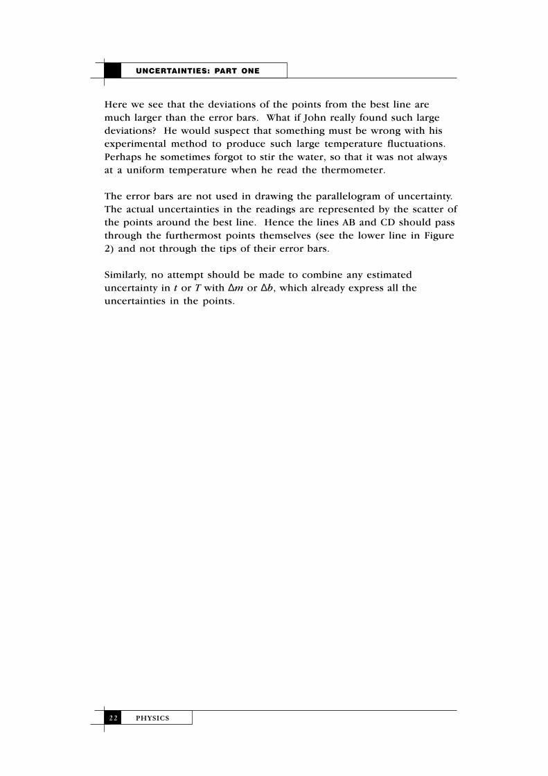
In John’s experiment, the reading uncertainty in the time t is too smallto show. The reading uncertainty in the temperature T is ± 0.5°C and isshown for three points in the enlarged central portion of the graph(Figure 2).

Figure 2


2I RcMm

=

2 6 .0

2 8 .0

3 0 .0

3 2 .0

3 4 .0

3 6 .0

3 8 .0

10.0

11.0

12.0

13.0

14.0

15.0

16.0

17.0

18.0

19.0

20.0

Time (min)

T/ o C

Time / min

PHYSICS2 2

Here we see that the deviations of the points from the best line aremuch larger than the error bars. What if John really found such largedeviations? He would suspect that something must be wrong with hisexperimental method to produce such large temperature fluctuations.Perhaps he sometimes forgot to stir the water, so that it was not alwaysat a uniform temperature when he read the thermometer.

The error bars are not used in drawing the parallelogram of uncertainty.The actual uncertainties in the readings are represented by the scatter ofthe points around the best line. Hence the lines AB and CD should passthrough the furthermost points themselves (see the lower line in Figure2) and not through the tips of their error bars.

Similarly, no attempt should be made to combine any estimateduncertainty in t or T with ∆m or ∆b, which already express all theuncertainties in the points.


PHYSICS 2 3

PART TWO

10. Use of graphs and spreadsheets

A graph is valuable as it provides a visual impression of the data.

• the existence or not of a trend is easily seen• points which do not conform to the general trend are readily

identified• the equation to which a set of data conforms may be suggested by the

distribution of the plotted points• spreadsheet programs allow graphs to be drawn and data analysed

with relative ease• by including error-bars, an impression can be got of the relative sizes

of random uncertainties, from the spread of the points, and of theother sources of uncertainty

It is always worth while drawing a graph of the results whilst theexperiment is in progress. Any point not conforming to the trend can beidentified and re-assessed, either by immediately re-doing themeasurement, or if this is not possible due to the experimentalconditions, then by re-doing that measurement before the equipment isdismantled. Care must be taken not to replace data unless one is certainthat the previous data was in error – if not, one is in danger of simplyconfirming one’s prior assumptions about the outcome of theexperiment.

The HSDU publication Physics Guide to Excel (reference 4) gives anexcellent introduction to setting up and using a spreadsheet to analyseexperimental results.

Before using the spreadsheet to draw a graph, some thought should begiven to the experiment being performed. The student should first of allassess whether the results are likely to fit a known relationship.Examples would be an experiment designed to investigate the pressure–volume relationship for a fixed mass of gas at constant temperature orone to investigate the inverse square law for gamma radiation.Frequently the results will be expected to conform to an equation, suchas that between the period of a pendulum and the length of thependulum. In this case constants will be involved, such as theacceleration due to gravity, g, and indeed it may be measurement of thisquantity that is the desired outcome of the experiment. Since a straight-line graph is immediately recognisable, the data in these cases should be

UNCERTAINTIES: PART TWO

PHYSICS2 4

handled in a way which would be expected to yield a straight line. Lesscommonly, the experiment may be designed to study some completelyunknown (to the student at least) relationship, such as that between theviscosity of a liquid and the quantity of some additive. In these cases noconstant is being measured, and any graph drawn will simply illustratethe trend.

11. Graphing results with the EXCEL spreadsheet – Adding atrendline and equation

The HSDU publication Physics Guide to Excel (reference 4) provides aclear, step-by-step account of how to produce a chart of a set ofexperimental points using an Excel spreadsheet. That guide alsoexplains how to add error bars to the plotted points. It does notexplain how to add a trendline and equation to the computer generatedchart.

After preparing the chart of the temperature readings versus time (seeFigure 3), proceed as follows –

• select the chart area in the spreadsheet by clicking on it once,• go to Chart on the Menu bar,• click on Add Trendline.• select Type – Linear• now click on the Options tab and tick the box Display equation on

chart

The least squares, best-fit line will be added to the set of plotted points.The equation of this line (given normally by y = mx + c but in EXCEL byy = mx + b) is given also. By double clicking on the best-fit line, thecharacteristics of the line, colour and weight can be altered; if desired, theline can be constrained to pass through a known intercept, by clicking onOptions, ticking the ‘set intercept’ box and specifying the intercept valuein the ‘=’ box.


PHYSICS 2 5

Figure 3

The equation of the best-fit line gives

m = 1.04 0C/ min; b = 17.88 0C

12. Uncertainties in gradient and intercept

Using a spreadsheet, the parallelogram (see Section 9, page 19) can beadded using the DRAW package. A line is drawn lying over the trendline,extending between the first and last ‘x’ values. By copying this line(CTRL C followed by CTRL V) a second identical line is generated.These lines can then be moved until they pass through the mostextreme upper and lower data points. Often these lines can be movedusing the keyboard direction arrows. For finer steps CTRL + ARROWcan be used. Finer grid-lines can be used to give the co-ordinates of thevertices of the parallelogram so formed.

13. Note on LINEST

It is straightforward to have the analysis package of the spreadsheet findthe values of the ‘standard error’ or ‘standard deviation’ of thegradient, and the ‘standard error’ (‘standard deviation’) of theintercept. (Note that in EXCEL the intercept is referred to by thesymbol ‘b’ rather than ‘c’). The function LINEST will supply thenecessary statistics. The example here uses the temperature–timereadings of the ‘heating water’ experiment:

t /min 0 5 10 15 20 25 30 35

T /0C 18.0 26.0 27.5 30.0 36.0 46.5 50.0 54.0


Temperature vs Time

y = 1.0357x + 17.875

-5.0

5.0

15.0

25.0

35.0

45.0

55.0

65.0

-10.0 0.0 10.0 20.0 30.0 40.0

Time (min)

Tem

pera

ture

(oC

)

Time / min

Tem

pera

ture

/ º

C

Temperature vs Time

PHYSICS2 6

The data are entered in the first two columns of an EXCEL spreadsheetas before, and the graph drawn, with a trendline inserted. The equationof the line can be shown on the chart by selecting – Chart Options –Insert Trendline, Options – tick ‘Display equation on Chart’ box.

Figure 4

As above (Figure 4), this gives a gradient of 1.04, and an intercept b of17.88.

When the statistics of the line are found they will be fitted into an array.Highlight a block of cells two columns wide by 2 deep, to take this data.With these cells highlighted enter the formula =LINEST. The dialog boxshown will open up:

Figure 5


Temperature vs Time

y = 1.0357x + 17.875

-5.0

5.0

15.0

25.0

35.0

45.0

55.0

65.0

-10.0 0.0 10.0 20.0 30.0 40.0

Time (min)

Tem

pera

ture

(oC

)

Time / min

Tem

pera

ture

/ º

C

PHYSICS 2 7

Click on the red symbol to the right of the first box (Known y’s) andenter the range of cells containing the y-values. This is most easily doneby running the cursor down column B from B2 to B9, or simply typethese cell references by hand. Do the same for the known x’s. Enter‘TRUE’ in each of the bottom two lines. To enter this formula as anarray, hold down CTRL + SHIFT and press ENTER at the same time.The formula should appear in the formula bar with brackets aroundit, and the cells you highlighted should now hold the desired data.

Figure 6

The top left cell which you highlighted contains m, and the top right cellcontains b. The standard deviation of each is the box immediately belowit.

In the screen display above, the names etc have been added to thesurrounding boxes. The program will not do this for you.

An alternative method is to highlight cells as described earlier, and thentype =LINEST() in the formula line. Place the insertion point inside thebrackets, then highlight the cells containing the y-data readings (in thiscase B2:B9), or simply enter these references, followed by a comma,then the range of the x-data (A2: A9), then a comma followed by TRUE,then another comma followed again by TRUE, giving =LINEST(B2:B9,A2:A9,TRUE,TRUE)


PHYSICS2 8

Now hold down CTRL + SHIFT and press ENTER. This should returnthe required values as before.

14. Data handling with a spreadsheet – seeking a straight line

Should a straight line relationship be sought, the spreadsheet makescalculations related to this extremely quick and easy to carry out.

Let us suppose that an experiment investigating the relationshipbetween the pressure and volume of fixed mass of gas yields thefollowing values of p and V. Reasonable care has been taken overcontrolling the temperature and mass of the gas:

Pressure p/ 10 5 Pa 1.00 1.09 1.20 1.33 1.50 1.71 2.00 2.40

Volume V/ cm 3 100 90 80 70 60 50 40 30

The student plots p vs 1/V, expecting a straight line:

Figure 7

The line on the graph was drawn through the first four points.

The result is clearly not what was expected, and should give cause forsome thought. The trend is getting further from a straight line for large1/V, i.e. for small V.

This could be because the assumed relationship pV = constant isincorrect, but alternatively there could be a systematic error in theresults. For example, a ‘dead-space’ in the equipment could cause allthe volume readings to be too small by the same amount.


p vs 1/V (uncorrected)

0

0.5

1

1.5

2

2.5

3

0.000 0.005 0.010 0.015 0.020 0.025 0.030 0.035

1/Volume (cm-3)

pres

sure

(Pa

x 1

05 )

(1/Volume) / cm–3

pres

sure

/ (

105

Pa)

PHYSICS 2 9

A plot is made of 1/p vs V in order to examine this possibility:

Figure 8

This shows clearly the offset in the volume, which is identified with adead-space in the equipment. In this case there was a dead-space of 20cm3. The apparatus may be redesigned to reduce or eliminate this. Theresults can be corrected to allow for the dead-space, and the linearrelationship can be shown to hold:

Pressure p/ 10 5 Pa 1.00 1.09 1.20 1.33 1.50 1.71 2.00 2.40

Volume V/ cm 3 100 90 80 70 60 50 40 30

CorrectedVolume 120 110 100 90 80 70 60 50/ cm 3

The equation is now that of a straight line through the origin, with nooffset.

The ease with which such graphs can be generated makes it possible toscrutinise data more closely when linearity is expected (and fails to showup). Examples where offsets are likely to occur are in the recording ofgas volumes – ‘dead-spaces’ as exemplified above, distances between alight-source and a detector, distances between a source of radiation anda geiger-tube, and so on. In fact, rather than attempt to measure from atrue zero, it may be more convenient and yield better data todeliberately introduce an offset. It is, for example, more straightforward,in a pendulum experiment, to mark the string above the bob and


1/p vs V for a gas (T constant)

-0.2

0.00.2

0.4

0.6

0.81.0

1.2

-20 0 20 40 60 80 100

V / cm3

(1/p

) / (1

05 Pa)

Voffset

PHYSICS3 0

measure from there. Length should then be plotted as the independentvariable, and the square of the period should be plotted as thedependent variable. In this case, the offset could be found from thegraph. If g is being measured, the offset is irrelevant, as g can beobtained from the gradient.

Note: This method will fail if there is an unknown systematic error inthe measurement of the dependent variable as well.

15. Comparisons of results

Once we have a numerical result in the form x ± ∆x, we can compare itwith the results of other experiments. As an example, let us compareAnne’s value for g with three other values, two obtained with apendulum and one with a spiral spring. The four results are listedbelow and shown in Figure 9 with the uncertainties drawn as horizontalbands.

R1 Pendulum 9.78 ± 0.06 m s–2 (Anne’s result)R2 Pendulum 9.88 ± 0.05 m s–2

R3 Pendulum 9.56 ± 0.07 m s–2

R4 Spring 9.6 ± 0.4 m s–2

Let us first look at these results on their own, disregarding whateverelse we know about the value of g. Figure 9 shows that R1 and R2 haveoverlapping error bands. Hence we can say that R1 is in goodagreement with R2. R3 lies somewhat lower and so is in rather pooragreement with R1 and R2.

Figure 9

R4

R3 R2

R1

9.0 9.2 9.4 9.6 9.8 10.0


PHYSICS 3 1

The uncertainty band for R4 encompasses all the others. Hence R4 is ingood agreement with R1 – R3, but its broad uncertainty band marksdown the spiral spring as a poor way of measuring g. By comparinguncertainties in this way, we can judge between one experimentalmethod and another.

The value of g used in SQA examination question papers is often givenas 9.8 m s–2. This is not the ‘right answer’ but rather a ‘generallyaccepted value’, derived from many careful experiments that haveproduced results with overlapping uncertainty bands that are very small.More comprehensive data books (for example, reference 7) reveal thatvery few of the so-called ‘constants’ are actually constant; most of themdepend on other physical parameters. Thus g varies with both latitudeand altitude (see reference 8). Across Scotland, at sea level, it rangesfrom 9.815 m s–2 in Stranraer to 9.819 m s–2 in Lerwick (withuncertainties less than 0.001 m s–2 in each value.)

As the uncertainty band for R1 includes these values, we say that R1 is ingood agreement with the generally accepted values of g for Scotland.The same is true for R2, for the lower edge of its uncertainty band(9.83 m s–2) is also very close to the accepted values.

There is however, a sizeable gap between the uncertainty band for R3and the accepted values; the agreement is poor. Perhaps there wassome undetected error in this experiment that displaced the result to alower value. However, we cannot be sure and so cannot say that R3 is‘wrong’. Instead we note the discrepancy and, if we think it importantenough, ask for the experiment to be repeated. The history of scienceshows that there is often much to learn from so-called ‘wrong’ answers.


PHYSICS3 2

PHYSICS 3 3

PART THREE

16. Populations, samples and distributions

In Section 5, we looked at a simple experiment in physics, Anne’smeasurement of g with a pendulum. Let us compare this with anexperiment in a rather different field. John, another student, isconducting a statistical survey; he is measuring the heights of a largenumber of S5 students. Do these two experiments, apparentlyunrelated, have anything in common?

One point of similarity is that both John and Anne are working withsamples. John has chosen a sample from the total population of S5students. Anne also has obtained a sample (though not by consciouschoice) from the total ‘population’ of measurements that she might havemade. John’s population is finite; there are only around 40,000 S5students in Scotland. Anne’s population is infinite; in principle shecould go on taking readings for ever.

John’s sample displays a distribution of student heights. This sampledistribution is related somehow to the population distribution, thedistribution of height throughout the whole population of S5 students.Similarly Anne’s sample shows a distribution of values of g and this too isrelated in some way to the distribution in the total population of resultsthat she might have obtained. If John and Anne repeat theirexperiments, John with a fresh batch of students and Anne with a freshset of measurements, then they are sampling their respectivepopulations a second time. The second samples may not look much likethe first one, but they are just as representative of the populations fromwhich they were drawn.

However, the sample distributions in these two experiments have verydifferent origins. ‘Acceleration due to gravity’ is a single-valued entity.Even though it is not a constant, it has only one value at any particularplace and time. The distribution of values that Anne finds in her samplecomes from the uncertainties inherent in her experimental method(Section 6). ‘Height of S5 student’, however, is not a single-valuedentity. The distribution of heights in John’s sample comes mainly fromthe distribution inherent in the S5 population and only peripherallyfrom his experimental method.

UNCERTAINTIES: PART THREE

PHYSICS3 4

If now John and Anne want to improve their experiments, they willproceed very differently. For Anne, ‘improvement’ means a closerapproach to a single true value of g in her laboratory. She will redesignher apparatus and improve her measurement techniques. For John,‘improvement’ means a better knowledge of the distribution he isstudying. His simple apparatus for measuring heights is perfectlyadequate and needs no improvement; instead he will concentrate onimproving his sample techniques.

Yet, despite these differences, both John and Anne face a similar task.Both experiments yield a set of numbers, a sample distribution, whichthey must interpret. This requires some knowledge of the mathematicaltheory of distributions (see ‘Further reading and references’, pages 45–46). Only a brief outline of the theory is presented here.

17. The mathematics of distributions

A distribution can be described most simply by two numbers, one beingthe mean value of the distribution and the other representing thespread or width of the distribution. The first of these we have alreadymet: for a sample of n values of a quantity x, the mean value m is givenby:

(17.1)

The width of the distribution is computed from the deviations of the nvalues of x from the mean m. By far the most useful measure of width isthe root mean square deviation, known universally as the standarddeviation s;

(17.2)

Now m and s relate to the sample distribution. The populationdistribution, from which the sample is drawn, also has a mean and astandard deviation, denoted by the Greek letters µ and σ respectively.

John could, in principle, measure the height of every S5 student inScotland – the whole population – and so find exact values of µ and σ.But Anne’s population is infinite; she can never find exactly µ and σ.Instead she can only estimate them. The best estimate of the populationmean is the sample mean m;


m =i=1, n

n

xiΣ

(xi – m)2

nΣs = √

PHYSICS 3 5

µ(est) = m (17.3)

The best estimate of σ (est) can be shown to be s , or

(17.4)

Furthermore she can estimate how much the sample mean m variesabout the population mean µ. This is called the standard uncertainty

of the mean, and is given by

(17.5)

On calculators, the keys marked σn and σn–1 compute s and σ (est)respectively. There is usually no key for σm.

All these quantities can be computed for any distribution such as John’sor Anne’s. But before we can say what they mean in terms of probability(as in Section 18), we must know, or rather make some assumptionabout, the basic shape of the population distribution.

18. The normal distribution

Given sufficient time and patience, John and Anne can both take verylarge samples from their respective populations, and can then plot outtheir sample distributions as histograms. These will show fairly wellwhat the population distribution curves look like. They are usually bell-shaped and symmetrical, with a single central peak.

We can never predict the exact shape of the distribution curve for anyparticular experiment. There is however one curve, the normal orGaussian distribution, that fits many sample distributions quite well.The theory of the normal distribution rests on the assumption that anymeasurement is subject to a multitude of tiny perturbing effects, each ofwhich is equally likely to make the measured value slightly too large ortoo small. The cumulative effect of all these perturbations, actingindependently and randomly, produces the different values that weobtain whenever we make many measurements of a physical quantity.(We are thinking here particularly of the random physical factors that


√nn–1

(xi – m)2

(n–1)Σσ (est) = √

(xi – m)2

n(n–1)Σσm = √

σm =

σ(est)√n

PHYSICS3 6

affect Anne’s measurements. A similar argument can be applied to therandom physiological factors that produce the distribution of studentheights in John’s experiment.)

Figure 10

Figure 10 shows a graph of the normal distribution curve, in which p(x),the probability of obtaining a value x, is plotted against x. The curvepeaks at x = µ, the mean value, which is (in the absence of systematiceffects) the true value of the quantity being measured. The equation ofthe curve is:

(18.1)

The standard deviation of this distribution is found by an integrationequivalent to the summation of equation 17.2. It turns out to be just theconstant σ in equation 18.1. This is a measure of the width of the curve,which goes through inflexions at the points µ ± σ. If σ is small, thecurve will be sharply peaked; as s increases, the peak falls and the curvebecomes broad and shallow. About 68% of the area under the curve lieswithin the range µ ± σ.

If we now assume that, for a particular experiment, the population ofmeasurements does indeed follow a normal distribution, we can now saymore precisely what is meant by the parameters σ (est) and σ m ofSection 17.


p(x) =1

(2πσ2)√e

–(x–µ)2

2σ2

p(x)

PHYSICS 3 7

(i) The best estimate of σ, which measures the width of the normaldistribution, is σ(est). There is thus a 68% probability that any onemeasurement xi will lie within the range µ ± σ (est). On average,68% of the sample will lie within ± σ (est) of the true value of thequantity being measured.

(ii) There is also a 68% probability that the sample mean m will liewithin the range µ ± σ m. As σ m is less than σ (est) by a factor √n, itfollows that m is likely to be closer to µ than any one measure xi.(Hence the value of repeated measurements.)

Let us consider how reliable these estimates of probability are likely tobe. If we take several samples from the same population, they will allhave different means m and different standard uncertainties σ

m. So if we

have just one value of σ m , how accurate is it? In other words, what isthe ‘uncertainty in the uncertainty’?

If can be shown that, for a normal distribution, the fractional uncertaintyin σ m is

(18.2)

For six readings, this amounts to 32% and only falls to 10% for nearly 50readings. Hence the standard uncertainty is usually only significant toone figure, and we can use approximate methods to estimate it. Thesimplest of these is the ‘range method’, already described in Section 6.For n < 12, this produces good, but slightly large estimates of σm, as thefollowing example shows.

Example 18a

For Anne’s six values of g, listed in Section 6, we obtain the followingresults:

Standard deviation of sample s = 0.102 (from eqn 17.2)Standard deviation of population σ (est) = 0.112 (from eqn 17.4)Standard uncertainty in mean σ m = 0.046 (from eqn 17.5)Uncertainty (range method) ∆g = 0.056 (from eqn 6.2)

Using the value of the uncertainty given by the range method, Anne cangive her measurement as:

g = 9.78 ± 0.06 m s–2


∆σm

σm

=1

2(n – 1)√

PHYSICS3 8

where the uncertainty indicates that there is around a 70% probabilitythat the true value of g lies in the range 9.72 – 9.84 m s–2.

19. Uncertainties in combinations and functions of variables

Suppose the quantity w is a function of two variables x and y:

w= f(x,y)

If the measurements of x and y follow normal distributions withstandard deviations σx and σy, then it can be shown that the standarddeviation is given by:

(19.1)

Thus, if we take the function of Section 8(iii),

w = x ± y

Then (∂w/∂x) = 1, and (∂w/∂y) = ±1, giving

σw2 = σx

2 + σy2 (19.2)

This is just the rule for finding the uncertainty in a sum or differenceequation (8.2), expressed in different symbols. It is a surprising result;we might expect that the uncertainty in w would simply be the sum ofthe uncertainties in x and y. However a simple, if somewhat artificial,example can illustrate that the rule is valid.

Example 19a

Suppose that we have a length x = 10 ± 1mm. Let us imagine that theuncertainty produced by random effects is always exactly ± 1mm, so thatwhenever we measure x we get either 9 or 11mm with equal probability.Hence σ x = 1 mm. Suppose also that we have a similar length,y = 20 ± 2 mm, where the uncertainty behaves in the same way, givingvalues of 18 and 22 mm. Then σ y = 2 mm.

What now is the uncertainty in w = x + y? If the uncertainties in x and yare random, then w may take any of the four following values with equalprobability:


σw2 = ∂w 2

∂x

σx2 +

∂w 2

∂y

σy

2

PHYSICS 3 9

9 + 18 = 27 mm11 + 18 = 29 mm9 + 22 = 31mm11 + 22 = 33 mm

The mean value of w is thus 30 mm. The mean square deviation σ 2 isfound by taking each deviation from the mean (–3, –1, 1, 3), squaring itand multiplying by the probability of its occurrence (which is 1/4).

Thus:

σ w2 = (–3)/4 + (–1)/4 + 1/4 +3/4 = 5

which is the same result as given by equation 19.2

σ w2 = 12 + 22 = 5

Equation 19.1 can be used to obtain the expressions given in Section 8for the uncertainties in a power and in a product or a quotient. Anyother function or combination of variables can be handled in the sameway. However the differentiation and subsequent calculation can betedious, and it is often quicker to calculate the uncertainty in a functiondirectly.

Let us suppose that we have measured a quantity x and have the resultx

0 ± ∆x. We require the corresponding value y

0 ± ∆y, where y is a

function of x, y = f(x).

Let x1 = x

0 + ∆x and x

2 = x

0 – ∆x.

Then from y = f(x), we compute the values of y0, y1 and y2

corresponding to x0, x

1 and x

2. Then, as for x,

y1 = y0 + ∆y and y2 = y0 – ∆y.

Hence ∆y can be found.

Example 19b (The function y = sin x)

A beam of laser light passes perpendicularly through a diffractiongrating, ruled with 5000 lines per cm (grating spacing d = 2 µm). Theangle of the first-order diffracted beam is found to be 18° ± 0.5°. Findthe wavelength of the light λ and ∆λ, assuming that any uncertainty inthe value of the grating spacing is very small.


PHYSICS4 0

Using λ = d sin θ, we have:

θ 0 = 18° giving λ0 = 0.618 µ m,θ

1 = 18° + 0.5° = 18.5°, giving λ

1 = 0.634 µ m,

θ2 = 18° – 0.5° = 17.5°, giving λ2 = 0.601 µ mThus ∆λ = 0.635 – 0.618 = 0.017 µ m,also ∆λ = 0.618 – 0.601 = 0.017 µ m.Hence ∆λ = 0.681 ± 0.017 µ m.

Example 19c (The function y = 1n x)

If x = (2.5 ± 0.1) × 106, what is the uncertainty in 1n x?

x0 = 2.5 × 106, giving y0 = 14.732,x1 = 2.6 × 106, giving y1 = 14.771,x

2 = 2.4 × 106, giving y

2 = 14.691.

Hence ∆y = 14.771 – 14.732 = 0.038,also ∆y = 14.732 – 14.691 = 0.041.Thus y = 14.73 ± 0.04.

Note that, because 1n x is a slowly-changing function, y requires moresignificant figures than x if accuracy is not to be lost.

20. Uncertainties in experiments on radioactivity

Radioactive decay is a random process. A radioactive source emits itsradiation irregularly rather than at a steady rate. If we could recordthese decay events over many equal intervals of time, we find that thereis no single ‘true value’ for the count. The counts vary randomly fromone time interval to the next.

This means that counting radioactive decays is rather more like John’smeasurements of student heights than Anne’s measurements of g. Anyparticular count is just as valid as any other, telling us how many decayswere detected in the time interval. Another similarity is that the readinguncertainties (in timing the counts or in measuring the heights) areusually much smaller than the spread of values obtained (counts,heights).

However, we need a single value, an average count, to represent, forinstance, the activity of a radioactive source. If can be shown that thecounts obtained in successive time intervals follow what is known as aPoisson distribution. This closely resembles the Normal distribution


PHYSICS 4 1

(except when the number of counts is very small). In addition, thestandard deviation of the distribution is just equal to the square root ofthe mean count.

Hence, if we have just one count C, then:

(i) the best estimate of the mean of the distribution is just C,(ii) the uncertainty in this estimate is √C.

We can write this more succinctly as:

Average count = C ± √C,

which indicates that the average count is likely (with the probability ofabout 70%) to lie somewhere between the limits C + √C and C –√C. Wecan combine the uncertainty ∆C with other uncertainties in the usualways.

If the count has been taken over a time t, then the count rate may bewritten as:

Count rate =

If measurements are being made using a source of long (compared withthe time over which the experiment is being carried out) half-life, thenit is better to measure a large number of counts, rather than count for aset period of time. If, say the inverse square law for gamma radiation isbeing studied, the count-rate falls off quickly with distance from thesource. If counts are registered for one minute, the count may be highclose to the source, but may fall to, say 100, further away. This countwill have an uncertainty of √100, i.e. 10, or 10%. If instead, the time to1000 counts is taken, then the uncertainty in the count is √1000, whichis 32, or 3%.

Example 20a

(Taken from measurements made in St Andrews after the Chernobylnuclear reactor accident, 1986)

On 8 May a standard Geiger counter registered a background B of 1623counts in 63 minutes. A handful of grass was compressed and placedunder the counter; a count C of 13825 counts was recorded in 486minutes. What count rate was being produced by the grass?


C ± √Ct

PHYSICS4 2

For the absolute and fractional uncertainties we have:

∆C = √13825 = 120; ∆C/C = 1/√C = 1/120 = 0.85%∆B = √1623 = 40; ∆B/B = 1/√B = 1/40 = 2.5%

As the fractional uncertainty in the time was much less than thesepercentages, it can be ignored.

Hence

total count rate = 13825 ± 120 = 28.45 ± 0.24 counts/min486

background count rate = 1623 ± 40 = 25.76 ± 0.63 counts/min63

The net count rate is thus 28.45 – 25.76 = 2.69 counts/min. Thecorresponding uncertainty is given by equation (5.2);

uncertainty = √(0.242 + 0.632 ) = 0.67 counts/min

We round this to one significant figure and obtain the result

grass count rate = 2.7 ± 0.7 counts/min

(Note: If about 10% of the radiation from the grass sample was enteringthe counter, the total activity of the sample was about 30 counts/min or0.5 counts/s (becquerels). This would have been beta-activity only.)

21. Straight-line fitting with calculators

Most calculators will fit a straight line to a set of data points, and ofcourse, all graphics calculators will carry out this process. It is usuallydescribed as ‘linear regression’ and is a form of least squares calculation.The principle of least squares can be seen in the formula for thestandard deviation (equation 17.2). The terms (xi – m) are thedeviations of the measured values from the mean m. This mean is thevalue of x that makes the sum of the squares of the deviations least;hence the term ‘least squares’. If the deviations are taken from anyother value of x, then the sum of their squares becomes larger.

When a straight line is to be drawn through a set of points, the sameidea can be applied. The deviations are now the distances of the points


PHYSICS 4 3

from the line. Then the ‘best line’ through he points will be the one forwhich the sum of the squares of the deviations is a minimum.

In the simplest form of line-fitting, the deviations δy in the y co-ordinates are minimised. This requires us to assume that theuncertainties in the xi co-ordinates (the xi error bars) are small enoughto be ignored, and that the uncertainties in the y

i co-ordinates (the y

i

error bars) are all the same size. These assumptions are not alwaysvalid, particularly when y is some function of a measured quantity.Nevertheless they keep the procedures short and simple, and mostcalculator programs are based on them. They usually produce thegradient m and intercept b of the straight line that minimises the sumΣ(δy

i)2.

The chief drawback of these programs is that they do not calculate theuncertainties ∆m and ∆b, but produce instead a ‘correlation coefficient’.The idea here is that the program performs a second least squarescalculation, this time minimising the xi deviations, Σ(δyi)

2. The gradientsof the two lines are then compared. Identical lines yield a correlationcoefficient of ±1, the sign depending on the signs of the gradients. If thelines are perpendicular, then the correlation coefficient will be zero.Intermediate alignments produce intermediate values of the correlationcoefficient.

This approach is perfectly valid if it is not known if the quantities x and yare related in any functional way. Thus we might study the correlationbetween Advanced Higher Physics candidates’ marks in the investigationand in the written paper. If there is no correlation then the data pointswill be scattered randomly, and the correlation coefficient will be low. Ifthey are perfectly correlated, then the coefficient will be close to one.But if x and y are already known to be related by a function such asy = mx + b, the correlation coefficient adds nothing to ourunderstanding. Its value usually comes out to be greater than 0.9(except for very poor data) and there is not much to be learned fromthis.

It is therefore usually much more informative to obtain m and b, andtheir respective uncertainties, from a graph, than to use the linearregression and correlation programs on a calculator. Some graphicscalculators do give the more useful values of the standard deviation ofthe gradient, and of the intercept.


PHYSICS4 4

PHYSICS 4 5

Further reading and references

The following publications will be found helpful.

1. Squires, G L, Practical Physics (3rd edition), 1985, CambridgeUniversity PressThis book is written for first-year Physics courses at Englishuniversities, and its mathematical approach will be beyond someAdvanced Higher pupils. However it covers all aspects of practicalphysics, including the writing of reports.

2. Taylor, J R, An Introduction to Error Analysis, 1982, OxfordUniversity PressThis book is written for American college physics courses. Itbegins at a very basic level and introduces new concepts gently andgradually. It deals only with uncertainties (and some related topicssuch as correlation) but covers as much ground as Squires in thisarea.

3. Pentz, M and Shott, M, Handling Experimental Data, 1988,Open University PressThis book is suitable for Advanced Higher students and for first-year university students. The book introduces science students tobasic principles and good practice in the collection, recording andevaluation of experimental data and explains clearly howuncertainties and uncertainties should be calculated andexpressed. It does not attempt to justify the statistical treatment ofuncertainties.

4. Physics Guide to Excel, Higher Still Support Materials,Summer, 1999

5. Kirkup, L, Experimental Methods, 1994, John Wiley

REFERENCES

PHYSICS4 6

Other references

6. James, C, ‘Rapid methods for analysing errors in straight linegraphs’, Physics Education, 4, 151-4, 1969.

7. Kaye, G W C and Laby, T H, Tables of Physical and ChemicalConstants, 11th Edition, Longman, 1973.

8. Hipkin, R, ‘Little g revisited: springs, satellites and bumpy seas’,Physics Education, 34, 185-192, 1999

9. Adie, A, ‘The Impact of the Graphics Calculator on physicsteaching’, Physics Education, 33, 50-54, 1998.

Websites

10. NPL.http://www.npl.co.uk.npl/publications/good-practice/uncert/contents.htm

11. http://www.yale.edu/astro120/sigfigs.html

12. http://ars-www.uchicago.edu/chemistry/courses/chem111b/review/sigfigs.html

REFERENCES

PHYSICS 4 7

Appendix 1: Units, prefixes and scientific notation

The Système International d’Unités (SI) is the accepted system of unitsand should be used at all times. There are seven basic units and twosupplementary ones:

Quantity Name of unit Symbol

Length metre m

Mass kilogram kg

Time second s

Electric current ampere A

Temperature kelvin K

Luminous intensity candela cd

Amount of substance mole mol

plane angle radian rad

solid angle steradian sr

(Note that the symbols are always singular, i.e. 7 metres is written 7 m)

APPENDIX 1

PHYSICS4 8

There are a number of units that can be expressed in terms of the SIunits above but which are used frequently by scientists; some of theseare listed below.

work, energy, quantity of heat joule J

Force newton N

Power watt W

electric charge coulomb C

electric potential difference,electromotive force volt V

electric resistance ohm Ω

electric capacitance farad F

electric field strength volt per metre V m-1

magnetic induction tesla T

inductance henry H

APPENDIX 1

PHYSICS 4 9

Appendix 2: Calibration uncertainties in instruments

Manufacturers of scientific measuring instruments know that it isimportant to state how precisely the scale on the instrument has beencalibrated. This table gives typical maximum values for the calibrationuncertainties of several common laboratory instruments. The actualcalibration uncertainties in particular instruments can be expected to besomewhat less than these.

Wooden metre stick 0.5 mmSteel rule 0.1 mmVernier callipers 0.01 mmMicrometer 0.002 mm

Standard masses(chemical balance) 5 mg

Hg-in-glass thermometer(0°–100°C) 0.5 celsius degree

Electrical metersAnalogue 2% of full-scale-deflectionDigital (3% digit)* 0.5% of reading + 1 digit

Audio oscillator 5% of full-scale frequency

Decade resistance box 1% or 0.1% of valueResistors Brown band or code letter F 1% of valueand Red G 2%Capacitors Gold J 5%

Silver K 10%no M 20%

* A 4-digit instrument in which the left-hand digit reads 0 or 1 only.Hence the largest figure that can be displayed is 1999.

APPENDIX 2

introduction - mr mackenziemrmackenzie.co.uk/wp-content/uploads/2014/12/uncertainties_tcm4... ·...

Documents